Finite Difference Analysis on Hall Current Effects on … Dr. B.D.C.N. Prasad3 1Dept. of...

International Journal of Computational Science and Mathematics. ISSN 0974-3189 Volume 4, Number 1 (2012), pp. 29-47 © International Research Publication House http://www.irphouse.com

Finite Difference Analysis on Hall Current Effects on Steady MHD Free Convection Flow through a Porous

Medium along a Vertical Wall

Ch. K. Gopal1, Dr. M. Veera Krishna2 and Dr. B.D.C.N. Prasad3

1Dept. of Mathematics, RVR&JC College and Engineering,

Chowdavaram, Guntur - 522019 (A.P.) India. E-mail: [email protected]

2Dept. of Mathematics, Rayalaseema University, Kurnool - 518002 (A.P.) India. E-mail: [email protected] 3Dept. of Science and Humanities & MCA,

PVP Siddartha Institute of Technology, Kanuru, Vijayawada - 520007 (A.P.) India. E-mail: [email protected]

Abstract

In this paper, we deal with free convention flow through a porous medium along a vertical wall under the influence of transverse magnetic field. The horizontal walls are adiabatic. The magnetic field applied perpendicular to the rectangular channel. The governing flow equations in the fluid region are governed by Brinkman extended Darcy model. The flow problem axis described by means of parabolic partial differential equations and solutions are obtained by an implicit finite difference technique. The velocity and the temperature fields are obtained and their behaviour is discussed computationally for different values of governing parameters. Keywords: Free convection flows, micro channels, porous medium

Introduction Magneto hydro dynamic (MHD) free convection of a viscous incompressible fluid along a vertical wall in porous medium must be studied if we are to understand the behavior of fluid motion in many applications as for example, in MHD electrical power generation, geophysics, astrophysics, etc. The problem of free convection flows of viscous incompressible fluids past a semi-infinite vertical wall has received a

30 Ch. K. Gopal et al

great deal of attention in recent years because of its many practical applications, such as in electronic components, chemical processing equipment, etc. Magneto hydrodynamic free convection flow of an electrically conducting fluid in different porous geometries is of considerable interest to the technical field due to its frequent occurrence in industrial, technological and geothermal applications. As an example, the geothermal region gases are electrically conducting and undergo the influence of magnetic field. Also, it has applications in nuclear engineering in connection with reactors cooling. The interest in this field is due to the wide range of applications either in engineering or in geophysics, such as the optimization of the solidification processes of metals and metal alloys, the study of geothermal sources, the treatment of nuclear fuel debris, the control of underground spreading of chemical wastes and pollutants and the design of MHD power generators. Many papers concerned with the problem of MHD free convection flow in porous media have been published in the literature. The problem of free convection flow of non-conducting fluids in open-ended vertical porous channels is considered by Ettefagh et al.[12], Kou and Lu [23]. Al-Nimr and Hader [1] investigate Analytical solutions for fully developed free convection flows in open-ended vertical porous channels are presented. Four fundamental boundary conditions have been investigated and the corresponding fundamental solutions are obtained. Numerous works have studied this problem, the first of which, Ganesan and Rani [16] solved the unsteady free-convection flow over a vertical cylinder. Harris et al. [18] investigated the transient free convection from a vertical plate when the plate temperature is suddenly changed, obtaining an analytical solution (for small time values) and a numerical solution until the steady-state is reached. Polidori et al. [30] proposed a theoretical approach to the transient dynamic behaviour of a free convection boundary-layer flow when a step variation of the uniform heat flux is applied, using the Karman–Pohlhausen integral method. Kassem [21] solved the problem for unsteady free-convection flow from a vertical moving plate subjected to constant heat flux. Pantokratoras [29] solved the problem in a stationary situation using the finite-difference method, with isothermal and uniform flux boundary conditions in the wall, taking into account viscous dissipation. Soundalgekar et al., [36] solved the transient problem with an isothermal vertical wall. When heat and mass transfer occurs simultaneously, it leads to a complex fluid motion (the combination of temperature and concentration gradients in the fluid will lead to buoyancy-driven flows). This problem arises in numerous engineering processes, for example, biology and chemical processes, nuclear waste repositories and the extraction of geothermal energy. El-Hakiem [12] studied the unsteady MHD oscillatory flow on free convection-radiation through a porous medium with a vertical infinite surface that absorbs the fluid with a constant velocity. Ghaly [15] employed symbolic computation software Mathematica to study the effect of radiation on heat and mass transfer over a stretching sheet in the presence of a magnetic field. The free-convection effect on flow problems is very important in heat transfer studied and hence has attracted the attention of numerous investigators. The flow past a vertical plate moving impulsively in its own plane was studied by Soundalgekar [38], where the effects of natural convection currents due to the cooling or heating of the plate were discussed. Over recent several decades, fluid flow in porous media has

Finite Difference Analysis on Hall Current Effects 31

intensively been studied and it has become a very productive field of research. The interest in the topic stems from its widespread practical applications in modern industries and in many environmental issues (as e.g. nuclear waste management, building thermal insulations, spread of pollutants, geothermal power plants, grain storage, packed-bed chemical reactors, oil recovery, ceramic processing, enhanced recovery of petroleum reservoirs, food science, medicine, etc.). This circumstance has resulted in a vast amount of both theoretical and experimental research work. The mechanical and thermal characteristics of fluid flow in porous media are today well understood for a large number of surface geometries and (temperature and flux) boundary conditions. In this respect an enormous amount of scientific material has been collected and analyzed comprehensively works by Bejan [6], Ingham and Pop [20], Nield and Bejan [28], Vafai [43, 44], Pop and Ingham [31] and Bejan et al., [5]. One of the earliest studies on laminar, fully developed mixed convection in a vertical channel with viscuss dispation investigated by Barletta [3, 4]. Malashetty and Umavathi were studied [25] combined free and forced convective magneto hydro dynamic flow in a vertical channel is analyzed by taking into account the effect of viscous and ohmic dissipations. The theoretical treatments of free convection along a vertical wall from Sparrow and Gregg [42], most of the works have been mainly concerned with the heat transfer knowledge occurring between the wall and the adjacent fluid. Guillaume et al., [17] investigate the transient dynamic behaviour of a free convection boundary layer-type flow. Sundalgekar [37, 39] has studied the free convection effects on the oscillatory flow past an infinite vertical porous plate with constant suction. Engineering processes in which a fluid supports an exo-thermic chemical or nuclear reaction are very common today, and the process design requires accurate correlations for the heat transfer coefficients at the boundary surfaces. Free convection is a phenomenon often accruing in nature and also in industrial processes, where ever heated surfaces immersed in fluids are involved. If the fluid be already in motion due to other external causes such as a pressure gradient or the motion of the solid surface, the flow is frequently referred to as due to combined free and forced convection and has been quite an interesting subject of study. Despite its increasing importance in the technological and physical problems, free and forced convection studies have received relatively little treatment. Again Soundalgekar [40] has studied the problem of two-dimensional unsteady flow of an electrically-conducting fluid past an infinite vertical porous plate with uniform suction at the plate. Georgantopoulos et. al [14] extended the problem of Soundalgekar and studied the effects of free convection and mass transfer in a conducting liquid, when the fluid is subjected to a transverse magnetic field. Unsteady free-convection flows past vertical infinite or semi-infinite plate were studied by many authors by formulating simple models and studying theoretically or experimentally the behavior either for hydrodynamic or magneto hydro dynamic case. The flow past a vertical infinite plate moving impulsively or oscillating harmonically in its own plane was studied by Soundalgekar [41], where the effects of free convection currents due to the heating or cooling of the plate were discussed. The effects of an external magnetic field on convection flows in porous media has gained through the years an increasing attention, as pointed out in the comprehensive review by Nield and Bejan [29]. The analysis of hydro magnetic


flows in porous media has been the subject of several recent papers [7, 8, 9, 10, 24, 26, 32, and 35]. These investigations can be considered as theoretical extensions of the deep knowledge reached in the last decades regarding MHD effects in fluid dynamics and convection heat transfer. Most of the publication published papers on convection and porous media under the action of a magnetic field deal with external flows and consider cases such that the magnetic field is uniform. Chamkha and Quadri [9] consider hydro magnetic natural convection from a horizontal permeable cylinder and obtain a numerical solution of the non similar boundary layer problem by using a finite difference method. El-Amin [11] investigates external free convection from either a horizontal plate or a vertical plate. Postelnicu [32] analyzes simultaneous heat and mass transfer by natural convection from a vertical flat plate with uniform temperature in an electrically conducting fluid saturated porous medium. Kamel [21] more recently considered the transient one-dimensional magneto-convective heat and mass transfer through a Darcian porous medium adjacent to an infinite vertical porous plate using the Laplace transform technique and the state space approach. Krishna et al., [24] studied hydro magnetic convection boundary layer heat transfer through a Darcian porous medium in a rotating parallel plate channel, presenting analytical solutions and discussing the structure of the different boundary layers. Studies of Couette magneto hydrodynamic flows, although without consideration of porous media effects include the analysis by Soundalgekar et al., [41] and more recently the transient model presented by Attia [2]. Nield and Bejan [27] summarized the study on the phenomena of free convection in porous media. Rastogi and Poulikakos [34] studied the free convection heat and mass transfer from a vertical surface in a porous region saturated with a non-Newtonian fluid. In this paper, we deal with free convention flow through a porous medium along a vertical wall under the influence of transverse magnetic field. The horizontal walls are adiabatic. The magnetic field applied perpendicular to the rectangular channel. The governing flow equations in the fluid region are governed by Brinkman extended Darcy model. The flow problem described by means of parabolic partial differential equations and solutions are obtained by an implicit finite difference technique. Nomenclature W : Channel width h : Convective heat transfer coefficient ρ : Density X, Y : Dimensionless axial and transverse coordinate θ : Dimensionless temperature U : Dimensionless axial velocity

,v tβ β : Dimensionless variables μ : Dynamic viscosity σ : Electrical conductivity

1s : Fluid properties on the cool wall


2s : Fluid properties on the hot wall Gr : Grashoff number g : Gravitational acceleration v : Kinematic viscosity Kn : Knudsen number λ : Molecular mean free path, M : Magnetic field Parameter (Hartman number) Nu : Nusselt number Pr : Prandtl number p : Pressure

Tr : Ratio of wall temperature differences Re : Reynolds number

su : Slip velocity

pc : Specific heat at constant pressure. γ : Specific heat ratio F : Tangential momentum accommodation coefficient T : Temperature

sT : Temperature of the gas at the wall

iF : Thermal accommodation co-efficient k : Thermal conductivity α : Thermal diffusivity β : Thermal expansion coefficient u : Velocity in the axial direction ‘ x ’

wT : Wall temperature ν : Kinematic viscosity k : Permeability of the porous medium u0 : Uniform Velocity g : Acceleration due to gravity Formulation and Solution of the problem We consider a steady two dimensional magneto hydro dynamic free convection flow along a vertical wall through a porous medium in a rectangular channel. The wall is maintained at different temperatures. The horizontal walls are adiabatic. The magnetic field is applied perpendicular to the rectangular channel. Let the x′ - axis be taken along the plate and y′ - axis normal to the plate. The fluid is subjected to a

constant transverse magnetic field of strength 0B . Let 0(0, ,0)B B−

= and q = (u, v, 0)

be the applied magnetic field and velocity field respectively. The governing equations for the steady, viscous incompressible flow of an electrically conditioning fluid for the Brinkman-extended Darcy model are:


1 2

1e

Dq qp q J H g

Dt k

μρ μ μ ρ= −∇ + ∇ + × + − (2.1)

eJ E q Hσ μ⎡ ⎤= + ×⎣ ⎦ (2.2)

. 0q∇ = (2.3) . 0H∇ = (2.4) 0=×∇ E (2.5) 2

pC q T Tρ κ φ⎡ ⎤⋅∇ = ∇ +⎣ ⎦ (2.6) where

φ = ⎥⎥⎦

⎤

⎢⎢⎣

⎡⎟⎟⎠

⎞⎜⎜⎝

⎛∂∂

+⎟⎠⎞

⎜⎝⎛∂∂

+⎟⎟⎠

⎞⎜⎜⎝

⎛∂∂

+∂∂

222

2y

v

x

u

x

v

y

u μμ

and generalized Ohm’s law

( ) ( )J E V B J BB

ω τσ= + Χ + Χ (2.7)

The following assumptions are made:

1. The flow is only in x and y direction 2. Electric field E and induced magnetic field are neglected. 3. The energy dissipation is neglected 4. Pressure term will be neglected. 5. The Boussinesq approximations have been used.

Since 0(0, ,0)B B−

= and q = ( u, v, 0 ), the generalized Ohm’s law gives 0&0 uBmJJmJJ xzzx σ=−=− On solving these equations, we have,

20

20

10,

1 m

uBJandJ

m

muBJ zyx +

==+

=σσ (2.8)

Where m ωτ= is the Hall parameter Here

0 02 2

( , 0, )1 1u B m u B

Jm m

σ σ=

+ +

Using the above assumptions and the generalized Ohm’s law in presence of Hall


currents, the equations (2.1) to (2.6) for the Brinkman extended Darcy model are given by

y

v

x

u

∂∂

+∂∂ =0 (2.9)

)(20

2

2

2

∞−+−−∂∂

=∂∂

+∂∂

TTguk

uH

y

u

y

uv

x

uu e βν

ρμσ

ν (2.10)

2

2

y

T

y

Tv

x

Tu

∂∂

=∂∂

+∂∂ α (2.11)

The boundary conditions are u = 0, T = T∞ for x = 0 and 0≤y≤ ∞ u = 0, v = 0, T = Tw for y = 0 and x > 0 (2.12) u = 0, T = T∞ for y → ∞ and x >0 The equations (2.9) to (2.11) and boundary conditions (2.12) are put in non-dimensional form by using the following transformations

( )( )2

w

uU

L g T T

νβ ∞

=−

, 21

L

kK = ,

L

yY = , vL

Vν

= ,

( )( )

2

4w

xX

g T T L

νβ ∞

=−

, ( )( )∞

∞

−−

=TT

TT

w

θ

Making use of non-dimensional variables, the governing equations represent the flow are

0=∂∂

+∂∂

Y

V

X

U (2.13)

U)Dm1

M(

Y

U

Y

UV

X

UU

2

2

2

2

++

−+∂∂

=∂∂

+∂∂ θ (2.14)

2

2

1Pr

U VX Y Y

θ θ θ∂ ∂ ∂+ =

∂ ∂ ∂ (2.15)

Where

μ

σμ 220

2e2 LH

M = is the magnetic parameter (Hartmann number)

2L

kD = is the Darcy parameter and

Pr PCμκ

= is the Prandtl number

m ωτ= is the Hall parameter The boundary conditions are


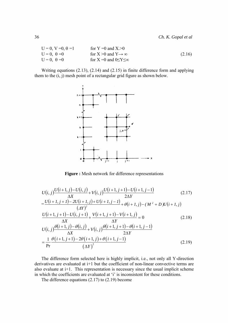
U = 0, V =0, θ =1 for Y =0 and X.>0 U = 0, θ =0 for X >0 and Y→ ∞ (2.16) U = 0, θ =0 for X =0 and 0≤Y≤∞ Writing equations (2.13), (2.14) and (2.15) in finite difference form and applying them to the (i, j) mesh point of a rectangular grid figure as shown below.

Figure : Mesh network for difference representations

( ) ( ) ( ) ( ) ( ) ( )Y

jiUjiUjiV

X

jiUjiUjiU

Δ−+−++

+Δ−+

21,11,1,,,1, (2.17)

= ( ) ( ) ( )( )

( ) ( )j,1iU)DM(j,1iY

1j,1iUj,1iU21j,1iU 2

2++−++

−+++−++ θΔ

( ) ( ) ( ) ( ) 0,11,11,1,1=

Δ+−++

+Δ

+−++Y

jiVjiV

X

jiUjiU (2.18)

( ) ( ) ( ) ( ) ( ) ( )Y

jijijiV

X

jijijiU

Δ−+−++

+Δ−+

21,11,1,,,1, θθθθ

( ) ( ) ( )( )2

1, 1 2 1, 1, 11Pr

i j i j i j

Y

θ θ θ+ + − + + + −=

Δ (2.19)

The difference form selected here is highly implicit, i.e., not only all Y-direction derivatives are evaluated at i+1 but the coefficient of non-linear convective terms are also evaluate at i+1. This representation is necessary since the usual implicit scheme in which the coefficients are evaluated at ‘i’ is inconsistent for these conditions. The difference equations (2.17) to (2.19) become


( )

( ) ( )( )

( ) ( )j,1iUX

j,iUD

m1

M

Y

21j,1iU

Y2

j,iV

Y

12

2

22+⎥

⎦

⎤⎢⎣

⎡++

+++−+⎥

⎦

⎤⎢⎣

⎡−

−ΔΔΔΔ

( )

( ) ( ) ( ) ( ) ( )X

j,iUj,iUj,1i1j,1iU

Y2

j,iV

Y

12 Δ

θΔΔ

=+−++⎥⎦

⎤⎢⎣

⎡+

−+ (2.20)

( ) ( ) ( ) ( )[ ]1,1,1,11,1 +−++ΔΔ

−+=++ jiUjiUX

YjiVjiV (2.21)

( )

( ) ( )( )

( ) ( )2 2

1, 1,1 21, 1 1,2Pr Pr

V i j U i ji j i j

Y XY Yθ θ

⎡ ⎤ ⎡ ⎤+ +−− + − + + +⎢ ⎥ ⎢ ⎥

Δ ΔΔ Δ⎢ ⎥ ⎢ ⎥⎣ ⎦ ⎣ ⎦

( )

( ) ( ) ( ) ( )2

1, 1, ,1 1, 12Pr

V i j U i j i ji j

Y XY

θθ

⎡ ⎤+ +−+ + + + =⎢ ⎥

Δ ΔΔ⎢ ⎥⎣ ⎦ (2.22)

Equations (2.20) to (2.22) together with the boundary conditions (2.16) are solved by Gauss Elimination Method which consists of solving the set of equations (2.20), (2.22) and (2.21) in that order repeatedly. Writing equations (2.20), (2.21) and (2.22) in finite difference form and applying them to the (i, j) mesh point of rectangular grid as shown in the figure. The finite difference approximation to the derivatives (2.13) to (2.15) as follows Continuity equation:

( ) ( )1, 1 1,V j k V j kV

Y Y

+ + − +∂=

∂ Δ

( ) ( ) ( ) ( )1, 1 1, , 1 ,2

U j k U j k U j k U j kU

X X

+ + − + − + −∂=

∂ Δ

Momentum equation:

( ) ( )1, ,U j k U j kU

X X

+ −∂=

∂ Δ

( ) ( )1, 1 1, 12

U j k U j kU

Y Y

+ + − + −∂=

∂ Δ

( ) ( ) ( )( )

2

22

1, 1 2 1, 1, 1U j k U j k U j kU

Y Y

+ + − + + + −∂=

∂ Δ

Energy equation:

( ) ( )1, ,j k j k

X X

θ θθ + −∂=

∂ Δ

( ) ( )1, 1 1, 12

j k j k

Y Y

θ θθ + + − + −∂=

∂ Δ


( ) ( ) ( )

( )

2

22

1, 1 2 1, 1, 1j k j k j k

Y Y

θ θ θθ + + − + + + −∂=

∂ Δ

The finite difference approximations are not perfectly symmetrical nor are they same form in all equations. This is done so as to ensure stability of the computer solution and to enable the equations to be uncoupled from each other. If small mesh spacing is used all of these forms approach the real derivative. Form the nature of the last three expressions it can be seen that (2.22) is the only expression involving the temperatures, and therefore it may be solved separately from (2.20) and (2.21). By determining an additional equation involving only unknowns which appear in (2.21), this equation may be uncoupled from (2.20) and solved separately. This additional equation or equation of constraint may be obtained by solving (2.20) to obtain the velocity at the wall V (j+1, N+1) which is zero, in terms of the center line velocity V (j+1, 0) which is also zero. The resultant equation becomes

( ) ( ) ( )1 1

( 1,0) 2 1, ,0 2 ,N N

k k

U j U j k U j U j k= =

+ + + = +∑ ∑ (2.23)

A set of simultaneous equation (2.21) together with (2.23) may be written. One equation can be formed about each mesh point in a column as shown

( ) ( )k,jU20,jU)2,1j(U2)1,1j(U2)0,1j(UN

1k∑=

+=−−−−−−−−−++++++ ,

( ) ( )0 0 0 0( 1,0) ( 1,1) 1U j U j p jβ α γ ξ φ+ + + + + − − − − −− − − − − − + + = ,

( ) ( )1 1 1 1( 1,0) ( 1,1) 1,2 1U j U j U j p jα β γ ξ φ+ + + + + + − − − − − − − + + = , --- --- --- --- --- --- --- --- --- --- --- --- --- --- --- --- --- --- --- --- --- --- --- --- --- --- --- ( )( 1, 1) ( 1, ) 1N N NU j N U j N p jα β ξ φ+ − + + + − − − − − −− − − − − − + + = , where

( )

( )2

,12k

V j k

YYα = +

ΔΔ,

⎥⎦

⎤⎢⎣

⎡++

++−=

X

)k,j(UD

m1

M

)Y(

22

2

2k ΔΔβ

( )

( )2

,12k

V j k

YYγ = −

ΔΔ,

1X

ξ −=Δ

, ( ) ( )2 ,k

P J U j k

Xφ

⎡ ⎤+= − ⎢ ⎥Δ⎣ ⎦

This set of equations can be solved by Gauss-Jordan Method. Application of the


newly found axial velocities (U’s) together with those in the column behind into equation (2.20) determines the new transverse velocities (V’s). Equation (2.20) can be written as using finite-difference equations as shown

( 1, 1) ( 1, ) [ ( 1, 1)2

YV j k V j k U j k

X

Δ+ + = + − + +

Δ

( 1, ) ( , 1) ( , )]U j k U j k U j k θ− + − + − + The set of velocities are now placed into a set of finite-difference equations written about each mesh point in a column for the equation (2.22) as shown ( )00 0 0( 1,0) ( 1,1)j jβ θ α γ θ φ+ + + + + −−−−−−−−−−−−−−− = ,

( )1 1 1 1( 1,0) ( 1,1) 1, 2j j jα θ β θ γ θ φ+ + + + + + −− − − − − − − − − −− = , --- --- --- --- --- --- --- --- --- --- --- --- --- --- --- --- --- --- --- --- --- --- --- --- --- --- --- ( 1, 1) ( 1, )N N N Nj N j Nα θ β θ φ γ+ − + + = − , where

( )

( )2

,12Pr

kV j k

YYα = +

ΔΔ,

( )( )

2

,2Pr

k

U j k

XYβ

⎡ ⎤= − +⎢ ⎥

ΔΔ⎢ ⎥⎣ ⎦

( )

( )2

,12Pr

k

V j k

YYγ = −

ΔΔ, ( ) ( ), ,

k

U j k j k

X

θφ = −

Δ

The same techniques may be used to solve this set of equations as were used to solve the momentum equation. Finally, we find the skin friction analytically and discussed computationally with reference to different variations in the governing parameters. Results and Discussion The flow governed by the non-dimensional parameters M the Hartmann number, D the Darcy parameter and Pr the prandtl number. The figures (1-6) and (7-12) represent the velocity and the temperature profiles for X=0 and X=1 levels respectively with reference to different variations in the governing parameters being other parameters fixed. We are fixing non-dimensional stream wise velocity U as well as V non-dimensional transverse velocity. The Fig.(1-3) and fig.(8-10) represent the velocity profiles at levels X=0 and X=1; The Fig.(4-7) and fig.(11-14) represent the temperature profiles at levels X=0 and X=1, while the tables (I-II) represent the skin friction coefficient at upper and lower walls. We notice that the velocity component reduces with increasing the intensity of the magnetic field M and enhances with increasing the Darcy parameter D. Lower the permeability of the porous medium lesser the fluid speed in the entire region (Fig. 1-2). The velocity component enhances


with increasing the hall parameter m (Fig. 3). The temperature experiences retardation with increasing the intensity of the magnetic field M (Hartmann number) while it enhances with increasing the Darcy parameter D, Prandtl number Pr and hall parameter m (Fig. 4-7). Likewise the similar behaviour of the flow at X=1 level with reference to different variations in the governing parameters (Fig. 8-14). From the above we observe that the velocity of the fluid motion is decreases with increase in the magnetic parameter M. The behaviors of velocity happen with the intention of the induced magnetic field effects the fluid motion containing the porous medium. Likewise the porous medium effects the velocity of the clean fluid region since the magnitude of the velocities in the clean fluid region relatively high comparable to filling with porous materials throughout the fluid region. The skin friction at the lower wall enhances with increasing the intensity of the magnetic field M (Hartmann number) and hall parameter m, while it reduces with increasing the Darcy parameter D. Similarly the skin friction at the upper wall enhances with increasing both the intensity of the magnetic field M and the Darcy parameter D but it reduces with increasing the hall parameter m. The Velocity and Temperature profiles at level X=0:

Figure 1: The velocity profile for different M with D=1, Pr =0.71, m=1

Figure 2: The velocity profile for different D with M=2, Pr =0.71, m=1


Figure 3: The velocity profile for different m with D=1, Pr =0.71, m=1

Figure 4: The temperature profile for different M with D=1, Pr =0.71, m=1

Figure 5: The temperature profile for different D with M=2, Pr =0.71, m=1


Figure 6: The temperature profile for different Pr with M=2, D =1, m=1

Figure 7: The temperature profile for different m with M=2, D =1, Pr=0.71 The Velocity and Temperature profiles at level X=1:

Figure 8: The velocity profile for different M with D=1, Pr =0.71, m=1


Figure 9: The velocity profile for different D with M=2, Pr =0.71, m=1

Figure 10: The velocity profile for different m with D=1, Pr =0.71, m=1

Figure 11: The temperature profile for different M with D=1, Pr =0.71, m=1


Figure 12: The temperature profile for different D with M=2, Pr =0.71, m=1

Figure 13: The temperature profile for different Pr with M=2, D =1, m=1

Figure 14: The temperature profile for different m with M=2, D =1, Pr=0.71


Table I: Skin friction coefficient (τ ) at X=0 level

I II III IV V M=2 0.161228 0.142625 0.125552 0.185542 0.255652 M=5 0.244668 0.215515 0.185595 0.366526 0.558585 M=8 0.395652 0.261145 0.232551 0.411521 0.655685 M=10 0.532556 0.396655 0.265528 0.744854 0.900145

I II III IV V

D 1 2 3 1 1 m 1 1 1 2 3 Pr 0.71 0.71 0.71 0.71 0.71

Table II: Skin friction coefficient (τ ) at X=1 level

I II III IV V M=2 0.275345 0.399642 0.465552 0.225652 0.185454 M=5 0.344549 0.445852 0.585855 0.266585 0.225651 M=8 0.655281 0.801142 0.964663 0.399856 0.300258 M=10 0.797655 0.965555 1.302265 0.512215 0.385545

I II III IV V

D 1 2 3 1 1 m 1 1 1 2 3 Pr 0.71 0.71 0.71 0.71 0.71

References

[1] Al-Nimr,M.A ., and M.A.Hader., Chemical Engineering Science, vol. 54 (1999), pp. 1883-1869.

[2] Attia ,H.A., Turkish J Phys; Vol. 29,(2005), pp. 379-388. [3] Barletta,A., Int. J. Heat Mass Transfer, vol. 41 (1998), pp. 3501-3513. [4] Bejan, A., Dincer, I., Lorente, S., Miguel, A. F. and Reis, A. H., Springer, New

York (2004). [5] Bejan, A., Convective Heat Transfer, 2nd ed., Wiley, New York (1995). [6] Bhadauria,B.S., ASME J. Heat Transfer, vol. 130 (052601) (2008), p. 9. [7] BhadauriaB,S., ASME J. Heat Transfer, vol.129 (2007), pp. 835-843. [8] Chamkha,A.J., and M.M.A. Quadri., Numer. Heat Transfer, Part A 40 (2001),

pp. 387-401. [9] ChamkhaA.J.A., and R.A. Khaled., Numer. Heat Transfer, vol. Part A 36

(1999), pp. 327-344. [10] El-Amin,M.F., J. Magn. Magn. Mater., vol.261 (2003), pp. 228-237.


[11] El-Hakiem,M.A., J.Magn. Magn. Mater. vol. 220 (2000), pp. 271-276. [12] Ettefagh, J., Vafai, K., and Kim, S.J., J. Heat transfer, vol. 113 (1991), pp. 747-

753. [13] Georgantopoulos, G. A., Koullias, J., Goudas, C. L., and Courogenis, C.,

Astrophys. Space Sci., vol. 74 (1981), p. 357. [14] Ghaly,A.Y., Chaos Solitons Fract. vol. 13 (2002), pp. 1843-1850. [15] Gounder Ganesan,P., and P. Hari Rani., Int. J. Therm. Sci. 39 (2000), 265-272. [16] Guillaume Polidori and Catalin Popa, and Ton Hoang Mai., Mechanics

Research Communications, vol. 30 (2003), pp. 615-621. [17] Harris,S.D., L. Elliot., D.B. Ingham., and I. Pop., Int. J. Heat Mass Tran., vol.

41(1998), pp. 357-72. [18] Ingham, D. B., and Pop, I., Transport Phenomena in Porous MediaII Pergamon,

Oxford (2002). [19] Ingham, D. B., and Pop, I., Transport Phenomena in Porous Media III.

Elsevier,Oxford (2005). [20] Kamel, M.H., Energy Convers Manage; vol, 42(4) (2006), pp. 393-405. [21] Kassem,M., Int. Commun. Heat Mass transfer, vol. 20 (2006), pp. 333-345. [22] Kou, H.S., and Lu. K.T., Int. Commun. Heat Mass transfer, vol. 20 (1993), pp.

333-345. [23] Krishna, D.V. ,Prasada Rao .D.R.V., and Ramachandra Murthy.A.S.,

Inzhenerno-Fizicheskii Zhurnal; vol. 75(2) (2002), pp. 12–21. [24] Kumari.M, H.S., Takhar., and G. Nath., Heat Mass Transfer, vol. 37 (2001), pp.

139-146. [25] Malashetty, M.S., and J.C. Umavathi., International Journal of Non-Linear

Mechanics, vol. 40 (1999), pp. 91-101. [26] Mansour,M.A., and N.A. El-Shaer., J. Magn. Mater., vol. 250 (2002), pp. 57-

64. [27] Nield, D. A., and Bejan, A., Convection in Porous Media, 2nd ed., Springer,

New York (1999). [28] Nield, D. A., and Bejan, A., Convection in Porous Media, third ed., Springer,

New York (2006). [29] Pantokratoras,A., Appl. Math. Model., vol. 29 (2005), pp. 125-135. [30] Polidori, G., C. Popa., and T. Hoang-Mai., Mech. Res. Commun., vol.

30(2003), pp. 515-621. [31] Pop, I. and Ingham, D. B., Convective Heat Transfer: Mathematical and

Computational Modelling of Viscous Fluids and Porous Media, Pergamon, Oxford (2001).

[32] Postelnicu,A., Int. J. Heat Mass Transfer, vol. 47 (2004), pp. 1467-1472. [33] Rakoto Ramambason,D.S., and P. Vasseur., Acta Mech., vol. 191 (2007), pp.

21-35. [34] Rastogi, S.K., and D. Poulikakos., Int. J. Heat & Mass Transfer, vol. 38 (1995),

pp. 935-946. [35] Seddeek,M.A., J. Appl. Mech. Tech. Phys., vol. 43 (2002), pp. 13-17. [36] Soundalgekar ,VM., Vighnesam, NV., and Takhar, H.S., IEEE Trans Plasma

Sci; vol. 7 (1979), pp. 178-82.


[37] Soundalgekar, V. M., J. Appl. Math. Mech., vol. 55 (1975), p. 257. [38] Soundalgekar, V. M., J. Heat Transfer, Trans. ASME, vol. 99 (1977), p. 499. [39] Soundalgekar, V. M., Free convection effects on the oscillatory flow past an

infinite, vertical porous plate with constant suction I. Proc. 1%. Soc. (London) vol. 888 (1973), p. 25.

[40] Soundalgekar, V. M., Free convection effects on the oscillatory flow past an infinite, vertical porous plate with constant suction II. Proc. 1%. Soc. (London) 888 (1973), p. 37.

[41] Soundalgekar,V.M., B.S. Jaiswal., A.G. Uplekar., and H.S. Takhar., Appl. Mech. Eng., vol. 4 (1999), pp. 1-25.

[42] Sparrow, E. M., and Gregg, J .L. Trans ASME, vol. 78, (1956), p. 435. [43] Vafai, K., Handbook of Porous Media, Marcel Dekker, New York (2000). [44] Vafai, K., Handbook of Porous Media, 2nd ed., Taylor & Francis, New York

(2005).

Finite Difference Analysis on Hall Current Effects on … Dr. B.D.C.N. Prasad3 1Dept. of...

Documents

Transcript of Finite Difference Analysis on Hall Current Effects on … Dr. B.D.C.N. Prasad3 1Dept. of...