Limnul Oceanogr, 49(4, part 2). 2004, 1446-1456C 2004, by the American Society of Limnology and Oceanography, Inc.

Fingerprints of biocomplexity: Taxon-specific growth of phytoplankton in relation toenvironmental factors

John T. LehmanNatural Science Building, University of Michigan, Ann Arbor, Michigan 48109-1048

Sally E. B. Abella, Arni H. Litt, and W. Thomas Edmondson'Department of Zoology, University of Washington, Seattle, Washington 98195

Abstract

Phytoplankton and environmental conditions in Lake Washington, Seattle, Washington, are discussed from theperspective of dynamic relationships between taxon-specific growth rates and environmental variables. More thanfour decades of measurements permit inspection of conditions associated with net increase and decrease for 40phytoplankton species or species groups. Reproducible patterns exist for growth responses to over 25 environmentalfactors including nutrient chemistry, physical variables, and herbivorous zooplankton species. There appear to beno more than six main modalities of response to environmental factors, and responses to chemical and physicalvariables show coherence across taxa. Diatoms show a near uniform positive growth response to abundant inorganicnutrients, cold and transparent water, deep mixing, and intolerance for virtually all zooplankton grazers. Manychlorophytes and cyanobacteria show equally uniform growth responses to chemical and physical variables, althoughtheir preferences are virtually opposite from the diatoms. They benefit from the presence of copepods but showhighly specific growth rate responses to different cladocerans and rotifers. Growth rate variations among the diatomssort out along gradients of resource and physical factors, but there is coherence to the rise and fall of multiplespecies. Among the other algal divisions, despite a common set of physical and chemical conditions that promotegrowth rates, the species do not increase and decrease together. Instead, the prevailing grazer community appearsto shape the phytoplankton community by admitting only certain species from the large pool of contenders.

The idea of using distributions and dynamics of organismsto deduce evolutionary adaptive strategies that allow speciesto propagate and prosper has proved illuminating for bothterrestrial plant and phytoplankton ecologists (Margalef1978; Grime 1979; Reynolds 1988). Strategies have beendefined as traits that permit a taxon or group of taxa to be-come better suited to particular sets of environmental con-ditions. Both Grime and Reynolds have argued that variousstrategies have tended to sort out along three major axes orlines of adaptive specialization. They identify "stress," "dis-turbance," and "competition" as the key themes that shapeplant communities by natural selection.

When we inspect natural communities, however, there isa challenge in attempting to reconcile these concepts (e.g.,stress) with specific environmental measurements. Stress,disturbance, and competition are abstractions of natural phe-nomena, and hence they have no objective existence that ismandatory for unambiguous, reproducible measurement.This is not meant to decry the value of metaphor in systemsas complex as biological communities, but it does suggest

I Deceased.

AcknowledgmentsW. Thomas Edmondson passed away 10 January 2000 after we

had started the work on this paper. The long record of data on LakeWashington comes from the work of many colleagues: technicians,students, postdoctoral associates, and volunteers. The most directlyinvolved included Katie P. Frevert, the late David E. Allison, andthe late Mardi I. Varela. The work was supported by a series ofgrants from the U.S. National Science Foundation and by the An-drew W. Mellon Foundation.

the need for approaches to adaptive strategies that link tight-ly with environmental data. Open water communities ofplanktonic algae have commanded scrutiny ever since G. E.Hutchinson articulated the "paradox of the plankton" tohighlight the existence of profound biodiversity within a su-perficially homogeneous medium. Reconciliation of the par-adox requires demonstration of the true complexity that ex-ists within that world, and strict demonstration calls for morethan analogy and metaphor.

Few data sets permit detailed inspection of the complexinterrelationships among phytoplankton dynamics, waterchemistry, lake physics, and herbivore communities over de-cadal time scales, but Lake Washington at Seattle offers suchopportunity. Long-term changes in the phytoplankton com-munity of that lake during the second half of the 20th cen-tury have recently been described (Edmondson et al. 2003),along with an introduction to associated physical and chem-ical variables. The report by Edmondson et al. focused oninterannual variations and on the major phytoplankton tran-sitions that accompanied alterations in nutrient income andherbivore community.

We here turn our attention from describing the long-termcommunity transformations to inquiries about the mechanis-tic basis for species success, decline, and community tran-sitions. The time period for this study spans 5 decades andencompasses dramatic episodes of cultural eutrophicationand recovery, as well as progressive land development, wa-tershed management, and manipulation of fish communities.Previous work has divided the long interval into three majoreras: eutrophication (1941-1968), recovery (1969-1975),and Daphnia era (1976-present). In this study we will re-

1446

Phytoplankton growth in Lake Washington

focus from the temporal mesoscale (seasons to years) to ex-amine the growth patterns and associated environmental var-iables at week to week scale throughout the entire period ofrecord.

Approximately 40 phytoplankton taxa have been charac-terized as key elements in the changing lake community ofLake Washington (Edmondson et al. 2003). The aim of thispaper is to examine the environmental conditions that existduring times of net positive growth (increase) as well as netnegative growth (decrease) for the key taxa individually andfor various aggregated groups. This approach permits rec-ognition of consistent patterns as well as formulation of hy-potheses about differential roles of physical, nutrient chem-ical, and grazer control factors in the rise and fall ofindividual or allied taxa.

Methods

Description and reconciliation of the time series data-The first step in this analysis was to construct a commontime basis for intercomparison of diverse data types. Thespecific methods used to collect and measure each variableare described by Edmondson et al. (2003). Observations ofweather conditions, lake physics, water chemistry, phyto-plankton biovolume, crustaceans, and rotifers were not al-ways simultaneous.

Lake chemistry data for the surface mixed layer (TP [totalP after perchlorate oxidation], DP [filterable P after perchlo-rate oxidation], SRP [soluble reactive P], raw PO,-P [unfil-tered molybdate reactive P04 -P], SN [total Kjeldahl N: NH,-N + organic N], NO,-N, NO,-N, NH,-N, SRSi [solublereactive Si], ANC [acid neutralizing capacity, or titration al-kalinity], and pH) were treated as contemporaneous if theywere measured within 24 h of each other. Replicate valuesobtained on a single date were averaged.

Observations of Secchi transparency depth, mean temper-ature of the surface mixed layer (T.,J, and depth of themixed layer (Z,i.) were treated as contemporaneous if thedates were within 24 h of each other. Additional estimatesfor Secchi depth needed to correspond with T,,,,x and Zn,hwere obtained by linear interpolation. These supplementalderived values were combined with the primary data andinitially tracked as a separate (derived) variable: SDinte,. Dai-ly records for insolation and wind speed were averaged forthe dates between Tm.x and Zmix sample dates. The resultingvariables Mean I,, and Mean Wind thus represented meanvalues over a sampling interval. An index variable for meanlight intensity in the mixed layer was derived as

1iea_ = Mean io/(Zmix/SDine,,p) (I)

Zooplankton abundances were expressed as animals per cu-bic meter and were arrayed on a common time grid usingthe same criteria for contemporaneous values as were ap-plied to the chemistry and physical variables and averaging.Biovolume estimates for phytoplankton taxa were expressedas mm3 L-'.

The sampling interval varied seasonally and to some de-gree across the years. Sampling was typically weekly fromMarch to October and biweekly or occasionally triweekly atother times. However, in some years the weekly regime was

maintained for the full year. From 1962 to 1997, the meansampling interval was 11.1 d (SD = 5.2 d).

Growth phase characterization-A protocol implementedin Microsoft ExcelTM was developed to identify periods ofsustained increase or decrease in algal taxon groups:

1. Dates were flagged positive (POSflag) if they were partof a series of at least four consecutive monotonically in-creasing values of biovolume for the specified taxon.

2. Dates were flagged negative (NEGflag) if they werepart of a series of at least four consecutive monotonicallydecreasing values of biovolume for the specified taxon.

3. Neither endpoint of the monotonic biovolume serieswas counted in either the POSflag or NEGflag series.

4. POSflag and NEGflag date masks developed from tax-on-specific phytoplankton biomass (binary flags: 0 or I)were used to identify environmental variables on the asso-ciated dates.

5. POSflag and NEGflag date masks were used to extractthe full set of environmental variables associated with positiveor negative growth intervals, as defined in steps I and 2.

6. Summary statistics and comparisons were performedon the extracted data in order to compare the attributes ofenvironmental variables during times of positive and nega-tive net growth rates that were taxon specific.

The adopted protocol represented a conservative way toidentify periods of sustained increase and to segregate themfrom periods of sustained decrease. Our reasoning was thatisolated jumps or drops in biovolume from one samplingdate to the next could arise from many causes includingartifacts, and it could not be certain whether the environ-mental conditions at each such date were associated withpositive, negative, or indeterminate population growth. If anet growth trajectory was maintained across at least foursample dates, however, we considered it justifiable to regardthe environmental conditions during the core dates of theinterval (e.g., dates two and three for a four-date monotonicseries) as being indicative of conditions permissive of netincrease or net decrease.

Prior to statistical comparisons, the environmental vari-ables including zooplankton abundances were subjected toinspection and statistical test for symmetry and normality.Transformations were applied to the variables to permit ap-plication of parametric statistical tests whenever appropriate.In order to permit logarithmic transformation in cases whenanalytical results yielded chemical concentrations that wereindistinguishable from blank (zero concentration), the"zero" values were adjusted to the approximate minimumvalues of analytical detection as reported in the data set. Theadjustment values and numbers of cases affected were asfollows:

DP:

SRP:

+ 1.0 gg L (6 cases out of 758)

+0.2 ,ag L-' (55 cases out of 852)

raw P04 -P: +0.2 ag L-' (89 cases out of 1,038)

N0 3-N:

NO2 -N:

NH3-N:

+2 pg L-' (28 cases out of 957)

+0.1 Ag L (126 cases out of 392)

+0.2 pkg L-' (72 cases out of 370)

1447

Lehman et al.

Table 1. Descriptive statistics for the environmental variables used to test for differences between positive net growth and negative netgrowth by different phytoplankton taxa. Variable names that begin with "LN" indicate that the native data were transformed by naturallogarithm. Unless indicated otherwise, water chemistry variable units are Ag L-' before transformation. Insolation (Mean 1o and 'men) arein g-cal cm-2 d-'; wind speed is m s-'. Chemistry data range from 14 Jan 1933 to 24 Mar 1999. Physical data range from 7 Jan 1950 to24 Mar 1999.

Variable name Mean Median SD n Min Max

LN(TP) 2.85 2.82 0.64 874 0.69 4.63LN(DP) 2.13 1.97 0.80 758 0.00 4.36LN(raw P04 -P) 1.17 0.99 1.54 1,038 -1.61 4.13LN(SRP) 1.00 0.77 1.48 852 - 1.61 4.08SRSi (mg L-') 1.62 1.58 0.805 475 0.01 3.46LN(IN) 5.68 5.62 0.42 438 3.74 6.98LN(NO,-N) 4.38 4.80 1.39 957 0.69 6.30LN(NO-N) -0.82 -0.92 1.37 392 -2.30 3.43LN(NH 3-N) 1.58 2.17 1.80 370 -1.61 5.16ANC (mEq) 0.68 0.68 0.082 957 0.28 0.82PH 7.96 7.80 0.625 982 6.3 9.95Secchi (m) 5.0 5 2.2 1,993 0.7 12.9SDi.,,, (m) 4.9 4.8 2.2 2,146 0.7 12.9Zm,x (m) 26.5 14 23.6 1,655 1 65Tmix (m) 13.4 13.3 5.1 1,655 4.2 23.8Mean 10 309.6 309.4 172.8 2,059 29.6 755.6Mean wind 8.1 8.1 1.7 2,001 1.4 14.42Imean 140.6 73.7 192.9 1,574 1.6 2,410.4

Table 2. Descriptive statistics for the natural logarithm transfor-mations of nonzero zooplankton abundances (animals m-3) by taxonand life stage. Abundance data range from 11 Feb 1950 to 30 Nov1998. Dg = Daphnia galeata; Dt = Daphnia thorata.

Medi-Ln-transformed Mean an SD n Min Max

Diaptomus C6 7.58 7.67 1.10 1,307 0 10.35Diaptomus Cl-C6 9.14 9.11 1.16 1,316 3.33 12.25Epischura C6 4.12 4.29 1.72 1,200 0 8.37Epischura Cl-C6 5.38 5.53 1.72 1,269 0 9.08cyclopoids CI-C6 8.89 8.91 0.94 1,315 3.91 11.66Diaphanosoma 5.34 5.32 2.30 842 0.69 10.24Bosmina 5.56 5.58 1.95 1,088 0.69 10.99Daphnia adults 5.81 6.44 2.35 797 0 9.58Daphnia total 6.75 7.54 2.64 890 0 10.89D. ptulicaria adults 5.45 6.00 2.29 719 0 9.55D. pulicaria total 6.46 6.97 2.5 1 772 0.47 10.84Dg + Dt adults 5.06 5.28 1.99 598 0.41 9.27Dg + Dt total 5.86 6.18 2.36 661 0.47 10.29Conochilus unicornis 7.11 6.91 2.32 467 2.30 12.73Conochilus hippocrepis 7.94 7.78 2.17 310 1.61 13.71Keratelta quadrata 5.53 5.43 1.48 357 2.20 10.76Keratella cochlearis 7.57 7.29 2.31 995 2.48 14.69Kellicottia longispina 7.84 7.88 1.79 1,113 2.56 13.53Notholca 5.23 5.23 1.18 76 3.00 7.85Polyarthra 7.70 7.68 2.00 949 2.48 13.28Ascomorpha 5.44 5.24 1.42 135 2.30 9.65Trichocerca 5.94 5.76 1.91 280 2.20 13.21Ploesoma 5.31 5.36 1.19 36 3.30 8.67Filinia 5.62 5.62 1.53 107 2.77 9.99Synchaeta pectinata 6.25 6.09 1.77 240 2.08 10.86Other Synchaeta 6.18 6.13 1.74 358 2.30 11.34

In order to ascertain the number of orthogonal axes (inde-pendent variables) represented in fact by the data sets, eachdata set (chemistry, physics, zooplankton) was subjected toprincipal components analysis (Systat 5.01) weighting thevariables according to their correlations.

Results

Transformation of variables-Most of the environmentalvariables exhibited skew characteristic of lognormal distri-butions (e.g., serious departure of mean/median ratios from1.0) that could be largely corrected by logarithmic transfor-mation. Table I lists descriptive statistics for the global setof chemical and physical variables that was ultimately usedin this study. Transformation was applied to all water chem-istry variables except pH, ANC, and SRSi. Physical vari-ables appeared suitable for use without transformation, withtwo exceptions. Both Zmix and Imean (derived from ZmJx) havebimodal distributions, and hence neither one can be trans-formed to approximate a symmetrical Gaussian shape. Sta-tistics applied to these variables must therefore be interpretedwith due caution.

Zooplankton frequency distributions were all strongly log-normal. Transformation by natural logarithm produced sym-metrical unimodal distributions (Table 2).

Principal components analyses (PCA) revealed that fiveindependent axes are required to represent 95% of the var-iance within the chemistry data set. Five independent axeswere needed to account for 95% of the variance in the phys-ical variables, as well. Orthogonal transformation of the var-iable axes was not conducted, however. Variables were con-temporaneous (all variable measurements availablesimultaneously) on only 1,353 of 2,136 dates for physicalvariables and on only 271 of 1,249 dates for chemical var-

1448

Phytoplankton growth in Lake Washington1

Table 3. Descriptive statistics for the natural logarithm transformations of nonzero algal biovolume (mm3 L-') by taxon. Data timeperiod ranges from II Feb 1950 to 22 Dec 1997. See Edmondson et al. (2003) table 3 for more detail about the taxa included in aggregatedcategories.

Ln-transformed ID Mean Median SD n Min Max

Oocystis gigasOther Oocystis spp.Staurastrum paradoxumGelatinous greensAcicular greensBotryococcus spp.Other greensAsterionella formosaCyclotella pseudostelligeraC bodanica + C. coinraC. ocellataDiatoma elongatumFragilaria crotonensisAulacoseira subarcticaAtulacoseira italica v. tenuissimaMelosira variansRhizosolenia eriensisSteph. neoastraea + S. minutulaSteph. hantzschii + S. alpinusSteph. niagaraeLarge Synedra spp.Synedra teneraTabellaria fenestrataOther diatomsMallomonas spp.Chroomonas ininutaCryptomonasAnabaenaAphanizomenonChroococcus limneticusCoelosphaeriumMicrocvstisLyngbya limneticaOscillatoriaPseudanaboenaSchizothrixOther colonial coccoid bluegreensOther bluegreensCerarium hirundinellaOther dinoflagellatesAll othersTotal (1-41)

GIG2G3G4G5G6G7D8D9DIODIID12D13D14D15D16D17D18119D20D21D22D23D24M25C26C27B28B29B30B31B32B33B34B35B36BB37B38F39F40041T42

-3.35-6.22-4.89-5.85-6.78-3.78-5.92-4.44-7.52-4.74-5.99-3.19-3.92-3.11-4.98-4.50-5.65-4.35-5.84-1.33-5.45-5.91-2.89-6.18-5.88-4.72-3.42-4.96-5.11-5.48-5.59-5.97-5.04-1.33-4.57-4.04-6.70-6.94-2.42-5.61-3.20

0.40

-3.38-6.15-4.84-5.72-6.65-3.69-5.79-4.47-7.72-4.76-6.03-3.59-3.95-3.09-4.99-4.37-5.83-4.44-6.20-1.44-5.57-6.02-2.92-6.22-5.98-4.52-3.39-5.20-5.07-5.51-5.60-6.11-4.93-1.09-4.83-4.09-6.64-7.06-2.24-5.59-3.19

0.33

1.521.321.131.541.391.731.391.741.691.401.462.602.051.891.561.301.671.811.731.56'.771.671.981.82'.341.301.382.181.911.38'.731.902.302.071.482.241.802.411.161.280.861.13

339465195722921

57762729411146289

61890868563131315526297412782243270968375

1,1121,109

694613237391183511466

46273482289

55311

1,2481,252

-6.90-11.11-7.03

-10.41-11.87-7.75

-10.48-8.77

-11.18-8.52

-10.01-9.21-9.57-9.50-8.87-7.80-9.61-8.91

-10.01-6.36

-10.52-9.16-7.12

-11.11-10.18

-9.17-8.06

-10.68-9.76-8.92

-12.72-9.40

-13.12-9.63-7.78-9.88

-11.51- 12.43-5.93-9.53-7.82-2.37

0.24-2.41-1.50-2.11-1.71-0.91-2.85

1.73-1.67-0.69-1.51

1.171.450.80

-0.59-0.74

0.830.33

-0.662.64

-0.51-1.55

1.740.21

-1.80-0.86

0.322.120.18

-0.820.530.220.942.54

-1.101.11

-1.28-0.82-0.53-2.13-0.41

3.56

iables. The reduction in power and resolution that wouldresult from a transformation of the coordinates was deemednot worthwhile. It was easy to understand that there werehigh correlations among several of the variables and that theresults could be interpreted by considering them as a suite.For example, 57% of the overall variance in the water chem-istry data could be assigned to a single axis that was dom-inantly constructed of SRP, DP, raw P04 -P, NO3 -N, and SRSi(positive correlations) plus ANC (negative correlation). Thesecond major component of variance (20% of total) wasdominated by EN and NH3 (positive correlations). The thirdelement (12% of total variance) was dominated by TP (neg-ative loading) and NO2 (positive). These results elucidate thesomewhat obvious large-scale features of a data set that con-

tains data from eutrophic years as well as from unenrichedconditions.

Zooplankton abundances by taxon also exhibit correla-tions. Principal components analysis applied to the zoo-plankton data revealed that 12 orthogonal axes are requiredto account for 95% of the variance in the data. There wassome obvious redundancy in the data set stemming fromnested variable categories. For example, adult Diaptomusand adult Epischura correlate necessarily with total cope-podids of each taxon (r = 0.637 and 0.799, respectively).Abundance of adult Daphnia correlates tightly with totalabundance of Daphnia (r = 0.965), adult Daphnia pulicaria(r = 0.928), total D. pulicaria (r = 0.881), and total D.galeata plus D. thorata (r = 0.817).

1449

Lehman et al.

G G GVariable 1 2 3TPDP

Po,rawSRP M

SRSi

NO

N02

Nli.

pH LANC m

12 3SecchuSD rterp

TiaramvCMeanWirad

Diaptoms C06

Epschura C6 L .Eptsrhura C -C6cyclopoid 0 Cl-C6DiaphanosomaBosminaDaphmu adAlts ,Daphma TotalDpulicofla adults LiDpulicanza TotalDg+Dt adultsDg+Dt TotalC unkornisConochilushIppocrepis mKemaelfa quadralaKeratelia coc NearlsKelicotia longispanaAobokaPalyritraAsconwerpha .I7Thhocerca L2Ploetoma1inia

Syclhaeapectbed-aOtherSynchaeta

G G G D D D4 5 7 8 9 10

D D D D D D DD D DD DO D M C C B BI 1 12 13 14 15 16 17 18 19 20 21 22 23 24 25 26 27 28 29wts s g _

1E tA' +0:

B B B B B B B B B F F O30 31 32 33 34 35 36 37 38 39 40 41

AA g

e *F- ._

Fig. 1. Net growth relationships between individual algal taxa and environmental variables. Gray denotes that the net positive growthis associated with statistically higher values of the environmental variable (positive relationship between variable and growth rate). Blackdenotes that net negative growth is associated with statistically higher values of the variable (negative relationship). White indicates thatno consistent, statistically significant relationship could be established between growth rate and the variable.

The results from PCA were used as a guide for the num-bers of independent variables that could realistically be in-spected for effects on algal growth rates. Table 3 lists thealgal taxa that were investigated. The longevity of the LakeWashington data set has the disadvantage that taxonomicrevisions have affected many of the species studied overtime, for example some of the bluegreen algae (Anagnostidisand Komarek 1988). Nonetheless, for consistency of report-ing and for comparison with our previous publications, wehave retained the older names in this paper. For each taxon,environmental variables (Tables I and 2) extracted duringtimes of net positive growth and net negative growth werecompared by two-tail t-test to ascertain whether the two sub-sets differed in mean value. If the mean values differed ata = 0.05, the variable was flagged to differentiate whetherthe value of the environmental variable was greater duringtimes of net positive growth or net negative growth.

Figure 1 illustrates the resulting environmental "finger-

prints" from the statistical tests by taxon. Because of thehigh correlations and consistency of responses among allmeasured forms of phosphorus, a composite variable P varswas defined to represent the collective responses to TP, DP,SRP, and raw P04 -P Because of consistency of responseacross taxa, NH3 and NO2 were combined with IN. Thisreduced the number of water chemistry variables to six,which is close to the five orthogonal axes identified by PCA.Further consolidation would have been possible by combin-ing silica or nitrate with phosphorus, but we decided to retainthe identification of these different elements.

The physical variable set was reduced to five by discard-ing Secchi in favor of the supplemented data series SDintel,

and we aggregated T .. and Mean 14 as "heat vars."The zooplankton variable set was reduced to 13 by first

aggregating the two Diaptomus categories as "Diaptomus,"and the two Epischura categories as "Epischura." Then, fivehighly correlated Daphnia categories were aggregated as

1450

40 41

40 41

II

-

~~~~ p 1 E 1

IU

ED

Phytoplankton growth in Lake Washington

Table 4. Environmental variables, including aggregate variables,and the number of taxon-specific cases for each when positive netgrowth rates occurred at significantly larger values of the variablethan did negative net growth rates (i.e., there is a positive correla-tion between the environmental variable and net growth). "Grns"= Greens (GI-G7); "Dtms" = Diatoms (D8-D24); BGs = Blue-greens (B28-B38); "Flgs" = Flagellates (M25, C26, C27, F39,F40); "All" = All taxa (1-41); "BV" = total biovolume. Fre-quencies are taken from the complete data set (Fig. 1).

Variable All BV Grns Dtms BGs Figs

P vars 63 3 4 49 4 4SRSi 10 I 0 9 0 1NO3 12 1 1 10 0 1IN 7 0 2 l 4 0pH 9 0 2 0 6 1ANC 3 0 1 l 0 0SD1 ,11~,P 12 1 1 9 1 1

Z.il 15 1 1 13 0 1Heat vars 23 0 6 1 14 2Mean wind 7 0 1 5 1 0

14 0 3 l 7 3Diaptomnus 21 0 6 5 8 1Epischura 17 0 6 0 10 1Cyclopoids 5 0 1 0 3 1Diaphanosoma 2 0 0 0 2 0Bosmina 3 0 0 0 3 0Daphnia 14 0 3 0 l l 0DgDt tot 2 0 1 0 1 0C. unicornis 5 0 2 0 2 1C. hippocrepis 4 0 1 2 0 1Rotifers A 16 0 1 2 13 0Polyarthra 7 0 3 1 3 0Ascomorpha 4 0 1 2 1 0Rotifers B 16 0 3 2 9 2

"Daphnia"; Keratella, Kellicottia, and Notholca were ag-gregated as "Rotifers A"; and Trichocerca, Ploesoma, Fili-nia, and all Synchaeta were aggregated as "Rotifers B."

In every case among the aggregated variables there wereno inconsistencies within the member categories in terms ofstatistically significant response patterns. Taxon-specific fre-quencies of positive or negative growth response to eachenvironmental variable are listed in Tables 4 and 5. We usedthe full count of statistically significant responses identifiedin the complete data set (i.e., Fig. 1) but assigned the countsto aggregated variables subsequently identified. Summarytaxon-specific fingerprints of the condensed environmentalvariable suite are illustrated in Fig. 2.

Frequency distributions reported in Tables 4 and 5 weretested for homogeneity across taxa by chi-squared analysis.Simultaneous analysis of four aggregated taxon categories(greens, diatoms, bluegreens, and flagellates) revealed strik-ing inhomogeneities (p = 6.1 X 10- ' for positive growthrate correlations and p = 1.1 X 10-16 for negative growthrate correlations). Pairwise contrasts among the four taxongroups likewise revealed strong differences in response toenvironmental variables (Table 6). Extraordinarily strong sta-tistical differences exist between diatoms and every othertaxon as well as between bluegreens and flagellates duringpositive growth phases. These statistical differences refer to

Table 5. As Table 4, but listing the number of taxon-specificcases for each environmental variable when negative net growthrates occurred at significantly larger values of the variable than didpositive net growth rates (i.e., there is a negative correlation be-tween the environmental variable and net growth).

Variable All BV Gms Dtms BGs Flgs

P vars 17 0 4 0 l l 2SRSi 4 0 2 0 2 0NO, 4 0 0 0 4 0IN 6 l 0 6 0 0pH ll I 0 11 0 0ANC 3 0 1 0 1 1SDii,t.rp 5 0 1 l 3 0Zm,x 10 0 3 1 6 0Heat vars 29 1 1 25 1 2Mean wind 5 0 0 0 3 2II-ea 8 0 0 8 0 0Diaptomus II 0 0 10 0 1Epischura 19 2 0 19 0 0Cyclopoids 8 1 0 7 0 1Diaphanosoma 16 1 2 12 1 0Bosmina 12 1 1 7 2 1Daphnia 63 5 7 41 8 4DgDt tot 13 1 3 8 2 0C. unicornis 12 1 0 9 1 1C. hippocrepis 2 0 l 0 1 0Rotifers A 41 4 0 34 2 5Polyarthra 13 1 1 10 0 2Ascomorpha 1 0 0 1 0 0Rotifers B 24 2 0 23 1 0

the patterns of effects by environmental variables. They car-ry an implicit assumption that it is valid to aggregate taxaby taxonomic division or functional group (e.g., flagellates).

Objective evidence for the claim that different environ-mental variables influence positive and negative growthphases is provided by chi-squared contrasts of the frequencydata for positive and negative growth (Table 7). If environ-mental variables are aggregated into three categories (chem-ical variables, physical variables, and zooplankton variables;Table 8), it becomes clear that the striking differencesbetween positive and negative net growth phases for the di-atoms (X2 = 153, df = 2, p = 7.3 X 10-34) result frompredominating effects of positive correlations with chemicalvariables during positive growth and predominant effects ofpositive correlations with zooplankton variables during de-clines. Bluegreens (p = 0.001), on the other hand, demon-strate predominating significance by zooplankton duringpositive growth phases and elevated significance of chemicalconditions during net negative growth. No statistically sig-nificant effects emerge for either greens or flagellates whenthe data are so aggregated.

Modalities of algal response to environmental variables-An illuminating alternative to aggregating algal taxa a prioriby taxonomy is to group them by patterns of response toenvironmental variables. The patterns reported in Fig. 2 werecoded numerically such that positive correlations (gray) wereassigned the value "I" and negative correlations (black)were assigned "--." Nonsignificant relationships (white)

1451

Lehman et al.

a GVariable 1 2

SRSiN03EN MpHANC

1 2SecchioZmixHealvm PMeanWind

1 2

cyclopoidsDiqlphanoswcm

BosminarephnfdaDg+Dt TotalC nmcomisConocAhls MIpocnpbsRotifan Apojwnhm aAomophalMRot fcr B B

G G G G D D D D D D D D D D D D D D D D D M C C B H B B R B B B B B B F F 03 4 5 7 8 9 10 11 12 13 14 15 16 17 18 19 20 21 22 23 24 25 26 27 28 29 30 31 32 33 34 35 36 37 38 39 40 41

3 4 5 7 8 9 10 11 12 13 14 15 16 17 18 19 20 21 22 23 24 25 26 27 28 29 30 31 32 33 34 33 36 37 38 39 40 41

)-~~~~~~~~~~~~~L13 4 5 7 8 9 10 11 12 13 14 13 16 17 18 19 20 21 22 23 24 25 26 27 28 29 30 31 32 33 34 35 36 37 38 39 40 41

m ~ ~~~

]s0 _i ' mB

Fig. 2. As in Fig. 1, but environmental variable list has been condensed to conformrn more closely to the number of independent variablesidentified by principal components analysis.

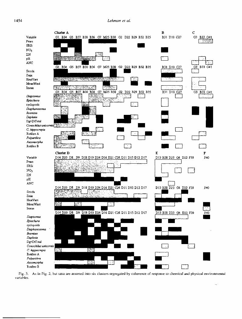
were treated as missing values. Euclidean distances were cal-culated among all pairwise contrasts. Taxa were then sortedinto clusters that exhibited minimal Euclidean distance dif-ferences among all members of the cluster. Finally, the clus-ters were inspected visually and were condensed to a set ofsix that displayed complete internal coherence with respectto both chemical and physical variables (Fig. 3).

Cluster A is dominated by four chlorophyte taxa and eightcyanophytes plus Mallomonas and Synedra tenera. Growthrates for these taxa are correlated positively (i.e., net growthis positive) with elevated lake heat, increased average lightin the mixed layer, increased pH, increased concentrationsof N species other than nitrate, and increasing abundancesof all copepods. Growth rates correlate negatively (i.e., netgrowth is negative) with increasing phosphorus, silica, ni-trate, water transparency, wind speeds, and mixed layerdepth. This is equivalent to saying that positive net growthis associated with decreasing P, Si, NO3, Secchi visibility,wind, and mixed layer thickness. The details of differencesamong the algal taxa trace entirely to idiosyncrasy of re-sponse to different Cladocera and rotifer taxa, with both pos-itive and negative responses common on a species-specificbasis.

Cluster B (B31, DIO, C27) is otherwise similar to clusterA except that the three taxa have growth rates that correlatepositively with water transparency. Cluster C (03, B33,041) differs further yet in that growth rates correlate posi-

tively with phosphorus, ANC, and wind speed, as well aswith water transparency.

Cluster D is dominated by 13 diatom taxa plus Chroom-onas minuta. These taxa are allied in exhibiting positivegrowth rates in response to elevated phosphorus, silica, ni-trate, water transparency, mixing depth, and wind speed.Their net growth rates are negatively affected by increasingepilimnion heat content, average light in the mixed layer,pH, and N species other than nitrate. Their net growth ratesare negatively associated, moreover, with elevated concen-trations of all copepods and Cladocera as well as most ro-tifers. This assemblage exhibits highly monolithic responseto chemical, physical, and biological variables.

Cluster E (gelatinous green algae, Fragilaria, Synedra te-nera, Anabaena, and Ceratium) differs from cluster D main-ly by exhibiting more positive responses to some zooplank-ton taxa, particularly Diaptomus. Some of the algal taxa incluster E also exhibit negative growth responses with in-creased water transparency and concentrations of ammonia.Cluster F (dinoflagellates other than Ceratium) does notclearly conform to any of the other clusters, and so it sitsalone.

The data do not permit resolution of statistically signifi-cant responses to all environmental variables for any of thealgal taxa, and so the matrix of responses is underdetermi-ned, causing some ambiguity of cluster assignments. Syne-dra tenera, for example, conforms with both cluster A and

Table 6. Chi-squared probabilities for tests of homogeneity between pairs of frequency distributions reported in Tables 4 and 5. "n.s."= not statistically significant at a = 0.05.

Diatoms Bluegreens Flagellates

Pos-r Neg-r Pos-r Neg-r Pos-r Neg-r

Greens 1.5X10-9 3.2X10- 4 n.s. n.s n.s. n.s.Diatoms 4.8x10-2 4.6xl0-23 0.0002 l.9X10-6Bluegreens 0.02 n.s.

1452

Phytoplankton growth in Lake Washington

Table 7. Chi-squared probabilities for tests of homogeneity be-tween frequency distributions for positive net growth rates and neg-ative net growth rates as reported in Tables 4 and 5.

Probability

All taxa 1.9X10-'4Greens 0.02Diatoms 2.9 x10 -47

Bluegreens 3.8x 10-8Flagellates n.s.

cluster E because the available data do not resolve its growthresponses to chemical variables (i.e., the contrasts betweenmean values of chemical variables during positive and neg-ative growth phases are statistically insignificant in all cas-es).

We assessed the degree to which clusters merely repre-sented taxa that exhibited contemporaneous correlationsamong abundances in situ. A correlation matrix was con-structed for all pairwise combinations of 40 algal taxa, usinglogarithm-transformed biovolumes. For each algal taxon, thecorrelation matrix was sorted to rank pairwise correlationsin decreasing order. For taxa belonging to clusters of size n,the top n - I correlations were surveyed to determine howmany other members of the same cluster numbered amongthe set of top-ranked correlations. This analysis was de-signed to test whether clusters represented species that tendto increase or decrease at the same time. The results weretested against expectations for hypergeometric distributionsdrawing on a population pool of 40 taxa and sampling thenumbers that appear in the clusters (Fig. 3). Results of thisanalysis are reported in Table 9. Of the 11 cases where clus-ter allies appear to exhibit contemporaneous correlations inbiovolume that are higher than by random assortment, 10are diatoms and all are from cluster D.

Response to physical variables-Algal divisions segregatewell by mixing depth during net positive growth (Fig. 4a)but not by water transparency per se (p = 0.16). Neither ofthe two physical variables in Fig. 4 segregate taxa at thedivision level when cells are in negative net growth phases(Fig. 4b). Both mixed layer temperature and mean irradiancein the mixed layer do, however, segregate the divisions wellduring both positive (Fig. Sa: p = 2 X 10 6 for Tmj; p =0.0004 for Imea) and negative (Fig. Sb: p = 0.007 for Tmixand p = 0.04 for I,,_) net growth rates.

Some statistically significant differences emerge at the di-vision level between the mean values of physical factorsassociated with positive and negative growth phases by two-

tailed paired t-test. Secchi transparency depth is different andhigher during positive growth for diatoms (p = 0.02) butlower during positive growth for bluegreens (p = 0.04).Mixing depth is also higher during positive growth for dia-toms (p = 0.004) and lower during positive growth for blue-greens (p = 0.006). Mixed layer temperatures are muchcooler (p = 0.0002) when diatoms are in positive growthphases than when in decline for every taxon except D1O(Cyclotella bodanica + C. comra), consistent with the dia-tom reputation for success at low light and low temperatures(Talling 1957; Will6n 1991). Mean light in the mixed layerwas slightly elevated overall during positive growth for di-atoms (p = 0.048), somewhat surprising in light of the ad-monition of Reynolds (1989) that the group is susceptible tophotoinhibition. Among the bluegreens, mixed layer lightintensities were generally lower during positive growth phas-es than negative ones (p = 0.004) for all taxa except Aphan-izomenon and Lyngbya.

Discussion

The community structure of phytoplankton in Lake Wash-ington appears to sort out remarkably well with environ-mental variables. There are two major modes of growth ratevariation in response to environmental conditions, with per-haps four additional variations on the major ones.

The most uniform growth response is one shared by mostof the diatom species (cluster D). These allied species riseand fall in unison. They prosper when nutrients are elevated,mixing is deep, and the water is both cold and transparent.They are impeded by thermal stratification and by increasingabundances of virtually any zooplankton species. There islittle qualitative in chemical, physical, or biological responsethat discriminates most of these species. The differencesamong taxa instead lie in the quantitative details of species-specific responses to resources, temperature, and light. Sy-nedra tenera is a notable exception to this pattern. The spe-cies enters the plankton as an epiphyte, and it seems to havebroken away from the typical diatom adaptive strategy.

A second major mode of growth response (cluster A) isexhibited by taxa endowed with motility or buoyancy. Thesespecies exploit nutrient-depleted and thermal stratified sur-face layers probably in part because as Reynolds (1983,1984a,b, 1989, 1994) has theorized insightfully, they are lossminimizers. These species have common responses to chem-ical and physical variables, but they differ in response tozooplankton. They generally benefit from increasing num-bers of copepods, but they exhibit species-specific responsesto Cladocera and rotifers. These taxa do not bloom or suc-

Table 8. Frequencies at which environmental variables aggregated by category are statistically significant during either positive ornegative growth phases by various taxon groupings.

Greens Diatoms Bluegreens Flagellates

Pos-r Neg-r Pos-r Neg-r Pos-r Neg-r Pos-r Neg-r

Chem vars 10 7 70 17 14 18 7 3Phys vars 12 5 29 35 23 13 7 4Zoop vars 28 15 14 181 66 18 7 15

1453

Lehman et al.

Cluster AVaiablePvarsSRSi

NO3

ENpHANC

SecchiZsnixHeatVarsMeanWindImean

DiaptomusEpischaracyclopoidsDiaphanosomaBosmifnaDaphniaDgfDtTotalConochbls umiconnsC. kippocrepisRobfers APoyarthraAscomorphaRotifers B

VariablePvarsSRSi

NO3

ZNpHANC

SecchZnixHeatVarsMeanWmdImean

DiapLomusEpzschuracyclopoidsDkaphanosomaBosmmaDaphniaDg+DtTotalConockilus umcormsC. hippocrmpsRotifers APohyar/raAscomorphaRotiftrs B

B30 B36 G7 M25 B38 G2 D22 B29 B32 B35

I~~~~ m

B30 B36 G7 M25 B38 G2 D22 B29 B32 B35

* m

ElElEi1

B30 B36 G7 M25 B38 G2 D22 B29 B32 B35

Chlster DD14 D20 D8 D9.'~" l . ...' , s I -..T.:

BB31 D10 C27

U

B31 D10 C27

1, I

B31 D10 C27

mOE

D18 D19 D24 D16 D21 C26 DII D15 D12 D17

D16 D21 C26 DII D15 D12 D17;~: I '

- mi,,Dlg D19 D24 D16 D21 C26 Dll D15 D12 D17

CG3 B33 041

G3 B33 041

G3 B33 041

m

FF39 F40

F40

LiJD13 B28 D23 G4 D22 F39 F40

OEl

.C=Fig. 3. As in Fig. 2, but taxa are assorted into six clusters segregated by coherence of response to chemical and physical environmental

variables.

1454

" � CD,, F-LLJ

Phytoplankton growth in Lake Washington

Table 9. Deviations of intertaxon biovolume correlations (Intransformation) from expected hypergeometric distributions withsample sizes set by the size of algal taxon clusters. "Correlations"= number of cluster allies that exhibit high contemporaneous cor-relation. "n.s." = the number of allied taxa with high correlationsdoes not exceed that expected by random sampling from the taxonpool.

GIGEGIGzGDGDDlDSD1DlDlDlDlDlDlIDlIDlIDID2DCDBDBDBDBDBCBCB

BEBE

B3B3B3BOB3-_B3_

B3132B3

F304

Taxon Cluster

AAC

4 E5 A

A8 D

D10 BI1I D12 D13 E14 D15 D16 D17 D18 D19 D20 D21 D22 A22 E23 E24 D25 A26 D27 B28 E29 A10 A31 B12 A33 C14 A35 A16 A17 A18 A9 E4i C

Correlations

43035388082

8723

108750228

70

4

l

0364631

p

n.s.n.s.n.s.

0.010n.s.n.s.

0.0100.010n.s.

0.010n.s.n.s.

0.0100.049n.s.n.s.

9.2x 10-0.0100.049

n.s.n.s.n.s.n.s.

0.010n.s.

0.049n.s.n.s.n.s.n.s.n.s.n.s.n.s.n.s.n.s.n.s.n.s.n.s.n.s.n.s.

ceed contemporaneously, but rather may exhibit differentialsuccesses in different years.

For clusters A, B, and C physical and chemical conditionsseem to set the stage for taxa that might succeed, but actualsuccess is governed by the constellation of grazers, partic-ularly cladoceran and rotifer grazers, that face the develop-ing populations. There appears to be high specificity to theways that individual grazers interact with individual algae inthese clusters. Differential and complementary effects ofcrustacean grazers on phytoplankton have been reported(Burns and Schallenberg 2001; Sommer et al. 2001). Thereare in fact several cases within clusters A, B, and C wherecopepods exhibit positive correlations with growth rate while

2

3

4

5

6

7C,0

a.N

4

5

6

7

a

A A

A

A

hAAa'A.* 0

oU

..

0

A

U

* U~n

b

a

mU *_

* U

A A*L A

A Aso

A A

* greens

5 A *A *diatomsA bluegreens

v 71 Mallomonaso cryptomonads

* dinoflagellates

0 5 1 0 15 20 25 30 35 40

Zmix (m)

45 50 55 60 65

Fig. 4. Mean values of mixed layer depth and Secchi transpar-ency depth during (a) positive or (b) negative net growth phases forLake Washington algal taxa.

various cladocerans exhibit negative correlations. However,the differences do not break out cleanly as large versus smallspecies as Sommer et al. report. Instead, the copepods arenegatively associated with the cluster D species (almost alldiatoms) and positively associated with most others. De-tailed specificity of grazer interaction with net algal growthrates traces mainly to the cladocerans and rotifers. Thosegrazers thus represent a biological gamut that selects a con-temporary species assemblage from a large pool of contend-ers.

It is noteworthy that a relatively few algal taxa exhibit nonegative net growth rate correlations with abundance of anyzooplankton taxon. These include Mallomonas (M25),Aphanizomenon (B29), Anacystis and its allies (B36),Aphanocapsa and its allies (B37), Lyngbya (B331), Oscilla-toria limnetica (B38), Ceratiumn (F39), and, surprisingly, Cy-clotella bodanica + C. comta (DIO) and Cryptomonas spp.(C27). Statistical power to detect differences for the Cyclo-tella species is weak because only two periods of sustaineddecline were identified in the entire data series. However, forCryptomonas the power is excellent, with over 200 dateseach of sustained increase or decrease. It is an empirical factin Lake Washington that the abundances of grazing zoo-plankton are no different on average between times of netincrease and net decrease for this taxon. For example, forall cases of positive net growth by Cryptomonas spp. whendetectable abundances of Daphnia spp. were present in the

1455

.

Lehman et al.

500 -

400 -

300

200

100

0 -

i 500-E

a

0

U

0 *

P . 00 A A

*: *z AU U

U

b* greens

*j~ AL

A

400 1 * diatoms

300 -

200

1oo

0-

A bluegreensD Mallomonas

o cryptomonads* dinoflagellates

5

a

Eu

U . * Z

A E 0 0

AIL AA A

A a A

10

* A0

A

15

Tmix (C)

Fig. 5. Mean values of mixed layer temperature and index ofmean irradiance in the mixed layer during (a) positive or (b) neg-ative net growth phases for Lake Washington algal taxa.

lake, the mean In abundance of Daphnia was 7.11 (SD -

2.37, n = 128); during net negative growth phases, In Daph-nia was 7.44 (SD = 2.16, n = 85).

The analysis documented in this report has a number ofadvantages for identifying environmental factors that arelinked with population dynamics of algal taxa.

1. The selection of growth criteria is well defined, objec-tive, and reproducible.

2. Environmental data that are extracted for analysis areconfidently assigned to episodes of either positive or nega-tive net growth.

3. Decisions about significance of effect are based on ap-plication of simple parametric statistics (e.g., t-test) to datathat exhibit normal frequency distributions.

4. Inferences about the importance of different environ-mental factors during positive and negative growth phasesare based on application of objective statistics to frequencydata.

Part of the reason that environmental conditions differ be-tween positive and negative growth phases for the variousspecies is certainly that the algae transform the chemical andoptical environment as they grow. They furthermore repre-sent a food resource that permits herbivorous zooplanktonto increase in abundance. The analysis presented here doesnot resolve the effects of the growing algae on environmen-tal variables. It looks at the environmental conditions during

growth and decline without attempting to explain how thedifferent conditions evolved. By identifying the key factorsassociated with increases and declines of algal taxa, the anal-ysis highlights variables that are most clearly related togrowth rates as well as the modalities by which they inter-play with the algae. This opens the way to subsequent anal-yses of the quantitative linkages among, for example, nutri-ent depletion or transparency declines and biomass accrual.

For example, the strongly negative associations betweenmost diatoms and virtually all zooplankton species could beregarded as a consequence of the fact that zooplankton tendto increase in Lake Washington during late spring as the lakewarms up and stratifies. This might threaten to be a case ofcorrelation without causal connection. However, zooplank-ton need to exploit food resources as they grow, and diatomsare likely candidates for exploitation. It is a fair question forfurther study whether the grazing potential of the zooplank-ton at ambient abundances is consistent with the rates ofdecline of diatom biovolume at key times now identified.

References

ANAGNOSTIDIs, K., AND J. KOMAREK. 1988. Modem approaches tothe classification system of cyanophytes. 3. Oscillatoriales.Arch. Hydrobiol. Suppl. 80: 327-472.

BURNS, C. W., AND M. SCHALLENBERG. 2001. Short-term impactsof nutrients, Daphnia, and copepods on microbial food-websof an oligotrophic and eutrophic lake. N. Z. J. Mar. FreshwaterRes. 35: 695-710.

EDMONDSON, W. T., S. E. B. ABELLA, AND J. T. LEHMAN. 2003.Phytoplankton in Lake Washington: Long-term changes 1950-1999. Arch. Hydrobiol. Suppl. 139: 1-52.

GRIME, J. P. 1979. Plant strategies and vegetation processes. Wiley.MARGALEF, R. 1978. Life-forms of phytoplankton as survival al-

ternatives in an unstable environment. Oceanol. Acta 1: 493-509.

REYNOLDS, C. S. 1983. A physiological interpretation of the dy-namic responses of populations of a planktonic diatom to phys-ical variability of the environment. New Phytol. 95: 41-53.

. 1984a. Phytoplankton periodicity: The interactions ofform, function and environmental variability. Freshwater Biol.14: 111-142.

______. 1984b. The ecology of freshwater phytoplankton. Cam-bridge Univ. Press.

-_____ 1988. Functional morphology and the adaptive strategiesof freshwater phytoplankton, pp. 388-433. In C. D. Sandgren[ed.], Growth and reproductive strategies of freshwater phy-toplankton. Cambridge Univ. Press.

_____. 1989. Physical determinants of phytoplankton succession,pp. 9-56. In U. Sommer [ed.], Plankton ecology. Springer.

- . 1994. The long, the short and the stalled: On the attributesof phytoplankton selected by physical mixing in lakes andstreams. Hydrobiologia 289: 9-21.

SOMMER, U., E SOMMER, B. SANTER, C. JAMIESON, M. BOERSMA,C. BECKER, AND T. HANSEN. 2001. Complementary impact ofcopepods and cladocerans on phytoplankton. Ecol. Lett. 4:545-550.

TALLING, J. E 1957. Photosynthetic characteristics of some fresh-water plankton diatoms in relation to underwater radiation.New Phytol. 56: 29-50.

WILLEN, E. 1991. Planktonic diatoms-an ecological review. Algol.Stud. 62: 69-106.

Received: 7 February 2003Accepted: 16 September 2003

Amended: 28 October 2003

1 456

COPYRIGHT INFORMATION

TITLE: Fingerprints of biocomplexity: Taxon-specific growth ofphytoplankton in relation to environmental factors

SOURCE: Limnol Oceanogr 49 no4 Jl 2004 pt2WN: 0418901853022

The magazine publisher is the copyright holder of this article and itis reproduced with permission. Further reproduction of this article inviolation of the copyright is prohibited. To contact the publisher:http://aslo.org/

Copyright 1982-2004 The H.W. Wilson Company. All rights reserved.