Finding Similar Items and Locality SensitiveHashing

STA 325, Supplemental Material

Andee Kaplan and Rebecca C. Steorts

1 / 84

Reading

The reading for this module can be found in Mining MassiveDatasets, Chapter 3.

http://infolab.stanford.edu/~ullman/mmds/book.pdf

There are no applied examples in the book, however, we will becovering these in class.

2 / 84

Libraries

library(knitr)

opts_chunk$set(message=FALSE, warning=FALSE)

# load librarieslibrary(rvest) # web scrapinglibrary(stringr) # string manipulationlibrary(dplyr) # data manipulationlibrary(tidyr) # tidy datalibrary(purrr) # functional programminglibrary(scales) # formatting for rmd outputlibrary(ggplot2) # plotslibrary(numbers) # divisors functionlibrary(textreuse) # detecting text reuse and# document similarity

3 / 84

Background

We first go through a bit of R programming that you have not seen.This will not be a complete review, so please be sure to go throughthis on your own after the lecture.

4 / 84

Piping

There is a helpful R trick (used in many other languages) known aspiping that we will use. Piping is available through R in themagrittr package and using the {%>%} command.

How does one use the pipe command? The pipe operator is used toinsert an argument into a function. The pipe operator takes theleft-hand side (LHS) of the pipe and uses it as the first argument ofthe function on the right-hand side (RHS) of the pipe.

5 / 84

Examples of Piping

We give two simple examples

# Example One1:50 %>% mean

## [1] 25.5

mean(1:50)

## [1] 25.5

6 / 84

Examples of Piping

# Example Twoyears <- factor(2008:2012)# nestingas.numeric(as.character(years))

## [1] 2008 2009 2010 2011 2012

# pipingyears %>% as.character %>% as.numeric

## [1] 2008 2009 2010 2011 2012

7 / 84

The dplyr package

A very useful function that I recommend that you explore and learnabout is called dplyr and there is a very good blogpost about itsfunctions: https://www.r-bloggers.com/useful-dplyr-functions-wexamples/

8 / 84

The dplyr package

Why should you learn and use dplyr?

I It will save you from writing your own complicated functions.I It’s also very useful as it will allow you to perform data

cleaning, manipulation, visualisation, and analysis.

9 / 84

The dplyr package

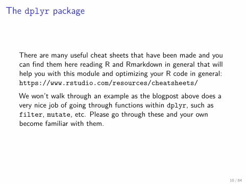
There are many useful cheat sheets that have been made and youcan find them here reading R and Rmarkdown in general that willhelp you with this module and optimizing your R code in general:https://www.rstudio.com/resources/cheatsheets/

We won’t walk through an example as the blogpost above does avery nice job of going through functions within dplyr, such asfilter, mutate, etc. Please go through these and your ownbecome familiar with them.

10 / 84

Information Retrieval

One of the fundamental problems with having a lot of data isfinding what you’re looking for.

This is called information retrieval!

In this module, we will look at the problem of how to examine datafor similar items for very large data sets.

11 / 84

Finding Similar Items

Suppose that we have a collection of webpages and we wish to findnear-duplicate pages. (We might be looking for plagarism).

We will introduce how the problem of finding textually similardocuments can be turned into a set using a method called shingling.

Then, we will introduce a concept called minhashing, whichcompresses large sets in such a way that we can deduce thesimilarity of the underlying sets from their compressed versions.

Finally, we will discuss an important problem that arises when wesearch for similar items of any kind, there can be too many pairs ofitems to test each pair for their degree of similarity. This concernmotivates locality sensitive hashing, which focuses our search onpairs that are most likely to be similar.

12 / 84

Notions of Similarity

We have already discussed many notions of similarity, however, themain one that we work with in this module is the Jaccard similarity.

The Jaccard similarity of set S and T is

|S ∩ T ||S ∪ T |

.

We will refer to the Jaccard similarity of S and T by SIM(S,T ).

13 / 84

Jaccard Similarity

Figure 1: Two sets S and T with Jaccard similarity 2/5. The two setsshare two elements in common, and there are five elements in total.

14 / 84

Shingling of Documents

The most effective way to represent document as sets is to constructfrom the document the set of short strings that appear within it.

Then the documents that share pieces as short strings will havemany common elements.

Here, we introduce the most simple and common approach —shingling.

15 / 84

k-Shingles

A document can be represented as a string of characters.

We define a k-shingle (k-gram) for a document to be any sub-stringof length k found within the document.

Then we can associate with each document the set of k-shinglesthat appear one or more times within the document.

16 / 84

k-Shingles

Example: Suppose our document is the string abcdabd and k = 2.

The set of 2-shingles is {ab, bc, cd , da, bd}.

Note the sub-string ab appears twice within the document but onlyonce as a shingle.

Note it also makes sense to replace any sequence of one or morewhite space characters by a single blank. We can then distinguishshingles that cover two or more words from those that do not.

17 / 84

Choosing the shingle size

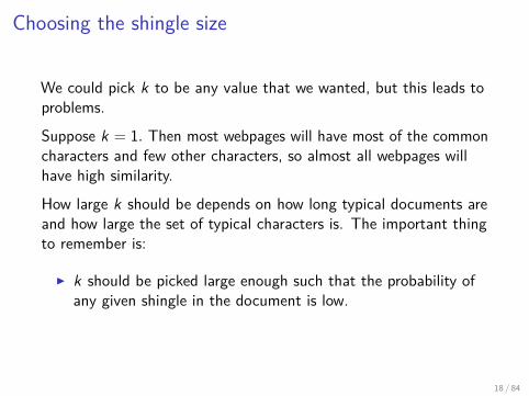
We could pick k to be any value that we wanted, but this leads toproblems.

Suppose k = 1. Then most webpages will have most of the commoncharacters and few other characters, so almost all webpages willhave high similarity.

How large k should be depends on how long typical documents areand how large the set of typical characters is. The important thingto remember is:

I k should be picked large enough such that the probability ofany given shingle in the document is low.

18 / 84

Choosing the shingle size

For example, if our corpus of documents is emails, then k=5, shouldbe fine. Why?

Suppose that only letters and general white space characters appearin emails.

If so, there would be 275 = 14, 348, 907 possible shingles.

Since the typical email is much smaller than 14 million characterslong, we would expect k = 5 to work well and it does.

19 / 84

Choosing the shingle size

Surely, more than 27 characters appear in emails!

However, not all characters appear with equal probability.

Common letters and blanks dominate, while “z” and other lettersthat have high point values in Scrabble are rare.

Thus, even short emails will have many 5-shingles consisting ofcommon letters and the chances of unrelated emails sharing thesecommon shingles is greater than implied by the previous calculation.

A rule of thumb is to imagine there are 20 characters and estimatethe number of shingles as 20k . For large documents (researcharticles), a choice of k = 9 is considered to be safe.

20 / 84

Jaccard similarity of Beatles songs

Now that we have shingled records (sets), we can now look at theJaccard similarity for each song by looking at the shingles for eachsong as a set (Si) and computing the Jaccard similarity

|Si ∩ Sj ||Si ∪ Sj |

for i 6= j .

We will use textreuse::jaccard_similarity() to performthese computations.

21 / 84

DataWe will scrape lyrics from http://www.metrolyrics.com. (Pleasenote that I do not expect you to be able to scrape the data, but thecode is on the next two slides in case you are interested in it.)

# get beatles lyricslinks <- read_html("http://www.metrolyrics.com/beatles-lyrics.html") %>% # lyrics site

html_nodes("td a") # get all links to all songs

# get all the links to song lyricstibble(name = links %>% html_text(trim = TRUE) %>% str_replace(" Lyrics", ""), # get song names

url = links %>% html_attr("href")) -> songs # get links

# function to extract lyric text from individual sitesget_lyrics <- function(url){

test <- try(url %>% read_html(), silent=T)if ("try-error" %in% class(test)) {

# if you can't go to the link, return NAreturn(NA)

} elseurl %>% read_html() %>%

html_nodes(".verse") %>% # this is the texthtml_text() -> words

words %>%paste(collapse = ' ') %>% # paste all paragraphs together as one string

str_replace_all("[\r\n]" , ". ") %>% # remove newline charsreturn()

}

22 / 84

Data (continued)

# get all the lyrics# remove duplicates and broken linkssongs %>%

mutate(lyrics = (map_chr(url, get_lyrics))) %>%filter(nchar(lyrics) > 0) %>% #remove broken linksgroup_by(name) %>%mutate(num_copy = n()) %>%# remove exact duplicates (by name)filter(num_copy == 1) %>%select(-num_copy) -> songs

We end up with the lyrics to 62 Beatles songs and we can start tothink about how to first represent the songs as collections of shortstrings (shingling). As an example, let’s shingle the best Beatles’song of all time, “Eleanor Rigby”.

23 / 84

Back to the Beatles

I How would we create a set of k-shingles for the song “EleanorRigby”?

I We want to construct from the lyrics the set of short stringsthat appear within it.

I Then the songs that share pieces as short strings will havemany common elements.

I We will get the k-shingles (sub-string of length k words foundwithin the document) for “Eleanor Rigby” using the functiontextreuse::tokenize_ngrams().

24 / 84

Shingling Eleanor Rigby# get k = 5 shingles for "Eleanor Rigby"# this song is the best# filter finds when cases are truebest_song <- songs %>% filter(name == "Eleanor Rigby")# shingle the lyricsshingles <- tokenize_ngrams(best_song$lyrics, n = 5)

# inspect resultshead(shingles) %>%

kable() # pretty table

ah look at all thelook at all the lonelyat all the lonely peopleall the lonely people ahthe lonely people ah looklonely people ah look at

25 / 84

Shingling Eleanor Rigby

# get k = 3 shingles for "Eleanor Rigby"shingles <- tokenize_ngrams(best_song$lyrics, n = 3)

# inspect resultshead(shingles) %>%

kable()

ah look atlook at allat all theall the lonelythe lonely peoplelonely people ah

26 / 84

Shingling Eleanor Rigby

I We looked at k = 3 and k = 5 but what should k be?I How large k should be depends on how long typical songs are.I The important thing to remember is k should be picked large

enough such that the probability of any given shingle in thedocument is low.

I For simplicity, I will assume k = 3.

(For more on how to optimally pick k, seehttps://arxiv.org/abs/1510.07714)

27 / 84

Shingling all Beatles songs

We can now apply the shingling to all 62 Beatles songs in ourcorpus.

# add shingles to each song# map applies a function to each elt, returns vector# mutate adds new variables and preserves existingsongs %>%

mutate(shingles = (map(lyrics, tokenize_ngrams, n = 3))) -> songs

28 / 84

Shingling all Beatles songs

Again, you should think about the optimal choice of k here.

How would you do this? This is an exercise to think about on yourown. (Hints: Can you actually evaluate k here. Think about therecall. Can you compute the recall? Why or why not?)

29 / 84

Jaccard similarity of Beatles songs

# create all pairs to compare then get the jacard similarity of each# start by first getting all possible combinationssong_sim <- expand.grid(song1 = seq_len(nrow(songs)), song2 = seq_len(nrow(songs))) %>%

filter(song1 < song2) %>% # don't need to compare the same things twicegroup_by(song1, song2) %>% # converts to a grouped tablemutate(jaccard_sim = jaccard_similarity(songs$shingles[song1][[1]],

songs$shingles[song2][[1]])) %>%ungroup() %>% # Undoes the groupingmutate(song1 = songs$name[song1],

song2 = songs$name[song2]) # store the names, not "id"

# inspect resultssummary(song_sim)

## song1 song2 jaccard_sim## Length:1891 Length:1891 Min. :0.000000## Class :character Class :character 1st Qu.:0.000000## Mode :character Mode :character Median :0.000000## Mean :0.002021## 3rd Qu.:0.000000## Max. :0.982353

30 / 84

Jaccard similarity of Beatles songs

A Day In The Life

A Hard Day's Night

Abbey Road Medley

Across The Universe

All My Loving

All Together Now

All You Need is Love

And I Love Her

Bad To Me

Because

Birthday

Come Together

Dear Prudence

Dig a Pony

Eight Days a Week

Eleanor Rigby

For No One

Get Back

Girl

Golden Slumbers

Golden Slumbers/Carry That Wieght/Ending

Good Day Sunshine

Help

Here, There And Everywhere

I Am The Walrus

I Saw Her Standing There

I Will

I'm So Tired

I've Got A Feeling

I've Just Seen A Face

If I Fell

Imagine

Lady Madonna

Love Me Do

Lucy In The Sky With Diamonds

Maxwell's Silver Hammer

Michelle

Norwegian Wood

Nowhere Man

Obladi Oblada

Octopus's Garden

Penny Lane

Please Please Me

Revolution

Rocky Raccoon

Sgt. Pepper's Lonely Hearts Club Band

She Came In Through The Bathroom Window

She Loves You

She's Leaving Home

Something

Strawberry Fields Forever

The End

There are places I remember

Ticket To Ride

Two Of Us

We Can Work It Out

When I'm 64

When I'm Sixty−four

While My Guitar Gently Weeps

With A Little Help From My Friends

Yellow Submarine

A D

ay In

The

Life

A H

ard

Day

's N

ight

Abb

ey R

oad

Med

ley

Acr

oss

The

Uni

vers

e

All

My

Lovi

ng

All

Toge

ther

Now

All

You

Nee

d is

Lov

e

And

I Lo

ve H

er

Bad

To

Me

Bec

ause

Bir

thda

y

Com

e To

geth

er

Dea

r P

rude

nce

Dig

a P

ony

Eig

ht D

ays

a W

eek

Ele

anor

Rig

by

For

No

One

Get

Bac

k

Girl

Gol

den

Slu

mbe

rs

Gol

den

Slu

mbe

rs/C

arry

Tha

t Wie

ght/E

ndin

g

Goo

d D

ay S

unsh

ine

Hel

p

Her

e, T

here

And

Eve

ryw

here

I Am

The

Wal

rus

I Saw

Her

Sta

ndin

g T

here

I Will

I'm S

o T

ired

I've

Got

A F

eelin

g

I've

Just

See

n A

Fac

e

If I F

ell

Imag

ine

In M

y Li

fe

Lady

Mad

onna

Love

Me

Do

Lucy

In T

he S

ky W

ith D

iam

onds

Max

wel

l's S

ilver

Ham

mer

Mic

helle

Nor

weg

ian

Woo

d

Now

here

Man

Obl

adi O

blad

a

Oct

opus

's G

arde

n

Pen

ny L

ane

Ple

ase

Ple

ase

Me

Rev

olut

ion

Roc

ky R

acco

on

Sgt

. Pep

per's

Lon

ely

Hea

rts

Clu

b B

and

She

Cam

e In

Thr

ough

The

Bat

hroo

m W

indo

w

She

Lov

es Y

ou

She

's L

eavi

ng H

ome

Str

awbe

rry

Fie

lds

For

ever

The

End

The

re a

re p

lace

s I r

emem

ber

Tic

ket T

o R

ide

Two

Of U

s

We

Can

Wor

k It

Out

Whe

n I'm

64

Whe

n I'm

Six

ty−

four

Whi

le M

y G

uita

r G

ently

Wee

ps

With

A L

ittle

Hel

p F

rom

My

Frie

nds

Yello

w S

ubm

arin

esong1

song

2

0.00

0.25

0.50

0.75

jaccard_sim

It looks like there are a couple song pairings with very high Jaccard similarity. Let’s filter to find out which ones.

31 / 84

Jaccard similarity of Beatles songs

# filter high similarity pairssong_sim %>%

filter(jaccard_sim > .5) %>% # only look at those with similarity > .5kable() # pretty table

song1 song2 jaccard_sim

In My Life There are places I remember 0.6875000When I’m 64 When I’m Sixty-four 0.9823529

Two of the three matches seem to be from duplicate songs in the data, although it’s interesting that their Jaccardsimilarity coefficients are not equal to 1. (This is not suprising. Why?). Perhaps these are different versions of thesong.

32 / 84

Jaccard similarity of Beatles songs

# inspect lyricsprint(songs$lyrics[songs$name == "In My Life"])

## [1] "There are places I remember. All my life though some have changed. Some forever not for better. Some have gone and some remain. All these places have their moments. With lovers and friends I still can recall. Some are dead and some are living. In my life I've loved them all But of all these friends and lovers. There is no one compares with you. And these memories lose their meaning. When I think of love as something new. Though I know I'll never lose affection. For people and things that went before. I know I'll often stop and think about them. In my life I love you more Though I know I'll never lose affection. For people and things that went before. I know I'll often stop and think about them. In my life I love you more In my life I love you more"

print(songs$lyrics[songs$name == "There are places I remember"])

## [1] "There are places I remember all my life. Though some have changed. Some forever, not for better. Some have gone and some remain All these places have their moments. Of lovers and friends I still can recall. Some are dead and some are living. In my life I loved them all And with all these friends and lovers. There is no one compares with you. And these mem'ries lose their meaning. When I think of love as something new And I know I'll never lose affection. For people and things that went before. I know I'll often stop and think about them. In my life I loved you more And I know I'll never lose affection. For people and things that went before. I know I'll often stop and think about them. In my life I loved you more. In my life I loved you more"

By looking at the seemingly different pair of songs lyrics, we can see that these are actually the same song as well,but with slightly different transcription of the lyrics. Thus we have identified three songs that have duplicates inour database by using the Jaccard similarity. What about non-duplicates? Of these, which is the most similar pairof songs?

33 / 84

Jaccard dissimilarity of Beatles songs

# filter to find the songs that aren't very similar# These are songs that we don't want to look atsong_sim %>%

filter(jaccard_sim <= .5) %>%arrange(desc(jaccard_sim)) %>% # sort by similarityhead() %>%kable()

song1 song2 jaccard_sim

Golden Slumbers/Carry That Wieght/Ending Golden Slumbers 0.3557692Golden Slumbers/Carry That Wieght/Ending The End 0.2616822Golden Slumbers/Carry That Wieght/Ending Abbey Road Medley 0.1583333Abbey Road Medley She Came In Through The Bathroom Window 0.1458671Golden Slumbers Abbey Road Medley 0.0626058The End Abbey Road Medley 0.0418760

These appear to not be the same songs, and hence, we don’t want to look at these. Typically our goal is to look atitems that are most similar and discard items that aren’t similar.

34 / 84

Jaccard similarity of Beatles songs

Note, although we computed these pairwise comparisons manually,there is a set of functions that could have helped —textreuse::TextReuseCorpus(),textreuse::pairwise_compare() andtextreuse::pairwise_candidates().

Think about how you would do this and investigate this on yourown (Exercise).

35 / 84

Solution to Exercise (Go over on your own)

# build the corpus using textreusedocs <- songs$lyricsnames(docs) <- songs$name # named vector for document idscorpus <- TextReuseCorpus(text = docs,

tokenizer = tokenize_ngrams, n = 3,progress = FALSE,keep_tokens = TRUE)

36 / 84

Solution to Exercise (Go over on your own)

# create the comparisonscomparisons <- pairwise_compare(corpus, jaccard_similarity, progress = FALSE)comparisons[1:3, 1:3]

## In My Life All You Need is Love## In My Life NA 0## All You Need is Love NA NA## There are places I remember NA NA## There are places I remember## In My Life 0.6875## All You Need is Love 0.0000## There are places I remember NA

37 / 84

Solution to Exercise (Go over on your own)

# look at only those comparisons with Jaccard similarity > .1candidates <- pairwise_candidates(comparisons)candidates[candidates$score > 0.1, ] %>% kable()

a b score

Abbey Road Medley Golden Slumbers/Carry That Wieght/Ending 0.1583333Abbey Road Medley She Came In Through The Bathroom Window 0.1458671Golden Slumbers Golden Slumbers/Carry That Wieght/Ending 0.3557692Golden Slumbers/Carry That Wieght/Ending The End 0.2616822In My Life There are places I remember 0.6875000When I’m 64 When I’m Sixty-four 0.9823529

38 / 84

Jaccard similarity of Beatles songs

For a corpus of size n, the number of comparisons we must computeis n2−n

2 , so for our set of songs, we needed to compute 1, 891comparisons. This was doable for such a small set of documents, butif we were to perform this on the full number of Beatles songs (409songs recorded), we would need to do 83, 436 comparisons. As youcan see, for a corpus of any real size this becomes infeasible quickly.A better approach for corpora of any realistic size is to use hashing.

The textreuse::TextReuseCorpus() function hashes ourshingled lyrics automatically using function that hashes a string toan integer. We can look at these hashes for “Eleanor Rigby”.

Before we do this, let’s talk about what hashing is and why it’suseful!

39 / 84

Hashing

I Traditionally in computer science, a hash function will mapobjects to integers such that similar objects are far apart.

I We’re going to look at special hash functions that do theopposite of this.

I Specifically, we’re going to look at hash functions where similarobjects are placed closed together!

Formally these hash functions h() are defined such that

I if SIM(A,B) is high, then with high probability h(A) = h(B).I if SIM(A,B) is low, then with high probability h(A) 6= h(B).

40 / 84

Hashing shingles

Instead of using substrings as shingles, we can use a hash function,which maps strings of length k to some number of buckets andtreats the resulting bucket number as the shingle.

The set representing a document is then the set of integers of oneor more k-shingles that appear in the document.

Example: We could construct the set of 9-shingles for a document.We could then map the set of 9-shingles to a bucket number in therange 0 to 232 − 1.

Thus, each shingle is represented by four bytes intead of 9. Thedata has been compressed and we can now manipulate (hashed)shingles by single-word machine operations.

41 / 84

Similarity Preserving Summaries of Sets

Sets of shingles are large. Even if we hash them to four bytes each,the space needed to store a set is still roughly four times the spacetaken up by the document.

If we have millions of documents, it may not be possible to store allthe shingle-sets in memory. (There is another more serious problem,which we will address later in the module.)

Here, we replace large sets by smaller representations, calledsignatures. The important property we need for signatures is thatwe can compare the signatures of two sets and estimate the Jaccardsimilarity of the underlying sets from the signatures alone.

It is not possible for the signatures to give the exact similarity of thesets they represent, but the estimates they provide are close.

42 / 84

Characteristic MatrixBefore describing how to construct small signatures from large sets,we visualize a collection of sets as a characteristic matrix.The columns correspond to sets and the rows correspond to theuniversal set from which the elements are drawn.There is a 1 in row r, column c if the element for row r is a memberof the set for column c. Otherwise, the value for (r , c) is 0.Below is an example of a characteristic matrix, with four shinglesand five records.

library("pander")element <- c("a","b","c","d","e")S1 <- c(0,1,1,0,1)S2 <- c(0,0,1,0,0)S3 <- c(1,0,0,0,0)S4 <- c(1,1,0,1,1)my.data <- cbind(element,S1,S2,S3,S4)

43 / 84

Characteristic Matrix

pandoc.table(my.data,style="rmarkdown")

###### | element | S1 | S2 | S3 | S4 |## |:-------:|:--:|:--:|:--:|:--:|## | a | 0 | 0 | 1 | 1 |## | b | 1 | 0 | 0 | 1 |## | c | 1 | 1 | 0 | 0 |## | d | 0 | 0 | 0 | 1 |## | e | 1 | 0 | 0 | 1 |

Why would we not store the data as a characteristic matrix (thinksparsity)?

44 / 84

Minhashing

The signatures we desire to construct for sets are composed of theresults of a large number of calculations, say several hundred, eachof which is a “minhash” of the characteristic matrix.

Here, we will learn how to compute the minhash in principle. Later,we will learn how a good approximation is computed in practice.

To minhash a set represented by a column of the characteristicmatrix, pick a permutation of the rows.

The minhash value of any column is the index of the first row in thepermuted order in which the column has a 1.

45 / 84

MinhashingNow, we permute the rows of the characteristic matrix to form apermuted matrix.The permuted matrix is simply a reordering of the originalcharacteristic matrix, with the rows swapped in some arrangement.Figure 2 shows the characteristic matrix converted to a permutedmatrix by a given permutation. We repeat the permutation step forseveral iterations to obtain multiple permuted matrices.

Figure 2: Permuted matrix from the characteristic one. The π vector isthe specified permutation.

46 / 84

The Signature Matrix

Now, we compute the signature matrix.

The signature matrix is a hashing of values from the permuted one.

The signature has a row for the number of permutations calculated,and a column corresponding with the columns of the permutedmatrix.

We iterate over each column of the permuted matrix, and populatethe signature matrix, row-wise, with the row index from the first 1value found in the column.

47 / 84

Signature Matrix

library("pander")signature <- c(2,4,3,1)pandoc.table(signature,style="rmarkdown")

#### | | | | |## |:-:|:-:|:-:|:-:|## | 2 | 4 | 3 | 1 |

48 / 84

Minhashing and Jaccard Similarity

Based on the results of the signature matrix, we observe the pairwisesimilarity of two records. For the number of hash functions, there isan interesting relationship that we use between the columns for anygiven set of the signature matrix and a Jaccard Similarity measure.

49 / 84

Minhashing and Jaccard SimilarityThe relationship between the random permutations of thecharacteristic matrix and the Jaccard Similarity is:

Pr{min[h(A)] = min[h(B)]} = |A ∩ B||A ∪ B|

The equation means that the probability that the minimum valuesof the given hash function, in this case h, is the same for sets A andB is equivalent to the Jaccard Similarity, especially as the number ofrecord comparisons increases.

We use this relationship to calculate the similarity between any tworecords.

We look down each column, and compare it to any other column:the number of agreements over the total number of combinations isequal to Jaccard measure.

50 / 84

Back to the Beatles

Recall that textreuse::TextReuseCorpus() function hashes ourshingled lyrics automatically using function that hashes a string toan integer. We can look at these hashes for “Eleanor Rigby”.

# look at the hashed shingles for "Eleanor Rigby"tokens(corpus)$`Eleanor Rigby` %>% head()

## [1] "ah look at" "look at all" "at all the"## [4] "all the lonely" "the lonely people" "lonely people ah"

hashes(corpus)$`Eleanor Rigby` %>% head()

## [1] -1188528426 1212580251 2071766612 -964323450 -614667204 -153136944

51 / 84

Back to the Beatles

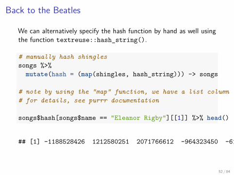
We can alternatively specify the hash function by hand as well usingthe function textreuse::hash_string().

# manually hash shinglessongs %>%

mutate(hash = (map(shingles, hash_string))) -> songs

# note by using the "map" function, we have a list column# for details, see purrr documentation

songs$hash[songs$name == "Eleanor Rigby"][[1]] %>% head()

## [1] -1188528426 1212580251 2071766612 -964323450 -614667204 -153136944

52 / 84

Back to the Beatles

Now instead of storing the strings (shingles), we can just store thehashed values. Since these are integers, they will take less spacewhich will be useful if we have large documents. Instead ofperforming the pairwise Jaccard similarities on the strings, we canperform them on the hashes.# compute jaccard similarity on hashes instead of shingled lyrics# add this column to our song data.framesong_sim %>%

group_by(song1, song2) %>%mutate(jaccard_sim_hash =

jaccard_similarity(songs$hash[songs$name == song1][[1]],songs$hash[songs$name == song2][[1]])) -> song_sim

# how many songs do the jaccard similarity computed from hashing# versus the actual shingles NOT match?sum(song_sim$jaccard_sim != song_sim$jaccard_sim_hash)

## [1] 0

53 / 84

Back to the Beatles

I We can start by visualizing our collection of sets as acharacteristic matrix where the columns correspond to songsand the rows correspond to all of the possible shingledelements in all songs.

I There is a 1 in row r , column c if the shingled phrase for row ris in the song corresponding to column c.

I Otherwise, the value for (r , c) is 0.

54 / 84

Characterisitic Matrix for the Beatles# return if an item is in a listitem_in_list <- function(item, list) {

as.integer(item %in% list)}

# get the characteristic matrix# items are all the unique hash values# lists will be each song# we want to keep track of where each hash is includeddata.frame(item = unique(unlist(songs$hash))) %>%

group_by(item) %>%mutate(list = list(songs$name)) %>% # include the song name for each itemunnest(list) %>% # expand the list column out# record if item in listmutate(included = (map2_int(item, songs$hash[songs$name == list], item_in_list))) %>%spread(list, included) -> char_matrix # tall data -> wide data (see tidyr documentation)

# inspect resultschar_matrix[1:4, 1:4] %>%

kable()

item A Day In The Life A Hard Day’s Night Abbey Road Medley

-2147299362 0 0 0-2147099044 0 0 0-2146305897 0 0 0-2145853136 0 0 0

55 / 84

Characterisitic Matrix for the Beatles

As you can see (and imagine), this matrix tends to be sparsebecause the set of unique shingles across all documents will be fairlylarge. Instead we want create the signature matrix throughminhashing which will give us an approximation to measure thesimilarity between song lyrics.

56 / 84

Signature Matrix for the Beatles

To compute the signature matrix, we first permute the characteristicmatrix and then iterate over each column of the permuted matrixand populate the signature matrix, row-wise, with the row indexfrom the first 1 value found in the column.

The signature matrix is a hashing of values from the permuted oneand has a row for the number of permutations calculated, and acolumn corresponding with the columns of the permuted matrix.We can show this for the first permutation.

57 / 84

Signature Matrix for the Beatles# set seed for reproducibilityset.seed(09142017)

# get permutation orderpermute_order <- sample(seq_len(nrow(char_matrix)))

# get min location of "1" for each column (apply(2, ...))sig_matrix <- char_matrix[permute_order, -1] %>%

apply(2, function(col) min(which(col == 1))) %>%as.matrix() %>% t()

# inspect resultssig_matrix[1, 1:4] %>% kable()

A Day In The Life 28A Hard Day’s Night 87Abbey Road Medley 6Across The Universe 63 58 / 84

Signature Matrix for the BeatlesWe can now repeat this process many times to get the full signaturematrix.# function to get signature for 1 permutationget_sig <- function(char_matrix) {

# get permutation orderpermute_order <- sample(seq_len(nrow(char_matrix)))

# get min location of "1" for each column (apply(2, ...))char_matrix[permute_order, -1] %>%

apply(2, function(col) min(which(col == 1))) %>%as.matrix() %>% t()

}

# repeat many timesm <- 360for(i in 1:(m - 1)) {

sig_matrix <- rbind(sig_matrix, get_sig(char_matrix))}

# inspect resultssig_matrix[1:4, 1:4] %>% kable()

A Day In The Life A Hard Day’s Night Abbey Road Medley Across The Universe

28 87 6 6370 30 4 983 181 21 20

42 23 5 25

59 / 84

Signature Matrix, Jaccard Similarity, and the Beatles

Since we know the relationship between the random permutations ofthe characteristic matrix and the Jaccard Similarity is

Pr{min[h(A)] = min[h(B)]} = |A ∩ B||A ∪ B|

we can use this relationship to calculate the similarity between anytwo records. We look down each column of the signature matrix,and compare it to any other column. The number of agreementsover the total number of combinations is an approximation toJaccard measure.

60 / 84

Signature Matrix, Jaccard Similarity, and the Beatles

# add jaccard similarity approximated from the minhash to compare# number of agreements over the total number of combinationssong_sim <- song_sim %>%

group_by(song1, song2) %>%mutate(jaccard_sim_minhash =

sum(sig_matrix[, song1] == sig_matrix[, song2])/nrow(sig_matrix))

# how far off is this approximation?summary(abs(song_sim$jaccard_sim_minhash - song_sim$jaccard_sim))

## Min. 1st Qu. Median Mean 3rd Qu. Max.## 0.0000000 0.0000000 0.0000000 0.0003798 0.0000000 0.0224359

61 / 84

Evaluating Performance

Suppose that we wish to evaluate the performance of how well ourmethod works in practice.

We would require some training data (hand-matched data) on theBeatles songs such that we could compute the recall and precision.

62 / 84

Evaluating Performance

Our first step would be either accessing or creating pairs of songsand noting whether these songs are a match or a non-match.

We would want to store this into a data set so that we could use itlater if needed (and would not need to repeat our results).

How would you go about doing this?

63 / 84

Evaluating Performance

Once you have a handmatched data set, we can calculate the recalland the precision.

How do we calculate the recall and precision?

We need to learn some new terminology first and then we’re all set!

64 / 84

Classifications1. Pairs of data can be linked in both the handmatched training

data (which we refer to as ‘truth’) and under the estimatedlinked data. We refer to this situation as true positives (TP).

2. Pairs of data can be linked under the truth but not linkedunder the estimate, which are called false negatives (FN).

3. Pairs of data can be not linked under the truth but linkedunder the estimate, which are called false positives (FP).

4. Pairs of data can be not linked under the truth and also notlinked under the estimate, which we refer to as true negatives(TN).

Then the true number of links is TP + FN, while the estimatednumber of links is TP + FP. The usual definitions of false negativerate and false positive rate are

FNR = FN/(TP+FN)FPR = FP/(TP+FP)

65 / 84

Classifications

FNR = FN/(TP+FN)

FPR = FP/(TP+FP)

Thenrecall = 1− FNR.

precision = 1− FPR.

How would you look at the sensitivity of a method for the recallandd the precision?

66 / 84

Signature Matrix, Jaccard Similarity, and the Beatles

While we have used minhashing to get an approximation to theJaccard similarity, which helps by allowing us to store less data(hashing) and avoid storing sparse data (signature matrix), we stillhaven’t addressed the issue of pairwise comparisons.

This is where locality-sensitive hashing (LSH) can help.

67 / 84

General idea of LSH

Our general approach to LSH is to hash items several times suchthat similar items are more likely to be hashed into the same bucket(bin).

68 / 84

Candidate Pairs

Any pair that is hashed to the same bucket for any hashings iscalled a candidate pair.

We only check candidate pairs for similarity.

The hope is that most of the dissimilar pairs will never hash to thesame bucket (and never be checked).

69 / 84

False Negative and False Positives

Dissimilar pairs that are hashed to the same bucket are called falsepositives.

We hope that most of the truly similar pairs will hash to the samebucket under at least one of the hash functions.

Those that don’t are called false negatives.

70 / 84

How to choose the hashings

Suppose we have minhash signatures for the items.

Then an effective way to choose the hashings is to divide up thesignature matrix into b bands with r rows.

For each band b, there is a hash function that takes vectors of rintegers (the portion of one column within that band) and hashesthem to some large number of buckets.

We can use the same hash function for all the bands, but we use aseparate bucket array for each band, so columns with the samevector in different bands will hash to the same bucket.

71 / 84

Example

Consider the signature matrix

The second and fourth columns each have a column vector [0, 2, 1]in the first band, so they will be mapped to the same bucket in thehashing for the first band.

Regardless of the other columns in the other bands, this pair ofcolumns will be a candidate pair.

72 / 84

Example (continued)

It’s possible that other columns such as the first two will hash to thesame bucket according to the hashing in the first band.

But their column vectors are different, [1, 3, 0] and [0, 2, 1] andthere are many buckets for each hashing, so an accidential collisionhere is thought to be small.

73 / 84

Analysis of the banding technique

You can learn some about the analysis of the banding technique onyour own in Mining Massive Datasets, Ch 3, 3.4.2.

74 / 84

Combining the Techniques

We can now give an approach to find the set of candidate pairs for similar documents and then find similardocuments among these.

1. Pick a value k and construct from each document the set of k-shingles. (Optionally, hash the k-shingles toshorter bucket numbers).

2. Sort the document-shingle pairs to order them by shingle.3. Pick a length n for the minhash signatures. Feed the sorted list to the algorithm to compute the minhash

signatures for all the documents.4. Choose a threshold t that defines how similar doucments have to be in order to be regarded a similar pair.

Pick a number b bands and r rows such that br = n and then the threshold is approximately (1/b)1/r .

5. Construct candidate pairs by applying LSH.6. Examine each candidate pair’s signatures and determine whether the fraction of components they agree is

at least t.7. Optionally, if the signatures are sufficiently similar, go to the documents themselves and check that they

are truly similar.

75 / 84

LSH for the Beatles

I Recall, performing pairwise comparisons in a corpus istime-consuming because the number of comparisons grows atO(n2).

I Most of those comparisons, furthermore, are unnecessarybecause they do not result in matches due to sparsity.

I We will use the combination of minhash and locality-sensitivehashing (LSH) to solve these problems. They make it possibleto compute possible matches only once for each document, sothat the cost of computation grows linearly.

76 / 84

LSH for the BeatlesWe want to hash items several times such that similar items aremore likely to be hashed into the same bucket. Any pair that ishashed to the same bucket for any hashing is called a candidate pairand we only check candidate pairs for similarity.

1. Divide up the signature matrix into b bands with r rows suchthat m = b ∗ r where m is the number of times that we drew apermutation of the characteristic matrix in the process ofminhashing (number of rows in the signature matrix).

2. Each band is hashed to a bucket by comparing the minhash forthose permutations. If they match within the band, then theywill be hashed to the same bucket.

3. If two documents are hashed to the same bucket they will beconsidered candidate pairs. Each pair of documents has asmany chances to be considered a candidate as there are bands,and the fewer rows there are in each band, the more likely it isthat each document will match another.

77 / 84

Choosing b?

I The question becomes, how to choose b, the number of bands?I We now it must divide m evenly such that there are the same

number of rows r in each band, but beyond that we need moreguidance.

I We can estimate the probability that a pair of documents witha Jaccard similarity s will be marked as potential matches usingthe textresuse::lsh_probability() function.

I This is a function of m, h, and s,

P(pair of documents with a Jaccard similarity s will be marked as potential matches) = 1−(1−sm/b)b

We can then look as this function for different numbers ofbands b and difference Jaccard similarities s.

78 / 84

LSH for the Beatles# look at probability of binned together for various bin sizes and similarity valuestibble(s = c(.25, .75), h = m) %>% # look at two different similarity values

mutate(b = (map(h, divisors))) %>% # find possible bin sizes for munnest() %>% # expand dataframegroup_by(h, b, s) %>%mutate(prob = lsh_probability(h, b, s)) %>%ungroup() -> bin_probs # get probabilities

# plot as curvesbin_probs %>%

mutate(s = factor(s)) %>%ggplot() +geom_line(aes(x = prob, y = b, colour = s, group = s)) +geom_point(aes(x = prob, y = b, colour = factor(s)))

0

100

200

300

0.00 0.25 0.50 0.75 1.00

prob

b

s

0.25

0.75

Figure 3: Probability that a pair of documents with a Jaccard similarity swill be marked as potential matches for various bin sizes b for s = .25, .75for the number of permutations we did, m = 360. 79 / 84

LSH for the Beatles

We can then look at some candidate numbers of bins b and makeour choice.# look as some candidate bbin_probs %>%

spread(s, prob) %>%select(-h) %>%filter(b > 50 & b < 200) %>%kable()

b 0.25 0.75

60 0.0145434 0.999992272 0.0679295 1.000000090 0.2968963 1.0000000120 0.8488984 1.0000000180 0.9999910 1.0000000

For b = 90, a pair of records with Jaccard similarity of .25 will have a 29.7% chance of being matched ascandidates and a pair of records with Jaccard similarity of .75 will have a 100% chance of being matched ascandidates. This seems adequate for our application, so I will continue with b = 90.

Why would we not consider b = 120? What happens if you look at b = 72 and b = 60 (do this on your own).

80 / 84

LSH for the BeatlesNow that we now how to bin our signature matrix, we can go aheadand get the candidates.# bin the signature matrixb <- 90sig_matrix %>%

as_tibble() %>%mutate(bin = rep(1:b, each = m/b)) %>% # add binsgather(song, hash, -bin) %>% # tall data instead of widegroup_by(bin, song) %>% # within each bin, get the min-hash values for each songsummarise(hash = paste0(hash, collapse = "-")) %>%ungroup() -> binned_sig

# inspect resultsbinned_sig %>%

head() %>%kable()

bin song hash

1 A Day In The Life 28-70-3-421 A Hard Day’s Night 87-30-181-231 Abbey Road Medley 6-4-21-51 Across The Universe 63-98-20-251 All My Loving 67-58-445-1581 All Together Now 73-13-33-155

81 / 84

LSH for the Beatlesbinned_sig %>%

group_by(bin, hash) %>%filter(n() > 1) %>% # find only those hashes with more than one songsummarise(song = paste0(song, collapse = ";;")) %>%separate(song, into = c("song1", "song2"), sep = ";;") %>% # organize each song to columngroup_by(song1, song2) %>%summarise() %>% # get the unique song pairsungroup() -> candidates

# inspect candidatescandidates %>%

kable()

song1 song2

Golden Slumbers Golden Slumbers/Carry That Wieght/EndingIn My Life There are places I rememberWhen I’m 64 When I’m Sixty-four 82 / 84

LSH for the Beatles

Notice that LSH has identified the same pairs of documents aspotential matches that we found with pairwise comparisons, but didso without having to calculate all of the pairwise comparisons. Wecan now compute the Jaccard similarity scores for only thesecandidate pairs of songs instead of all possible pairs.# calculate the Jaccard similarity only for the candidate pairs of songscandidates %>%

group_by(song1, song2) %>%mutate(jaccard_sim = jaccard_similarity(songs$hash[songs$name == song1][[1]],

songs$hash[songs$name == song2][[1]])) %>%arrange(desc(jaccard_sim)) %>%kable()

song1 song2 jaccard_sim

When I’m 64 When I’m Sixty-four 0.9823529In My Life There are places I remember 0.6875000Golden Slumbers Golden Slumbers/Carry That Wieght/Ending 0.3557692

83 / 84

LSH for the BeatlesThere is a much easier way to do this whole process using the builtin functions in textreuse via the functionstextreuse::minhash_generator and textreuse::lsh.# create the minhash functionminhash <- minhash_generator(n = m, seed = 09142017)

# add it to the corpuscorpus <- rehash(corpus, minhash, type="minhashes")

# perform lsh to get bucketsbuckets <- lsh(corpus, bands = b, progress = FALSE)

# grab candidate pairscandidates <- lsh_candidates(buckets)

# get Jaccard similarities only for candidateslsh_compare(candidates, corpus, jaccard_similarity, progress = FALSE) %>%

arrange(desc(score)) %>%kable()

a b score

When I’m 64 When I’m Sixty-four 0.9823529In My Life There are places I remember 0.6875000Golden Slumbers Golden Slumbers/Carry That Wieght/Ending 0.3557692Golden Slumbers/Carry That Wieght/Ending The End 0.2616822Abbey Road Medley She Came In Through The Bathroom Window 0.1458671

84 / 84