
Computing entries of the inverse of a sparse matrix using the FIND
Upload
vuongxuyenCategory
view
215download
0
NUMERICAL LINEAR ALGEBRA WITH APPLICATIONSNumer. Linear Algebra Appl. 2013; 20:74–92Published online 28 February 2012 in Wiley Online Library (wileyonlinelibrary.com). DOI: 10.1002/nla.1826
Finding off-diagonal entries of the inverse of a large symmetricsparse matrix
Shawn Eastwood*,† and Justin W. L. Wan
Cheriton School of Computer Science, University of Waterloo, Waterloo, Ontario, Canada
SUMMARY
The method fast inverse using nested dissection (FIND) was proposed to calculate the diagonal entries of theinverse of a large sparse symmetric matrix. In this paper, we show how the FIND algorithm can be genera-lized to calculate off-diagonal entries of the inverse that correspond to ‘short’ geometric distances within thecomputational mesh of the original matrix. The idea is to extend the downward pass in FIND that eliminatesall nodes outside of each node cluster. In our advanced downwards pass, it eliminates all nodes outside ofeach ‘node cluster pair’ from a subset of all node cluster pairs. The complexity depends on how far .i , j /is from the main diagonal. In the extension of the algorithm, all entries of the inverse that correspond tovertex pairs that are geometrically closer than a predefined length limit l will be calculated. More precisely,let ˛ be the total number of nodes in a two-dimensional square mesh. We will show that our algorithm cancompute O.˛3=2C2�/ entries of the inverse in O.˛3=2C2�/ time where l D O.˛1=4C�/ and 0 6 � 6 1=4.Numerical examples are given to illustrate the efficiency of the proposed method. Copyright © 2012 JohnWiley & Sons, Ltd.
Received 12 December 2010; Revised 23 December 2011; Accepted 30 December 2011
KEY WORDS: nested dissection; sparse matrix; matrix inversion; off-diagonal entries; computationalmesh; computational complexity
1. INTRODUCTION
The concept of using nested dissection to factorize a sparse symmetric matrix was first proposedin [1]. Details about the original nested dissection algorithm can be found in [2]. The algorithmdevised only encompassed the LDU factorization and did not return any entries from the inverseitself. In [3], the authors presented the fast inverse using nested dissection (FIND) algorithm in twoparts. The first part, which is called the upwards pass, consisted of the original process of reorderingand reducing the sparse symmetric matrix introduced in [1]. The second part, which is called thedownwards pass, uses the elimination results that were calculated during the upwards pass to thencalculate each diagonal entry of the inverse. An algorithm for recursively computing entries of theinverse of a sparse matrix using the LDU factorization and the matrix’s adjacency graph is givenin [4]. In a recent paper [5], the downwards pass is replaced with a recursive variant of the algorithmstated in [4] which enables the computation of all inverse entries that correspond to nonzero entriesin the original matrix. However, this modification is unable to compute most entries of the inversethat correspond to the zero entries in the original matrix. A similar approach based on a hierarchyof Schur complements is developed in [6] for computing the diagonal of the inverse matrix.
The motivation given in [3] for finding the diagonal entries of the inverse of a large sparse matrixis the problem of finding the ‘retarded Green’s function’ and the ‘less-than Green’s function’ for
*Correspondence to: Shawn Eastwood, Cheriton School of Computer Science, University of Waterloo, Waterloo, Ontario,Canada.
†E-mail: [email protected]
Copyright © 2012 John Wiley & Sons, Ltd.

FINDING OFF-DIAGONAL ENTRIES OF THE INVERSE OF A LARGE SPARSE MATRIX 75
quantum nanodevices. The retarded Green’s function is the inverse of the matrix ADEI �H �†,where E is a scalar denoting the nanosystem’s energy, I is the identity matrix, H is the system’sHamiltonian operator, and † is a diagonal operator [3] (i.e., scalar potential) denoting the‘self-energy’ of the system [7, 8]. The less-than Green’s function is G< D Gr†<.Gr/�, whereGr denotes the retarded Green’s function and � denotes the Hermitian transpose. †< is anotherdiagonal matrix [3] denoting the ‘less-than self energy’ of the system [7, 8]. The less-than Green’sfunction can be rewritten as G< DGr†<.Gr/� D A�1†<A�� D .A�.†</�1A/�1. †< is a diago-nal matrix, so computing .†</�1 is straightforward. A and A� are sparse, and .†</�1 is diagonal,so B D A�.†</�1A can be assumed to be also sparse. Computing both Gr D A�1 and G< D B�1
involve finding the inverse of a sparse symmetric matrix.From the matrices Gr and G<, the entries of Gr and G< are used to find the density of states,
the electric charge density, and the current at each node in the computational mesh. At each noden in the computational mesh, the diagonal entry of Gr corresponding to n is used to compute thedensity of states at the current mesh node, the diagonal entry of G< corresponding to n is used tocompute the electric charge density at the current mesh node, and the off-diagonal entries of G<
corresponding to the edges leaving n are used to calculate the current density passing through thecurrent mesh node [3, 8].
The nanodevice modeling example suggests that the diagonal entries of the inverse are mostimportantly followed by off-diagonal entries that correspond to connections that link adjacent nodesin the computational mesh. In other words, off-diagonal entries that correspond to node pairs that areclose to each other are more important than off-diagonal entries that correspond to node pairs thatare far from each other (see Figure 1). Our algorithm will attempt to calculate as much off-diagonalentries as possible while minimizing the time complexity. Let ˛ denote the number of nodes presentin a roughly square two-dimensional computational mesh, and let l be a geometric length threshold.If a pair of nodes from the computational mesh is separated by a geometric distance that is greaterthan l , the algorithm will not attempt to compute the entry of the inverse that corresponds to thatpair of nodes. More precisely, if l is of order O.˛1=4C�/ where 0 6 � 6 1=4 is arbitrary, then theextended FIND algorithm will compute the O.˛3=2C2�/ off-diagonal entries of the inverse that cor-respond to node pairs that are separated geometrically by no more than l in time O.˛3=2C2�/. Thisresults in O.1/ time per entry of the inverse computed. We note that the complexity of the originalFIND algorithm for computing the diagonal entries is O.˛3=2/. For � D 0, our algorithm is able tocompute additional O.˛3=2/ off-diagonal entries with the same order of complexity of FIND.
Similar to FIND, our algorithm is based on the nested dissection method [1,2]. We will make thestandard assumption that the matrix is symmetric positive definite. This assumption is mainly fornumerical stability consideration. Our algorithm itself does not rely on this property.
Figure 1. An example computational mesh showing some connections whose calculation in the inverse takeprecedence over others.
Copyright © 2012 John Wiley & Sons, Ltd. Numer. Linear Algebra Appl. 2013; 20:74–92DOI: 10.1002/nla

76 S. EASTWOOD AND J. W. L. WAN
Throughout this paper, we will use the following notation: if B denotes a matrix, then B.Sr ,Sc/will denote the submatrix of B whose row indices belong to the set Sr and column indices belongto the set Sc . Moreover, B.Sr ,Sc/ will be referred to as the .Sr ,Sc/ block of B .
In Figure 1, the connection between nodes p and q has a graph distance of 1, whereas the con-nections between nodes p and r , and p and s have graph distances of 3 and 5, respectively. In thispaper, we will place priority on computing entries of the inverse that correspond to shorter con-nections than entries that correspond to longer connections. Hence, the computation of A�1.p, q/takes priority over the computation of A�1.p, r/ which in turn takes priority over the computationof A�1.p, s/.
In Section 2, we will describe the FIND algorithm as presented in [3]. In Section 3, we will dis-cuss an extension to the FIND algorithm in order to compute all off-diagonal entries of the inversethat correspond to mesh node pairs that are closer to each other than a certain length limit. InSection 4, we will theoretically analyze the computational complexity of computing off-diagonalentries of the inverse. Finally, in Section 5, we will give experimental results that verify thecomputational complexity presented in Section 4 for the case when � D 0.
2. THE FIND ALGORITHM
This section will describe the upwards and downwards passes as proposed in [3]. Throughout thisand the subsequent sections, the large sparse symmetric matrix for which we will be computingentries of the inverse will be denoted by A.
Before we start describing the FIND algorithm, we will first define the ‘node cluster’ and ‘nodecluster tree’ for the computational mesh.
Definition 1A ‘node cluster’ is a subset of the set of nodes that makeup the computational mesh.
Definition 2A ‘node cluster tree’ is a binary tree where each node in the tree denotes a node cluster. Node clustertrees obey the following properties:
� The root node cluster is the entire computational mesh.� Given a nonleaf node cluster, the two child node clusters make up a partition of the parent node
cluster.
To assist with the description of our proposed extension to the FIND algorithm, we will alsoassume that the node cluster tree is a perfectly balanced tree, meaning that all leaf node clusters areon the same level. If we happen to have a node cluster tree that is not perfectly balanced, then wecan further subdivide shallower leaf node clusters until the tree is perfectly balanced. For the casewhere we would have to subdivide a leaf node cluster containing a single node, it is important tonote that empty node clusters are still considered valid.
On any given level, all node clusters are assumed to have approximately the same number of meshnodes. Leaf node clusters are assumed to haveO.1/mesh nodes. Figure 2 shows an example of howan 8� 8 computational mesh (using the five-point stencil) is partitioned to form a node cluster tree.The root node cluster (Level 0) is the entire mesh as laid out in the definition. The central verticalline separates the root node cluster into two child node clusters (Level 1). The node clusters onLevel 1 are, themselves, bisected by horizontal lines to obtain the four node clusters on Level 2. Byrecursively bisecting the node clusters, we eventually obtain 64 leaf node clusters, each consistingof a single node.
2.1. The upwards pass
We will first define the boundary, interior, and the private interior of a node cluster N .
Copyright © 2012 John Wiley & Sons, Ltd. Numer. Linear Algebra Appl. 2013; 20:74–92DOI: 10.1002/nla

FINDING OFF-DIAGONAL ENTRIES OF THE INVERSE OF A LARGE SPARSE MATRIX 77
Figure 2. An example computational mesh with node cluster tree subdivisions.
Definition 3Given a node cluster N , the ‘boundary’ of N , denoted by @N , is the set of all nodes in N that has aconnection with a node outside of N .
The boundary of the root node cluster is always empty.
Definition 4Given a node cluster N , the ‘interior’ of N , denoted by Int.N /, is the set of all nodes in N that donot have a connection with a node outside of N .
@N and Int.N / form a partition of N : N D @N t Int.N /, where t denotes the disjoint union.In Figure 3 (left), nodes that are contained within node cluster N are shaded, whereas nodes
that are outside N are grid textured. The shaded area is @N , whereas the diagonal-textured area isInt.N /.
The action of eliminating a node n from the computational mesh is equivalent to pivoting fromthe .n,n/ entry of the matrix during Gaussian elimination. Assume that node n is ordered first sothat the matrix can be written as the following:�
d vT
v B
�
where d is a scalar, v is a column vector, and B is a square matrix.
Figure 3. (Left) An example showing the boundary and interior of a node cluster and (right) the connectivityof the node cluster after the interior nodes have been eliminated.
Copyright © 2012 John Wiley & Sons, Ltd. Numer. Linear Algebra Appl. 2013; 20:74–92DOI: 10.1002/nla

78 S. EASTWOOD AND J. W. L. WAN
After eliminating node n, the matrix becomes:
�d vT
0 B � vvT
d
�.
The remaining part of the matrix, B � vvT
d, is symmetric, and the computational mesh associated
with the remaining part is the same as before, only that n has been removed and all neighbors of nare now all mutually linked to account for all the fill-ins that occur. We will subsequently refer tothe Schur complement B � vvT
das the ‘reduced matrix’.
The importance of defining the interior of node cluster N lies with the divide-and-conquer natureof the FIND algorithm. As long as we do not eliminate any boundary nodes, the effect of elimi-nating nodes from the interior has absolutely no effect outside the cluster. Given any two disjointnode clusters N1 and N2, the result of eliminating all nodes from Int.N1/ can be superimposed onthe result of eliminating all nodes from Int.N2/ to obtain the result of eliminating all nodes fromInt.N1/t Int.N2/. For a node cluster N , eliminating all nodes from Int.N / only affects @N , sothe only results we need to store is the .@N , @N/ block of the reduced matrix. This .@N , @N/ blockis all that we need to call upon when we wish to instantly eliminate Int.N / in another scenario(provided @N is untouched). The overall aim of the upwards pass is to, for each node cluster N ,calculate the .@N , @N/ block that remains once all nodes from Int.N / have been eliminated.
Figure 3 (right) shows the result of eliminating the interior of the node cluster. The dashed edgesare edges that have been added (fill-in) or changed, and the diamond-textured nodes are nodes whosecorresponding diagonal entry has been changed. Notice the complete graph of eight nodes mutuallyconnecting all boundary nodes that had a connection with the interior. The four corners of the clusterhad no connection with the interior and are hence not part of the complete graph. Notice how thechanges are all constrained to the cluster itself.
Assume that we now wish to eliminate the interior of a nonleaf node cluster N that has childrenM1 and M2. We start by eliminating Int.M1/ and Int.M2/ which are both disjoint subsets ofInt.N /. When we eliminate Int.M1/, the effect of the elimination is constrained to M1. Whenwe eliminate Int.M2/, the effect of the elimination is constrained to M2. After eliminating bothInt.M1/ and Int.M2/, the set of nodes remaining in Int.N / is called the private interior of N .The private interior ofN is what we must eliminate in order to complete the elimination of Int.N /.
Definition 5If N is a nonleaf cluster with children M1 and M2, then the ‘private interior’ of N , denoted bypi.N /, is defined by pi.N / D Int.N / � .Int.M1/ [ Int.M2//. For convenience, if N is a leafcluster, then we simply let pi.N /D Int.N /.
For a nonleaf cluster N with children M1 and M2, @N t pi.N /D @M1 t @M2. This equation isimportant as it shows that pi.N / is all we need to subsequently remove for us to be left with @N .
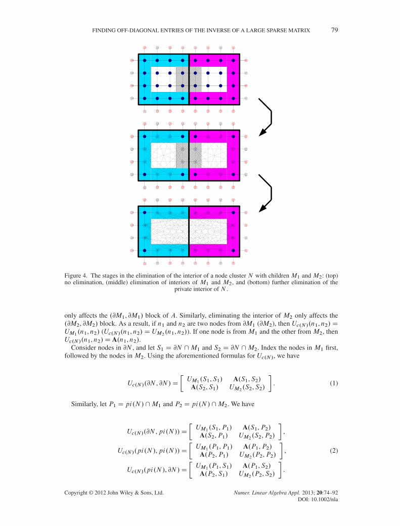
Figure 4 shows the steps involved in the elimination of the interior of a nonleaf node clusterN with children M1 and M2. The shaded region is @N , whereas the diagonal-textured region ispi.N /. The top mesh shows the mesh before any elimination of Int.N / has occurred. The middlemesh shows the elimination of Int.M1/ and Int.M2/. The final mesh shows the middle mesh afterpi.N / has been removed. These steps form the basic idea of the upwards pass algorithm.
Algorithm 1 describes the upwards pass algorithm in full detail. Let A be the original sparsematrix before any nodes have been removed. Consider a node cluster N with children M1 and M2.The goal of the upwards pass is to compute UN .@N , @N/ which is the reduced matrix A after theinterior of node cluster N has been removed. The idea is to eliminate the interior of node cluster Nby eliminating the interior of its children M1 and M2.
The algorithm starts with computing UM1 and UM2 by a recursive call to the upwards pass.It then computes Uc.N/, the reduced matrix A after the interiors of M1 and M2 have beenremoved. (Here, c.N / refers to the children of N .) Note that eliminating the interior of M1
Copyright © 2012 John Wiley & Sons, Ltd. Numer. Linear Algebra Appl. 2013; 20:74–92DOI: 10.1002/nla
FINDING OFF-DIAGONAL ENTRIES OF THE INVERSE OF A LARGE SPARSE MATRIX 79
Figure 4. The stages in the elimination of the interior of a node cluster N with children M1 and M2: (top)no elimination, (middle) elimination of interiors of M1 and M2, and (bottom) further elimination of the
private interior of N .
only affects the .@M1, @M1/ block of A. Similarly, eliminating the interior of M2 only affects the.@M2, @M2/ block. As a result, if n1 and n2 are two nodes from @M1 (@M2), then Uc.N/.n1,n2/DUM1.n1,n2/ (Uc.N/.n1,n2/ D UM2.n1,n2/). If one node is from M1 and the other from M2, thenUc.N/.n1,n2/D A.n1,n2/.
Consider nodes in @N , and let S1 D @N \M1 and S2 D @N \M2. Index the nodes in M1 first,followed by the nodes in M2. Using the aforementioned formulas for Uc.N/, we have
Uc.N/.@N , @N/D
�UM1.S1,S1/ A.S1,S2/
A.S2,S1/ UM2.S2,S2/
�. (1)
Similarly, let P1 D pi.N /\M1 and P2 D pi.N /\M2. We have
Uc.N/.@N ,pi.N //D
�UM1.S1,P1/ A.S1,P2/
A.S2,P1/ UM2.S2,P2/
�,
Uc.N/.pi.N /,pi.N //D
�UM1.P1,P1/ A.P1,P2/
A.P2,P1/ UM2.P2,P2/
�,
Uc.N/.pi.N /, @N/D
�UM1.P1,S1/ A.P1,S2/
A.P2,S1/ UM2.P2,S2/
�.
(2)
Copyright © 2012 John Wiley & Sons, Ltd. Numer. Linear Algebra Appl. 2013; 20:74–92DOI: 10.1002/nla

80 S. EASTWOOD AND J. W. L. WAN
Finally, we compute UN .@N , @N/ by eliminating the pi.N / nodes from the computational mesh,leaving us with the Schur complement:
UN .@N , @N/D Uc.N/.@N , @N/
�Uc.N/.@N ,pi.N //Uc.N/.pi.N /,pi.N //�1Uc.N/.pi.N /, @N/.
In the case where N is the root cluster, @N D ;, so UN .@N , @N/ stores an empty .0� 0/ matrix.
2.2. The downwards pass
After the upwards pass has been terminated, we will have computed UN .@N , @N/ for every nodecluster N .
Suppose that we are inverting A by performing simple forward reduction on the augmented matrix�A I
�. Let the arbitrary node n occur last in the ordering. After pivoting from all of the previ-
ous nodes, the bottom row becomes�0 : : : 0 u j � : : : � 1
�. u denotes the .n,n/
entry that remains after all nodes, other than n, have been eliminated, whereas each � denotes anunknown fill-in. Thus, A�1.n,n/D 1
u. Similarly, if node cluster N occurs last in the ordering, then
A�1.N ,N/ D U�1, where U is the .N ,N/ block of the reduced A after all nodes outside of Nhave been removed.
The overall aim of the downwards pass is to calculate A�1.N ,N/ for every leaf node cluster N .As described earlier, it is equivalent to finding the .N ,N/ block of the reduced matrix A obtainedfrom eliminating all nodes outside of N . We first define the following.
Definition 6Given a node cluster N , the ‘complement’ of N , denoted by N , is the set of all mesh nodes outsideof N .
Definition 7Given a node cluster N , the ‘adjacent’ of N , denoted by %N D @N , is the boundary of thecomplement of N .
Definition 8Given a node cluster N , the ‘exterior’ of N , denoted by Ext.N / D Int.N /, is the interior of thecomplement of N .
Similar to the upwards pass, we employ a divide-and-conquer method for eliminating the exteriornodes in the case of nonroot clusters. Consider a node cluster N with parent cluster P and sibling
Copyright © 2012 John Wiley & Sons, Ltd. Numer. Linear Algebra Appl. 2013; 20:74–92DOI: 10.1002/nla

FINDING OFF-DIAGONAL ENTRIES OF THE INVERSE OF A LARGE SPARSE MATRIX 81
cluster S . To eliminate the exterior of N , we first eliminate the exterior of P and the interior of S(note that N D P t S ). We will call the set of remaining nodes as the private exterior of N .
Definition 9Given a nonroot node cluster N with parent cluster P and sibling cluster S , the ‘private exterior’ ofN , denoted by pe.N /, is defined by pe.N /DExt.N /� .Ext.P /[ Int.S//.
Figure 5 depicts the adjacent and private exterior set for a node cluster N with parent cluster Pand sibling cluster S . The dark/red area is the adjacent set %N \ P of N, and the light/grey area isthe private exterior set pe.N / of N .
The notion of the exterior and private exterior node sets were not part of the notation used in [3].These definitions are introduced in this paper to simplify the discussion.
Algorithm 2 describes the downwards pass algorithm in full detail. The goal of the downwardspass is to compute UN .%N , %N/, the reduced matrix A after the exterior of N has been removed.The idea is to eliminate the exterior of N by eliminating the exterior of its parent P and the interiorof its sibling S .
The algorithm starts with calling DownwardsPass(Root), where Root denotes the root node clus-ter. After the computation of UN (which is just an empty matrix for Root), it makes a recursive callto compute UM1 and UM2 for its children M1 and M2.
At a general recursive step for a node cluster N , UP has already been computed for its parentcluster P . Also, US can be obtained from the upwards pass for its sibling cluster S . The algorithmthen computes Uf .N/, the result of eliminating both the exterior of the parent, and the interior ofthe sibling. (Here, f .N / refers to the ‘family’ of N .) Note that eliminating the exterior of P willonly affect the .%P , %P / block of A. Similarly, eliminating the interior of S will only affect the.@S , @S/ block. Thus, if n1 and n2 are two nodes from %P (@S ), then Uf .N/.n1,n2/D UP .n1,n2/(Uf .N/.n1,n2/ D US .n1,n2/). Otherwise, Uf .N/.n1,n2/ D A.n1,n2/. This is similar to thecomputation of Uc.N/ in the upwards pass.
Let X1 D %N \P , X2 D %N \S , Y1 D pe.N /\P , and Y2 D pe.N /\S . Also, index the nodesin P first, followed by the nodes in S . Using the aforementioned formulas for Uf .N/, we have
Uf .N/.%N , %N/D
�UP .X1,X1/ A.X1,X2/A.X2,X1/ US .X2,X2/
�,
Uf .N/.%N ,pe.N //D
�UP .X1,Y1/ A.X1,Y2/A.X2,Y1/ US .X2,Y2/
�,
Uf .N/.pe.N /,pe.N //D
�UP .Y1,Y1/ A.Y1,Y2/A.Y2,Y1/ US .Y2,Y2/
�,
Uf .N/.pe.N /, %N/D
�UP .Y1,X1/ A.Y1,X2/A.Y2,X1/ US .Y2,X2/
�.
(3)
Figure 5. An example showing the adjacent (dark) and private exterior (light) of a nonroot node cluster N .
Copyright © 2012 John Wiley & Sons, Ltd. Numer. Linear Algebra Appl. 2013; 20:74–92DOI: 10.1002/nla

82 S. EASTWOOD AND J. W. L. WAN
Then, we can compute UN .%N , %N/ by eliminating the pe.N / nodes from the computationalmesh, leaving us with the Schur complement:
UN .%N , %N/D Uf .N/.%N , %N/
�Uf .N/.%N ,pe.N //Uf .N/.pe.N /,pe.N //�1Uf .N/.pe.N /, %N/.
At the leaf node cluster, we finally eliminate the adjacent node set %N and invert the remaining.N ,N/ block.
3. THE ADVANCED FIND ALGORITHM
This section will describe the extensions to the FIND algorithm that will be made to compute theoff-diagonal entries of the inverse of A.
As in the previous section, suppose that we are inverting A by performing simple forward reduc-tion on the augmented matrix
�A I
�. Let the nodes n1 and n2 be the second-to-last and the
last nodes in the ordering, respectively. After pivoting from all nodes other than n1 and n2, the
bottom two rows of the augmented matrix become
�0 : : : 0
0 : : : 0U
� : : : � 1 0
� : : : � 0 1
�.
U denotes the fn1,n2g � fn1,n2g block that remains after all nodes other than n1 and n2 havebeen removed, whereas each � denotes an unknown fill-in. Multiplying the bottom two rows
by U�1 gives
�0 : : : 0 1 0
0 : : : 0 0 1
� : : : �� : : : �
U�1�
. The bottom two rows are not
affected by any of the subsequent row operations during back substitution, so we can concludethat A�1.n1,n2/D U�1.1, 2/ and A�1.n2,n1/D U�1.2, 1/. Similarly, if node clusters N1 and N2occur last in the ordering, then A�1.N1,N2/ D U�1.N1,N2/ and A�1.N2,N1/ D U�1.N2,N1/,where U denotes the .N1 tN2/ � .N1 tN2/ block that remains after all nodes that are outside ofN1 tN2 have been removed.
To summarize, FIND algorithm (downwards pass) computes the diagonal entries, A�1.n,n/, byeliminating the exterior of each node cluster. The main idea of our proposed method (‘advanced
Copyright © 2012 John Wiley & Sons, Ltd. Numer. Linear Algebra Appl. 2013; 20:74–92DOI: 10.1002/nla
FINDING OFF-DIAGONAL ENTRIES OF THE INVERSE OF A LARGE SPARSE MATRIX 83
downwards pass’) for computing the off-diagonal entries, A�1.n1,n2/, is to eliminate the exteriorof what we call the ‘node cluster pairs’.
3.1. Node cluster pairs
In this section, we define the notion of ‘node cluster pairs’, which is the key for computingoff-diagonal entries of the inverse. In addition, we extend the concepts of the node cluster tree,complement, adjacency, (private) interior, and (private) exterior for node cluster pairs.
Definition 10A ‘node cluster pair’ is an unordered pair of distinct node clusters that both exist on the same levelin the node cluster tree.
We now define the different types of node cluster pairs.
Definition 11A node cluster pair is called a ‘twin pair’ if the node clusters are siblings of each other. A nodecluster pair is called a ‘leaf pair’ if the node clusters exist at the leaf level of the node cluster tree.
We note that there is no ambiguity in the definition of the leaf pair because we specified thatthe node cluster tree will be perfectly balanced with all leaf clusters on the same level. Also, it ispossible for a node cluster pair to be both a twin pair and a leaf pair.
To accommodate the computation involving node cluster pairs, we need to extend the structure ofthe node cluster tree. The motivation behind these extensions will become clear when we describethe recursive algorithms that makeup the advanced downwards pass. The changes are as follows:
� Any nonleaf node cluster N with children M1 and M2 will receive a twin pair as an additionalchild. This twin pair will consist of the children of N , that is fM1,M2g, and is called the ‘twinchild’ of N .� Every nonleaf node cluster pair fN1,N2g has four children:
- child11.fN1,N2g/D fchild1.N1/, child1.N2/g,- child12.fN1,N2g/D fchild1.N1/, child2.N2/g,- child21.fN1,N2g/D fchild2.N1/, child1.N2/g,- child22.fN1,N2g/D fchild2.N1/, child2.N2/g.
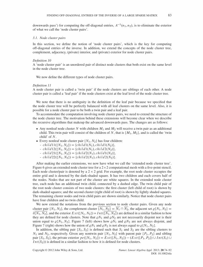
After making the earlier extensions, we now have what we call the ‘extended node cluster tree’.Figure 6 gives an extended node cluster tree for a 2�2 computational mesh with a five-point stencil.Each node cluster/pair is denoted by a 2 � 2 grid. For example, the root node cluster occupies theentire grid and is denoted by the dark-shaded square. It has two children and each covers half ofthe nodes. Nodes that are not part of the cluster are white squares. In the extended node clustertree, each node has an additional twin child, connected by a dashed edge. The twin child pair ofthe root node cluster consists of two node clusters: the first cluster (left child of root) is shown bydark-shaded squares; and the second cluster (right child of root) is shown by lightly shaded squares.The remaining cluster nodes and twin child pairs are shown similarly. Notice that node cluster pairshave four children and no twin child.
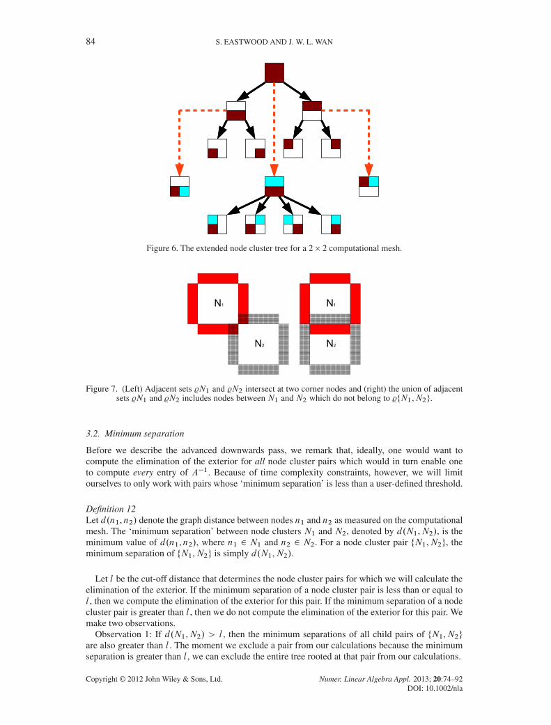
We now extend the notations from the previous section to node cluster pairs. Given any nodecluster pair fN1,N2g, the complement cluster fN1,N2g D N1 \N2, the adjacent set %fN1,N2g D@fN1,N2g, and the exteriorExt.fN1,N2g/ = Int.fN1,N2g/ are defined in a similar fashion to howthey are defined for node clusters. Note that %N1 and %N2 are not necessarily disjoint nor is theirunion equal to %fN1,N2g. Figure 7 (left) shows how %N1 and %N2 are not always disjoint, andFigure 7 (right) shows how the union of %N1 and %N2 is not always equal to %fN1,N2g.
In addition, the sibling pair fS1,S2g is defined such that S1 and S2 are the sibling clusters toN1 and N2, respectively. Given any nontwin pair fN1,N2g with parent pair fP1,P2g and siblingpair fS1,S2g, the private exterior pe.fN1, N2g/D Ext.fN1,N2g/� .Ext.fP1,P2g/[ Int.S1/[Int.S2// is defined in a similar fashion to how it is defined for node clusters.
Copyright © 2012 John Wiley & Sons, Ltd. Numer. Linear Algebra Appl. 2013; 20:74–92DOI: 10.1002/nla
84 S. EASTWOOD AND J. W. L. WAN
Figure 6. The extended node cluster tree for a 2� 2 computational mesh.
Figure 7. (Left) Adjacent sets %N1 and %N2 intersect at two corner nodes and (right) the union of adjacentsets %N1 and %N2 includes nodes between N1 and N2 which do not belong to %fN1,N2g.
3.2. Minimum separation
Before we describe the advanced downwards pass, we remark that, ideally, one would want tocompute the elimination of the exterior for all node cluster pairs which would in turn enable oneto compute every entry of A�1. Because of time complexity constraints, however, we will limitourselves to only work with pairs whose ‘minimum separation’ is less than a user-defined threshold.
Definition 12Let d.n1,n2/ denote the graph distance between nodes n1 and n2 as measured on the computationalmesh. The ‘minimum separation’ between node clusters N1 and N2, denoted by d.N1,N2/, is theminimum value of d.n1,n2/, where n1 2 N1 and n2 2 N2. For a node cluster pair fN1,N2g, theminimum separation of fN1,N2g is simply d.N1,N2/.
Let l be the cut-off distance that determines the node cluster pairs for which we will calculate theelimination of the exterior. If the minimum separation of a node cluster pair is less than or equal tol , then we compute the elimination of the exterior for this pair. If the minimum separation of a nodecluster pair is greater than l , then we do not compute the elimination of the exterior for this pair. Wemake two observations.
Observation 1: If d.N1,N2/ > l , then the minimum separations of all child pairs of fN1,N2gare also greater than l . The moment we exclude a pair from our calculations because the minimumseparation is greater than l , we can exclude the entire tree rooted at that pair from our calculations.
Copyright © 2012 John Wiley & Sons, Ltd. Numer. Linear Algebra Appl. 2013; 20:74–92DOI: 10.1002/nla
FINDING OFF-DIAGONAL ENTRIES OF THE INVERSE OF A LARGE SPARSE MATRIX 85
Observation 2: If d.N1,N2/ 6 l , then there exists at least one child pair of fN1,N2g thathas a minimum separation less than or equal to l . When we include a pair in our calculationsbecause the minimum separation is less than or equal to l , we can move on to at least one of thechild pairs.
The aforementioned two observations imply that if we restrict the extended node cluster treeas to exclude pairs whose minimum separation is greater than l , the resultant tree is connectedbecause of the first observation. Also, there are no ‘dead ends’ in the sense that there alwaysexists a nonempty child pair before we reach the leaf node or leaf-pair level because of thesecond observation.
3.3. Advanced downwards pass
We will now describe the advanced downwards pass, which will replace the downwards pass. Theessence of the advanced downwards pass is not much different from the downward pass. It com-putes the elimination of the exterior of the node clusters. However, in addition, it also computes theelimination of the exterior of node cluster pairs. This is the main difference from the downwardspass that enables us to compute off-diagonal entries of the inverse.
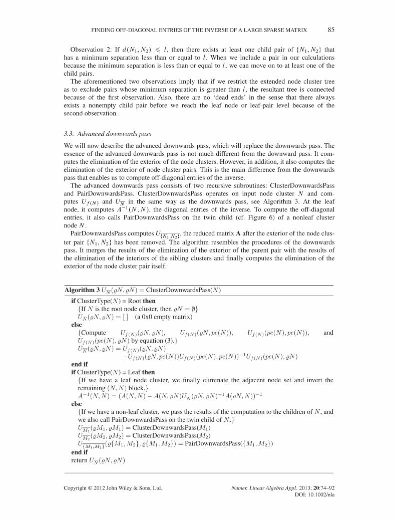
The advanced downwards pass consists of two recursive subroutines: ClusterDownwardsPassand PairDownwardsPass. ClusterDownwardsPass operates on input node cluster N and com-putes Uf .N/ and UN in the same way as the downwards pass, see Algorithm 3. At the leafnode, it computes A�1.N ,N/, the diagonal entries of the inverse. To compute the off-diagonalentries, it also calls PairDownwardsPass on the twin child (cf. Figure 6) of a nonleaf clusternode N .
PairDownwardsPass computes UfN1,N2g, the reduced matrix A after the exterior of the node clus-
ter pair fN1,N2g has been removed. The algorithm resembles the procedures of the downwardspass. It merges the results of the elimination of the exterior of the parent pair with the results ofthe elimination of the interiors of the sibling clusters and finally computes the elimination of theexterior of the node cluster pair itself.
Copyright © 2012 John Wiley & Sons, Ltd. Numer. Linear Algebra Appl. 2013; 20:74–92DOI: 10.1002/nla
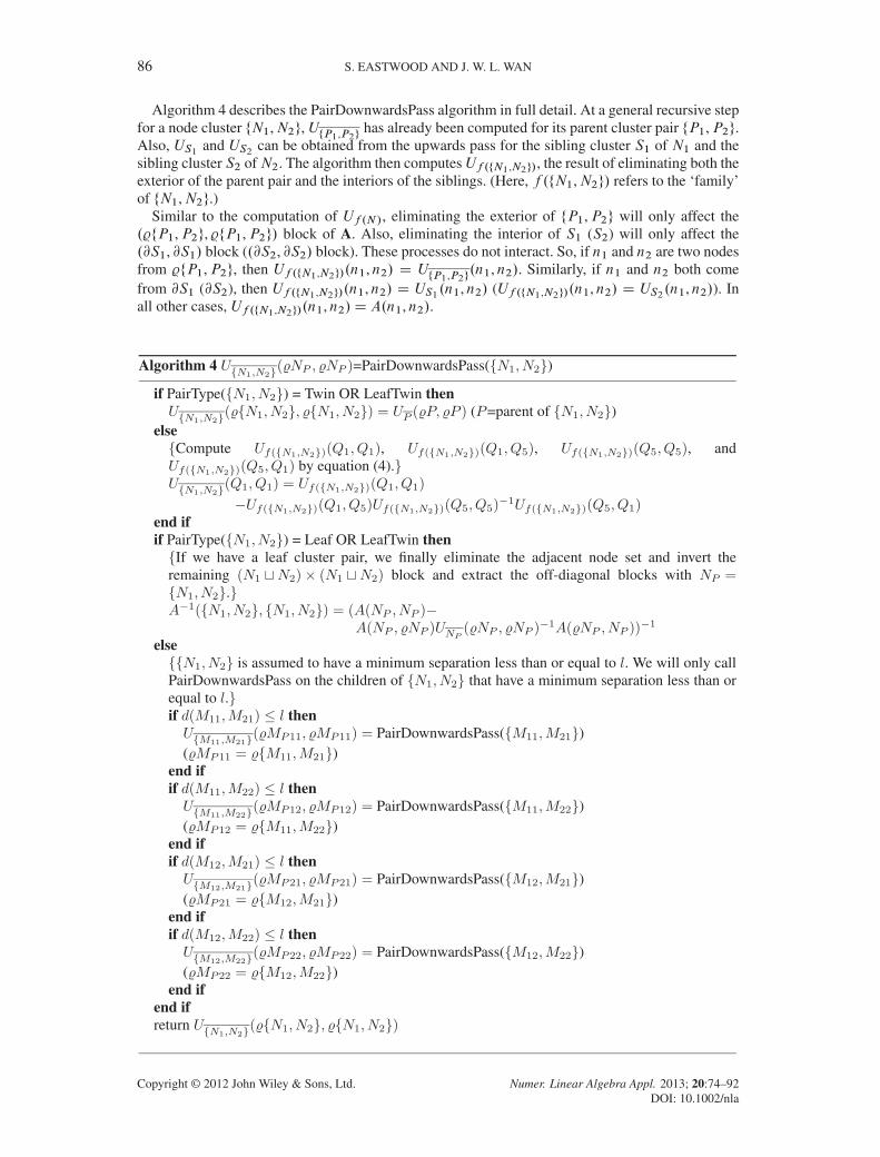
86 S. EASTWOOD AND J. W. L. WAN
Algorithm 4 describes the PairDownwardsPass algorithm in full detail. At a general recursive stepfor a node cluster fN1,N2g, UfP1,P2g
has already been computed for its parent cluster pair fP1,P2g.Also, US1 and US2 can be obtained from the upwards pass for the sibling cluster S1 of N1 and thesibling cluster S2 ofN2. The algorithm then computes Uf .fN1,N2g/, the result of eliminating both theexterior of the parent pair and the interiors of the siblings. (Here, f .fN1,N2g/ refers to the ‘family’of fN1,N2g.)
Similar to the computation of Uf .N/, eliminating the exterior of fP1,P2g will only affect the.%fP1,P2g, %fP1,P2g/ block of A. Also, eliminating the interior of S1 (S2) will only affect the.@S1, @S1/ block (.@S2, @S2/ block). These processes do not interact. So, if n1 and n2 are two nodesfrom %fP1,P2g, then Uf .fN1,N2g/.n1,n2/ D UfP1,P2g
.n1,n2/. Similarly, if n1 and n2 both comefrom @S1 (@S2), then Uf .fN1,N2g/.n1,n2/ D US1.n1,n2/ (Uf .fN1,N2g/.n1,n2/ D US2.n1,n2/). Inall other cases, Uf .fN1,N2g/.n1,n2/D A.n1,n2/.
Copyright © 2012 John Wiley & Sons, Ltd. Numer. Linear Algebra Appl. 2013; 20:74–92DOI: 10.1002/nla
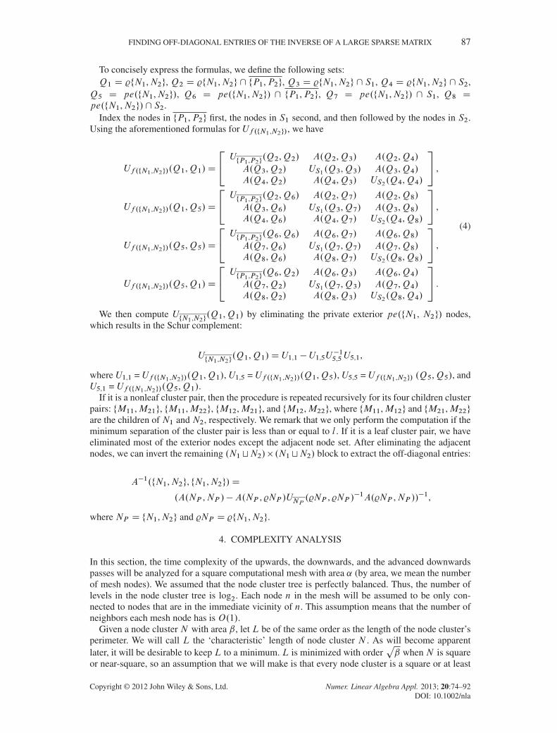
FINDING OFF-DIAGONAL ENTRIES OF THE INVERSE OF A LARGE SPARSE MATRIX 87
To concisely express the formulas, we define the following sets:Q1 D %fN1,N2g, Q2 D %fN1,N2g \ fP1,P2g, Q3 D %fN1,N2g \ S1, Q4 D %fN1,N2g \ S2,
Q5 D pe.fN1,N2g/, Q6 D pe.fN1,N2g/ \ fP1,P2g, Q7 D pe.fN1,N2g/ \ S1, Q8 Dpe.fN1,N2g/\ S2.
Index the nodes in fP1,P2g first, the nodes in S1 second, and then followed by the nodes in S2.Using the aforementioned formulas for Uf .fN1,N2g/, we have
Uf .fN1,N2g/.Q1,Q1/D
24 UfP1,P2g
.Q2,Q2/ A.Q2,Q3/ A.Q2,Q4/
A.Q3,Q2/ US1.Q3,Q3/ A.Q3,Q4/
A.Q4,Q2/ A.Q4,Q3/ US2.Q4,Q4/
35 ,
Uf .fN1,N2g/.Q1,Q5/D
24 UfP1,P2g
.Q2,Q6/ A.Q2,Q7/ A.Q2,Q8/
A.Q3,Q6/ US1.Q3,Q7/ A.Q3,Q8/
A.Q4,Q6/ A.Q4,Q7/ US2.Q4,Q8/
35 ,
Uf .fN1,N2g/.Q5,Q5/D
24 UfP1,P2g
.Q6,Q6/ A.Q6,Q7/ A.Q6,Q8/
A.Q7,Q6/ US1.Q7,Q7/ A.Q7,Q8/
A.Q8,Q6/ A.Q8,Q7/ US2.Q8,Q8/
35 ,
Uf .fN1,N2g/.Q5,Q1/D
24 UfP1,P2g
.Q6,Q2/ A.Q6,Q3/ A.Q6,Q4/
A.Q7,Q2/ US1.Q7,Q3/ A.Q7,Q4/
A.Q8,Q2/ A.Q8,Q3/ US2.Q8,Q4/
35 .
(4)
We then compute UfN1,N2g.Q1,Q1/ by eliminating the private exterior pe.fN1, N2g/ nodes,
which results in the Schur complement:
UfN1,N2g.Q1,Q1/D U1,1 �U1,5U
�15,5U5,1,
where U1,1 = Uf .fN1,N2g/.Q1,Q1/, U1,5 = Uf .fN1,N2g/.Q1,Q5/, U5,5 = Uf .fN1,N2g/ .Q5,Q5/, andU5,1 = Uf .fN1,N2g/.Q5,Q1/.
If it is a nonleaf cluster pair, then the procedure is repeated recursively for its four children clusterpairs: fM11,M21g, fM11,M22g, fM12,M21g, and fM12,M22g, where fM11,M12g and fM21,M22gare the children of N1 and N2, respectively. We remark that we only perform the computation if theminimum separation of the cluster pair is less than or equal to l . If it is a leaf cluster pair, we haveeliminated most of the exterior nodes except the adjacent node set. After eliminating the adjacentnodes, we can invert the remaining .N1tN2/� .N1tN2/ block to extract the off-diagonal entries:
A�1.fN1,N2g, fN1,N2g/D
.A.NP ,NP /�A.NP , %NP /UNP .%NP , %NP /�1A.%NP ,NP //
�1,
where NP D fN1,N2g and %NP D %fN1,N2g.
4. COMPLEXITY ANALYSIS
In this section, the time complexity of the upwards, the downwards, and the advanced downwardspasses will be analyzed for a square computational mesh with area ˛ (by area, we mean the numberof mesh nodes). We assumed that the node cluster tree is perfectly balanced. Thus, the number oflevels in the node cluster tree is log2. Each node n in the mesh will be assumed to be only con-nected to nodes that are in the immediate vicinity of n. This assumption means that the number ofneighbors each mesh node has is O.1/.
Given a node cluster N with area ˇ, let L be of the same order as the length of the node cluster’sperimeter. We will call L the ‘characteristic’ length of node cluster N . As will become apparentlater, it will be desirable to keep L to a minimum. L is minimized with order
pˇ when N is square
or near-square, so an assumption that we will make is that every node cluster is a square or at least
Copyright © 2012 John Wiley & Sons, Ltd. Numer. Linear Algebra Appl. 2013; 20:74–92DOI: 10.1002/nla

88 S. EASTWOOD AND J. W. L. WAN
a near-square rectangle. Thus, nonleaf node clusters are divided into their child clusters by a cutparallel to their shorter dimension.
During the upwards, downwards, and the advanced downwards passes, we perform the following
computation at each node cluster/pair: Start with the block matrix
�X Y
Z W
�, whereX is ���, Y
is ���, Z is ���, andW is a ���. We then block reduce to obtain
�X Y
0 W �ZX�1Y
�. Effi-
ciently computing U DW �ZX�1Y will require ��2C 13�3C�2� multiplication flops, neglecting
lower-order terms.
� When we perform the upwards pass on nonleaf node clusters N , �D jpi.N /j, and � D j@N j.� When we perform the downwards pass on nonroot node clusters N , � D jpe.N /j, and� D j%N j.� When we perform the advanced downwards pass on a nontwin node cluster pair fN1,N2g,�D jpe.fN1,N2g/j, and � D j%fN1,N2gj.
In all these cases, � and � have order L. Therefore, the complexity of computing U DO.L3/DO.ˇ3=2/.
We now label the root level of the extended node cluster tree as Level 0 and the subsequent levelsas Level 1, 2, etc. At Level i , there are exactly 2i node clusters. Although there are approximately4i node cluster pairs at level i , we only need to consider the pairs whose minimum separation is lessthan or equal to l . The following will give an informal geometric argument to determine the orderof the number of pairs at level i whose minimum separation is less or equal to l .
Let N be any node cluster at level i . Denote the number of level i node clusters other than N ,whose minimum separation from N is less than or equal to l by k.N /. The number of level i pairswhose minimum separation is less than or equal to l is then given by 1
2
Pk.N /. If we simply find
the magnitude order of k.N /, we can multiply it by 2i to obtain the order of the number of level ipairs whose minimum separation is less than or equal to l .
We now derive the magnitude order of the number of level i pairs for the following two cases:Case 1: 06 i 6 log2
˛l2
In this case, the characteristic length L Dq
˛
2iof N satisfies L > l . L > l implies that the
number of level i node clusters whose minimum separation fromN is less than or equal to l isO.1/because there are onlyO.1/ node clusters aroundN because of a relatively large size. Figure 8 (left)shows an example when L> l . In this case, only eight neighboring node clusters are within l of N .Hence, the number of pairs at level i whose minimum separation is less than or equal to l is O.2i /.
Figure 8. Number of node clusters whose minimum separation from N 6 l for (left) large node clusters(L> l) and (right) small node clusters (L6 l).
Copyright © 2012 John Wiley & Sons, Ltd. Numer. Linear Algebra Appl. 2013; 20:74–92DOI: 10.1002/nla
FINDING OFF-DIAGONAL ENTRIES OF THE INVERSE OF A LARGE SPARSE MATRIX 89
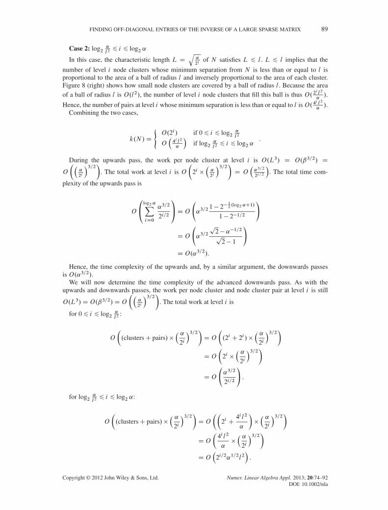
Case 2: log2˛l26 i 6 log2 ˛
In this case, the characteristic length L Dq
˛
2iof N satisfies L 6 l . L 6 l implies that the
number of level i node clusters whose minimum separation from N is less than or equal to l isproportional to the area of a ball of radius l and inversely proportional to the area of each cluster.Figure 8 (right) shows how small node clusters are covered by a ball of radius l . Because the areaof a ball of radius l is O.l2/, the number of level i node clusters that fill this ball is thus O.2
i l2
˛/.
Hence, the number of pairs at level i whose minimum separation is less than or equal to l isO.4i l2
˛/.
Combining the two cases,
k.N /D
(O.2i / if 06 i 6 log2
˛l2
O�4i l2
˛
�if log2
˛l26 i 6 log2 ˛
.
During the upwards pass, the work per node cluster at level i is O.L3/ D O.ˇ3=2/ D
O
��˛
2i
�3=2. The total work at level i is O
�2i �
�˛
2i
�3=2D O
�˛3=2
2i=2
�. The total time com-
plexity of the upwards pass is
O
0@log2 ˛XiD0
˛3=2
2i=2
1ADO
˛3=2
1� 2�12 .log2 ˛C1/
1� 2�1=2
!
DO
˛3=2p2� ˛�1=2p2� 1
!
DO.˛3=2/.
Hence, the time complexity of the upwards and, by a similar argument, the downwards passesis O.˛3=2/.
We will now determine the time complexity of the advanced downwards pass. As with theupwards and downwards passes, the work per node cluster and node cluster pair at level i is still
O.L3/DO.ˇ3=2/DO
��˛
2i
�3=2. The total work at level i is
for 06 i 6 log2˛l2
:
O
�.clustersC pairs/�
� ˛2i
�3=2DO
�.2i C 2i /�
� ˛2i
�3=2
DO
�2i �
� ˛2i
�3=2
DO
˛3=2
2i=2
!.
for log2˛l26 i 6 log2 ˛:
O
�.clustersC pairs/�
� ˛2i
�3=2DO
��2i C
4i l2
˛
�� ˛2i
�3=2
DO
�4i l2
˛�� ˛2i
�3=2
DO�2i=2˛1=2l2
�.
Copyright © 2012 John Wiley & Sons, Ltd. Numer. Linear Algebra Appl. 2013; 20:74–92DOI: 10.1002/nla

90 S. EASTWOOD AND J. W. L. WAN
The total time complexity of the advanced downwards pass is
O
0B@
log2˛
l2XiD0
˛3=2
2i=2C
log2 ˛XiDlog2
˛
l2
2i=2˛1=2l2
1CA
DO
˛3=2
1� 2� 12 .log2
˛
l2C1/
1� 2�1=2C 2
12 log2
˛
l2 ˛1=2l2212 .log2 l
2C1/ � 1
21=2 � 1
!
DO
˛3=2p2� ˛�
12 l
p2� 1
C ˛llp2� 1
p2� 1
!
DO.˛3=2C ˛l2/.
Hence, the time complexity of the advanced downwards pass isO.˛3=2C˛l2/. Note that if l D 0,which means that we are computing no off-diagonal entries, then the time complexity is O.˛3=2/which is the same as the upwards and downwards passes. If l D
p˛, which means that we are
computing all off-diagonal entries, then the time complexity is O.˛2/ which is the minimum timecomplexity required to compute every entry of the inverse.
The highest order for cut-off distance l that will still result in a time complexity of O.˛3=2/ forthe advanced downwards pass is l DO.˛1=4/. In other words, l must have, at most, the same orderas the square root of the computational mesh’s width if the time complexity is to remain atO.˛3=2/.
Given a cut-off distance of l , it is of interest to note that the number of entries of A�1 that willultimately be computed is of the same order as the number of leaf pairs whose minimum separationis less than or equal to l . The number of leaf pairs whose minimum separation is less than or equalto l is O.4
log2 ˛l2
˛/D O.˛
2l2
˛/D O.˛l2/ (Here, we used the case 2 result derived when computing
the number of level i pairs whose minimum separation is less than or equal to l). If we let the cut-offdistance l D ˛1=4C� where 0 6 � 6 1=4, then we will be computing O.˛3=2C2�/ entries of A�1.Because the computational time complexity in this case is alsoO.˛3=2C2�/, the computational timecomplexity per entry of A�1 calculated is O.1/. This concludes the result stated in the abstract.
5. NUMERICAL RESULTS
In this section, we will demonstrate that the computational complexity of the advanced FIND algo-rithm is O.˛3=2/, provided that the cut-off distance l is O.˛1=4/. The example scenario that wasused in measuring the flop counts is an L � L square computational mesh utilizing a five-pointstencil. The sparse matrix used was the five-point stencil approximation of the Laplacian operator.The node cluster tree depth is chosen to be deep enough so that all leaf node clusters have either 0or 1 nodes. More precisely, the node cluster tree depth used for an L � L computational mesh is2dlog2.L/e. The cut-off distance l used for an L�L computational mesh is l D b
pLc.
Figure 9 is a base 2 log-log plot of the multiplication flops used versus the grid size L. Theupper curve (interpolated from the points denoted by squares) shows the number of flops used inthe upwards pass and advanced downwards pass, that is, the advanced FIND algorithm. The lowercurve (interpolated from the points denoted by diamonds), included for reference, shows the numberof flops used in the upwards pass and downwards pass, that is, the original FIND algorithm. As weare trying to show that the computational complexity is O.˛3=2/ D O.L3/, the upper curve musttend towards having a slope of 3. The straight line included indicates a slope of 3. As can be seen,both the upper and the lower curves become increasingly parallel to the straight line.
Notice that the upper curve in Figure 9 has a number of apparent jumps: between grid sizes 8 and9; between grid sizes 15 and 16; between grid sizes 24 and 25; and between grid sizes 35 and 36.Recalling that the cut-off distance l D b
pLc, the jumps correspond exactly when l increases by 1.
Figure 10 is a base 2 log-log plot of run time versus the grid size. Again, the upper curve denotesthe advanced FIND algorithm and the lower curve denotes the original FIND algorithm. The straight
Copyright © 2012 John Wiley & Sons, Ltd. Numer. Linear Algebra Appl. 2013; 20:74–92DOI: 10.1002/nla

FINDING OFF-DIAGONAL ENTRIES OF THE INVERSE OF A LARGE SPARSE MATRIX 91
Figure 9. A base 2 log-log plot of flops versus grid size.
Figure 10. A base 2 log-log plot of CPU time versus grid size.
line included indicates a slope of 3. As can be seen, both the upper and the lower curves are (roughly)parallel to the straight line.
Both the upper and the lower curves in Figure 10 jump dramatically whenever the node clustertree depth, 2dlog2.L/e, increases. This behavior, which is evident in the curves for both the originalFIND algorithm and the advanced FIND algorithm, is caused primarily by a dramatic increase inthe amount of integer computations that accompany the increase in the node cluster tree size. Ateach ‘step’, the depth of the node cluster tree increases by 2, and because the node cluster tree is abinary tree, this means that the number of node clusters has increased by fourfold. The upper curvealso exhibits smaller jumps whenever the cut-off distance l D b
pLc increases. Despite this, both
curves still exhibit an overall slope of approximately 3.
6. CONCLUSION
We have extended the algorithm first described in [3] to now calculate off-diagonal entries of theinverse of a large sparse matrix corresponding to a square computational mesh. The applicationgiven in the introduction of finding the Green’s function for quantum nanodevices motivates thecentral idea that entries of the inverse that correspond to geometrically closer pairs of vertexes in thecomputational mesh are more important than entries of the inverse that correspond to more separatedpairs of vertexes. Diagonal entries, which correspond to connections of length 0, have the highestpriority. The extended algorithm computes all entries of the inverse that correspond to connectionsshorter than a given cut-off distance l . We proved that if l is of the order of O.˛1=4C�/, where ˛ isthe number of nodes in the square mesh and where 06 � 6 1=4 is arbitrary, then the computational
Copyright © 2012 John Wiley & Sons, Ltd. Numer. Linear Algebra Appl. 2013; 20:74–92DOI: 10.1002/nla

92 S. EASTWOOD AND J. W. L. WAN
time complexity is O.˛3=2C2�/ and the number of inverse entries computed is also O.˛3=2C2�/,resulting in a constant amount time per entry computed. For � D 0, we obtain O.˛3=2/ additionaloff-diagonal entries while not changing the time complexity of the FIND algorithm given by [3]which is O.˛3=2/.
REFERENCES
1. George A. Nested dissection of a regular finite element mesh. SIAM Journal on Numerical Analysis 1973;10(2):345–363.
2. George A, Liu, Joseph W H. Computer Solution of Large Sparse Positive Definite Systems. Englewood Cliffs: N.J.,Prentice-Hall, 1981.
3. Li S, Ahmed S, Klimeck G, Darve E. Computing entries of the inverse of a sparse matrix using the FIND algorithm.Journal of Computational Physics 2008; 227:9408–9427.
4. Erisman AM, Tinney WF. On computing certain elements of the inverse of a sparse matrix. Communications of theACM 1975; 18(3):177–179.
5. Darve E, et al. A hybrid method for the parallel computation of Green’s functions. Journal of Computational Physics2009; 228:5020–5039.
6. Lin L, Lu J, Ying L, Car R, E W. Fast algorithm for extracting the diagonal of the inverse matrix with application tothe electronic structure analysis of metallic systems. Communications in Mathematical Sciences 2009; 7(3):755–777.
7. Svizhenko A, Anantram MP, Govindan TR, Biegel B, Venugopal R. Two-dimensional quantum mechanical modelingof nanotransistors. Journal of Applied Physics 2002; 91(4):2343–2354.
8. Anantram MP, Svizhenko A. Multidimensional modeling of nanotransistors. IEEE transactions on Electron Devices2007; 54(9):2100–2115.
Copyright © 2012 John Wiley & Sons, Ltd. Numer. Linear Algebra Appl. 2013; 20:74–92DOI: 10.1002/nla

![Technical Datasheet - Veracious Inc · Inverse Characteristics Curve [Over Current IDMT]: Very Inverse Long Inverse Standard Inverse Extremely Inverse α C 0.02 1 2 1 0.14 13.5 80](https://static.fdocuments.in/doc/165x107/60dab49f5dabad678957ab65/technical-datasheet-veracious-inc-inverse-characteristics-curve-over-current.jpg)


![Non-Unit Bidiagonal Matrices for Factorization of ... · Higham [2] that entries of the inverse Vandermonde lower triangular components should be distinct and in ascending order.](https://static.fdocuments.in/doc/165x107/5ea7553b3edb4836c462a4ee/non-unit-bidiagonal-matrices-for-factorization-of-higham-2-that-entries-of.jpg)


