Finding, Minimizing, and Counting Weighted Subgraphs∗†

Virginia Vassilevska Williams‡ Ryan Williams§

Abstract

For a pattern graph H on k nodes, we consider the problems of finding and counting the number of (not necessarilyinduced) copies of H in a given large graph G on n nodes, as well as finding minimum weight copies in both node-weighted and edge-weighted graphs. Our results include:

• The number of copies of an H with an independent set of size s can be computed exactly in O∗(2snk−s+3)time. A minimum weight copy of such an H (with arbitrary real weights on nodes and edges) can be found inO(4s+o(s)nk−s+3) time. (The O∗ notation omits poly(k) factors.) These algorithms rely on fast algorithmsfor computing the permanent of a k × n matrix, over rings and semirings.

• The number of copies of any H having minimum (or maximum) node-weight (with arbitrary real weights onnodes) can be found in O(nωk/3 + n2k/3+o(1)) time, where ω < 2.4 is the matrix multiplication exponentand k is divisible by 3. Similar results hold for other values of k. Also, the number of copies having exactly aprescribed weight can be found within this time. These algorithms extend the technique of Czumaj and Lingas(SODA 2007) and give a new (algorithmic) application of multiparty communication complexity.

• Finding an edge-weighted triangle of weight exactly 0 in general graphs requires Ω(n3−ε) time for all ε > 0,unless the 3SUM problem on N numbers can be solved in O(N2−ε) time. This suggests that the edge-weightedproblem is much harder than its node-weighted version.

1 Introduction

We consider the problems of finding and counting the copies of a fixed k node graph H in a given n node graph G(such copies are called H-subgraphs). We also study the case of finding and counting maximum weight copies whenG has arbitrary real weights on its vertices or edges.

Subgraphs With Large Independent Sets In the unweighted case, the best known algorithm for counting H-subgraphs uses Coppersmith-Winograd matrix multiplication [16] and runs in Ω(nωk/3) ≥ Ω(n0.791k) time and nΘ(k)

space, where ω < 2.376 is the smallest exponent for which n×n matrix multiplication is in nω+o(1) time. We presentalgorithms that do not rely on fast matrix multiplication, yet still beat the above in both runtime and space usage, forH with a large independent set. In particular, if H has an independent set of size s, we can count the number of copiesofH in an n-node graph in polynomial space andO(4s+o(s)nk−sn3) orO(s! ·nk−sn2) time, or inO(2snk−sn3) timeand space. Our polynomial space algorithms can also be used to find minimum weight H-subgraphs in a graph witharbitrary real edge weights. These improvements are obtained via new algorithms for computing the permanent of arectangular matrix over a semiring. Our algorithms are simple and the runtime analysis does not hide huge constants.

Our results on counting and finding maximum subgraphs are interesting for both practical and theoretical reasons.On the practical side, pattern subgraph counting and detection are used in diverse areas, including the analysis of socialnetworks [8, 45, 42], computational biology, and network security [14, 25, 43]. In molecular biology, biomolecular∗The first author is currently supported by NSF Grant 0937060 to the Computing Research Association for the CIFellows Project. The second

author is currently supported by the Josef Raviv Memorial Fellowship. This material is based in part on work done while the authors were membersof the Institute for Advanced Study in Princeton. The authors were supported in part by NSF grant CCF-0832797 at Princeton University/IAS andPrinceton University sub-contract to IAS No.00001583. Any opinions, findings and conclusions or recommendations expressed are those of theauthors and do not necessarily reflect the views of the National Science Foundation.†A preliminary version of this paper appeared in the proceedings of STOC 2009.‡University of Calfornia, Berkeley, Berkeley, CA 94720 USA Email: virgi@cs.berkeley.edu.§IBM Almaden Research Center, San Jose, CA 95120 USA. Email: ryanwill@us.ibm.com.

1

networks are compared by identifying so-called network motifs [33] – connectivity patterns that occur much more fre-quently than expected in a random graph. Similar techniques are used to detect abnormal patterns in social networks(potential spammers, bots) and undesirable usage patterns in a computer network. Because of the extensive computa-tional overhead of previous exact counting techniques, approximate counting based on the color-coding technique [4]is typically used for pattern graphs on at least 4 nodes (e.g. [1]). Unfortunately, even for approximately counting trees,the current methods are not efficient for patterns with more than 9 nodes. Because some of the pattern graphs havelarge independent sets, we suspect our methods will be useful in the above settings: for instance, trees with manyleaves will be counted fairly quickly.

On the theoretical side, our algorithms are interesting because the problem of counting k-subgraphs (even k-paths)is #W [1]-complete (whereas approximately counting k-paths is not, cf. [2, 22, 6]). Hence if one could obtain aO(nα(k)) time algorithm for counting for a small enough function α, the Exponential Time Hypothesis would befalse, and many NP problems would have subexponential algorithms. Alon and Gutner [2] have proven in a formalsense that the color-coding method cannot hope to do better than O(nk/2) for counting paths exactly. As we obtainO(f(k)nk/2+c) algorithms, our results may be optimal in some sense (although they do not use color-coding).

Node-Weighted Subgraphs Via Matrix Products In the second part of the paper, we give algorithms that applyfast matrix multiplication to find and count weighted H-subgraphs for general H . We consider three variants of theproblem: finding and counting H-subgraphs of maximum weight, weight at least K, and weight exactly K (for anygiven weight K). Due to its relation to the all pairs shortest paths problem (APSP), the maximum weight version hasreceived much attention (e.g. [46, 47, 19]). The authors have recently shown that APSP and the related maximumweight triangle problem in edge-weighted graphs are equivalent under subcubic reductions [48] so that maximumweight triangle has a truly subcubic algorithm if and only if all pairs shortest paths does.

The current best algorithm for finding a maximum weight H-subgraph in a node-weighted graph is by Czumaj andLingas [19] and runs inO(nωk/3+ε) time for all ε > 0 (when k is divisible by 3; other cases are similar). We show howto extend their approach to counting maximum weight H-subgraphs in the same time. Moreover, we show that theproblem of counting the number of H-subgraphs of node weight at least K and even exactly K can also be done in thesame time. The previous best algorithm for either of these problems is based on the dominance product method [46]and has a running time of O(n

(3+ω)2

k3 ) (for k divisible by 3). Our algorithms rely on a new O(nω + n22O(

√logn))

algorithm for counting the number of triangles of weight K in a node-weighted graph. In fact, we give two verydifferent algorithms for exact node-weighted triangles: one based on the Czumaj-Lingas approach, and one based ona counterintuitive 3-party communication protocol for the Exactly-W problem.

Hardness Results for Edge-Weighted Subgraphs Finally, we provide theoretical evidence that finding edge weightedH-subgraphs faster than in O(nk) time will be difficult, for general H in arbitrary weighted graphs. We focus on theproblem of finding triangles of weight exactly K in an edge-weighted graph. Just as the maximum weight triangleproblem in edge-weighted graphs, this exact weight triangle problem is not known to have a truly subcubic algorithm,even though there is an extremely simple cubic time algorithm for it. In an attempt to explain this, we relate theexact-weight triangle problem to the 3SUM problem: given a list of n integers, determine whether there are three ofthem that sum up to 0. We first prove that unless 3SUM has a truly subquadratic algorithm, a triangle of weight sumK in an edge weighted graph cannot be found in O(n2.5−ε) time for any ε > 0. 3SUM is widely believed to requireessentially quadratic time (cf. [7] for a slight improvement), so our result suggests that the exact triangle problem foredge-weighted graphs is harder than that for node-weighted graphs. Patrascu [38] has recently proven a tight resultrelating 3SUM to a related problem, Convolution–3SUM. We show that using this relationship, our conditional lowerbound for exact weighted triangles can be improved optimally, i.e. unless 3SUM has truly subquadratic algorithms,finding a triangle of weight 0 in an edge-weighted graph requires essentally cubic time(!). We also show that sub-cubic algorithms for edge weighted triangle imply faster-than-2n algorithms for multivariate quadratic equations, animportant NP-complete problem in cryptography.

Prior Work Besides the references we have already mentioned, the theoretical problems of subgraph finding andcounting are discussed in many works, for example [27, 36, 15, 30, 44]. Alon, Yuster and Zwick [5] showed thatfor all k ≤ 7 the number of k-cycles in an unweighted graph can be computed in O(nω) time using fast matrixmultiplication. Unfortunately their approach does not seem to generalize for k > 7. Bjorklund et al. [10] have

2

recently found an interesting algorithm for counting k-paths that runs in(nk/2

)poly(n) time. For sufficiently large k,

their algorithm is faster than ours. However, their algorithm only works for k-paths and uses Ω((nk/2

)) space. For the

special case where H is a bipartite graph, our algorithm uses 2k+o(k)nk/2+3 time and poly(n, k) space.

Preliminaries For a node u in a graph (V,E), N(u) = v ∈ V | (u, v) ∈ E. For an integer n, let [n] =1, 2, . . . , n.

A graph homomorphism f from a graph G = (V,E) to a graph H = (VH , EH) is a mapping f : V → VH so thatif (u, v) ∈ E, then (f(u), f(v)) ∈ EH . A graph isomorphism f from a graph G = (V,E) to a graph H = (VH , EH)is a bijective map from G to H such that both f and f−1 are homomorphisms. An automorphism is an isomorphismbetween a graph G and itself. A k-path in a graph is a sequence of k distinct vertices, every two consecutive ones ofwhich are connected by an edge. A DAG is a directed graph with no cycles.

As usual, we define ω as the infimum of all real numbers such that n× n multiplication can be solved in nω+o(1)

arithmetic operations. The current best upper bound on ω is 2.376 [16].We say an algorithm on n × n matrices with entries in [−M,M ] (or n-node graphs with edge weights from

[−M,M ]) is truly subcubic if it runs in O(n3−δ · poly(logM)) time for some δ > 0.

2 Algorithms Without Matrix Multiplication

We begin by reducing the problems of counting and minimizing subgraphs to computing permanents of rectangularmatrices. We assume that all given graphs are undirected, but it is not hard to modify the proofs for directed graphs.

Theorem 2.1 Suppose the permanent of an s × n matrix can be computed in T (n, s) time and S(n, s) space. LetH = h1, . . . , hk be a graph on k nodes with an independent set of size s. Let G = (V,E) be a graph on n nodesand w : E → R be a weight function. Let C be the set of all (not necessarily induced) copies of H in G. Then thequantity ∑

Q∈C

∏e∈E(Q)

w(e)

can be determined in O((nks+ T (n, s)) · (k − s)!(nk−s)) time and O(ns+ S(n, s)) space.

Note that when w(e) = 1 for all e ∈ E, the quantity in the theorem is just the number of (not necessarily induced)copies of H in G.

Proof: Let I be an independent set of size s in H . Let t = k − s. Let H ′ = H \ I , with H ′ = h1, . . . , ht andI = s1, . . . , ss. Our algorithm proceeds by iterating over all ordered t-tuples T = (v1, . . . , vt) of distinct nodes inG. It discards T if the map hi 7→ vi for i ∈ [t] is not a homomorphism. Note the number of choices for T is t! ·

(nt

).

Now suppose that hi 7→ vi is a homomorphism. Consider an ordered s-tuple X = (x1, . . . , xs) of distinct nodes.X is good with respect to T if, for every edge (hi, sj) between H ′ and I , the edge (vi, xj) is in G. Let

w(X,T ) =∏

hi∈H′,sj∈I,(hi,sj)∈E(H)

w(vi, xj), and

w(T ) =∏

vi,vj∈T,(hi,hj)∈E(H)

w(vi, vj).

Let NT =∑X w(X,T ) where the sum ranges only over X that are good with respect to T . 1 Then the quantity of

interest is1

|Aut(H)|∑T

w(T )NT ,

where |Aut(H)| is the number of automorphisms of H . We want to compute each NT in O(T (n, s)) time.

1In the case where H is a k-path and G is unweighted, note that NT is the number of paths of the form v1 → w1 → v2 → w2 → · · · →wt−1 → vt, where the wi are all distinct.

3

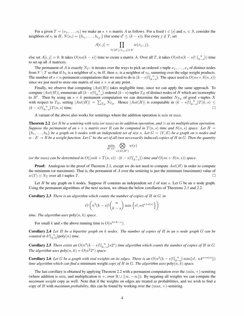
For a given T = (v1, . . . , vt) we make an s× n matrix A as follows. For a fixed i ∈ [s] and si ∈ S, consider theneighbors of si in H , N(si) = hi1 , . . . , hid′ (for some d′ ≤ (k − s)). For every j /∈ T , set

A[i, j] =∏

`∈[d′],(vi` ,j)∈E

w(vi` , j),

else set A[i, j] = 0. It takes O(ns(k − s)) time to create a matrix A. Over all T , it takes O(nks(k − s)!(nk−s)) time

to set up all A matrices.The permanent of A is exactly NT : it iterates over the ways to pick an ordered s-tuple x1, . . . , xs of distinct nodes

from V \ T so that if hk is a neighbor of si in H , then xi is a neighbor of vk, summing over the edge weight products.The number of s×n permanent computations that we need to do is (k− s)!

(nk−s). The space used is O(ns+S(n, s))

since we just need to store one matrix of size s× n at any point.Finally, we observe that computing |Aut(H)| takes negligible time, since we can apply the same approach. To

compute |Aut(H)|, enumerate all (k−s)!(kk−s)

ordered (k−s)-tuples TH of distinct nodes ofH which are isomorphicto H ′. Then by using an s × k permanent computation we can determine the number NTH

of good s-tuples Xwith respect to TH , setting |Aut(H)| =

∑TH

NTH. Hence |Aut(H)| is computable in (k − s)!

(kk−s)T (k, s) ≤

(k − s)!(nk−s)T (n, s) time.

A variant of the above also works for semirings where the addition operation is min or max.

Theorem 2.2 Let R be a semiring with min (or max) as its addition operation, and⊗ as its multiplication operation.Suppose the permanent of an s × n matrix over R can be computed in T (n, s) time and S(n, s) space. Let H =h1, . . . , hk be a graph on k nodes with an independent set of size s. Let G = (V,E) be a graph on n nodes andw : E → R be a weight function. Let C be the set of all (not necessarily induced) copies of H in G. Then the quantity

minH′∈C

⊗e∈E(H′)

w(e)

(or the max) can be determined in O((snk + T (n, s)) · (k − s)!(nk−s)) time and O(sn+ S(n, s)) space.

Proof: Analogous to the proof of Theorem 2.1, except we do not need to compute Aut(H) in order to computethe minimum (or maximum). That is, the permanent of A over the semiring is just the minimum (maximum) value ofw(T )⊗NT over all t-tuples T .

Let H be any graph on k nodes. Suppose H contains an independent set I of size s. Let G be an n node graph.Using the permanent algorithms of the next section, we obtain the below corollaries of Theorems 2.1 and 2.2.

Corollary 2.3 There is an algorithm which counts the number of copies of H in G, in

O

(n2(k − s)!

(n

k − s

)min

s!, n4s+o(s)

)time. The algorithm uses poly(n, k) space.

For small k and s the above running time is O(n3+k−s).

Corollary 2.4 Let H be a bipartite graph on k nodes. The number of copies of H in an n node graph G can becounted in k!

(nk/2

)poly(n) time.

Corollary 2.5 There exists an O(n3(k − s)!(nk−s)s2s) time algorithm which counts the number of copies of H in G.

The algorithm uses poly(n, k) +O(n22s) space.

Corollary 2.6 Let G be a graph with real weights on its edges. There is an O(n2(k − s)!(nk−s)

mins!, n4s+o(s))time algorithm which can find a minimum weight copy of H in G. The algorithm uses poly(n, k) space.

The last corollary is obtained by applying Theorem 2.2 with a permanent computation over the (min,+)-semiring(where addition is min, and multiplication is +, over R ∪ ∞,−∞). By negating all weights we can compute themaximum weight copy as well. Note that if the weights on edges are treated as probabilities, and we wish to find acopy of H with maximum probability, this can be found by working over the (max,×)-semiring.

4

2.1 Computing Permanents of Rectangular Matrices

We now investigate the problem of computing the permanent on matrices with a small number of rows. The bestknown algorithm for computing the permanent is very old, due to Ryser [40]. He gives a formula based on inclusion-exclusion that computes the permanent of an n × n matrix over a ring in O(2npoly(n)) time and O(poly(n)) space.There are two downsides to his algorithm (other than its high running time). First, it cannot be feasibly applied toalgebraic structures without subtraction, due to its use of the inclusion-exclusion principle.2 Secondly, when one triesto generalize the formula to k × n matrices, one only obtains an O(

(nk

)poly(n)) time algorithm (this is well-known

folklore, cf. [34], Section 7.2). Both of these prevent us from using Ryser’s algorithm in the algorithms of the previoussection. Kawabata and Tarui [28] have given a k×n permanent algorithm over rings that runs inO(2kn+3k) time andO(2k) space, by exploiting the Binet-Minc formula for the permanent [34]. In this section, we present new algorithmsthat work over commutative semirings and run in FPT time with respect to k.

Over the integers, the permanent of a k × n Boolean matrix counts the number of matchings in a bipartite graphwith one partition of size k and the other of size n. The more general #k-MATCHING problem is to count the numberof matchings on k nodes in an n node graph. It is a major open problem in parameterized complexity to determine if#k-MATCHING is FPT or if it isW [1]-hard [21]. We do not resolve the complete problem here, but our results do showthat for some bipartite graphs (with f(k) vertices in one partition, for some function f ) the problem is fixed-parametertractable. Our results also imply a 2k+o(k)

(nk/2

)poly(n) time, polynomial space algorithm for #k-MATCHING.

Theorem 2.7 The permanent of a k × n matrix A can be computed in O(k! · kn2) operations over any finite commu-tative semiring.

Note that we count time in terms of the number of plus and times operations over the semiring along with otherbasic machine instructions, and we count space in terms of the total number of elements of the semiring that need tobe stored at any given point in the computation.

Proof: For a k × n matrix A where k ≤ n, we have

perm(A) =∑

f :[k]→[n]f is 1-1

(k∏i=1

A[i, f(i)]

).

Our permanent algorithm tries all possible permutations π : [k]→ [k] of the rows inA. LetAπ be the resulting matrix.A function f on [k] is increasing if f(i+ 1) > f(i) for all i = 1, . . . , k − 1. Given π, define

perm∗(A) =∑

f is increasing

(k∏i=1

A[i, f(i)]

).

Observe thatperm(A) =

∑π

perm∗(Aπ),

since for any one-to-one f there is a unique permutation π on [k] such that f ′ with f ′(i) = f(π(i)) is increasing.We now show how to compute each perm∗(Aπ) efficiently. Make a layered DAG having k layers and at most n

nodes per layer. We include a node labelled j in layer i if and only if Aπ[i, j] 6= 0. Give the node labelled j in layer ia weight of Aπ[i, j]. Now from layer i to layer i+ 1, put arcs from all nodes labelled j to all nodes labelled j′, for allj < j′.

Finally, we need to sum the weights of all k-paths in this DAG, where a path with node weights w1, . . . , wk issaid to have weight

∏ki=1 wi. Note this sum is precisely perm∗(Aπ). The idea is to process the nodes in topological

order and do dynamic programming. At each node v, we maintain the weight W vi of all i-paths that end with v, for all

i = 1, . . . , k. Observe when v has indegree 0, computing W vi is trivial. For an arbitrary node v, we may assume that

2It is possible to apply the algorithm to structures like the (min,+)-semiring by embedding that structure in the ring, but such embeddingsrequire an exponential blowup in the representations of elements in the semiring, cf. Romani [39], Yuval [50].

5

we have already computed the values Wui , for all nodes u with arcs to v. Let the nodes with arcs to v be v1, . . . , vd

and let w(v) be the weight of node v. Clearly, W v1 = w(v). For every i = 1, ..., k − 1, compute

W vi+1 =

d∑j=1

Wvji

· w(v).

When this process completes, we have the weights of all k-paths that end in each node v. It follows that perm∗(Aπ) =∑vW

vk .

We can improve the dependence on k by using recursion.

Theorem 2.8 The permanent of a k × n matrix can be computed in O(4k+o(k)n3) time and O(kn2) space over anycommutative semiring.

Proof: Let A be the matrix. The idea is to try all possible partitions of [k] into sets L and R of cardinality bk/2cand dk/2e respectively, performing a recursive call on an |L| × n and an |R| × n submatrix (one indexed by L, oneindexed by R) which returns all the information we need to reconstruct the permanent. More precisely, let j1 ≤ j2and define Aj1,j2L to be the |L| × |j2 − j1 + 1| submatrix of A with rows indexed by L and columns ranging from thej1th column of A to the j2th column of A. Note A = A1,n

[k] . Let

Bj1,j2L =∑`∈L

A[`, j2] · perm(Aj1,j2−1L\` ), and

Cj1,j2L =∑`∈L

A[`, j1] · perm(Aj1+1,j2L\` ).

Let L be the set of sets L with L ⊆ [k] and |L| = bk/2c. The following identity is the key to the algorithm.

Claim 2.9perm(A) =

∑L∈L

∑1≤j2<j3≤n

B1,j2L · Cj3,n|k|−L.

Proof: Note that on the right hand side, we have∑L∈L

∑1≤j2<j3≤nB

1,j2L · Cj3,n|k|−L =

∑L∈L

1≤j2<j3≤n`∈L,`′∈[k]−L

A[`, j2]·A[`′, j3]·

∑f :(L\`)→1,...,j2−1

f is 1-1

∏i∈L\`

A[i, f(i)]

·

∑f :([k]\L∪`′)→j3+1,...,n

f is 1-1

∏i∈[k]\L∪`′

A[i, f(i)]

.

By distributivity, this sum is

=∑L∈L

∑1≤j2<j3≤n`∈L,`′∈[k]−L

∑

f :L−`→1,...,j2−1f :([k]−L−`′)→j3+1,...,nf(`)=j2,f(`′)=j3,f is 1-1

∏i

A[i, f(i)]

=∑L∈L

∑f :[k]→1,...,n is 1-1∀i∈L,j /∈L f(i)<f(j)

(k∏i=1

A[i, f(i)]

) .

But every one-to-one f fits the condition under the inner sum, for exactly one L of size bk/2c. So the above is just

∑f :[k]→[n]f is 1-1

(k∏i=1

A[i, f(i)]

)= perm(A).

6

More generally, for all i, j, perm(Ai,j[k]) can be expressed as a sum of products of permanents perm(Ai,j2L−`) ·perm(Aj3,j[k]−L−`′). This completes the proof.

We give a simple algorithm PERMANENT to recursively compute perm(A) using the claim. In particular, given ak× n matrix A, the algorithm returns an n× n matrix M where M [i, j] = perm(Ai,j[k]). Hence M [1, n] = perm(A).

PERMANENT(A):If k = 1 then

Return n× n M with M [i, j] =∑`:i≤`≤j A[1, `]

M := the n× n matrix of all zeroesFor all L ⊆ [k] with |L| = bk/2c:

BL, CL := the n× n matrix of all zeroesFor all ` ∈ L:

ML−` := PERMANENT(A1,nL−`).

For all i, j2 ∈ [n]:BL[i, j2] := BL[i, j2] +A[`, j2] ·ML−`[i, j2 − 1].

For all `′ ∈ [k]− L:M[k]−L−`′ := PERMANENT(A1,n

[k]−L−`′).For all j3, j ∈ [n]:

CL[j3, j] := CL[j3, j] +A[`′, j3] ·M[k]−L−`′[j3 + 1, j].M ′ := n× n matrixFor all i, j ∈ [n]:

M ′[i, j] :=∑j2,j3:i≤j2<j3≤j BL[i, j2] · CL[j3, j]

M := M +M ′.Return M .

The correctness of PERMANENT follows from Claim 2.9. A naive way to construct the matrix M ′ of the algorithmrequires Θ(n4) time. To implement it in O(n3), first compute for all i, j, `, NL[i, `] =

∑`x=iBL[i, x] and NR[`, j] =

CR[` + 1, j] whenever ` < j and NR[`, j] = 0 otherwise. Via dynamic programming, building up NR and NL takesonly O(n2) operations. We claim that M = NL · NR where the matrix product is over the semiring. Indeed, for alli, j we have ∑

`

NL[i, `] ·NR[`, j]

=∑

`: i≤`≤j

(BL[i, i] + · · ·+BL[i, `]) · CR[`+ 1, j]

=∑

`1,`2:i≤`1<`2≤j

BL[i, `1] · CR[`2, j] = M ′[i, j].

The runtime recurrence is

T (k) ≤ k(

k

dk/2e

)(T (k/2) +O(n3)

),

yielding T (k) ≤ O(klog k4kn3). The space bound holds, since only O(n2) semiring elements are stored in eachrecursive call.

We remark that Gurevich and Shelah [26] gave a 4npoly(n) algorithm for solving TSP, by trying all partitions ofthe vertices into two halves and recursing. In retrospect, the above approach is similar in spirit.

Finally, we can obtain a faster permanent algorithm over rings. While it also uses exponential space, it stillexponentially improves on Kawabata and Tarui’s algorithm [28]. We require a lemma which is a simple extension ofthe fast subset convolution of Bjorklund et al. [12].

Lemma 2.10 Let N be a positive integer and R be a ring. Let f be a function from the subsets of [N ] of size bK/2cto R and let g be a function from the subsets of [N ] of size dK/2e to R. Suppose we are given oracle access to f and

7

g. Consider h which is a function on the subsets of [N ] of size K to R and is defined as follows:

h(S) =∑

L: |L|=bK/2c

f(L) · g(S − L).

Then one can compute h(S) for all S ⊂ [N ], |S| = K in overall O(K2N ) time and space.

Proof: For any subset X ⊆ [N ] of size ≤ K, define

X0 = T ⊆ X | |T | = bK/2c, and X1 = T ⊆ X | |T | = dK/2e,

f(X) =∑T∈X0

f(T ), and g(X) =∑T∈X1

g(T ).

Let S ⊆ [N ], |S| = K. Consider∑X⊆S

(−1)|S\X| · f(X) · g(X) =∑X⊆S

(−1)|S\X| ·∑

U∈X0,T∈X1

f(U)g(T ) =

=

∑U∈S0,T∈S1

U∩T=∅

(−1)0f(U)g(T )

+

K∑r=1

∑U∈S0,T∈S1

|U∩T |=r

f(U)g(T )

r∑i=0

(r

i

)(−1)r−i

=

=∑U∈S0

f(U)g(S \ U) +

K∑r=1

∑U∈S0,T∈S1

|U∩T |=r

f(U)g(T ) · (−1 + 1)r =∑U∈S0

f(U)g(S \ U).

Let h be the function with h(X) = f(X) · g(X) for all X ⊆ [n], |X| ≤ K.To compute h(S) =

∑U∈S0 f(U)g(S \ U) for all S ⊆ [N ] with |S| = K in O(K2N ) time, it suffices to be able

to compute

1. f(X), g(X) for all X ⊆ [N ] and |X| ≤ K in O(K2N ) time, and

2. given all h(X),∑X⊆S(−1)|S\X|h(X) in O(K2N ) time.

We will first show how to compute f(X) in O(K2N ) time: Iterate over all s from 1 to N and over all sets X ofsize ≤ K containing s. For each fixed s and X , let s′ be the largest element of X smaller than s, and set

fs(X) = fs′(X \ s) + fs′(X).

We initialize for each X ⊆ [N ]

f0(X) =

f(X) if |X| = bK/2c0 otherwise.

The runtime of this procedure is O(K(NK

)) = O(K2N ) as every set X is accessed at most |X| + 1 times and

|X| ≤ K. The final result is f(X) = fN (X). Computing g(X) is analogous. To obtain h(S), simply go through allS in O(2N ) time and set h(S) = f(S) · g(S).

Computing∑X⊆S(−1)|S\X|h(X) given all h(X) proceeds similarly to above: Iterate over all s from 1 to N and

over all sets X of size ≤ K containing s. For each fixed s and X , let s′ be the largest element of X smaller than s,and set

hs(X) = −hs′(X \ s) + hs′(X).

We initialize for each X ⊆ [N ], h0(X) = h(X). The runtime of this procedure is also O(K2N ) as every set X isaccessed at most |X|+ 1 times and |X| ≤ K. The final result is hN (S).

8

Theorem 2.11 The permanent of a k × n matrix over any ring can be computed in O(kn32k) time and O(n22k)space.

Proof: We use the formula from Claim 2.9 from the proof of Theorem 2.8.Suppose that perm(Aj1,j2T ) is known for all j1, j2 ∈ [n] and all sets T of size bk/2ic − 1, bk/2ic − 2, bk/2ic − 3.

Then for all sets L of size bk/2ic, bk/2ic − 1, bk/2ic − 2, Bj1,j2L and Cj1,j2L can be computed in O(kn22k/2i) time.Consider Aj1,j2S for S of size bk/2i−1c − 1, bk/2i−1c − 2, bk/2i−1c − 3. From Claim 2.9 we have:

perm(Aj1,j2S ) =∑L⊆S

|L|=b|S|/2c

∑j1≤p2<p3≤j2

Bj1,p2L · Cp3,j2S−L .

The size b|S|/2c is bk/2ic, bk/2ic − 1, or bk/2ic − 2, and d|S|/2e is bk/2ic or bk/2ic − 1. The values for Bj1,p2L

and Cp3,j2L for L of such sizes have been computed and stored. By computing NL and NR as in the previous theorem,and swapping the order of the sums in the resulting expression, we can use the fast subset convolution of Lemma 2.10to compute perm(Aj1,j2S ) in O(n3k2k/2i) time, for all S of size bk/2i−1c − 1, bk/2i−1c − 2, or bk/2i−1c − 3, andj1, j2 ∈ [n].

Therefore computing perm(A) takes O(∑log ki=0 kn32k−i) = O(kn32k) time. The space usage is O(n22k) since

at each stage we need to store O(n22k) values.

Subsequent Work Since the conference version of this paper appeared, there has been subsequent work on comput-ing permanents of rectangular matrices. Recently, Bjorklund et al. [11] have obtained several algorithms for computingthe permanent of a k× n matrix over semirings and rings. Let

(n↓s)

=∑st=0

(nt

). Bjorklund et al. show that the k× n

permanent can be computed in

• O(k ·(n↓k)) time and O(

(n↓k)) space over any semiring,

• in O(kn2k) time and space over any commutative semiring,

• in O(k(n↓k/2

)) time, and O(

(n↓k/2

)) space over any ring, and

• in O(kn2k) time and O(n) space over any commutative ring.

Koutis and Williams [31] also give an O(2kpoly(n)) time and space algorithm for the k × n permanent over commu-tative semirings, and an O(2kpoly(n)) time and polynomial space algorithm over commutative rings.

3 Counting Weighted Patterns

In the following, we assume k = |H| is divisible by 3. However our results trivially extend to all k, with possibly anextra factor of n or n2 in the running time. The weight of a subgraph is defined to be the sum of its node (or edge)weights. A graph has K-weight if its weight is K.

The algorithms in the previous section can find a maximum (or minimum) weight H-subgraph in a given G. Theycan be extended to count maximum weight subgraphs if the weights in G are bounded. However, it is unclear how toextend the results of the previous section for counting general weighted subgraphs H .

There has been a lot of recent work in finding weightedH-subgraphs in node-weighted graphs ([46, 47, 19]). Thereare several versions of the problem: (1) find a maximum (or minimum) weight H-subgraph, (2) find an H-subgraphof weight at least K for a given K, and (3) find a K-weight H-subgraph for a given weight K. The idea which hasbeen used in attacking all three versions of the problem is that each version can be reduced to finding a weighted(maximum, at least K, or K-weight) triangle in a larger node-weighted graph. If such a triangle can be found inT (n) time and S(n) space in an n node graph, then the corresponding weighted H-subgraph problem can be solvedin O(k2T (nk/3)) time and O(S(nk/3)) space. The same reduction works for counting H-subgraphs: if the weightedtriangles in an n node graph can be counted in T (n) time and S(n) space, then the weighted H-subgraphs can be

9

counted in O(k2T (nk/3)) time and O(S(nk/3)) space. Here we take a similar approach, and study the correspondingtriangle problems.

In previous work [46] we showed that the triangles of weight at least K in a node-weighted graph on n nodes canbe counted in O(n

3+ω2 ) time. The same approach yielded an O(n

3+ω2 ) runtime for counting K-weight triangles. By

binary searching on K, this gave a way to count the maximum weight triangles in a node-weighted graph in O(n3+ω2 )

time. This in turn implied an O(n0.896k) running time for counting weighted H-subgraphs (for any of the threeversions of the problem), and constituted the first nontrivial improvement over the brute force O(nk) runtime.

Czumaj and Lingas [19] used an interesting technique to show that a maximum weight triangle can be found inO(nω + n2+ε) time for all ε > 0. Their method is based on a combinatorial lemma which bounds the number oftriples in a set where no triple strictly dominates another.

Lemma 3.1 (Czumaj and Lingas [19]) Let U be a subset of 1, . . . , n3. If there is no pair of points (u1, u2, u3),(v1, v2, v3) ∈ U such that uj > vj for all j = 1, 2, 3, then |U | ≤ 3n2.

Similarly to Czumaj and Lingas’ approach in [19], we show that Lemma 3.1 can be used to solve all three versionsof the weighted triangle problem in node-weighted graphs. Furthermore, it can be used to count node-weightedtriangles in nω+o(1) time, improving on the O(n(3+ω)/2) time solution. The new algorithm immediately implies anO(nωk + n(2+ε)k) for every ε > 0 running time for counting weighted subgraph patterns on 3k nodes in an n-vertexnode-weighted graph. We prove the result for counting exact node-weighted triangles. Counting maximum weighttriangles or triangles of weight at least K can be done similarly, hence we omit those algorithms.

Theorem 3.2 Let G = (V,E) be a given n node graph with weight function w : V → R. Let K ∈ R be given. Thenin n2 ·exp(O(

√log n))+O(nω) time one can compute for every pair of vertices i, j the number ofK-weight triangles

that include the edge (i, j). Furthermore, for every (i, j) in a K-weight triangle, the algorithm can find a witnessnode k such that i, j, k form a K-weight triangle. The witness computation incurs only a polylogarithmic factor in theruntime.

Proof: Create a global n× n output matrix D that is initially zero. After the completion of the algorithm, D[i, j]will contain the number of K-weight triangles that include i and j.

Sort the vertices in nondecreasing order of their weights in O(n log n) time. We build three identical sorted listsA,B,C of the n nodes. Our algorithm counts all triangles with a single node in each of A, B, and C.

The algorithm is recursive, and its input is three sorted lists of nodes A,B,C each having at most N nodes. Thealgorithm does not return information, but rather adds numbers to D when the recursion bottoms out.

Let c be a parameter. Sort A, B and C (in nondecreasing order) and partition them into c sublists A1, . . . , Ac,B1, . . . , Bc, C1, . . . , Cc of at most dN/ce nodes each, as follows. If A = (a1, . . . , aN ), then for each 0 ≤ i <c− 1, let Ai+1 = (aidN/ce+1, . . . , a(i+1)dN/ce) . B and C are split similarly. Each new sublist is now associated withthe interval of weights between the smallest and largest weights of its nodes.

For each 1 ≤ i < c and each 1 ≤ k ≤ dN/ce, let Ai[k] refer to the k-th element of Ai in the sorted order. DefineBi[k], Ci[k] similarly.

Consider all c3 triples (Ai, Bj , Ck). Let [ai, a′i], [bj , b

′j ] and [ck, c

′k] be the weight intervals for Ai, Bj , and Ck,

respectively.

Case 1: ai = a′i or bj = b′j , or ck = c′k. This case represents the bottom of the recursion. If bj = b′j , then create twomatrices X and Y , defined as:

X[p, q] =

1 if (Ai[p], Bj [q]) ∈ E,0 otherwise, and

Y [q, r] =

1 if (Bj [q], Ck[r]) ∈ E,0 otherwise.

Multiply X and Y . For all p, q with w(Ai[p]) + w(Ck[q]) = K − bj and (Ai[p], Ck[q]) ∈ E, the entry(XY )[p, q] gives the number of nodes in Bj which form a K-weight triangle with Ai[p] and Ck[q]. Add (XY )[p, q]to D[Ai[p], Ck[q]].

10

The cases ai = a′i and ck = c′k are symmetric. Without loss of generality, assume ai = a′i. Then create twomatrices X and Y as follows:

X[p, q] =

1 if (Ai[p], Bj [q]) ∈ E0 otherwise.

Y [q, r] =

1 if (Bj [q], Ck[r]) ∈ E and

w(Bj [q]) + w(Ck[r]) = K − ai,0 otherwise.

Multiply X and Y . For every p, q with (Ai[p], Ck[q]) ∈ E, the entry (XY )[p, q] gives the number of nodes in Bjwhich form a K-weight triangle with Ai[p] and Ck[q]. Add (XY )[p, q] to D[Ai[p], Ck[q]].

In both cases above, one can find witnesses and incur only a polylogarithmic factor by using the Boolean matrixproduct witness algorithm of Alon et al. [3].

Case 2: ai < a′i and bj < b′j , and ck < c′k. Recurse on all triples (Ai, Bj , Ck) with intervals [ai, a′i], [bj , b

′j ], [ck, c

′k]

satisfyingai + bj + ck ≤ K ≤ a′i + b′j + c′k.

Note we can disregard all other triples of nodes, as they could not contain a K-weight triangle with a node in each ofAi, Bj , and Ck. This concludes the algorithm.

Observe that we only add to D when the recursion bottoms out, and at least one sublist has the same weight on allof its nodes. Because of the partitioning, we never overcount, and every triangle of weight K is counted exactly once.

We claim that the number of recursive calls in the algorithm is at most 6c2. There are two types of triples that thealgorithm recurses on: those with ai+bj+ck ≤ K < a′i+b

′j+c

′k (type 1) and those with ai+bj+ck < K ≤ a′i+b′j+c′k

(type 2). Let T1 and T2 be the sets of type 1 and type 2 triples respectively. We show that |Ti| ≤ 3c2 for i = 1, 2.Each triple in T1 is uniquely determined by the three left endpoints of its weight intervals, (ai, bj , ck). This follows

since ai < a′i, bj < b′j and cj < c′j . Similarly, each triple in T2 is uniquely determined by the three right endpoints ofits weight intervals, (a′i, b

′j , c′k).

To prove that |T1| ≤ 3c2, let (Ai, Bj , Ck) ∈ T1 and consider any (A`, Bp, Cq) with ai < a`, bj < bp and ck < cq .Because of the way we partitioned A,B,C, we must have a′i ≤ a`, b′j ≤ bp and c′k ≤ cq . Hence

ai + bj + ck ≤ K < a′i + b′j + c′k ≤ a` + bp + cq,

and therefore (A`, Bp, Cq) /∈ T1. That is, no triple in T1 is strictly dominated by another one. By Lemma 3.1 thereare at most 3c2 triples in T1. The argument for T2 is symmetric.

The time recurrence has the form:

T (n) ≤ 6c2T (n/c) + dc3(n/c)ω,

for a constant d.Czumaj and Lingas [19] showed that a similar recurrence solves to O(nω + n2+ε) for all ε > 0. We improve

their analysis by proving that c can be chosen (depending on ω) so that the recurrence solves to T (n) ≤ O(nω) +n22O(

√logn).

If ω > 2, pick any ε with 0 < ε < ω − 2 and set c = 61/ε (we can pick ε so that c is an integer). By the mastertheorem (see e.g. [17]), if 2 + ε = (log 6 + 2 log c)/(log c) < ω and for some c′′ < 1, 6c2(n/c)ω ≤ c′′nω then theruntime is O(nω). Now 6c2(n/c)ω = 6nω/cω−2 = nω · 61−ω−2

ε , and 61−ω−2ε < 61−1 = 1. Hence in this case the

runtime is precisely O(nω).Suppose ω = 2. Set c(n) = 2p

√logn for some constant p > 7. Let q = p

2 − ε for some 0 < ε < 1/2. Let

c′′ = 2qc′

2q−6 and notice c′′ > c′ > 0 and q = log(

6c′′

c′′−c′

).

For large enough n,

q2 − 2ε

√log n− p

√log n < 0, and

(

√log n− p

√log n+ q)2 = (log n− p

√log n) + (p− 2ε)

√log n− p

√log n+ q2 ≤

11

log n+ q2 − 2ε

√log n− p

√log n < log n.

Hence,√

log n− p√

log n+ q <√

log n. Substituting q = log 6c′′

c′′−c′ , p√

log n = log c and multiplying by p,

log(6c′′) + p

√log

n

c< p√

log n+ log(c′′ − c′).

Raising 2 to the power of each side, adding cc′ to both sides and then multiplying both sides by n2, we obtain

n2(6c′′ · 2p√

log(n/c) + cc′) < c′′n22p√

logn.

By the induction hypothesis, however, the left hand side is at least 6c2T (n/c) + c′c3(n2/c2) ≥ T (n). We get thatT (n) ≤ c′′n22p

√logn and hence by induction our algorithm takes n2 · 2O(

√logn) time.

Theorem 3.2 can be viewed as an efficient reduction from counting node-weighted triangles to counting un-weighted triangles. However the reduction does not preserve the sparsity of the original graph, and hence a verygood algorithm for counting/finding triangles in a sparse unweighted graph does not necessarily imply an algorithmwith a comparable running time for node-weighted graphs3. Furthermore, because of the sorting, the method used inTheorem 3.2 would require linear space to solve weighted triangle problems in truly subcubic time. Note however,that there may be an algorithm for triangle finding which runs in O(n3−ε) time and uses no(1) space; the trivial O(n3)time algorithm uses only O(log n) space. With the reduction in Theorem 3.2 such an algorithm would not translateto a small space subcubic algorithm for node-weighted triangle finding. The linear space usage of the reduction alsomeans that the corresponding reduction from counting or finding weighted H-subgraphs to counting or finding trian-gles would require nΩ(k) space. To resolve these issues, we give a completely different construction which reducesthe problem of finding a weighted triangle to a small number of instances of finding unweighted triangles in graphswith the same number of nodes and edges.

We first observe that all versions of the weighted triangle existence problems can be reduced to the K-weight(exact weight) case with a poly(logW ) runtime overhead, where W is the maximum weight in the graph. Hence wecan concentrate on the exact weight case.

Theorem 3.3 Suppose there is a T (m,n,W ) time and S(m,n,W ) space algorithm which determines if there is atriangle of weight 0, in an node or edge weighted graph on n nodes and m edges with maximum weight W . Let Kbe any integer. Then given an n-node m-edge graph with node or edge weights at most W , there are O(S(m,n,W ))space algorithms for finding a triangle of weight at least K and for finding a maximum weight triangle, with timeO(T (m,n,W ) logW ) and O(T (m,n,W ) log2W ), respectively.

Given a B-bit integer x we define prei(x), the ith prefix of x, to be the integer obtained from x by removing thelast B − i bits of x. We will use prei(x) to denote both the prefix integer and its representation as a bit sequence. Theproof of Theorem 3.3 relies on Proposition 3.4 below. We use Proposition 3.4 to process the integer weights in a givenweighted triangle instance by creating new instances of 0-weight triangle in which the weights are the prefices prei(·)for some i, or the prefices concatenated with a single bit, as in prei(x)1 or prei(x)0.

Proposition 3.4 For three integers x, y, z we have that x+ y > z, if and only if one of the following holds:

• there exists an i such that prei(x) + prei(y) = prei(z) + 1, or

• there exists an i such that prei+1(x) = prei(x)1, prei+1(y) = prei(y)1, prei+1(z) = prei(z)0 and prei(x) +prei(y) = prei(z).

Proof: If one of the two conditions holds, we clearly have x+ y > z. We only need to prove the opposite direction.Suppose x+ y > z. Then there exists some i with prei(x) + prei(y) ≥ prei(z) + 1. Consider the smallest such i. Ifprei(x) + prei(y) = prei(z) + 1, then we are done, so assume prei(x) + prei(y) ≥ prei(z) + 2. Then we have that

3We note that an O(m1.41) runtime for counting weighted triangles is possible using the high degree/low degree method of Alon, Yuster, andZwick [5].

12

prei−1(x) + prei−1(y) ≤ prei−1(z). For some b1, b2, b3 ∈ 0, 1, prei(x) = prei−1(x)b1, prei(y) = prei−1(y)b2and prei(z) = prei−1(z)b3, and

2(prei−1(x) + prei−1(y)) + 2 ≥ 2(prei−1(x) + prei−1(y)) + b1 + b2 ≥ prei(z) + 2 =

2prei−1(z) + b3 + 2 ≥ 2(prei−1(x) + prei−1(y)) + 2 + b3.

Hence we have that b3 = 0, b1 = b2 = 1 and prei−1(x) + prei−1(y) = prei−1(z).

Now we can prove the Theorem:Proof of Theorem 3.3. The maximum weight triangle problem can be reduced to the > K-weight triangle problemjust by binary searching for the maximum weight. This incurs an overhead of logW in the running time and no spaceoverhead. Hence we just reduce the > K-weight triangle problem to the 0-weight triangle problem. We assume thatwe have a T (m,n,W ) time, S(m,n,W ) space algorithm which can find a triangle of weight exactly 0 if one exists.Given this algorithm it is straightforward to obtain an O(T (m,n,W )) time, O(S(m,n,W )) algorithm which finds atriangle of weight K for any given K. We will give a procedure which given K, determines whether there is a trianglein the graph of weight sum > K. We give the reduction for edge weighted graphs. The node-weighted graph case issimilar.

Implicitly build a tripartite graph G′ = (V ′, E′) from G = (V,E) by creating three copies V1, V2, V3 of the vertexset V and set V ′ = V1 ∪ V2 ∪ V3. For every u ∈ V , let ui denote its copy in Vi. Then E′ = (ui, vj) | (u, v) ∈E, i, j ∈ 1, 2, 3, i 6= j. LetW = maxu,v |w(u, v)|. We set up the weightsw′ forG′ as follows: we letw′(u1, vj) =w(u, v) + W for j ∈ 2, 3 and w′(u2, v3) = 2W + K − w(u, v). Now, a triangle a1, b2, c3 with the property thatw′(a1, b2) + w′(a1, c3) > w′(b2, c3) exists in G′ iff there is a triangle a, b, c in G of weight sum > K. To create aprocedure which determines whether there is such a triangle in G′ we use Proposition 3.4.

The integers in G′ have O(logW ) bits. We create O(logW ) instances of 0–weight triangle as follows. For everyprefix i = 0, . . . , O(logW ) create two instances of 0-weight triangle Gi1 and Gi2.

For every (uj , vk) ∈ E′, (uj , vk) is also an edge in Gi1 with weight prei(w′(uj , vk)) if j = 1 and k ∈ 2, 3 andwith weight −prei(w′(uj , vk))− 1 otherwise. This corresponds to the first bullet of Proposition 3.4.

For every (uj , vk) ∈ E′, (uj , vk) is an edge in Gi2 if j = 1 and prei+1(w′(uj , vk)) = prei(w′(uj , vk))1, or

if j = 2, k = 3 and prei+1(w′(uj , vk)) = prei(w′(uj , vk))0. The weight of (uj , vk) in Gi2 is prei(w′(uj , vk)) if

j = 1 and −prei(w′(uj , vk)) otherwise. This corresponds to the second bullet of Proposition 3.4.By Proposition 3.4, there is a triangle with weight > K in G if and only if for some i ∈ 0, . . . , O(logW ) and

b ∈ 1, 2, the graph Gib contains a 0-weight triangle.We note that we do not need to explicitly construct the graphsGib. Whenever the 0-weight triangle algorithm needs

to know whether a particular edge exists and (if so) what its weight is, we compute this by checking the adjacencymatrix of the original graph. Hence there is no space overhead.

We now give a tight reduction from node-weighted triangle finding to triangle finding which is both time and spaceefficient.

Theorem 3.5 Suppose there is a T (m,n) time, S(m,n) space algorithm which finds a triangle in an n-node, m-edgegraph, or determines that the graph is triangle-free. Let K be any integer. Then there is a T (m,n) · 2O(

√logW )

time, O(S(m,n)) space randomized algorithm which finds a K-weight triangle in an n node m edge graph with nodeweights in [1,W ], or determines that such a triangle does not exist, with high probability at least 1− 1/poly(W ).

Our method relies on the existence of a good three-party communication protocol for Exactly-W . Exactly-W isthe multiparty communication problem where w ∈ [W ] is known to all parties, the ith party has an integer ni ∈ [1,W ]on its forehead and can thus see all nj but ni; all parties wish to determine if

∑i ni = w. This problem was

defined by Chandra, Furst, and Lipton [13]. They showed that Exactly-W has three-party communication complexityO(√

logW ), but they did not give an effectively computable version of their protocol. We show how to modify theprotocol so that it can be used to obtain a fast exact triangle algorithm. A crucial aspect of the protocol is that it doesnot have false positives: if the sum is not w then it always rejects.

Theorem 3.6 Exactly-W has a simultaneous randomized three-party protocol withO(√

logW ) communication com-plexity, where each party runs a 2O(

√logW ) time algorithm and has access to 2O(

√logW ) public random bits. In

13

particular, consider an instance (w1, w2, w3) ∈ [W ] of Exactly-W for three parties. If w1 + w2 + w3 = w then theprotocol accepts with probability at least 1− 1/poly(W ), and if w1 +w2 +w3 6= w then the protocol always rejects.

We note that by making the acceptance probability 1/2Ω(√

logW ), one can easily modify the protocol of Theo-rem 3.6 so that it has O(1) communication complexity, and each party runs a poly(logW ) time algorithm and hasaccess to 2 logW public random bits.

Proof: Let us survey the protocol in [13], then describe how to adapt it. Their protocol is deterministic, usesO(√

logW ) bits of communication, and is non-constructive. At the heart of the protocol is a “hash” function h(x)from [W ] to [k], where k << W , which we now describe. Let S ⊆ [W ] be 3-AP-free, meaning that it contains noarithmetic progression of length three. It is known that for all W , there is a constant c > 0 and 3-AP-free set S ⊆ [W ]of size cW/2c

√logW . Consider a random translate of S, i.e. a set of the form Si = x + yi | x ∈ S for a uniform

random yi ∈ −W, . . . ,W. The set [W ] is covered by k ≤ O(W|S| logW ) ≤ O(2c√

logW logW ) random translatesS1, . . . , Sk with probability at least 1− 1/poly(W ), where each |Si| = |S|, and each Si is 3-AP-free. For x ∈ [W ],define h(x) to be the smallest i ∈ [k] such that x ∈ Si.

Now we describe the protocol. Each party holds two of the wi ∈ [W ] (along with knowledge of w) and wants toknow if w1 + w2 + w3 = w. Observe that each party “knows” what its missing number ought to be if the sum is w,for example the party holding w1 and w2 knows that w3 should be w − w1 − w2. The ith party computes its ownxi = w1 + 2w2 + 3w3, using the difference between w and its two known integers in place of its missing integer, thensends h(xi) using O(log(W/|S|)) bits. We claim that w1 + w2 + w3 = w if and only if h(x1) = h(x2) = h(x3), sothe protocol accepts if and only if all messages are identical. If w1 + w2 + w3 = w, then obviously x1 = x2 = x3. Ifw1 +w2 +w3 6= w, we claim that x1, x2, x3 is a three-term arithmetic progression; by construction of S, it follows thatnot all h(xi) are equal. Let α = w−w1−w2−w3 6= 0. Then x1 = (w−w2−w3)+2w2+3w3 = (α+w1)+2w2+3w3,x2 = w1 +2(w−w1−w3)+3w3 = w1 +2(α+w2)+w3, x3 = w1 +2w2 +3(α+w3). Letting a = w1 +2w2 +3w3,we have x1 = a+ α, x2 = a+ 2α, x3 = a+ 3α, a progression.

A possible obstacle to obtaining a constructive version of the protocol from [13] described above is the 3-AP-free set S. Behrend [9] (building on Salem and Spencer [41]) gave the first 3-AP-free S of size Ω(W 1−c/

√logW ).

His proof gives a procedure for generating elements of S, but in the above protocol we need to be able to recognizemembers of S; it is not clear how to do this quickly with Behrend’s set. Fortunately, Moser [35] later gave a 3-AP-freeS of comparable size for which membership of a (logW )-bit number x can be determined in O(poly(logW )) time.

Now suppose that each party i can test membership in S, then they could determine h(xi) in 2O(√

logW ) time byenumerating through all 2O(

√logW ) random translates Sj . Then they can easily send log(2O(

√logW )) = O(

√logW )

bits describing h(xi). Using this version of the protocol the three parties can determine whether w1 + w2 + w3 = w,with high probability. The protocol requires 2O(

√logW ) public random bits, O(

√logW ) bits of communication, and

each party runs a 2O(√

logW ) time algorithm.

Proof of Theorem 3.5. Let G = (V,E) be a given graph. Let V = v1, . . . , vn and let G have weights w :V → 1, . . . ,W. We run the following algorithm. Let B = O(

√logW ) be the communication complexity of

the simultaneous protocol in Theorem 3.6. The algorithm cycles over every possible sequence b1, b2, b3, where bj ∈0, 1∗ and |bj | ≤ B for j ∈ 1, 2, 3. These sequences represent all possible simultaneous communications thatcould take place. Note the number of sequences is 2O(

√logW ).

Given a possible communication sequence S, we implicitly construct a graph G′S on 3n nodes. G′S is tripartitewith vertex partitions V 1 = v1

1 , . . . , v1n, V 2 = v2

1 , . . . , v2n, V 3 = v3

1 , . . . , v3n. For i ∈ 1, 2, 3 and k, ` ∈ [n],

there is an edge between vik and vi+1` (the indexing is done mod 3) iff (1) (vk, v`) ∈ E and (2) the ith party accepts

while holding w(vk) and w(v`) and viewing communication sequence S.If one finds a triangle in G′S then the corresponding triangle in G has weight K, by the correctness of the protocol.

If there is a K-weight triangle in G, then with constant nonzero probability there is a triangle in G′S for some S, after2O(√

logW ) runs of the algorithm. We do not need to construct any of the graphs G′S , rather every time we need tocheck whether an edge (vij , v

i+1k ) is in G′S , we run the protocol of Theorem 3.6 for party i in 2O(

√logW ) time, making

sure it matches S.

14

4 Hardness for Edge Weighted Subgraphs

The methods for finding weighted triangles described in the previous section still fail in the edge weighted case. Notruly subcubic algorithms are known for finding a weighted triangle in an edge-weighted graph, for any of the threeversions of the problem we have considered. Finding a maximum weight triangle in truly subcubic time has receivedrecent attention (e.g. [46, 47, 19]) due to its connection to all pairs shortest paths (APSP). This connection has recentlybeen made formal by the authors [48]: a truly subcubic algorithm for maximum weight triangle in an edge-weightedgraph exists if and only if there is a truly subcubic algorithm for APSP. Thus understanding edge-weighted triangleproblems could explain why it seems so difficult to obtain a truly subcubic algorithm for APSP. In this section we relatethe exact version of the edge-weighted triangle problem to 3SUM and the multivariate quadratic equations problem.We say that a triangle in an edge-weighted graph has K-edge-weight if the sum of its edge weights is K.

4.1 3SUM

First we show a connection between findingK-edge-weight triangles and the 3SUM problem, which is widely believedto have no truly subquadratic algorithm (cf. [24]). Our goal is to show that if the K-edge-weight triangle problem canbe solved in truly subcubic time then 3SUM is solvable in truly subquadratic time. We first prove by a direct reductionthat if the K-edge-weight triangle problem can be solved in O(n2.5−ε) time then 3SUM is solvable in O(n2−ε′) time.After this, we use combine our ideas with a recent result by Patrascu [38] to show a tight relationship between the twoproblems.

Theorem 4.1 If for some ε > 0 there is an O(n2.5−ε) algorithm for finding a 0-edge-weight triangle in an n nodegraph, then there is a randomized algorithm which solves 3SUM on n numbers in expected O(n

85 + n2− 4

5 ε) time.

Proof: Suppose we are given an instance (A,B,C) of 3SUM so that A, B and C are sets of n integers each. Wefirst use a hashing scheme given by Dietzfelbinger [20] and used by Baran, Demaine and Patrascu [7] which mapseach distinct integer independently to one of n/m buckets where m is a parameter we will choose later 4. For eachi ∈ [n/m], let Ai, Bi, and Ci be the sets containing the elements hashed to bucket i. The hashing scheme has two niceproperties:

1. for every pair of buckets Ai and Bj there are two buckets Ckij0 and Ckij1 (which can be located in O(1) timegiven i, j) such that if a ∈ Ai and b ∈ Bj , then if a+ b ∈ C then a+ b is in either Ckij0 or Ckij1 ,

2. the number of elements which are mapped to buckets with > 3m elements is O(n/m) in expectation.

After the hashing we process all elements that get mapped to large buckets (size > 3m) as follows. Suppose thata ∈ A is an element mapped to a large bucket. Then go through all elements b of B and check whether a + b ∈ C.Process elements of B and C mapped to large buckets similarly. This takes O(n2/m) time overall in expectation.

Now the buckets Ai, Bi, Ci for all i ∈ [n/m] contain O(m) elements each. For each i ∈ [n/m], pick an arbitraryordering of the elements of Ai and then denote by Ai[k] the kth element in Ai. Similarly, denote by Bi[k] and Ci[k]the kth elements of Bi and Ci.

For every c ∈ [2m] we will create an instance of 0-edge-weight triangle as follows. For every i ∈ [n/m], createnodes xi and yj . For every s ∈ [m] and t ∈ [m] create a node zst. Add an edge (xi, zst) for every i, s, t with weightAi[s]. Add an edge (zst, yj) for every j, s, t with weightBj [t]. For every i, j add an edge (xi, yj) with weight Ckij0 [c]if c ≤ m and Ckij1 [c−m] if c > m.

If in any one of the 2m instances there is a triangle of edge weight 0, then this triangle has the form xi, zst, yj andhence Ai[s], Bj [t], Ckij [c] for some c is a solution to the 3SUM instance. Suppose on the other hand that there is asolution a, b, d of the 3SUM instance. Either we found this solution during the reduction to 0-edge-weight triangle, ora = Ai[k], b = Bj [`] and d = Ckijf [p], for f ∈ 0, 1, k, `, p ∈ 1, . . . ,m, and i, j ∈ 1, . . . , n/m. Then considerinstance c = fm+ p. The triangle xi, yj , zk` has weight Ai[k] +Bj [`] + Ckijf [p] = a+ b+ d.

Each graph has O(n/m+m2) nodes and can be constructed in O(n2/m2 +m4) time. The entire reduction takesO(n2/m + m4) expected time. By setting m = Θ(n1/3) we obtain O(n1/3) instances of 0-edge-weight triangle,

4The scheme performs multiplications with a random number and some bit shifts hence we require that these operations are not too costly. Wecan ensure this by first mapping the numbers down to O(logn) bits, e.g. by computing modulo some sufficiently large Θ(logn) bit prime.

15

each on O(n2/3) nodes. Hence if a 0-edge-weight triangle in an N node graph can be found in O(N2.5−ε) time, then3SUM is in O(n5/3 + n

13 +

(2.5−ε)23 ) = O(n5/3 + n2−ε 2

3 ) time.We note that the reduction can be improved slightly by instead of creating n1/3 instances of size n2/3 we create

one instance of size n4/5. Then an O(n2.5−ε) algorithm for 0-edge-weight triangle would imply an O(n8/5 + n2− 45 ε)

algorithm for 3SUM. To do this, for each i and j create 2√m copies xic and yjc (for c = 1, . . . , 2

√m) of the original

nodes xi and yj . For each c and each node zst the weight of edge (xic, zst) is Ai[s] and that of edge (yjc, zst) is Bj [t].Now there are 4m instances (xic, yjc′) of the original edge (xi, yj) and we can place the 2m numbers of Ckij0 ∪Ckij1on these edges so that each number appears at least once. Now we have one instance onO(n/

√m+m2) nodes created

in O(n2/m+m4) time. By setting m = n2/5 we obtain the result.

Recently, Patrascu [38] gave a reduction from 3SUM to a problem called Convolution-3SUM problem. Combininghis result with our ideas, we show that if one can find a 0–weight triangle in truly subcubic time, then 3SUM can besolved in truly subquadratic time, thus tightening the relationship between the two problems.

Convolution-3SUM problem is the following problem: given arrays A[0 . . . N ], B[0 . . . N ] and C[0 . . . N ], findsome i, j with A[i] +B[j] = C[i+ j].

Theorem 4.2 (Patrascu [38]) If Convolution-3SUM can be solved in O(N2/f(N)) time for some function f , then3SUM can be solved in O(n2/f1/3(n)) time.

Here we give details on how to reduce Convolution-3SUM to 0–weight triangle.

Theorem 4.3 If a 0-edge-weight triangle in a graph on c nodes can be found in T (c) = O(c3/f(c)) time for somefunction f , then Convolution-3SUM on N length arrays can be solved in O(N2/f(

√N)) time time, and 3SUM on n

integers can be solved in O(n2/f1/3(√n)) time.

Proof: Consider an instance A,B,C of Convolution-3SUM of length N . We want to find i, j such that A[i] +B[j] = C[i+ j]. For i ∈ [

√N ], let Ai be the

√N length array with Ai[j] = A[(i− 1)

√N + j], that is we split A up

into consecutive chunks of length√N . We split up B similarly into Bi for i ∈ [

√N ]. For every i ∈ [

√N ] we create

a complete tripartite graph Gi on partitions Li, Ri, Si with√N nodes each. Let Li[t], Ri[t] and Si[t] denote the t-th

node in partition Li, Ri and Si respectively. We add weights to the edges as follows:

• w(Li[s], Ri[t]) = As[t]

• w(Ri[t], Si[q]) = Bi[q − t]

• w(Li[s], Si[q]) = −C[(s+ i− 2)√N + q]

Now, if we find a 0-edge-weight triangle Li[s], Ri[t], Si[q], then

0 = As[t] +Bi[q − t]− C[(s+ i− 2)√N + q],

A[(s− 1)√N + t] +B[(i− 1)

√N + q − t] = C[(s+ i− 2)

√N + q],

and if m1 = (s− 1)√N + t, m2 = (i− 1)

√N + q − t, then

m1 +m2 = (s+ i− 2)√N + q,

and we have found A[m1] +B[m2] = C[m1 +m2].If on the other hand there is somem1,m2,m3 = m1 +m2 such thatA[m1]+B[m2] = C[m1 +m2], then consider

Gi for which m2 = (i − 1)√N + m2 for m2 ∈ 0, . . . ,

√N − 1. Let m1 = (s − 1)

√N + t for 0 ≤ t <

√N .

Consider the edge (Ri[t], Si[m2 + t]). It has weight Bi[m2] = B[m2]. Edge (Li[s], Ri[t]) has weight A[m1] andedge (Li[s], Si[m2 + t]) has weight −C[w] for w = (s+ i− 2)

√N + m2 + t = m1 +m2. Hence there is a triangle

with weight A[m1] +B[m2]− C[m1 +m2] = 0.If a 0-edge-weight triangle in a graph on c nodes can be found in T (c) = O(c3/f(c2)) time, then Convolution-

3SUM on N length arrays can be solved in√NT (

√N) =

√N ·N3/2/f(N) = N2/f(N)

time, and hence 3SUM can be solved in O(n2/f1/3(n)) time.

16

Corollary 4.4 If 0-edge-weight triangle on n node graphs is in O(n3−ε) time, then 3SUM on N integers is inO(N2−ε/6) time.

4.2 Multivariate Quadratic Equations

Finally, we show that faster algorithms for finding edge-weighted triangles would also imply faster algorithms forNP-hard problems. In particular, a better algorithm for exact edge weighted triangle over finite fields could be used tosolve MULTIVARIATE QUADRATIC EQUATIONS (abbreviated as MQS) faster than exhaustive search. An instance ofMQS consists of a set of m equations over n variables that take values from a finite field F , where each equation is ofthe form

p(x1, . . . , xn) = 0

for a degree-two polynomial p. The task is to find an assignment (x1, . . . , xn) ∈ Fn that satisfies all equations.Several very important cryptosystems have been designed under the assumption that MQS is intractable even in

the average case (e.g. [32, 37]). A faster algorithm for MQS would help attack these.To our knowledge, there are no known algorithms for MQS that improve significantly on exhaustive search in the

worst case, though some practical algorithms suggest that MQS may have such an algorithm [29, 18]. We show thata better worst-case algorithm for MQS does exist, if edge-weighted triangle (or even k-clique) can be solved faster.More precisely, in the F -WEIGHT k-CLIQUE problem, we are given an edge-weighted undirected graph with weightsdrawn from a finite field F of 2Θ(b) elements, and are asked if there is a k-clique whose total sum of edge weights iszero over F . We consider the hypothesis that this problem can be solved faster than brute-force search. Observe thetrivial algorithm can be implemented to run in O(b · nk) time.

Hypothesis 4.5 There is a δ ∈ (0, 1) and some k ≥ 3 such that F -WEIGHT k-CLIQUE is in O(poly(b) · nδk) timeover a field F of 2Θ(b) elements.

Theorem 4.6 Hypothesis 4.5 implies that MQS over a field F on n variables has an algorithm running in O(|F |δn)time, for some δ < 1.

In the following paragraphs we establish Theorem 4.6. The idea is to reduce MQS to the problem of determiningwhether a sum of degree-two polynomials has a zero solution, then reduce that problem to edge-weighted k-clique.Our reduction is very similar to known algorithms for MAX CUT and MAX 2-SAT [49], so we only describe it brieflyhere.

Let p1 = 0, . . . , pm = 0 be an instance of MQS. Let F = GF (p`) for some prime p and positive integer `. LetK = GF (p`m). Treat K as an m-dimensional vector space over F , and let e1, . . . , em be a basis for this space.Define a polynomial P : Fn → K as

P (x1, . . . , xn) :=

m∑i=1

eipi(x1, . . . , xn).

The following is immediate from the representation of K as a vector space over F . Let (a1, . . . , an) ∈ Fn.

P (a1, . . . , an) = 0 (over K) if and only if for all i = 1, . . . ,m, pi(a1, . . . , an) = 0 (over F ).

Hence we have reduced the original problem to that of finding an assignment a ∈ Fn satisfying P (a) = 0 overK. It remains to show that this problem can be reduced to F -WEIGHT k-CLIQUE so that an O(poly(b)nδk) algorithmfor F -WEIGHT k-CLIQUE translates to an O(poly(m,n)|F |δn) algorithm for MQS. Briefly, the reduction works by

• splitting the set of variables into k parts and listing the |F |n/k partial assignments for each part,

• building a complete k-partite graph on k|F |n/k nodes, where the nodes correspond to partial assignments, and

• putting weights (from the field K) on edges u, v corresponding to the sum of those monomials in P whosevariable are assigned by the partial assignments u and v. Here we need to assign degree-one terms via someconvention so that we do not overcount the degree-one terms of P .

Find a k-clique with 0 edge weight, when evaluated over K. Note |K| ≤ |F |mpoly(n), so the hypothesis entails thatthis clique problem is in O(poly(m,n)|F |δn) time.

17

5 Open Problems

We conclude with three interesting open problems related to this work.

• Is there a f(k)·nk(1/2−ε)poly(n) time algorithm for #k-MATCHING for some constant ε > 0 and some functionf only depending on k?

• Can one use a fast distance product algorithm to obtain a fast algorithm for finding a 0-edge-weight triangle?

• Is there any way to find triangles fast without recourse to matrix multiplication?

6 Acknowledgements

We thank Yiannis Koutis for calling our attention to the reference [28]. We are also grateful to Noga Alon for somehelpful discussions.

References

[1] N. Alon, P. Dao, I. Hajirasouliha, F. Hormozdiari, and S. C. Sahinalp. Biomolecular network motif counting anddiscovery by color coding. Bioinformatics, 24(13):241–249, 2008.

[2] N. Alon and S. Gutner. Balanced families of perfect hash functions and their applications. In Proc. ICALP, pages435–446, 2007.

[3] N. Alon and M. Naor. Derandomization, witnesses for boolean matrix multiplication and construction of perfecthash functions. Algorithmica, 16:434–449, 1996.

[4] N. Alon, R. Yuster, and U. Zwick. Color-coding. JACM, 42(4):844–856, 1995.

[5] N. Alon, R. Yuster, and U. Zwick. Finding and counting given length cycles. Algorithmica, 17:209–223, 1997.

[6] V. Arvind and V. Raman. Approximation algorithms for some parameterized counting problems. In Proc. ISAAC,pages 453–464, 2002.

[7] I. Baran, E. Demaine, and M. Patrascu. Subquadratic algorithms for 3sum. Algorithmica, 50(4):584–596, 2008.

[8] L. Becchetti, P. Boldi, C. Castillo, and A. Gionis. Efficient semi-streaming algorithms for local triangle countingin massive graphs. In Proc. ACM SIGKDD, pages 16–24, 2008.

[9] F. A. Behrend. On the sets of integers which contain no three in arithmetic progression. In Proc. Nat. Acad. Sci.23:331–332, 1946.

[10] A. Bjorklund, T. Husfeldt, P. Kaski, and M. Koivisto. Counting Paths and Packings in Halves. In Proc. ESA,578–586, 2009.

[11] A. Bjorklund, T. Husfeldt, P. Kaski, and M. Koivisto. Evaluation of permanents in rings and semirings. Inf.Process. Lett., 110(20):867–870, 2010.

[12] A. Bjorklund, T. Husfeldt, P. Kaski, and M. Koivisto. Fourier meets Mobius: fast subset convolution. In Proc.STOC, pages 67–74, 2007.

[13] A. K. Chandra, M. L. Furst, and R. J. Lipton. Multi-party protocols. In Proc. STOC, pages 94–99, 1983.

[14] S. S. Chen, S. Cheung, R. Crawford, M. Dilger, J. Frank, J. Hoagl, K. Levitt, C. Wee, R. Yip, and D. Zerkle.GrIDS – a graph based intrusion detection system for large networks. In Proc. 19th National Information SystemsSecurity Conference, pages 361–371, 1996.

18

[15] N. Chiba and L. Nishizeki. Arboricity and subgraph listing algorithms. SIAM Journal on Computing, 14:210–223, 1985.

[16] D. Coppersmith and S. Winograd. Matrix multiplication via arithmetic progressions. J. Symbolic Computation,9(3):251–280, 1990.

[17] T.H. Cormen, C.E. Leiserson, R.L. Rivest, and C. Stein. Introduction to Algorithms (3rd ed.). 2009. MIT Press.ISBN 0-262-03384-4.

[18] N. Courtois, A. Klimov, J. Patarin, and A. Shamir. Efficient algorithms for solving overdefined systems ofmultivariate polynomial equations. In Proc. EUROCRYPT, pages 392–407, 2000.

[19] A. Czumaj and A. Lingas. Finding a heaviest triangle is not harder than matrix multiplication. In Proc. SODA,pages 986–994, 2007.

[20] M. Dietzfelbinger. Universal hashing and k-wise independent random variables via integer arithmetic withoutprimes. In Proc. STACS, pages 569–580, 1996.

[21] J. Flum and M. Grohe. The parameterized complexity of counting problems. SIAM J. Comput., 33(4):892–922,2004.

[22] J. Flum and M. Grohe. Parameterized Complexity Theory. Springer-Verlag New York, Inc., Secaucus, NJ, USA,2006.

[23] M. L. Fredman. On the decision tree complexity of the shortest path problems. In Proc. FOCS, pages 98–99,1975.

[24] A. Gajentaan and M. Overmars. On a class of o(n2) problems in computational geometry. ComputationalGeometry, 5(3):165–185, 1995.

[25] B. Gelbord. Graphical techniques in intrusion detection systems. In Proc. 15th International Conference onInformation Networks, pages 253–238, 2001.

[26] Y. Gurevich and S. Shelah. Expected computation time for hamiltonian path problem. SIAM J. Comput.,16(3):486–502, 1987.

[27] A. Itai and M. Rodeh. Finding a minimum circuit in a graph. SIAM J. Computing, 7(4):413–423, 1978.

[28] T. Kawabata and J. Tarui. On complexity of computing the permanent of a rectangular matrix. IECIE Trans. onFundamentals of Electronics, 82(5):741–744, 1999.

[29] A. Kipnis and A. Shamir. Cryptanalysis of the HFE public key cryptosystem by relinearization. In Proc.CRYPTO, volume 1666, pages 19–30, 1999.

[30] T. Kloks, D. Kratsch, and H. Muller. Finding and counting small induced subgraphs efficiently. Inf. Proc. Letters,74(3-4):115–121, 2000.

[31] I. Koutis and R. Williams. Limits and Applications of Group Algebras for Parameterized Problems. In Proc.ICALP, volume 5555, pages 653–664, 2009.

[32] S. Landau. Polynomials in the nation’s service: using algebra to design the advanced encryption standard.American Mathematical Monthly, 111:89–117, 2004.

[33] R. Milo, S. Shen-Orr, S. Itzkovitz, N. Kashtan, D. Chklovskii, and U. Alon. Network motifs: simple buildingblocks of complex networks. Science, 298(5594):824–827, 2002.

[34] H. Minc. Permanents. Cambridge University Press, New York, NY, USA, 1984.

[35] L. Moser. On non-averaging sets of integers. Canadian Journal of Mathematics 5:245–252, 1953.

19

[36] J. Nesetril and S. Poljak. On the complexity of the subgraph problem. Commentationes Math. UniversitatisCarolinae, 26(2):415–419, 1985.

[37] J. Patarin. Cryptoanalysis of the matsumoto and imai public key scheme of eurocrypt’88. In Proc. AnnualCryptology Conference (CRYPTO), pages 248–261, 1995.

[38] M. Patrascu. Towards polynomial lower bounds for dynamic problems. In Proc. STOC, pages 603–610, 2010.

[39] F. Romani. Shortest-path problem is not harder than matrix multiplication. Inf. Proc. Lett., 11:134–136, 1980.

[40] H. Ryser. Combinatorial mathematics. Wiley & Math. Assoc. Amer., 1963.

[41] R. Salem and D. C. Spencer. On sets of integers which contain no three terms in arithmetical progression. Proc.Nat. Acad. Sci. 28:561–563, 1942.

[42] T. Schank and D. Wagner. Finding, counting and listing all triangles in large graphs, an experimental study. InExperimental and Efficient Algorithms, pages 606–609, 2008.

[43] V. Sekar, Y. Xie, D. A. Maltz, M. K. Reiter, and H. Zhang. Toward a framework for internet forensic analysis. InThird Workshop on Hot Topics in Networking (HotNets-III), 2004.

[44] G. Sundaram and S. S. Skiena. Recognizing small subgraphs. Networks, 25:183–191, 1995.

[45] C. E. Tsourakakis. Fast counting of triangles in large real networks, without counting: Algorithms and laws. InProc. IEEE ICDM, volume 14, 2008.

[46] V. Vassilevska and R. Williams. Finding a maximum weight triangle in n3−δ time, with applications. In Proc.STOC, pages 225–231, 2006.

[47] V. Vassilevska, R. Williams, and R. Yuster. Finding the smallest H-subgraph in real weighted graphs and relatedproblems. In Proc. ICALP, volume 4051, pages 262–273, 2006.

[48] V. Vassilevska Williams and R. Williams. Subcubic Equivalences Between Path, Matrix, and Triangle Problems.In Proc. FOCS, pages 645–654 , 2010.

[49] R. Williams. A new algorithm for optimal 2-constraint satisfaction and its implications. Theor. Comput. Sci.,348(2–3):357–365, 2005.

[50] G. Yuval. An algorithm for finding all shortest paths using N2.81 infinite-precision multiplications. Inf. Proc.Letters, 4:155–156, 1976.

20