Finding Localized Associations in Market Basket Data

Charu C. Aggarwal, Cecilia Procopiuc, Philip S. Yu

IBM T. J. Watson Research Center

Yorktown Heights, NY 10598

f charu, pmagda, psyu g@watson.ibm.com

Abstract

In this paper, we discuss a technique for discovering localized associations in seg-

ments of the data using clustering. Often the aggregate behavior of a data set may

be very di�erent from localized segments. In such cases, it is desirable to design algo-

rithms which are e�ective in discovering localized associations, because they expose a

customer pattern which is more speci�c than the aggregate behavior. This information

may be very useful for target marketing. We present empirical results which show that

the method is indeed able to �nd a signi�cantly larger number of associations than

what can be discovered by analysis of the aggregate data.

Keywords: Association Rules, Clustering, Market Basket Data

1 Introduction

Market basket data consists of sets of items bought together by customers. One such set of

items is called a transaction. In recent years, a considerable amount of work has been done

in trying to �nd associations among items in large groups of transactions [3, 4]. Consider-

able amount of work has also been done on �nding association rules beyond the traditional

support-con�dence framework which can provide greater insight to the process of �nding

association rules than more traditional notions of support and con�dence [2, 7, 8, 12, 21].

However, all of the above methods try to �nd associations from the aggregate data as op-

posed to �nding associations in small localized segments which take advantages of the natural

skews and correlations in small portions of the data. Recent results [1, 24] have shown that

thereare considerable advantages in using concepts of data locality, and localized correla-

tions for problems such as clustering and indexing. This paper builds upon this avor of

techniques.

In this paper, we focus on segmenting the market basket data so as to generate extra insight

by discovering associations which are localized to small segments of the data. This has

considerable impact in deriving association rules from the data, since patterns which cannot

be recognized on an aggregate basis can often be discovered in individual segments. Such

associations are referred to as personalized associations and can be applied to more useful

target marketing.

Moreover, our algorithm can be directly adapted to segment categorical data. A categorical

data set has an associated set of attributes, where each attribute takes a �nite number of

non-numerical values. A record in the data consists of a set of values, one for each attribute.

Such a record can be transformed into a transaction in a simple manner by creating an

item for each categorical value. However, our method is speci�cally applicable to the case of

discovering useful associations in market basket data, as opposed to �nding well partitioned

clusters in categorical data.

The problem of clustering has been widely studied in the literature [5, 6, 9, 10, 11, 13, 14, 15,

16, 18, 22, 25, 26]. In recent years, the importance of clustering categorical data has received

considerable attention from researchers [13, 14, 16, 17]. In [17], a clustering technique is

proposed in which clusters of items are used in order to cluster the points. The merit in this

approach is that it recognized the fact that there is a connection between the correlation

among the items and the clustering of the data points. This concept is also recognized in

Gibson [14], which uses an approach based on non-linear dynamical systems to the same

e�ect.

A technique called ROCK [16] which was recently proposed uses the number of common

1

neighbors between two data points in order to measure their similarity. Thus the method

uses a global knowledge of the similarity of data points in order to measure distances. This

tends to make the decision on what points to merge in a single cluster very robust. At

the same time, the algorithm discussed in [16] does not take into account the global asso-

ciations between the individual pairs of items while measuring the similarities between the

transactions. Hence, a good similarity function on the space of transactions should take into

account the item similarities. Moreover, such an approach will increase the number of item

associations reported at the end of the data segmentation, which was our initial motivation

in considering the clustering of data. Recently, a fast summarization based algorithm called

CACTUS was proposed [13] for categorical data.

Most clustering techniques can be classi�ed into two categories: partitional and hierarchical

[19]. In partitional clustering, a set of objects is partitioned into clusters such that the objects

in a cluster are more similar to one another than to other clusters. Many such methods work

with cluster representatives, which are used as the anchor points for assigning the objects.

Examples of such methods include the well known K-means and K-medoid techniques. The

advantage of this class of techniques is that even for very large databases it is possible to

work in a memory e�cient way with a small number of representatives and only periodic

disk scans of the actual data points. In agglomerative hierarchical clustering, we start o�

with placing each object in its own cluster and then merge these atomic clusters into larger

clusters in bottom up fashion, until the desired number of clusters are obtained. A direct

use of agglomerative clustering methods is not very practical for very large databases, since

the performance of such methods is likely to scale at least quadratically with the number of

data points.

In this paper, we discuss a method for data clustering, which uses concepts from both

agglomerative and partitional clustering in conjunction with random sampling so as to make

it robust, practical and scalable for very large databases. Our primary focus in this paper is

slightly di�erent from most other categorical clustering algorithms in the past; we wish to use

the technique as a tool for �nding associations in small segments of the data which provide

useful information about the localized behavior, which cannot be discovered otherwise.

This paper is organized as follows. In the remainder of this section, we will discuss de�nitions,

notations, and similarity measures. The algorithm for clustering is discussed in section 2,

and the corresponding time complexity in section 3. The empirical results are contained in

section 4. Finally, section 5 contains the conclusions and summary.

2

1.1 An intuitive understanding of localized correlations

In order to provide an intuitive understanding of the importance of localized correlations,

let us consider the following example of a data set which is drawn from a database of

supermarket cutomers. This database may contain customers of many types; for example,

those transactions which are drawn from extremely cold geographical regions (such as Alaska)

may contain correlations corresponding to heavy winter apparel, whereas these may not be

present in the aggregate data because they are often not present to a very high degree

in the rest of the database. Such correlations cannot be found using aggregate analysis,

since they are not present to a very great degree on an overall basis. An attempt to �nd

such correlations using global analysis by lowering the support will result in �nding a large

number of uninteresting and redundant \correlations" which are created simply by chance

throughout the data set.

1.2 De�nitions and notations

We introduce the main notations and de�nitions that we need for presenting our method.

Let U denote the universe of all items. A transaction T is a set drawn from these items

U . Thus, a transaction contains information on whether or not an item was bought by a

customer. However, our results can be easily generalized to the case when quantities are

associated with each item.

A meta-transaction is a set of items along with integer weights associated with each item.

We shall denote the weight of item i in meta-transaction M by wtM(i). Each transaction

is also a meta-transaction, when the integer weight of 1 is associated with each item. We

de�ne the concatenation operation + on two meta-transactions M and M 0 in the following

way: We take the union of the items in M and M 0, and de�ne the weight of each item i in

the concatenated meta-transaction by adding the weight of the item i in M and M 0. (If an

item is not present in a meta-transaction, its weight is assumed to be zero.) Thus, a meta-

transaction may easily be obtained from a set of transactions by using repeated concatenation

on the constituent transactions. The concept of meta-transaction is important since it uses

these as the cluster representatives.

Note that a meta-transaction is somewhat similar to the concept of meta-document which

is used in Information Retrieval applications in order to represent the concatenation of

documents. Correspondingly, a vector-space model [23] may also be used in order to represent

the meta-transactions. In the vector space model, each meta-transaction is a vector of items,

and the weight associated with a given entry is equal to the weight associated with the

3

corresponding item.

The projection of a meta-transactionM is de�ned to be a new meta-transactionM 0 obtained

from M by removing some of the items. We are interested in removing the items with the

smallest weight in the meta-transactionM . Intuitively, the projection of a meta-transaction

created from a set of items corresponds to the process of ignoring the least frequent (and

thus least signi�cant or most noisy) items for that set.

1.3 Similarity Measures

The support of a set of items [3] is de�ned as the fraction of transactions which contain all

items. The support of a pair of items is an indication of the level of correlation and presence

of that set of items and has often been used in the association rule literature in order to

identify groups of closely related items in market basket data. We shall denote the aggregate

support of a set of items by X by sup(X). The support relative to a subset of transactions

C is denoted by supC(X).

In order to measure the similarity between a pair of transactions, we �rst introduce a measure

of the similarity between each pair of items, which we call the a�nity between those items.

The a�nity between two items i and j, denoted by A(i; j), is the ratio of the percentage of

transactions containing both i and j, to the percentage of transactions containing at least

one of the items i and j. Formally:

A(i; j) =sup(fi; jg)

sup(fig) + sup(fjg)� sup(fi; jg) : (1)

The similarity between a pair of transactions T = fi1; : : : ; img and T 0 = fj1; : : : ; jng is

de�ned to be the average a�nity of their items. Formally:

Sim(T; T 0) =

Pmp=1

Pnq=1A(ip; jq)

m � n : (2)

The similarity between a pair of meta-transactions is de�ned in an analogue manner, except

that we weigh the terms in the summation by the products of the corresponding item weights.

Let M = fi1; : : : ; img and M 0 = fj1; : : : ; jng be two meta-transactions. Then, the similarity

of M and M 0 is de�ned by:

Sim(M;M 0) =

Pmp=1

Pnq=1(wtM(ip)wtM 0(jq)A(ip; jq))

Pmp=1

Pnq=1(wtM(ip)wtM 0(jq))

: (3)

An interesting observation about the similarity measure is that two transactions which have

no item in common, but for which the constituent items are highly correlated, can have high

4

similarity. This is greatly desirable, since transaction data is very sparse, and often closely

correlated transactions may not share many items.

2 The clustering algorithm

In this section we describe the CLASD (CLustering for ASsociation Discovery) algorithm.

The overall approach uses a set of cluster representatives or seeds, which are used in order

to create the partitions. Finding a good set of cluster representatives around which the

partitions are built is critical to the success of the algorithm. We would like to have a total

of k clusters where k is a parameter speci�ed by the user. We assume that k is a user's

indication of the approximate number of clusters desired. The initial number of seeds chosen

by the method is denoted by startsize, and is always larger than than the �nal number of

clusters k.

We expect that many of the initial set of cluster representatives may belong to the same

cluster, or may not belong to any cluster. It is for this reason that we start o� with a larger

number of representatives than the target, and iteratively remove the outliers and merge

those representatives which belong to the closest cluster.

In each iteration, we reduce the number of cluster representatives by a factor of �. To do

so, we picked the closest pair of representatives in each iteration and merged them. Thus,

if two representatives belong to the same \natural" cluster, we would expect that they

were merged automatically. This process can be expensive, as hierarchical agglomeration

by straightforward computation requires O(n2) time for each merge, where n is the total

number of representatives. As we will discuss in detail in a later section, we found that pre-

computation and maintainance of certain amount of information about the nearest neighbors

of each seed was an e�ective option for implementing this operation e�ectively. The overall

algorithm is illustrated in Figure 1. The individual merge operation is illustrated in Figure

2. After each merge, we project the resulting meta-transaction as described in Figure 3.

This helps in removal of the noisy items which are not so closely related to that cluster; and

also helps us speed up subsequent distance computations.

We use partitioning techniques in order to include information from the entire database in

each iteration in order to ensure that the �nal representatives are not created only from the

tiny random sample of startsize seeds. However, this can be expensive since the process of

partitioning the full database into startsize partitions can require considerable time in each

iteration. Therefore we pick the option of performing random sampling on the database in

order to assign the transactions to seeds. We increase the value of samplesize by a factor of

5

� in each iteration. This is the same factor by which the number of representatives in each

iteration is decreased. Thus, later phases of the clustering bene�t from larger samplesizes.

This is useful since robust computations are more desirable in later iterations. In addition,

it becomes more computationally feasible to pick larger samplesizes in later iterations, since

the assignment process is dependant on the current number of cluster representatives. The

process of performing the database (sample) partitions is indicated in the Figure 4. Points

which are outliers would have very few points assigned to them. Such points are removed

automatically by our clustering algorithm. This process is accomplished in the procedure

Kill(�) which is described in Figure 5. The value of threshold that we found to be e�ective

for the purpose of our experiments was 20% of the average number of transactions assigned

to each representative.

The process continues until one of two conditions is met: either there are at most k clusters

in the set (where k is a parameter speci�ed by the user), or the largest k clusters after the

assignment phase contain a signi�cant percentage of the transactions. This parameter is

denoted by threshold0 in the UpdateCriterion procedure of Figure 6. For the purpose of

our algorithm, we picked threshold0 to be 33% of the total transactions assigned to all the

representatives.

Thus, unlike many clustering methods whose computation and output are strictly determined

by the input parameter k (equal to the number of output clusters), CLASD has a more

relaxed dependency on k. Thus, the number of �nal clusters can be smaller than k; and will

correspond to a more \natural" grouping of the data. We regard k as a user's estimation

on the granularity of the partitioning from which he would generate the localized item

associations. The granularity should be su�cient so as to provide signi�cant new information

on localized behavior, whereas it should be restricted enough for each partition to have some

statistical meaning.

Let N be the total number of transactions in the database. The size of the initial set of seeds

M of randomly chosen transactions was n = maxfA � pN;B � kg, where A and B are two

constants (in our experiments, we use A = 1=4; B = 30). The reason for choosing the value

of n to be dependent onpN is to ensure that the running time for a merge operation is at

most linear in the number of transactions. At the same time, we need to ensure that the

number of representatives are atleast linearly dependent on the number of output clusters

k. Correspondingly, we choose the value of n as discussed above. The other parameters

appearing in Figure 1 were set to the following values in all the experiments we report in

the next sections: � = 5; InitSampleSize = 1000; maxdimensions = 100. The parameter

� used in Figure 3 is 10:

6

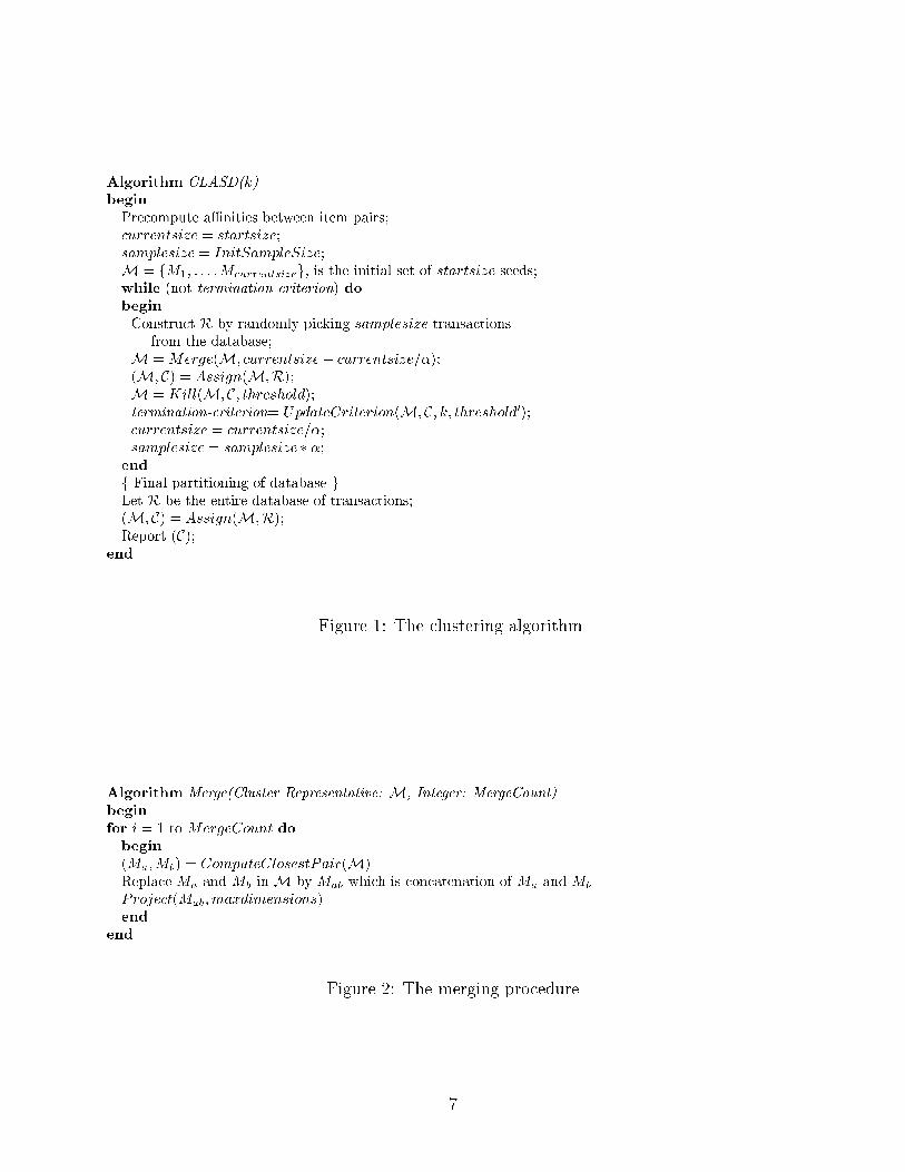
Algorithm CLASD(k)begin

Precompute a�nities between item pairs;currentsize = startsize;samplesize = InitSampleSize;M = fM1; : : : ;Mcurrentsizeg; is the initial set of startsize seeds;while (not termination-criterion) dobegin

Construct R by randomly picking samplesize transactionsfrom the database;

M = Merge(M; currentsize� currentsize=�);(M; C) = Assign(M;R);M = Kill(M; C; threshold);termination-criterion= UpdateCriterion(M; C; k; threshold0);currentsize = currentsize=�;samplesize = samplesize � �;

end

f Final partitioning of database gLet R be the entire database of transactions;(M; C) = Assign(M;R);Report (C);

end

Figure 1: The clustering algorithm

Algorithm Merge(Cluster Representative: M, Integer: MergeCount)begin

for i = 1 to MergeCount dobegin

(Ma;Mb) = ComputeClosestPair(M)Replace Ma and Mb in M by Mab which is concatenation of Ma and Mb

Project(Mab;maxdimensions)end

end

Figure 2: The merging procedure

7

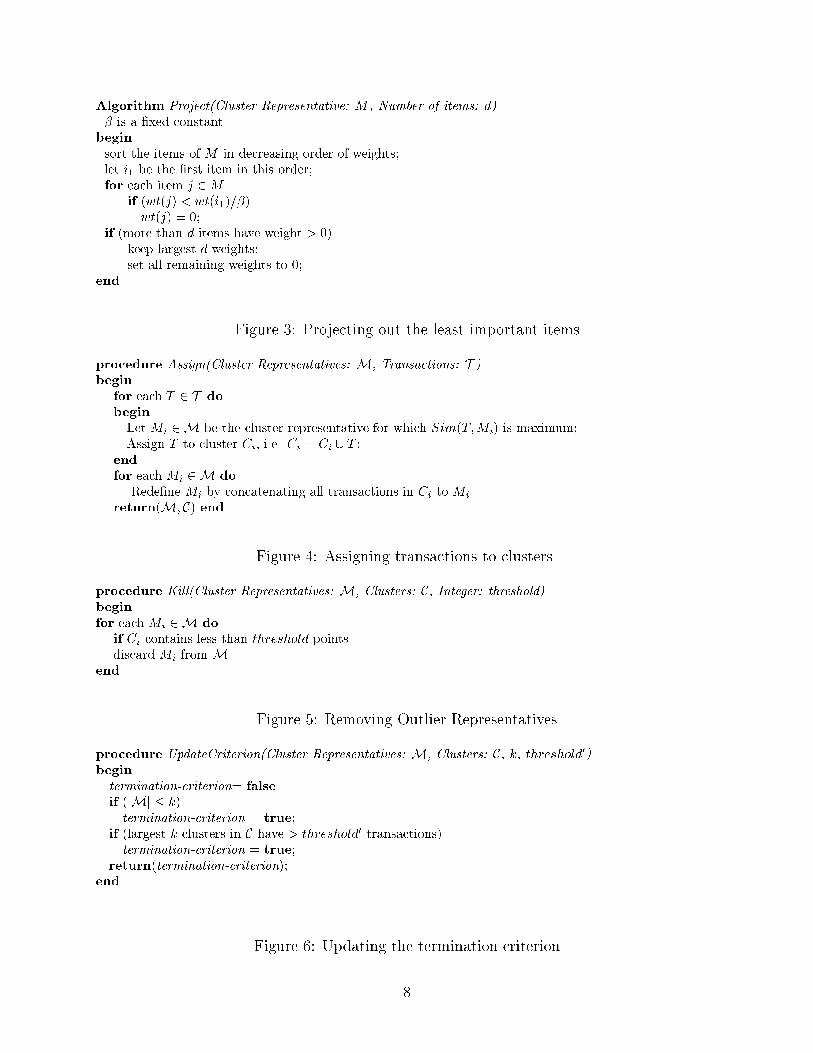
Algorithm Project(Cluster Representative: M , Number of items: d)� is a �xed constant

begin

sort the items of M in decreasing order of weights;let i1 be the �rst item in this order;for each item j 2M

if (wt(j) < wt(i1)=�)wt(j) = 0;

if (more than d items have weight > 0)keep largest d weights;set all remaining weights to 0;

end

Figure 3: Projecting out the least important items

procedure Assign(Cluster Representatives: M, Transactions: T )begin

for each T 2 T do

begin

Let Mi 2M be the cluster representative for which Sim(T;Mi) is maximum;Assign T to cluster Ci; i.e. Ci = Ci [ T ;

end

for each Mi 2M do

Rede�ne Mi by concatenating all transactions in Ci to Mi

return(M; C) end

Figure 4: Assigning transactions to clusters

procedure Kill(Cluster Representatives: M, Clusters: C, Integer: threshold)begin

for each Mi 2M do

if Ci contains less than threshold pointsdiscard Mi from M

end

Figure 5: Removing Outlier Representatives

procedure UpdateCriterion(Cluster Representatives: M, Clusters: C, k, threshold0)begin

termination-criterion= false

if (jMj � k)termination-criterion = true;

if (largest k clusters in C have > threshold0 transactions)termination-criterion = true;

return(termination-criterion);end

Figure 6: Updating the termination criterion

8

2.1 Implementing the merging operations e�ectively

Finally, we discuss the issue of how to merge the cluster representatives e�ectively. The idea

is to precompute some of the nearest neighbors of each representative at the beginning of

each Merge phase, and use these pre-computed neighbors in order to �nd the best merge.

After each merge operation between a meta-transactionM and its nearest neighbor (denoted

henceforth by nn[M ]) we need to delete M and nn[M ] from the nearest neighbor lists where

these representatives occured, and added the merged meta-transactionM 0 to the appropriate

nearest neighbor lists. If a list becomes empty, we recompute it from scratch. In some of

the implementations such as those discussed in ROCK [16], an ordered list of the distances

to all the other clusters is maintained for each cluster in a heap data structure. This results

in O(log n) time per update and O(n � log n) time for �nding the best merge. However, the

space complexity can be quadratic in terms of the initial number of representatives n.

Our implementation precomputed only a constant number of nearest neighbors for each

cluster representative. This implementation uses only linear space. Updating all lists takes

O(n) time per iteration, if no list becomes empty. This solution is also better than that of

always recomputing a single nearest neighbor (list size =1) for each representative, because

maintaining a larger list size reduces the likelihood of many lists becoming empty. Corre-

spondingly, the likelihood of having to spend O(n2) in one iteration is highly decreased. In

our experiments, we maintain the 5 closest neighbors of each representative. In general, if

at least one of the merged representatives M and nn[M ] appeared in the list of some other

representative N 2 M; then the resulting meta-transactionM 0 is one of the 5 nearest neigh-

bors of N: In all the experiments we performed, no list ever became empty, thus e�ectively

achieving both linear space and time for the maintenance of these lists.

2.2 Reporting item correlations

As discussed in Figure 1, the transactions are assigned to each cluster representative in a

�nal pass over the database. For an integrated application in which the correlations are

reported as an output of the clustering algorithm, the support counting can be parallelized

with this assignment process in this �nal pass. While assigning a transaction T to a cluster

representative M; we also update the information on the support supC(fi; jg) of each 2-item

pair fi; jg 2 T with respect to the corresponding cluster C. At the end, we report all pairs

of items whose support is above a user speci�ed threshold s in at least one cluster.

9

3 Time and Space Complexity

As discussed above, CLASD has space requirements linear in n; because we maintain only a

constant number of neighbors for each cluster. We also need to store the a�nity A(i; j) for

each pair of items (i; j) 2 U � U: Let D = jU j denote the total number of items in the data.

Then, the overall space required by CLASD is O(n+D2) = O(pN +D2):

Let Q� be the time required to calculate the similarity function. Thr running time may be

computing by summing the times required for the merge and assignment operations. The

nearest neighbor lists need to be initialized for each of the log�(n=k) sequences of Merge

operations. This requires O(n2 � Q� � log�(n=k)) time. Let nr denote the total number of

recomputations of nearest neighbor lists over all merges in the entire algorithm. This requires

n � nr � Q� time. Determining the optimum pair to be merged during each iteration takes

O(n) time. Each assignment procedure requires O(n � InitSampleSize �Q�) time (note that

the size of the random sample increases by the same factor by which the number of clusters

decreases). The last pass over the data which assigns the entire data set rather than a random

sample requires N � k �Q� time. Summing up everything, we obtain an overall running time

of O((n2 � Q� log�(n=k) + n � nr � Q� + n � InitSampleSize � log�(n=k)) � Q� + N � k � Q�) =

O((N �Q� log�(n=k) +pN � nr �Q� +

pN � InitSampleSize � log�(

pN=k)) �Q� +N � k �Q�):

Choosing di�erent values for InitSampleSize allows us a tradeo� between the accuracy and

running time of the method. As discussed earlier, the value of nr turned out to be small in

our runs, and did not contribute signi�cantly. Finally, to report the item correlations, we

spend O(D2 � k) time.

Number of disk accesses We access the entire data set at most thrice. During the

�rst access, we compute the a�nity matrix A, choose the random sample M of the initial

seeds, and also choose all independent random samples R (of appropriate sizes) that will be

used during various iterations to re�ne the clustering. The information on how many such

samples we need, and what their sizes are, can be easily computed if we know n; k; � and

InitSampleSize: Each random sample is stored in a separate �le. Since the sizes of these

random samples are in geometrically increasing order, and the largest random sample is at

most 1=� times the full database size, accessing these �les requires the equivalent of at most

one pass over the data for � � 2. The last pass over the data is used for the �nal assignment

of all transactions to cluster representatives.

10

4 Empirical Results

The simulations were performed on a 200-MHz IBM RS/6000 computer with 256MB of

memory, running AIX 4.3. The data was stored on a 4:5GB SCSI drive. We report results

obtained for both real and synthetic data. In all cases, we are interested in evaluating the

extent to which our segmentation method helps us discover new correlation among items, as

well as the scalability of our algorithm. We �rst explain our data generation technique and

then report on our experiments.

We have also implemented the ROCK algorithm (see [16]) and tested it both on the synthetic

and real data sets. In this method, the distance between two transactions is proportional to

the number of common neighbors of the transactions, where two transactions T1 and T2 are

neighbors if jT1\T2jjT1[T2j

� �: The number of clusters k and the value � are the main parameters

of the method.

4.1 Synthetic data generation

The synthetic data sets were generated using a method similar to that discussed in Agrawal

et. al. [4]. Generating the data sets was a two stage process:

(1) Generating maximal potentially large itemsets: The �rst step was to generate

L = 2000 maximal \potentially large itemsets". These potentially large itemsets cap-

ture the consumer tendencies of buying certain items together. We �rst picked the size

of a maximal potentially large itemset as a random variable from a poisson distribution

with mean �L. Each successive itemset was generated by picking half of its items from

the current itemset, and generating the other half randomly. This method ensures that

large itemsets often have common items. Each itemset I has a weight wI associated

with it, which is chosen from an exponential distribution with unit mean.

(2) Generating the transaction data: The large itemsets were then used in order to

generate the transaction data. First, the size ST of a transaction was chosen as a

poisson random variable with mean �T . Each transaction was generated by assigning

maximal potentially large itemsets to it in succession. The itemset to be assigned to a

transaction was chosen by rolling an L sided weighted die depending upon the weight

wI assigned to the corresponding itemset I. If an itemset did not �t exactly, it was

assigned to the current transaction half the time, and moved to the next transaction

the rest of the time. In order to capture the fact that customers may not often buy all

the items in a potentially large itemset together, we added some noise to the process

11

by corrupting some of the added itemsets. For each itemset I, we decide a noise level

nI 2 (0; 1). We generated a geometric random variable G with parameter nI . While

adding a potentially large itemset to a transaction, we dropped minfG; jIjg random

items from the transaction. The noise level nI for each itemset I was chosen from a

normal distribution with mean 0.5 and variance 0.1.

We shall also brie y describe the symbols that we have used in order to annotate the data.

The three primary factors which vary are the average transaction size �T , the size of an aver-

age maximal potentially large itemset �L, and the number of transactions being considered.

A data set having �T = 10, �L = 4, and 100K transactions is denoted by T10.I4.D100K.

The overall dimensionality of the generated data (i.e. the total number of items) was always

set to 1000.

4.2 Synthetic data results

For the remainder of this section, we will denote by AI(s) (aggregate itemsets) the set of

2-item-sets whose support relative to the aggregate database is at least s. We will also denote

by CI(s) (cluster partitioned itemsets) the set of 2-item-sets that have support s or more

relative to at least one of the clusters C generated by the CLASD algorithm (i.e., for any

pair of items (i; j) 2 CI(s); there exists a cluster Ck 2 C so that the support of (i; j) in

Ck is at least s). We shall denote the cardinality of the above sets by AI(s) and CI(s)

respectively. It is easy to see that AI(s) � CI(s) because any itemset which satis�es the

minimum support requirement with respect to the entire database must also satisfy it with

respect to at least one of the partitions. It follows that AI(s) � CI(s).

In order to evaluate the insight that we gain on item correlations from using our clustering

method, we have to consider the following issues.

1. The 2-item-sets in CI(s) are required to have smaller support, relative to the entire

data set, than the ones inAI(s); since jCij � N for any cluster Ci 2 C: Thus, we shouldcompare our output not only with AI(s); but also with AI(s0); for values s0 < s.

2. As mentioned above, AI(s) � CI(s): Thus, our method always discovers more corre-

lations among pairs of items, due to the relaxed support requirements. However, we

want to estimate how discriminative the process of �nding these correlations is. In

other words, we want to know how much we gain from our clustering method, versus

a random assignment of transactions into k groups.

12

1.5 2 2.5 3 3.5

x 10−3

0

0.5

1

1.5

2

2.5

3

3.5

4x 10

5

Support s

Num

ber

of 2

−ite

m−

sets

Aggregate Data Itemsets: AI(s/k) Cluster Partition Itemsets: CI(s) Aggregate Data Itemsets: AI(s)

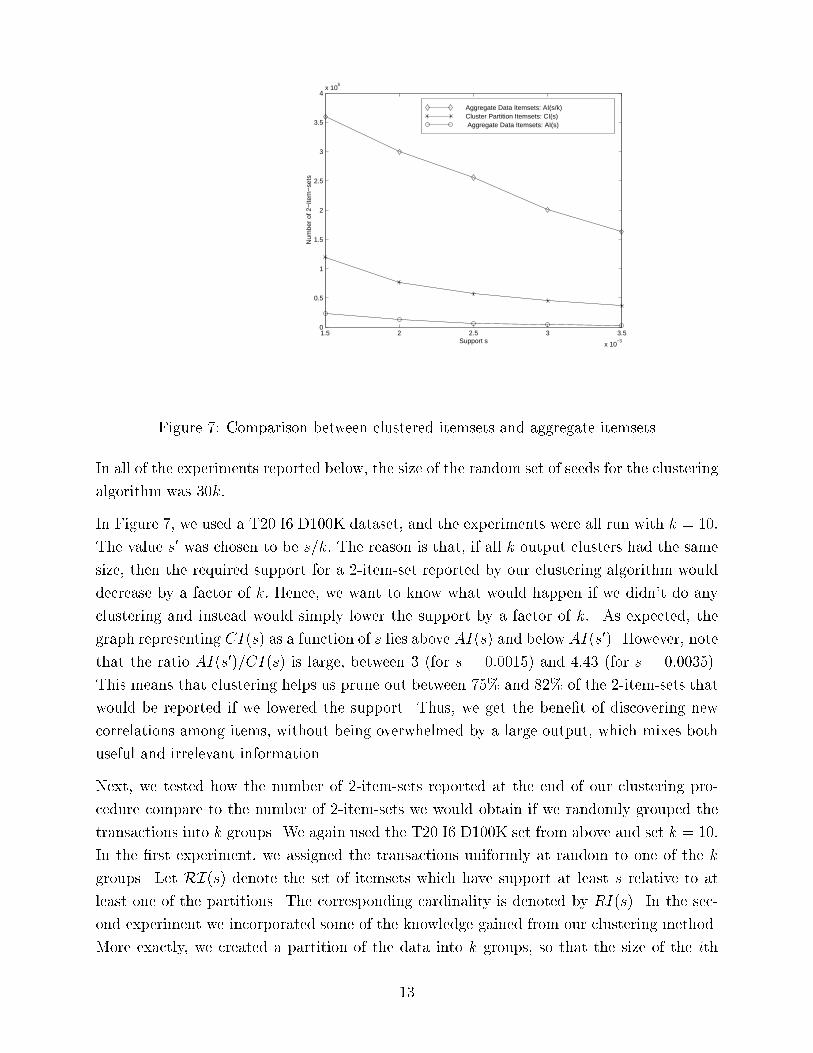
Figure 7: Comparison between clustered itemsets and aggregate itemsets

In all of the experiments reported below, the size of the random set of seeds for the clustering

algorithm was 30k:

In Figure 7, we used a T20.I6.D100K dataset, and the experiments were all run with k = 10:

The value s0 was chosen to be s=k: The reason is that, if all k output clusters had the same

size, then the required support for a 2-item-set reported by our clustering algorithm would

decrease by a factor of k: Hence, we want to know what would happen if we didn't do any

clustering and instead would simply lower the support by a factor of k:. As expected, the

graph representing CI(s) as a function of s lies above AI(s) and below AI(s0). However, note

that the ratio AI(s0)=CI(s) is large, between 3 (for s = 0:0015) and 4:43 (for s = 0:0035).

This means that clustering helps us prune out between 75% and 82% of the 2-item-sets that

would be reported if we lowered the support. Thus, we get the bene�t of discovering new

correlations among items, without being overwhelmed by a large output, which mixes both

useful and irrelevant information.

Next, we tested how the number of 2-item-sets reported at the end of our clustering pro-

cedure compare to the number of 2-item-sets we would obtain if we randomly grouped the

transactions into k groups. We again used the T20.I6.D100K set from above and set k = 10:

In the �rst experiment, we assigned the transactions uniformly at random to one of the k

groups. Let RI(s) denote the set of itemsets which have support at least s relative to at

least one of the partitions. The corresponding cardinality is denoted by RI(s). In the sec-

ond experiment we incorporated some of the knowledge gained from our clustering method.

More exactly, we created a partition of the data into k groups, so that the size of the ith

13

1.5 2 2.5 3 3.5

x 10−3

0

2

4

6

8

10

12x 10

4

Support s

Num

ber

of 2

−ite

m−

sets

Cluster Partition Itemsets CI(s) Clustersize Random Partition Itemsets RI"(s) Equal Random Partition Itemsets RI(s)

Figure 8: Comparison between Clustering and Random Partitions

group is equal to the size of the ith cluster obtained by our algorithm, and the transac-

tions are randomly assigned to the groups (subject to the size condition) The corresponding

set is denoted by RI"(s). The results are shown in Figure 8. Since RI(s) � RI"(s) for

all values of s considered, we restrict our attention to RI"(s): We used the same dataset

as above, and k = 10: Note that CI(s)=RI"(s) varies between 2:7 (for s = 0:0015) and

4:95 (for s = 0:0035), which shows that our clustering method signi�cantly outperforms an

indiscriminate grouping of the data.

Finally, in Figure 9, we show how the number of clusters k in uences the number of 2-item-

sets we report, for the T20.I6.D100K set used before. Again, we compare both with AI(s)

(which is constant, in this case) and with AI(s0); where s0 = s=k. We use s = 0:0025: The

fact that CI(s) increases with k corresponds to the intuition that grouping into more clusters

implies lowering the support requirement.

The examples above illustrate that the itemsets found are very di�erent depending upon

whether we use localized analysis or aggregate analysis. From the perspective of a target

marketing or customer segmentation application, such correlations may have much greater

value than those obtained by analysis of the full data set.

The next two �gures illustrate how our method scales with the number of clusters k and

the size of the dataset N: In Figure 10, we �x N = 100000; while in Figure 11 we �x

k = 10: We separately graph the running time spent on �nding the cluster representatives

before performing the �nal partitioning procedure of the entire database into clusters using

14

6 7 8 9 10 11 120

0.5

1

1.5

2

2.5

3x 10

5

Number of clusters k

Num

ber

of 2

−ite

m−

sets

Aggregate Data Itemsets AI(s/k)Cluster Parition Itemsets CI(s)Aggregate Data Itemsets AI(s)

Figure 9: Comparison between clustered itemsets and aggregate itemsets

these representatives. Clearly, the running time for the �nal phase requires O(k �N) distance

computations; something which we cannot hope to easily outperform for any algorithmwhich

attempts to put N points into k clusters. If we can show that the running time for the entire

algorithm before this phase is small compared to this, then our running times are close to

optimal. Our analysis of the previous section shows that this time is quadratic in the size

of the random sample, which in turn is linear in k: On the other hand, the time spent on

the last step of the method to assign all transactions to their respective clusters is linear in

both k and N: As can be noted from Figures 10 and 11, the last step clearly dominates the

computation, and so overall the method scales linearly with k and N:

Comparison with ROCK We ran ROCK on the synthetically generated T20.I6.D100K

dataset used above, setting k = 10 and � = 0:1 (recall that � is the minimum overlap

required between two neighbor clusters). We wanted to report all 2-item-sets with support

s � 0:0025 in at least one of the generated clusters. ROCK obtained a clustering in which one

big cluster contained 86% of the transactions, a second cluster had 3% of the transactions,

and the sizes of the remaining clusters varied around 1% of the data. This result is not

surprising if we take into account the fact that the overall dimensionality of the data space

is 1000; while the average number of items in a transaction is 20: Thus, the likelihood of two

transactions sharing a signi�cant percentage of items is low. This means that the number

of pairs of neighbors in the database is quite small, which in turn implies that the number

of links between two transactions is even smaller (recall that the number of links between

15

6 7 8 9 10 11 120

100

200

300

400

500

600

700

800

Number of clusters k

Run

ning

tim

e in

sec

onds

Total time Finding Cluster Representatives

Figure 10: Running Time Scalability (Number of Clusters)

1 2 3 4 5 6 7 8 9 10

x 105

0

1000

2000

3000

4000

5000

6000

Number of transactions N

Run

ning

tim

e in

sec

onds

Total time Finding Cluster Representatives

Figure 11: Running Time Scalability (Number of Transactions)

16

Output Clusters Edible Poisonous Output Clusters Edible Poisonous

1 2263 56 11 354 7

2 31 1776 12 192 3

3 0 269 13 233 0

4 0 290 14 0 151

5 0 180 15 8 263

6 593 0 16 0 124

7 0 146 17 0 103

8 0 133 18 0 218

9 150 124 19 232 0

10 2 68 20 150 5

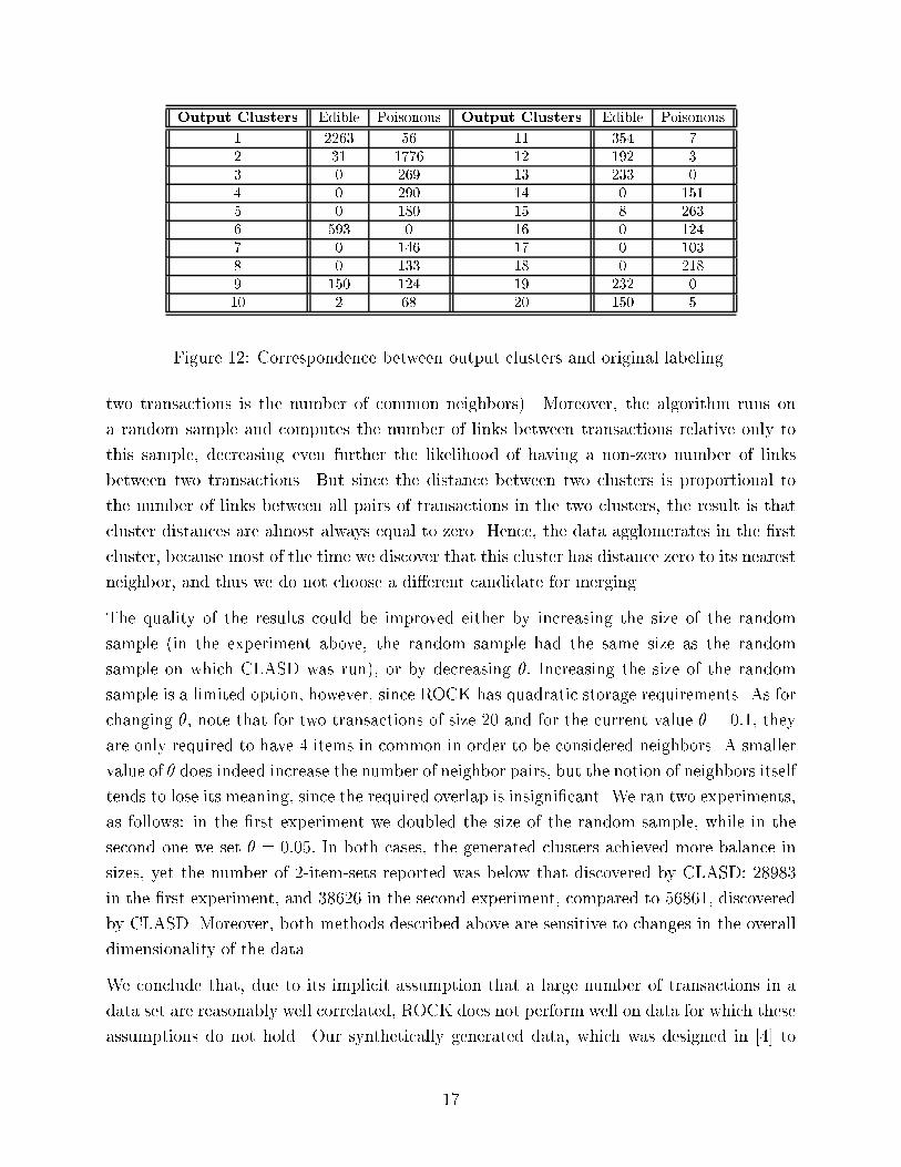
Figure 12: Correspondence between output clusters and original labeling

two transactions is the number of common neighbors). Moreover, the algorithm runs on

a random sample and computes the number of links between transactions relative only to

this sample, decreasing even further the likelihood of having a non-zero number of links

between two transactions. But since the distance between two clusters is proportional to

the number of links between all pairs of transactions in the two clusters, the result is that

cluster distances are almost always equal to zero. Hence, the data agglomerates in the �rst

cluster, because most of the time we discover that this cluster has distance zero to its nearest

neighbor, and thus we do not choose a di�erent candidate for merging.

The quality of the results could be improved either by increasing the size of the random

sample (in the experiment above, the random sample had the same size as the random

sample on which CLASD was run), or by decreasing �: Increasing the size of the random

sample is a limited option, however, since ROCK has quadratic storage requirements. As for

changing �; note that for two transactions of size 20 and for the current value � = 0:1; they

are only required to have 4 items in common in order to be considered neighbors. A smaller

value of � does indeed increase the number of neighbor pairs, but the notion of neighbors itself

tends to lose its meaning, since the required overlap is insigni�cant. We ran two experiments,

as follows: in the �rst experiment we doubled the size of the random sample, while in the

second one we set � = 0:05: In both cases, the generated clusters achieved more balance in

sizes, yet the number of 2-item-sets reported was below that discovered by CLASD: 28983

in the �rst experiment, and 38626 in the second experiment, compared to 56861, discovered

by CLASD. Moreover, both methods described above are sensitive to changes in the overall

dimensionality of the data.

We conclude that, due to its implicit assumption that a large number of transactions in a

data set are reasonably well correlated, ROCK does not perform well on data for which these

assumptions do not hold. Our synthetically generated data, which was designed in [4] to

17

resemble the real market basket data, is an example of such input.

We tested both CLASD and ROCK on the mushroom and adult data sets from the ML

Repository1.

4.3 The mushroom data set

The mushroom data set contained a total of 8124 instances. Each entry has 22 categorical

attributes (e.g. cap-shape, odor etc.), and is labeled either \edible" or \poisonous". We

transformed each such record into a transaction in the same manner used by [16]: for each

attribute A and each value v in the domain of A; we introduce the item A:v: A record R is

transformed into a transaction T so that T contains item A:v if and only if R has value v

for attribute A:

We ran ROCK with the parameters indicated in [16], i.e. k = 20 and � = 0:8; and were able

to con�rm the results reported by the authors on this data set, with minor di�erences. The

number of 2-item-sets discovered after clustering was 1897, at support level s = 0:1.

To test CLASD on this data set, we must take into account the fact that if attribute A

has values in the domain fv; wg; then items A:v and A:w will never appear in the same

transaction. We want to make a distinction between this situation, and the situation when

two items do not appear together in any transaction in the database, yet they do not ex-

clude one another. Hence, we de�ne a negative a�nity for every pair of items (A:v; A:w)

as above. We present the results in Figure 12. With the exception of cluster number 9,

which draws about half of its records from each of the two classes of mushrooms, the other

clusters clearly belong to either the \edible" or \poisonous" categories, although some have

a small percentage of records from the other category (e.g., clusters 1 and 2). We believe

that the latter is due to the fact that our distance function is a heuristic designed to max-

imize the number of 2-itemsets with enough support in each cluster. This may induce the

\absorption" of some poisonous mushrooms into a group of edible mushrooms, for example,

if this increases the support of many pairs of items. The number of 2-item-sets discovered

was 2155, for support level s = 0:1; which is superior to that reported by ROCK. We also

computed the number of 2-item-sets using the original labels to group the data into two

clusters (\edible" and \poisonous"), and found 1123 2-itemsets with enough support relative

to at least one such cluster. Hence, our segmentation method proves useful for discovering

interesting correlations between items even when a previous labeling exists.

Aside from this, we also found some interesting correlations which cannot be found by only

1http : ==www:ics:uci:edu=~mlearn=MLRepository:html

18

looking at the labels. For the support level s = 0:1 = 10%; we could not �nd a correlation

between convex caps and pink gills, since this pair of characteristics appears together in

750 species of mushrooms, or 9:2% of the data. Such a correlation between this pair is

useful enough, and it should be recognized and reported. We also could not discover this c

orrelation by treating the original labels as two clusters, because there are 406 edible species

with these two characteristics, or 9:6% of the edible entries, and 344 poisonous species, or

8:7% of all poisonous entries. However, our technique creates a structured segmentation in

which the correlation is found.

4.4 The adult data set

We also tested the algorithm for the adult data set in the UCI machine learning respository.

The data set was extracted from the 1994 census data and contained information about

demographic data about people. This data set had a total of 32562 instances. Among these

instances, 8 were categorical valued. We �rst transformed the categorical attributes to bi-

nary data. This resulted in a total of 99 binary attributes. One observation on this data set

was that there were a signi�cant number of attributes in the data which corresponded to a

particular value. For example, most records were from the United States, one of the �elds

was "Private" a large fraction of the time, and the data largely consisted of whites. There

is not much information in these particular attributes, but the ROCK algorithm often built

linkages based on these attributes and resulted in random assignments of points to clusters.

We applied the CLASD algorithm to the data set with k = 100, and found several interest-

ing 2-itemsets in the local clusters which could not be discovered in the aggregate data set.

For example, we found a few clusters which contained a disproportionate number of females

who were either "Unmarried" or in the status \Not-in-family". (In each of these clusters, the

support of (Female, Unmarried) and (Female, Not-in-family) was above 30%.) This behavior

was not re ected in any of the clusters which had a disproportionately high number of men.

For the case of men, the largest share tended to be \husbands". Thus, there was some asym-

metry between men and women in terms of the localized 2-itemsets which were discovered.

This asymmetry may be a function of how the data was picked from the census; speci�cally

the data corresponds to behavior of employed people. Our analysis indicates that in some

segments of the population, there are large fractions of employed women who are unmarried

or not in families. The correlation cannot be discovered by the aggregate support model,

since the required support level of 8:1% (which is designed to catch both the 2-itemsets)

is so low that it results in an extraodinarily high number of meaningless 2-itemsets along

with the useful 2-itemsets. Such meaningless 2-itemsets create a di�culty in distinguishing

the useful information in the data from noise. Another interesting observation was a clus-

19

ter in which we found the following 2-itemsets: (Craft-Repair, Male), and (Craft-Repair,

HS-grad). This tended to expose a segment of the data containing males with relatively

limited education who were involved in the job of craft-repair. Similar segmented 2-itemsets

corresponding to males with limited educational level were observed for the professions of

Transport-Moving and Farming-Fishing. Another interesting 2-itemset which we discovered

from one of the segments of the data set was (Doctorate, Prof-specialty). This probably

corresponded to a segment of the population which was highly educated and was involved

in academic activities such as professorships. We also discovered a small cluster which had

the 2-itemset (Amer-Indian-Eskimo, HS-Grad) with a support of 50%. Also, most entries

in this segment corresponded to American-Indian Eskimos, and tended to have educational

level which ranged from 9th grade to high school graduate. This exposes an interesting

demographic segment of the people which shows a particular kind of association. Note that

the absolute support of this association relative to the entire data set is extremely low, since

there are only 311 instances of American Indian Eskimos in the data base of 32562 instances

(less than 1%). The 2-itemsets in most of the above cases had a support which was too low

to be discovered by aggregate analysis, but turned out to be quite dominant and interesting

for particular segments of the population.

5 Conclusions and Summary

In this paper we discussed a new technique for clustering market basket data. This technique

may be used for �nding signi�cant localized correlations in the data which cannot be found

from the aggregate data. Our empirical results illustrated that our algorithm was able to

�nd a signi�cant percentage of itemsets beyond a random partition of the transactions. Such

information may prove to be very useful for target marketing applications. Our algorithm can

also be generalized easily to categorical data. We showed that in such cases, the algorithm

performs better than ROCK in �nding localized associations.

References

[1] C. C. Aggarwal, P. S. Yu. \Finding Generalized Projected Clusters in High Dimensional

Spaces" Proceedings of the ACM SIGMOD Conference, 2000.

[2] C. C. Aggarwal, P. S. Yu. \A new framework for itemset generation." Proceedings of the

ACM PODS Conference, 1998.

20

[3] R. Agrawal, T. Imielinski, A. Swami. \Mining association rules between sets of items in

very large databases." Proceedings of the ACM SIGMOD Conference on Management of

data, pages 207-216, 1993.

[4] R. Agrawal, R. Srikant. Fast Algorithms for Mining Association Rules in Large

Databases. Proceedings of the 20th International Conference on Very Large Data Bases,

pages 478-499, September 1994.

[5] R. Agrawal, J. Gehrke, D. Gunopulos, P. Raghavan. \Automatic Subspace Clustering of

High Dimensional Data for Data Mining Applications", Proceedings of the ACM SIG-

MOD Conference, 1998.

[6] M. Ankerst, M. M. Breunig, H.-P. Kriegel, J. Sander. \OPTICS: Ordering Points To

Identify the Clustering Structure." Proceedings of the ACM SIGMOD Conference, 1999.

[7] S. Chakrabarti, S. Sarawagi, B. Dom. \Mining surprising patterns using temporal de-

scription length." Proceedings of the International Conference on Very Large Databases,

August 1999.

[8] C. Silverstein, R. Motwani, S. Brin. \Beyond Market Baskets: Generalizing association

rules to correlations." Proceedings of the ACM SIGMOD Conference, 1997.

[9] M. Ester, H.-P. Kriegel, J. Sander, M. Wimmer, X. Xu. \Incremental Clustering for

Mining in a Data Warehousing Environment." Proccedings of the Very Large Databases

Conference, 1998.

[10] M. Ester, H.-P. Kriegel, X. Xu. \A Database Interface for Clustering in Large Spatial

Databases", Proceedings of the Knowledge Discovery and Data Mining Conference, 1995.

[11] M. Ester, H.-P. Kriegel, J. Sander, X. Xu. \A Density Based Algorithm for Discovering

Clusters in Large Spatial Databases with Noise", Proceedings of the Knowledge Discovery

in Databases and Data Mining Conference, 1995.

[12] U. M. Fayyad, G. Piatetsky-Shapiro, P. Smyth. \From Data Mining to Knowledge

Discovery: An Overview." Advances in Knowledge Discovery and Data Mining. U. M.

Fayyad et. al. (Eds.) AAAI/MIT Press.

[13] V. Ganti, J Gehrke, R. Ramakrishnan. \CACTUS: Clustering Categorical Data Using

Summaries", Proceedings of the ACM SIGKDD Conference, 1999.

[14] D. Gibson, J. Kleinberg, P. Raghavan. \Clustering Categorical Data: An Approach

Based on Dynamical Systems", Proceedings of the VLDB Conference, 1998.

21

[15] S. Guha, R. Rastogi, K. Shim. \CURE: An E�cient Clustering Algorithm for Large

Databases", Proceedings of the ACM SIGMOD Conference, 1998.

[16] S. Guha, R. Rastogi, K. Shim. \ROCK: a robust clustering algorithm for categorical

attributes", Proceedings of the International Conference on Data Engineering, 1999.

[17] E.-H. Han, G. Karypis, V. Kumar, B. Mobasher. \Clustering based on association rule

hypergraphs", Proceedings of the ACM SIGMOD Workshop, 1997.

[18] H. V. Jagadish, L. V. S. Lakshmanan, D. Srivastava. \Snakes and Sandwiches: Op-

timal Clustering Strategies for a Data Warehouse", Proceedings of the ACM SIGMOD

Conference, 1999.

[19] A. Jain, R. Dubes. Algorithms for Clustering Data, Prentice Hall, New Jersey, 1998.

[20] L. Kaufman, P. Rousseuw. \Finding Groups in Data- An Introduction to Cluster Anal-

ysis." Wiley Series in Probability and Mathematical Sciences, 1990.

[21] M. Klementtinen, H. Mannila P. Ronkainen, H. Toivonen, A. I. Verkamo \Finding

Interesting Rules from Large Sets of discovered association rules." Third International

Conference on Information and Knowledge Management, pages 401-407, 1994.

[22] R. Ng, J. Han. \E�cient and E�ective Clustering Methods for Spatial Data Mining",

Proceedings of the Very Large Data Bases Conference, 1994.

[23] G. Salton, M. J. McGill. Introduction to Modern Information Retrieval. Mc Graw Hill,

New York.

[24] K. Chakrabarti, S. Mehrotra. Local Dimensionality Reduction: A New Approach to

Indexing High Dimensional Spaces. Proceedings of the VLDB Conference, 2000.

[25] X. Xu, M. Ester, H.-P. Kriegel, J. Sander. \A Distribution-Based Clustering Algorithm

for Mining in Large Spatial Databases", Proceedings of the ICDE Conference, 1998.

[26] M. Zait, H. Messatfa. \A Comparative Study of Clustering Methods", FGCS Journal,

Special Issue on Data Mining, 1997.

[27] T. Zhang, R. Ramakrishnan, M. Livny. \BIRCH: An E�cient Data Clustering Method

for Very Large Databases", Proceedings of the ACM SIGMOD Conference, 1996.

22