Finding Approximate Areas Under Curves

The Trapezium Rule

y0 y1 y2 y3 y4 y5

This curve has a complicated equation so instead of integrating split the area up into a number of trapeziums each of width h and find the area of each.

The y coordinates are given by y0, y1, y2, y3 etc

Proving the Formula

• Area of trapezium 1 = • Area of Trapezium 2 = • Area of Trapezium 3 = • Area of Trapezium 4 =• Area of Trapezium 5 =

y0 y1 y2 y3 y4 y5

h= strip width

= interval width

h

1/2(y0 + y1) x h1/2(y1 + y2) x h1/2(y2 + y3) x h1/2(y3 + y4) x h1/2(y4 + y5) x h

Proving the Formula

• Area = 1/2h(y0 + y1+ y1+ y2 + y2…yn)

• = 1/2h(y0 + 2y1+ 2y2 + 2y3…yn)

• = 1/2h(y0 + 2(y1 + y2 + y3…) + yn)

y0 y1 y2 y3 y4 y5

h

Simpsons Rule

Who was William Simpson?

Simpson was born in Market Bosworth, Leicestershire. The son of a weaver, Simpson taught himself mathematics, then turned to astrology after seeing a solar eclipse. He also dabbled in witchcraft and caused fits in a girl after 'raising a devil' from her. After this incident, he and his wife had to flee to London.

From 1743, he taught mathematics at the Royal Military Academy, Woolwich.Apparently, the method that became known as Simpson's rule was well known and used earlier by Bonaventura Cavalieri (a student of Galileo) in 1639. It was later rediscovered by James Gregory (who Simpson succeeded as Professor of Mathematics at the University of St Andrews) but was only attributed to Simpson.

In 1758, Simpson was elected a foreign member of the Royal Swedish Academy of Sciences.

Simpson's rule is a staple of scientific data analysis and engineering. It is widely used, for example, by Naval architects to calculate the capacity of a ship or lifeboat.

Simpsons RuleThis approximates the area under the curve using a quadratic curve to join the tops of each y value rather than a straight line as in the trapezium rule

y0 y1 y2 y3 y4 y5

2xey

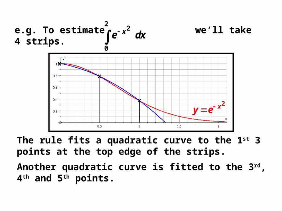
e.g. To estimate we’ll take 4 strips. 2

0

2dxe x

The rule fits a quadratic curve to the 1st 3 points at the top edge of the strips.

x

x

x

2xey

x

x

x

e.g. To estimate we’ll take 4 strips. 2

0

2dxe x

The rule fits a quadratic curve to the 1st 3 points at the top edge of the strips.

Another quadratic curve is fitted to the 3rd, 4th and 5th points.

2xey x

e.g. To estimate we’ll take 4 strips. 2

0

2dxe x

The rule fits a quadratic curve to the 1st 3 points at the top edge of the strips.

Another quadratic curve is fitted to the 3rd, 4th and 5th points.

xx

2xey x

x

x

e.g. To estimate we’ll take 4 strips. 2

0

2dxe x

The rule fits a quadratic curve to the 1st 3 points at the top edge of the strips.

Another quadratic curve is fitted to the 3rd, 4th and 5th points.

Consider three points which have coordinates(-h, y0), (0, y1), (h, y2).The tops of each red bar are joined by a quadratic curve(parabola) rather than straight lines as in the trapezium ruleThe parabola has the equation :

-1

1

2

3

4

5

6

7

8

-1 1 20X->

|̂Y

-h h0

y0

y1y2

(-h, y0),

(0, y1)

(h, y2)

y = ax2 + bx + c

The object is to find the area of the 2 strips shown using the y coordinates and then extend the idea to the next 2 strips.

-1

1

2

3

4

5

6

7

8

-1 1 20X->

|̂Y

-h h0

y0

y1y2

y = ax2 + bx + c.

-1

1

2

3

4

5

6

7

8

-1 1 20X->

|̂Y

-h h0

y0

y1y2

A=

 

  Now substitute in the boundaries i.e x=h and x=-h

y = ax2 + bx + c.

ydx

-1

1

2

3

4

5

6

7

8

-1 1 20X->

|̂Y

-h h0

y0

y1y2

 

  

  

y = ax2 + bx + c.

-1

1

2

3

4

5

6

7

8

-1 1 20X->

|̂Y

-h h0

y0

y1y2

    

A=    

      

y = ax2 + bx + c.

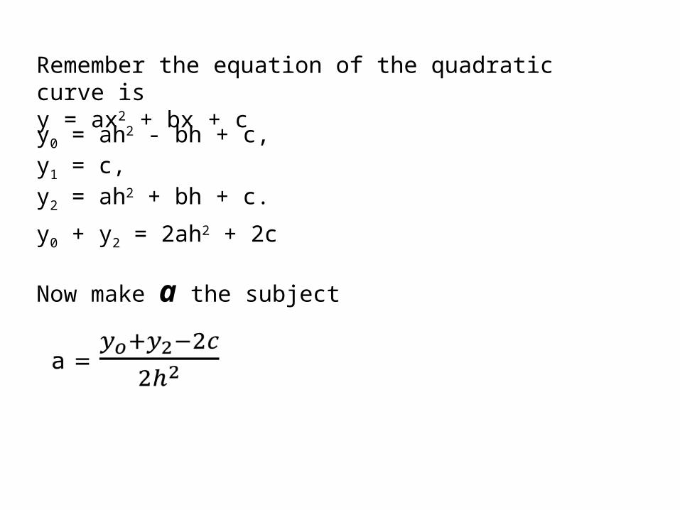
When we substitute the coordinates of the three points (-h, y0), (0, y1), (h, y2) into the equation for the parabola, we obtain the three equationsy0 = ah2 - bh + c,y1 = c,y2 = ah2 + bh + c.

Remember the equation of the quadratic curve is y = ax2 + bx + c

If we add the 1st and 3rd equation then we obtain

y0 + y2 = 2ah2 + 2c

Now make a the subject

y0 = ah2 - bh + c,y1 = c,y2 = ah2 + bh + c.

Remember the equation of the quadratic curve is y = ax2 + bx + c

y0 + y2 = 2ah2 + 2c

Now make a the subject

 

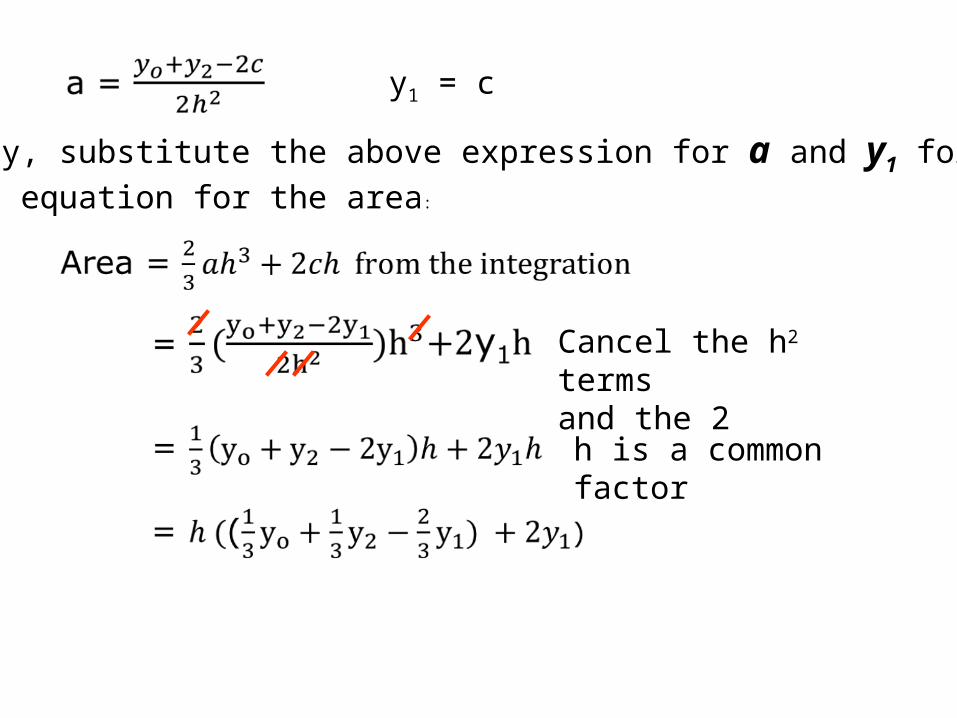
Finally, substitute the above expression for a and y1 for c

in the equation for the area:

 

 

  Cancel the h2 termsand the 2

 

y1 = c

h is a common factor

 

 

 

 

 

 

 

h is a common factor

 

 

 

h

  h

  h

h

  h h

 

The formula works providingThe number of y values is………….And the number of strips is ………..

ODDEVEN

h

h

1

021

1dx

x

e.g. (a) Use Simpson’s rule with 4 strips to estimate

giving your answer to 4 d.p.

Solution: (a) 43210 424

3yyyyy

hA

-1

1

-1 1 20X->

|̂Y

y0y2

y1

y4

y3

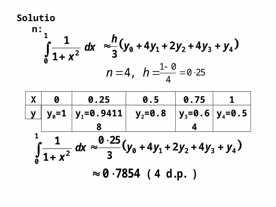
Solution:

4,n h

1

021

1dx

x 43210 4243

yyyyyh

) d.p. ( 478540

1

021

1dx

x 43210 424

3

250yyyyy

X 0 0.25 0.5 0.75 1y y0=1 y1=0.94118 y2=0.8 y3=0.64 y4=0.5

1 00 25

4

) d.p. ( 478540

1

021

1dx

x(a

)

(b) Use your calculator to check the answer using the integration button

Exercise

3

1

1dx

xusing Simpson’s

rule

with 2 strips, giving your answer to 4 d.p.

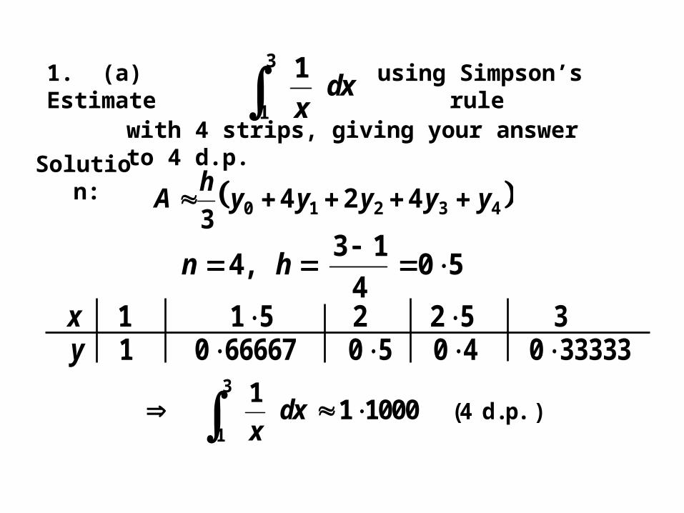
1. (a) Estimate

(b) Improve your answer using 4 strips

Solution:

using Simpson’s rule

with 2 strips, giving your answer to 4 d.p.

1. (a) Estimate3

1

1dx

x

-1

1

2

3

4

5

1 2 3 40X->

|̂Y

y0 y1 y2

210 yy4y3

hA

Solution:

using Simpson’s rule

with 2 strips, giving your answer to 4 d.p.

1. (a) Estimate3

1

1dx

x

2,n h

(4 d.p. )3

1

1dx 1 1111

x

X 1 2 3y y0=1 y1=0.5 y2=0.33333

3 11

2

43210 4243

yyyyyh

A Solutio

n:

using Simpson’s rule

with 4 strips, giving your answer to 4 d.p.

1. (a) Estimate3

1

1dx

x

504

13,4

hn

3522511 x33333040506666701 y

) d.p. 4(1000113

1 dx

x