Financial Stress and Equilibrium Dynamics in Money Markets · · 2015-10-15Financial Stress and...

Finance and Economics Discussion SeriesDivisions of Research & Statistics and Monetary Affairs

Federal Reserve Board, Washington, D.C.

Financial Stress and Equilibrium Dynamics in Money Markets

Emre Yoldas and Zeynep Senyuz

2015-091

Please cite this paper as:Yoldas, Emre, and Zeynep Senyuz (2015). “Financial Stress and Equilibrium Dynamics inMoney Markets,” Finance and Economics Discussion Series 2015-091. Washington: Boardof Governors of the Federal Reserve System, http://dx.doi.org/10.17016/FEDS.2015.091.

NOTE: Staff working papers in the Finance and Economics Discussion Series (FEDS) are preliminarymaterials circulated to stimulate discussion and critical comment. The analysis and conclusions set forthare those of the authors and do not indicate concurrence by other members of the research staff or theBoard of Governors. References in publications to the Finance and Economics Discussion Series (other thanacknowledgement) should be cleared with the author(s) to protect the tentative character of these papers.

Financial Stress and Equilibrium Dynamics in Money Markets∗

Emre Yoldas† Zeynep Senyuz‡

August 2015

Abstract

Interest rate spreads are widely-used indicators of funding pressures and market func-tioning in money markets. Using weekly data from 2002 to 2015, we analyze money marketdynamics in a long-run equilibrium framework where commonly-monitored spreads serve aserror correction terms. We find strong evidence for nonlinearities with respect to levels of thespreads. We provide point and interval estimates for spread thresholds that quantify fundingpressure points from a long-run perspective. Our results indicate significant asymmetry inthe adjustment toward long-run equilibrium. We show that economically and statisticallysignificant adjustments occur only following large shocks to risk premia. Additionally, wequantify shifts in interest rate volatilities in high spread regimes characterized by elevatedfunding stress as well as declining correlations between risky funding rates and relatively safebase rates in such environments.

Keywords: Money markets, Cointegration, Threshold models, GARCH, Constant conditionalcorrelation model.

JEL Classification: C32, E44, E52

∗We would like to thank Beth Klee, Karin Loch, seminar participants at the Federal Reserve Board and AmericanUniversity, participants of the Annual Symposium of the Society for Nonlinear Dynamics and Econometrics, andInternational Workshop on Financial Markets and Nonlinear Dynamics for useful comments. We thank FrancescaCavalli for preparing the data set. Special thanks to Bernd Schlusche and Selva Demiralp for their contributionsto an earlier version of this paper. The views expressed in this paper are solely the responsibility of the authorsand should not be interpreted as reflecting the views of the Board of Governors of the Federal Reserve System orof anyone else associated with the Federal Reserve System.†Federal Reserve Board, Division of Monetary Affairs. E-mail: [email protected]‡Federal Reserve Board, Division of Monetary Affairs. E-mail: [email protected]

mailto:[email protected]

mailto:[email protected]

1 Introduction

In money markets, a wide array of participants trade highly liquid, short-term, and low-risk debt.

Since banks and other financial institutions meet their marginal funding needs in money markets,

strains in these markets may impair the flow of credit to the entire economy, e.g. Ivashina et al.

(2015). The money market also plays a key role in monetary policy implementation. The Federal

Reserve typically relies on the strong comovement between its target rate, the federal funds rate,

and other short-term interest rates for effective transmission of its monetary policy.

Until the recent global financial crisis, money market rates were moving in tandem, with

generally stable and narrow spreads between them. However, at the onset of the crisis in the

summer of 2007, conditions in short-term funding markets changed considerably and persistent

spikes in key money market spreads emerged. The Federal Reserve responded to the crisis with a

variety of new facilities and unconventional tools, such as the Term Auction Facility, to provide

liquidity to the financial system. Following several cuts to its policy rate starting in mid-2007,

the Federal Reserve announced a target range of 0− 0.25% percent for the federal funds rate in

December 2008. The federal funds rate and the other overnight funding rates have been near

the zero-lower bound (ZLB) since then. In the aftermath of the crisis, abundant reserves in

the system, higher risk perception of market participants associated with wholesale funding, and

new regulations concerning the management of liquidity risk at large financial institutions have

defined the new money market environment.

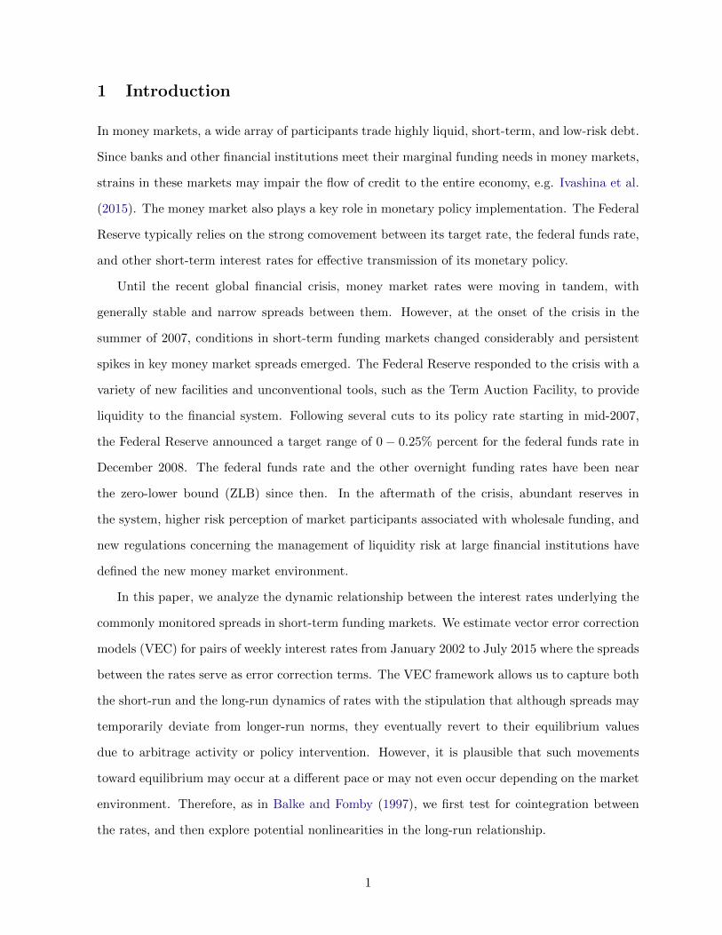
In this paper, we analyze the dynamic relationship between the interest rates underlying the

commonly monitored spreads in short-term funding markets. We estimate vector error correction

models (VEC) for pairs of weekly interest rates from January 2002 to July 2015 where the spreads

between the rates serve as error correction terms. The VEC framework allows us to capture both

the short-run and the long-run dynamics of rates with the stipulation that although spreads may

temporarily deviate from longer-run norms, they eventually revert to their equilibrium values

due to arbitrage activity or policy intervention. However, it is plausible that such movements

toward equilibrium may occur at a different pace or may not even occur depending on the market

environment. Therefore, as in Balke and Fomby (1997), we first test for cointegration between

the rates, and then explore potential nonlinearities in the long-run relationship.

1

We find strong evidence in favor of both cointegration and asymmetric dynamics in the rela-

tionship between the considered interest rates. Therefore, we estimate a nonlinear version of the

VEC model, the so-called threshold VEC model (TVEC), where different states of the market are

identified by the level of the spreads that serve as thresholds. This allows us to characterize the

discrete adjustment mechanism in the form of threshold cointegration where the cointegrating

relation may be muted in a certain range of the relevant spread, but becomes active once the sys-

tem is sufficiently far away from the equilibrium. We provide estimates and subsampling-based

confidence intervals for spread thresholds to quantify funding pressure points from a long-run

perspective and determine regimes characterized by different levels of funding stress. In addition,

we quantify abrupt shifts in volatilities of interest rates in high spread regimes associated with

elevated funding stress. We also show that correlations between risky and relatively safe base

rates decline considerably in such regimes.

Our results indicate significant asymmetries in the equilibrium adjustment mechanism, which

are masked in a conventional linear model. We find that economically and statistically significant

adjustment toward long-run equilibrium occurs following large shocks to risk premia. This result

is robust to differences arising from the use of spot and forward rates or the duration of the

underlying loans. However, adjustments in relatively low spread environments change with respect

to such characteristics. We also find that adjustments can take place through different rates

depending on the market segment. For example, in case of the relationship between an interbank

term funding rate and the expected policy rate, the adjustment occurs through the former,

while the secured rate plays a bigger role in bringing the system back to equilibrium in the

case of overnight rates. Our findings on adjustment dynamics are consistent with the combined

effects of policy intervention aimed at reducing risk spreads and market response to high levels of

compensation for risk. Our results also emphasize the additional information content of forward

spreads for risk monitoring as well as the effects of flight-to-quality flows on market dynamics

during times of stress.

Our paper is related to two important strands of the literature. First, several studies develop

composite indexes that attempt to measure stress in financial markets, see for example, Carlson

et al. (2011), Hakkio and Keeton (2009), and Oet et al. (2011) among others. These studies

rely on various sets of spreads between rates on risky and riskless assets, liquidity measures,

2

credit flows, as well as implied and realized volatilities to construct composite indicators for

measurement of financial stress. Carpenter et al. (2014) develops an index for the money market

in a similar framework. In contrast, we analyze different market segments separately in a long-

run cointegration framework. This allows us to detect stress that may appear in one part of the

market while not being reflected in the funding conditions prevailing in the rest of the market.

Moreover, our flexible modeling approach allows us to characterize the evolution of mean, variance

and correlation dynamics in different market segments in addition to providing estimates of

stress thresholds for market monitoring. Second, our study is also related to the literature that

focuses on state dependent comovement in asset prices (see for example Vayanos (2004), He

and Krishnamurthy (2012), and Brunnermeier and Sannikov (2014) for theoretical treatments).

In this context, we show that the error correction mechanism exhibits asymmetry in different

regimes of the money market determined by the risk premia and that correlations between rates

are highly state dependent.

The remainder of the paper proceeds as follows: Section 2 describes the data and provides

some background information about the key interest rates and the corresponding spreads. Section

3 introduces the econometric framework designed to characterize the evolution of short-run and

long-run market dynamics. Section 4 presents and discusses the empirical results. Section 5

concludes.

2 Money Markets: Background

Money market rates tend to move together as overlapping participants in different segments

of the market arbitrage away profitable opportunities and central banks take action to prevent

decoupling of short-term interest rates. Market frictions or large shocks may lead to temporary

divergence of rates from each other resulting in potentially large fluctuations in spreads above and

beyond those that can be justified by changes in risk premia determined by the fundamentals.

However, over a relatively long period of time average spreads are generally considered as reflecting

long-run equilibrium risk premia.

Spreads in money markets can represent different types of risk. In unsecured funding markets,

the difference between a term interbank lending rate and the average expected overnight rate

3

over the corresponding period presumably reflects both liquidity and credit risk premia. Such

spreads tend to widen when term premia rise as lenders try to shorten tenors or concerns about

counterparty risks increase. Therefore, they are typically considered as measures of funding stress.

Similarly, the difference between an unsecured rate and a secured rate of return on a safe and

highly liquid asset, such as Treasury bills, can be thought of as a measure of both credit and

market liquidity risk.

We consider four money market spreads that are commonly monitored: the spread between

the 3-month London interbank-offered rate (Libor) and the 3-month overnight index swap (OIS)

rate; the spread between the rate on a 3-month forward rate agreement (FRA) to begin in 3-

months (3x6) and the 3-month OIS rate 3 months forward; the spread between the federal funds

rate (FFR) and the overnight Treasury general collateral (GC) repo rate (RP); and the spread

between the 3-month Libor and the yield on a 3-month Treasury bill (TB), the so-called TED

spread.1 The series for the FFR, the 3-month Libor, and the 3-month TB yield are available

through the Federal Reserve Economic Data (FRED) repository of the Federal Reserve Bank of

St. Louis. The 3-month OIS and the 3x6 FRA series are obtained from Bloomberg. The Treasury

GC repo rate is calculated as a weighted average rate on overnight repurchase agreements where

the underlying collateral is U.S. Treasury securities, and the data are collected by the Federal

Reserve Bank of New York (FRBNY) as part of a daily survey of the primary dealers. Our data

set consists of weekly observations from January 2, 2002 to July 29, 2015, where the availability

of the OIS data determines the beginning of our sample period. Weekly series are obtained as

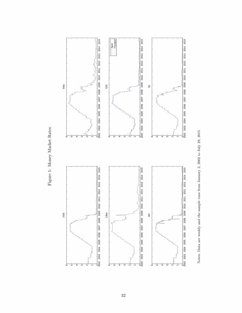
averages of daily series as of each Wednesday. The interest rates are plotted in figure 1 and

spreads are shown on figure 2. Table 1 reports descriptive statistics for the spreads. In what

follows, we discuss the properties and interpretation of each spread in more detail.2

The Libor-OIS spread likely has been one of the most closely watched indicators of funding

stress, especially since the onset of the financial crisis in the summer of 2007. Libor is the

average interest rate at which banks in London offer Eurodollars and it is a commonly referenced

benchmark of the short-term interest rate in the U.S. dollar market.3 The 3-month OIS rate is

1Although the Libor-OIS spread uses the spot OIS rate while 3x6 FRA-OIS relies on the forward OIS rate, weuse the same notation for the OIS leg in both cases for simplicity.

2See Stigum and Crescenzi (2007) for further information on money market rates and the underlying contracts.3Reports of possible misrepresentation of the Libor by certain banks emerged in 2008, see for example “Study

Casts Doubt on Key Rate”, Wall Street Journal, May 29, 2008. Such banks were later fined for attempting to

4

the average effective federal funds rate expected over the next 3 months, as reflected in overnight

index swaps. In an OIS, a fixed rate is swapped for the geometric average effective federal funds

rate over the contract period. The transaction involves only marginal counterparty risk since the

principal amount is not exchanged between the parties. Hence, the spread between Libor and the

OIS rate serves as a spot measure for both liquidity and credit risk premia. As illustrated in panel

A of figure 2, the Libor-OIS spread has generally been narrow and positive, reflecting the small

credit and liquidity risk premia inherent in the 3-month Libor. Before mid-2007, the spread had

been generally fluctuating around 10 basis points (table 1, first column). However, the average

increased to about 90 basis points from mid-2007 to mid-2009 and the spread reached as high

as 350 basis points in October 2008 following the Lehman Brothers bankruptcy. Since mid-2009,

the end of the Great Recession according to the NBER, the spread has been fluctuating around

19 basis points. Over the entire sample period, the spread averaged 26 basis points, and it has

generally been very persistent with a first order autocorrelation coefficient of 0.98.

The FRA-OIS spread can be thought of as the forward equivalent of the spot Libor-OIS

spread, as it reflects market expectations for funding conditions in the near future. A FRA is a

forward contract that determines the rate of interest between parties to be paid or received on

an obligation beginning at a future date. It is an interest rate swap with a single cash flow where

the underlying reference rate is the 3-month Libor, so it can also be thought of as the over-the-

counter equivalent of a Eurodollar futures contract. FRA transactions are mostly entered as a

hedge against future interest rate changes. For example, in a 3x6 FRA, the parties agree to trade

a specific amount of 3-month Eurodollars three months hence. At the settlement date, if the

market rate is higher than the contract rate, the seller pays the buyer the difference based on the

principal, or vice versa if the market rate is lower. Since the principal amount does not change

hands, there’s very little credit risk in FRA transactions. FRA-OIS is calculated as the spread

between the 3x6 FRA rate and the 3-month OIS rate 3-month forward. As expected, the averages

of the FRA-OIS spread over the full-sample period and the subsamples is fairly close to those

of the Libor-OIS spread (table 1, second column). Moreover, the persistence of the FRA-OIS

spread is also similar to the Libor-OIS although it is generally somewhat more volatile.

manipulate the Libor, see for example “EU Fines Financial Institutions Over Fixing Key Benchmarks”, WallStreet Journal, December 4, 2013. Nonetheless, Kuo et al. (2012) find that Libor survey responses broadly trackalternative measures between 2007-2009.

5

FFR-RP spread is the difference between the federal funds rate and the Treasury GC repo

rate. The federal funds market is an interbank, over-the-counter market for reserve balances,

with most transactions having an overnight term. The FFR is the average interest rate paid

on these unsecured loans of reserve balances held at the Federal Reserve Banks. Prior to the

global financial crisis, banks typically had relied on the federal funds market to satisfy reserve

requirements and other short-term liquidity needs. The Treasury GC repo rate is the rate on

secured overnight lending against collateral issued by the U.S. Treasury. Compared to the federal

funds market, the repo market has a wider array of participants since it brings together not only

banks, but also money market funds, securities broker-dealers, hedge funds, and other financial

institutions as well as nonfinancial corporations.

There exists a strong arbitrage connection between the federal funds market and the repo

market. When the RP is greater than FFR, lenders of funds can borrow collateral instead of

lending to other banks in the unsecured market. As a result, cash moves from the federal funds

market to the repo market, creating downward pressure on the RP rate and pushing the FFR up.

However, the arbitrage doesn’t work the other way, i.e. when RP is below FFR. Because, investors

demand for Treasury collateral cannot be substituted with an uncollateralized loan, keeping the

RP usually below the FFR. Therefore, the spread between the unsecured federal funds rate and

the overnight secured repo rate serves as a measure of counterparty or credit risk in overnight

funding markets. However, the spread between the two rates can be quite volatile over short

periods of time due to changes in the demand for and supply of Treasury collateral as well as

frictions related to financial reporting dates. Negative spread values have become considerably

more common since the FOMC reduced the FFR to its effective lower bound; the spread averaged

about 1 basis point since mid-2009 as opposed to about 5 basis points prior to the financial crisis

(table 1, third column). Persistence of the FFR-Repo spread is notably lower than that of the

other spreads, and it is relatively stable in the subsamples.

Several factors likely contributed to changing dynamics in the federal funds market during

the ZLB period. Afonso et al. (2013b) show that federal funds market trading volumes declined

significantly after the financial crisis against the backdrop of unprecedented levels of reserves

in the banking system and the introduction of interest payments on excess reserves (IOER) by

the Federal Reserve. The positive spread between the IOER and the effective FFR as well as

6

increased credit risk aversion by lenders also seem to have contributed to changes in the federal

funds market, see Afonso et al. (2013a), Afonso et al. (2011), and Bech and Klee (2011). The

changing regulatory environment seems to have played a role as well. For example, anecdotal

evidence suggests that leverage ratio constraints under Basel III are the primary reasons behind

banks’ reluctance to engage in arbitrage trades in the federal funds market.

The Libor-TB spread (also known as the TED spread) is calculated as the difference between

the 3-month Libor and the yield on the 3-month Treasury bill.4 It is a commonly used proxy for

risk appetite as it measures the perceived risk in lending to banks relative to investing in risk-free

Treasury bills. A rising TED spread may be indicative of a withdrawal of liquidity from funding

markets because of an increase in the perceived risk about the health of the banking system.

Even though this measure presumably captures risk dynamics similar to the Libor-OIS spread,

it also provides useful insights into flight-to-quality dynamics during times of stress since such

pressures may manifest themselves in decoupling of returns on Treasury securities from other

money market rates. The pre- and post-crisis averages of the TED spread are close at around 25

basis points (table 1, fourth column). Between mid-2007 and mid-2009, values above 150 basis

points were common and values as large as 300 basis points were observed in the aftermath of the

Lehman Brothers bankruptcy. Persistence characteristics of the TED spread are close to those

of the Libor-OIS and the FRA-OIS spreads.

3 Methodology

For a given spread, dynamics of the underlying pair of interest rates can be captured by a vector

error-correction (VEC) model where the spread serves as an error correction term. This is because

the two time series can both be approximated as I(1) processes, and they are not expected to

drift away from each other for a prolonged time due to arbitrage and policy intervention.5 Let yt

denote a 2× 1 vector of interest rates underlying a given spread. The linear VEC model with p

lags is given by,

∆yt = ΨXt + εt, (1)

4The TED spread used to be calculated as the difference between the 3-month Eurodollars contract and theyield on a 3-month Treasury bill until the Chicago Mercantile Exchange dropped Treasury bill futures followingthe 1987 crash.

5See 4.1 for unit root and cointegration tests.

7

where Ψ = (c, φ,A1, . . . , Ap), Xt = (1, st−1,∆y′t−1, . . . ,∆y

′t−p)

′, and st = y2,t − y1,t. The innova-

tion vector, εt, is assumed to be martingale difference with time-varying heteroskedasticity and

its elements are allowed to have non-zero contemporaneous correlation.

The linear VEC specification has important limitations. The model implicitly assumes that

deviations of the spread from its long-run equilibrium decrease at a pace that is independent of

the level of the spread. In practice, the speed of adjustment is more likely to be a function of

the magnitude of the spread. As the deviation from the long-run equilibrium becomes larger,

so does the profitability of arbitrage or the likelihood of policy intervention, which likely lead to

quicker adjustments back to equilibrium.6 Moreover, the tendency of the system to move toward

a long-run equilibrium may not even be present in every time period. Prolonged deviations from

long-run average values may hinder adjustment toward equilibrium and result in asymmetric

behavior over different time periods.7 Therefore, we allow for regime-switching in the parameters

of the VEC model to allow for discontinuous adjustment to equilibrium as well as other potential

asymmetries. We assume that the level of the lagged spread between the two rates, which serves

as the error correction term, also determines the regimes characterized by different dynamics.

The n-state threshold VEC (TVEC) model in this context can be written as follows:

∆yt =n∑j=1

ΨjXt1(γj−1 < st−1 ≤ γj) + εt, (2)

where Ψj =(cj , φj , A

j1, . . . , A

jp

). The parameters γjnj=0 are the threshold values such that

γ0 = −∞ and γs = ∞, and 1(·) is the standard indicator function. The model assumes that

there are n different regimes in which ∆yt follows a linear process, but the general dynamics of

∆yt over time are described by a nonlinear process. When n = 1, the threshold model boils down

to the linear model in equation 1.

We test for the threshold effects in the VEC model by considering the null hypothesis that

∆yt is linear (equation 1) against the alternative hypothesis that it follows a nonlinear process as

in equation 2. The presence of nuisance parameters that are undefined under the null hypothesis

6Several studies on the process of price discovery in financial markets, such as e.g. Dwyer et al. (1996), Martenset al. (1998), and Theissen (2012), find evidence of nonlinear adjustment dynamics between spot and futuresmarkets that can be modeled through nonlinear VEC models.

7See for example Balke and Fomby (1997) who argue that discrete adjustment processes describe the behaviorof many economic phenomena.

8

of linearity complicate the otherwise standard procedures of Wald or likelihood ratio testing. We

follow the recursive residual-based testing method of Tsay (1998) that produces easy to compute

test statistics with standard asymptotic distributions.

We estimate the threshold model using conditional least squares (CLS). Without loss of gen-

erality, let us illustrate the estimation procedure for the two-state case, i.e., n = 2, where the

model is given by,

∆yt = Ψ1Xt1(st−1 ≤ γ1) + Ψ2Xt1(st−1 > γ1) + εt.

Let Xt = (X ′t1(st−1 ≤ γ1) , X ′t1(st−1 > γ1))′ and Θ =

(Ψ1,Ψ2

), then the model can be compactly

written as ∆yt = ΘXt + εt. For a given value of the threshold, γ1, the CLS estimate of Θ is

defined as follows,

Θ′(γ1) =

[∑t

XtX′t

]−1 [∑t

Xty′t

].

Let εt = yt− Θ(γ1)Xt, then the total sum of squares (SSR) as a function of the threshold is given

by SSR(γ1) = tr (∑

t εtε′t) where tr(.) denotes the trace operator. Finally, the CLS estimate of

γ1 is obtained from

γ1 = argminγ1

SSR(γ1),

where γ1 ∈ R0, R0 ⊂ R, i.e. R0 is a bounded subset of the real line. In practice, we use a

symmetrically trimmed version of the set S = s1, . . . , sT−1. In particular, we consider trimming

percentages of 15, 10, and 5%. The resulting least squares estimate of Θ is Θ(γ1). In case of the

three-regime model, we estimate the first threshold with 15% trimming and then conduct another

grid search for the second threshold in a similar fashion with 5% trimming.

Inference on the parameters of the TVEC model is conducted via asymptotic methods and

subsampling. Because the threshold estimate converges at rate T , we treat the threshold as

known to conduct inference on Θ that converge at rate of√T . However, the distribution of

the threshold estimate is not asymptotically nuisance parameter free, so we use the subsampling

methods proposed by Politis et al. (1999) to construct asymptotically valid confidence intervals

for the threshold parameter(s), e.g. Gonzalo and Wolf (2005). Let b denote the block size such

that 1 < b < T ; we estimate the model on blocks yt, . . . , yt+b−1T−b+1t=1 . Assuming that b → ∞

9

and b/T → 0, the confidence interval based on estimates from the blocks has the desired coverage

probability. To satisfy this requirement we set b = d3T 1/2e where d.e is the ceiling function.

We estimate a multivariate GARCH model for the innovations from the TVEC model to

capture substantial volatility clustering in the data. We assume that volatility of the innovations

are fully time-varying, but their correlations are constant in each state after we account for het-

eroskedasticity. Therefore, our approach can be regarded as a hybrid of the constant conditional

correlation model of Bollerslev (1990) and the dynamic conditional correlation model of Engle

(2002).8 Specifically, let Ht = Cov(εt|Ωt−1), then we can write

Ht = DtRtDt,

where Dt = diag√

Var(εit|Ωt−1)

for i = 1, 2, Ωt denotes time t information, and Rt =

Corr(εt|Ωt−1). We consider the following threshold GARCH (1,1) specification for the elements

of Dt:

d2it = 1(γj−1 < st−1 ≤ γj)ωi,j + αiε2i,t−1 + βid

2i,t−1 (3)

where ωi,j = (1−αi−βi)σ2i,j and σ2i,j = E[ε2it | γj−1 < st−1 ≤ γj

]. Then the conditional correlation

at any point in time is simply the correlation coefficient of the resulting GARCH residuals in the

corresponding regime. Formally, let eit = εit/dit and ρj = E [e1,te2,t | γj−1 < st−1 ≤ γj ], then the

off-diagonal element of the conditional correlation matrix Rt, say ρt, is given by ρt = 1(γj−1 <

st−1 ≤ γj)ρj .

To cross-check the TVEC model estimates and further explore dynamics of the spreads, we

also estimate univariate threshold models for each of the four spreads. The first-order self-exciting

threshold autoregression (SETAR) model for the spreads is given by:

st =n∑j=1

δjzt1(γj−1 < st−1 ≤ γj) + ζt,

where zt = (1, st−1)′, δj = (µj , κj), and ζt is martingale difference with time-varying heteroskedas-

ticity, which is modeled via the threshold GARCH specification given in equation 3.

8Models that allow for time-varying correlations within each state are not supported by the data in any of thecases we analyze.

10

4 Empirical Results

4.1 Testing for Unit Root, Cointegration and Nonlinearity

As in Balke and Fomby (1997) we follow a two-step approach and first test for cointegration be-

tween money market rates and then explore potential nonlinearities in their long-run relationship.

Table 2 summarizes the results of the unit root tests for the six interest rate series and the four

spreads. Test statistics for the rates and spreads are reported in panels A and B, respectively, and

the critical values are given in panel C. We report the augmented version of the Dickey and Fuller

(1979) test (ADF), GLS-detrended Dickey-Fuller test (DF-GLS), the point optimal test of Elliott

et al. (1996) (ERS), the t-type test of Ng and Perron (2001) (NP), and the Phillips and Perron

(1988) test (PP). As can be seen from panel A, interest rates are well approximated by I(1) pro-

cesses over the full-sample since all test statistics agree at typical conventional significance levels

that the interest rate processes contain unit roots.9 The potential cointegrating relationship we

focus on crucially depends on the stationarity of the spread between the two interest rate series

in each case. Therefore, tests of cointegration boil down to tests of unit root for the spreads.

Tests statistics shown in panel B confirm our expectation that each pair is cointegrated over the

full-sample period where the corresponding spread serves as an error-correction term.

Table 3 summarizes the results of Tsay (1998)’s threshold nonlinearity test for the null of a

linear VEC against the TVEC where the stationary spreads serve as both the error correction

terms and the variables driving the regimes. The initial sample size used to start the recursion

is T0 =⌈cT 1/2

⌉where c = 2, but qualitatively similar results are obtained with c ∈ 3, 4, 5.

In case of a parsimonious first order model (p = 1), the null of linearity is strongly rejected for

all pairs with the exception of FRA-OIS. This result holds when the lag order is selected under

different information criteria (Akaike, Schwarz and Hannan-Quinn).10 However, we reject the

null at 10% significance level in case of the FRA-OIS pair when we choose the lag order with

respect to Akaike information criterion as in Tsay (1998).

9The KPSS test of Kwiatkowski et al. (1992) that assumes stationarity under the null leads to qualitativelysimilar results for both the interest rates and the spreads.

10We consider the maximum lag order of four because with p = 4 the linear VEC has a saturation ratio—thenumber of data points per parameter—of 71 which decreases to only 24 for the three regime TVEC.

11

Because the threshold nonlinearity test is not informative about the number of regimes, we

mainly rely on information criteria for this purpose, see Tsay (1998) for a similar approach for

threshold models and Guidolin and Timmermann (2006) for Markov-Switching models. As can

be seen from Table 4, for p = 1 all three information criteria favor threshold models over linear

models and the three-regime model over the two-regime model for all pairs of interest rates.

Additional findings that are not reported here to save space indicate that this result holds for

p > 1 as well. In addition, plots of SSR as a function of the threshold (not shown) also indicate

that the three-regime model is the preferred model. In what follows we focus on first-order TVEC

models with three regimes. 11

4.2 Threshold Estimates and Regimes

The threshold estimates and their subsampling-based confidence intervals at 90% level are shown

in panel A of table 5. Regime classifications from the TVEC models are plotted in Figures 3 to 6.

In these figures, panels A, B and C show the regime classification based on the lower bound of the

confidence interval for the threshold, its point estimate, and the upper bound of its confidence

interval, respectively. Unless otherwise noted, we will be referring to regime-classifications based

on the point estimates of the threshold parameters.

For the Libor-OIS spread, the low and high threshold estimates are 40 and 86 basis points,

respectively (table 5, panel A). The first regime can be regarded as a state of normal market

functioning in which the spread fluctuates at levels not far from the long-run mean. The second

regime is characterized by an increase in funding pressures, while in the third regime such pres-

sures reach high levels and market functioning may be substantially impaired. The width of the

symmetric confidence band for the low threshold is 20 basis points while that of the high thresh-

old is about 30 basis points. Relatively lower precision in the estimation of the high threshold is

likely due to extremely high volatility at the height of the crisis.

As for the dating of the regimes, the first regime had prevailed from the beginning of the

sample until August 2007, around the time BNP Paribas announced that it was ceasing activity

11Results under higher lag orders yield qualitatively similar results and are available upon request.

12

in three investment funds specialized in U.S. mortgage debt (figure 3, panel B).12 This announce-

ment seemed to be an important sign of the propagation of stress related to mortgage backed

securities in the broader financial system, and our analysis documents the regime-shift in the

money markets around that time. The second regime dominated the period that followed until

the widespread turmoil triggered by the Lehman Brothers bankruptcy in September 2008 took

place. The spread eventually declined and the system reverted back to the second regime in April

2009 as funding pressures subsided amid various unconventional policy measures undertaken by

the Federal Reserve. By mid-2009, the end of the recession according to the NBER, the Libor-

OIS spread reached levels consistent with the system being in the first regime. After this point,

there were two instances of relatively elevated spreads in the post-crisis period. The spread ap-

proached the lower bound of the confidence band for the first threshold in mid-2010, around the

time when the Greek government debt was downgraded to junk-bond status, and breached the

estimated threshold in late-2011 amid increased financial distress in Europe due to the sovereign

debt crisis. In both of these episodes the Federal Reserve expanded the swap facilities with other

major central banks to provide U.S. dollar liquidity to the offshore market, which seemed to help

bring the spread back to levels closer to its long-run average.

The FRA-OIS regimes can be interpreted in a similar fashion, i.e. normal, moderate-stress

and high-stress regimes. The point estimate for the first threshold is nearly identical to that of

Libor-OIS while the second threshold is estimated to be somewhat lower. In part because of this

difference, as can be seen from figure 4, the FRA-OIS pair entered the third regime earlier and

stayed in that regime longer compared with the Libor-OIS. Another notable difference is that the

FRA-OIS spread suggested a movement to the moderate-stress regime both in mid-2010 and late

2011 while the Libor-OIS estimates suggest a regime-shift only in 2011. Both in case of the high

stress regime that prevailed during the financial crisis and the moderate stress period associated

with the sovereign debt crisis in Europe, the FRA-OIS spread signaled a regime shift earlier than

the spot rate based Libor-OIS spread, emphasizing the forward looking nature of the former.

For the FFR-RP pair, the three regimes identified by two threshold estimates have different

interpretations than the above described cases. The first threshold estimate is practically zero, so

12Prior to this announcement, Standard and Poor’s and Moody’s had downgraded over 100 bonds backed bysubprime mortgages and hedge funds sponsored by Bear Sterns with investments in complex securities backed bysubprime mortgages had collapsed.

13

the first regime is associated with the relatively unusual case of the FFR printing below the RP

rate. Although this is typically observed only around financial reporting dates, consistent with the

changes in the federal funds market activity discussed above, it became much more common after

the reduction of the FFR to its effective lower bound in December 2008. The second threshold

estimate of 15 basis points distinguishes times of elevated funding pressures characterized by

the widening gap between unsecured and secured rates from times of usual market functioning

captured by the intermediate regime. Prior to the crisis, the spread has mostly fluctuated between

the two thresholds, with the exception of some short-lived jumps around quarter-end and year-

end dates where the FFR remained below the RP rate (figure 4). Most of the crisis period until

the beginning of the ZLB period in December 2008 is characterized by the third regime.

Finally, in case of the Libor-TB spread, plotted in figure 6, the threshold estimates, at 53 and

95 basis points respectively, are somewhat higher than the Libor-OIS spreads, likely reflecting

the effects of flight to quality flows on short-term Treasury yields. Nonetheless, the resulting

regime-classification is similar to the Libor-OIS case. A notable exception is the stress period in

late 2011 and early 2012: it is classified in the first regime with respect to the TED spread while

Libor-OIS indicates a shift to the intermediate stress regime.

As a robustness check, we also estimated SETAR models for each of the four spreads and

compared the threshold estimates with those coming from the TVEC models estimated for pairs

of rates. The threshold estimates and the corresponding confidence intervals from the first order

SETAR model are reported in panel B of Table 5. Comparison of these values with those reported

in panel A reveals that the two estimation methods generally produce very similar point and

interval estimates for the spread thresholds, resulting in similar regime classifications. The only

notable difference is observed in case of the FRA-OIS spread where the SETAR model produces

a somewhat lower point estimate for the first threshold, and as a result, a slightly different regime

classification.

4.3 Regime-dependent Equilibrium Dynamics

Tables 6 to 9 report parameter estimates of the T-VEC models for each pair of rates, respectively.

In each case, the subscripts 1 and 2 index the essentially risk-free base rate and the relatively

risky funding rate, respectively.

14

Table 6 shows parameter estimates for the Libor-OIS case. The speed of adjustment pa-

rameters are negative for both rates and statistically significant in the normal (first) and the

high-stress (third) regimes. In these two regimes, when the spread deviates from its long-run

average, both rates move in the same direction but the risky rate (the Libor) is more responsive.

In terms of economic significance, the magnitude of adjustment appears to be rather small in

the first regime. In particular, a 10 basis point deviation of the spread from its long-run mean

predicts only 0.2 basis point compression in the spread during the following week as a results

of the adjustment in the underlying rates. However, in the third regime, the same amount of

deviation from the long-run equilibrium implies an adjustment that is five-times bigger. Our

results also suggest presence of an economically meaningful adjustment mechanism in the second

regime as well, but the estimates are not significantly different from zero in the statistical sense.

Overall, the equilibrium adjustment is both economically and statistically significant only in case

of the third regime for the Libor-OIS case. The gradual adjustment in the high-stress state is

consistent with combined effects of unconventional policy tools that aimed to reduce risk spreads

and response of some market participants to the unusually high levels of compensation for taking

on additional risk. In addition, when we estimate a linear VEC model for the Libor-OIS pair, we

find that the implied equilibrium dynamics largely coincide with those of the first regime from

the nonlinear TVEC model.13 Hence, the linear model masks the statistically and economically

meaningful adjustment in the third-regime following large shocks to the system.

Parameter estimates for the FRA-OIS case are reported in Table 7. The adjustment param-

eters in the first regime are both statistically significant at 1% level but they have the same sign

and magnitude. Thus, an adjustment toward a long-run equilibrium is absent. In contrast, the

second regime is associated with an adjustment through changes in the FRA rate significant at

10% level. Specifically, a 10 basis points shock to the spread relative to its long-run average

predicts a decline of about 4 basis points in the FRA rate. In the high-stress regime, both rates

respond negatively to the error correction term and the implied responses are highly statistically

significant. In addition, the estimated adjustment is smaller in the third regime than that in the

moderate stress regime. Given a 10 basis points shock to the spread the OIS rate is projected to

13To save space we do not report the detailed estimates from the linear VEC model for Libor-OIS and the otherpairs. Those results are available upon request.

15

decline by 2 basis points while the FRA rate is expected to decline twice as much. Similar to the

case of Libor-OIS, the linear VEC model yields very different results. It is effectively an average

of the three regimes resulting in a statistically significant adjustment that is economically much

weaker.

For the FFR-Repo case shown in Table 8, the adjustment parameter in the repo equation

is always larger in magnitude, consistent with the monetary policy implementation mechanism.

Until late 2008, the effective FFR has been kept near the target rate through open market

operations, possibly limiting the adjustment of the federal funds rate in response to movements in

the repo market. Moreover, Bech et al. (2014) argue that the secured nature of repo transactions

makes participants more willing to exploit pricing anomalies, leading to adjustment to deviations

through the repo market, and not the federal funds market. Indeed, the one-way arbitrage

between the two markets discussed above (see section 2) is reflected in the coefficient estimates in

the first regime where the spreads is negative. Our point estimates suggest an approximately one-

to-one adjustment in terms of the total response of the two rates, with the sensitivity of the RP

rate being more than twice as large as that of the FFR. However, statistical significance is lacking

in the first regime. The second regime, which is characterized with a positive spread smaller than

15 basis points, also lacks in terms of statistical significance of the adjustment mechanism. The

adjustment is both economically and statistically significant only in the third regime where the

spread exceeds 15 basis points. Several episodes during the crisis period associated with elevated

levels of funding stress fall in this category. In this regime, a 10 basis point shock to the spread

predicts a 5 basis point rise in the RP rate and a 2 basis point decline in the FFR. In contrast,

the linear VEC implies adjustments of similar magnitudes in both rates and attributes a less

statistically significant role for the RP adjustments.

Finally, Table 9 reports results for the Libor-TB pair. In the first regime, an economically

small adjustment toward the long-run equilibrium takes place via an increase in the TB rate in

response to a positive deviation in the spread. Interestingly, once the system enters the second

regime, the TB rate is projected to decrease significantly further relative to the Libor suggesting

a further rise in the spread. Once the spread is sufficiently high and the system enters the third

regime, then a gradual adjustment back toward the long-run equilibrium is projected through

decreases in the Libor rate, as in the case of the Libor-OIS pair. The difference between the

16

Libor-OIS and Libor-TB cases in the moderate stress regime likely reflects the effects of flight-to-

quality flows during times of stress on Treasury yields, emphasizing the role of market liquidity

risk premium besides the traditional term premia and credit risk effects. As in the case of

the Libor-OIS pair, the linear VEC masks such complex dynamics and suggests a statistically

significant but economically small average adjustment in response to shocks to the spread.

4.4 Time-varying Volatility and Correlation

Table 10 reports the parameter estimates of the multivariate GARCH models. As before, the

subscripts 1 and 2 index the essentially risk-free base rate and the relatively risky funding rate,

respectively. In case of the Libor-OIS pair, the risky funding rate (Libor) has a larger reaction

parameter (α) in the individual GARCH equation and a slightly lower overall persistence in the

volatility process. The regime-dependent volatility drift parameters of the two rates are close

to each other in the first two-regimes, with both being larger in the second regime. However,

in the third regime, the OIS volatility drift slightly declines relative to the intermediate regime

while that for Libor moves up substantially. Indeed, the volatility drift for Libor monotonically

increases as a function of the spread. The estimates for regime-dependent volatility drifts for the

FRA-OIS case depict a similar picture: the risky rate is subject to a larger jump in volatility

when funding stress increases. However, the volatility drifts of the relatively safe rate tend to be

larger in case of both FFR-RP and Libor-TB pairs. This pattern is likely driven by the effects of

flight-to-quality flows and increased demand for Treasury collateral during times of stress.

Regarding conditional correlations, the underlying rates tend to exhibit moderate to large

positive correlation in the regime associated with normal market functioning. As funding stress

builds up, notable declines in the correlations are observed. In case of Libor-OIS, the regime-

dependent correlation coefficient declines substantially as the spread breaches the first threshold

and then turns negative in the third regime when funding stress reaches its maximum level. The

FRA-OIS and Libor-TB cases exhibit a similar pattern across the two regimes. For the FFR-RP

pair, the correlation during normal times of market functioning as represented by the second

regime is 0.66 and drops slightly when the spread between the two rates increases above 15 basis

points, i.e. in the third regime. However, in the first regime, which mostly represents FFR-RP

dynamics during part of the ZLB period, the correlation coefficient diminishes substantially to

17

0.2. This is mainly due to the federal funds rate being almost flat at the zero-lower bound.

Although the volatility of the federal funds rate was minimal during the entire ZLB period, the

RP rate continued to move with the factors that affect the demand for and supply of cash and

Treasury collateral.

All rates exhibit increases in volatilities to unprecedented levels during the financial crisis

(figure 7). Volatilities also increased notably in the aftermath of the crisis during times of elevated

uncertainty in the offshore U.S. dollar funding markets in 2010 and 2011, but such increases were

considerably smaller than the movements observed at the height of the crisis. The volatility of

the RP and FFR reverted back to pre-crisis levels at the beginning of 2009 and declined further

in mid-2010 amid substantially reduced volume in the federal funds market. Overall, the RP rate

has been more volatile than the FFR during the ZLB period as it responds to factors such as

the demand for and supply of Treasury securities. Meanwhile, the TB rate volatility reached its

highest level during the ZLB period amid the government shutdown in October 2013.

The estimated volatilities of the spreads are plotted in figure 8. Consistent with the volatilities

of the rates, level shifts seem to drive most of the crisis period movements and the aforementioned

moderate stress episodes during the ZLB period. Since early 2009, spread volatilities generally

has been at levels close to or somewhat below their pre-crisis levels. In case of the FRA-OIS

spread, the stress in the offshore U.S. dollar funding markets in 2010 and 2011 produced larger

and more persistent movements in the estimated volatility series, perhaps reflecting lingering

uncertainty about funding conditions in the near-future.

5 Conclusion

We model dynamics of money market rates underlying the commonly-monitored spreads in a

threshold-error-correction framework where the spreads serve as both equilibrium correction terms

and the threshold variables identifying regimes with different dynamics. We provide estimates

and subsampling-based confidence intervals for spread thresholds to quantify funding pressure

points from a long-run perspective and identify regimes associated with different levels of fund-

ing stress. Our results indicate strong asymmetry in the equilibrium adjustment mechanism in

all considered segments of the money market, with cointegrating relationships breaking down in

18

certain regimes. The most economically significant adjustments take place in regimes associated

with high risk spreads, likely reflecting a combination of market response to high levels of com-

pensation for additional risk and policy intervention. In addition, allowing for regime-dependent

behavior in multivariate GARCH models fitted to the TVEC residuals, we quantify abrupt shifts

in interest rate volatilities as well as significant declines in their correlations in high spread regimes

characterized by elevated funding stress in money markets.

19

References

Afonso, G., A. Entz, and E. LeSueur (2013a): “Who’s Borrowing in the

Fed Funds Market,” http://libertystreeteconomics.newyorkfed.org/2013/12/

whos-borrowing-in-the-fed-funds-market.html, Liberty Street Economics Blog.

——— (2013b): “Who’s Lending in the Fed Funds Market,” http://libertystreeteconomics.

newyorkfed.org/2013/12/whos-lending-in-the-fed-funds-market.html, Liberty Street

Economics Blog.

Afonso, G., A. Kovner, and A. Schoar (2011): “Stressed, Not Frozen: The Federal Funds

Market in the Financial Crisis,” Journal of Finance, 66, 1109–1139.

Balke, N. S. and T. B. Fomby (1997): “Threshold Cointegration,” International Economic

Review, 38, 627–645.

Bech, M. and E. Klee (2011): “The Mechanics of a Graceful Exit: Interest on Reserves and

Segmentation in the Federal Funds Market,” Journal of Monetary Economics, 58, 415–431.

Bech, M., E. Klee, and V. Stebunovs (2014): “Arbitrage, Liquidity and Exit: The Repo

and Federal Funds Markets before, during, and Emerging from the Financial Crisis,” in De-

velopments in Macro-Finance Yield Curve Modelling, ed. by J. S. Chadha, A. C. J. Durre,

M. A. S. Joyce, and L. Sarno, Cambridge: Cambridge University Press, 293–325.

Bollerslev, T. (1990): “Modelling the Coherence in Short-run Nominal Exchange Rates: A

Multivariate Generalized ARCH Model,” The Review of Economics and Statistics, 498–505.

Bollerslev, T. and J. M. Wooldridge (1992): “Quasi-maximum Likelihood Estimation

and Inference in Dynamic Models with Time-varying Covariances,” Econometric Reviews, 11,

143–172.

Brunnermeier, M. K. and Y. Sannikov (2014): “A Macroeconomic Model with a Financial

Sector,” American Economic Review, 104, 379–421.

Carlson, M., T. King, and K. Lewis (2011): “Distress in the Financial Sector and Economic

Activity,” The B.E. Journal of Economic Analysis & Policy, 11, 1–31.

20

http://libertystreeteconomics.newyorkfed.org/2013/12/whos-borrowing-in-the-fed-funds-market.html

http://libertystreeteconomics.newyorkfed.org/2013/12/whos-borrowing-in-the-fed-funds-market.html

http://libertystreeteconomics.newyorkfed.org/2013/12/whos-lending-in-the-fed-funds-market.html

http://libertystreeteconomics.newyorkfed.org/2013/12/whos-lending-in-the-fed-funds-market.html

Carpenter, S., S. Demiralp, B. Schlusche, and Z. Senyuz (2014): “Measuring Stress in

Money Markets: A Dynamic Factor Approach,” Economics Letters, 125, 101–106.

Dickey, D. A. and W. A. Fuller (1979): “Distribution of the Estimators for Autoregressive

Time Series with A Unit Root,” Journal of the American statistical association, 74, 427–431.

Dwyer, G., P. Locke, and W. Yu (1996): “Index Arbitrage and Nonlinear Dynamics between

the S&P 500 Futures and Cash,” Review of Financial Studies, 9, 301–332.

Elliott, G., T. J. Rothenberg, and J. H. Stock (1996): “Efficient Tests for an Autore-

gressive Unit Root,” Econometrica, 64, 813–836.

Engle, R. (2002): “Dynamic Conditional Correlation: A Simple Class of Multivariate General-

ized Autoregressive Conditional Heteroskedasticity Models,” Journal of Business & Economic

Statistics, 20, 339–350.

Gonzalo, J. and M. Wolf (2005): “Subsampling Inference in Threshold Autoregressive Mod-

els,” Journal of Econometrics, 127, 201–224.

Guidolin, M. and A. Timmermann (2006): “An Econometric Model of Nonlinear Dynamics

in the Joint Distribution of Stock and Bond Returns,” Journal of Applied Econometrics, 21,

1–22.

Hakkio, C. S. and W. R. Keeton (2009): “Financial stress: What is it, How can it be

Measured, and Why does it Matter?” Federal Reserve Bank of Kansas City Economic Review,

Second Quarter, 5–50.

He, Z. and A. Krishnamurthy (2012): “A Model of Capital and Crises,” Review of Economic

Studies, 79, 735–777.

Ivashina, V., D. S. Scharfstein, and J. C. Stein (2015): “Dollar Funding and the Lending

Behavior of Global Banks,” The Quarterly Journal of Economics, 130, 1241–1281.

Kuo, D., D. Skeie, and J. Vickery (2012): “A Comparison of Libor to Other Measures of

Bank Borrowing Costs,” Mimeo.

21

Kwiatkowski, D., P. C. Phillips, P. Schmidt, and Y. Shin (1992): “Testing the Null

Hypothesis of Stationarity against the Aalternative of a Unit Root: How Sure are We that

Economic Time Series have a Unit Root?” Journal of econometrics, 54, 159–178.

Martens, M., P. Kofman, and T. C. F. Vorst (1998): “A Threshold Error-correction Model

for Intraday Futures and Index Returns,” Journal of Applied Econometrics, 13, 245–263.

Newey, W. K. and K. D. West (1987): “A Simple, Positive Semi-Definite, Heteroskedasticity

and Autocorrelation Consistent Covariance Matrix,” Econometrica, 703–08.

Ng, S. and P. Perron (2001): “Lag Length Selection and the Construction of Unit Root Tests

with Good Size and Power,” Econometrica, 69, 1519–1554.

Oet, M., R. Eiben, T. Bianco, D. Gramlich, and S. Ong (2011): “The Financial Stress In-

dex: Identification of Systemic Risk Conditions,” Federal Reserve Bank of Cleveland, Working

Paper no. 1130.

Phillips, P. C. and P. Perron (1988): “Testing for a Unit Root in Time Series Regression,”

Biometrika, 75, 335–346.

Politis, D., J. Romano, and M. Wolf (1999): Subsampling, Springer.

Stigum, M. and A. Crescenzi (2007): Stigum’s Money Market, New York: McGraw-Hill, 4

ed.

Theissen, E. (2012): “Price Discovery in Spot and Futures Markets: A reconsideration,” Euro-

pean Journal of Finance, 18, 969–987.

Tsay, R. S. (1998): “Testing and Modeling Multivariate Threshold Models,” Journal of the

American Statistical Association, 93, 1188–1202.

Vayanos, D. (2004): “Flight to Quality, Flight to Liquidity, and the Pricing of Risk,” NBER

Working Paper Series, No. 10327.

22

Tables and Figures

Table 1: Descriptive Statistics for Money Market Spreads

Libor-OIS FRA-OIS FFR-RP Libor-TB

Panel A: January 2, 2002-June 27, 2007

Mean 11.0 11.2 5.1 26.3IQR 4.7 6.0 5.6 14.4AC(1) 0.93 0.94 0.62 0.95

Panel B: July 3, 2007-June 24, 2009

Mean 89.9 69.2 19.8 130.6IQR 36.0 41.4 25.7 58.5AC(1) 0.95 0.96 0.58 0.92

Panel C: July 1, 2009-July 29, 2015

Mean 18.6 22.4 1.3 24.7IQR 8.1 11.2 4.4 7.7AC(1) 0.99 0.97 0.73 0.98

Panel D: January 2, 2002-July 29, 2015

Mean 25.9 24.7 5.6 40.8IQR 12.2 14.7 5.4 18.8AC(1) 0.98 0.98 0.65 0.97

Notes: Data are weekly. Mean and interquartile range (IQR) are re-

ported in basis points. AC(1) denotes first order autocorrelation. FFR

is the overnight federal funds rate, FRA is the rate on 3-month/6-month

forward rate agreements, Libor is the 3-month London interbank offered

rate, OIS is the 3-month overnight index swap rate, RP is is the rate on

overnight Treasury general collateral repurchase agreements, and TB is

the rate on 3-month Treasury bill the in secondary market.

23

Table 2: Unit Root Tests

ADF DFGLS NP PP ERS

Panel A: Interest Rates

OIS -0.97 -0.93 -0.93 -0.81 11.37Libor -0.68 -0.65 -0.66 -0.71 17.66OIS (forward) -0.86 -0.78 -0.78 -0.83 14.73FRA -0.60 -0.53 -0.53 -0.76 22.13RP -1.01 -0.92 -0.95 -0.75 10.67FFR -1.31 -1.26 -1.31 -0.80 6.59TB -0.60 -0.47 -0.47 -0.75 23.28

Panel B: Spreads

Libor-OIS -3.68 -3.17 -3.21 -2.92 0.96FRA-OIS -2.69 -2.65 -2.64 -2.52 1.76FFR-RP -5.70 -4.02 -3.98 -12.46 0.46Libor-TB -3.14 -2.71 -2.74 -3.12 1.60

Panel C: Critical Values

1% c.v. -3.44 -2.57 -2.58 -3.44 1.995% c.v. -2.87 -1.94 -1.98 -2.87 3.2610% c.v. -2.57 -1.62 -1.62 -2.57 4.48

Notes: ADF is the augmented Dickey and Fuller (1979) test statistic,

DFGLS is the GLS-detrended Dickey-Fuller test statistic, ERS is the

point optimal test statistic of Elliott et al. (1996), NP is the t-type test

of Ng and Perron (2001), and PP is the Phillips and Perron (1988) test.

24

Table 3: Threshold Nonlinearity Tests


p = 1 0.008 0.306 0.000 0.000p = pAIC 0.047 0.097 0.000 0.023p = pSIC 0.047 0.306 0.000 0.001p = pHQIC 0.047 0.306 0.000 0.023

Notes: p-values associated with the threshold nonlinearity test statis-

tics of Tsay (1998) are reported. p denotes the lag order in the linear

VEC model assumed under the null. AIC stands for Akaike informa-

tion criterion, SIC stands for Schwarz information criterion, and HQIC

stands for Hannan-Quinn information criterion. Data are weekly and

the sample runs from January 2, 2002 to July 29, 2015.

Table 4: Model Selection


Akaike

Linear VEC -7.1194 -7.1194 -3.7676 -5.12242-regime TVEC -8.2699 -8.2699 -5.0189 -7.58373-regime TVEC -9.5006 -9.5006 -5.8525 -8.2323

Schwarz


Hannan-Quinn


Notes: Model selection criteria for linear and threshold VEC models with

p = 1 are reported. Data are weekly and the sample runs from January 2,

2002 to July 29, 2015.

25

Table 5: Threshold Estimates and Subsampling Confidence Intervals

CIL(γ1) γ1 CIU (γ1) CIL(γ2) γ2 CIU (γ2)

Panel A: TVEC Model

Libor-OIS 30.4 40.0 49.5 70.7 86.3 101.9FRA-OIS 34.1 41.2 48.4 54.6 63.0 71.3FFR-RP -5.1 -0.6 3.9 8.8 15.2 21.6Libor-TB 43.3 52.6 61.9 75.8 95.2 114.6

Panel B: SETAR Model

Libor-OIS 30.1 40.0 49.9 76.5 87.9 99.3FRA-OIS 18.3 27.0 35.7 54.7 63.0 71.3FFR-RP -3.16 -1.6 0.0 7.7 14.2 20.7Libor-TB 42.8 52.6 62.5 84.1 100.0 115.9

Notes: Threshold estimates and 90% subsampling confidence intervals (in basis

points) are reported for TVEC and SETAR models with p = 1. Data are weekly

and the sample runs from January 2, 2002 to July 29, 2015.

26

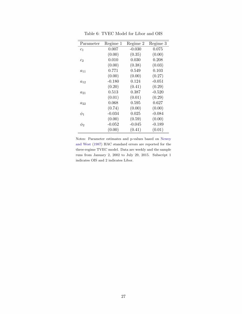
Table 6: TVEC Model for Libor and OIS

Parameter Regime 1 Regime 2 Regime 3

c1 0.007 -0.030 0.075(0.00) (0.35) (0.00)

c2 0.010 0.030 0.208(0.00) (0.38) (0.03)

a11 0.771 0.549 0.103(0.00) (0.00) (0.27)

a12 -0.180 0.124 -0.051(0.20) (0.41) (0.29)

a21 0.513 0.387 -0.520(0.01) (0.01) (0.29)

a22 0.068 0.595 0.627(0.74) (0.00) (0.00)

φ1 -0.034 0.025 -0.084(0.00) (0.59) (0.00)

φ2 -0.052 -0.045 -0.189(0.00) (0.41) (0.01)

Notes: Parameter estimates and p-values based on Newey

and West (1987) HAC standard errors are reported for the

three-regime TVEC model. Data are weekly and the sample

runs from January 2, 2002 to July 29, 2015. Subscript 1

indicates OIS and 2 indicates Libor.

27

Table 7: TVEC Model for FRA and OIS


c1 0.019 -0.016 0.164(0.00) (0.75) (0.00)

c2 0.021 0.179 0.338(0.00) (0.08) (0.00)

a11 0.231 0.124 -0.012(0.21) (0.29) (0.94)

a12 0.216 -0.038 0.128(0.18) (0.69) (0.07)

a21 0.152 -0.079 -0.786(0.33) (0.64) (0.14)

a22 0.279 0.248 0.438(0.07) (0.06) (0.04)

φ1 -0.121 0.018 -0.202(0.00) (0.87) (0.00)

φ2 -0.122 -0.392 -0.407(0.00) (0.07) (0.00)





indicates OIS and 2 indicates FRA.

28

Table 8: TVEC Model for FFR and RP


c1 0.011 -0.001 -0.185(0.58) (0.84) (0.04)

c2 -0.006 0.004 -0.009(0.59) (0.24) (0.84)

a11 -0.434 -0.266 0.302(0.16) (0.11) (0.01)

a12 1.367 0.166 0.055(0.02) (0.33) (0.81)

a21 -0.213 -0.024 -0.029(0.25) (0.81) (0.69)

a22 -0.010 0.003 -0.048(0.96) (0.98) (0.72)

φ1 0.777 0.187 0.487(0.29) (0.12) (0.02)

φ2 -0.310 0.045 -0.206(0.38) (0.67) (0.07)





indicates RP and 2 indicates FFR.

29

Table 9: TVEC Model for Libor and TB


c1 -0.009 0.246 -0.063(0.06) (0.01) (0.19)

c2 -0.002 0.024 0.108(0.54) (0.07) (0.03)

a11 0.376 1.058 -0.038(0.00) (0.00) (0.83)

a12 0.170 -1.326 0.199(0.04) (0.04) (0.11)

a21 0.093 0.212 -0.143(0.03) (0.00) (0.08)

a22 0.598 0.599 0.716(0.00) (0.00) (0.00)

φ1 0.040 -0.393 0.023(0.05) (0.00) (0.36)

φ2 0.014 -0.044 -0.088(0.19) (0.02) (0.01)





indicates TB and 2 indicates Libor.

30

Table 10: Multivariate GARCH Model


α1 0.297 0.182 0.159 0.201(0.00) (0.00) (0.00) (0.00)

α2 0.455 0.139 0.197 0.225(0.00) (0.00) (0.00) (0.00)

β1 0.668 0.809 0.830 0.789(0.00) (0.00) (0.00) (0.00)

β2 0.498 0.851 0.793 0.765(0.00) (0.00) (0.00) (0.00)

σ1,1 0.020 0.048 0.120 0.032σ2,1 0.019 0.050 0.067 0.019σ1,2 0.070 0.060 0.055 0.125σ2,2 0.082 0.081 0.049 0.030σ1,3 0.050 0.073 0.400 0.194σ2,3 0.171 0.128 0.216 0.151ρ1 0.495 0.863 0.219 0.228ρ2 0.177 0.627 0.656 0.498ρ3 -0.177 0.392 0.588 -0.022

Notes: p-values for GARCH parameters are based on Bollerslev

and Wooldridge (1992) robust standard errors. In case of Libor-

OIS, subscript 1 indicates OIS and 2 indicates Libor; in case of

FRA-OIS, subscript 1 indicates OIS and 2 indicates FRA; in case

of FFR-RP, subscript 1 indicates RP and 2 indicates FFR; in

case of Libor-TB, subscript 1 indicates TB and 2 indicates Libor.

For the regime-switching parameters (σi,j and ρj), i indexes rates

j indexes regimes. Data are weekly and the sample runs from

January 2, 2002 to July 29, 2015.

31

Fig

ure

1:M

oney

Mar

ket

Rat

es

2002

2003

2004

2005

2006

2007

2008

2009

2010

2011

2012

2013

2014

2015

0123456F

FR

2002

2003

2004

2005

2006

2007

2008

2009

2010

2011

2012

2013

2014

2015

0123456F

RA

2002

2003

2004

2005

2006

2007

2008

2009

2010

2011

2012

2013

2014

2015

0123456Li

bor

2002

2003

2004

2005

2006

2007

2008

2009

2010

2011

2012

2013

2014

2015

0123456O

IS

Spo

tF

orw

ard

2002

2003

2004

2005

2006

2007

2008

2009

2010

2011

2012

2013

2014

2015

0123456R

P

2002

2003

2004

2005

2006

2007

2008

2009

2010

2011

2012

2013

2014

2015

0123456T

B

Note

s:D

ata

are

wee

kly

and

the

sam

ple

runs

from

January

2,

2002

toJuly

29,

2015.

32

Fig

ure

2:M

oney

Mar

ket

Sp

read

s

2002

2003

2004

2005

2006

2007

2008

2009

2010

2011

2012

2013

2014

2015

0

0.51

1.52

2.53

3.5

Libo

r−O

IS

2002

2003

2004

2005

2006

2007

2008

2009

2010

2011

2012

2013

2014

2015

0

0.2

0.4

0.6

0.81

1.2

1.4

1.6

FR

A−

OIS

f

2002

2003

2004

2005

2006

2007

2008

2009

2010

2011

2012

2013

2014

2015

−0.

50

0.51

1.52

FF

R−

RP

2002

2003

2004

2005

2006

2007

2008

2009

2010

2011

2012

2013

2014

2015

0

0.51

1.52

2.53

3.54

4.5

Libo

r−T

B

Note

s:D

ata

are

wee

kly

and

the

sam

ple

runs

from

January

2,

2002

toJuly

29,

2015.

33

Figure 3: Regime Classification from the TVEC Model for Libor-OIS

2002 2003 2004 2005 2006 2007 2008 2009 2010 2011 2012 2013 2014 20150

0.5

1

1.5

2

2.5

3

3.5

4Panel A: Lower Bound of the Confidence Interval

Regime 1Regime 2Regime 3

2002 2003 2004 2005 2006 2007 2008 2009 2010 2011 2012 2013 2014 20150

0.5

1

1.5

2

2.5

3

3.5

4Panel B: Point Estimate


2002 2003 2004 2005 2006 2007 2008 2009 2010 2011 2012 2013 2014 20150

0.5

1

1.5

2

2.5

3

3.5

4Panel C: Upper Bound of the Confidence Interval


Notes: Data are weekly and the sample runs from January 2, 2002 to July 29, 2015.

34

Figure 4: Regime Classification from the TVEC Model for FRA-OIS

2002 2003 2004 2005 2006 2007 2008 2009 2010 2011 2012 2013 2014 20150

0.2

0.4

0.6

0.8

1

1.2

1.4

1.6

1.8



2002 2003 2004 2005 2006 2007 2008 2009 2010 2011 2012 2013 2014 20150

0.2

0.4

0.6

0.8

1

1.2

1.4

1.6

1.8



2002 2003 2004 2005 2006 2007 2008 2009 2010 2011 2012 2013 2014 20150

0.2

0.4

0.6

0.8

1

1.2

1.4

1.6

1.8




35

Figure 5: Regime Classification from the TVEC Model for FFR-RP

2002 2003 2004 2005 2006 2007 2008 2009 2010 2011 2012 2013 2014 2015−0.5

0

0.5

1

1.5



2002 2003 2004 2005 2006 2007 2008 2009 2010 2011 2012 2013 2014 2015−0.5

0

0.5

1

1.5



2002 2003 2004 2005 2006 2007 2008 2009 2010 2011 2012 2013 2014 2015−0.5

0

0.5

1

1.5




36

Figure 6: Regime Classification from the TVEC Model for Libor-TB

2002 2003 2004 2005 2006 2007 2008 2009 2010 2011 2012 2013 2014 20150

0.5

1

1.5

2

2.5

3

3.5

4

4.5



2002 2003 2004 2005 2006 2007 2008 2009 2010 2011 2012 2013 2014 20150

0.5

1

1.5

2

2.5

3

3.5

4

4.5



2002 2003 2004 2005 2006 2007 2008 2009 2010 2011 2012 2013 2014 20150

0.5

1

1.5

2

2.5

3

3.5

4

4.5




37

Fig

ure

7:E

stim

ated

Vol

atil

ity

Ser

ies

for

Inte

rest

Rat

es

2003

2004

2005

2006

2007

2008

2009

2010

2011

2012

2013

2014

2015

10−

3

10−

2

10−

1

100

Pan

el A

: Lib

or−

OIS

OIS

Libo

r

2003

2004

2005

2006

2007

2008

2009

2010

2011

2012

2013

2014

2015

10−

2

10−

1

100

Pan

el B

: FR

A−

OIS

OIS

FR

A

2003

2004

2005

2006

2007

2008

2009

2010

2011

2012

2013

2014

2015

10−

2

10−

1

100

Pan

el C

: FF

R−

RP

RP

FF

R

2003

2004

2005

2006

2007

2008

2009

2010

2011

2012

2013

2014

2015

10−

3

10−

2

10−

1

100

Pan

el D

: Lib

or−

TB

TB

Libo

r

Note

s:W

eekly

vola

tility

seri

esare

show

nfr

om

January

15,

2003

toJuly

29,

2015

on

alo

g-s

cale

.V

ola

tility

seri

esare

obta

ined

from

the

mult

ivari

ate

thre

shold

-GA

RC

Hm

odel

des

crib

edin

the

text.

38

Fig

ure

8:E

stim

ated

Vol

atil

ity

Ser

ies

for

Sp

read

s

2003

2004

2005

2006

2007

2008

2009

2010

2011

2012

2013

2014

2015

10−

3

10−

2

10−

1

100

Pan

el A

: Lib

or−

OIS

2003

2004

2005

2006

2007

2008

2009

2010

2011

2012

2013

2014

2015

10−

3

10−

2

10−

1

100

Pan

el B

: FR

A−

OIS

2003

2004

2005

2006

2007

2008

2009

2010

2011

2012

2013

2014

2015

10−

2

10−

1

100

Pan

el C

: FF

R−

RP

2003

2004

2005

2006

2007

2008

2009

2010

2011

2012

2013

2014

2015

10−

3

10−

2

10−

1

100

Pan

el D

: Lib

or−

TB

Note

s:W

eekly

vola

tility

seri

esare

show

nfr

om

January

15,

2003

toJuly

29,

2015

on

alo

g-s

cale

.V

ola

tility

seri

esare

obta

ined

from

the

thre

shold

-GA

RC

Hm

odel

des

crib

edin

the

text.

39

Financial Stress and Equilibrium Dynamics in Money Markets · · 2015-10-15Financial Stress and...

Documents

Transcript of Financial Stress and Equilibrium Dynamics in Money Markets · · 2015-10-15Financial Stress and...