To Appear in the in 2002 in the volume

‘‘Heavy-tailed distributions in Finance’’, Svetlozar T. Rachev, editor, North Holland

Copyright Brendan O. Bradley and Murad S. Taqqu

Financial Risk and Heavy Tails

Brendan O. Bradley and Murad S. TaqquBoston University

August 28, 2001

Abstract

It is of great importance for those in charge of managing risk to understand how financial assetreturns are distributed. Practitioners often assume for convenience that the distribution is normal.Since the 1960s, however, empirical evidence has led many to reject this assumption in favor ofvarious heavy-tailed alternatives. In a heavy-tailed distribution the likelihood that one encounterssignificant deviations from the mean is much greater than in the case of the normal distribution.It is now commonly accepted that financial asset returns are, in fact, heavy-tailed. The goal of thissurvey is to examine how these heavy tails affect several aspects of financial portfolio theory andrisk management. We describe some of the methods that one can use to deal with heavy tails andwe illustrate them using the NASDAQ composite index.

1

Contents

1 Introduction 4

2 Historical Perspective 52.1 Risk and Utility . . . . . . . . . . . . . . . . . . . . . . . . . . . . . . . . . . . . . . . . 52.2 Markowitz Mean-Variance Portfolio Theory . . . . . . . . . . . . . . . . . . . . . . . . 52.3 CAPM and APT . . . . . . . . . . . . . . . . . . . . . . . . . . . . . . . . . . . . . . . 62.4 Empirical Evidence . . . . . . . . . . . . . . . . . . . . . . . . . . . . . . . . . . . . . . 9

3 Value at Risk 103.1 Computation of VaR . . . . . . . . . . . . . . . . . . . . . . . . . . . . . . . . . . . . . 13

3.1.1 Historical Simulation VaR . . . . . . . . . . . . . . . . . . . . . . . . . . . . . . 133.1.2 Parametric VaR . . . . . . . . . . . . . . . . . . . . . . . . . . . . . . . . . . . 143.1.3 Monte Carlo VaR . . . . . . . . . . . . . . . . . . . . . . . . . . . . . . . . . . 16

3.2 Parameter Estimation . . . . . . . . . . . . . . . . . . . . . . . . . . . . . . . . . . . . 173.2.1 Historical Volatility . . . . . . . . . . . . . . . . . . . . . . . . . . . . . . . . . 173.2.2 ARCH/GARCH Volatilities . . . . . . . . . . . . . . . . . . . . . . . . . . . . . 193.2.3 Implied Volatilities . . . . . . . . . . . . . . . . . . . . . . . . . . . . . . . . . . 223.2.4 Extreme Value Theory . . . . . . . . . . . . . . . . . . . . . . . . . . . . . . . . 22

4 Risk Measures 234.1 Coherent Risk Measures . . . . . . . . . . . . . . . . . . . . . . . . . . . . . . . . . . . 234.2 Expected Shortfall . . . . . . . . . . . . . . . . . . . . . . . . . . . . . . . . . . . . . . 24

5 Portfolios and Dependence 255.1 Copulas . . . . . . . . . . . . . . . . . . . . . . . . . . . . . . . . . . . . . . . . . . . . 265.2 Measures of Dependence . . . . . . . . . . . . . . . . . . . . . . . . . . . . . . . . . . . 30

5.2.1 Linear Correlation . . . . . . . . . . . . . . . . . . . . . . . . . . . . . . . . . . 315.2.2 Rank Correlation . . . . . . . . . . . . . . . . . . . . . . . . . . . . . . . . . . . 315.2.3 Comonotonicity . . . . . . . . . . . . . . . . . . . . . . . . . . . . . . . . . . . . 325.2.4 Tail Dependence . . . . . . . . . . . . . . . . . . . . . . . . . . . . . . . . . . . 33

5.3 Elliptical Distributions . . . . . . . . . . . . . . . . . . . . . . . . . . . . . . . . . . . . 35

6 Univariate Extreme Value Theory 396.1 Limit Law for Maxima . . . . . . . . . . . . . . . . . . . . . . . . . . . . . . . . . . . . 406.2 Block Maxima Method . . . . . . . . . . . . . . . . . . . . . . . . . . . . . . . . . . . . 416.3 Using the Block Maxima Method for Stress Testing . . . . . . . . . . . . . . . . . . . . 436.4 Peaks Over Threshold Method . . . . . . . . . . . . . . . . . . . . . . . . . . . . . . . 44

6.4.1 Semiparametric Approach . . . . . . . . . . . . . . . . . . . . . . . . . . . . . . 446.4.2 Fully Parametric Approach . . . . . . . . . . . . . . . . . . . . . . . . . . . . . 466.4.3 Numerical Illustration . . . . . . . . . . . . . . . . . . . . . . . . . . . . . . . . 506.4.4 A GARCH-EVT model for Risk . . . . . . . . . . . . . . . . . . . . . . . . . . 51

2

7 Stable Paretian Models 547.1 Stable Portfolio Theory . . . . . . . . . . . . . . . . . . . . . . . . . . . . . . . . . . . 557.2 Stable Asset Pricing . . . . . . . . . . . . . . . . . . . . . . . . . . . . . . . . . . . . . 57

3

1 Introduction

Financial theory has long recognized the interaction of risk and reward. The seminal work of Markowitz[Mar52] made explicit the trade-off of risk and reward in the context of a portfolio of financial assets.Others such as Sharpe [Sha64], Lintner [Lin65], and Ross [Ros76], have used equilibrium arguments todevelop asset pricing models such as the capital asset pricing model (CAPM) and the arbitrage pricingtheory (APT), relating the expected return of an asset to other risk factors. A common theme of thesemodels is the assumption of normally distributed returns. Even the classic Black and Scholes optionpricing theory [BS73] assumes that the return distribution of the underlying asset is normal. Theproblem with these models is that they do not always comport with the empirical evidence. Financialasset returns often possess distributions with tails heavier than those of the normal distribution.As early as 1963, Mandelbrot [Man63] recognized the heavy-tailed, highly peaked nature of certainfinancial time series. Since that time many models have been proposed to model heavy-tailed returnsof financial assets.

The implication that returns of financial assets have a heavy-tailed distribution may be profoundto a risk manager in a financial institution. For example, 3σ events may occur with a much largerprobability when the return distribution is heavy-tailed than when it is normal. Quantile basedmeasures of risk, such as value at risk, may also be drastically different if calculated for a heavy-taileddistribution. This is especially true for the highest quantiles of the distribution associated with veryrare but very damaging adverse market movements.

This paper serves as a review of the literature. In Section 2, we examine financial risk from anhistorical perspective. We review risk in the context of the mean-variance portfolio theory, CAPM andthe APT, and briefly discuss the validity of their assumption of normality. Section 3 introduces thepopular risk measure called value at risk (VaR). The computation of VaR often involves estimating ascale parameter of a distribution. This scale parameter is usually the volatility of the underlying asset.It is sometimes regarded as constant, but it can also be made to depend on the previous observationsas in the popular class of ARCH/GARCH models.

In Section 4, we discuss the validity of several risk measures by reviewing a proposed set ofproperties suggested by Artzner, Delbean, Eber and Heath [ADEH99] that any sensible risk measureshould satisfy. Measures satisfying these properties are said to be coherent. The popular measure VaRis, in general, not coherent, but the expected shortfall measure is. The expected shortfall, in additionto being coherent, gives information on the expected size of a large loss. Such information is of greatinterest to the risk manager.

In Section 5, we return to risk, portfolios and dependence. Copulas are introduced as a toolfor specifying the dependence structure of a multivariate distribution separately from the univariatemarginal distributions. Different measures of dependence are discussed including rank correlationsand tail dependence. Since the use of linear correlation in finance is ubiquitous, we introduce the classof elliptical distributions. Linear correlation is shown to be the canonical measure of dependence forthis class of multivariate distributions and the standard tools of risk management and portfolio theoryapply.

Since the risk manager is concerned with extreme market movements we introduce extreme valuetheory (EVT) in Section 6. We review the fundamentals of EVT and argue that it shows great promisein quantifying risk associated with heavy-tailed distributions. Lastly, in Section 7, we examine theuse of stable distributions in finance. We reformulate the mean-variance portfolio theory of Markowitzand the CAPM in the context of the multivariate stable distribution.

4

2 Historical Perspective

2.1 Risk and Utility

Perhaps the most cherished tenet of modern day financial theory is the trade-off between risk andreturn. This, however, was not always the case, as Bernstein’s [Ber96] narrative on risk indicates. Infact, investment decisions used to be based primarily on expected return. The higher the expectedreturn, the better the investment. Risk considerations were involved in the investment decision process,but only in a qualitative way, stocks are more risky than bonds, for example. Thus any investorconsidering only the expected payoff EX of a game (investment) would, in practice, be willing to paya fee equal to EX for the right to play.

The practice of basing investment decisions solely on expected return is problematic, however.Consider the game known today as the Saint Petersburg Paradox, introduced in 1728 by NicholasBernoulli. The game involves flipping a fair coin and receiving a payoff of 2n−1 roubles1 if the firsthead appears on the nth toss of the coin. The longer tails appears, the larger the payoff. While in thisgame the expected payoff is infinite, no one would be willing to wager an infinite sum to play, hencethe paradox. Investment decisions cannot be made on the basis of expected return alone.

Daniel Bernoulli, Nicholas’ cousin, proposed a solution to the paradox ten years later. He believedthat, instead of trying to maximize their expected wealth, investors want to maximize their expectedutility of wealth. The notion of utility is now widespread in economics2. A utility function U : R → Rindicates how desirable is a quantity of wealth W . One generally agrees that the utility function Ushould have the following properties:

1. U is continuous and differentiable over some domain D.

2. U ′(W ) > 0 for all W ∈ D, meaning investors prefer more wealth to less.

3. U ′′(W ) < 0 for all W ∈ D, meaning investors are risk averse. Each additional dollar of wealthadds less to the investors utility when wealth is large than when wealth is small.

In other words, U is smooth and concave over D. An investor can use his utility function to expresshis level of risk aversion.

2.2 Markowitz Mean-Variance Portfolio Theory

In 1952, while a graduate student at the University of Chicago, Harry Markowitz [Mar52] produced hisseminal work on portfolio theory connecting risk and reward. He defined the reward of the portfolio asthe expected return and the risk as its standard deviation or variance3. Since the expectation operatoris linear, the portfolio’s expected return is simply given by the weighted sum of the individual assets’expected returns. The variance operator, however, is not linear. This means that the risk of a portfolio,as measured by the variance, is not equal to the weighted sum of risks of the individual assets. Thisprovides a way to quantify the benefits of diversification.

We briefly describe Markowitz’ theory in its classical setting where we assume that the assetsdistribution is multivariate normal. We will relax this assumption in the sequel. For example, in

1In fact, it was ducats [Ber96].2For introductions to utility theory see for example Ingersoll [Ing87] or Huang and Litzenberger [HL88].3In practice, one minimizes the variance, but it is convenient to view risk as measured by the standard deviation.

5

Section 5.3, we will suppose that the distribution is elliptical and, in Section 7.1, that it is an infinitevariance stable distribution.

Consider a universe with n risky assets with random rates of return X = (X1, . . . , Xn), with meanµ = (µ1, . . . , µn), covariance matrix Σ and portfolio weights w = (w1, . . . , wn). If X is assumed tohave a multivariate normal distribution X ∼ N(µ,Σ), then the return distribution of the portfolioXp = wTX is also normally distributed, Xp ∼ N(µp, σ

2p) where µp = wT µ and σ2

p = wTΣw. Theproblem is to find the portfolio of minimum variance that achieves a minimum level a of expectedreturn:

minw

wTΣw,

such that wT µ ≥ a, (1)eTw = 1.

Here e = (1, . . . , 1) and T denotes a transpose. The last condition in (1), eTw =∑n

i=1 wi = 1,indicates that the portfolio is fully invested. Additional restrictions are usually added on the weights4

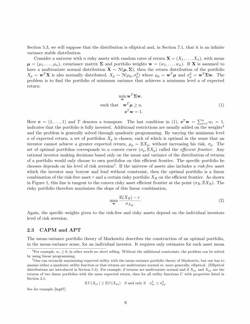
and the problem is generally solved through quadratic programming. By varying the minimum levela of expected return, a set of portfolios Xp is chosen, each of which is optimal in the sense that aninvestor cannot achieve a greater expected return, µp = EXp, without increasing his risk, σp. Theset of optimal portfolios corresponds to a convex curve (σp, EXp) called the efficient frontier. Anyrational investor making decisions based only on the mean and variance of the distribution of returnsof a portfolio would only choose to own portfolios on this efficient frontier. The specific portfolio hechooses depends on his level of risk aversion5. If the universe of assets also includes a risk-free assetwhich the investor may borrow and lend without constraint, then the optimal portfolio is a linearcombination of the risk-free asset r and a certain risky portfolio XR on the efficient frontier. As shownin Figure 1, this line is tangent to the convex risky asset efficient frontier at the point (σR, EXR). Therisky portfolio therefore maximizes the slope of this linear combination,

maxw

E(XR)− r

σXR

. (2)

Again, the specific weights given to the risk-free and risky assets depend on the individual investorslevel of risk aversion.

2.3 CAPM and APT

The mean-variance portfolio theory of Markowitz describes the construction of an optimal portfolio,in the mean-variance sense, for an individual investor. It requires only estimates for each asset mean

4For example, wi ≥ 0, in other words no short selling. Without the additional constraints, the problem can be solvedby using linear programming.

5One can reconcile maximizing expected utility with the mean-variance portfolio theory of Markowitz, but one has toassume either a quadratic utility function or that returns are multivariate normal or, more generally, elliptical. (Ellipticaldistributions are introduced in Section 5.3). For example, if returns are multivariate normal and if Xp1 and Xp2 are thereturns of two linear portfolios with the same expected return, then for all utility functions U with properties listed inSection 2.1,

E U(Xp1) ≥ E U(Xp2) if and only if σ2p1 ≤ σ2

p2 .

See for example [Ing87].

6

R

σ

µ

r

Figure 1: The efficient frontier (σp, µp). In the case when only risky assets R are available, the frontiertraces out a convex curve in risk-return space. The inclusion of a risk-free asset r, has a profoundeffect on the efficient set. In this case, all efficient portfolios will consist of linear combinations of rand some risky portfolio R, where (σR, µR) lies on the efficient frontier.

return, and the covariance between assets6. If all investors act in a way consistent with Markowitz’theory, then under additional assumptions, one will be able to learn something about the trade-offbetween risk and return in a market in equilibrium7. This is what the CAPM does.

The capital asset pricing model (CAPM) is an equilibrium pricing model (see Sharpe [Sha64] andLintner [Lin65]) which relates the expected return of an asset to the risk-free return, to the market’sexpected return and to the covariance between the market and the asset. In addition to assumingthat market participants use the mean-variance framework, the model makes two additional majorassumptions. First, the market is assumed frictionless. This means that securities are infinitelydivisible, there exist no transaction costs, no taxes, and there are no trading restrictions. Second, theinvestors beliefs are homogeneous. This means investors agree on mean returns and covariances for allassets in the market.

The efficient frontier in Figure 1 depended on the investors’ belief. Under the CAPM assumptions,since all investors assume the same expected return and covariances for all assets in the market, theyall have the same (risky) efficient frontier. However, the individual investors choice of the optimal riskyportfolio still depends on the investors own level of risk aversion. Additionally, with the inclusion of arisk-free asset, we saw that the investors portfolios become dramatically more simple. Each investorcan own only two assets: the risk-free asset and an optimal risky portfolio, with the relative weightsdepending on the investors appetite for risk. But since each investor holds the same optimal portfolio

6For a universe of n assets it is necessary to compute n(n − 1)/2 + n covariances. This means that if the universeunder consideration consists of n = 1000 assets, it is necessary to estimate over 500 000 covariances.

7By market equilibrium, we mean a market place where security prices are set so that supply equals demand.

7

of risky assets, and since the market is assumed to be in equilibrium, this optimal risky portfolio mustbe the market portfolio. Thus Figure 1 applies with R = M , where M denotes the market portfolio.M consists of all risky assets held in proportion to their overall market capitalization. Letting XM

denote the return on the market portfolio, Xi denote the return of asset i, and r denote the risk-freereturn, the CAPM establishes the following relationship:

E(Xi − r) = βiE(XM − r) (3)

whereβi =

Cov(Xi, XM )VarXM

. (4)

The CAPM thus relates in a linear way the expected premium EXi − r of holding the risky asset iover the risk-free asset to the expected premium EXM − r of holding the market portfolio over therisk-free asset. The constant of proportionality is the asset’s beta. The coefficient βi is a measure ofasset i’s sensitivity to the market portfolio. The expected premium for asset i is greater than that ofthe market if βi > 1 and less if βi < 1. But if βi > 1, then the risk will be greater. Indeed, if weassume that

Xi − r = βi(XM − r) + εi, (5)

where εi is such that Eεi = 0 and Cov(εi, XM ) = 0, then we have (3) and

σ2Xi

= β2i σ2

XM+ σ2

εi. (6)

Equation (5) is often known as a single factor model for asset returns. Notice from (6) that the asset’srisk is the sum of two terms, the systematic or market risk β2

i σ2XM

and the unsystematic or residualrisk σ2

εi. For a portfolio Xp with weights w = (w1, . . . , wn), one gets similarly σ2

Xp= β2

pσ2XM

+ σ2εp

where βp =∑n

i=1 wiβi. If one additionally assumes that Cov(εi, εj) = 0 for all i 6= j then the residualrisk is

σ2εp

=n∑

i=1

w2i σ

2εi. (7)

It is bounded by c/n for some constant c, if for example, wi = 1/n, and hence the portfolio’s residualrisk can be greatly reduced by diversification. The investor, for example, is only rewarded for bearingsystematic or market risk, that is, he can expect a higher return than the market only by holding aportfolio which is riskier (βp > 1) than the market.

In the CAPM, all assets are exposed to a single common source of randomness, namely the market.The arbitrage pricing theory (APT) model, due to Ross [Ros76], is a generalization of the CAPM inwhich assets are exposed to a larger number of common sources of randomness. The APT differs fromthe CAPM in that the mean-variance framework that led to (5) is now replaced by the assumption ofa multifactor model

Xi = αi + βi1f1 + · · ·+ βikfk + εi (8)

for generating security returns. All assets are exposed to the k sources of randomness fj , j = 1, . . . , k,called factors. Additionally, each asset i is exposed to its own specific source of randomness εi. Theequilibrium argument used in the CAPM led to the central result (3). In the APT, the equilibriumassumption takes a slightly different form, namely, one assumes that the market is free of arbitrage.

8

−5 0 50

0.1

0.2

0.3

0.4

0.5

0.6

−5 0 5−5

0

5

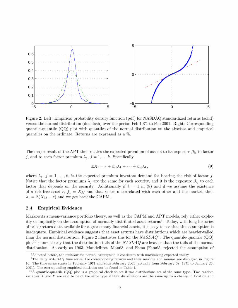
Figure 2: Left: Empirical probability density function (pdf) for NASDAQ standardized returns (solid)versus the normal distribution (dot-dash) over the period Feb 1971 to Feb 2001. Right: Correspondingquantile-quantile (QQ) plot with quantiles of the normal distribution on the abscissa and empiricalquantiles on the ordinate. Returns are expressed as a %.

The major result of the APT then relates the expected premium of asset i to its exposure βij to factorj, and to each factor premium λj , j = 1, . . . k. Specifically

EXi = r + βi1λ1 + · · ·+ βikλk, (9)

where λj , j = 1, . . . , k, is the expected premium investors demand for bearing the risk of factor j.Notice that the factor premiums λj are the same for each security, and it is the exposure βij to eachfactor that depends on the security. Additionally if k = 1 in (8) and if we assume the existenceof a risk-free asset r, f1 = XM and that εi are uncorrelated with each other and the market, thenλ1 = E(XM − r) and we get back the CAPM.

2.4 Empirical Evidence

Markowitz’s mean-variance portfolio theory, as well as the CAPM and APT models, rely either explic-itly or implicitly on the assumption of normally distributed asset returns8. Today, with long historiesof price/return data available for a great many financial assets, it is easy to see that this assumption isinadequate. Empirical evidence suggests that asset returns have distributions which are heavier-tailedthan the normal distribution. Figure 2 illustrates this for the NASDAQ9. The quantile-quantile (QQ)plot10 shows clearly that the distribution tails of the NASDAQ are heavier than the tails of the normaldistribution. As early as 1963, Mandelbrot [Man63] and Fama [Fam65] rejected the assumption of

8As noted before, the multivariate normal assumption is consistent with maximizing expected utility.9The daily NASDAQ time series, the corresponding returns and their maxima and minima are displayed in Figure

16. The time series starts in February 1971 and ends February 2001 (actually from February 08, 1971 to January 26,2001). The corresponding empirical statistics can be found in Table 1.

10A quantile-quantile (QQ) plot is a graphical check to see if two distributions are of the same type. Two randomvariables X and Y are said to be of the same type if their distributions are the same up to a change in location and

9

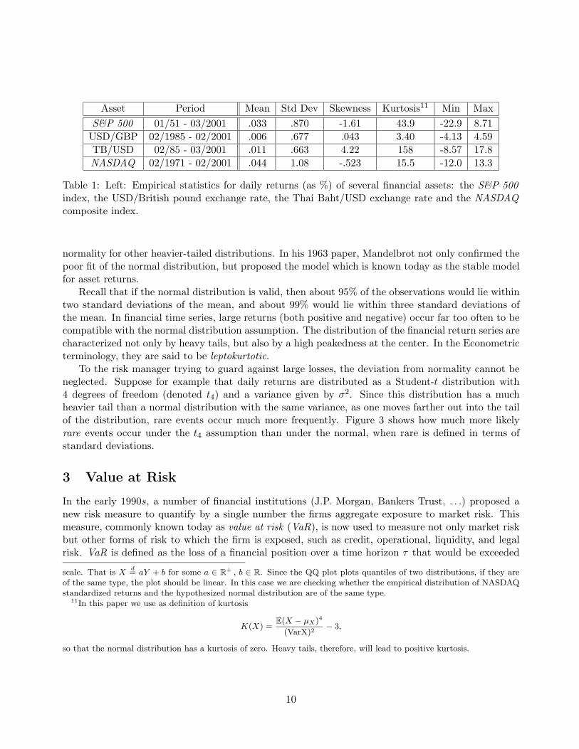
Asset Period Mean Std Dev Skewness Kurtosis11 Min MaxS&P 500 01/51 - 03/2001 .033 .870 -1.61 43.9 -22.9 8.71

USD/GBP 02/1985 - 02/2001 .006 .677 .043 3.40 -4.13 4.59TB/USD 02/85 - 03/2001 .011 .663 4.22 158 -8.57 17.8NASDAQ 02/1971 - 02/2001 .044 1.08 -.523 15.5 -12.0 13.3

Table 1: Left: Empirical statistics for daily returns (as %) of several financial assets: the S&P 500index, the USD/British pound exchange rate, the Thai Baht/USD exchange rate and the NASDAQcomposite index.

normality for other heavier-tailed distributions. In his 1963 paper, Mandelbrot not only confirmed thepoor fit of the normal distribution, but proposed the model which is known today as the stable modelfor asset returns.

Recall that if the normal distribution is valid, then about 95% of the observations would lie withintwo standard deviations of the mean, and about 99% would lie within three standard deviations ofthe mean. In financial time series, large returns (both positive and negative) occur far too often to becompatible with the normal distribution assumption. The distribution of the financial return series arecharacterized not only by heavy tails, but also by a high peakedness at the center. In the Econometricterminology, they are said to be leptokurtotic.

To the risk manager trying to guard against large losses, the deviation from normality cannot beneglected. Suppose for example that daily returns are distributed as a Student-t distribution with4 degrees of freedom (denoted t4) and a variance given by σ2. Since this distribution has a muchheavier tail than a normal distribution with the same variance, as one moves farther out into the tailof the distribution, rare events occur much more frequently. Figure 3 shows how much more likelyrare events occur under the t4 assumption than under the normal, when rare is defined in terms ofstandard deviations.

3 Value at Risk

In the early 1990s, a number of financial institutions (J.P. Morgan, Bankers Trust, . . .) proposed anew risk measure to quantify by a single number the firms aggregate exposure to market risk. Thismeasure, commonly known today as value at risk (VaR), is now used to measure not only market riskbut other forms of risk to which the firm is exposed, such as credit, operational, liquidity, and legalrisk. VaR is defined as the loss of a financial position over a time horizon τ that would be exceeded

scale. That is Xd= aY + b for some a ∈ R+ , b ∈ R. Since the QQ plot plots quantiles of two distributions, if they are

of the same type, the plot should be linear. In this case we are checking whether the empirical distribution of NASDAQstandardized returns and the hypothesized normal distribution are of the same type.

11In this paper we use as definition of kurtosis

K(X) =E(X − µX)4

(VarX)2− 3,

so that the normal distribution has a kurtosis of zero. Heavy tails, therefore, will lead to positive kurtosis.

10

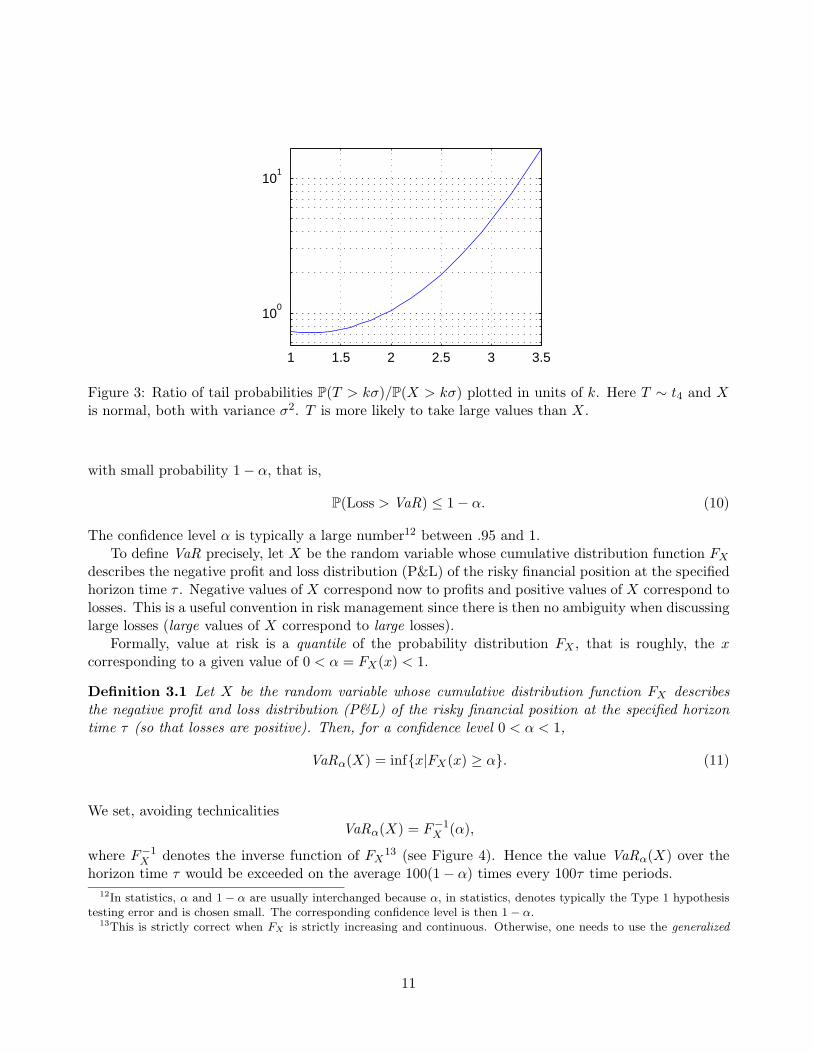
1 1.5 2 2.5 3 3.5

100

101

Figure 3: Ratio of tail probabilities P(T > kσ)/P(X > kσ) plotted in units of k. Here T ∼ t4 and Xis normal, both with variance σ2. T is more likely to take large values than X.

with small probability 1− α, that is,

P(Loss > VaR) ≤ 1− α. (10)

The confidence level α is typically a large number12 between .95 and 1.To define VaR precisely, let X be the random variable whose cumulative distribution function FX

describes the negative profit and loss distribution (P&L) of the risky financial position at the specifiedhorizon time τ . Negative values of X correspond now to profits and positive values of X correspond tolosses. This is a useful convention in risk management since there is then no ambiguity when discussinglarge losses (large values of X correspond to large losses).

Formally, value at risk is a quantile of the probability distribution FX , that is roughly, the xcorresponding to a given value of 0 < α = FX(x) < 1.

Definition 3.1 Let X be the random variable whose cumulative distribution function FX describesthe negative profit and loss distribution (P&L) of the risky financial position at the specified horizontime τ (so that losses are positive). Then, for a confidence level 0 < α < 1,

VaRα(X) = inf{x|FX(x) ≥ α}. (11)

We set, avoiding technicalitiesVaRα(X) = F−1

X (α),

where F−1X denotes the inverse function of FX

13 (see Figure 4). Hence the value VaRα(X) over thehorizon time τ would be exceeded on the average 100(1− α) times every 100τ time periods.

12In statistics, α and 1− α are usually interchanged because α, in statistics, denotes typically the Type 1 hypothesistesting error and is chosen small. The corresponding confidence level is then 1− α.

13This is strictly correct when FX is strictly increasing and continuous. Otherwise, one needs to use the generalized

11

VaRα

α

VaRα1

α1

VaRα2

α2

Figure 4: VaRα(X) for different cumulative distributions functions (cdfs) of the loss distribution X.The cdf on the right corresponds to an asset with discontinuous payoff, for example a binary option.See Definition 3.1.

Because of its intuitive appeal and simplicity, it is no surprise that VaR has become the de factostandard risk measure used around the world today. For example, today VaR is frequently used byregulators to determine minimum capital adequacy requirements. In 1995, the Basle Committee onBanking Supervision14 suggested that banks be allowed to use their own internal VaR models forthe purpose of determining minimum capital reserves. The internal models approach of the BasleCommittee is a ten day VaR at the α = 99% confidence level multiplied by a safety factor of at least3. Thus if VaR = 1M , the institution is required to have at least 3M in reserve in a safe account.

The safety factor of three is an effort by regulators to ensure the solvency of their institutions. Ithas also been argued, see Stahl [Sta97] or Danielsson, Hartmann and De Vries [DHV98] , that thesafety factor of three comes from the heavy-tailed nature of the return distribution. Since most VaRcalculations are based on the simplifying assumption that the distribution of returns are normal15,how bad does this assumption effect VaR? Assume that the Profit and Loss (P&L) distribution issymmetric and has finite variance σ2. Then regardless of the actual distribution, if X represents therandom loss over the specified horizon time with mean zero, Chebyshev’s inequality gives

P[X > cσ] ≤ 12c2

.

So if we are interested in VaR bounds for α = 0.99, setting 1/2c2 = 0.01 gives c = 7.071, and

inverse of FX , denoted F←X , and defined as

F←X (α) = inf{x |FX(x) ≥ α} , 0 < α < 1.

The definition (11) of VaRα(X) is then VaRα(X) = F←X (α). Thus, if FX(x) = α for x0 ≤ x ≤ x1, then VaRα(X) =F←X (α) = x0.

14See [oBS5a] and [oBS5b]. Basle is a city in Switzerland. In French, Basle is Bale, in German, it is Basel. Basle isthe old name for the city. The accent in Bale stands for the s that has been dropped from Basle.

15See for example the RiskMetrics manual [Met96].

12

this implies VaRmaxα=.99(X) = 7.071σ. If the VaR calculation were done under the assumption of

normality (Gaussian distribution) then VaRGaα=.99(X) = 2.326σ, and so if the true distribution is

indeed heavy-tailed with finite variance then the correction for VaRα=.99 of three is reasonable, since3× 2.326σ = 6.978σ.

3.1 Computation of VaR

Before we discuss how VaRα(X) is computed, we need to say a few words about X. Typically Xrepresents the risk of some aggregated position which is influenced by many underlying risk factorsY1, . . . , Yd,

X = f(Y1, . . . , Yd). (12)

The functional form of the dependence of X on the factors Y1, . . . , Yd is usually never known exactly,but it may be approximated in several standard ways depending on the nature of the position. Forexample, f is linear in the case of a portfolio of straight equity positions. The function f is non-linear,for example, if the portfolio contains a call option on an equity since the value of the call changesnon-linearly with respect to a change in the underlying asset. The usual procedure is to approximatethe change in the calls value with respect to its underlying by the options delta. For small changesin the underlying such an approximation is reasonable. However for large changes in the underlying,the approximation can be quite bad. In an effort to improve the approximation, a second orderterm is sometimes added, the options gamma. This second order approximation is referred to as thedelta-gamma approximation.

In practice, the VaR of a risky position X is calculated in one of three ways: through historicalsimulation, through a parametric model, or through some sort of Monte Carlo simulation. Eachway involves assumptions and approximations and it is the responsibility of the user to be aware ofthem. The risk manager who blindly performs the model calculations does so at his or her peril.For a full treatment of the commonly used procedures for the calculation of VaR, see Jorion [Jor01],Dowd [Dow98] or Wilson [Wil98]. See Duffie and Pan [DP97] for a discussion of heavy tails and VaRcalculations. We now describe the three ways of calculating VaR.

3.1.1 Historical Simulation VaR

The historical simulation model uses the historical returns of assets currently held in the portfolio inorder to calculate VaR16. First, returns over the horizon time τ are constructed for each asset in theportfolio using historical price information. Then portfolio returns are computed using the currentweight distribution of assets as though the portfolio had been held during the whole historical periodwhich is being sampled. The VaR is then read from the historical sample by using the order statistics.For example, if 1000 time periods are sampled, then 1000 portfolio returns are calculated, one for eachtime period. Let X

(1)p ≥ X

(2)p ≥ · · · ≥ X

(1000)p be the order statistics of these returns, where losses

are positive. Then VaRα=0.95(Xp) = X(50)p . The size of the sample is chosen by the user, but may be

constrained by the available data for some of the assets currently held.The model is simple to implement and has several advantages. Since it is based on historical prices

it allows for a nonlinear dependence between assets in the portfolio and underlying risk factors. Also16Over a fixed time horizon, VaR may be reported in units of rate of return (%) or of currency (profit and loss) since

these are essentially the same, up to multiplication by the initial wealth/value.

13

since it uses historical returns it allows for the presence of heavy tails without making assumptions onthe probability distributions of returns of the assets in the portfolio. There is therefore no model risk.In addition, there is no need to worry about the dependence structure of assets within the portfoliosince it is already reflected in the price and return data.

The drawbacks are typical of models involving historical data. There may not be enough dataavailable and there may be no reason to believe that the future will look like the past. For example, ifthe user would like to compute VaR for regulatory requirements, then τ = 10 days. With about 260business days, there are only 26 such observations in each year, four years worth of data are requiredto get about 100 historical simulations. This is the absolute minimum necessary to calculate VaRwith α = .99, since with 100 data points, there is but a single observation in the tail. If one or severalof the assets in the portfolio have insufficient histories then adjustments must be made. For example,some practitioners bootstrap from the shorter return histories in order to take advantage of the longerhistories on other assets.

When working only with historical data it is important to realize that we are assuming that thefuture will look like the past. If this assumption is likely to be unrealistic, the VaR estimate may bedangerously off the mark. For instance, if the sample period or window is devoid of large price changes,then our historical VaR will be low. But it will be large if there were large price fluctuations during thesample period. As large price fluctuations leave the sample window, the VaR will change accordingly.This yields a highly variable estimate and one which does not take into account the current financialclimate. The deficiencies of historical simulation notwithstanding, its ease of use makes it the mostpopular method for VaR calculations.

3.1.2 Parametric VaR

The parametric VaR model assumes that the returns possess a specific distribution, usually normal.The parameters of the distribution are estimated using either historical data or forward looking optiondata.

Example 3.1 Assume that over the desired time horizon τ the (negative) return distri-bution of a portfolio is given by FX ∼ N(µτ , σ

2τ ). Then the value at risk of portfolio X for

horizon τ and confidence level α > 0.5 is given by

VaRα(X) = inf{x|FX(x) ≥ α}= F−1

X (α)= µτ + στΦ−1(α),

where Φ−1(α) is the α quantile of the standard normal distribution.

More generally, if the (negative) return distribution of X is any FX with finite mean µτ and finitevariance σ2

τ , thenVaRα(X) = µτ + στqα, (13)

where qα is the α quantile of the standardized version of X. In other words, qα = F−1X

(α) whereX = (X − µτ )/στ .

If the VaR is computed under the assumption that returns are light-tailed, say normal, when infact they are heavy tailed, say tν (Student-t distribution with ν degrees of freedom), the risk may be

14

seriously underestimated for high confidence levels. This is because for large α, F−1normal(α) ≤ F−1

tν (α),so that the value of x that achieves Fnormal(x) = α is smaller than the value of x that achievesFtν (x) = α. It is thus very important that the return distribution be modelled well. A wide variety ofparametric distributions can be considered.

Within the portfolio context, the most easily implemented parametric model is the so called delta-normal method, where the joint distribution of the risk factor returns is multivariate normal and thereturns of the portfolio are assumed to be a linear function of the returns of the underlying risk factors.In this case the portfolio returns are themselves normally distributed.

Example 3.2 Take a portfolio of equities whose (negative) returns are given by Xp =w1X1 + . . . + wnXn where wi is the weight given to asset i and Xi is the assets (negative)return over the horizon in question. Assume (X1, . . . , Xn) ∼ N(0,Σ). Then, for α ∈(0.5, 1),

VaRα(Xp) = Φ−1(α)√

wTΣw

=√−−−→

VaRαT ρ−−−→VaRα,

where−−−→VaRα = (VaRα(w1X1), . . . ,VaRα(wnXn)) is the vector of the individual weighted

asset VaRs and ρ is the asset return correlation matrix. See Dowd [Dow98] for details.

When the number of assets is large, the central limit theorem is often invoked in defense of thenormal model. Even if the individual asset returns are non-normal, the central limit theorem tellsus that the weighted sum of many assets should be approximately normal. This argument may bedisposed of in various ways. Consider, for example, the empirical distribution of daily returns of alarge diversified index such as the NASDAQ , which is clearly heavy-tailed (see Figure 2). From aprobabilistic point of view it is not at all obvious that the assumptions of the central limit theoremare satisfied. For example, if the returns do not have finite variance, there may be convergence to theclass of stable distributions.

The class of stable distributions (also known as α-stable or stable Paretian) may be defined ina variety of ways. More will be said about them in Section 7. We define, at this stage, a stabledistribution as the only possible limiting distribution of appropriately normalized sums of independentrandom variables.

Definition 3.2 The random variable X has a stable distribution if there exists a sequences of i.i.d.random variables {Yi} and constants {an} ∈ R and {bn} ∈ R+ such that

Y1 + · · ·+ Yn

bn− an

d−→ X as n →∞. (14)

The stable distribution of X in (14) is characterized by four parameters (α, σ, β, µ) and we writeX ∼ Sα(β, σ, µ). The parameter α ∈ (0, 2] is called the index of stability or the tail exponent andcontrols the decay in the tails of the distribution. The remaining parameters σ, β, µ control scale,skewness, and location respectively. If the Yi have finite variance (the case in the usual CLT) thenα = 2 and the distribution of X is Gaussian. For all α ∈ (0, 2) the distribution is non-Gaussian stableand possess heavy tails.

15

Example 3.3 Properties of weekly returns of the Nikkei 225 Index over a 12 year periodare examined in Mittnik, Rachev and Paolella [MRP98]. The authors fit the return dis-tribution using a number of parametric distributions, including the normal, Student-t andstable. According to various measures of goodness of fit, the partially asymmetric Weibull,Student-t and the asymmetric stable provide the best fit. The fit by the normal is shownto be relatively poor. The stable distribution, in addition, fits best the tail quantiles of theempirical distribution, which is a result most relevant to the calculation of VaR.

The central limit theorem typically assumes independence. Although it has extensions to allowfor mild dependence, this dependence must be sufficiently weak. In fact, for a given number ofassets, the greater the dependence, the worse the normal approximation. This affects the speed of theconvergence. Since a VaR calculation involves the tails of the distribution, it is most important thatthe approximation hold in the tails. However, even when the conditions for the central limit theoremhold, the convergence in the tail is known to be very slow. The normal approximation may then onlybe valid in the central part of the distribution. In this case, the return distribution may be betterapproximated by a heavier-tailed distribution such as the Student-t or hyperbolic whose use in financeis becoming more common.

The hyperbolic distribution is a subclass of the class of generalized hyperbolic distributions. Thegeneralized hyperbolic distributions were introduced in 1977 by Barndorff-Neilsen [BN77] in order toexplain empirical findings in geology. Today these distributions are becoming popular in finance, andin particular in risk management. Two subclasses, the hyperbolic and the inverse Gaussian, are mostcommonly used. Both these subclasses may be shown to be mixtures of Gaussians. As such, theypossess heavier tails than the normal distribution but not as heavy as the stable distribution. For anintroduction to generalized hyperbolic distributions in finance, see for example Eberlein and Keller[EK95], Eberlein and Prause [EP00] or Shiryaev [Shi99].

3.1.3 Monte Carlo VaR

Monte Carlo procedures are perhaps the most flexible methods for computing VaR. The risk managerspecifies a model for the underlying risk factors, which incorporates somehow their dependence. Forexample, the risk factors in (12) may be described by the stochastic differential equation

dY(i)t = Y

(i)t (µ(i)

t dt + σ(i)t dW

(i)t ), (15)

for i = 1, . . . , d, where Wt = (W (1)t , . . . , W

(d)t ) is a multivariate Wiener process. Once parameters

of the model are estimated, for example by using historical data, or option implied estimates, therisk factors paths are then computer generated, thousands of paths for each risk factor. Each set ofsimulated paths for the risk factors yields a portfolio path and the portfolio is priced accordingly. Eachcomputed price of the portfolio represents a point on the portfolio’s return distribution. After manysuch points are obtained the portfolio’s VaR may then be read off the simulated distribution.

This method has the advantage of being extremely versatile. It allows for heavy tails, non-linearpayoffs and a great many other user specifications. Within the Monte Carlo framework, risk managersmay use their own pricing models to determine non-linear payoffs under many different scenarios forthe underlying risk factors. The method has also the advantage of allowing for time varying parameterswithin the risk factor processes. See for example Broadie and Glasserman [BG98].

16

There are two major drawbacks to Monte Carlo methods. First, they are computationally veryexpensive. Thousands of simulations of the risk factors may have to be carried out for results to betrusted. For a portfolio with a large number of assets this procedure may quickly become unmanage-able, since each asset within the portfolio must be valued using these simulations. Second, the methodis prone to model risk. The risk factors and the pricing models of assets with non-linear payoffs mayboth be mis-specified. And, as is the case of the parametric VaR, there is the risk of mis-specifyingthe model parameters.

3.2 Parameter Estimation

The parametric and Monte Carlo VaR methods require parameters to be estimated. When one is inter-ested in short time horizons, the primary goal is to estimate the volatility and covariance/correlation17.We outline some of the common estimation techniques here.

3.2.1 Historical Volatility

There are two different approaches to modelling volatility and covariance using only historical data.The more common approach gives constant weights to each data point. It assumes that volatility andcovariance are constant over time. The other approach attempts to address the fact that volatility andcovariance are time dependent by giving more weight to the more recent data points in the samplewindow.

First assume that variances and covariances do not to change over time. Take a large window oflength n in which historical data on the risk factors is available. Let Yi,tk be the return of factor i attime period tk. The variance of factor i and covariance of factors i and j are then computed by givingequal weights to each data point in the past. The n-period estimates at time T for the variance andcovariance

σ2i =

1n− 1

T−1∑t=T−n

(Yi,t − µYi)2 where µYi =

1n

T−1∑t=T−n

Yi,t (16)

and

σi,j =1

n− 1

T−1∑t=T−n

(Yi,t − µYi)(Yj,t − µYj ) (17)

respectively18. Since equal weight is given to each data point in the sample, the estimated volatilityand covariance change only slowly. If one keeps the window length fixed, the estimated values will riseor fall as new large returns enter the sample period and old large returns leave it. This means thateven a single extreme return will affect the estimates in the same way, whether it occurred at timeT − 1 or time T − n. The estimated variance and covariance, therefore, are greatly influenced by thechoice of the window size n.

Another stylized fact of financial time series, however, is that volatility itself is volatile. With thisin mind, another historical estimate of variance and covariance uses a weighting scheme which gives

17For example, over short time horizons, the mean return is usually assumed to be zero.18The normalization constant n− 1 gives an unbiased estimate. It is sometimes replaced by n in order to correspond

to the maximum likelihood estimate.

17

more weight to more recent observations. The corresponding estimates of variance and covariance are

σ2i (T ) =

T−1∑t=T−n

αt(Yi,t − µYi)2,

σi,j(T ) =T−1∑

t=T−n

αt(Yi,t − µYi)(Yj,t − µYj ),

where the weights αt,∑T−1

t=T−n αt = 1, are chosen to reflect current volatility conditions. In particular,more weight is given to recent observations: 1 > αT−1 > αT−2 > . . . > αT−n > 0. The model usingexponentially decreasing weights, such as that used by RiskMetrics, is probably the most popular. InRiskMetrics, the volatility estimator is given by

σi(T ) =

√√√√(1− λ)n∑

t=1

λt−1(Yi,T−t − µYi)2 (18)

where the decay factor λ is chosen to best match a large group of assets19. The covariance estimate issimilar. RiskMetrics choses λ = 0.94 in the case of daily returns.

The choice (18) allows the forecast of the next periods volatility given the current information,and hence to make parametric VaR calculations given the current information. To see this, assumethat the time T (negative) return distribution XT is being modelled by

XTd= σT ZT (19)

where Zt, t ∈ Z, is an innovation process, that is a sequence of i.i.d. mean zero and unit variancerandom variables. Letting Ft denote the filtration20 we have

σ2T+1|FT

= (1− λ)∞∑

t=0

λtX2i,T−t

= (1− λ)X2T + λ(1− λ)(X2

T−1 + λX2T−2 + λ2X2

T−3 + · · · )= (1− λ)X2

T + λσ2T |FT−1

.

This allows us to make our VaR calculation depend on the conditional return distribution FXT+1|FT.

If VaRT+1α (X) denotes the estimated value at risk for X at confidence level α for the period T + 1 at

time T , then, by (19),VaRT+1

α (X) = σT+1|FTqα,

19In this estimate it is assumed that the decay parameter λ and window length n are such that the approximation

n∑t=1

λt−1 ∼= 1

1− λ

is valid.20Conditioning over FT means conditioning over all the observations X1, . . . , XT .

18

1971 1974 1976 1979 1982 1984 1987 1990 1993 1995 1998

2

4

6

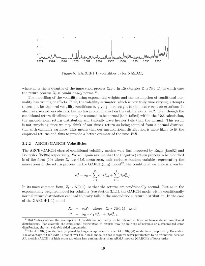
Figure 5: GARCH(1,1) volatilities σt for NASDAQ.

where qα is the α quantile of the innovation process Zt+1. In RiskMetrics Z is N(0, 1), in which casethe return process Xt is conditionally normal21.

The modelling of the volatility using exponential weights and the assumption of conditional nor-mality has two major effects. First, the volatility estimator, which is now truly time varying, attemptsto account for the local volatility conditions by giving more weight to the most recent observations. Italso has a second less obvious, but no less profound effect on the calculation of VaR. Even though theconditional return distribution may be assumed to be normal (thin-tailed) within the VaR calculation,the unconditional return distribution will typically have heavier tails than the normal. This resultis not surprising since we may think of our time t return as being sampled from a normal distribu-tion with changing variance. This means that our unconditional distribution is more likely to fit theempirical returns and thus to provide a better estimate of the true VaR.

3.2.2 ARCH/GARCH Volatilities

The ARCH/GARCH class of conditional volatility models were first proposed by Engle [Eng82] andBollerslev [Bol86] respectively. We will again assume that the (negative) return process to be modelledis of the form (19) where Zt are i.i.d. mean zero, unit variance random variables representing theinnovations of the return process. In the GARCH(p, q) model22, the conditional variance is given by

σ2t = α0 +

p∑i=1

αiX2t−i +

q∑j=1

βjσ2t−j .

In its most common form, Zt ∼ N(0, 1), so that the returns are conditionally normal. Just as in theexponentially weighted model for volatility (see Section 3.1.1), the GARCH model with a conditionallynormal return distribution can lead to heavy tails in the unconditional return distribution. In the caseof the GARCH(1, 1) model

Xt = σtZt where Zt ∼ N(0, 1) i.i.d.,σ2

t = α0 + α1X2t−1 + β1σ

2t−1,

21RiskMetrics allows the assumption of conditional normality to be relaxed in favor of heavier-tailed conditionaldistributions. For example the conditional distribution of returns may be mixture of normals or a generalized errordistribution, that is, a double sided exponential.

22The ARCH(p) model first proposed by Engle is equivalent to the GARCH(p, 0) model later proposed by Bollerslev.The advantage of the GARCH model over the ARCH model is that it requires fewer parameters to be estimated, becauseAR models (ARCH) of high order are often less parsimonious than ARMA models (GARCH) of lower order.

19

−4 −2 0 2 4−8

−6

−4

−2

0

2

4

Figure 6: Quantile-quantile (QQ) plot of the conditionally normal GARCH(1,1) standardized ex postinnovations for NASDAQ with the N(0, 1) distribution.

it is straightforward to show that under certain conditions23 the unconditional centered kurtosis isgiven by

K =EX4

t

(EX2t )2

− 3 =6α2

1

1− β21 − 2α1β1 − 3α2

1

,

which for most financial return series will be greater than zero. For example, in the case of a stationaryARCH(1) model, Xt =

√α0 + α1X2

t−1Zt, with α0 > 0 and α1 ∈ (0, 2eγ), where γ is Euler’s constant24,Embrechts, Kluppelberg and Mikosch [EKM97] show that the unconditional distribution is formallyheavy-tailed, that is

P(X > x) ∼ cx−α, x →∞. (20)

where α/2 > 0 is the unique solution to the equation h(u) = (2α1)u√π

Γ(u + 1

2

)= 1.

The ARCH/GARCH models allow for both volatility clustering (periods of large volatility) andfor heavy tails. The GARCH(1,1) estimated volatility process σt for the NASDAQ is displayed inFigure 5. The assumption of conditional normality can be checked, for example, by examining aQQ plot of the ex post innovations, that is Zt = Xt/σt. Figure 6 displays the QQ plot of Zt in thetraditional, conditionally normal GARCH(1,1) model for the NASDAQ . The fit of the GARCH(1,1)conditionally normal model in the lower tail is poor, showing the lower tail of Zt is heavier than thenormal distribution.

If the distribution of the historical innovations Zt−n, . . . , Zt is heavier-tailed than the normal,one can modify the model to allow a heavy-tailed conditional distribution FXt+1|Ft

25. In Panorska,23These conditions are α1 + β1 < 1 to guarantee stationarity, and 3α2

1 + 2α1β1 + β21 < 1 for K > 0. Both are generally

met in financial time series.24Euler’s constant γ is given by γ = limn→∞

(∑nk=1

1k− ln n

)and is approximately γ ≈ 0.577.

25For example the GARCH module in the statistical software package SPlus allows for three different non-Gaussianconditional distributions. As long as the user can estimate the GARCH parameters, usually through maximum likelihood,there are virtually no limits to the choice of the conditional distribution.

20

Mittnik and Rachev [PMR95] and Mittnik, Paolella and Rachev [MPR97], returns on the Nikkei indexare modelled using an ARMA-GARCH model of the form

Xt = a0 +r∑

i=1

aiXt−i + εt +s∑

j=1

bjεt−j (21)

(contrast with (19)), where εt = σtZt, with Zt an i.i.d. location zero, unit scale heavy-tailed randomvariable. The conditional distribution of the return series FXt|Ft−1

is given by the distribution typeof Zt. The ARMA structure in (21) is used to model the conditional mean E(Xt|Ft−1) of the returnseries Xt. The GARCH structure is imposed on the scale parameter26 σt through

σ2t = α0 +

p∑i=1

αiε2t−i +

q∑j=1

βjσ2t−j .

Several choices for the distribution of Zt are tested. In the case where Zt are realizations from a stabledistribution, the GARCH model used is

σt = α0 +p∑

i=1

αi|εt−i|+q∑

j=1

βjσt−j ,

and the index of stability exponent α for the stable distribution is constrained to be greater than one.Using several goodness of fit measures, the authors find that it is better to model the conditional

distribution of returns for the Nikkei than the unconditional distribution, since the unconditionaldistribution cannot capture the observed temporal dependencies of the return series27. Within thetested models for Zt, the partially asymmetric Weibull, the Student-t, and the asymmetric stable alloutperform the normal. In order to perform reliable value at risk calculations one must model the tailof the distribution Zt particularly well. The Anderson-Darling (AD) statistic can be used to measuregoodness of fit in the tails. Letting Femp(x) and Fhyp(x) denote the empirical and hypothesizedparametric distributions respectively, the AD statistic

AD = supx∈R

|Femp(x)− Fhyp(x)|√Fhyp(x)(1− Fhyp(x))

gives more weight to the tails of the distribution. Using this statistic, as well as others, the authorspropose the asymmetric stable distribution as the best of the tested models for performing VaRcalculations at high quantiles.

The class of ARCH/GARCH models have become increasingly popular for computing VaR. Themodelling of the conditional distribution has two immediate benefits. First, it allows for the predictedvolatility (or scaling) to use local information, i.e. it allows for volatility clustering. Second, sincevolatility is allowed to be volatile, the unconditional distribution will typically not be thin-tailed. Thisis true, as we have seen, even when the conditional distribution is normal.

There now exist many generalizations of the class of ARCH/GARCH models. Models such asEGARCH, HGARCH, AGARCH, and others, all attempt to use the local volatility structure to better

26In their model σt is to be interpreted as a scale parameter, not necessarily a volatility, since for some of thedistributional choices for Zt, the variance may not exist.

27The type of the conditional distribution is that of Zt, the unconditional distribution is that of Xt.

21

predict future volatility while trying to account for other observed phenomenon. See Bollerslev, Chouand Kroner [BCK92] for a review. The time series of returns {Xt}t∈Z in (19) is generally assumedto be stationary. In a recent paper, Mikosch and Starica [MS00] show that this assumption is notsupported, at least globally, by the S&P 500 from 1953 to 1990 and the DEM/USD foreign exchangerate from 1975 to 1982. The authors show that when using a GARCH model the parameters mustbe updated to account for changes of structure (changes in the unconditional variance) of the timeseries. A method for detecting these changes is also proposed. Additionally, they show that the longrange dependence behavior associated with the absolute return series, another of the so called stylizedfacts of financial time series, may only be an artifact of structural changes in the series, that is, tonon-stationarity.

Stochastic volatility models are not limited to the class of ARCH/GARCH models and their gen-eralizations. Other models may involve additional sources of randomness. For example, the model ofHull and White [HW87]

dYt = µYt + σtYtdW(1)t ,

dVt = νVt + ξVtdW(2)t ,

where σ2t = Vt and (W (1)

t , W(2)t ) is a bivariate Wiener process, introduces a second source of randomness

through the volatility. The two sources of randomness W(1)t and W

(2)t need not be uncorrelated. Again,

the introduction of a stochastic scaling generally leads to an unconditional return distribution whichis leptokurtotic. See Shiryaev [Shi99], for an introduction to stochastic volatility models in discreteand continuous time.

3.2.3 Implied Volatilities

The parametric VaR calculation requires a forecast of the volatility. All of the models examined so farhave used historical data. One may prefer to use a forward looking data set instead of historical datain the forecast of volatility, for example options data, which provide the market estimate of futurevolatility. To do so, one could use the implied volatility derived from the Black-Scholes model. In thismodel, European call options prices Ct = C(St, K, r, σ, T−t) are an increasing function of the volatilityσ. The stock price St at time t, the strike price K, the interest rate r and the time to expiration T − tare known at time t. Since σ is the only unknown parameter/variable, we may then use the observedmarket price Ct to solve for σ. This estimate of σ is commonly called the (Black-Scholes) impliedvolatility. The Black-Scholes model, however is imperfect. While σ should be constant, one typicallyobserves that σ depends on the time to expiration T − t and on the strike price K. For fixed T − t, theimplied volatility σ = σ(T − t, K) as a function of the strike price K is often convex, a phenomenonknown as the volatility smile. To obtain volatility estimates it is common to use at-the-money options,where St = K, since they are the most actively traded and hence are thought to provide the mostaccurate estimates.

3.2.4 Extreme Value Theory

Since VaR calculations are only concerned with the tails of a probability distribution, techniques fromExtreme Value Theory (EVT) may be particularly effective. Proponents of EVT have made compellingarguments for its use in calculating VaR and for risk management in general. We will discuss EVT inSection 6.

22

4 Risk Measures

We have considered two different measures of risk: standard deviation and value at risk. Standarddeviation, used by Markowitz and others, is still commonly used in portfolio theory today. The secondmeasure,VaR, is the standard measure used today by regulators and investment banks. We detailedsome of the computational issues surrounding these measures but have not discussed their validity.

It is easy to criticize standard deviation and value at risk. Even in Markowitz’s pioneering work onportfolio theory, the shortcomings of standard deviation as a risk measure were recognized. In [Mar59],an entire chapter is devoted to semi-variance28 as a potential alternative. In Artzner, Delbaen, Eberand Heath [ADEH97], for example, measures based on standard deviation are criticized based on theirinability to describe rare events and VaR is criticized because of its inability to aggregate risks in alogical manner. In two now famous papers [ADEH97] and [ADEH99] on financial risk, the authorspropose a set of properties any reasonable risk measure should satisfy. Any risk measure which satisfiesthese properties is called coherent. We shall now introduce these properties and indicate why the riskmeasures described above are not coherent.

4.1 Coherent Risk Measures

Suppose that the financial position of an investor will lead at time T to a loss X29, which is a randomvariable. Let G be the set of all such X. A risk measure ρ is defined as a mapping from G to R.Intuitively, for a given potential loss X in the future we may think of ρ(X) as the minimum amountof cash that we need to invest prudently today (in a reference instrument) to be allowed to take theposition X30. A risk measure ρ may be coherent or not.

Definition 4.1 Given a reference instrument with return r, possibly random, a risk measure ρ satis-fying the following four axioms is said to be coherent:

Translation Invariance. For all X ∈ G and all α ∈ R, we have ρ(X + αr) = ρ(X) + α. This meansthat adding the amount α to the position, and investing it prudently, reduces the overall risk ofthe position by α.

Subadditivity. For all X1 and X2 ∈ G, ρ(X1 +X2) ≤ ρ(X1)+ρ(X2). Hence a merger does not createextra risk. This is the basis for diversification.

Positive Homogeneity. For all λ ≥ 0 and all X ∈ G, ρ(λX) = λρ(X). This requires that the riskscales with the size of a position. If the size of a position renders it illiquid, then this should beconsidered when modelling the future net worth.

Monotonicity. For all X and Y ∈ G with X ≥ Y , we have ρ(X) ≥ ρ(Y ). If the future net loss X isgreater, then X is more risky.

28In order to put the accent on (negative) returns above the mean, semi-variance is defined as

σX = E[(X − EX)1{X>EX}]2.

29Losses are positive and profits negative. This is at odds with the authors’ original notation.30The authors refer to X as risk and axiomatically define acceptance sets, which are sets of acceptable risks, and

proceed to define measures of risk as describing the risks proximity to the acceptance set.

23

The term coherent measure of risk has found its way into the risk management vernacular. It isdefined, for example, in the second edition of Philippe Jorion’s Value at Risk ([Jor01]).

Note that the axioms of translation invariance and monotonicity rule out standard deviation asa coherent measure of risk. Indeed, since σX+αr = σX , translation invariance fails, and since σ alsopenalizes the investor for large profits as well as large losses, monotonicity fails as well. Consider, forexample, two portfolios X and Y which are identical except for the free lottery ticket held in Y . Wehave X ≥ Y , since there is no down-side to the free ticket and therefore the potential losses in Y aresmaller than in X. Nevertheless, the standard deviation measure assigns to Y a higher risk, hencemonotonicity fails. Markowitz’s alternative risk measure semi-variance is not coherent either becauseit is not subadditive.

4.2 Expected Shortfall

VaR is not a coherent measure of risk because it fails to be subadditive in general. One can indeedeasily construct scenarios (see Albanese [Alb97]) where for two positions X and Y it is true that

VaRα(X + Y ) > VaRα(X) + VaRα(Y ).

This is contrary to the risk managers feelings, that the overall risk of different trading desks is boundedby the sum of their individual risks. In short, VaR fails to aggregate risks in a logical manner. Inaddition, VaR tells us nothing about the size of the loss that exceeds it. Two distributions may havethe same VaR yet be dramatically different in the tail.

Hence neither the standard deviation nor VaR are coherent. On the other hand, the expectedshortfall, also called tail conditional expectation, is a coherent risk measure. Intuitively, the expectedshortfall addresses the question: given that we will have a bad day, how bad do we expect it to be?It is a more conservative measure than VaR and looks at the average of all losses that exceed VaR.Formally, the expected shortfall for risk X and high confidence level α is defined as follows:

Definition 4.2 Let X be the random variable whose distribution function FX describes the negativeprofit and loss distribution (P&L) of the risky financial position at the specified horizon time τ (thuslosses are positive). Then the expected shortfall for X is

Sα(X) = E(X|X > VaRα(X)). (22)

Suppose, for example, that a portfolio’s risk is to be calculated through simulation. If 1000simulations are run, then for α = 0.95, the portfolios VaR would be the smallest of the 50 largestlosses. The corresponding expected shortfall would be estimated by the numerical average of these50 largest losses. Expected shortfall, therefore, tells us something about the expected size of a lossexceeding VaR. It is subadditive, coherent and puts fewer restrictions on the distribution of X,requiring only a finite first moment to be well defined. Additionally, it may be reconciled with theidea of maximizing expected utility. Levy and Kroll [LK78] show that for all utility functions U withthe properties described in Section 2.1 and all random variables X and Y (representing losses) that

E U(−X) ≥ E U(−Y ) ⇐⇒ Sα(X) ≤ Sα(Y ) for all α ∈ (0, 1).

Expected shortfall can be used in portfolio theory as a replacement of the standard deviation ifthe distribution of X is normal, or more generally, elliptical. As we will see in Section 5.3, in this

24

case any positive homogeneous translation invariant risk measure will yield the same optimal linearportfolio for the same level of expected return.

Unlike standard deviation, expected shortfall, as defined in (22), does not measure deviation fromthe mean. Bertsimas, Lauprete and Samarov [BLS00] define shortfall31 as

sα(X) = E(X |X > VaRα(X))− EX. (23)

The subtraction of the mean makes it more similar to the standard deviation σX =√

E(X − EX)2

and again, as far as portfolio theory is concerned, in the case of elliptical distributions, one obtains thesame optimal portfolio for the same level of expected return if one uses sα to measure risk. In fact, itcan be shown that for a linear portfolio Xp = w1X1 + · · ·+wnXn of multivariate normally distributedreturns X ∼ N(µ,Σ), that

sα(Xp) =φ(Φ−1(α))

1− ασp,

where φ(x) and Φ(x) are respectively, the pdf and cdf of a standard normal random variable evaluatedat x. In other words,

arg minAw=b

wTΣw = arg minAw=b

sα(wT X),

for all α ∈ (0, 1), where Aw = b is any set of linear constraints, including constraints that do notrequire all portfolios to have the same mean. Note, however, that sα is not coherent since it violatesthe axioms of translation invariance and monotonicity.

5 Portfolios and Dependence

The measure of dependence most popular in the financial community is linear correlation32. Its popu-larity may be traced back to Markowitz’ mean variance portfolio theory since, under the assumption ofmultivariate normality, the correlation is the canonical measure of dependence. Outside of the worldof multivariate normal distributions, correlation as a measure of dependence may lead to misleadingconclusions (see Section 5.2.1)33. The linear correlation between two random variables X and Y ,defined by

ρ(X, Y ) =Cov(X, Y )

σXσY, (24)

is a measure of linear dependence between X and Y . The word linear is used because when variancesare finite, ρ(X, Y ) = ±1 if and only if Y is an affine transformation of X almost surely, that isif Y = aX + b a.s. for some constants a ∈ R\{0}, and b ∈ R. When the distribution of returnsX is multivariate normal, the dependence structure of the returns is determined completely by thecovariance matrix Σ or, equivalently, by the correlation matrix ρ. One has Σ = [σ] ρ [σ] where [σ] isa diagonal matrix with the standard deviations σj on the diagonal.

When returns are not multivariate normal, linear correlation may no longer be a meaningful mea-sure of dependence. To deal with potential alternatives, we will introduce the concept of copulas,describe various measures of dependence and focus on elliptical distributions. For additional details

31We still assume losses are positive. This is at odds with the authors notation.32Also known as Pearson’s correlation.33Linear correlation is actually the canonical measure of dependence for the class of elliptical distributions. This class

will be introduced shortly and may be thought of as an extension of multivariate normal distributions.

25

and proofs, see Embrechts, McNeil and Straumann [EMS01], Lindskog [Lin00b], Nelsen [Nel99], Joe[Joe97] and Fang, Kotz and Ng [FKN90].

5.1 Copulas

When X = (X1, . . . , Xn) ∼ N(µ,Σ), the distribution of any linear portfolio of the Xj ’s is normal withknown mean and variance. In the non-normal case, the joint distribution of X,

F (x1, . . . , xn) = P(X1 ≤ x1, . . . , Xn ≤ xn)

is not fully described by its mean and covariance. One would like, however, to describe the joint distri-bution by specifying separately the marginal distributions, that is, the distribution of the componentsX1, . . . , Xn, and the dependence structure. One can do this with copulas.

Definition 5.1 An n-Copula is any function C : [0, 1]n → [0, 1] satisfying the following properties:

1. For every u = (u1, . . . , un) in [0, 1]n we have that C(u) = 0 if at least one component uj = 0and C(u) = uj if u = (1, . . . , 1, uj , 1, . . . , 1).

2. For every a, b ∈ [0, 1]n such that a ≤ b

2∑i1=1

· · ·2∑

in=1

(−1)i1+···inC(u1i1 , . . . , unin) ≥ 0 (25)

where uj1 = aj and uj2 = bj for j = 1, . . . , n.

Corollary 5.1 below provides a concrete way to construct copulas. It is based on the following theoremdue to Sklar (see [Skl96], [Nel99]), which states that by using copulas one can separate the dependencestructure of the multivariate distribution from the marginal behavior.

Theorem 5.1 (Sklar) Let F be an n-dimensional distribution function with marginals Xj ∼ Fj forj = 1, . . . , n. Then there exists an n-copula C : [0, 1]n → [0, 1] such that for every x = (x1, . . . , xn) ∈Rn,

F (x1, . . . , xn) = C(F1(x1), . . . , Fn(xn)). (26)

Furthermore, if the Fj are continuous then C is unique. Conversely, if C is an n-copula and Fj aredistribution functions, then F in (26) is an n-dimensional distribution function with marginals Fj.

The function C is called the copula of the multivariate distribution of X. Assuming continuity of themarginals Fj , j = 1, . . . , n, we see that the copula C of F is the joint distribution of the uniformtransformed variables Fj(Xj),

C(u1, . . . , un) = F (F−11 (u1), . . . , F−1

n (un)). (27)

Corollary 5.1 If the Fj are the cdfs of U(0, 1) random variables, then xj = Fj(xj), 0 < xj < 1,and (26) becomes F (x1, . . . , xn) = C(x1, . . . , xn). Therefore the copula C may be thought of as thecumulative distribution function (cdf) of a random vector with uniform marginals.

26

Copulas allow us to model the joint distribution of X in two natural steps. First, one models theunivariate marginals Xj . Second, one chooses a copula that characterizes the dependence structure ofthe joint distribution. Any n-dimensional distribution function can serve as a copula. The followingexamples relate familiar multivariate distributions to their associated copulas and marginals.

Example 5.1 Suppose X1, . . . , Xn are independent then

F (x1, . . . , xn) = P(X1 ≤ x1, . . . , Xn ≤ xn)= P(X1 ≤ x1) · · ·P(Xn ≤ xn)= F1(x1) · · ·Fn(xn).

Hence, in the case of independence, C(u1, . . . , un) = u1 · · ·un for all (u1, . . . , un) ∈ [0, 1]n.

Example 5.2 Suppose (X1, . . . , Xn) is multivariate standard normal with linear correla-tion matrix ρ. Let Φ(z) = P(Z ≤ z) for Z ∼ N(0, 1). Then

F (x1, . . . , xn) = P(X1 ≤ x1, . . . , Xn ≤ xn)= P(F1(X1) ≤ F1(x1), . . . , Fn(Xn) ≤ Fn(xn))= CGa

ρ (Φ(x1), . . . ,Φ(xn)),

where

CGaρ (u1, . . . , un) =

1√|ρ|(2π)n

∫ Φ−1(u1)

−∞· · ·

∫ Φ−1(un)

−∞e−

12sT ρ−1s ds (28)

is called the multivariate Gaussian copula.

Example 5.3 Suppose (X1, . . . , Xn) is multivariate t with ν degrees of freedom and linearcorrelation matrix ρ 34. Let tν(x) = P(T ≤ x) where T ∼ tν . Then

F (x1, . . . , xn) = P(X1 ≤ x1, . . . , Xn ≤ xn)= P(F1(X1) ≤ F1(x1), . . . , Fn(Xn) ≤ Fn(xn))= Ctν

ρ (tν(x1), . . . , tν(xn))

where

Ctνρ (u1, . . . , un) =

Γ(ν+n2 )

Γ(ν2 )

√|ρ|(νπ)n

∫ t−1ν (u1)

−∞· · ·

∫ t−1ν (un)

−∞

(1 +

sT ρ−1sν

)− ν+n2

ds (29)

is called the multivariate tν copula.

In Examples 5.2 and 5.3, |ρ| denotes the determinant of the matrix ρ. In these examples, the copulaswere introduced through the joint distribution, but it is important to remember that the copulacharacterizes the dependence structure of the multivariate distribution through (26). The Gaussianand tν copulas (28) and (29) exist separately from their associated multivariate distributions.

34Its cdf is given by (29) where the upper limits t−1ν (u1), . . . , t

−1ν (un) are replaced by x1, . . . , xn respectively. A

multivariate tν is easy to generate. Generate a multivariate normal with covariance matrix Σ and divide it by√

χ2ν/ν

where χ2ν is an independent chi-squared random variable with ν degrees of freedom.

27

Example 5.4 The bivariate Gumbel copula CGuβ is given by

CGuβ (u1, u2) = exp

{−

[(− lnu1)

1β + (− lnu2)

1β

]β}

, (30)

where 0 < β ≤ 1 is a parameter controlling the dependence, β → 0+ implies perfectdependence (see Section 5.2.3), and β = 1 implies independence.

Example 5.5 The bivariate Clayton copula CClβ is given by

CClβ (u1, u2) = (u−β

1 + u−β2 − 1)−

1β , (31)

where 0 < β < ∞ is a parameter controlling the dependence, β → 0+ implies independence,and β → ∞ implies perfect dependence. This copula family is sometimes referred to asthe Kimeldorf and Sampson family.

Both the Gumbel and Clayton copulas are strict Archimedian copulas. Archimedean copulas aredefined as follows. Let φ : [0, 1] → [0,∞) with φ(0) = ∞ and φ(1) = 0 be a continuous, convex, strictlydecreasing function. The transformation φ−1φ maintains the uniform 1-dimensional distribution sinceφ−1φ(u) = u, u ∈ [0, 1]. To obtain a 2-dimensional distribution function use instead of φ−1φ(u), u ∈[0, 1] the function φ−1(φ(u) + φ(v)), u, v ∈ [0, 1].

Definition 5.2 A strict Archimedian copula with generator φ is of the form

C(u, v) = φ−1(φ(u) + φ(v)), u, v ∈ [0, 1]. (32)

Example 5.6 The function φ(t) = (− ln t)1/β , 0 < β ≤ 1 generates the bivariate Gumbelcopula CGu

β (see Example 5.4).

Example 5.7 The function φ(t) = (t−β − 1)/β, β > 0 generates the bivariate Claytoncopula CCl

β (see Example 5.5).

Example 5.8 The function φ(t) = − ln((e−βt − 1)/(e−β − 1)), β ∈ R\{0} generates thebivariate Frank copula

CFrβ (u, v) = − 1

βln

(1 +

(e−βu − 1

) (e−βv − 1

)e−β − 1

)

(see Frank [Fra79]).

If φ(0) < ∞, then the term strict in Definition 5.2 is dropped and φ−1(s) in (32) is replaced by thepseudo-inverse φ[−1](s) which equals φ−1(s) if 0 ≤ s ≤ φ(0) and is zero otherwise.

Example 5.9 The function φ(t) = 1− t, t ∈ [0, 1] satisfies φ(0) = 1 and hence φ[−1](t) =max(1− t, 0). It generates the non-strict Archimedean copula

C(u, v) = max(u + v − 1, 0).

28

−3 −2 −1 0 1 2 3−3

−2

−1

0

1

2

3

−3 −2 −1 0 1 2 3−3

−2

−1

0

1

2

3

−3 −2 −1 0 1 2 3−3

−2

−1

0

1

2

3

−3 −2 −1 0 1 2 3−3

−2

−1

0

1

2

3

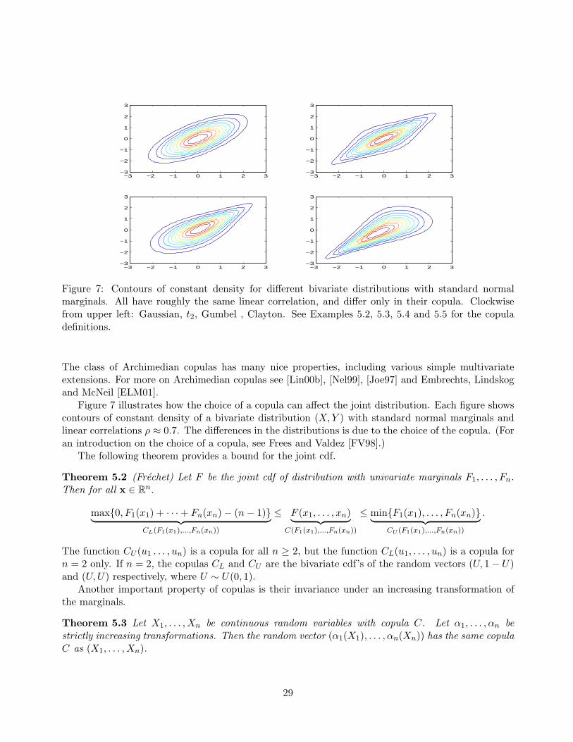
Figure 7: Contours of constant density for different bivariate distributions with standard normalmarginals. All have roughly the same linear correlation, and differ only in their copula. Clockwisefrom upper left: Gaussian, t2, Gumbel , Clayton. See Examples 5.2, 5.3, 5.4 and 5.5 for the copuladefinitions.

The class of Archimedian copulas has many nice properties, including various simple multivariateextensions. For more on Archimedian copulas see [Lin00b], [Nel99], [Joe97] and Embrechts, Lindskogand McNeil [ELM01].

Figure 7 illustrates how the choice of a copula can affect the joint distribution. Each figure showscontours of constant density of a bivariate distribution (X, Y ) with standard normal marginals andlinear correlations ρ ≈ 0.7. The differences in the distributions is due to the choice of the copula. (Foran introduction on the choice of a copula, see Frees and Valdez [FV98].)

The following theorem provides a bound for the joint cdf.

Theorem 5.2 (Frechet) Let F be the joint cdf of distribution with univariate marginals F1, . . . , Fn.Then for all x ∈ Rn.

max{0, F1(x1) + · · ·+ Fn(xn)− (n− 1)}︸ ︷︷ ︸CL(F1(x1),...,Fn(xn))

≤ F (x1, . . . , xn)︸ ︷︷ ︸C(F1(x1),...,Fn(xn))

≤ min{F1(x1), . . . , Fn(xn)}︸ ︷︷ ︸CU (F1(x1),...,Fn(xn))

.

The function CU (u1 . . . , un) is a copula for all n ≥ 2, but the function CL(u1, . . . , un) is a copula forn = 2 only. If n = 2, the copulas CL and CU are the bivariate cdf’s of the random vectors (U, 1− U)and (U, U) respectively, where U ∼ U(0, 1).

Another important property of copulas is their invariance under an increasing transformation ofthe marginals.

Theorem 5.3 Let X1, . . . , Xn be continuous random variables with copula C. Let α1, . . . , αn bestrictly increasing transformations. Then the random vector (α1(X1), . . . , αn(Xn)) has the same copulaC as (X1, . . . , Xn).

29

−5 0 5−5

0

5

−5 0 5−5

0

5

Figure 8: Simulation of 10000 realizations from bivariate distributions both with standard normalmarginals and linear correlation of ρ ≈ 0.7. The distribution on the left has a Gaussian copula, on theright a Gumbel copula. Compare the shapes with those illustrated in Figure 7, where the populationdistribution is used.

5.2 Measures of Dependence

As already mentioned, linear correlation is the only measure of dependence involved in the mean-variance portfolio theory. This theory assumes, either implicitly or explicitly, that returns are multi-variate normal. This assumption seems implausible today given the many complex financial productsin the marketplace and the empirical evidence against normality. Without the restrictive assumptionof normality, is linear correlation still an appropriate measure of dependence?

Linear correlation is often used in the financial community to describe any form of dependence.As illustrated in [EMS01] and Embrechts, McNeil and Straumann [EMS99], linear correlation is oftena very misunderstood measure of dependence. Consider the following example.

Example 5.10 Figure 8 represent 10000 simulations from bivariate distributions (X, Y )L

and (X, Y )R. In both cases X and Y have a standard normal distribution with (approxi-mately) the same linear correlation ρ ≈ 0.7. Thus, on the basis of the marginal distributionsand linear correlation, the two distributions are indistinguishable. The two distributionsare however clearly different. If positive values represent losses, the distribution on theright is clearly of greater concern to the risk manager since large losses in X and Y occursimultaneously. The two distributions differ only in their copula.

In the figure on the left the dependence structure is given by the bivariate Gaussian copula.Since the marginals are standard normal, this means that distribution is the bivariatestandard normal distribution with the given correlation coefficient. The copula in thefigure on the right the Gumbel copula given in (30) with β = 1/2. Various values of β weretried until the simulation sample linear correlation was ρ ≈ 0.7.

We now briefly describe several measures of dependence which may be useful to the risk manager.Again the reader in encouraged to look at the above references, especially [EMS01] for details.

30

5.2.1 Linear Correlation

The linear correlation coefficient ρ, defined in (24), is a commonly misused measure of dependence.To illustrate the confusion involved in interpreting it, consider the following classic example. LetX ∼ N(µ, σ2) and let Y = X2. Then ρ(X, Y ) = 0, yet clearly X and Y are dependent. Unless we arewilling to make certain assumptions about the multivariate distribution, linear correlation can thereforebe a misleading measure of dependence. Since the copula of a multivariate distribution describes itsdependence structure we would like to use measures of dependence which are copula-based. Linearcorrelation is not such a measure.

5.2.2 Rank Correlation

Two well-known rank correlation measures which are copula based and have better properties thanlinear correlation are the Kendall’s tau and Spearman’s rho.

Definition 5.3 Let (X1, Y1) and (X2, Y2) be two independent copies of (X, Y ). Then Kendall’s tau,denoted ρτ , is given by

ρτ (X, Y ) = P [(X1 −X2)(Y1 − Y2) > 0]− P[(X1 −X2)(Y1 − Y2) < 0] .

If the marginal distributions FX and FY of X and Y are continuous and if F is the bivariate distributionfunction of (X, Y ) with copula C, then ρτ can be expressed in terms of C as follows (see [EMS01]):

ρτ (X, Y ) = 4∫ 1

0

∫ 1

0C(u, v) dC(u, v)− 1.

Definition 5.4 Let X ∼ FX and Y ∼ FY . Spearman’s correlation, denoted ρS, is the linear correla-tion of FX(X) and FY (Y ), that is,

ρS(X, Y ) = ρ(FX(X), FY (Y )).

Spearman’s correlation can also be expressed in a form similar to Definition 5.3 (see [Lin00b]). Let(X1, Y1), (X2, Y2) and (X3, Y3) be three independent copies of (X, Y ). Then

ρS(X, Y ) = 3 (P [(X1 −X2)(Y1 − Y3) > 0]− P [(X1 −X2)(Y1 − Y3) < 0]) .

If the marginal distributions are continuous, ρS is related to the copula of the joint distribution asfollows:

ρS(X, Y ) = 12∫ 1

0

∫ 1

0C(u, v) du dv − 3.

Whereas linear correlation is a measure of linear dependence, both Kendall’s tau and Spearman’srho are measures of monotonic dependence. Since they are copula based, they are invariant understrictly increasing transformations35. Indeed, if α1, α2 are strictly increasing transformations, then

ρτ (α1(X1), α2(X2)) = ρτ (X1, X2),ρS(α1(X1), α2(X2)) = ρS(X1, X2),

but ρ(α1(X1), α2(X2)) 6= ρ(X1, X2).35Recall that invariance under increasing transformations is a property of copulas.

31

5.2.3 Comonotonicity

An additional important property of these rank correlations is their handling of perfect dependence.By perfect dependence we mean intuitively that X and Y are monotone functions of the same sourceof randomness. Recall that in the bivariate case, the Frechet bounds CL and CU in Theorem 5.2 arethemselves copulas. The following theorem shows that if the copula is CL or CU then X and Y areperfectly dependent.

Theorem 5.4 ([EMS01]). Suppose that the copula C of (X, Y ) is either CL or CU . Then there existmonotone functions α and β and a random variable Z such that

(X, Y ) d= (α(Z), β(Z)).

If C = CL then α and β are increasing and decreasing respectively. If C = CU , then both α and β areincreasing.

X and Y are said to be countermonotonic if they have copula CL. If they have copula CU , theyare said to be comonotonic. In fact, when FX and FY are continuous,

C = CL ⇐⇒ Y = T (X) a.s., T = F−1Y ◦ (1− FX) ↘,

C = CU ⇐⇒ Y = T (X) a.s., T = F−1Y ◦ FX ↗ .

Kendall’s tau and Spearman’s rho handle perfect dependence in a reasonable manner. Indeed,

Theorem 5.5 ([EMS01]). Let (X, Y ) ∼ F with continuous marginals and copula C. Then

ρτ (X, Y ) = −1 ⇐⇒ ρS(X, Y ) = −1 ⇐⇒ C = CL ⇐⇒ X and Y are countermonotonic,ρτ (X, Y ) = 1 ⇐⇒ ρS(X, Y ) = 1 ⇐⇒ C = CU ⇐⇒ X and Y are comonotonic.

The following theorem due to Hoffding and Frechet deals with linear correlation. See [EMS01] for itsproof.

Theorem 5.6 Let (X, Y ) be a random vector with marginals non-degenerate FX and FY and unspec-ified dependence structure. If X and Y have finite variance, then

1. The set of possible linear correlations is a closed interval [ρmin, ρmax] with ρmin < 0 < ρmax.

2. The extremal linear correlation ρ = ρmin is attained iff X and Y are countermonotonic; ρ = ρmax

is attained iff X and Y are comonotonic.

3. ρmin = −1 ⇐⇒ X and − Y are of the same type36; ρmax = 1 ⇐⇒ X and Y are of the sametype.

The following example shows that linear correlation does not handle perfect dependence in a reasonablemanner.

36Recall that two random variables are the same type if their distributions are the same up to a change in locationand scale.

32

0 1 2 3 4 5

−0.5

0

0.5

1

Figure 9: Range of maximal and minimal linear correlation in Example 5.11. The x-axis is in units ofσ. As σ increases, both the maximal and minimal linear correlations tend to zero.

Example 5.11 ([EMS01]). Let X ∼ Lognormal(0, 1) and Y ∼ Lognormal(0, σ2) withσ > 0. By Theorem 5.6, ρ = ρmin and ρ = ρmax when X and Y are countermonotonic andcomonotonic respectively. By Theorem 5.4, (X, Y ) d= (α(Z), β(Z)), and in fact, (X, Y ) d=(eZ , e−σZ) when X and Y are countermonotonic and (X, Y ) d= (eZ , eσZ) when X and Yare comonotonic, where Z ∼ N(0, 1). Hence ρmin = ρ(eZ , e−σZ) and ρmax = ρ(eZ , eσZ)where Z ∼ N(0, 1). Using the properties of the lognormal distribution, these maximal andminimal correlations can be evaluated explicitly and one gets

ρmin =e−σ − 1√

(e− 1)(eσ2 − 1), ρmax =

eσ − 1√(e− 1)(eσ2 − 1)

.

As σ increases, the maximal and minimal linear correlation both tend to zero even thoughX and Y are monotonic functions of the same source of randomness. This is illustrated inFigure 9.

5.2.4 Tail Dependence

There is a saying in finance that in times of stress all correlations go to one37. While it shows that thefinancial community uses linear correlation to describe any measure of dependence, it can also serveas motivation for the next measure of dependence, known as tail dependence.

Bivariate tail dependence measures the amount of dependence in the upper and lower quadranttail of the distribution. This is of great interest to the risk manager trying to guard against concurrentbad events in the tails.

37See [CPB00] for example.

33

Definition 5.5 Let X ∼ FX and Y ∼ FY and observe that as α → 1−, F−1X (α) →∞ and F−1

Y (α) →∞. The coefficient of upper tail dependence λU is

λU (X, Y ) = limα→1−

P(Y > F−1Y (α)|X > F−1

X (α)) (33)

provided the limit exists. If λU = 0, then X and Y are said to asymptotically independent in the uppertail. If λU ∈ (0, 1], then X and Y are asymptotically dependent in the upper tail. The coefficient oflower tail dependence λL is similarly defined:

λL(X, Y ) = limα→0+

P(Y < F−1Y (α)|X < F−1

X (α)).

Since

λU (X, Y ) = limα→1−

1− P(X ≤ F−1X (α))− P(Y ≤ F−1

Y (α)) + P(X ≤ F−1X (α), Y ≤ F−1

Y (α))1− P(X ≤ F−1

X (α)),

λU , as well as λL, can be expressed in terms of copulas. Let (X, Y ) have continuous distribution Fwith copula C. It is easily seen that the coefficient of upper tail dependence λU can be expressed as

λU (X, Y ) = limα→1−

C(α, α)1− α

, (34)

where C(α, α) = 1− 2α + C(α, α) 38. Similarly,

λL(X, Y ) = limα→0+

C(α, α)α

.

Example 5.12 Recall the simulation Example 5.10. In this example, both distributionshad the same marginal distributions with the same linear correlation. Yet the distributionswere clearly different in the upper tail. This difference came from the choice of copula andmay now be quantified by using the notion of upper tail dependence. In Figure 8 on theleft, F (x, y) = CGa

ρ (Φ(x), Φ(y)), Φ denotes the standard N(0, 1) cdf and CGaρ is given by

(28) that is, the distribution is a bivariate standard normal with linear correlation ρ = 0.7.The coefficient of upper tail dependence can be calculated explicitly39,

λU (X, Y ) = 2 limx→∞ Φ

(x√

1− ρ√1 + ρ

)= 0,

which is a general characteristic of Gaussian copulas. This means that if we go far enoughout into the tail then extreme events occur independently in X and Y . In the figureof the right, F (x, y) = CGu

β (Φ(x), Φ(y)), with CGuβ given by (30), where the dependence

parameter β was chosen to give (approximately) the same linear correlation40. In the case38If (U1, U2)

T ∼ C then

C(u1, u2) = P(U1 > u1, U2 > u2) = 1− u1 − u2 + C(u1, u2).

39Φ(x) = 1− Φ(x), and, below tν(x) = 1− tν(x).40The dependence parameter β of the bivariate Gumbel copula is related to Kendall’s tau by ρτ = 1− β.

34

of the Gumbel copula a simple calculation shows that for all 0 < β < 1, the coefficient ofupper tail dependence is

λU (X, Y ) = 2− 2β.

Hence, for the Gumbel copula, λU 6= 0 for 0 < β < 1.

Suppose the risk manager tries to account for heavy tails of a distribution by simply modellingthe joint distribution as a multivariate tν . He will not get λU = 0 as in the case of the multivariatenormal distribution.

Example 5.13 If (X, Y ) ∼ tν with any linear correlation ρ ∈ (−1, 1) then it can be shown([EMS01]) that

λU (X, Y ) = 2tν+1

(√(ν + 1)(1− ρ)

1 + ρ

).

Hence for all ρ ∈ (−1, 1) there is upper tail dependence of the bivariate tν . The strongerthe linear correlation and the lower the degrees of freedom, the stronger the upper taildependence.

5.3 Elliptical Distributions

There are distributions other than multivariate normal where linear correlation can be used effectively.These are the spherical, or more generally, the elliptical distributions. Elliptical distributions extendin a natural way the class of multivariate normal distributions. Linear correlation (when it exists) willstill be the canonical measure of dependence, yet elliptical distributions can display heavy tails.

We shall define first the spherical distributions. These extend the class of standard multivariatenormal distributions with zero correlations ([FKN90], [EMS01]).

Definition 5.6 The random vector X ∈ Rn is said to be spherically distributed if

ΓX d= X ∀ Γ ∈ O(n)

where O(n) is the group of n× n orthogonal matrices.

In other words, the distribution of X is invariant under rotation of the coordinates. Here are furthercharacterizations.

Theorem 5.7 The random vector X ∈ Rn has a spherical distribution iff its characteristic functionΨX satisfies one of the following equivalent conditions:

1. ΨX(ΓT t) = ΨX(t) ∀ Γ ∈ O(n);

2. There exists a function φ(·) : R+ → R such that ΨX(t) = φ(tT t), that is, ΨX(t) = φ(∑n

i=1 t2i),

where t = (t1, . . . , tn). Alternatively, spherical distributions admit a stochastic representation, namely,X ∈ Rn has a spherical distribution iff there exists a non-negative random variable R and randomvector U independent of R and uniformly distributed over the unit hypersphere Sn = {s ∈ Rn | ||s|| = 1}such that

Xd= RU . (35)

35

Example 5.14 Let X ∼ N(0, In) then

ΨX(t) = e−12(tT t) = e−

12(

∑ni=1 t2i ),

and so φ(u) = e−u/2. Additionally, R ∼ √χ2

n in the stochastic representation (35).

The function φ is called the characteristic generator of the spherical distribution. We write

X ∼ Sn(φ)

to indicate that X ∈ Rn is spherically distributed with generator φ. Note that if X possesses a density,then Theorem 5.7 requires that it is of the form

f(x) = g(xTx) = g(n∑

i=1

x2i )

for some non-negative function g. The curves of constant density are spheroids in Rn.

Example 5.15 If X ∈ Rn has a multivariate tν distribution with zero correlation, then

f(x) =Γ(ν+n

2 )

Γ(ν2 )(νπ)

n2

(1 +

xTxν

)− ν+n2

.

X is therefore spherically distributed.

Table 2 gives a partial list of the spherical distributions used in finance.

Type pdf f(x) or ch.f. Ψ(t)Normal f(x) = c exp (−xTx/2)tν f(x) = c(1 + xTx/ν)−(ν+n)/2

Logistic f(x) = c exp (−xTx)/[1 + exp (−xTx)]2

Scale Mixture f(x) = c∫∞0 t−n/2 exp (−xTx/2t) dG(t) , G(t) a c.d.f.

Stable Laws Ψ(t) = exp {r(tT t)α/2} , 0 < α ≤ 2 and r > 0

Table 2: Partial list of spherical distributions used in finance.

Recall that if X ∼ N(0, In), then Y = µ + AX has a multivariate normal distribution with meanµ and covariance matrix Σ = AAT . Elliptical distributions are defined from spherical distributionsin a similar manner. They are affine transformations of spherical distributions.

Definition 5.7 Let X ∈ Rn, µ ∈ Rn, and Σ ∈ Rn×n. Then X has an elliptical distribution withparameters µ and Σ if

X d= µ + AY

where Y ∼ Sk(φ), and A ∈ Rn×k, Σ = AAT , with rank(Σ) = k.

36

Since the characteristic function of X may be written

ΨX(t) = eitT µφ(tTΣt),

we use the notationX ∼ En(µ,Σ, φ).

In this representation only µ is uniquely determined. Since both Σ and φ are determined up toa positive constant Σ may be chosen to be the covariance matrix if variances are finite (which weassume here). An elliptically distributed random variable X ∼ En(µ,Σ, φ) is thus described by itsmean, covariance matrix and its characteristic generator. If X possesses a density, then it is of theform

f(x) = |Σ|−1/2g((x− µ)TΣ−1(x− µ)) (36)

so that contours of constant density are ellipsoids in Rn41.The following theorem describes some properties of linear combinations, marginal distributions

and conditional distributions of elliptical distributions.

Theorem 5.8 ([FKN90]) Let X ∼ En(µ,Σ, φ).

1. If B ∈ Rm×n and ν ∈ Rm, then

ν + BX ∼ Em(ν + Bµ,BΣBT , φ).

Hence any linear combination of elliptically distributed variates is elliptical with the same char-acteristic generator.

2. Partition X, µ,and Σ into

X =(X(1)

X(2)

), µ =

(µ(1)

µ(2)

), Σ =

(Σ11 Σ12

Σ21 Σ22

),

where X(1) ∈ Rm, µ(1) ∈ Rm and Σ11 ∈ Rm×m, 0 < m < n. Then

X(1) ∼ Em(µ(1),Σ11, φ) , X(2) ∼ En−m(µ(2),Σ22, φ).

Hence all marginals of an elliptical distribution are also elliptical with the same generator.

3. Partition X, µ,and Σ as above and assume that Σ is strictly positive definite. Then

X(1)|X(2) = x(2)0 ∼ Em(µ1.2,Σ11.2, φ),

whereµ1.2 = µ(1) + Σ12Σ−1

22 (x(2)0 − µ(2)) , Σ11.2 = Σ11 −Σ12Σ−1

22 Σ21.

Hence the conditional distribution distribution of X(1) given X(2) is also elliptical, though withdifferent generator42.

41For example if rank(Σ) = n and Y has density of the form g(yT y).42The form of the generator φ can be related to φ through the stochastic representation of an elliptically distributed

random vector in (35). See [FKN90] for details.

37

The importance of the class of elliptical distributions to risk management can be seen in thefollowing theorem. It indicates that the standard approaches to risk management apply to a linearportfolio with elliptically distributed risk factors.

Theorem 5.9 ([EMS01]) Suppose X ∼ En(µ,Σ, φ) with finite variances for all univariate marginals.Let

P = {Z =n∑

i=1

wiXi |wi ∈ R}

be the set of all linear portfolios. Then:

1. (Subadditivity of VaR.) For any two portfolios Z1, Z2 ∈ P and 0.5 ≤ α < 1,

VaRα(Z1 + Z2) ≤ VaRα(Z1) + VaRα(Z2).

2. (Equivalence of variance and any other positive homogeneous risk measure.) Let ρ be any realvalued, positive homogeneous risk measure depending only on the distribution of a random vari-able X. Then for Z1, Z2 ∈ P,

ρ(Z1 − EZ1) ≤ ρ(Z2 − EZ2) ⇐⇒ σ2Z1≤ σ2

Z2.

3. (Markowitz risk minimizing portfolio.) Let ρ be as in 2., but also translation invariant, and let

E = {Z =n∑

i=1

wiXi |wi ∈ R,

n∑i=1

wi = 1, EZ = r}

be the subset of portfolios with the same expected return r. Then

arg minZ∈E

ρ(Z) = arg minZ∈E

σ2Z .

The theorem43 states that:43Because of the importance of Theorem 5.9 and because its proof is illuminating and straightforward we shall sketch

it. It is based on the observation that (Z1, Z2) is elliptical and so portfolios Z1, Z2 and Z1 + Z2 are all of the same type.Let qα, 1/2 < α < 1, denote the α quantile of the corresponding standardized distribution. Then

VaRα(Z1) = EZ1 + σZ1qα

VaRα(Z2) = EZ2 + σZ2qα

VaRα(Z1 + Z2) = EZ1 + EZ2 + σZ1+Z2qα

but σZ1+Z2 ≤ σZ1 +σZ2 and qα > 0, proving (1.). Next, note that there exists a > 0 such that Z1−EZ1d= a(Z2−EZ2),

so that a ≤ 1 ⇐⇒ σ21 ≤ σ2

2 . Since the risk measure ρ is assumed positive homogeneous and depends only on thedistribution of Z,

ρ(Z1 − EZ1) = ρ(a(Z2 − EZ2)) = aρ(Z2 − EZ2)

and henceρ(Z1 − EZ1) ≤ ρ(Z2 − EZ2) ⇐⇒ a ≤ 1 ⇐⇒ σ2

Z1 ≤ σ2Z2 (37)

which proves (2.). Now consider only portfolios in E. Then (37) holds with EZ1 = EZ2 = r. However, using translationinvariance of ρ, ρ(Zj − r) = ρ(Zj)− r for j = 1, 2. This gives

ρ(Z1) ≤ ρ(Z2) ⇐⇒ σ2Z1 ≤ σ2

Z2

proving (3.).

38

• For any linear portfolio of elliptical risk factors, VaR is a coherent measure of risk.

• If the risk factors are elliptical, the linear correlation is the canonical measure of dependence.

• For elliptical risk factors, the Markowitz mean variance optimal portfolio, for a given level ofexpected return, will be the same regardless of whether the risk measure is given by the variance,VaR, expected shortfall or any other positive homogeneous, translation invariant risk measure.Hence, all the usual techniques of portfolio theory and risk management apply.

• It may be strange at first that the expected shortfall Sα(X), for example, which does not involvesubtraction of the mean (see (22)), can be used instead of the variance in Markowitz’ riskminimization portfolio theory. This is because one considers a set of portfolios E, all of the samemean. Since Sα(X − EX) = Sα(X) − EX and since EX is the same for all portfolios X in E,the term EX can be ignored.

Note that elliptical distributions are not required to be thin-tailed. The multivariate normal is butone elliptical distribution. The risk manager may well feel that the risk factors under considerationare better modelled using a heavy-tailed elliptical distribution44. The usual techniques then apply, butthe risk of a linear portfolio will be greater than if the risk factors were assumed multivariate normal.

6 Univariate Extreme Value Theory

Managing extreme market risk is a goal of any financial institution or individual investor. In an effortto guarantee solvency, financial regulators require most financial institutions to maintain a minimumlevel of capital in reserve. The recommendation of the Basle Committee [oBS5b] of a minimum capitalreserve requirement based on VaR is an attempt to manage extreme market risks. Recall that VaRis nothing more that a quantile of a probability distribution. The minimum capital reserve is thena multiple of this high quantile, usually computed with α = 0.99. Therefore it is very importantto attempt to model correctly the tail of probability distribution of returns (profit and losses). Theprimary difficulty is that we are trying to model events about which we know very little. By definition,these events are rare. The model must allow for these rare but very damaging events. Extreme valuetheory (EVT) approaches the modelling of these rare and damaging events in a statistically sound way.Once the risks have been modelled they may be measured. We will use VaR and Expected Shortfallto measure them.

Extreme value theory (EVT) has its roots in hydrology, where, for example, one needed to computehow high a sea dyke had to be to guard against a 100 year storm. EVT has recently found its wayinto the financial community. The reader interested in a solid background may now consult varioustexts on EVT such as Embrechts, Kluppelberg, and Mikosch [EKM97], Reiss and Thomas [RT01] andBeirlant, Teugels and Vynckier [BTV96]. For discussions of the use of EVT in risk management, seeEmbrechts [Emb00] and Diebold, Schuermann and Stroughair [DSS00].

The modelling of extremes may be done in two different ways: modelling the maximum of acollection of random variables, and modelling the largest values over some high threshold. We start,for historical reasons, with the first method, called block maxima.

44In a recent paper, Lindskog [Lin00a] compares estimators for linear correlation showing that the standard covarianceestimator (17) performs poorly for heavy-tailed elliptical data. Several alternatives are proposed and compared.

39

6.1 Limit Law for Maxima

The Fisher-Tippett theorem is one of two fundamental theorems in EVT. It does for the maxima ofi.i.d. random variables what the central limit theorem does for sums. It provides the limit law formaxima.

Theorem 6.1 (Fisher-Tippett(1928)). Let (Xn) be a sequence of i.i.d.random variables with distri-bution F . Let Mn = max (X1, . . . , Xn). If there exist norming constants cn > 0 and dn ∈ R and somenon-degenerate distribution function H such that

Mn − dn

cn

d→ H,

then H is one of the following three types:

Frechet Φα(x) ={

0 : x ≤ 0exp {−x−α} : x > 0

α > 0,

Weibull Ψα(x) ={

exp {−(−x)α} : x ≤ 01 : x > 0

α > 0,

Gumbel Λ(x) = exp {−e−x} x ∈ R.

The distributions Φα,Ψα, and Λ are called standard extreme value distributions. The expressionsgiven above are cumulative distribution functions. The Weibull is usually defined as having support(0,∞) but, in the context of extreme value theory, it has support on (−∞, 0), as indicated in thetheorem. These distributions are related:

X ∼ Φα ⇐⇒ lnXα ∼ Λ ⇐⇒ −1/X ∼ Ψα.

A one-parameter representation of these distributions (due to Jenkinson and von Mises) will beuseful. The reparameterized version is called the generalized extreme value (GEV) distribution.

Hξ(x) ={

exp {−(1 + ξx)−1/ξ} : ξ 6= 0exp {−e−x} : ξ = 0

where 1+ξx > 0. The standard extreme value distributions Φα,Ψα, and Λ follow by taking ξ = α−1 >0, ξ = −α−1 < 0, and ξ = 0 respectively45. There densities are sketched in Figure 10. The parameterξ is the shape parameter of H. Since for any random variable X ∼ FX and constants µ ∈ R and σ > 0,the distribution function of X = µ+σX is given by FX(x) = FX(x−µ

σ ), we can add location and scaleparameters to the above parameterization, and consider

Hξ,µ,σ(x) = Hξ

(x− µ

σ

).

45Consider, for example, the Frechet distribution where ξ = α−1 > 0. Since the support of Hξ is 1 + ξx > 0, one has

Hα−1(x) = exp{−(1 + α−1x)−α}

= Φα(1 + α−1x)

for 1 + α−1x > 0.

40

−4 −2 0 2 40

0.1

0.2

0.3

0.4

−4 −2 0 2 40

0.1

0.2

0.3

0.4

−4 −2 0 2 40

0.1

0.2

0.3

0.4

Figure 10: Densities of the generalized extreme value distribution Hξ. (Left) Weibull with ξ = −0.5.(Middle) Gumbel with ξ = 0. (Right) Frechet with ξ = 0.5.

If the Fisher-Tippett theorem holds, then we say that F is in the maximum domain of attractionof H and write F ∈ MDA(H). Most distributions in statistics are in MDA(Hξ) for some ξ. IfF ∈ MDA(Hξ) and ξ = 0 or F ∈ MDA(Hξ) and ξ < 0, then F is said to be thin-tailed or short-tailed respectively. Thin-tailed distributions (ξ = 0) include the normal, exponential, gamma andlognormal. Short-tailed distributions (ξ < 0) have a finite right-hand end point and include theuniform and beta distributions. The heavy-tailed distributions, those in the domain of attraction ofthe Frechet distribution, F ∈ MDA(Hξ), for ξ > 0, are of particular interest in finance. They arecharacterized in the following theorem due to Gnedenko.

Theorem 6.2 (Gnedenko(1943)) The distribution function F ∈ MDA(Hξ) for ξ > 0 if and only ifF (x) = 1− F (x) = x−1/ξL(x) for some slowly varying function L46.

Distributions such as the Student-t, α-stable and Pareto are in this class. Note that if X ∼ F withF ∈ MDA(Hξ), ξ > 0 then all moments EXβ are infinite for β > 1/ξ. Note also that ξ < 1 correspondsto α > 1, where α is as in Theorem 6.1.

6.2 Block Maxima Method

We now explain the block maxima method, where one assumes in practice that the maximum is dis-tributed as Hξ,µ,σ. The implementation of this method requires a great deal of data. Let X1, X2, . . . , Xmn

be daily (negative) returns and divide them into m adjacent blocks of size n. Choose the block sizen large enough so that our limiting theorem results apply to M

(j)n = max(X(j−1)n+1, . . . , X(j−1)n+n)

for j = 1, . . . , m. Our data set must then be long enough to allow for m blocks of length n. Thereare three parameters, ξ, µ and σ, which need to be estimated, using for example maximum likelihoodbased on the extreme value distribution. The value of m must be sufficiently large as well, to allow for

46The function L is said to be slowly varying (at infinity) if

limx→∞

L(tx)

L(x)= 1 , ∀ t > 0.

41

a reasonable confidence in the parameter estimation. This is the classic bias-variance trade-off sincefor a finite data set, increasing the number of blocks m, which reduces the variance, decreases theblock size n, which increases the bias. Once the GEV model Hξ,µ,σ is fit using M

(1)n , . . . , M

(m)n , we

may estimate quantities of interest.For example, assuming n = 261 trading days per year, we may want to find R261,k, the daily loss

we expect to be exceeded in one year every k years47. If this loss is exceeded in a given day, this day isviewed as an exceedance day and the year to which the day belongs is regarded as an exceedance year.While an exceedance year has at least one exceedance day, we are not concerned here with the totalnumber of exceedance days in that year. This would involve taking into consideration the propensityof extremes to form clusters. Since we want M261 to be less than R261,k for k − 1 of k years, R261,k isthe 1− 1/k quantile of M261:

R261,k = inf{

r |P(M261 ≤ r) ≥ 1− 1k

}. (38)

If we assume that M261 has approximately the Hξ,µ,σ distribution, the quantile R261,k is given by

R261,k = H−1ξ,µ,σ

(1− 1

k

)(39)

= µ +σ

ξ

((− ln

(1− 1

k

))−ξ

− 1

), ξ 6= 0, (40)

since the inverse function of y = exp{−(1 + ξx)}−1/ξ is x = (1/ξ)[(− ln y)−ξ − 1]. Confidence intervalsfor R261,k may also be constructed using profile log-likelihood functions. The idea is as follows. TheGEV distribution Hξ,µ,σ depends on three parameters. Substitute R261,k for µ using (40) and denotethe reparameterized H as Hξ,R261,k,σ after some abuse of notation. Then obtain the log-likelihoodL(ξ, R261,k, σ |M1, . . . , Mm) for our m observations from Hξ,R261,k,σ. Take H0 : R261,k = r as thenull hypothesis in an asymptotic likelihood ratio test and let Θ0 = (ξ ∈ R, R261,k = r, σ ∈ R+) andΘ = (ξ ∈ R, R261,k ∈ R, σ ∈ R+) be the constrained and unconstrained parameter spaces respectively.Then under certain regularity conditions we have that

−2[supΘ0

L(θ |M1, . . . , Mm)− supΘ

L(θ |M1, . . . , Mm)]∼ χ2

1

as m → ∞ where θ = (ξ, R261,k, σ) and χ21 is a chi-squared distribution with one degree of freedom.

Let L(ξ, r, σ) = supΘ0L(θ |M1, . . . , Mm) and L(ξ, R261,k, σ) = supΘ L(θ |M1, . . . , Mm) denote the

constrained and unconstrained maximum log-likelihood values respectively. The α confidence intervalfor R261,k is the set

{r : L(ξ, r, σ) ≥ L(ξ, R261,k, σ)− 12χ2

1(α)},that is, the set r for which the null hypothesis cannot be rejected for level α. See McNeil [McN98a]or Kellezi and Gilli [KG00] for details.

47Note the obvious hydrological analogy: How high to build a sea dyke to guard against a k year storm.

42

5 10 150

0.5

1

Figure 11: The GEV distribution Hξ,µ,σ fitted using the 31 annual maxima of daily (negative, as %)NASDAQ returns.

Example 6.1 We have 7570 data points for the NASDAQ , which we subdivided intom = 31 blocks of roughly n = 261 trading days. (The last block, which correspondsto January 2001, has relatively few trading days, but was included because of the largefluctuations.) Estimating the GEV distribution by maximum likelihood leads to ξ = .319,µ = 2.80 and σ = 1.38. The value of ξ corresponds to α = 1/ξ = 3.14, which is in theexpected range for financial data. The GEV fit is not perfect (see Figure 11). Choosingk = 20 yields an estimate of the twenty year return level R261,20 = 9.62%. Figure 12, whichdisplays the log-likelihood corresponding to the null-hypothesis that R261,20 = r, where ris displayed on the abscissa, also provides the corresponding confidence interval.

6.3 Using the Block Maxima Method for Stress Testing

For the purpose of stress testing (worst case scenario), it is the high quantiles of the daily returndistribution F that we are interested in, not those of Mn. If the Xi ∼ F have a continuous distribution,we have

P(Mn ≤ Rn,k) = 1− 1/k.

If they are also i.i.d.,P(Mn ≤ Rn,k) = (P(X ≤ Rn,k))

n ,

where X ∼ F , and henceP(X ≤ Rn,k) = (1− 1/k)1/n. (41)

This means that Rn,k is the (1− 1/k)1/n quantile of the marginal distribution F . Suppose we wouldlike to calculate VaR at very high quantiles for the purposes of stress testing. The block size n hasbeen fixed for the calibration of the model. This leaves the parameter k for the Rn,k return level free.High α quantiles, xα = F−1(α), of F may then be computed from (41) by choosing α = (1− 1/k)1/n,that is k = 1/(1− αn). Hence

VaRα(X) = Rn,k where k =1

1− αn. (42)

43

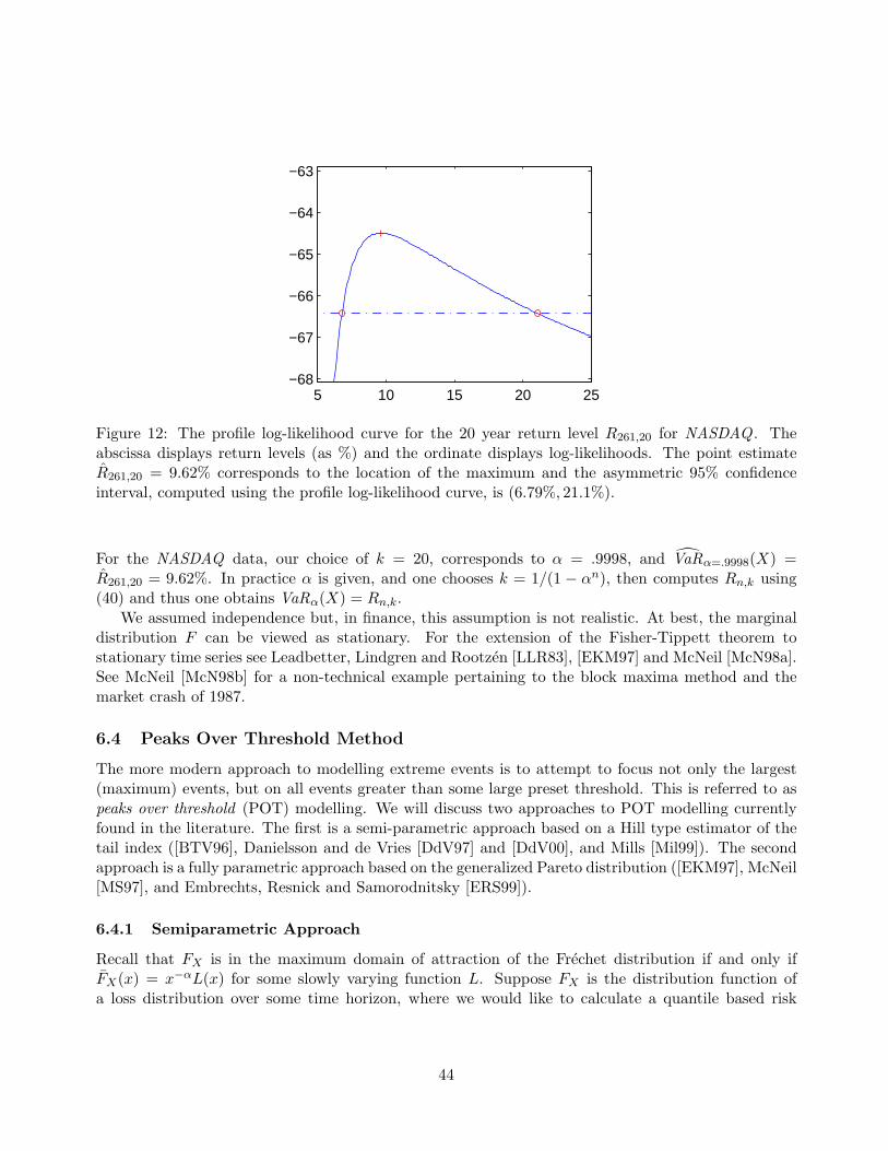
5 10 15 20 25−68

−67

−66

−65

−64

−63

Figure 12: The profile log-likelihood curve for the 20 year return level R261,20 for NASDAQ . Theabscissa displays return levels (as %) and the ordinate displays log-likelihoods. The point estimateR261,20 = 9.62% corresponds to the location of the maximum and the asymmetric 95% confidenceinterval, computed using the profile log-likelihood curve, is (6.79%, 21.1%).

For the NASDAQ data, our choice of k = 20, corresponds to α = .9998, and VaRα=.9998(X) =R261,20 = 9.62%. In practice α is given, and one chooses k = 1/(1 − αn), then computes Rn,k using(40) and thus one obtains VaRα(X) = Rn,k.

We assumed independence but, in finance, this assumption is not realistic. At best, the marginaldistribution F can be viewed as stationary. For the extension of the Fisher-Tippett theorem tostationary time series see Leadbetter, Lindgren and Rootzen [LLR83], [EKM97] and McNeil [McN98a].See McNeil [McN98b] for a non-technical example pertaining to the block maxima method and themarket crash of 1987.

6.4 Peaks Over Threshold Method

The more modern approach to modelling extreme events is to attempt to focus not only the largest(maximum) events, but on all events greater than some large preset threshold. This is referred to aspeaks over threshold (POT) modelling. We will discuss two approaches to POT modelling currentlyfound in the literature. The first is a semi-parametric approach based on a Hill type estimator of thetail index ([BTV96], Danielsson and de Vries [DdV97] and [DdV00], and Mills [Mil99]). The secondapproach is a fully parametric approach based on the generalized Pareto distribution ([EKM97], McNeil[MS97], and Embrechts, Resnick and Samorodnitsky [ERS99]).

6.4.1 Semiparametric Approach

Recall that FX is in the maximum domain of attraction of the Frechet distribution if and only ifFX(x) = x−αL(x) for some slowly varying function L. Suppose FX is the distribution function ofa loss distribution over some time horizon, where we would like to calculate a quantile based risk

44

measure such as VaR. Assume for simplicity that the distribution of large losses is of Pareto type

P(X > x) = cx−α , α > 0 , x > x0. (43)

The semi-parametric approach uses a Hill type estimator for α and order statistics of historical datato invert and solve for VaR.

We first focus on VaR. Let X(1) ≥ X(2) ≥ · · · ≥ X(n) be the order statistics of an historical sampleof losses of size n, assumed i.i.d. with distribution FX . If X is of Pareto type in the tail and X(k+1)

is a high order statistic then for x > X(k+1),

FX(x)FX(X(k+1))

=( x

X(k+1)

)−α.

The empirical distribution function estimator ˆFX(X(k+1)) = k/n suggests the following estimator ofFX in the upper tail,

FX(x) = 1− k

n

( x

X(k+1)

)−αforx > X(k+1).

By inverting this relation, one can express x in terms of FX(x), so that fixing q = FX(x) one gets48

x = VaRq(X). The value of q should be large, namely, q = FX(x) > F (X(k+1)) = 1−k/n. This yields

VaRq(X) = X(k+1)(n

k(1− q)

)−1/α. (44)

We obtained an estimator for VaR but it depends on k through X(k+1), on the sample size n andα. To estimate α, Hill [Hil75] proposed the following estimator α(Hill) which is also dependent on theorder statistics and sample size:

α(Hill) = α(Hill)k,n =

(1k

k∑i=1

lnX(i) − lnX(k+1)

)−1

. (45)

The consistency and asymptotic normality properties of this α(Hill) estimator are known in the i.i.d.case and for certain stationary processes. There are however, many issues surrounding Hill-typeestimators, see for example [BTV96], [EKM97] and Drees, de Haan and Resnick [DdHR00].

To obtain VaRq(X), one also needs to choose the threshold level X(k+1) or, equivalently, k. Daniels-son, de Haan, Peng and de Vries [DHPV01] provide an optimal choice for k by means of a two stagebootstrap method. Even in this case, however, optimal means merely minimizing the asymptoticmean squared error, which leaves the user uncertain as to how to proceed in the finite sample case.Traditionally the choice of k is done visually by constructing a Hill plot.

The Hill plot {(k, α(Hill)k,n ) : k = 1, . . . , n − 1} is a visual check for the optimal choice of k. The

choice of k and therefore of α(Hill)k,n , is inferred from a stable region of the plot since in the Pareto case,

where (43) holds, α(Hill)n−1,n is the maximum likelihood estimator for α. In the more general case

1− F (x) ∼ x−αL(x) , x →∞ , α > 0, (46)48We write here VaRq and not VaRα since now α represents the heavy-tail exponent.

45

0 100 200 300 4002

4

6

8

10Hill plot

k

Hk,

n

0 0.2 0.4 0.6 0.8 12

4

6

8

10

12

14AltHill plot

θ

Hnθ ,n

Figure 13: Hill plots for the NASDAQ data set. (Left) The Hill plot {(k, α(Hill)k,n ) : k = 1, . . . , n− 1}.

(Right) The AltHill plot{(θ, α(Hill)

dnθe,n) : 0 ≤ θ < 1}. The Hill plot is difficult to read, whereas the

AltHill plot gives the user an estimate of αAltHill ≈ 3.

where L is a slowly varying function, the traditional Hill plot is often difficult to interpret. Resnick andStarica [RS97] suggest an alternative plot, called an AltHill plot by plotting {(θ, α(Hill)

dnθe,n) : 0 ≤ θ < 1}where dnθe denotes the smallest integer greater than or equal to nθ. This plot has the advantage ofstretching the left hand side of the plot, which corresponds to smaller values of k, often making thechoice of k easier. See Figure 13 for examples of the Hill and AltHill plots for the ordered negativereturns X(j) for the NASDAQ .

6.4.2 Fully Parametric Approach

The fully parametric approach uses the generalized Pareto distribution (GPD) and the second funda-mental theorem in EVT by Pickands, Balkema and de Haan. The GPD is a two-parameter distribution

Gξ,β(x) =

1−(1 + ξx

β

)−1/ξ: ξ 6= 0

1− exp(−x

β

): ξ = 0,

where an additional parameter β > 0 has been introduced. The support of Gξ,β(x) is x ≥ 0 for ξ ≥ 0and 0 ≤ x ≤ −β/ξ for ξ < 0. The distribution is heavy-tailed when ξ > 0. GPD distributions withβ = 1 are displayed in Figure 14.

Definition 6.1 Let X ∼ F with right-end-point xF = sup{x ∈ R |F (x) < 1} ≤ ∞. For any highthreshold u < xF define the excess distribution function

Fu(x) = P(X − u ≤ x |X > u) for 0 ≤ x < xF − u. (47)

46

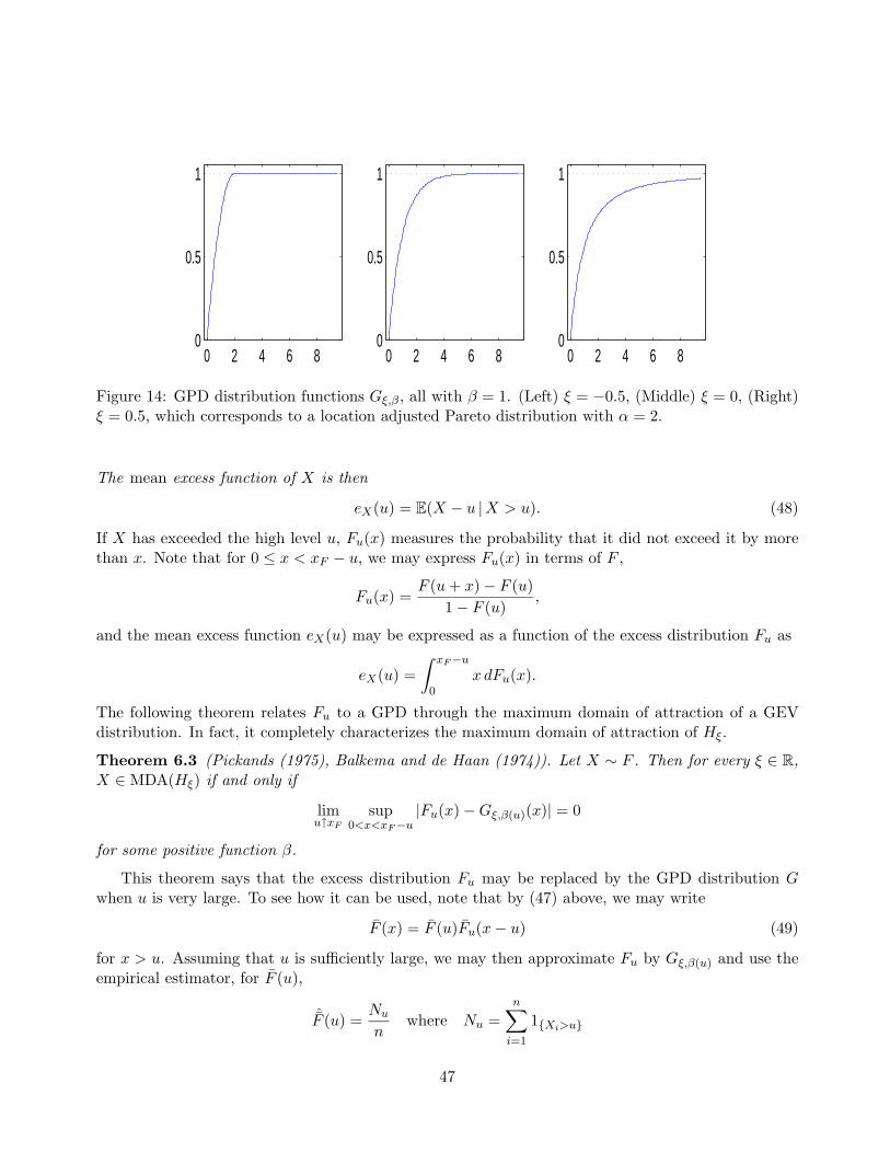
0 2 4 6 80

0.5

1

0 2 4 6 80

0.5

1

0 2 4 6 80

0.5

1

Figure 14: GPD distribution functions Gξ,β, all with β = 1. (Left) ξ = −0.5, (Middle) ξ = 0, (Right)ξ = 0.5, which corresponds to a location adjusted Pareto distribution with α = 2.

The mean excess function of X is then

eX(u) = E(X − u |X > u). (48)

If X has exceeded the high level u, Fu(x) measures the probability that it did not exceed it by morethan x. Note that for 0 ≤ x < xF − u, we may express Fu(x) in terms of F ,

Fu(x) =F (u + x)− F (u)

1− F (u),

and the mean excess function eX(u) may be expressed as a function of the excess distribution Fu as

eX(u) =∫ xF−u

0x dFu(x).

The following theorem relates Fu to a GPD through the maximum domain of attraction of a GEVdistribution. In fact, it completely characterizes the maximum domain of attraction of Hξ.

Theorem 6.3 (Pickands (1975), Balkema and de Haan (1974)). Let X ∼ F . Then for every ξ ∈ R,X ∈ MDA(Hξ) if and only if

limu↑xF

sup0<x<xF−u

|Fu(x)−Gξ,β(u)(x)| = 0

for some positive function β.

This theorem says that the excess distribution Fu may be replaced by the GPD distribution Gwhen u is very large. To see how it can be used, note that by (47) above, we may write

F (x) = F (u)Fu(x− u) (49)

for x > u. Assuming that u is sufficiently large, we may then approximate Fu by Gξ,β(u) and use theempirical estimator, for F (u),

ˆF (u) =Nu

nwhere Nu =

n∑i=1

1{Xi>u}

47

0 5 100

1

2

Figure 15: Sample mean excess plot (u, eX(u)) for NASDAQ .

and where n is the total number of observations. The upper tail of F (x) may then be estimated by

F (x) = 1− ˆF = 1− Nu

n

(1 + ξ

x− u

β

)−1/ξ

for all x > u. (50)

This way of doing things allows us to extrapolate beyond the available data which would not bepossible had we chosen an empirical estimator for F (x), x > u. We can therefore deal with potentiallycatastrophic events which have not yet occurred.

The parameters ξ and β of the GPD Gξ,β(u) may be estimated by using, for example, maximumlikelihood once the threshold u has been chosen. The data points that are used in the maximumlikelihood estimation are Xi1 − u, . . . , Xik − u where Xi1 , . . . , Xik are the observations that exceed u.Again there is a bias-variance trade-off in the choice of u. To choose a value for u, a graphical toolknown as the mean excess plot (u, eX(u)) is often used.

The mean excess plot relies on the following theorem for generalized Pareto distributions.

Theorem 6.4 ([EKM97]) Suppose X has GPD distribution with ξ < 1 and β. Then, for u < xF ,

eX(u) =β + ξu

1− ξ, β + ξu > 0.

The restriction ξ < 1 implies that the heavy-tailed distribution must have at least a finite mean.If the threshold u is large enough so that Fu is approximately Gξ,β then, by Theorem 6.4, the

plot (u, e(u)) is linear in u. How then is one to pick u? The mean excess plot is a graphical tool forexamining the relationship between the possible threshold u and the mean excess function eX(u) andchecking the values of u where there is linearity. In practice it is not eX(u), but its sample version

eX(u) =∑n

i=1(Xi − u)+∑ni=1 1{Xi>u}

which is plotted against u. After using the mean excess plot to pick the upper threshold u one obtainsan estimator of the tail of the distribution by applying (50). For the NASDAQ data, since linearityseems to start at relatively small values of u (Figure 15), we choose u = 1.59 which corresponds to the95% of the empirical NASDAQ return distribution.

48

1971 1974 1976 1979 1982 1984 1987 1990 1993 1995 1998

2000

4000

6000

1971 1974 1976 1979 1982 1984 1987 1990 1993 1995 1998

−10

0

10

1971 1974 1976 1979 1982 1984 1987 1990 1993 1995 1998

−10

0

10

Figure 16: Time series of NASDAQ daily prices, (log) returns and annual maxima and minima dailyreturns given as a percent for the period February 1971 (when it was created) to February 2001. IfPt is the price (level) at time t, the returns are defined as 100 ln(Pt/Pt−1) and expressed as %. Thecrash of 1987 is clearly visible. The NASDAQ price level peaked in March of 2000.

To obtain VaRα(X) for VaRα(X) > u, one simply inverts the tail estimator (50), which yields

VaRα(X) = u +β

ξ

((n

Nu(1− α)

)−ξ

− 1

). (51)

Since expected shortfall is a risk measure with better technical properties than VaR we would like tofind an estimator for it which uses our GPD model of the tail. Recalling the definitions of the expectedshortfall (22) and the mean excess function (48) we have that

Sα(X) = VaRα(X) + eX(VaRα(X)).

Since the excess distribution Fu is approximated by a GPD Gξ,β(u) with ξ < 1 then, applying Theo-rem 6.4, we get for VaRα(X) > u,

Sα(X) = VaRα(X) +β + ξ (VaRα(X)− u)

1− ξ=

β + VaRα(X)− ξu

1− ξ.

49

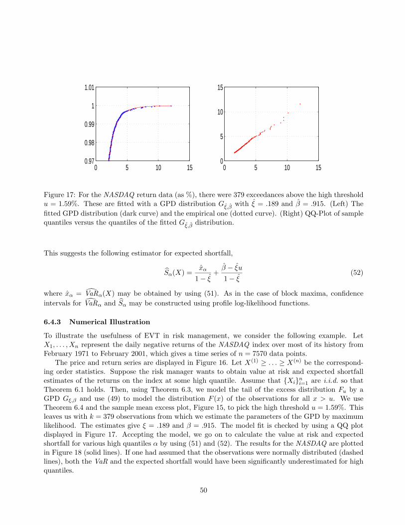
0 5 10 150

5

10

15

0 5 10 150.97

0.98

0.99

1

1.01

Figure 17: For the NASDAQ return data (as %), there were 379 exceedances above the high thresholdu = 1.59%. These are fitted with a GPD distribution Gξ,β with ξ = .189 and β = .915. (Left) Thefitted GPD distribution (dark curve) and the empirical one (dotted curve). (Right) QQ-Plot of samplequantiles versus the quantiles of the fitted Gξ,β distribution.

This suggests the following estimator for expected shortfall,

Sα(X) =xα

1− ξ+

β − ξu

1− ξ(52)

where xα = VaRα(X) may be obtained by using (51). As in the case of block maxima, confidenceintervals for VaRα and Sα may be constructed using profile log-likelihood functions.

6.4.3 Numerical Illustration

To illustrate the usefulness of EVT in risk management, we consider the following example. LetX1, . . . , Xn represent the daily negative returns of the NASDAQ index over most of its history fromFebruary 1971 to February 2001, which gives a time series of n = 7570 data points.

The price and return series are displayed in Figure 16. Let X(1) ≥ . . . ≥ X(n) be the correspond-ing order statistics. Suppose the risk manager wants to obtain value at risk and expected shortfallestimates of the returns on the index at some high quantile. Assume that {Xi}n

i=1 are i.i.d. so thatTheorem 6.1 holds. Then, using Theorem 6.3, we model the tail of the excess distribution Fu by aGPD Gξ,β and use (49) to model the distribution F (x) of the observations for all x > u. We useTheorem 6.4 and the sample mean excess plot, Figure 15, to pick the high threshold u = 1.59%. Thisleaves us with k = 379 observations from which we estimate the parameters of the GPD by maximumlikelihood. The estimates give ξ = .189 and β = .915. The model fit is checked by using a QQ plotdisplayed in Figure 17. Accepting the model, we go on to calculate the value at risk and expectedshortfall for various high quantiles α by using (51) and (52). The results for the NASDAQ are plottedin Figure 18 (solid lines). If one had assumed that the observations were normally distributed (dashedlines), both the VaR and the expected shortfall would have been significantly underestimated for highquantiles.

50

0.95 0.96 0.97 0.98 0.99 1

6

8

10

12

14

0.95 0.96 0.97 0.98 0.99 1

6

8

10

12

14

Figure 18: Risk estimates for NASDAQ in percent returns versus α. (Left) Value at risk VaRα,for GPD (solid) and normal (dashed). (Right) Expected shortfall Sα, for GDP (solid) and normal(dashed). The parameters of the GPD are fitted by maximum likelihood using 30 years of data. Thesample mean and volatility of the normal distribution are computed by (16) using the most recentyear of daily observations.

For example, at the α = .99 confidence level, VaRα(X) = 6.59% under the normal model versusVaRα(X) = 8.19% for the GPD model. For the expected shortfall, the difference is even moredramatic. For the normal model, Sα(X) = 7.09% versus Sα(X) = 10.8% for the GPD model. This isto be expected, since under the assumption of normality it may be shown ([EKM97]) that

Sα

VaRα−→ 1 as α → 1−,

whereas for the GPD modelSα

VaRα−→ 1

1− ξas α → 1−.

These results indicate that for very high quantiles, the expected shortfall Sα and the value at riskVaRα are comparable under normality, but for the GPD with ξ < 1, Sα tends to be larger than VaRα.

6.4.4 A GARCH-EVT model for Risk

In order to invoke Theorems 6.1 and 6.3 in the numerical illustration above it was necessary to assumethat the (negative) returns {Xt}t∈Z were i.i.d. However, from inspection of Figures 16 and 19, it isapparent that this assumption is unrealistic. The time series of returns is characterized by periods ofvarying volatility, that is, the time series is heteroscedastic. The heteroscadicity of the time series maycause problems for the estimation of the parameters of the GPD model since we would expect thehigh threshold u to be violated more often during periods of high volatility. Smith [Smi00] suggestsusing Bayesian techniques to model time-varying GPD parameters. In this section, we review a modelproposed by McNeil and Frey [MF00] which extends the EVT methodology to models of financial timeseries that allow for stochastic volatility and apply this model to the NASDAQ data set.

51

0 10 20 30−0.5

0

0.5

1

0 10 20 30−0.5

0

0.5

1

0 10 20 30−0.5

0

0.5

1

0 10 20 30−0.5

0

0.5

1

Figure 19: Sample auto correlation functions with lags on the abscissa and sample autocorrelation onthe ordinate: Returns (top left), squared Returns (bottom left), GARCH Innovations (top right),squared GARCH Innovations (bottom right). The sample consists of 1000 daily returns for theNASDAQ ending Feb. 2001. Horizontal lines indicate the 95% confidence bands (±1.96/

√n) cor-

responding to Gaussian white noise.

Recall from Section 3.2.2 that the standard GARCH(1,1) model is given by49

Xt = σtZt where Zt ∼ FZ i.i.d., (53)σ2

t = α0 + α1X2t−1 + β1σ

2t−1. (54)

Since the time t + 1 volatility σt+1 is known at time t we have that

V aRα(Xt+1 |Ft) := inf {x ∈ R |FXt+1 |Ft(x) ≥ α}

= σt+1zα, (55)

where zα = F−1Z (α). The same argument shows that the conditional expected shortfall

Sα(Xt+1 |Ft) := E (Xt+1 |Xt+1 > V aRα(Xt+1 |Ft) , Ft) = σt+1E(Z |Z > zα).49Since the NASDAQ series appears to have a zero conditional mean we do not set Xt = µt + σtZt and model the

mean µt, for example as an AR(1) process µt = φXt−1.

52

Traditionally the innovation distribution FZ is assumed normal. Figures 6 and 20 show that thisassumption may still underestimate the tails of the loss portion of the distribution. McNeil and Freypropose a two step procedure to estimate VaR and expected shortfall of the conditional distribution.First they use a GARCH(1,1) model for the volatility of the (negative) return series {Xt}. This givesa series of model implied innovations Zt = Xt/σt. Second, EVT is used to model the tails of thedistribution of these innovations. This approach has the obvious benefit that the resulting innovationsZt are much closer to satisfying the requirements of Theorems 6.1 and 6.3 than is the original series.We illustrate the methodology with an example using the NASDAQ data.

1. Let (xt−n+1, . . . , xt−1, xt) be n daily negative returns of the NASDAQ . We take50 n = 1000 anduse pseudo-maximum-likelihood (PML) to estimate the model parameters θ = (α0, α1, β1) in(54) under the assumption51 that FZ is normal in (53). The parameter vector θ depends on thetrue distribution of (Xt−n+1, . . . , Xt−1, Xt), which is assumed stationary, and on the distributionFZ used to compute the likelihood function52. When we assume FZ is normal we fit a modelwhose distributional assumptions we do not believe. Under standard regularity conditions thisis justified since θ is a consistent estimator of θ (in fact, asymptotically normal) even if FZ isnon normal. See Gourieroux [Gou97] and references therein for details.

2. The model innovations (zt−n+1, . . . , zt−1, zt) = (xt−n+1/σt−n+1, . . . , xt−1/σt−1, xt/σt) are nowcalculated. If the model is tenable, these innovations should be i.i.d. Figure 19 shows that whilethe i.i.d. assumption is not realistic for the series of returns, it is defensible for the series ofinnovations53. While the returns appear uncorrelated, their squares clearly are not, and hencethe returns are dependent. The GARCH innovations and their squares appear uncorrelated.The i.i.d. assumption is therefore more tenable.

3. Examination of the QQ plot of the innovations in Figure 20 reveals that the loss tail is heavierthan that of the normal. Therefore the EVT tools of Section 6.4.2 are now applied to theinnovations (zt−n+1, . . . , zt−1, zt). Let z(1) ≤ · · · ≤ z(n) be the order statistics of the innovationsample. We choose the threshold u = 1.79, again corresponding to the 95% of the empiricaldistribution of innovations, which leaves k = 50 observations (z(n−k+1), . . . , z(n)), from whichto estimate the GPD parameters by maximum likelihood. The estimates give ξ = .323 andβ = .364.

Observe that ξ = .323 corresponds to a heavier tail than ξ = .189 which we found in Section 6.4.3.We are fitting here, however, over a particularly volatile period of 1000 days of the NASDAQ endingFeb. 2001, whereas in Section 6.4.3, we considered nearly 30 years worth of returns where for themajority of the time the NASDAQ was significantly less volatile (see Figure 16).

Since the model is assumed stationary, we could, in principle, use the estimated GARCH parametersto compute σt+1 |Ft using (54) for t beyond Feb. 2001. Using zα corresponding to the GPD distributionGξ,β, we would obtain, by using (55), V aRα(Xt+1 |Ft) for t beyond Feb. 2001. In practice, however,

50We keep the sample size moderate in order to avoid the IGARCH effect, that is α1 + β1 = 1, corresponding tonon-stationarity. See [MS00] for details.

51The term pseudo refers to the fact that one is not maximizing the true likelihood.52The condition α1 + β1 < 1 is sufficient for stationarity of the GARCH model. We found α0 = .080, α1 = .181 and

β1 = .811. However, as indicated in the sequel, the GARCH model is constantly updated, and hence is never used on aninfinite horizon.

53Ljung-Box tests also found no evidence against the i.i.d. assumption for the innovations.

53

−10 −5 0 5 10−20

−10

0

10

20

−4 −2 0 2 4−5

0

5

Figure 20: QQ plots versus the normal for returns (left) and innovations (right) in Figure 19. Noticethat the lower (loss) tail of the innovations are still heavier than the normal distribution.

stationarity is not always assured and in any case one wants to use the most recent data available inorder to calibrate the model.

In order to backtest the methodology we use the most recent 500 days in our NASDAQ dataset. For each day, t + 1, in this data set we use the previous n = 1000 days (negative) returns(Xt−n+1, . . . , Xt−1, Xt) to calibrate the model and estimate V aRα(Xt+1 |Ft) for α = .95 and α = .99using the steps above. We compare V aRα(Xt+1 |Ft) with the actual loss xt+1. A violation, at the α

level, is said to occur whenever xt+1 > V aRα(Xt+1 |Ft). Results for the period ending Feb. 2001 aregiven in Figure 21.

7 Stable Paretian Models

The works of Mandelbrot [Man63] and Fama [Fam65] introduced the use of stable distributions tofinance. The excessively peaked and heavy-tailed nature of the return distribution led the authorsto reject the standard hypothesis of normally distributed returns in favor of the stable distribution.Since this time, the stable distribution has been used to model both the unconditional, and condi-tional return distributions. In addition, portfolio theories and market equilibrium models have beenconstructed using it. For an in depth introduction to the general properties of stable distributionssee Samorodnitsky and Taqqu [ST94] and the upcoming text Nolan [Nol01]. A major reference forapplications in finance is Rachev and Mittnik [RM00].

In Definition 3.2, the stable distribution Sα(σ, β, µ) is defined as the limiting distribution of thesum of i.i.d. random variables. Like the normal distribution, stable distributions are closed underaddition, and are often defined by this property. Recall that if X1 ∼ N(µ1, σ

21) and X2 ∼ N(µ2, σ

22)

are independent then X1 + X2 ∼ N(µ1 + µ2, σ21 + σ2

2). Similarly, for stable random variables, ifX1 ∼ Sα(σ1, β1, µ1) and X2 ∼ Sα(σ2, β2, µ2) are independent, then X1 + X2 ∼ Sα(σ, β, µ) where

σ = (σα1 + σα

2 )1/α , β =β1σ

α1 + β2σ

α2

σα1 + σα

2

, µ = µ1 + µ2.

54

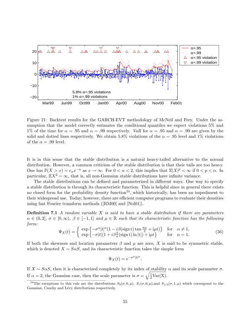
Mar99 Jun99 Oct99 Jan00 Apr00 Aug00 Nov00 Feb01

−20

−10

0

10

20

5.8% α=.95 violations1% α=.99 violations

α=.95α=.99α=.95 violationα=.99 violation

Figure 21: Backtest results for the GARCH-EVT methodology of McNeil and Frey. Under the as-sumption that the model correctly estimates the conditional quantiles we expect violations 5% and1% of the time for α = .95 and α = .99 respectively. VaR for α = .95 and α = .99 are given by thesolid and dotted lines respectively. We obtain 5.8% violations of the α = .95 level and 1% violationsof the α = .99 level.

It is in this sense that the stable distribution is a natural heavy-tailed alternative to the normaldistribution. However, a common criticism of the stable distribution is that their tails are too heavy.One has P(X > x) ∼ cαx−α as x →∞. For 0 < α < 2, this implies that E|X|p < ∞ if 0 < p < α. Inparticular, EX2 = ∞, that is, all non-Gaussian stable distributions have infinite variance.

The stable distributions can be defined and parameterized in different ways. One way to specifya stable distribution is through its characteristic function. This is helpful since in general there existsno closed form for the probability density function54, which historically, has been an impediment totheir widespread use. Today, however, there are efficient computer programs to evaluate their densitiesusing fast Fourier transform methods ([RM00] and [Nol01]).

Definition 7.1 A random variable X is said to have a stable distribution if there are parametersα ∈ (0, 2], σ ∈ [0,∞), β ∈ [−1, 1] and µ ∈ R such that its characteristic function has the followingform:

ΨX(t) ={

exp{−σα|t|α(1− iβ(sign t) tan πα

2 + iµt)}

for α 6= 1,exp

{−σ|t|(1 + iβ 2π (sign t) ln |t|) + iµt

}for α = 1.

(56)

If both the skewness and location parameters β and µ are zero, X is said to be symmetric stable,which is denoted X ∼ SαS, and its characteristic function takes the simple form

ΨX(t) = e−σα|t|α .

If X ∼ SαS, then it is characterized completely by its index of stability α and its scale parameter σ.

If α = 2, the Gaussian case, then the scale parameter is σ =√

12Var(X).

54The exceptions to this rule are the distributions S2(σ, 0, µ), S1(σ, 0, µ),and S1/2(σ, 1, µ) which correspond to theGaussian, Cauchy and Levy distributions respectively.

55

7.1 Stable Portfolio Theory

In Section 2.2 we introduced the mean-variance portfolio theory of Markowitz. The model assumedthat the distribution of asset returns is multivariate normal, and provides efficient portfolios, thatis, portfolios with maximum expected return for a given level of risk, where risk is measured by thevariance of the portfolio. It is possible to extend the ideas of portfolio theory to the case where assetreturns have a multivariate stable distribution, even though, variances are now infinite. We need firstto define a stable random vector and specify its characteristic function.

Definition 7.2 The random vector X = (X1, . . . , Xn) is said to be a stable random vector in Rn iffor any a, b > 0 there exists c > 0 and d ∈ Rn such that

aX1 + bX2d= cX + d (57)

where Xj, j = 1, 2 are independent copies of X.

The constants in (57) are related by cα = aα + bα, where α ∈ (0, 2] is the index of stability. Settingn = 1 in (57) yields one of the alternate definitions of a stable random variable alluded to earlier. Inthe case of a stable random vector, the scale and skewness parameters σ and β are replaced by a finitemeasure ΓX on the unit hypersphere in Rn. For convenience here, let (·, ·) denote the inner productso that (t, s) =

∑ni=1 tisi

55.

Theorem 7.1 Let 0 < α < 2. Then X = (X1, . . . , Xn) is a stable random vector with index of stabilityα if and only if there exists a finite measure ΓX on the unit hypersphere Sn = {s ∈ Rn | ‖s‖ = 1} anda vector µ ∈ Rn such that

Ψα(t) =

exp{− ∫

Sn|(t, s)|α (

1− isign((t, s)) tan πα2

)ΓX(ds) + i(t, µ)

}for α 6= 1,

exp{− ∫

Sn|(t, s)| (1 + i 2

π sign((t, s)) ln |(t, s)|) ΓX(ds) + i(t, µ)}

for α = 1.(58)

The pair (ΓX, µ) is unique.

The measure ΓX is called the spectral measure of the stable random vector X and specifies thedependence structure. If X is SαS in Rn, then the characteristic function takes the simple form

Ψα(t) = exp{−

∫Sn

|(t, s)|αΓX(ds)}

,

where Γ is the unique symmetric spectral measure. The expression in (58) for the characteristic func-tion is also valid for the normal case α = 2. When α = 2, it reduces to Ψ2(t) = exp

{− ∫

Sn|(t, s)|2ΓX(ds)

}but in this case ΓX is no longer unique. To get a feeling for ΓX, suppose X = (X1, X2) and that thedistribution is Gaussian. Then∫

S2

|(t, s)|2Γ(X1,X2)(ds) =∫

S2

|(t1s1 + t2s2)|2Γ(X1,X2)(ds)

= t21σ21 + 2t1t2σ1,2 + t21σ

21

55Previously we wrote tT s instead of (t, s).

56

whereσ2

i =∫

S2

s2i Γ(X1,X2)(ds), i = 1, 2 and σ1,2 =

∫S2

s1s2Γ(X1,X2)(ds),

and where integration over the circle S2 means integration on {s = (s1, s2) | s21+s2

2 = 1}. One recognizesthe normal characteristic function with VarX1 = 2σ2

1, VarX2 = 2σ22 and Cov(X1, X2) = 2σ1,2. Since

different choices of Γ(X1,X2) can yield the same values for σ21, σ2

2 and σ1,2, the choice of ΓX is notunique in the Gaussian case.

As in the case of a normal random vector, if X is multivariate stable with index of stability0 < α < 2, then all linear combinations of the components of X are stable with the same α. So,if X is a stable random vector in Rn, and w ∈ Rn, we know that Y = (w, X) =

∑ni=1 wiXi is

Sα(σY , βY , µY ). Using the characteristic function (58), it can be shown (see [ST94], Example 2.3.4),that

σY =(∫

Sn

|(w, s)|αΓX(ds))1/α

, (59)

βY =

∫Sn|(w, s)|αsign(w, s)ΓX(ds)∫

Sn|(w, s)|αΓX(ds)

, (60)

µY ={

(w, µ) for α 6= 1,(w, µ)− 2

π

∫Sn

(w, s) ln |(w, s)|ΓX(ds) for α = 1.(61)

In the mean-variance portfolio theory, the risk to be minimized for any level of expected return isgiven by the portfolios’ variance. If the asset returns are assumed multivariate stable with index ofstability 0 < α < 2 then the variance is infinite and cannot be used. In the stable portfolio theory,it is assumed that 1 < α < 2, EX = µ and that X − µ ∼ SαS. Let w be the vector of weights forthe risky portfolio Xp = (w,X). Given the relationship between the scale parameter and the variancein the Gaussian case (that is, stable with α = 2), it is natural to use the scale parameter σXp of theresulting stable distribution instead of the standard deviation. It is given by (59). This brings us tothe corresponding stable portfolio problem:

minw

σXp =(∫

Sn

|(w, s)|αΓX(ds))1/α

,

such that (w, µ) ≥ a, (62)(w, e) = 1.

The risk measure σXp = σ(w,X) is a convex function of w and the problem is generally solved usingsequential quadratic programming. See Belkacem [Bel97] and [RM00] and references therein for detailsof the procedure and on the estimation of the index of stability, spectral measure and scale parameters.If a risk free asset is included in the asset universe, then we end up with a maximization problem similarto (2) in Section 2.2, but where the risk measure is the scale parameter σXp of the risky portfolio.

7.2 Stable Asset Pricing

Since there exists a portfolio theory under the assumption of a multivariate stable distribution of assetreturns (1 < α < 2), it is natural to ask whether there exists an analogous CAPM. The answer is

57

positive, and it was first introduced by Fama [Fam70]. For recent descriptions of the stable CAPMsee Belkacem, Levy Vehel and Walter [BVW96] and, of course, Rachev and Mittnik [RM00].

The assumptions behind the stable CAPM are the same as in the Gaussian case in Section 2.3 withthe assumption of joint normality of asset returns replaced by that of jointly stable asset returns withindex of stability α ∈ (1, 2). That is, we assume EX = µ and that X − µ ∼ SαS. Recall from thetraditional CAPM and Equations (3) and (4), that the expected premium of holding the risky asseti over the riskless asset is proportional to the expected premium of holding the market portfolio overthe riskless asset. The constant of proportionality was the risky assets beta given by (4). In the stableCAPM, we require an alternative measure of dependence since covariances do not exist. Naturally,the scale parameter σ replaces the standard deviation.

The covariation is a natural alternative to the covariance in the stable case when 1 < α < 2. Thismeasure possesses many, but not all, of the useful properties of covariance in the Gaussian case. Wedefine and present several of the properties of covariation. Details may be found in [ST94] and [RM00].

Definition 7.3 Let X1 and X2 be jointly SαS with 1 < α ≤ 2 and let Γ(X1,X2) be the spectral measureof the random vector (X1, X2). The covariation of X1 on X2 is given by

[X1, X2]α =∫

S2

s1s<α−1>2 Γ(X1,X2)(ds) (63)

where s<p> denotes the signed power s<p> = |s|p(sign s).

In the Gaussian case α = 2 it reduces to

[X1, X2]2 =12Cov(X1, X2). (64)

Note, however, that whereas in the Gaussian case the dependence structure is fully characterized bythe covariance, in the stable one needs to use ΓX, and the covariation does not fully characterize thedependence structure. We now derive the stable CAPM under the preceding assumptions, following[BVW96].

Consider a portfolio of a riskless asset with rate of return r and a risky asset Xi with weights wand 1 − w respectively. The expected rate of return of the portfolio Xp = wr + (1 − w)Xi is thenEXp = wr + (1 − w)EXi, and its risk, as given by its scale parameter, is σp = (1 − w)σi

56. Therisk-return trade-off is then given by

EXp = r +EXi − r

σiσp (65)

after setting w = 1 − σp/σi. Under the assumptions of CAPM, investors have homogeneous beliefs,that is, they all agree on the multivariate stable parameters. This means that all investors hold themarket portfolio (as in Section 2.3) as their risky asset and the risk-return trade-off (65) becomes

EXp = r +EXM − r

σMσp. (66)

where XM and σM are the rate of return and scale parameter respectively of the market.

56Note that if X ∼ Sα(σ, β, µ) then aX + b ∼ Sα(|a|σ, sign(a)β, aµ + b) if 1 < α < 2.

58

M

σ

µ

rP

Figure 22: The stable efficient frontier. The portfolio Xp = wXi + (1 − w)XM is suboptimal, andhence must be dominated by the efficient frontier.

Now consider the suboptimal portfolio Xp = wXi + (1−w)XM obtained by adding to the marketportfolio a certain position in asset i (the portfolio is optimal if w = 0). Since X −µ ∼ SαS we knowthat Xi − µi and XM − µM are jointly SαS. By properties of symmetric stable random vectors thismeans that Xp ∼ Sα(σp, 0, µp), where the scale and location parameters are given by (59) and (61),that is

σαp =

∫S2

|ws1 + (1− w)s2|αΓ(Xi,Xp)(ds1, ds2), (67)

µp = EXp = wµi + (1− w)µM , (68)

respectively. Differentiating with respect to w gives

∂µp

∂w= µi − µM , (69)

∂σp

∂w=

1ασα−1

p

∂σαp

∂w=

1σα−1

p

∫S2

(s1 − s2)(ws1 + (1− w)s2)<α−1>Γ(Xi,Xp)(ds1, ds2). (70)

So evaluating (69) and (70) at w = 0 and using Definition 7.3 we get

∂µp

∂σp

∣∣∣∣w=0

=∂µp

∂w

/∂σp

∂w

∣∣∣∣w=0

=σα−1

M (µi − µM )[Xi, XM ]α − σα

M

, (71)

since at w = 0 the portfolio Xp becomes XM and σp becomes σM . Moreover, in market equilibriumthe trade-off between risk and return is given by (66), so that the slope ∂µp/∂σp at w = 0 is given by(µM − r)/σM (see Figure 22). Hence

µM − r

σM=

σα−1M (µi − µM )

[Xi, XM ]α − σαM

. (72)

59

This may be rewritten in the familiar CAPM form (3) as

E(Xi − r) = βiE(XM − r),

where now, in the stable case,

βi =[Xi, XM ]α

σαM

. (73)

Note that if we assume Gaussian returns, then X − µ ∼ SαS with α = 2, and by using (64), werecover

βi =Cov(Xi, XM )

Var(XM ),

that is, the traditional CAPM result.

Acknowledgments

We would like to thank Paul Embrechts and Filip Lindskog for many valuable comments which ledto an improved exposition of this material. This research was partially supported by the NSF GrantANI-9805623 at Boston University.

References

[ADEH97] P. Artzner, F. Delbaen, J.M. Eber, and D. Heath. Thinking coherently. RISK, 10(11), 1997.

[ADEH99] P. Artzner, F. Delbaen, J.M. Eber, and D. Heath. Coherent measures of risk. Mathematical Finance,9(3):203–228, 1999.

[Alb97] C. Albanese. Credit exposure. Diversification risk and coherent VaR. Preprint, Department ofMathematics, University of Toronto, 1997.

[BCK92] T. Bollerslev, R.Y. Chou, and K.F. Kroner. ARCH modelling in finance: A review of the theoryand empirical evidence. Journal of Econometrics, 52:307–327, 1992.

[Bel97] L. Belkacem. How to select optimal portfolio in α-stable markets. Preprint, INRIA, 1997.

[Ber96] P. L. Bernstein. Against the Gods: The Remarkable Story of Risk. John Wiley & Sons, Inc., 1996.

[BG98] M. Broadie and P. Glasserman. Simulation for option pricing and risk management. In C. Alexander,editor, Risk Management and Analysis. John Wiley & Sons, 1998.

[BLS00] D. Bertsimas, G. J. Lauprete, and A. Samarov. Shortfall as a risk measure: Properties, optimizationand application. Preprint, MIT, 2000.

[BN77] O.E. Barndorff-Neilsen. Exponentially decreasing distributions for the logarithm of particle size.Proceeding of the Royal Society London A, 1977.

[Bol86] T. Bollerslev. Generalized autoregressive conditional heteroscadicity. Journal of Econometrics,31(1):34–105, 1986.

[BS73] F. Black and M. Scholes. The pricing of options and corporate liabilities. Journal of PoliticalEconomy, 81:637–654, 1973.

[BTV96] J. Beirlant, J.L. Teugels, and P. Vynckier. Practical Analysis of Extreme Values. Leuven UniversityPress, 1996.

60

[BVW96] L. Belkacem, J. Levy Vehel, and C. Walter. CAPM, risk and portfolio selection in stable markets.Preprint, INRIA, 1996.

[CPB00] P. Cizeau, M. Potters, and J-P Bouchaud. Correlations of extreme stock returns within a non-Gaussian one-factor model. Preprint, Science & Finance, 2000.

[DdHR00] H. Drees, L. de Haan, and S. Resnick. How to make a Hill plot. The Annals of Statistics, 28(1):254–274, 2000.

[DdV97] J. Danielsson and C. de Vries. Beyond the sample: Extreme quantile and probability estimation.Preprint, LSE, 1997.

[DdV00] J. Danielsson and C. de Vries. Value at risk and extreme returns. In P. Embrechts, editor, Extremesand Integrated Risk Management, pages 85–106. Risk Books, 2000.

[DHPV01] J. Danielsson, L. De Haan, L. Peng, and C.G. De Vries. Using a bootstrap method to choose thesample fraction in the tail index estimation. Journal of Multivariate Analysis, 76:226–248, 2001.

[DHV98] J. Danielsson, P. Hartmann, and C.G. De Vries. The cost of conservatism: Extreme returns, valueat risk and the Basle multiplication factor. RISK, 11:101–103, 1998.

[Dow98] K. Dowd. Beyond Value at Risk: The New Science of Risk Management. John Wiley & Sons, Inc.,1998.

[DP97] D. Duffie and J. Pan. An overview of value at risk. Journal of Derivatives, 4(3):7–49, 1997.

[DSS00] F.X. Diebold, T. Schuermann, and J.D. Stroughair. Pitfalls and opportunities in the use of extremevalue theory in risk management. Journal of Risk Finance, 1(Winter):30–36, 2000.

[EK95] E. Eberlein and U. Keller. Hyperbolic distributions in finance. Bernoulli, 1:281–299, 1995.

[EKM97] P. Embrechts, C. Kluppelberg, and T. Mikosch. Modelling Extremal Events for Insurance andFinance. Springer Berlin, 1997.

[ELM01] P. Embrechts, F. Lindskog, and A. McNeil. Modelling dependence with copulas and applications torisk management. 2001. In this volume.

[Emb00] P. Embrechts. Extreme value theory: Potential and limitations as an integrated risk managementtool. Derivatives Use, Trdaing & Regulation, 6:449–456, 2000.

[EMS99] P. Embrechts, A.J. McNeil, and D. Straumann. Correlation: Pitfalls and alternatives. RISK,12(5):69–71, 1999.

[EMS01] P. Embrechts, A.J. McNeil, and D. Straumann. Correlation and dependence in risk management:Properties and pitfalls. In M. Dempster and H.K. Moffatt, editors, Risk Management: Value at Riskand Beyond. Cambridge University Press, 2001. To appear.

[Eng82] R.F. Engle. Autoregressive conditional heteroscadicity with estimates of the variance of U.K. infla-tion. Econometrica, 50:987–1008, 1982.

[EP00] E. Eberlein and K. Prause. The generalized hyperbolic model: Financial derivatives and risk mea-sures. Preprint, FDM, University of Freiburg, 2000.

[ERS99] P. Embrechts, S.I. Resnick, and G. Samorodnitsky. Extreme value theory as a risk managementtool. North American Actuarial Journal, 3:30–41, 1999.

[Fam65] E.F. Fama. The behavior of stock market prices. Journal of Business, 38(1):34–105, 1965.

[Fam70] E.F. Fama. Risk, return and equilibrium. Journal of Political Economy, 79(1):30–55, 1970.

[FKN90] K.T. Fang, S. Kotz, and K.W. Ng. Symmetric Multivariate and Related Distributions. Chapman &Hall, 1990.

61

[Fra79] M. Frank. On the simultaneous associativity of F (x, y) and x+ y−F (x, y). Aequationes Mathemat-icae, 19:194–226, 1979.

[FV98] E.W Frees and E.A. Valdez. Understanding relationships using copulas. North Americal ActuarialJournal, 2(1):1–25, 1998.

[Gou97] C. Gourieroux. ARCH Models and Financial Applications. Springer-Verlag, 1997.

[Hil75] B.M. Hill. A simple general approach to inference about the tail of a distribution. Annals ofStatistics, 3(5):1163–1174, 1975.

[HL88] C. Huang and R. Litzenberger. Foundations of Financial Economics. North-Holland, N.Y., 1988.

[HW87] J. Hull and A. White. The pricing of options on assets with stochastic volatilities. Journal ofFinance, 2:281–300, 1987.

[Ing87] J. E. Ingersoll. Theory of Financial Decision Making. Rowman & Littlefield, 1987.

[Joe97] H. Joe. Multivariate Models and Dependence Concepts. Chapman & Hall, 1997.

[Jor01] P. Jorion. Value at Risk: The New Benchmark for Controlling Market Risk. McGraw-Hill, 2 edition,2001.

[KG00] E. Kellezi and M. Gilli. Extreme value theory for tail-related risk measures. Preprint, University ofGeneva, 2000.

[Lin65] J. Lintner. The valuation of risky assets and the selection of risky investment in stock portfolios andcapital budgets. Review of Economics and Statistics, 47:13–37, 1965.

[Lin00a] F. Lindskog. Linear correlation estimation. Preprint, ETH Zurich, 2000.

[Lin00b] F. Lindskog. Modelling dependence with copulas. Master’s thesis, ETH Zurich, 2000.

[LK78] H. Levy and Y. Kroll. Ordering uncertain options with borrowing and lending. Journal of Finance,33:553–573, 1978.

[LLR83] M.R. Leadbetter, G. Lindgren, and H. Rootzen. Extremes and Related Properties of Random Se-quences and Processes. Springer Verlag, 1983.

[Man63] B.B. Mandelbrot. The variation of certain speculative prices. Journal of Business, 36:392–417, 1963.

[Mar52] H. Markowitz. Portfolio selection. Journal of Finance, 7:77–91, 1952.

[Mar59] H. Markowitz. Portfolio Selection: Efficient Diversification of Investments. John Wiley & Sons,Inc., 1959.

[McN98a] A. McNeil. Calculating quantile risk measures for financial return series using extreme value theory.Preprint, ETH Zurich, 1998.

[McN98b] A. McNeil. On extremes and crashes. RISK, January, 1998.

[Met96] Risk Metrics. Technical document. Technical report, J.P Morgan, 1996.

[MF00] A. McNeil and R. Frey. Estimation of tail-related risk measures for heteroscedastic financial timeseries: An extreme value approach. Journal of Empirical Finance, 7:271–300, 2000.

[Mil99] T.C. Mills. The Econometric Modelling of Financial Time Series. Cambridge University Press,1999.

[MPR97] S. Mittnik, M.S. Paolella, and T. Rachev. Modelling the persistence of conditional volatilities withGARCH-stable processes. Preprint, University of California, Santa Barbara, 1997.

62

[MRP98] S. Mittnik, T. Rachev, and M.S. Paolella. Stable Paretian modelling in finance: Some empirical andtheoretical aspects. In Adler et al, editor, A Practicul Guide to Heavy Tails. Birkhauser, 1998.

[MS97] A. McNeil and T. Saladin. The peaks over threshold method for estimating high quantiles of lossdistributions. In Proceedings of the 28th International ASTIN Colloquium, 1997.

[MS00] T Mikosch and C. Starica. Change of structure in financial time series, long range dependence andthe GARCH model. Preprint, 2000.

[Nel99] R.B. Nelsen. An Introduction to Copulas. Springer, New York, 1999.

[Nol01] J. Nolan. Stable Distribution: Models for Heavy-Tailed data. Birkhauser, 2001.

[oBS5a] Basle Committee on Banking Supervision. An internal model-based approach to market risk capitalrequirements. Technical report, Balse, Switzerland: Basle Committee on Banking Supervision,1995a.

[oBS5b] Basle Committee on Banking Supervision. Planned supplement to the capital accord to incorporatemarket risks. Technical report, Balse, Switzerland: Basle Committee on Banking Supervision, 1995b.

[PMR95] A.K Panorska, S. Mittnik, and T. Rachev. Stable GARCH models for financial time series. AppliedMathematics Letters, 8:33–37, 1995.

[RM00] S. Rachev and S. Mittnik. Stable Paretian Models in Finance. John Wiley & Sons, 2000.

[Ros76] S.A. Ross. The arbitrage theory of capital asset pricing. Journal of Economic Theory, 13:341–360,1976.

[RS97] S. Resnick and C. Starica. Smoothing the Hill estimator. Advances in Applied Probability, 29, 1997.

[RT01] R-D Reiss and M. Thomas. Statistical Analysis of Extreme Values. Birkhauser, 2 edition, 2001.

[Sha64] W.F. Sharpe. Capital asset prices: A theory of market equilibrium under conditions of risk. Journalof Finance, 19:425–442, 1964.

[Shi99] A.N. Shiryaev. Essentials of Stochastic Finance. World Scientific, 1999.

[Skl96] A. Sklar. Random variables, distribution functions, and copulas - a personal look backward andforward. In Ruschendorff et al, editor, Distributions with Fixed Marginals and Related Topics.Hayward, CA. Institute of Mathematical Sciences, 1996.

[Smi00] R. Smith. Measuring risk with extreme value theory. In P. Embrechts, editor, Extremes and Inte-grated Risk Management, pages 19–35. Risk Books, 2000.

[ST94] G. Samorodnitsky and M. Taqqu. Stable Non-Gaussian Random Processes. Chapman & Hall, 1994.

[Sta97] G. Stahl. Three cheers. RISK, 10:67–69, 1997.

[Wil98] T.C. Wilson. Value at risk. In C. Alexander, editor, Risk Management and Analysis. John Wiley &Sons, 1998.

Brendan O. Bradley and Murad S. TaqquDepartment of Mathematics and StatisticsBoston University111 Cummington StreetBoston, MA 02215email: bbradley@bu.eduemail: murad@bu.eduweb: http://math.bu.edu/people/murad

63