FINANCIAL MANAGEMENT AND ACCOUNTING FUNDAMENTALS …

P1: OSO

manual JWBT106-Halpin April 27, 2009 21:7 Printer: Yet to come

FINANCIAL MANAGEMENT ANDACCOUNTING FUNDAMENTALSFOR CONSTRUCTION

i

FINANCIAL MANAGEMENT AND A CCOUN TlNG FUNDAMENTALS FOR CONS TRUC TlON DANIEL W. HALPIN, BOLIVAR A. SENIOR

Copyright 0 2009 by John Wiley & Sons, Inc. All rights reserved

P1: OSO


FINANCIALMANAGEMENT ANDACCOUNTINGFUNDAMENTALS FORCONSTRUCTION

DANIEL W. HALPIN, PURDUE UNIVERSITYBOLIVAR A. SENIOR, COLORADO STATE UNIVERSITY

A JOHN WILEY & SONS, INC.

iii

P1: OSO


This book is printed on acid-free paper.∞©

Copyright C© 2009 by John Wiley & Sons, Inc. All rights reserved.

Published by John Wiley & Sons, Inc., Hoboken, New Jersey.Published simultaneously in Canada.

No part of this publication may be reproduced, stored in a retrieval system, or transmitted in any form orby any means, electronic, mechanical, photocopying, recording, scanning, or otherwise, except aspermitted under Section 107 or 108 of the 1976 United States Copyright Act, without either the priorwritten permission of the Publisher, or authorization through payment of the appropriate per-copy fee tothe Copyright Clearance Center, 222 Rosewood Drive, Danvers, MA 01923, (978) 750-8400, fax (978)646-8600, or on the web at www.copyright.com. Requests to thePublisher for permissionshould be addressed to the Permissions Department, John Wiley& Sons, Inc., 111 River Street,Hoboken, NJ 07030, (201) 748-6011, fax (201) 748-6008, or online at www.wiley.com/go/permissions.

Limit of Liability/Disclaimer of Warranty: While the publisher and the author have used their best effortsin preparing this book, they make no representations or warranties with respect to the accuracy orcompleteness of the contents of this book and specifically disclaim any implied warranties ofmerchantability or fitness for a particular purpose. No warranty may be created or extended by salesrepresentatives or written sales materials. The advice and strategies contained herein may not be suitablefor your situation. You should consult with a professional where appropriate. Neither the publisher northe author shall be liable for any loss of profit or any other commercial damages, including but notlimited to special, incidental, consequential, or other damages.

For general information about our other products and services, please contact our Customer CareDepartment within the United States at (800) 762-2974, outside the United States at (317) 572-3993 orfax (317) 572-4002.

Wiley also publishes its books in a variety of electronic formats. Some content that appears in print maynot be available in electronic books. For more information about Wiley products, visit our web site atwww.wiley.com.

Library of Congress Cataloging-in-Publication Data:

Halpin, Daniel W.Financial management and accounting fundamentals for construction /

Daniel W. Halpin and Bolivar A. Senior.p. cm.

Includes index.ISBN 978-0-470-18271-0 (cloth)

1. Building–Estimates. 2. Construction industry–Accounting. 3. Building–Cost control.4. Construction industry–Finance. I. Senior, Bolivar A. II. Title.

TH435.H323 2009690.068′1–dc22 2009009715

Printed in the United States of America

10 9 8 7 6 5 4 3 2 1

iv

P1: OSO


CONTENTS

PREFACE xi

1 INTRODUCTION 1

The Big Paradox / 1What is Financial Management? / 2

First Stop: Financial Accounting / 2Why Construction Accounting Is Different from Accounting in

Other Business Sectors / 4Who Is at Risk? / 5Projects: The Output of the Construction Process / 6

Project-Level Controls / 7Time Value of Money / 8Entrepreneurial Issues / 8Review Questions and Exercises / 9

2 UNDERSTANDING FINANCIAL STATEMENTS 11

Introduction / 11Why Should You Care about Accounting? / 12Generally Accepted Accounting Principles / 12Cash and Accrual Bases: Two Ways to Look at Accounting / 13Cash Basis of Accounting / 14Accrual Basis of Accounting / 15

v

P1: OSO


vi CONTENTS

Accounts / 16Account Hierarchy / 16Financial Reports / 17Balance Sheet Layout / 21Balance Sheet Account Categories in Detail / 21The Fundamental Accounting Equation / 22Asset Values / 23The Fundamental Equation and Owners” Risk / 24Balance Sheet for Fudd Associates, Inc. / 24Key Accounts / 26The Income Statement / 29

Revisiting the Airport Screen / 31Components of an Income Statement – More Details / 32

The Accounting Tower of Babel / 34The Statement of Cash Flows / 35Contract Backlog / 37Public Corporations / 38Review Questions and Exercises / 39

3 ANALYZING COMPANY FINANCIAL DATA 43

Introduction / 43Vertical and Horizontal Analyses / 44

Vertical Analysis: Financial Ratios / 44Liquidity Indicators: Can This Company Get Cash in a Hurry? / 45

Current Ratio / 45Quick Ratio / 46Working Capital / 47

Profitability Indicators: Is This Company Making Enough Profit / 48Return on Equity / 48Return on Revenue / 50Return on Assets / 51Earnings Per Share / 51

Efficiency Indicators: How Long Does It Take a Company to Turnover Its Money / 52

Average Age of Inventory / 53Average Age of Accounts Payable / 56Other Average Ages / 57Operating Cycle / 57

P1: OSO


CONTENTS vii

Turnover Ratios / 58Revenue to Assets Turnover / 58

Capital Structure Indicators: How Committed Are the Owners?/ 59Debt to Equity / 60Assets to Equity (Leverage) / 60

Other Indicators / 60Horizontal Analysis: Tracking Financial Trends / 62Time Series Graphs / 62

Index-Number Trend Series / 63Conclusion / 63Review Questions and Exercises / 64

4 ACCOUNTING BASICS 71

Introduction / 71Transaction Processing / 71Journalizing the Transaction / 73

A Transaction to Enter Initializing Capital / 74A Vendor Billing Transaction / 74A Billing to the Client / 76

Posting Entries to the Ledger / 78Relationship of Work-in-Progress and Revenue/Expense Accounts / 80Closing the Accounting Cycle / 82Recognition of Income / 83

Percentage-of-Completion Method of Income Recognition / 83Completed-Contract Method of Income Recognition / 85

Transactions during a Period / 86Posting to the General Ledger during the Accounting Period / 88Closing Actions at the End of the Period / 91Review Questions and Exercises / 93

5 PROJECT-LEVEL COST CONTROL 97

Objectives of Project-Level Cost Control in Construction / 97Unique Aspects of Construction Cost Control / 98Types of Costs / 99The Construction Estimate / 99Cost Control System / 101Building a Cost Control System / 101Cost Accounts / 103Cost Account Structure / 104

P1: OSO


viii CONTENTS

Project Cost Code Structure / 106Cost Accounts for Integrated Project Management / 110Earned Value Analysis / 113Labor Data Cost Collection / 122Review Questions and Exercises / 125

6 FORECASTING FINANCIAL NEEDS 129

Importance of Cash Management / 129Understanding Cash Flow / 129Retainage / 131Project Cost, Value, and Cash Profiles / 131Cash Flow Calculation - A Simple Example / 133Peak Financial Requirements / 136Getting Help from the Owner / 137Optimizing Cash Flow / 138Project Cash Flow Estimates / 141Using Software for Cash Flow Computations / 144Company-Level Cash Flow Planning / 145Strategic Cash Flow Management: “Cash Farming? / 145Project and General Overhead / 146Fixed Overhead / 148Considerations in Establishing Fixed Overhead / 149Breakeven Analysis / 151Basic Relationships Governing the Breakeven Point / 154Review Questions and Exercises / 156

7 TIME VALUE OF MONEY AND EVALUATING INVESTMENTS 161

Introduction / 161Time Value of Money / 162Interest / 162Simple and Compound Interest / 163Nominal and Effective Rate / 165Equivalence and MARR / 166Discount Rate / 167Importance of Equivalence / 167Inflation / 168Sunk Costs / 169Cash Flow Diagrams / 169Annuities / 171

P1: OSO


CONTENTS ix

Conditions for Annuity Calculations / 173Calculating the Future Value of a Series of Payments / 174Summary of Equivalence Formulas / 175Worth Analysis Techniques: An Overview / 176Present Worth Analysis / 179Investments with Different Life Spans / 180Equivalent Annual Worth (EAW) / 181Internal Rate of Return / 183Limitations of the IRR Method / 185An Example Involving Cost Recovery / 186Comparison Using EAW / 188An IRR Example–Owner Financing Using Bonds / 191Review Questions and Exercises / 194

8 CONSTRUCTION LOANS AND CREDIT 199

Introduction / 199The Construction Financing Process / 200A Sample Developmental Project / 202The Amount of the Loan / 204How Is the Cap Rate Determined / 205Mortgage Loan Commitment / 206Construction Loan / 206Commercial Lenders / 208Lines of Credit / 209Interest Paid on Outstanding Balance / 210Commitment Fees / 211Compensating Balnces / 211Clean-Up Requirement / 212Collaterals / 212Accounts Receivable Financing / 213Trade Credits / 213Long Term Financing / 215Loans with End-of-Term Balloon Payments / 216Review Questions and Exercises / 218

9 THE IMPACT OF TAXES 219

Introduction / 219Types of Taxes / 220

P1: OSO


x CONTENTS

Income Tax Systems / 221Alternatives for Company Legal Organization / 221

Sole Proprietorships / 222Partnerships / 222Corporations / 222Limited Liability Partnerships and Companies / 223Other Options / 224

Taxation of Business / 224Business Deductions in General / 227Taxable Income: Individuals / 227Itemized Deductions, Standard Deductions, and PersonalExemptions / 228The Tax Significance of Depreciation / 229Calculating Depreciation / 230Straight Line Method / 231The Production Method / 232Depreciation Based on Current Law / 233Marginal Tax Rates / 234Tax Credits / 238Tax Payroll Withholding / 239Tax Payment Schedules / 239Marginal, Average, and Effective Tax Rates / 239Net Operating Losses / 240Taxes on Dividends and Long-Term Capital Gains / 242Alternative Minimum Tax / 242Summary / 243Review Questions and Exercises / 243

APPENDIX A TYPICAL CHART OF ACCOUNTS 247

APPENDIX B FURTHER ILLUSTRATIONS OF TRANSACTIONS 251

APPENDIX C COMPOUND INTEREST TABLES 275

REFERENCES 303

INDEX 307

P1: OSO


PREFACE

It has been noted that the construction industry is the “engine” that drives thenational economy. Estimates of the of the total annual construction volumein the United States range as high as a trillion (1,000,000,000,000) dollarsannually. Recent problems generated by a downturn in the real estate andconstruction markets have triggered a period of financial turmoil and govern-ment intervention to shore up economies worldwide. Financial managementof construction revenues and cash flow in this sector obviously has a majorrole to play in world markets and economic stability in general.

Financial management and the measurement of financial activity in theconstruction industry is unique, in that, most revenues aregenerated in thecontext of projects that are designed and constructed. That is, the basic pro-duction unit of this gigantic industry is theproject. This is in contrast to otherindustries, which produce units such as automobiles and electrical appliancesor services to individuals such as medical care or foodservice. The numberof projects that even a large contractor has at any given point is substantiallysmaller than the number of cars, refrigerators, or patientsthat businesses inthe other industries produce or service. Moreover, the timeframe involved inrealizing a construction project ranges from a few weeks up to several years,compared to the few days, hours, or minutes typical of production or serviceactivity in other industries. As will be discussed in this text, the small numberof unique projects and the extended period of time required for the comple-tion of each one place special requirements on the accounting and financialmanagement systems typical of the construction industry.

This book takes advantage of experience gained from using a previous textby one of the coauthors, both in the classroom and as a professional refer-ence. This original book by Halpin, entitledFinancial and Cost Concepts for

xi

P1: OSO


xii PREFACE

Construction Management, was also published by John Wiley and Sons, Inc.(Wiley, 1985). The stated objective of that text was “to present both companyand project levels of revenue and expense management in an introductory butintegrated format. . . .” The Halpin text emphasized how financial activityat the project site is collected and reported to the company level to providedata for financial reporting, control, and management purposes. The presentbook draws upon the strengths of this original text by reflecting present-daypractice and adding information regarding business taxation, project control,engineering economy, and financial forecasting.

The audience for the present book is primarily practitionersand studentswho may have a strong technology and engineering background, but rela-tively limited training in the areas of financial management and accounting.It is hoped that this book will help these individuals to become more aware ofthe way in which fiscal topics and the ebb and flow of revenues and expensesimpact the generation of income and profit. In addition, for those individualswho are familiar with conventional accounting methods in manufacturingand service industries, this book will, hopefully, provideinsights into howthe project format of construction changes the way in which financial man-agement is exercised in this large and specialized industry.

Chapters 1 to 4 provide an introduction to company-level financial manage-ment and accounting topics such as financial reporting, analysis of financialdata, and the rudiments of the accounting procedures required to generatecompany Balance Sheets, Income Statements, and summary documents.

Chapter 5 addresses the importance of cost control systems and the estab-lishment of cost accounts at the project level. Chapter 6 looks at the issuesinvolved in forecasting cash flow and controlling overhead aswell as conceptssuch as breakeven analysis.

Chapters 7 and 8 deal with the way in which borrowing, interest, and thetime value of money influence financial decision making. Chapter 9 presentsan introductory treatment of taxation and its impact on company operationsand fiscal management.

The appendices provide support material covering the structure of a typicalChart of Accounts, the flow of various types of transactions through a con-struction accounting system, and tables required for mathematical analysis oftransactions in which interest and time value of money must be considered.

Each chapter has been designed to be as self-contained as possible. Manycollege construction programs resort to the use of multiplegeneric coursesin accounting, engineering economy, and other similar topics to address thesubject matter covered here. It is hoped that the relative autonomy of eachchapter provides teaching flexibility and adequate subject coverage within thecontext of a single-course format.

Review questions and exercises are included at the end of each chapter.They emphasize open ended thinking and reasoning rather thanmechanicalresponses. The most common keywords found, even in numericalquestions,arewhy, explain, anddiscuss. It is hoped this approach will promote freeform

P1: OSO


PREFACE xiii

responses and a better understanding of the chapter’s content. Theconstruction-specific nature of the book is designed to provide a practice-oriented context to support better understanding of the generic (e.g., account-ing, etc.) subject matter.

ACKNOWLEDGMENTS

Many people have made important contributions to this book.Material cov-ered in this text has been taught by the authors to classes at Colorado StateUniversity, Georgia Institute of Technology, Purdue University, and the Uni-versity of Maryland, College Park, over the past 20 years. Feedback fromstudents has been incorporated into this to reworking of theclassroom mate-rial. The authors would also like to thank colleagues who haveused this textand provided feedback on improvements and modifications. In particular, theauthors would like to recognize E. Paul Hitter, Jr. of Messer ConstructionCo. in Cincinnati, Ohio, for reviewing some of the chapters and providingcomments from a practice-oriented viewpoint.

Finally, we would like to recognize the support and patience of our wives,Maria and Ana, during the preparation this text.

Daniel W. Halpin, Crestview Hills, KentuckyBolivar A. Senior, Ft. Collins, Colorado

P1: OTA/XYZ P2: ABC

JWBT106-01 JWBT106-Halpin July 10, 2009 9:12 Printer: Sheridan Books

CHAPTER 1

INTRODUCTION

THE BIG PARADOX

“A construction manager is like an Olympic decathlon athlete who must showgreat competence in a multitude of areas ranging from design of constructionoperations to labor relations.”*

Notwithstanding the multi-faceted nature of construction management,construction professionals are forced to focus heavily on the technical sideof their work. Each project is a unique technological and organizationalpuzzle. A construction manager is in a race against time and money toreach targets relating to cost and required completion deadlines. Surpris-ingly, business objectives such as making a profit often take a back seat tothe complex interplay of technology and organization. Bringing a project inon time and at bid price is like landing a jet fighter on an aircraft carrier inheavy seas.

Financial and business issues are often foreign to the interests of the fieldpersonnel who are locked in combat, on a day by day basis, with the solutionof practice oriented problems in the field. It is almost as if making a profitis a secondary issue—a necessary evil. And yet, without profit, businessesfail. Small mistakes in judging the financial landscape often lead to biglosses.

*Halpin, Daniel W., (2006), Construction Management, 3rd Edition, John Wiley and Sons, Inc. New York.

1



P1: OTA/XYZ P2: ABC


2 INTRODUCTION

WHAT IS FINANCIAL MANAGEMENT?

Financial management concerns all the decisions involving money that acompany must take every day. Some financial choices, such as decidingto stop building condominiums in order to free up resources, can have asubstantial impact on a company. Others may be of much smaller scope,such as deciding to take advantage of vendor discounts available by payinginvoices in a timely fashion. Regardless of size or impact, financial decisionscan be made using a rational analysis of relevant factors just on the basisof intuition. A main proposition of this book is that rational and informeddecisions will prevail in the long run over intuitive but uninformed choices.

Financial management finds its way into almost every corner of humanactivity (think of how many things in life involve money). It would be nearlyimpossible to address all the issues within its scope. Taxes, for example,are of relevance for almost everyone. Computing a project’s profit to date,however, is much more relevant for a construction professional than to astock trader. Optimizing a stock portfolio, on the other hand, is of little directsignificance in construction, but it is of utmost importance for a stock trader.Consequently, this book—like any other specialty-focused book—is a subsetof all the topics that we could address in financial management. Its topics arenot only a collection of standard areas found in most construction orientedfinancial textbooks but are also a selection of what, in the judgment of theauthors, will be useful to you throughout your career.

As a construction professional, you need to know accounting fundamentals,project-related financial matters, and company-level financial issues. Each oneof these three areas has a substantial impact on your ability to succeed in yourcareer. Let us take a bird’s-eye view of these topics with some attention to theissues that they comprise.

First Stop: Financial Accounting

Financial accounting involves the capture of information regarding the pur-chase and sale of effort and products (e.g., TV sets, bicycles, real estate,construction of concrete footers, etc.). The information of interest is the rev-enue derived from sale and the expense involved in producing work andproducts for sale. The history of accounting is as old as commerce in society.It led to early forms of mathematics so that a system of measures could beused to keep track of value and the transfer of value between individuals.Businesses exist to produce a profit, and accounting allows for the determi-nation of whether a profit or loss is occurring because of the activities of agiven business activity.

Records of purchase and sale offer interesting insights into the operationsof society from the time of ancient civilizations up to the present day. Weencounter references to bookkeeping or accounting in classical stories suchas Charles Dickens famous A Christmas Carol. Bob Cratchit, one of the main

P1: OTA/XYZ P2: ABC


WHAT IS FINANCIAL MANAGEMENT? 3

characters, is the bookkeeper for the firm of Marley and Scrooge. We see himsitting at a high desk writing figures into a ledger book using a quill pen.

Financial records maintained by historical figures tell us a great deal abouttheir life and times. By studying accounting records from the eighteenth cen-tury, we can determine how founding fathers such as Washington, Jefferson,and John Adams faired financially throughout their brilliant and hectic ca-reers. We can determine whether Mozart was really as poor as he is oftenportrayed (Actually, he had an annual income most of his adult life on theorder of $250,000.)

We, as individuals, become involved in accounting at an early age as wereceive and spend money from parents, aunts, and uncles. At some point, weopen a bank account and must deal with a checkbook. We learn to study andreconcile bank statements, comparing how much we have deposited to howmuch we have spent.

Accounting is founded upon the acquiring, storing, and analyzing of fi-nancial information. This implies extensive record keeping and data man-agement. The data captured by accounting systems, when properly displayedand analyzed, tell us something about the financial position or health of abusiness entity (e.g., Blockbuster Construction Co.) or an individual (e.g.,Sarah Smith). Let us take a first look at the main components of financialaccounting, which will be addressed in detail in Chapters 2, 3, and 4.

In order to summarize financial activities at a point in time (i.e., December31, 2010), one report has become the cornerstone document used worldwideto provide a picture of the financial position of a person or a business activity.This report will be described and discussed in great detail in Chapter 2.Suffice it to say, —the balance sheet—attempts to capture a snapshot offinancial position at a point in time. This snapshot is expressed in terms ofassets and liabilities.

Assets are financial entities that have value and are controlled or owned bya firm or individual. Assets are what you have or own. Your bank account, car,and CD player are assets. Even if you owe money on your car or furniture, theyare still considered your assets as long your ownership can be established.

Liabilities are what you owe or are committed to pay based on agreementsand commitments with other parties. If you borrow money to buy your carand the loan is still not paid off, the amount you owe is a liability. All ofthis derives broadly from the idea of property, ownership, and legally bindingcommitments (sometimes formalized as written contracts). Commitments arealso referred to as obligations.

The document that attempts to capture and reflect assets held and theobligations of a company or person is called a balance sheet. The balancesheet structure is a reflection of the basic equation of financial accounting.Simply stated, it indicates what a person or company has or owns and whatdebts or obligations are pending against what is owned. What is owned isreferred to as assets. When one subtracts the obligations pending from whatone owns, we have calculated the net value or (in financial terms) net worth

P1: OTA/XYZ P2: ABC


4 INTRODUCTION

of the person or company. This can be calculated at any point in time. Thebalance sheet is a detailed report of what one owns and what one owes at anygiven point in time. A detailed discussion of the balance sheet and its structurewill be presented in the Chapter 2. Chapter 3 centers on the interpretationof financial information, and Chapter 4 covers the mechanics of creatingfinancial reports.

Why Construction Accounting Is Different from Accounting in OtherBusiness Sectors*

Worldwide construction is the largest economic sector of the global econ-omy. Construction ranks number two in the amount of economic activitycontributed to the gross national product (GNP) of the United States. It is thelargest U.S. industry that focuses on the production of a physical product asopposed to provision of a service (e.g., the health care industry.) The dollarvolume of the industry is on the order of one trillion (1,000 billion) dollarsannually. The process of realizing a constructed facility such as a road, bridge,or building, however, is quite different from what is involved in manufacturingan automobile, a computer, or a cell phone.

Manufactured products are typically designed and produced without adesignated purchaser. In other words, products (e.g., automobiles or TV sets)are produced and then presented for sale to any potential purchaser. Theproduct is produced on the speculation that a purchaser will be found forthe item produced. A manufacturer of bicycles, for instance, must determinethe size of the market, design a bicycle that appeals to the potential purchaser,and then manufacture the number of units that market studies indicate canbe sold. Design and production are done prior to sale. In order to attractpossible buyers, marketing and advertising are required and are an importantcost center.

Many variables exist in this undertaking, and the manufacturer is “at risk”of failing to recover the money invested once a decision is made to proceedwith design and production of the end item. The market may not respond tothe product at the price offered. Units may remain unsold or sell at or belowthe cost of production (i.e., yielding no profit). If the product cannot be soldso as to recover the cost of manufacture, a loss is incurred and the enterpriseis unprofitable. When pricing a given product, the manufacturer must notonly recover the direct (labor, materials, etc.) cost of manufacturing but alsothe so-called indirect and general and administrative (G&A) costs such asthe cost of management and the implementation of the production process(e.g., legal costs, marketing costs, supervisory costs, etc.) Finally, unless theenterprise is a “nonprofit,” the desire of the manufacturer is to increase the

*This and the following section is taken with permission from Construction Management by Daniel W.Halpin, published by John Wiley and Sons, 2006.

P1: OTA/XYZ P2: ABC


WHAT IS FINANCIAL MANAGEMENT? 5

value of the firm. Therefore, profit must be added to the direct, indirect, andG&A costs of manufacturing.

Manufacturers offer their products for sale either directly to individuals(e.g., by mail order or directly over the Web), to wholesalers who purchasein quantity and provide units to specific sales outlets or to retailers who selldirectly to the public. This sales network approach has developed as thetraditional framework for moving products to the eventual purchaser. (See ifyou can think of some manufacturers who sell products directly to the enduser, sell to wholesalers, and/or sell to retail stores.)

In construction, projects are sold to the client in a different way. The processof purchase begins with a client who has need for a facility. The purchasertypically approaches a design professional to more specifically define thenature of the project. This leads to a conceptual definition of the scope ofwork required to build the desired facility. Prior to the age of mass production,purchasers presented plans of the end object (e.g., a piece of furniture) to acraftsman for manufacture. The craftsman then proceeded to produce thedesired object. For example, if King Louis XIV desired a desk at whichhe could work, an artisan would design the object, and a craftsman wouldbe selected to complete the construction of the desk. In this situation, thepurchaser (King Louis XIV) contracts with a specialist to construct a uniqueobject. The end item is not available for inspection until it is fabricated. Thatis, since the object is unique, it is not sitting on the showroom floor and mustbe specially fabricated.

Because of the “one of a kind” unique nature of constructed facilities,this is still the method used for building construction projects. The purchaserapproaches a set of potential contractors. Once an agreement is reachedamong the parties (e.g., clients, the designer, etc.) as to the scope of workto be performed, the details of the project or end item are designed andconstructed. The purchase is made based on a graphical and verbal descriptionof the end item, rather than the completed item itself. This is the oppositeof the speculative process, where the design and manufacture of the productare done prior to identifying specific purchasers. For instance, it would behard to imagine building a bridge without having identified the potential buyer.(Can you think of a construction situation where the construction is completedprior to identifying a buyer?)

Who Is at Risk?

The nature of risk is influenced by this process of purchasing construction.For the manufacturer of a refrigerator, risk is related primarily to being ableto produce units at a competitive price. For the purchaser of the refrigerator,the risk involves mainly whether the appliance operates as advertised.

In construction, since the item purchased is to be produced (rather thanbeing in a finished state), there are many complex issues that can lead tofailure to complete the project in a functional and/or timely manner. The

P1: OTA/XYZ P2: ABC


6 INTRODUCTION

ManufacturingProcess

Design

Item (Product)Ready for Sale

Unit Purchased(full payment is made)

Units inInventory

DistributeUnits for Sale

FabricateUnits

ConstructionProcess

Construction

Payment is spread across Design andConstruction Phases

Prelim.Design

FinalDesign

Facility Complete andReady for Occupancy

Commitment to PurchaseFacility (Unit)

Figure 1.1 Manufacturing vs. construction timeline.

number of stakeholders and issues that must be dealt with prior to projectcompletion lead to a complex level of risk for all parties involved (e.g., thedesigner, constructors, government authorities, real estate brokers, etc.). Amanufactured product is, so to speak, “a bird in the hand.” A constructionproject is a “bird in the bush.”

The risks of the manufacturing process to the consumer are somewhat likethose incurred when a person goes to the store and buys a music CD. If therecording is good and the disk is serviceable, the risk is reduced to whetherthe customer is satisfied with the musical group’s performance. The clientin a construction project is more like a musical director, who must assemblean orchestra and do a live performance, hoping that the performance and thefinal effect will be pleasing. The risks of a failure in this case are infinitelygreater. A chronological diagram of the events involved in the manufacturingprocess versus those in the construction process are shown schematically inFigure 1.1.

Projects: The Output of the Construction Process

Another aspect that greatly influences the way in which construction is ac-counted for relates to the project format used for delivering the completedproduct. As noted previously, the construction industry is generally focusedon the production of a single unique end product. That is, the product of

P1: OTA/XYZ P2: ABC


PROJECT-LEVEL CONTROLS 7

the construction industry is a facility that is usually unique in design andmethod of fabrication. It is a single “one-off” item that is stylized in termsof its function, appearance, and location. In some cases, basically similarunits are constructed, as in the case of town houses or fast-food restaurants.But even in this case, the units must be site adapted and stylized to somedegree.

Mass production is typical of most manufacturing activities. Some man-ufacturing sectors make large numbers of similar units or batches of unitsthat are exactly the same. A single item is designed to be fabricated manytimes. Firms manufacture many repetitions of the same item (e.g., telephoneinstruments, thermos bottles, etc.) and sell large numbers to achieve a profit.In certain cases, a limited number or batch of units of a product is required.For instance, a specially designed transformer or hydropower turbine may befabricated in limited numbers to meet the special requirements of a specificclient. This production of a limited number of similar units is referred to asbatch production.

Mass production and batch production are not typical of the constructionindustry. Since the industry is oriented toward the production of single uniqueunits, the format in which these one-off units is achieved is called projectformat. Both the design and production of constructed facilities are realizedin the framework of a project.

Construction projects are completed over extended time periods. Evensimple construction projects require many weeks or months to complete andcan often extend over more than one year. This means that the client typicallymakes partial or progress payments to the constructor over the life of theproject. Therefore, construction is paid for in a “pay as you go” format asopposed to the payment of a single amount at the time ownership is transferred.This requires a totally different method for recognizing the value transferredpayment by payment. Methods used to account for the sale of manufacturedproducts (e.g., refrigerators) are not applicable when dealing with projectsdelivered to the client over an extended period of time. A different form ofaccounting is needed, and that project form of accounting is a major focus ofthis text.

PROJECT-LEVEL CONTROLS

Since projects are the main business units for any construction company, afundamental raison d’etre for financial management, as applied in the con-struction industry, is the development and use of appropriate controls at theproject level. We will address the financial planning and control at the projectlevel in Chapters 5 and 6. Chapter 5 emphasizes the planning and controlof operations. How can we know whether a project is ahead of or behindschedule, and over or under its budget? We will use the concepts of earned

P1: OTA/XYZ P2: ABC


8 INTRODUCTION

value, scheduled value, and actual value to anchor the simple and ingeniousprinciples applied in modern cost control and analysis. Chapter 6 centers onthe estimating of the cash requirements for a project. A contractor can executea million dollar project with much less than one million dollars invested in theproject at any given time. The progress payments paid by the project ownerto the contractor, as well as the trade credit that a contractor can procure,serve to reduce the cash requirements needed to build the project. As notedabove, the project is sold month by month to its owner as the constructionproceeds.

TIME VALUE OF MONEY

No enterprise can survive the modern business environment without a verygood grasp of the concepts and techniques related to the time value of money.At the most obvious level, the company must be able to estimate the paymentsthat it will make to repay borrowed money. But, many other, more subtleissues can be equally important. Determining the attractiveness of a businessscheme, comparing several alternatives, and finding the true cost of a businessproposition when interest is considered are examples of the immediate andcritical usefulness of these techniques. Chapter 7 addresses the time value ofmoney, using the techniques of engineering economy.

ENTREPRENEURIAL ISSUES

No text on construction financial management would be complete with-out including information about two crucial aspects of the constructionbusiness—the financing process and tax issues. Chapter 8 is about construc-tion loans and credit. How does a company get the financial resources toexecute a contract? The role and cost of lines of credit and term loans arecritical to the success of a project. How an entrepreneur procures the money tobuild the project will be examined. This aspect is sometimes underestimatedby contractors. The financial merits and attractiveness of a project are of greatimportance to the contractor. Money is, after all, a cascading resource. If thesource of money runs dry at the entrepreneur’s level, the contractor and ev-eryone working under him will suffer the consequences. The policy of payingsuppliers in a timely manner to receive discounts on the invoiced amountswill also be discussed.

Chapter 9 offers an introduction to tax issues affecting the typical contrac-tor. On one hand, there are opportunities to save money paid in taxes whenthere is an understanding of the rationale and implementation of the currenttax system. On the other hand, the lack of such knowledge can result in missedopportunities at best and imprudent decisions at worst.

P1: OTA/XYZ P2: ABC


REVIEW QUESTIONS AND EXERCISES 9

REVIEW QUESTIONS AND EXERCISES

1. What attracted you to the construction industry? Discuss the advantagesand disadvantages of a career in construction. List in descending orderwhat you like the most about this industry. Develop a similar list with thefactors that you dislike.

2. Write a one-page review of the financial challenges for a major ongoingconstruction project or for a current issue in the construction industryinvolving the management of finances. You can use sources such as theEngineering News Record (ENR), a magazine available in most collegeand public libraries. A great deal of information is also available on theInternet, including a free, limited version of ENR.

3. Contrast the effort of building a car and building a residential unit. Whichone requires more initial capital? What kinds of resources are involved?What are the main differences in their management needs?

4. Would the cost of residential construction benefit from a greater use ofprefabricated building components? Why is it that prefabrication is notmore widely used in this industry?

5. Interview a construction professional, and report the financial controlsthat he or she currently uses. In that person’s opinion, how could thesecontrols be used more effectively?

6. This chapter discusses some important differences between the manu-facturing and construction industries. Can you think of issues that arecommon to both industries?

P1: OTA/XYZ P2: ABC


CHAPTER 2

UNDERSTANDING FINANCIALSTATEMENTS

INTRODUCTION

It is common to talk of “the bottom line” of an action as its ultimate outcome.This everyday expression comes straight from the accounting world. It refersto the last line of a company’s Income Statement, which usually contains theamount of its profit. The bottom line sums up the performance of a company’smanagement in the same way that a competition score reflects an athlete’sor team’s performance. No athlete can be successful without a good under-standing of their game’s scoring system. For the same reason, a constructionmanager needs to know how his or her performance—the bottom line—is being tallied up.

Accounting is about tallying up a company’s performance as reflected byits bottom line. We will discuss here the information required to keep scorein the construction game, how the scoreboard looks, and what tricks of thetrade are useful to make sense of the score. As in sports, the world of businessneeds the feedback provided by tracking scores to decide whether currentperformance is effective and to change strategies if necessary.

More formally, accounting can be defined as the process of recording,summarizing, and communicating financial data. Each one of these threeprimary functions has enormous importance for anyone concerned with acompany’s performance. Lenders want to know whether the company canbe reasonably expected to pay back all loans; investors gauge the company’spotential to generate profit, especially compared to other possible investmentpossibilities; the company owners need to keep track of the actions taken ontheir behalf by its managers; and the government wants to know the company’sbottom line to tax it accordingly.

11



P1: OTA/XYZ P2: ABC


12 UNDERSTANDING FINANCIAL STATEMENTS

WHY SHOULD YOU CARE ABOUT ACCOUNTING?

Let’s use flying an airplane as an analogy to managing a company. As youfly though a cloud bank, you may be flying upside down without realizing it.The plane’s instruments let you know where you are, how fast you are flying,and your altitude and attitude (i.e., whether you are level, turning, banking,or upside down). It is very important to know where you are so that you canplan for where you are going. Without an accounting system, from a financialpoint of view, you have no “instruments” and you are flying blind.

So that the instruments are reliable, consistency is crucial. That is, thedefinition of what is up, down, sideways, the basis for measuring air speed,the definition of altitude (i.e., above the terrain, above sea level, etc.) mustbe consistent and reliable. Therefore, definitions play a key role in keepingscore financially. If a debit means one thing in Akron, Ohio, and a differentthing in Denver, the definitions are not consistent and we have chaos.

With millions of companies involved in a wide variety of businesses, it isremarkable that conceptually a single system can keep track and report thefinances of them all. It is amazing that, in concept, the accounting used in theUnited States is applicable, with minimal variations, throughout the world. Aconstruction company uses essentially the same accounting principles usedby a car manufacturer, the corner grocery store, or a school PTA. The majordifferences relate to the type of product or service and the framework (i.e., interms of time, etc.) within which the product or service is delivered.

GENERALLY ACCEPTED ACCOUNTING PRINCIPLES

Modern accounting is the result of a long evolution and trial-and-error processthat began centuries ago. The set of principles known as Generally AcceptedAccounting Principles (GAAP) synthesize the assumptions underlying allmodern accounting. In the United States, the Financial Accounting Stan-dards Board (FASB) translates these principles into actionable rules. FASBis a private institution, but its statements, bulletins, and other pronounce-ments carry such weight that any formal financial document is virtuallyguaranteed to follow its rules. The Internal Revenue Service (IRS) and afew other government agencies also provide accounting rules. The IRS andFASB resolve any potential contradiction in their rules before they need to befollowed.

There are many Generally Accepted Accounting Principles. The followinginformal summary includes the most important for a beginner accountant,with a very brief explanation of their meaning.

Conservatism. An accounting system should recognize losses as soon asthey are foreseeable but recognize gains only when they are certain.

P1: OTA/XYZ P2: ABC


CASH AND ACCRUAL BASES: TWO WAYS TO LOOK AT ACCOUNTING 13

Consistency. Accounting methods and reports should not change fromperiod to period. If a change is implemented, its effect on the interpretationof the financial status of the company must be disclosed.

Acquisition cost principle. Assets should be valued in the accountingsystem at their actual, initial cost.

Revenue realization principle. Revenue can be recorded when the saletakes place and there is a reasonable expectation of collecting the moneyinvolved in the sale.

Matching principle. The revenues and expenses of any transaction must bereported in the same Income Statement. This is the very basis of double-entryaccounting.

Full disclosure principle. Financial reports must be complete and explicitenough as to avoid confusion or mislead its users.

Materiality principle. Any transaction significant enough to influence thejudgment of a reasonable person making a financial decision must be includedin an appropriate report.

The unified environment offered by GAAP as translated into rules byFASB provides an unambiguous system for analyzing a company’s finances.A clear-cut set of rules is extremely important because crafty mangers canbe tempted to tweak the accounting system to paint their company in anundeserved favorable light. A notable case was that of Enron Corporationin the late 1990s and early 2000s. To convince investors and shareholdersthat the company was in good financial health, some of its managers cre-ated a number of illegal schemes such as “selling” their losing ventures tophantom companies that would not appear in the company financial state-ments. This scheme worked largely because the company was able to makeits external auditors—essentially, their financial police—look the other way.As soon as an accounting review was performed by concerned investors, theongoing misdeeds were detected. The system, after all, did work even in thisparticularly appalling case.

CASH AND ACCRUAL BASES: TWO WAYS TO LOOK AT ACCOUNTING

Let’s consider further the metaphor of accounting as a scoring system. Everysport—particularly if it is widely practiced—will have some latitude in itsrules, depending on who is playing. Rules for Little League baseball wouldnot make sense for professional adult leagues. Similarly, accounting has rulesfor small companies that would be as inappropriate for a large corporation asfor a big-leaguer to appear in the roster of a T-ball team. We will see these sizeaccommodations in income recognition, taxation, and other practical aspectsof accounting. The first one is considered here: When should we account formoney? The answer is “When money or value is transferred from one person,

P1: OTA/XYZ P2: ABC



group, or financial entity to another.” The question now becomes “Whenshould we recognize the transfer of money?”

CASH BASIS OF ACCOUNTING

Let’s discuss when and how money or value (measured in terms of money) istransferred from point to point. Consider a contract situation where money isreceived from a client as a progress payment. The client makes payments overthe life of the project. When the payment is received, the contractor can payexpenses that have occurred in construction of the project. A small contractor,perhaps with no permanent employees, may feel that there’s no reason tocomplicate money matters. The contractor would base his accounting on thesimple relationship:

Profit to date = Money received to date − Money paid out to date

When we compute the profit to date with this formula, we are using theCash basis of accounting. The Cash basis considers only money actuallyreceived or paid. If we will receive an amount of money tomorrow, then wewill wait until tomorrow before factoring it into our accounting. Similarly, wewill account for any payment made only when we physically write the checkpaying it. Someone looking at our financial statements right now would notbe able to know how much we owe or are owed.

The Cash basis is relatively common in the construction industry, sincemany companies have a small volume of work and lack the resourcesto implement an accounting system on a more sophisticated basis. Of802,349 construction-related companies operating in 2004, the U. S. CensusBureau (2004 Economic Census, NAICS 23) reports that 645,669 (80.5%)had 9 or less employees. For these small companies, the simplicity ofcheckbook-balancing accounting—which is, in essence, the Cash basis ofaccounting—can be attractive.

A substantial problem with using the Cash basis in the context of theconstruction industry is due to the slow and uneven rate at which clients paycontractor’s progress payment requests. Profit to date will appear smaller if themoney received to date doesn’t account for uncollected bills, and will appeardisproportionately large in the period when delayed payments are received.Moreover, even small contractors usually make purchases or receive serviceson credit. Profit to date would be inflated by delaying payments to suppliersor other creditors. These biases make the profit computed using the formulaabove nearly useless. A contractor can be needlessly panicked or dangerouslyoverconfident because of these unbalanced results.

There are other problems with the Cash basis. For example, a company maypurchase materials and place them in inventory for weeks or months. Usingthe Cash basis, this inventory could reflect negatively on the company’s profit

P1: OTA/XYZ P2: ABC


ACCRUAL BASIS OF ACCOUNTING 15

for months. There could be a long time between the moment the companypays for these materials and the moment it receives a progress payment fromthe project’s owner for their installation. The payment occurs only after thesematerials have been satisfactorily incorporated into the project.

ACCRUAL BASIS OF ACCOUNTING

The alternative formula most widely used looks similar to the Cash formula.However, it is fundamentally different:

Profit to date = Money earned to date − Cost to date

An accounting system based on the preceding formula is using the Accrualbasis of accounting. Money or value is recognized at the time at which theresponsibility for payment is incurred. In this basis, money earned is themoney that we have either received or can expect to receive. Cost to date is allthe money that we have either paid or can expect to pay. Profit to date is muchmore accurately reflected in an Accrual basis, because its computation doesnot depend on the fortuitous date when an invoice is paid or a progress paymentis received. The point in time of interest is the point at which responsibilityis incurred. If you receive a valid invoice, you have the responsibility to payit at the time of receipt. A check may be sent later, but responsibility to payis incurred immediately.

The Internal Revenue Service (IRS) requires U.S. companies with averageannual revenues (invoices to clients) of more than one million dollars touse, with some exceptions, the Accrual basis for tax purposes. Some smallcompanies do choose to use the Cash basis to save on taxes, as opposed tojust for its simplicity. That would be the case, for example, of a constructioncompany with a large amount of uncollected invoices or billings. Since theuncollected billings would not count for profit purposes, the company wouldpay less tax than if its accounting used the Accrual basis.

Financial statements following the Cash basis do not have AccountsReceivable or Accounts Payable, since expectations to receive money, inthe case of Accounts Receivable, or promises to pay debts, in the case of Ac-counts Payable, are not considered in the Cash approach. Only actual transferof cash is of interest. As a result, the Cash basis would make job costingextremely difficult.

Imagine how unreliable the as-built unit cost of, say, a cubic yard of rein-forced concrete would be using the Cash basis. Invoices for some components(such as formwork and reinforcement) might have been paid but others (for ex-ample, concrete) might still be unpaid. The Cash basis would indicate that allunpaid components cost nothing, and the resulting unit cost would be totallyinaccurate. Any practical job cost system assumes that funds will eventually

P1: OTA/XYZ P2: ABC



be disbursed for their payment, and therefore, their cost is considered as soonas they are used, not when cash payment is received.

Because of its limited ability to reflect real-world financial transactions,this book will only discuss the Cash basis in the broadest terms. Emphasiswill be placed instead on the Accrual basis of accounting.

ACCOUNTS

The building blocks of any accounting system are its accounts. We can imaginean account as a labeled sheet of paper where we record and keep track of howmuch the company owns, owes, receives and spends related to a particulartopic. An account is a tally of how much we have spent or taken in for anactivity center (e.g., paving, slab on grade, etc.) Typical account titles are:

CashAccounts Receivable – John Q. DaltonAccounts Receivable – Jane Q. WhiteFixed Assets – Equipment – CAT D8 ID 4356Accounts Payable – My Supplier, Inc.Owners’ Equity – Common StockCost of Materials - Concrete

We need to keep track of how much we owe to My Supplier, Inc., andtherefore we keep track of the cost of our purchases and our payments to thissupplier. The amount that we currently owe to My Supplier, Inc. is the balanceof the account. To be useful, an account must focus on a single financial issue.It would not make sense to have an account called Inventory and AccountsReceivable. Although it is important to know the value of materials in stockand how much the company has in outstanding billings, the sum of thesetwo items (that is, the balance of this strange account) would be of no use. Itwould be a veritable case of apples and oranges. Deciding how each accountis defined and how many accounts to maintain for good financial control arekey issues in establishing a functional accounting system. Again using theairplane analogy, depending on the size and complexity of the aircraft, onlya few (a small one-engine plane) or many instruments (a Boeing 767) arerequired.

ACCOUNT HIERARCHY

An accounting system monitors all account balances and summarizes thisfinancial information at several levels. The balances of the individual ac-counts for Mr. Dalton and Ms. White, mentioned in the previous section, are

P1: OTA/XYZ P2: ABC


FINANCIAL REPORTS 17

consolidated in an account called “Accounts Receivable” (This account isfrequently referred to by its acronym, A/R). An accounting system alwayshas broad-scope1 accounts whose balances consist of the sum of the balanceof similar, more detailed accounts. In this case, the account “Accounts Re-ceivable” has two subaccounts, A/R John Q. Dalton, and A/R Jane Q. White.In turn, each of these two subaccounts could have its own subaccounts,for example “A/R John Q. Dalton – Project A” and “A/R John Q. Dalton,Project B.”

Summarization is crucial for making sense of our finances. We need toknow how much we owe to all suppliers as much as we need to know howmuch we owe to each individual one. Each company has a unique detailedlist of accounts (and subaccounts), collectively called its Chart of Accounts.A typical Chart of Accounts for a construction company is given in AppendixA. Various trade and professional organizations publish standard Charts ofAccounts that may be adopted by a particular construction company. Onecharacteristic of construction accounting is that much of the revenue andexpense activity is generated by projects and, therefore, most expense andrevenue accounts are maintained by project. A typical set of project-relatedexpense accounts is shown in Figure 2.1.

It can be observed that the numbers used to designate the accounts havebeen divided into major groups. For example, all accounts between 100 and699 refer to project work. The level of detail depends on the specific needsand preference of each company. The makeup of the accounts in Figure 2.1suggests that this company is interested in tracking its concrete costs in detail.Account 240, Poured concrete, includes 14 subaccounts, from .01 to .90 (or,more properly, 240.01 to 240.90. The initial 240 is omitted to avoid visuallycluttering the chart). This allows keeping an individual record of the costsincurred for the concrete in footings, grade beams, and the other subaccountsshown.

FINANCIAL REPORTS

As instruments in an aircraft reflect the speed, altitude, and attitude of theplane, financial reports reflect the financial position of a person or a finan-cial entity (e.g., company, organization, project, etc.). The two main finan-cial reports that give us the financial picture are the Balance Sheet and theIncome Statement. Both reports show specific broad-scope accounts and theirbalances (subaccounts are usually omitted), arranged into groups of similaraccounts, such as all accounts that list money that the company owes. Thereare six account groups, or categories. Three categories are shown in the Bal-ance Sheet and three in the Income Statement.

1 A broad scope account can be viewed as an account that summarizes or consolidates the balances orvalues of a number of subaccounts.

P1: OTA/XYZ P2: ABC



MASTER LIST OF PROJECT COST ACCOUNTSSubaccounts of General Ledger Account 80.000

PROJECT EXPENSEProject Work Accounts Project Overhead Accounts100–699 700–999

100 Clearing and grubbing 700 Project administration101 Demolition .01 Project manager102 Underpinning .02 Office engineer103 Earth excavation 701 Construction supervision104 Rock excavation .01 Superintendent105 Backfill .02 Carpenter foreman115 Wood structural piles .03 Concrete foreman116 Steel structural piles 702 Project office117 Concrete structural piles .01 Move in and move out121 Steel sheet piling .02 Furniture240 Concrete, poured .03 Supplies

.01 Footings 703 Timekeeping and

.05 Grade beams .01 security

.07 Slab on grade .02 Timekeeper

.08 Beams .03 Watchmen

.10 Slab on forms 705 Guards

.11 Columns .01 Utilities and services

.12 Walls .02 Water

.16 Stairs .03 Gas

.20 Expansion joint .04 Electricity

.40 Screeds 710 Telephone

.50 Float finish 711 Storage facilities

.51 Trowel finish 712 Temporary fences

.60 Rubbing 715 Temporary bulkheads

.90 Curing 717 Storage area renta!245 Precast concrete 720 Job sign260 Concrete forms 721 Drinking water

.01 Footings 722 Sanitary facilities

.05 Grade beams 725 First-aid facilities

.07 Slab on grade 726 Temporary lighting

.08 Beams 730 Temporary stairs

.10 Slab 740 Load tests

.11 Columns 750 Small tools

.12 Walls 755 Permits and fees270 Reinforcing steel 756 Concrete tests

.01 Footings 760 Compaction tests

.12 Walls 761 Photographs280 Structural steel 765 Surveys350 Masonry 770 Cutting and patching

.01 8-in. block 780 Winter operation

.02 12-in. block 785 Drayage

.06 Common brick 790 Parking

.20 Face brick Protection of adjoining property

.60 Glazed tile 795 Drawings400 Carpentry 796 Engineering440 Millwork 800 Worker transportation500 Miscellaneous metals 805 Worker housing

,01 Metal door frames 810 Worker feeding.20 Window sash 880 Genera! clean-up.50 Toilet partitions 950 Equipment

560 Finish hardware .01 Move in620 Paving .02 Set up680 Allowances .03 Dismantling685 Fencing .04 Move out

Figure 2.1 List of typical project expense (cost) accounts.

P1: OTA/XYZ P2: ABC


BOOKKEEPING 19

The Balance Sheet shows the value of all the items that a company owns andthe money that the company owes, to either lenders or the company owners,at a given point in time. It is composed of these three account categories:

1. Assets. Accounts in this category keep track of everything that thecompany owns. This can also be referred to as “holdings” or “what youhave.”

2. Liabilities. These accounts list all the company’s debts, except thoserelated to company ownership. This category covers what you owe orare committed to pay or perform.

3. Owners’ Equity. This account category records all the money that thecompany owes to its owners.

The Income Statement shows how much money the company earned andspent over a period of time. The difference between the amounts earned andspent is the profit made by the company during the reported period. If thecompany spent more than what it earned, then the difference is called a loss forthe period. The Income Statement encompasses the other three main accountcategories:

1. Revenues. Accounts here keep track of the money that the companymakes over a period of time.

2. Expenses. This category lists all the money that the company spendsover a period of time.

3. Profit (or income, earnings). This is a short but all-important category,consisting of the difference between revenues and expenses for theperiod covered by the Income Statement.

Understanding the details and nuances of these two reports, their categoriesand subtotals, and the accounts composing each category will be the object ofour attention throughout much of this book. There are other financial reportsthat support these two cornerstone reports, which we will introduce later inthis chapter.

BOOKKEEPING

We have defined the Balance Sheet and Income Statement as the end prod-ucts of a summarization process. But, how is this summarization processperformed? The process of entering (“posting”) the value of financial trans-actions into a company’s various accounts is a specialty within accounting,called bookkeeping. Furthermore, bookkeeping keeps track of all changes ina company’s financial composition, and checks the integrity of a financialsystem. We will discuss bookkeeping fundamentals in Chapter 4.

P1: OTA/XYZ P2: ABC



THE BALANCE SHEET

As previously discussed, a Balance Sheet shows everything that a companyowns or owes at a point in time. The last part of this definition is veryimportant. A company’s Balance Sheet is dynamic and constantly varies asit acquires new items, sells or depletes them, increases the money it owes(for example, by purchasing an item on credit), pays off some of its debts, ordisburses part or all of its profit to its owners.

Since the Balance Sheet shows a company’s financial structure at an instantin time, it is frequently said that it is like taking a photograph of the company’sfinancial status. To illustrate the idea, let’s consider a TV monitor in an airportterminal showing airplane arrivals and departures. This screen will changefrequently, as airplanes arrive or leave the terminal. Imagine that we take apicture of this screen at a point in time of our choosing, say midnight. Thispicture would be quite useful: It would reveal which airlines were operating inthis airport, how many gates were in use, how many airplanes were expectedto arrive soon, and the times of departures. However, looking at this picturewe would not know if an airplane had just arrived or if a flight was delayedan hour ago. All the information would be true at exactly the instant that wetook the picture, but possibly five arrivals and two departures were added inthe minute after we took our picture. There would be no way to tell.

Imagine now that our screen shows the accounts and balances of a givencompany. Similarly, we would watch the screen changing as the companyoperates. If it pays a bill, the balance of its Accounts Payable decreases2 andits Cash also decreases by the same amount; if it receives a progress payment,its Accounts Receivable decreases3 and its cash increases. If we take a pictureof this screen at a time of our choosing, it would show the balance of eachaccount. As with the airport screen, much useful information would appearin the picture; however, we would not know anything about events happeningafter the picture is taken, or even whether an account balance has changed inthe previous minute (as we would not know whether a flight was rescheduleda minute or a day before our picture).

While the picture of the airport screen has no special name, we do give avery specific title to the picture showing our account balances. It is called thecompany Balance Sheet at time X, X being the moment at which we took thepicture. The purpose of this mental exercise is to help you clearly understandthe gist of a Balance Sheet and its limitations. A most common confusion isto assume that the balance of a particular account shown on a Balance Sheetgives a reliable indication of its average balance in the past. It does not.

2 Since an account payable indicates we owe a certain amount, if we make a payment the balance of theA/P will decrease.3 If we receive as payment, the outstanding balance of the Accounts Receivable will get smaller sincesomeone paid us what we are expecting to receive.

P1: OTA/XYZ P2: ABC


BALANCE SHEET ACCOUNT CATEGORIES IN DETAIL 21

Assets Liabilities

Owner’sEquity

Figure 2.2 Schematic Balance Sheet.

BALANCE SHEET LAYOUT

As mentioned, a Balance Sheet consists of three major account categories,namely Assets, Liabilities, and Owners’ Equity. These categories (and theirbalances) are the broadest level of detail shown in any Balance Sheet, asshown in Figure 2.2.

The Balance Sheet in Figure 2.2 shows Assets on the left and Liabilitiesand Owners’ Equity on the right. Alternatively, they could be shown in onecolumn, beginning with Assets, then Liabilities and finally Owners’ Equity.As is true of almost all financial reports, any Balance Sheet (in the UnitedStates) must follow one of these two arrangements. Accounting is basedupon standardization, and for good reasons: it makes it easier to compareinformation across companies, and makes it harder to hide information in amaze of accounts.

BALANCE SHEET ACCOUNT CATEGORIES IN DETAIL

Let us revisit, in more detail, the definitions of the three main categories con-stituting a Balance Sheet. This more detailed view will lead us to the so-calledFundamental Accounting Equation. This equation shows that all accounts aremathematically linked and balanced by a fundamental relationship. Our tour

P1: OTA/XYZ P2: ABC



of the Balance Sheet ends by describing the sub-categories within the threemain account categories discussed in this section.

Assets are everything of value that the company owns. This definition makesclear that a company’s physical possessions such as furniture, equipment, orinventory are assets. Some assets are, however, not physical in the sense ofa computer or a bulldozer. These assets pertain to value in terms of cash(e.g., a checking account) or legal obligations on the part of a client of thecompany (e.g., a bank note documenting a loan). Even more abstract areitems representing value such as patents or copyrights. These items are calledintellectual property, and are assets because they do have value. The companycan collect royalties from selling the use of patents and copyright.

Some things may appear to be assets. It is common to hear a companyowner state that “Our valued employees are our greatest assets.” Althoughthis may be true from one perspective, financially a company does not own itsemployees. Owning employees went out of fashion following the Civil War.Therefore, employees cannot be viewed as financial assets on the BalanceSheet. In general, if a company does not control an entity for purchase or saleor have authority for its use, that entity cannot be viewed as an asset.

Liabilities encompass commitments (e.g. money, contractually requiredwork performance, etc.) that the company has made to others. This definitionextends to all the money that the company must expect to pay. Normally, thereceipt of a request for payment or similar document generates recognitionof need to pay or perform. In some cases, the obligation is inherent in acontract and is recognized within the liability section of the Balance Sheeteven though an invoice for payment has not been received. Businesses towhich the company owes money are called creditors.

Owners’ Equity is the last main category listed in the Balance Sheet. Itcomprises a special type of liability, namely the money that the companyowes its owners. More accurately, Owners’ Equity is the residual moneyamount after deducting the value of all company liabilities from the valueof its assets. This definition recognizes that a company must give priorityto paying its creditors over any competing request of an owner to removehis or her investment in the company. This perspective of how companyowners relate to their investment has resulted in another common name for acompany’s Owners’ Equity, namely Net Worth.

Owner’s Equity includes two main accounts: the Initial Capital that ownersprovided to start up the company and all the profit that they have chosen toretain and reinvest in it. This reinvested money is registered in an accountnamed Retained Earnings.

THE FUNDAMENTAL ACCOUNTING EQUATION

Returning to Figure 2.2, one can see that the area shown for Assets is thesame as the areas of the Liabilities plus Owners’ Equity. In other words,

Assets = Liabilities + Owners’ Equity

P1: OTA/XYZ P2: ABC


ASSET VALUES 23

This equality is called the Fundamental Accounting Equation.4

Why is this equation true? Assets consist of the value of everything that acompany owns, and Liabilities plus Owner’s Equity are everything a companyowes (owner’s equity is a special type of liability). Replacing the two sidesof the equation by the words in italics above, the equation means that:

Everything a company owns = Everything a company owes

Could there be anything that a company owns but does not owe to eitherits creditors or its owners? Think about what happens when a company goesout of business, that is, it ceases to exist either because its owner decides tobreak it up or it is terminated under bankruptcy. Every single truck, pencil,and the cash in the bank will be claimed by someone. First, all liabilities mustbe paid off with the money resulting from sale of the company’s assets. Then,owners will distribute among themselves every remaining penny.

ASSET VALUES

Assets appearing in a Balance Sheet are valued at their purchase price or areasonable estimate of their initial value. The purchase price or other initialvalue (historical cost) of an asset is called its book value. Changing an asset’sbook value is unusual and complicated (the asset’s value must be impaired),and for practical purposes, it can be said that assets keep their book value re-gardless of factors such as inflation and current market price. The exception tothis historical cost rule applies to construction equipment and similar assets,whose economic life is intrinsically short. The value of these assets appearingin a Balance Sheet is reduced over time in a process called depreciation. Forexample, a truck may have a purchase price of $40,000. After one year, it isnormally allowable to reduce its book value by 20%. The truck depreciationis then reduced by 20% of $40,000 = $8,000, and its new book value be-comes $40,000 – $8,000 = $32,000 (the allowable depreciation percentageis regulated and usually varies for each year of the truck’s life).

An asset’s book value is usually different from its market value. An asset’smarket value is determined by how much money the asset would make if itwere put up for sale at a given point in time. The market value of an assetcan vary from day to day and may have little relation to its book value. Thesubjectivity of assigning a market value to any asset can easily result in amisleading assessment of the value of a company’s assets. This is a mainreason for listing assets at their net book value and not their market value.

4 Since owners’ equity is also called net worth, the Fundamental Equation is also written as Assets =Liabilities + Net Worth.

P1: OTA/XYZ P2: ABC



THE FUNDAMENTAL EQUATION AND OWNERS’ RISK

The Fundamental Equation holds true for any Balance Sheet. It does notmatter if the company is large or small, profitable or near bankruptcy, hasjust received a large amount of money or paid a large sum of money. Theaccounting balance must be maintained so that Assets (listed at their bookvalue) always equal Liabilities plus Owner’s Equity.

The Fundamental Equation ceases to be applicable when a company isclosed and its assets are liquidated at their market value. Creditors expect tobe paid in full what is owed to them. Owners hope to receive the net worth orresidual value of the company based on the equation:

Owner’s Equity (Net Worth) = Assets − Liabilities

What happens if the sale of assets is considerably less that the value shownin the Balance Sheet? In other words, what happens if the market value ofthe assets is much lower than the book value shown in the Balance Sheet? Insuch a case, the following equation would hold true:

Assets (Market Value) < Liabilities + Owner’s Equity

Creditors must be paid first, and the remaining value in the company(if any) is distributed to the owners or stockholders (if the company is acorporation). In a worst case scenario, the market value of the assets maynot even cover the amount of the liabilities. In this case, the owners receivenothing (e.g., the Enron collapse), and the creditors receive only a percentageof the outstanding liabilities. The amounts paid out have to be determinedby a bankruptcy court. Therefore, the creditors and owners of a company arealways at risk of not collecting the money owed by the company or investedin the company, respectively.

The risk of not only failing to realize a profit but of losing part or all oftheir investment, justifies the special role of company owners in a capitalistenterprise. Owners take the glory and financial gains when their companysucceeds, but as this section shows, they receive not only the infamy but alsothe financial consequences of a failure.

BALANCE SHEET FOR FUDD ASSOCIATES, INC.

Fudd Associates, Inc. is a privately held corporation that your favorite uncle,Amadeus T. Fudd, has developed over the past 20 years. The firm specializesin light commercial construction and has been reasonably successful in itsmarket niche. Like most companies, however, it has had its “ups and downs.”

Table 2.1 shows the Balance Sheet for Fudd Associates, Inc. It showsaccounts typical of most construction companies together with representative(example) balances. In this expanded Balance Sheet, you can see that the

P1: OTA/XYZ P2: ABC


BALANCE SHEET FOR FUDD ASSOCIATES, INC. 25

TABLE 2.1 Balance Sheet as of December 31, 20XX for Fudd Associates, Inc.

Fudd Associates, IncBALANCE SHEET

At December 31, 20XX

Current assetsCash and cash equivalents 2,494,298Account receivables 8,535,901Costs & recog’d earnings in excess of billings 933,165Inventories 222,106Other current assets 695,080

Total current assets 12,880,550Noncurrent assets

Property, plant, and equipment 4,261,559Less accumulated depreciation (2,344,097)Property, plant, and equipment, net 1,917,462

Other noncurrent assets 1,180,837Total noncurrent assets 3,098,299

Total assets 15,978,849Current liabilities:

Current maturity on long-term debt 215,714Notes payable and notes of credit 356,328Accounts payable 6,078,354Accrued expenses 913,990Billings in excess of costs & recog’d earnings 1,738,499Other current liabilities 471,376

Total current liabilities 9,774,261Long-term liabilities

Long-term debt, excluding current maturities 1,017,853Other long-term liabilities 453,799Total long-term liabilities 1,471,652

Total liabilities 11,245,913Net Worth:

Common stock 1,073,779Retained earnings 3,659,156

Total net worth 4,732,935Total liabilities and net worth 15,978,849

Assets category has two sections. Current Assets and Non-Current Assets.Liabilities are similarly divided into Current Liabilities and Non-CurrentLiabilities. Current, as used in accounting, usually means near in time orshort term. A current asset is one that can be generally converted to cashwithin one year. Accounts Receivable, for example, are considered to becurrent assets because, in general, companies collect their bills within oneyear of requesting payment.5

5 The key issue identifying a current asset account is that its underlying assets are intended to be liquidatedwithin a year.

P1: OTA/XYZ P2: ABC



Land and real property, on the other hand, are non-current assets (alsocalled fixed assets) because in many cases companies cannot count on sellingreal property quickly. Similarly, current liabilities are understood to be duewithin one year from receipt of request for payment (i.e., an invoice orbilling).

The accounts with each asset category are in their approximate orderof liquidity. That is, they are listed by how easy it is to convert theirvalue to cash. On the liability side, accounts are listed in their approxi-mate order of payment immediacy, meaning how quickly their balance isdue for payment. The Owner’s Equity section is subdivided as discussedbelow.

Although accounts within each section generally follow their order of liq-uidity or payment immediacy, this sorting is ultimately a matter of tradition.Current Assets is a case in point. Accounts Receivable, for example, is al-ways listed before inventories and construction equipment. This is the caseeven though certain contractors may contend that the effort to sell a mate-rials inventory or a piece of equipment is less than that required to collectoutstanding accounts.

KEY ACCOUNTS

Several accounts are unique to the construction industry and are shown dif-ferently in the Balance Sheets of other industries. Moreover, some accountstend to have more significance, or less significance, than they are affordedin other industries. We will provide a detailed explanation for a few cases ofinterest.

The following are significant accounts in the Assets side.Cash and Accounts Receivable are the largest asset accounts for most con-

tractors. Construction companies need a lot of cash to operate. Contractorsmay buy materials and services from as many as 80 to 100 vendors and sub-contractors in addition to managing multiple payrolls for in-house personnel.This requires a high degree of skill in cash flow management. Failing tobudget cash requirements is one of the most common reasons for the highincidence of business failures in construction.

Inventory, as shown on a construction Balance Sheet, is typically a smallaccount referring to materials inventories.6 Materials are incorporated into theproject immediately and contractors typically maintain very small materialsinventories. Inventory in the sense used in manufacturing firms (i.e. finishedunits ready for shipment and sale) does not exist in construction since thefinished unit is the entire project. With the exception of residential home

6 In manufacturing companies, inventory refers to units of production finished and on hand to be sold. Forinstance, an electronics manufacturer will have a number of finished TV sets in factory ready to be shippedand considered to be inventory.

P1: OTA/XYZ P2: ABC


KEY ACCOUNTS 27

builders, building, industrial, and engineering contractors do not build spec-ulative projects and then try to sell once they are completed (see Chapter 1).These contractors do not maintain an inventory of finished projects which arecarried as assets on the Balance Sheet.

Cost and Estimated Earnings in Excess of Billings is an account unique toconstruction. It recognizes work performed or materials installed that havenot yet been billed to the client. In manufacturing firms, this account would becalled “Work in Progress – Expense” or a similar name. In construction, it iscommon to have materials on-site which have not been billed. However, thesematerials are recognized as assets held by the contractor prior to installation.The value of such materials would be carried in this account. Similarly, workperformed for rough grading a parking lot on a project were payment is basedupon square meter of finished asphalt parking surface would be reflectedin this account. Because this account is used to show work performed ormaterials and services procured but not yet billed, it reflects an “underbill”and can be viewed as an “underbilling” account.7

This account is also utilized to show work performed by the contractorthat occurred following the submission of a progress payment request (i.e.,billing) at the end of one month in a Balance Sheet prepared at a date prior tothe next billing. In other words, work has been performed but not yet billed.Say that a Balance Sheet for the firm is prepared on the 20th of July andthe last billing was submitted on June 30th. The value of work performedafter June 30th and before July 20th) is posted in this account. The followingpayment request will include the value of this unbilled work. When this nextpayment request is submitted, the balance of Cost and Estimated Earningsin Excess of Billings will be reduced by the previously unbilled value ofthis work, which now will be added to the balance of Accounts Receivable(in turn, the balance of Accounts Receivable will be reduced and Cash willincrease when the owner pays this progress payment request).

Fixed Assets are normally smaller in construction than in other industries,since construction firms typically don’t maintain a large physical plant to man-ufacture something or provide services to customers (e.g., a car-manufacturingplant or a chain of fast-food restaurants). Heavy engineering and highway con-tractors tend to hold large fleets of trucks, cranes, and earth movers. This canlead to a larger amount of value held in the Fixed Asset accounts. Buildingand industrial contractors tend to rent most of the on-site equipment neededfor the construction.

Heavy construction companies, dependent upon fleets of large earth-moving machines and haulers, often establish companies from which they“rent” equipment. Certain advantages (e.g. consolidation of depreciation, etc.)accrue by establishing a subsidiary company from which equipment is rented.

7 Some contracts, as an exception, allow the contractor to bill for materials purchased for installation storedon-site but not yet installed.

P1: OTA/XYZ P2: ABC



This is particularly profitable for a firm that works mainly on cost reimburse-ment projects.

Most fixed assets are depreciable and most classes of depreciable assets areshown on the Balance Sheet. The book value, the accumulated depreciation,and the net value of each fixed asset class (e.g., equipment, real estate, etc.)are shown in separate lines. The concepts of depreciation and amortizationwill be discussed later in this text.

On the Liabilities side, the following accounts are especially important forconstruction contractors:

Accounts Payable refer to obligations incurred in payroll, subcontractor,and vendor accounts that are due for payment. Since contractors must controlproject expenditures for labor, equipment, subcontracts and materials theseare very large and active accounts moving funds from cash to project expenseaccounts (this will be described in detail when discussing bookkeeping pro-cedures). A considerable amount of financial management and oversight isrequired to ensure that these accounts are paid in a timely manner. Cash flowmanagement is a key issue when dealing with Accounts Payable.

Billings in Excess of Costs and Estimated Earnings is the mirror oppositeof the asset account entitled Costs and Estimated Earnings in Excess ofBillings, which we have already addressed in this section. In this case, thecompany has billed the owner for more than was actually earned. The progresspayment request exceeded the earned value of the project. In almost all cases,this overbilling situation results from differences in the estimates by ownerand contractor as to the amount of work performed. The overbilled amountusually disappears in the next progress payment request. An overbilling isalmost always a matter of estimating and accounting conventions and not ofbad faith by the contractor.

Both underbillings/overbillings accounts (Billings in Excess of Costs andEstimated Earnings and Costs and Estimated Earnings in Excess of Billings)may have balances in a contractor’s Balance Sheet. This may appear puzzling,since a project cannot have both situations simultaneously. The explanationis that a contractor normally has more than one ongoing project, and someprojects may be underbilled and vice versa.

Long-Term Liabilities is an account with a relatively small balance in aconstruction contractors’ Balance Sheet compared to many other industries.Long-Term Liabilities are usually loans used for purchasing capital assets,that is, plant and equipment, which in many industries constitute a largeproportion of a company’s total assets. As we discussed before, constructioncontractors tend to have a small amount of fixed assets. The colossal machinesand large spaces required for making an automobile or a bulldozer do not havean equivalent in the construction world.

The amount of the long-term debt due within a year of a Balance Sheet’scutoff date is deducted from the balance of Long-Term Liabilities and addedto a short-term liability account entitled Current Portion of Long-term Debt.

P1: OTA/XYZ P2: ABC


THE INCOME STATEMENT 29

Finally, let’s look at some issues concerning the Owner’s Equity sectionof a Balance Sheet. We already discussed some important issues about thespecial position of owners in claiming their investment in case of bankruptcy.

The Initial Capital of a company (also called its paid-in capital) has manymore nuances than the intended level of coverage of this book. The degreeof ownership of each company investor largely depends on how this sectionis structured. Consequently, this section also determines the percentage ofthe company’s net profit received by each investor, and their authority fordecision making.

Corporations are owned by their shareholders. A shareholder’s (or stock-holder’s) level of ownership depends on the type and amount of their sharesin the company’s stock. Common shares usually make up the majority of acorporation’s total stock, and provide proportional, full stakes to the com-pany’s rights and risks, including their fraction of dividends (money fromthe company’s profit distributed to owners). Preferred shares,8 as the namesuggests, give priority to their owners for recovery of their investment in caseof bankruptcy. Creditors, however, still have priority in payment even overthese types of shares.

Smaller companies are usually proprietorships, which are a one-ownercompany, and partnerships, essentially a proprietorship shared by severalpartners (and subject to explicit statutory rules). In both cases, the value ofany owner(s) contribution is directly incorporated in the Balance Sheet, andthe accounts under Initial Capital are much simpler, such as “Elmer FuddInitial Contribution.” In the case of a partnership, the contribution of eachpartner is registered under a separate account. Chapter 9 addresses in moredetail these legal forms of company organization.

Retained Earnings is an account that keeps track of all the money remainingafter owners are paid part (or all) of the profit that the company realized duringthe year. It is, from another perspective, the profit that owners reinvest in thecompany.

THE INCOME STATEMENT

The second basic report in any financial system is the Income Statement, alsoknown as the Profit and Loss Statement. The Income Statement keeps trackof the financial activity of a company over a period of time, typically one yearor a quarter (i.e., three months). For example, a company’s Income Statementshows how much a company spent on subcontracts last year, or how much itreceived from performing contracts in the same period.

8 Preferred shares normally do not provide voting rights to their owners. They do, however, guarantee thatdividends will be paid in years that the company is profitable.

P1: OTA/XYZ P2: ABC



An Income Statement has three main components:

1. Revenue is the value earned by the company through the sales of itsgoods and services during the period being analyzed. Clients acceptobligations to pay a company because they expect to get goods orservices in exchange.

2. Expenses are the cost (to the company) of goods and services that areused up by the company to generate revenue. All expenses have anassociated cost, but not all costs are expenses. There are four importanttypes of expenses shown in an Income Statement:1. Cost of Goods Sold, frequently addressed in the construction industry

as direct costs.2. General and Administrative Expenses, usually referred to in the con-

struction industry as General Overhead.3. Interest expenses, conceptually the “rent” for the money borrowed

by the company.4. Tax expenses, in short, the share of a company’s profit that must be

paid to the government.3. Net Income, Profit or Earnings (all three are synonymous) is the money

left after all expenses have been subtracted from revenue. This leftoverbelongs to the company owners and is their reward for tying up theirmoney in the company and taking the risk of a loss.

These three components are related by the very definition of net income:

Net Income = Revenue − Expenses

Figure 2.3 shows these components in their broadest form. In the nextsection, you will see how this basic layout is expanded in any real-life IncomeStatement.

What is the difference between a cost and an expense? Many people use thewords cost and expense as if they were synonymous. In accounting, however,they have fundamental differences. All expenses have an associated cost, butnot all costs are expenses. Cost is the value of the money paid, or promisedto be paid, to acquire a good or service. If you pay $10 for a ream of paper,its cost to you is $10. It doesn’t matter if you buy the paper on credit: thepremise is that you will pay the $10 at some point. Expense is the cost of agood or service that is consumed by the company to generate revenue.

If you store the ream of paper, then it is not considered an expense, becauseit has not been used to generate revenue. You have exchanged one asset, thatis, cash, for another asset, in this case paper. If you use right away 40% ofthe ream and stock the rest, the expense is $4, and the remaining $6 increasesthe company’s inventory. As the stored paper is taken out from inventory and

P1: OTA/XYZ P2: ABC


THE INCOME STATEMENT 31

Revenue

Cost of GoodsSold (Direct Cost)

Administrativeand GeneralExpenses

Profit

Figure 2.3 Conceptual layout of an Income Statement.

used, its cost is gradually expensed out. The concept and meaning of expenseis directly tied to the generation or revenue.

Revisiting the Airport Screen

The airport screen analogy that we made for the Balance Sheet is not applicableto the Income Statement without introducing important distinctions. The BalanceSheet, as we discussed, has been compared to a picture of a company at an instantin time. The Income Statement is closer, in this analogy, to making a video tape ofthe airport screen and tallying specific data on a sheet of paper divided into twosections, Arrivals and Departures.

As before, our screen will be flickering with the information of incoming anddeparting flights. We will add a checkmark each time a flight arrives and anothereach time one departs. The difference between arrivals and departures can tell ushow many flights arrived, departed, and were on the ground over a given period oftime. We would have many spaces in each sheet, with the names of the airlinesand the number of embarking or arriving passengers. We could even track howmany flights were ahead of schedule or delayed during the time of the video taping.

P1: OTA/XYZ P2: ABC



COMPONENTS OF AN INCOME STATEMENT – MORE DETAILS

An Income Statement is useful to assess the financial performance of a com-pany. By looking at the amounts, and the proportion of amounts shown inthis report, we can see whether the company has grown (i.e., has increasedits revenue), whether its profit has increased over the years, whether its netincome is reasonable proportionally to its revenue, and many other piecesof information. (Chapter 3 discusses how financial reports are used to makethese comparisons).

The Income Statement for Fudd Associates, Inc. is shown in Table 2.2. Wewill use it to discuss in more detail the accounts found in this report.

Revenue. This item, also referred to as Net Sales or Turnover, is the valueearned by a company during the period covered by an Income Statement.Most of the revenue generated by a construction company is attributableto work on the company’s projects and is referred to as operating revenue.Some revenue may occur through non-project related activities. A buildingcontractor may sell a truck during the period covered by an Income Statement.The proceedings would be considered as revenue. However, this money iscalled non-operating revenue, and is usually reported in a separate line underthe heading of Revenue. Operating revenue refers to the money earned by acompany by performing its main line of business, and non-operating revenueresults from incidental, one-of-a-kind financial transactions.

TABLE 2.2 Income Statement for Year Ending December 31, 20XX forFudd Associates, Inc.

Fudd Associates, Inc.Income Statement

For Year Ending December 31, 20XX

Total revenue 45,226,102Contract direct cost

Labor (4,974,871)Materials (4,563,314)Subcontracts (31,106,513)Other direct costs (827,638)

Total contract direct cost (41,476,336)Gross profit 3,749,766

Selling, general, and admin. expensesVariable overhead costs (1,103,517)Fixed overhead costs (1,655,275)

Total selling, general, and admin. expense (2,758,792)Net income (loss) before income taxes 990,974

Income tax (203,517)Net Income 1,194,491

P1: OTA/XYZ P2: ABC


COMPONENTS OF AN INCOME STATEMENT – MORE DETAILS 33

Cost of Goods Sold (COGS). In general, this component refers to themoney spent to purchase the objects that are in turn sold to the client, or paidfor operations directly related to this purchase. For example, Wal-Mart maypurchase 1,000 tubes of toothpaste from a manufacturer for $950 and pay $50in transportation. The cost of goods sold for this particular transaction wouldbe $1,000 or $1.00 per tube. The total cost of goods for Wal-Mart will be thesum of the cost of all the purchases products for sale.

Often, Cost of Goods Sold is called Direct Costs in a construction com-pany’s Income Statement. This heading typically reports the cost of labor,material, equipment, and subcontracts. This nomenclature is better alignedwith terms of the construction industry for estimating and procurement.

Gross Profit. This is the difference between the total revenue and total costof goods sold (i.e., direct costs). In the case of the toothpaste transaction, Wal-Mart may sell each tube for $1.50, resulting in a revenue of $1,500. The grossprofit in this case would be $1,500 − $1,000 = $500. If a contractor receives$1,000,000 for completing a project, and its direct costs were $850,000, thenthe gross profit for this project would be $1,000,000 − $850,000 = $150,000.

Gross profit is not the same as net profit. There is a big component sepa-rating gross profit from net profit, namely all overhead costs. If a companycould eliminate all overhead costs, then its gross profit would be the same asits net profit. This is impossible: salaries for management must be paid, alongwith the office rent, electricity, and other normal operation items. Notice inthe preceding examples that Wal-Mart enjoys a much larger (fictitious) grossprofit than our construction contractor, $500/$1,500 = 33% in the former and$150,000/$1,000,000 = 15% in the latter. These are reasonable proportions.Retailers have much higher overhead expenses than construction companies.

General and Administrative (G&A) Expenses. These are the administra-tive costs incurred in the normal operation of any business, such as officesalaries, rent, electricity, and so forth. Frequently, these expenses are calledgeneral overhead in the construction industry.

To contrast the concepts of direct costs and overhead, consider a contractorwith several ongoing projects. Each project will have its own separate tallyof the cost of labor, materials, equipment and subcontracts. As discussedbefore, these four components are the direct costs of a project. However, thesalaries of the company owner and secretaries cannot be associated with aparticular project. Contractors usually obtain the funds to pay these lattercosts by allocating a fraction of their total to each project. However, theseallocations are intrinsically subjective. When an expense cannot be associatedwith a particular project or product, it is considered to be overhead.

Construction companies have small overhead proportions compared toother industries, rarely more than 15 cents of each contracted dollar. In themanufacturing sector, the plant (housing) and equipment required for itsoperations constitute a significant proportion of total costs. In retailing, in-ventories, salesperson salaries and store space can make up to 40% of thetotal cost of each dollar of sales. This disparity in the proportion of indirect

P1: OTA/XYZ P2: ABC



costs has very significant implications for management priorities in the con-struction industry. While in most industries managers are judged largely bytheir ability to control overhead costs, construction managers concentrate onthe control of direct costs.

Interest Expenses. Sometimes the cost of borrowing money, that is, thecost of interest during the reported period for all loans taken by the company,is reported in a separate line. Managers may be unfairly penalized for poor per-formance when interest is included along with other indirect costs. They mayhave efficiently controlled the company’s overhead costs, and the decision toborrow money may be outside their responsibility. When interest expensesare reported separately, a subtotal called Net Income Before Interest and Taxesis included. It is computed by subtracting G&A expenses from gross profit.Fudd’s Income Statement does not have a separate line for this item.

Taxes and NEBIT. Following the same rationale discussed in relation tointerest expenses, it is very common to have a separate line for the cost of taxesduring the period. This line is usually called “Provision for Income Taxes”because its amount is based on what the company’s accountants estimate thatit will pay as a result of the profit (income / earnings) made during the period.Again here, notice the effect of accrual basis accounting. It is immaterialwhether or not the tax amount has been paid; what matters is that it is owed.

The line immediately before tax expenses is called Net Earnings before In-come Taxes (NEBIT) or Operating Profit. When interest expenses are reportedseparately from other overhead expenses, NEBIT is placed immediately be-low the interest line. Even when interest is merged with other expenses inthe overhead section, NEBIT is always included right before the tax expensesline. Management performance is usually measured based on NEBIT and noton net income after taxes.

Net Income. The company’s bottom line, also known as net profit and netearnings, is computed as NEBIT minus tax expenses. Let’s review how we gothere. All revenue (operating and non-operating) is the positive amount fromwhich costs are subtracted. We discussed that, universally, cost of goods sold(i.e., direct costs) are subtracted first, arriving at the company’s gross profit.All other costs are then subtracted, first overhead, then interest, then taxes.Subtotals are shown after subtracting overhead and after interest expenses.This journey takes us back to the original point of this section: Net Income =Revenue – Expenses.

The Accounting Tower of Babel

The many synonyms used to refer to the same accounting elements can be daunt-ing. A commonly used financial term in an industry or in part of the world may berarely used in another. Think of the words revenue, sales, and turnover , which areessentially synonymous. In American construction, the preferred term is revenue.In Asia and to some extend the UK, the most common way to address the sameaccount is turnover . Whereas American accountants like to refer to the bottom lineas Net Income, their British colleagues frequently use Net Profit instead.

P1: OTA/XYZ P2: ABC


THE STATEMENT OF CASH FLOWS 35

THE STATEMENT OF CASH FLOWS

The Balance Sheet and the Income Statement are the main financial reportsdiscussed in this book, because they play such a critical role in the everydayfinancial management and operation of a company. An accountant, however,deals with additional financial reports, which also contribute to the under-standing of a company’s financial situation. The Statement of Cash Flowsis the most important of these additional reports. It provides a summary ofthe changes in the amount of available cash during the period covered byan Income Statement. Its last line is the amount of cash that the companyhas available at the end of the reported period. This report is especially im-portant from an investor’s perspective. The disastrous collapse of Enron inthe early 2000’s could have been averted if its auditors had noticed that thecompany’s available cash was decreasing year after year, despite the excel-lent (but untrue) Net Income shown in its Income Statement in the sameperiod.

Table 2.3 shows the Statement of Cash Flows for Fudd Associates at theend of 20XX.9 It shows the changes in cash for three types of companyactivities, followed by a summary that ends with the amount of cash availableat the end of the period covered by the underlying Income Statement. Noticethat many lines refer to changes in the balance of Balance Sheet accounts.To develop a Statement of Cash Flows, we need the Balance Sheets at thebeginning and the end of the reported period, as well as the Income Statementfor the period.

Notice that the balance for the Cash and Cash Equivalents account isexactly the same as the line for Cash and Cash Equivalents at the End of thePeriod in the Balance Sheet shown in Table 2.1 The two must be the same—otherwise, the company would claim two different amounts when referringto the same physical item, namely Fudd’s cash in hand at the end of 20XX.Why is the same information shown in two separate reports? The Statementof Cash Flows summarizes the sources and uses of the company’s cash, andprovides a perspective that the Balance Sheet and the Income Statement missaltogether.

Let us examine in detail Fudd Associates’ Statement of Cash Flows. Oper-ating Activities analyzes the cash flow resulting from the company’s businessoperations. This section begins with the company’s Net Income for the period,and then adds or subtracts all non-cash items.

The change in Accounts Receivable is subtracted from the starting NetIncome because this amount does count in the computation of the Net Income,

9 The format shown is called the Indirect Method. The alternative presentation is the Direct Method, whichdiffers in the way of presenting the cash from operating activities. Instead of beginning this section withthe Net Income and then adding and subtracting all non-cash items to get to the Net Cash Flow fromoperations, the Direct Method has two basic lines in this section: Cash Inflows and Cash Outflows. Thedifference between these two lines provides the same Net Cash Flow from operations as the IndirectMethod. The vast majority of companies use the Indirect Method.

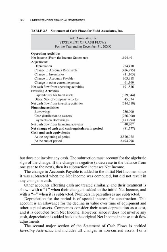
P1: OTA/XYZ P2: ABC



TABLE 2.3 Statement of Cash Flows for Fudd Associates, Inc.

Fudd Associates, Inc.STATEMENT OF CASH FLOWS

For the Year ending December 31, 20XX

Operating ActivitiesNet Income (From the Income Statement) 1,194,491Adjustments

Depreciation 234,410Change in Accounts Receivable (426,795)Change in Inventories (11,105)Change in Accounts Payable 303,918Change in other current expenses 91,399

Net cash flow from operating activities 191,826Investing Activities

Expenditures for fixed assets (359,344)Other: Sale of company vehicles 45,034

Net cash flow from investing activities (314,310)Financing activities

Borrowings 750,000Cash distribution to owners (236,000)Payments on Borrowings (473,294)

Net cash flow from financing activities 40,707Net change of cash and cash equivalents in period (81,777)Cash and cash equivalents:

At the beginning of period 2,576,075At the end of period 2,494,298

but does not involve any cash. The subtraction must account for the algebraicsign of the change. If the change is negative (a decrease in the balance fromone year to the next), then its subtraction increases Net Income.

The change in Accounts Payable is added to the initial Net Income, sinceit was subtracted when the Net Income was computed, but did not result inany change in cash.

Other accounts affecting cash are treated similarly, and their treatment isshown with a “+” when their change is added to the initial Net Income, andwith a “−” when it is subtracted. Numbers in parentheses are subtracted.

Depreciation for the period is of special interest for construction. Thisaccount is an allowance for the decline in value over time of equipment andother capital assets. Companies consider their asset depreciation as a cost,and it is deducted from Net Income. However, since it does not involve anycash, depreciation is added back to the original Net Income in these cash flowadjustments

The second major section of the Statement of Cash Flows is entitledInvesting Activities, and includes all changes in non-current assets. For a

P1: OTA/XYZ P2: ABC


CONTRACT BACKLOG 37

construction company, this section typically would include the purchase andselling of equipment and real estate. A company’s net income is not affectedwhen a company buys a new piece of equipment, since it is the even exchangeof one asset called cash for another asset called equipment (or the same in-crease in the asset called equipment and the liability called Accounts Payable,which does not change Net Income, either). However, the amount of availablecash is reduced by the purchase. The cost of all non-current assets purchasedin the analyzed period is included as a negative amount. The revenue fromselling any non-current asset, say a pickup truck, is added to this cash flowsubtotal.

The third and last section shown in Table 2.3 is Financing Activities. Anycash received from new loans is included here. This money increases the cashflow for the period. Conversely, loan payments are considered negative. Thissection also includes any issued company stock, which results in the infusionof new money and therefore, increases the cash flow. Cash distributions to thecompany owners reduce the availability of cash, and are shown as negativeamounts.

The algebraic addition of the three section subtotals is the Net Changein Cash and Cash Equivalents for the company during the period cov-ered by the Statement of Cash Flows. The Ending Cash Balance isfound by adding the Beginning cash balance to the computed Net changein cash.

CONTRACT BACKLOG

You may have noticed a problem with the financial statements that we havediscussed so far. If revenue includes only the value that the company hasalready generated during a specific period of time, then where do companiesplace the value of their contracts pending to be earned? This amount isreported as the contract backlog of the company. This is an important reportfor understanding the condition of a construction company going forward.A contractor may appear to be doing perfectly well so far, but if it has nobacklog, it will be in trouble in the immediate future.

This was the case of many homebuilders at the end of 2006. They hadexperienced an excellent market for years. However homebuilding construc-tion suffered a significant decline beginning in 2007. The lack of incomingcontracts should have been a red flag to investors that there might be troubleahead. The backlog can also indicate the opposite situation. A company’sresources may be overstretched if too many contracts are in the backlog.Adequate resources may not be available to support a rapidly increasing port-folio of projects. In this case, an over abundance of projects in the companybacklog would alert investors and lenders to the potential risk reflected bythis abnormal situation.

P1: OTA/XYZ P2: ABC



PUBLIC CORPORATIONS

A public corporation offers its shares for sale to the general public in a stockmarket such as the New York Stock Market or NASDAQ. Alternatively, acompany can organize as a privately held corporation. Stock in such compa-nies is not offered for sale or traded publicly.

Relatively few construction companies choose to organize as public cor-porations. The Federal Trade Commission (FTC) imposes strict report-ing requirements, so that potential investors have a clear picture of eachcompany’s financial position (and other management issues) before invest-ing in it. Among the many requirements for financial transparency, publiccompanies must formally report their financial position each quarter (i.e.,every three months) by submitting the FTC’s form 8-K, and filing an au-dited annual detailed report (10-K) with the FTC. Every major manage-ment event must be reported. These requirements are cumbersome by anystandard.

Almost always, public corporations begin as private entities which at onepoint decide to expand and open their stock to the general public in thestock market. The money from the sale of shares injects new capital into thecorporation, and consequently, enhances its ability to undertake expandedoperations.

The original shareholders of a private corporation which decides to “gopublic” have good financial incentives for the move. The first batch of pub-licly offered shares is called a corporation’s initial public offering (IPO).Investors may be willing to pay more than the face value (par value) of eachshare. This extra income is part of the owners’ equity, specifically under theaccount called Additional Paid-In Capital. The difference between the parvalue and what investors pay to the company for each share can be huge. Forexample, the par value of the first 19,605,052 shares of Google’s IPO was$0.001 (0.1 cent per share), and its selling value in the stock market was $85per share.

In addition to improving the cash position of the corporation, the originalshareholders can pocket extra money, sometimes becoming “instant million-aires,” when there is a difference in the price that they paid for their sharesand the price that the shares can command if they are sold in the stock market.Anyone who acquired Google stock at its IPO value made a very good deal,even if they paid $85 additional dollars per share. That person could havesold each share for $747 at the end of 2007. The down side is, of course, thatthis profit of $747 – $85 = $662 per share would be taxed as a capital gainfor the seller.

Public corporations must report their contract backlog as part of theirfilings to the FTC. A section of the 10-K is entitled Management’s Discussionand Analysis of Financial Condition and Results of Operation. This sectionprovides a table listing the reporting company’s projects under contract and

P1: OTA/XYZ P2: ABC



their earned and pending values. This table is obviously of interest to potentialinvestors.

Public companies also publish an annual report geared to investors. Theannual report presents a more attractive version of much of the informationgiven in the 10-K filing. It includes financial information regarding the pastyear’s performance with additional narrative highlighting the company’s ac-complishments. An annual report is an excellent source of information andit is designed to be easier to read than the austere format of Form 10-K. Itmust be kept in mind, however, that an annual report is designed to presentthe company in the best possible light. Negative factors must be reported (bystatute) but generally are not printed in big letters.

Privately held corporations do not have the reporting requirements of publiccorporations. Every company knows its backlog, but it is private informationnot available to the general public.


1. At the end of the fiscal year 20X2, Rainer Construction Co., Inc. has thefollowing financial profile (all figures are in dollars):

Total assets 1,200,000Total liabilities 850,000Total revenue before taxes 300,000Total expenses 265,000

(a) What is the total net worth of this company?(b) Did the net worth increase, decrease or remain the same compared to

FY 20X1? Why?(c) What is the income after taxes? (Assume a 50% tax rate.)

2. Define in your words the difference between a Balance Sheet and anIncome Statement.

3. The following Balance Sheet figures are available on the Cougar Con-struction Company:

Current Long-Term Total

Assets $100,000 $100,000 $200,000Liabilities 80,000 70,000 150,000

(a) Find the total net worth of the company.

P1: OTA/XYZ P2: ABC



4. The following data regarding Atlas Construction Company are available:

Current assets $300,000

Current liabilities 200,000Long-term liabilities 500,000Total net worth 200,000

What is the value of the company’s fixed assets?5. Name three accounts typical of the liability side of a Balance Sheet. In

what side would you enter “discounts earned?”6. How are the Balance Sheet and Income Statement related? Discuss the

pattern of information flow between these two documents.7. Given the data shown in Tables P2.7a and P2.7b for Pegasus Interna-

tional, Inc., what method of accounting is being used? How has theworking capital of Pegasus International changed from 20X4 to 20X5?Interpret this development considering the increase in revenue from20X4 to 20X5.

TABLE P2.7a Pegasus International, Inc., Summary of ConsolidatedOperations (Dollar Amounts and Shares Are in Thousands, Except Per ShareAmounts)

20X5 20X4

Revenue $1,325,423 $801,322Costs and expensesCost of revenue 1,211,402 726,937Corporate administrative and

general expenses19,392 14,881

Other (income) and expensesInterest on indebtedness 1,354 1,671Interest income −6,565 −7,089Provision for estimated losses on

planned disposition of assets— 400

Total cost and expenses 1,225,583 736,800Earnings before income taxes 99,480 64,522Total income taxes 52,429 31,277Net earnings 47,411 33,245Preferred dividend requirements 1,803 1,558Earnings applicable to common

stock$45,608 $31,687

P1: OTA/XYZ P2: ABC



TABLE P2.7b Pegasus International, Inc., Consolidated Balance Sheet

Assets 31 December, 20X5 and 20X4 20X5 20X4

Current assets Cash $10,138,000 $13,063,000Short-term investments at

cost, which approximatesmarket

101,310,000 49,298,000

Accounts and notes receivable 90,526,000 83,442,000Costs and earnings in excess

of billings on uncompletedcontracts

65,745,000 44,728,000

Inventories at lower of cost(average and FIFOmethods) or market

30,011,000 24,210,000

Other current assets 7,751,000 9,005,000

Total current assets 305,481,000 223,746,000Property, plant,and equipment at

Land

cost 11,162,000 11,744,000Buildings and improvements 39,622,000 26,909,000Machinery and equipment 50,650,000 51,597,000Drilling and marine

equipment107,617,000 71,300,000

Construction in process 42,834,000 44,230,000

Subtotal 251,885,000 205,780,000Less accumulated

depreciation andamortization

75,441,000 76,732,000

Net total property, plant, andequipment

176,444,000 129,048,000

Oil and gasproperties at cost

Subtotal 59,814,000 50,683,000

Less accumulated depletionand depreciation

30,455,000 20,105,000

Net total oil and gas properties 29,359,000 30,578,000Other assets Excess of cost over net assets

of acquired companies, lessaccumulated amortization

15,105,000 16,351,000

Other 12,058,000 12,542,000

Total other assets 27,163,000 28,893,000Total $538,447,000 $412,265,000

(continued )

P1: OTA/XYZ P2: ABC



TABLE P2.7b Pegasus International, Inc., Consolidated Balance Sheet (Continued )

Liabilities andShareholders’Equity 20X5 20X4

Current liabilities Accounts payable $66,050,000 $54,124,000Billings in excess of costs and

earnings on uncompletedcontracts

69,082,000 53,375,000

Accrued liabilities 58,089,000 37,393,000Current portion of long-term

debt1,395,000 1,385,000

Income taxes currentlypayable

24,895,000 8,209.00

Deferred income taxes 49,599,000 31,989,000

Total current liabilities 269,101,000 186,385,000Long-term debt

due after oneyear

Total 4,242,000 7,311,000

Other noncurrentliabilities

Deferred income taxes 11,623,000 11,792,000

Other 9,162,000 4,400,000Total $20,785,000 $16,192,000

Contingencies andCommitments

Shareholders’equity

Capital stock

Series B preferred $567,000 $663,000Common 9,368,000 9,203,000Additional capital 116,636,000

115,184,000Retained earnings 117,748,000 77,327,000

Total shareholders’ equity 244,319,000 202,377,000Total $538,447,000 $412,265,000

P1: OTA/XYZ P2: ABC


CHAPTER 3

ANALYZING COMPANYFINANCIAL DATA

INTRODUCTION

Every financial report tells something about a company’s financial health. Ifthe company reports a large profit, it may be a better investment than anotherthat reports a smaller profit. But which one is better also depends on otherfactors. If a company makes one million dollars in annual profit by performing100 million dollars of work, and another company can make a half a milliondollar profit on 25 million dollars of work, it would seem that the latter is amore attractive investment, since the first gets one cent in profit from eachdollar of work performed, while the second gets a five-cent profit on eachdollar of work performed.

The rationale above seems solid, but in fact it wouldn’t be wise to act basedsolely in the information provided so far. What if each company had the sameamount of owners’ equity, say five million dollars? From our perspective asinvestors, the first company now appears to be better: for each dollar invested,the first company gives a profit of 20 cents to the company’s owners, butthe second company gives only 10 cents on the dollar to the owners. Thedecision can get even more complicated. What if the second company hasbeen a quite consistent money maker over time, while the first one has had anerratic record, losing money in some years? Or if the second company has a50 million dollar bank note due in two years? Or if either company is makingless profit than its competitors? It is virtually impossible to judge the financialstatus of a company just by looking at its Balance Sheet, Income Statement,and other primary financial reports without some further point of reference.

This chapter addresses standard metrics, or indicators, for analyzing a set offinancial documents. These indicators greatly simplify the understanding of a

43



P1: OTA/XYZ P2: ABC


44 ANALYZING COMPANY FINANCIAL DATA

company’s financial status, since they consist of simple ratios and percentagesinstead of the many and large dollar amounts found in a typical financialstatements.

Vertical and Horizontal Analyses

There are many reasons for being interested in the financial status of a com-pany. Lenders and investors are particularly interested in determining the riskof losing the money that they are lending or investing, respectively, in thecompany. Sureties, labor unions, and even state and federal tax agencies alsoneed to understand a company’s financial health. All these parties have de-veloped ways to get a meaningful picture of a company’s finances using theprimary reports discussed in the previous chapters. These analysis procedurescan be grouped into two main categories, namely:

1. Vertical Analysis. A vertical analysis simplifies the interpretation offinancial information by developing a relatively small number of keyindicators from the numbers presented in a company’s Balance Sheetand Income Statement. This type of analysis takes its name from the factthat since it works with line items from financial statements, it usuallyrequires reading pages “from top to bottom.” The bulk of this chapterconcerns vertical analysis.

2. Horizontal Analysis. The purpose of a horizontal analysis is detectingthe direction and trends of key financial information. We can make muchmore sense of vertical analysis if we compare its results over a period oftime. Since time is normally shown graphically on the horizontal axis,this type of time-based analysis is called “horizontal.” As you will see,we can express these trends using their absolute values, or in proportionto an initial point in time. Notice that although different, vertical andhorizontal analyses do not exclude each other. Any good exploration ofthe significance of a company’s financial reports should include bothtypes of analyses if at all possible.

VERTICAL ANALYSIS: FINANCIAL RATIOS

Many financial indicators consist of ratios of items taken from the BalanceSheet and the Income Statement. These ratios provide clues and symptomsof undesirable conditions or highlight issues requiring further investigation.The analysis of an indicator can disclose relationships as well as bases forcomparison that reveal conditions and trends that cannot be properly detectedby reading the individual items in its formula.

Four main categories of ratios are commonly identified: Liquidity, Prof-itability, Efficiency and Capital Structure. Each one of these categories, in

P1: OTA/XYZ P2: ABC


LIQUIDITY INDICATORS: CAN THIS COMPANY GET CASH IN A HURRY? 45

turn, comprises several ratios. No company needs all possible indicators,since each industry has its own needs and preferences. For example, a com-mon indicator for a retailing business such as its inventory turnover may benear useless in construction. The reverse is also true; some common ratiosfor construction companies are rarely used in retailing. We will examine onlythe most common and useful ratios for a typical construction company. Theformula and explanation of many others are widely available and follow thesame rationale discussed here.

The numerical value of any ratio is in itself of limited value, since it doesnot furnish a context to understand the financial position of the company. Theratio becomes much more meaningful when it is combined with a horizontalanalysis, which shows its range and its trend over time. Furthermore, ratiosshould be compared with industry averages, which are published by the Con-struction Financial Management Association (CFMA), Standard and Poor’s,Robert Morris Associates and independent consultants. Most public librariescarry at least one of these sources.

LIQUIDITY INDICATORS: CAN THIS COMPANY GET CASHIN A HURRY?

Liquidity refers to the ability of a company to maintain a sound financialposition over the short term. In practical terms, good liquidity means that thecompany can pay its liabilities due in the relatively near future, usually withina year. In turn, paying off a liability requires cash. From a lender’s perspective,a company should have more cash and assets that can be easily converted tocash than the amount of liabilities that it needs to pay in the near future. Easilysellable assets are grouped as Current Assets; short-term liabilities are foundunder Current Liabilities. It follows that a company should have more currentassets than current liabilities.

We will look at three financial indicators that deal with the relative liquidityof a company, and are collectively known as Liquidity Indicators. The threeof them, namely the Current Ratio, Quick Ratio and Working Capital, addressa company’s liquidity by relating its Current Assets to its Current Liabilities.

Current Ratio

The Current Ratio can be visualized as the “safety factor” for a creditor’smoney loaned to a company, computed as the ratio between the total amountof Current Assets and Current Liabilities. Its formula is:

Current Ratio = Current Assets/Current Liabilities

When a company’s Current Ratio is greater than one, it means that thecompany has more cash, or assets easily convertible to cash, than the amount

P1: OTA/XYZ P2: ABC



TABLE 3.1 Current Ratio Computations for FuddAssociates, Inc

From the Balance SheetTotal current assets $12,880,550Total current liabilities $9,774,261

Current Ratio =Current Assets / Current Liabilities= $12,880,550 / $9,774,261 = 1.32

of money that it will have to pay in the near future. A lender wants this ratioto be as large as possible.

The typical desirable range for a construction company’s Current Ratio isbetween 1.5 and 3.0. A value of less than 1.5 means that the company maystruggle to find enough cash or easily convertible assets to pay its currentliabilities. The reason for an upper limit for this and other financial indicatorsis more subtle. An unusually large Current Ratio may indicate an excessivelyconservative management—which is not desirable.

Table 3.1 shows the current ratio computations for Fudd Associates, Inc.The Balance Sheet and Income Statement used for these computations, as wellas for the others in the remainder of this chapter, are taken from Tables 2.1and 2.2.

The average Current Ratio of most construction companies, even thosesoundly managed is low compared to the usually acceptable range for otherindustries. In most industries, a Current Ratio of less than 2.0 raises a red flagwith lenders. Construction is a risky line of business, and its relatively lowindustry averages reflect this fact. Moreover, most contractors have minimalamounts of inventory, relying instead on a pretty tight supply chain from theirsubcontractors and material suppliers. The larger Current Ratio averages forother industries derive in part from their larger inventories and a much higherproportion of their business done with in-house resources.

Quick Ratio

The Quick Ratio’s rationale and computation are very similar to the CurrentRatio’s, with the difference that the Quick Ratio is more stringent than theCurrent Ratio. Its formula is:

Quick Ratio = (Near-cash Current Assets)∗/Current Liabilities

The Quick Ratio has exactly the same denominator of the Current Ra-tio, namely the company’s Current Liabilities. In the numerator, it also has

∗ Near-Cash = Easily liquidable

P1: OTA/XYZ P2: ABC


LIQUIDITY INDICATORS: CAN THIS COMPANY GET CASH IN A HURRY? 47

TABLE 3.2 Quick Ratio Computations for Fudd Associates, Inc.

From the Balance SheetCurrent near-cash assets (above Inventories)

Cash and cash equivalents $2,494,298Account receivables $8,535,901Costs & recog’d earnings in excess of billings $933,165

Total current near-cash assets $11,963,364Total current liabilities $9,774,261

Quick Ratio =Current near-cash assets / Current Liabilities= $11,963,364 / $9,774,261 = 1.22

accounts from Current Assets, with the difference that it uses only the mostliquid (easily convertible to cash) of the Current Assets accounts as opposedto the Current Ratio, which includes all Current Assets in its formula.

The near-cash current assets considered by the Quick Ratio are, morespecifically, all those listed above the Inventories account (not includingInventories). The accounts in the Current Assets section of a Balance Sheet arelisted in order of liquidity, beginning with Cash itself. Although Inventories isa Current Assets account, it is not as easily liquidable as Cash (the account) andnear-cash accounts such as Accounts Receivable. Should a company declarebankruptcy, its inventories could be difficult to sell, and even harder to price.

Since the Quick Ratio includes only the most liquid Current Assets in thenumerator, its value will always be less than the Current Ratio of the samecompany. The Quick Ratio is also called the Acid Ratio because like acid, itis “corrosive” (more demanding) than the Current Ratio. Table 3.2 shows theQuick Ratio computations for Fudd Associates, Inc.

The standard recommended range for Quick Ratio is between 1.0 and 2.0.Construction companies tend to have quite good Quick Ratios. The smallamount of inventory carried by most construction contractors makes theirCurrent and Quick Ratios numerically close, and consequently, althoughtheir Current Ratio is low as previously discussed, their Quick Ratio is highcompared to typical retailers’ and manufacturers’.

Working Capital

The Working Capital indicator and the Current Ratio use exactly the same in-formation in their formulas, but instead of dividing Current Assets by CurrentLiabilities, Working Capital subtracts the balances of these accounts:

Working Capital = Current Assets − Current Liabilities

This indicator shows the dollars that a company could use to increaseits business. Any leftover of Current Assets minus Current Liabilities is in

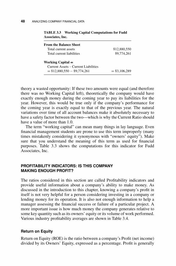
P1: OTA/XYZ P2: ABC



TABLE 3.3 Working Capital Computations for FuddAssociates, Inc.

From the Balance SheetTotal current assets $12,880,550Total current liabilities $9,774,261

Working Capital =Current Assets – Current Liabilities= $12,880,550 − $9,774,261 = $3,106,289

theory a wasted opportunity: If these two amounts were equal (and thereforethere was no Working Capital left), theoretically the company would haveexactly enough money during the coming year to pay its liabilities for theyear. However, this would be true only if the company’s performance forthe coming year is exactly equal to that of the previous year. The naturalvariations over time of all account balances make it absolutely necessary tohave a safety factor between the two—which is why the Current Ratio shouldhave a value of more than 1.0.

The term “working capital” can mean many things in lay language. Evenfinancial management students are prone to use this term improperly (manytimes mistakenly considering it synonymous with “owners’ equity”). Makesure that you understand the meaning of this term as used for financialpurposes. Table 3.3 shows the computations for this indicator for FuddAssociates, Inc.

PROFITABILITY INDICATORS: IS THIS COMPANYMAKING ENOUGH PROFIT?

The ratios considered in this section are called Profitability indicators andprovide useful information about a company’s ability to make money. Asdiscussed in the introduction to this chapter, knowing a company’s profit initself is not very helpful for a person considering investing in a company orlending money for its operation. It is also not enough information to help amanager assessing the financial success or failure of a particular project. Amore important issue is how much money the company generates relative tosome key quantity such as its owners’ equity or its volume of work performed.Various industry profitability averages are shown in Table 3.4.

Return on Equity

Return on Equity (ROE) is the ratio between a company’s Profit (net income)divided by its Owners’ Equity, expressed as a percentage. Profit is generally

P1: OTA/XYZ P2: ABC


TA

BL

E3.

4Sa

mpl

eIn

dust

ryP

rofit

abili

tyR

atio

s—

Bas

edon

IRS

Ret

urn

Info

rmat

ion

Com

pute

ran

dM

otor

Veh

icle

sC

onst

ruct

ion

ofPe

riph

eral

and

Part

sN

ewan

dU

sed

Indu

stry

Bui

ldin

gsE

quip

men

tM

anuf

actu

rers

Gas

olin

eSt

atio

nsC

arD

eale

rsA

ccom

mod

atio

n

NA

ICS

(Ind

ustr

yId

entifi

er)

2361

1533

4110

3361

0544

7100

4411

1572

1115

Ret

urn

onTo

talA

sset

s8.

1%8.

1%2.

5%5.

8%5.

1%3.

5%R

etur

non

Equ

itybe

fore

Inco

me

Taxe

s26

.2%

16.8

%1.

0%11

.1%

16.0

%0.

3%R

etur

non

Equ

ityaf

ter

Inco

me

Taxe

s21

.7%

10.3

%0.

2%9.

5%14

.2%

—R

etur

non

Rev

enue

befo

reIn

com

eTa

xes

3.7%

7.6%

0.4%

0.7%

0.9%

0.2%

Ret

urn

onR

even

ueaf

ter

Inco

me

Taxe

s3.

0%4.

7%0.

1%0.

6%0.

8%—

©20

07L

eoT

roy

-A

lman

acof

Bus

ines

san

dIn

dust

rial

Fin

anci

alR

atio

s,20

07E

ditio

n

49

P1: OTA/XYZ P2: ABC



TABLE 3.5 Return on Equity Computations for FuddAssociates, Inc.

(Net Worth = Owners’ Equity)From the Balance Sheet

Total net worth $4,732,935

From the Income StatementNet Income $1,194,491

Return on Equity =Net Income / Total Owner’s Equity= $1,194,491 / $4,732,935 = 0.2524 or 25.24%

considered here as the profit remaining after paying taxes but before payingdividends to owners. The formula for this indicator is:

Return on Equity = Profit/Owners’ Equity

For an investor considering whether a particular company is a good invest-ment, its ROE is usually the deal maker or breaker. ROE can be visualized asthe interest that the investor gets on his money. If the company shows a 10%ROE, it means that the investor gets a 10 cents profit in one year for eachdollar invested. If a totally similar company has an ROE of, say, 12%, theinvestor would probably opt for the latter, unless noneconomic factors play amajor role in the decision.

Table 3.5 shows the ROE computations for Fudd Associates, Inc.There are many factors to consider other than ROE when investing op-

portunities do not refer to comparable business schemes. If a bank offers a10% return on certificates of deposit, most investors would choose this op-tion over investing in a construction company with a 10% ROE, since thebank’s offer is much less risky than the option of investing in a constructioncompany. The higher risk of investing in construction companies may be wellrewarded. The average ROE for construction compares favorably to manyother industries. The management quality of an individual company heavilyinfluences its ROE. For example, Robert Morris Associates (RMA) AnnualStudies (2007) shows that Industrial Building Construction contractors havean average ROE of 25.5%. However, the top quartile earns 46.4%, and thebottom quartile earns 5.9%, a quite significant difference.

Return on Revenue

Return on Revenue (ROR) indicates how many cents of profit a contractor isgetting from each dollar of revenue. The formula for this ratio is, therefore:

Return on Revenue = Profit/Revenue

P1: OTA/XYZ P2: ABC


PROFITABILITY INDICATORS: IS THIS COMPANY MAKING ENOUGH PROFIT? 51

TABLE 3.6 Return on Revenue Computations for FuddAssociates, Inc.

From the Income StatementNet Income $1,194,491Total Revenue $45,226,102

Return on Revenue =Net Income / Total Revenue= $1,194,491 / $45,226,102 = 0.0264 or 2.64%

The ROR computations for Fudd Associates, Inc. are shown in Table 3.6.ROR is most interesting to internal managers, while ROE is crucial for

investors and creditors. Since profit and revenue can be tracked for eachindividual project, ROR can tell the profitability of each one. For individualproject managers, ROR can have a great personal impact. A manager whoseprojects have a high ROR is likely to get a higher bonus than another managerwith lower project ROR, if their projects are comparable.

Construction companies have a relatively low ROR compared to otherindustries, as you can see in Table 3.6. However, construction contractors canperform very large projects with little capital of their own. This makes thedenominator in the ROR formula comparatively large and, therefore, the RORcomparatively low. The low ROR construction company average does indicatean intrinsic problem of the industry—just a few cents’ difference between theestimated and actual project unit costs makes the difference between a profitor a loss. The business of construction is, indeed, risky.

Return on Assets

A company’s Return on Assets (ROA) is computed similarly to its ROEand ROR:

Return on Assets = Profit/Total Assets

If a company is considering borrowing money, its ROA provides a veryuseful control value. If the money will be borrowed at an interest rate belowthe company’s ROA, then the company will make a profit from taking theloan. If the loan requires paying a greater interest than the company’s ROA,then the loan should not be taken, because the company will pay more in totalinterest than the profit it can realize. The ROA for Fudd Associates, Inc. isshown in Table 3.7.

Earnings Per Share

A corporation keeps track of its Earnings per Share (EPS). Its formula is:

Earnings per Share = Profit/Company stock shares

P1: OTA/XYZ P2: ABC



TABLE 3.7 Return on Assets Computations for FuddAssociates, Inc.

From the Income StatementNet Income $1,194,491

From the Balance SheetTotal Assets $15,978,849

Return on Assets =Net Income / Total Assets= $1,194,491 / $15,978,849 = 0.0748 or 7.48%

The profit, as in the previous cases, normally refers to the net income aftertaxes. The company stock shares refers, more precisely, to the average numberof shares of common stock outstanding.1

If a company makes a profit of $50 million for the year and has 40 millionshares of common stock in circulation, then its EPS will be 50/40 = $1.25per share. A shareholder owning 10,000 shares of common stock can easilyfigure that her investment in this company resulted in an individual profit of$12,500 for the year.

Public corporations report their EPS quarterly. This indicator is themost closely watched by public corporation shareholders. Few construc-tion companies are incorporated as public corporations. The exceptionsare real estate developers, which need large amounts of money for theiroperation and frequently take advantage of the influx of cash resultingfrom offering their stock in stock markets such as the New York StockExchange (NYSE).

EFFICIENCY INDICATORS: HOW LONG DOES IT TAKE A COMPANYTO TURN OVER ITS MONEY?

The indicators under the category of Efficiency consider the time that acompany needs to circulate the money it has, owes or is owed. Since thismoney circulation is the essential activity of any company (a company is a“money pump”), these statistical measures are also called Activity Indicators.The unit for the indicators discussed here is time, usually expressed in days,or cycle times per year.

1 The number of shares can vary during the period reported by the EPS, and, therefore, the number ofshares for the period must be averaged. Moreover, there can be several types of shares, such as preferredstock and common stock. Outstanding stock is the number of shares actually held by shareholders.

P1: OTA/XYZ P2: ABC


EFFICIENCY INDICATORS: HOW LONG DOES IT TAKE A COMPANY TO TURN OVER ITS MONEY? 53

The rationale for the formulas of ratios in this category is pretty straight-forward, as the following two examples show.

A) Suppose that a car has traveled a total of 24,000 miles last year, and theaverage trip was 2,000 miles long. How long did it take on average tocomplete each trip? The answer is:

2,000 miles / 24,000 miles per year = 0.08333 years,or in months, 0.08333 × 12 = 1.0 months,or in days, 0.08333 × 365 = 30.4 days.

B) Suppose that you have spent a total of $24,000 in materials last year, andthe average inventory of materials was $2,000. How long did it take onaverage to deplete your inventory? The answer is:

$2,000 / $24,000 per year = 0.08333 years,or in months, 0.08333 × 12 = 1.0 months,or in days, 0.08333 × 365 = 30.4 days.

As you can see, the two examples above are virtually identical; the onlydifference being that the first one deals with distance and the second one withmoney. You can also approach the second example from a different angle.The inventory was depleted 12 times in the year ($24,000 per year / $2,000).Therefore, it took 1/12 of a year, or one month, or 30.4 days, to deplete orturn-over the inventory.

Table 3.8 shows the average ages for several construction specialties foritems discussed below.

Average Age of Inventory

This indicator was introduced in the preceding example. The formula thatfollows formalizes the concept.

Average Age of Inventory

= (Average Inventory Balance/Total Cost of Inventory) × 365

TABLE 3.8 Important Average Ages for the Construction Industry (in days)

Industrial and Heavy andSpecialty All Companies Nonresidential Highway Specialty Trade

Days in Acct. Receivable 51.4 48.4 45.5 67.7Days in Inventory 3.2 0.2 3.8 2.6Days in Acct. Payable 41 46.8 34.7 29.2Operating Cycle 31.5 22.1 37.2 49.6

© 2007 Construction Financial Management Association in RMA Annual Statement Studies

P1: OTA/XYZ P2: ABC



The Average Inventory Balance is found by averaging the balance forthe Balance Sheet account called Inventory as many times as possible overthe period covered by the Income Statement. If this period is one year, theAverage Inventory Balance could be found by averaging out the balancesof the Inventory account at the end of each quarter: March 31, June 30,September 30, and December 31.

The denominator of the formula comes from the Income Statement, whichcontains an account called Cost of Inventories. This account shows the costof the entire inventory purchased in the year. It is the equivalent of the totalmileage in the first example above. Finally, the 365 in the formula comesfrom the days in a year. If the Income Statement covered a semester, theninstead of 365 we would use 180, the days usually assumed for one half year.These steps can be seen in Table 3.9, which consists of the computations ofthe Average Age of Inventory for Fudd Associates, Inc.

Materials and parts required for a project are kept in inventory, on average,for the number of days shown by this indicator. Having parts sitting idle in thewarehouse is not necessarily bad, since the more parts are available, the lesslikely it is that the project will stop for lack of materials or parts. However,a company’s inventory is not generating any money. On the contrary, thecompany may be paying interest if it was purchased on credit.

As previously mentioned, most construction contractors don’t keep largeinventories, and this indicator is not as critical in the construction industry asmost of the others discussed here. Some specialties do keep sizable inventoriesand should pay close attention to their Average Age of Inventory. Largehomebuilders maintain large inventories (since they tend to provide materialsto their subcontractors). Specialty contractors such as electrical contractingcompanies also maintain large inventories.

TABLE 3.9 Average Age of Inventory Computations for FuddAssociates, Inc.

From the four most recent quarterly Balance SheetsInventory at 3/31/XX $139,788Inventory at 6/30/XX $91,899Inventory at 9/30/XX $115,550Inventory at 12/31/XX $122,106

Average Inventory $117,336

From the Income Statement(Assuming Cost of Inventory = Cost of Materials)

Cost of Inventory $9,563,314

Average Age of Inventory =(Average Inventory / Cost of Inventory) × 365= ($117,336 / $9,563,314) × 365 = 4.5 days

P1: OTA/XYZ P2: ABC



The average age of inventory is important to manufacturing companies thatfabricate products and hold them in inventory prior to sale. This is not the waythe construction of a project proceeds. We do not say that the work completedto date on a project is held in inventory. Therefore, inventory-based ratios arenot as directly applicable in construction as in the manufacturing sector.

Average Age of Accounts Receivable (Collection Period)

The rationale for the Average Age of Accounts Receivable is conceptuallysimilar to the previous examples. Revenue is our “total mileage” for thisindicator because for practical purposes, in construction all the revenue isfirst billed and then collected.

If the Income Statement covers one year, the formula for this indicator is:

Average Age of Accounts Receivable

= (Average balance of Accounts Receivable/Revenue) × 365

As in the previous case, if the Income Statement does not summarize ayear of operations, the 365 would be replaced by the number of days of theperiod covered by the Income Statement.

The computations for Fudd Associates, Inc. shown in Table 3.10 can helpin understanding these computations.

Keeping a short collection period is of utmost importance to any construc-tion company. A company can be rich in assets, and yet go bankrupt if it haslarge balances of Accounts Receivable but no cash to pay its immediate obli-gations. Construction companies are at constant risk of exhausting their cashreserves due to the standard contract payment terms and the large amount ofsubcontracted work on a typical job.

TABLE 3.10 Average Age of Accounts ReceivableComputations for Fudd Associates, Inc

From the four most recent quarterly Balance SheetsA/R at 3/31/XX $6,588,333A/R at 6/30/XX $5,375,100A/R at 9/30/XX $6,590,000

A/R at 12/31/XX $8,635,901Average A/R $6,797,334

From the Income StatementTotal Revenue $45,226,102

Average Age of Accounts Receivable =(Average A/R / Total revenue) × 365= $(6,797,334 / $45,226,102) × 365 = 54.9 days

P1: OTA/XYZ P2: ABC



Average Age of Accounts Payable

The same approach used for the average ages of Inventory and AccountsReceivable is applicable here once more. The formula for this indicator is:

Average Age of Accounts Payable

= [Average balance of Accounts Payable/

(Direct Costs − Cost of Labor)] × 365

As before, an average balance for the Accounts Payable must be computedfor the analyzed period. The 365 is replaced by the number of days coveredby the Income Statement if the period is not one year.

The denominator in the above formula is a bit different from the previousindicators because the equivalent of “total miles” discussed on the exampleat the beginning of this section is not as straightforward. The majority ofpurchases for any project are initially posted as Accounts Payable, since theyare purchased on credit and later paid off. The big exception to this rule is thecost of labor, which normally doesn’t pass through Accounts Payable since itis paid virtually as soon as it is incurred. To compare apples to apples, then, thecost of labor must be deducted from the total Direct Cost. If a project has otheraccounts paid on a cash (non-credit) basis, they should be subtracted as well.Table 3.11 consists of the Average Age of Accounts Payable computationsfor Fudd Associates, Inc.

The practical effect of the Average Age of Accounts Payable is the oppositeto its Accounts Receivable counterpart. The more you delay paying a debt,the more money you have to operate your company.

TABLE 3.11 Average Age of Accounts Payable for FuddAssociates, Inc.

From the four most recent quarterly Balance SheetsA/P at 3/31/XX $4,546,338A/P at 6/30/XX $2,786,200A/P at 9/30/XX $4,300,290A/P at 12/31/XX $3,659,156

Average A/P $3,822,996

From the Income StatementDirect costs $41,476,336Labor Costs $4,974,871

Average Age of Accounts Payable =(Average A/P / (Direct costs − labor costs)) × 365= ($3,822,996 / ($41,476,336 − $4,974,871)) × 365 = 38.2 days

P1: OTA/XYZ P2: ABC



TABLE 3.12 Average Age of Underbillings for FuddAssociates, Inc.

From previous Balance Sheets (not shown)Average Underbillings $937,486


Average age of Underbillings =(Average Underbillings / Total revenue) × 365= ($937,486 / $45,226,102) × 365 = 7.6 days

Other Average Ages

The computation of average ages for Costs and Estimated Profit in Excess ofBillings (Underbillings) and Billings in Excess of Costs and Estimated Profit(Overbillings) follow a similar logic, resulting in similar formulas, as you cansee in Table 3.12 and Table 3.13.

Similar to previous examples, the average amounts for Fudd’s Under-billings and Overbillings were computed as the simple average of the respec-tive balances for these Balance Sheet accounts at the end of each quarter. Theamount of Revenue, as in previous examples, comes from Fudd’s IncomeStatement.

Operating Cycle

What happens to a dollar invested in a construction project? As shown in Fig-ure 3.1, the dollar sits on each of the arrows for the number of days found foreach indicator in the Efficiency category, either increasing the time that it takesfor the dollar to come back to us (Inventory, Underbillings, and Accounts Re-ceivable) or decreasing this time (Underbillings and Accounts Payable). Thistotal time is called the company’s operating cycle, usually expressed in days.

TABLE 3.13 Average Age of Overbillings for Fudd Associates, Inc.

From previous Balance Sheets (not shown)Average Overbillings $742,820


Average age of Overbillings =(Average Overbillings / Total revenue) × 365= ($742,820 / $45,226,102) × 365 = 6.0 days

P1: OTA/XYZ P2: ABC



Inventory Accounts Receivable Under- billings

Accounts Payable Over- billings

Operating Cycle

Avg.Agei Avg.Ageub Avg.Agear

Avg.Ageap Avg.Ageob

Figure 3.1 Operating cycle.

Turnover Ratios

Although the use of average ages is very common in construction, otherindustries tend to use the inverse of the average ages computed in this section.These inverse amounts are called Turnover Ratios, and show how many timesin a year a company cycles its inventories, accounts receivable, or any otherof the items discussed in this section. Accounts Receivable Turnover, forexample, is the inverse of the Average Age of Accounts Receivable. If thisage is expressed in years (say 0.10 years), then its turnover is simply itsnumerical inverse (1/0.10 = 10.0 times per year). If the age is in days, then aconversion is needed, as shown in the following example.

A company has an average age of inventory of 30.4 days. The inventoryturnover for this company is:

(365 days in a year)/(30.4 days) = 12.0 times/year

An inventory turnover of 12.0 times per year means that the company’sinventory was used up and replenished 12 times.

Some ratios are customarily computed as turnovers and virtually never asaverage ages. They have the same conceptual framework as the previouslydiscussed turnovers. They show how many times an item has been leveraged(i.e., multiplied) compared to another during the period covered by the IncomeStatement.

Revenue to Assets Turnover

One ratio that is frequently expressed as a turnover instead of as an averageage is the Revenue to Total Assets Turnover. It indicates how much annualvolume of work a company did compared to its Total Assets. A large value

P1: OTA/XYZ P2: ABC


CAPITAL STRUCTURE INDICATORS: HOW COMMITTED ARE THE OWNERS? 59

TABLE 3.14 Revenue to Assets Turnover for FuddAssociates, Inc.

From the Balance SheetTotal Assets $15,978,849


Revenue to Assets turnover =Total Revenue / Total Assets= $45,226,102 / $15,978,849 = 2.83

for this ratio is desirable to the company owners but implies added risk topotential creditors. Its formula is:

Revenue to Assets Turnover = Revenue/Total Assets

Table 3.14 shows the computations of this indicator for Fudd Asso-ciates, Inc.

CAPITAL STRUCTURE INDICATORS: HOW COMMITTEDARE THE OWNERS?

The final indicator category that we will address here is called Capital Struc-ture. It addresses the relative size of a company’s assets, liabilities, and own-ers’ equity. The indicators in this category are useful for internal managersbecause they show whether the company is borrowing too much money com-pared to the amount of its total assets and owner’s equity. That is, is thecompany overinvested?

Investors and creditors may stay away from a construction company thathas borrowed, for example, 10 million dollars and whose owners have a totalequity of, say, half a million dollars. To understand the rationale here, comparesuch a company with another that has borrowed the same dollar amount butwhose owners have five million dollars of equity in the company. Should afinancial crisis arise, two very negative things can happen in the case of thefirst company. First, since all creditors must be paid off by liquidating thecompany’s assets, there would be a real possibility that the proceedings ofthe sale plus the company’s owners’ equity would not be enough to pay allliabilities. Second, owners would have little incentive to remain in businessduring the crisis, and could just “cut and run” with a small personal losscompared to the amount of trouble they might incur. In the case of the secondcompany, creditors would have to count less on the money generated by thesale of assets to get paid, and the company owners would think twice before

P1: OTA/XYZ P2: ABC



TABLE 3.15 Debt to Equity for Construction Specialties

All Industrial and Heavy and SpecialtySpecialty Companies Nonresidential Highway Trade

Debt to Equity 2.5 3.8 1.4 1.7

© 2007 Construction Financial Management Association

leaving behind the company and its creditors. They would stand to lose moreof their $5 million equity stake.

Debt to Equity

The term debt as used here is synonymous with Total Liabilities (whichis admittedly confusing). The Debt to Equity ratio, therefore, shows therelation of a company’s Total Liabilities compared to its Owners’ Equity.The introductory discussion for this ratio category in the previous paragraphsimplicitly pointed out the importance of this indicator, since it establishes howcommitted the owners are to their company. The formula for this ratio is:

Debt to Equity = Total Liabilities/Total Owners’ Equity

The higher the value of a company’s Debt to Equity, the riskier the companyis in the eyes of potential creditors. Table 3.15 compares this ratio acrossseveral construction specialties.

Assets to Equity (Leverage)

Instead of using Debt to Equity, some companies use the Assets to Equityratio, which is also called Leverage or Gearing. This formula is:

Assets to Equity (Leverage) = Total Assets/Total Owners’ Equity Leverage

Debt to Equity and Assets to Equity are related as follows:

Assets to Equity (Leverage) = Debt to Equity + 1

Table 3.16 gives a brief proof of this relationship.Table 3.17 shows the computation of this ratio for Fudd Associates, Inc.,

which numerically checks with the above equation.

OTHER INDICATORS

As mentioned in the introduction to this chapter, there are dozens of financialindicators, each one being of more relevance to some industries than to others.

P1: OTA/XYZ P2: ABC


OTHER INDICATORS 61

TABLE 3.16 Proof of Assets to Equity = Debt to Equity + 1

Assets to Equity = Total Assets / Owners’ Equity ①But, Total Assets = Total Liabilities + Owners’ Equity ②Replacing Total Assets in ①,Assets to Equity = (Total Liabilities + Owners’ Equity) / Owners’ Equity ③Distributing the denominator,Assets to Equity = (Total Liabilities / Owners’ Equity)

+ (Owners’ Equity / Owners’ Equity) ④Since Debt to Equity = Total Liabilities / Owners’ Equity ⑤and Owners’ Equity / Owners’ Equity = 1 ⑥

Assets to Equity = (Debt to Equity) + 1 ⑦

One indicator of particular importance for heavy/highway contractors relatesto the quality of assets.

This indicator provides a rough idea of how new or depleted a companyequipment fleet is, by dividing the depreciated value of the equipment by itspurchase value. A value close to one indicates a newer (nondepreciated) fleet.The formula for this indicator is:

Asset Newness

= (Purchase Value − Accumulated Depreciation)/Purchase Value

As the formula implies, this indicator varies from 1.0 for a totally new fleetto 0.0 to a completely depreciated one. Although values in between thesetwo extremes provide an idea of a fleet’s age, it is not intended to accuratelyreflect its maintenance and condition. Accounting practices do not considerthe market value of any asset, and, therefore, the book value of any piece ofequipment (purchase value minus accumulated depreciation) is only a crudeapproximation of its practical worth. Table 3.18 shows the computations forthe asset newness of Fudd Associates, Inc.

TABLE 3.17 Assets to Equity Computations for FuddAssociates, Inc.

From the Balance SheetTotal Assets $15,978,849Total Owners’ Equity $4,732,935

Assets to Equity =Total Assets / Total Owners’ Equity= $15,978,849 / $4,732,935 = 3.38

P1: OTA/XYZ P2: ABC



TABLE 3.18 Asset Newness Computations for Fudd Associates, Inc.

From the Balance Sheet(PP&E = Property, Plant and Equipment)

PP&E purchase cost $4,261,559PP&E Accum. Depreciation $(2,344,097)

$1,917,462Asset Newness =(PP&E purchase cost) − (PP&E Accum. Depreciation)

PP&E purchase cost

= $1,917,462

$4,261,559= 0.45

HORIZONTAL ANALYSIS: TRACKING FINANCIAL TRENDS

A critical factor revealed by comparative financial statements is trend. Track-ing how the numerical value of a financial item such as Return on Equityor Accounts Receivable has changed over time provides information regard-ing the performance of a company. As previously mentioned, this type ofanalysis is called “horizontal” analysis since the parameters of interest areplotted against time and time is usually shown on the horizontal axis. We willconsider two types of graphs used in a horizontal financial analysis: TimeSeries and Index-Number Trend Series.

TIME SERIES GRAPHS

A comparison of the value of a financial item over a number of years canreveal much about its direction (improving or worsening), its velocity (fastor slow), and its amplitude (large or small). This graph is more revealingand easier to understand than any narrative, and shows this information in anextremely compact way. Figure 3.2 shows the trend of the Return on Equity

25%

20%

15%

10%

Ret

urn

On

Equ

ity

5%

0%1998 2000 2002 2004 2006 2008

Figure 3.2 Fudd, Inc. Return on Equity for the past 10 years.

P1: OTA/XYZ P2: ABC


CONCLUSION 63

1200

1000

800

600

400

200

1985

Brid

ge C

ost I

ndex

20052000

1967 Base Index

1995199019801975197019650

x xxxxxxxx xx xx

x xx x x x xxx xx x x x

xxx x

x

xx x

xxxxxxx

Figure 3.3 Index series for bridge construction in California.

for Fudd Associates, Inc. You can readily appreciate not only that Uncle Fuddhas been successful in keeping an acceptable ROE, but that it has improvedover time.

Index-Number Trend Series

When a comparison of financial statements is made over a longer multiyearperiod, a year-to-year numerical assessment such as the side-by-side com-parison becomes cumbersome. The best way to perform such longer-termcomparisons is by means of index numbers. A year’s index number is simplythe ratio between the value analyzed for that year and a reference year calledthe base year.

Figure 3.3 consists of the indexes for the cost of bridge construction inCalifornia from 1967 to 2007. In this particular series, 1967 is assigneda value of 100, and the number in each following years is computed bycomparing the cost of building the same bridge in the year with its cost in1967. The index for 2007 is 960. This means that the standard bridge used forthe index costs 960/100 = 9.6 times more in 2007 than in 1967. The indexfor 1987 is 441, which means that it would cost 960/441 = 2.18 times to buildthe same bridge in 2007 compared to 1987.

CONCLUSION

Financial indicators and all techniques developed to gain insight into a com-pany’s financial health are empirical by nature. They are the result of dis-tilling from a company’s Balance Sheet and Income Statement a compactrepresentation of the company’s performance and value. Anyone can in-vent a new indicator, as is the case of private financial analysts (e.g., theFails Management Institute), who keep track of unconventional statistics that

P1: OTA/XYZ P2: ABC



they have found to be useful for their practice. For example, a companycould calculate the ratio between its Total Revenue and its number of su-perintendents. This metric could be used to assess whether the companyhas too few superintendents for its current revenue, or vice versa, if it hastoo many.

We have considered a number of financial indicators in this chapter, andyet they are but a fraction of the metrics available to a company. For exam-ple, some companies compute their revenue to fixed assets ratio and theirbook value per share (total owners’ equity/common shares outstanding).These ratios are important for manufacturing plants and public corporations,respectively, and could be included in a construction financial managementtext. But, inevitably, a selection must be made of the most useful indicators.The reader is encouraged to investigate and even create additional metricsthat could be valuable for their particular case.


1. Name and discuss four principal tools of financial analysis.2. Give two examples of an activity ratio. What do these ratios reflect?3. Analyze the operations of the Jumbo Construction Company across a

five-year period based on the data in Table P3.1.(a) Plotting significant times and ratios of your choice aid in your anal-

ysis. What is your assessment of the financial health of Jumbo Con-struction?

4. Given the balance sheet in Table P3.2, calculate the following ratios:(a) Current ratio(b) Quick ratio(c) Debt-equity ratio

5. How does trend analysis supplement the basic financial ratio calculationsand their interpretation?

6. Given a current ratio of 1.7, to which percentage of book value would youhave to liquidate current assets to be able to pay off current liabilities?

7. Given that the current ratio (i.e., current assets/current liabilities) for acompany over the years is as shown, what can you say about the operationof this company?

20X1 20X2 20X3 20X4 20X51.50 1.51 1.42 1.20 0.95

P1: OTA/XYZ P2: ABC


TA

BL

EP

3.1

Jum

boC

onst

ruct

ion

Com

pany

Fiv

e-Y

ear

Con

solid

ated

Sum

mar

yof

Ope

rati

ons

20X

520

X4

20X

320

X2

20X

1

Rev

enue

s$8

32,4

20,0

00$3

91,2

36,0

00$1

82,6

84,0

00$2

14,9

73,0

00$4

62,8

22,0

00In

tere

stan

ddi

vide

ndin

com

e2,

526,

000

3,80

2,00

02,

627,

000

1,30

4,00

01,

005,

000

Cos

tof

cont

ract

s77

5,55

2,00

034

7,42

5,00

014

8,84

6,00

018

3,86

2,00

043

4,12

0,00

0G

&A

expe

nses

36,1

29,0

0035

,100

,000

29,2

07,0

0026

,676

,000

23,2

20,0

00In

tere

stex

pens

e2,

199,

000

1,08

9,00

0—

——

Inco

me

befo

reta

xes

21,0

66,0

0011

,424

,000

7,25

8,00

05,

739,

000

6,48

7,00

0Pr

ovis

ion

for

inco

me

taxe

s10

,700

,000

5,70

0,00

03,

600,

000

2,80

0,00

03,

500,

000

Net

inco

me

12,6

66,0

005,

724,

000

3,65

8,00

02,

939,

000

2,98

7,00

0N

etin

com

epe

rsh

are

5.51

2.51

1.62

1.31

1.34

Div

iden

dspe

rsh

are

.70

0.45

0.35

0.33

Ave

rage

num

ber

shar

es2,

298,

000

2,28

1,00

02,

252,

000

2,23

6,00

02,

230,

000

65

P1: OTA/XYZ P2: ABC


TA

BL

EP

3.2

Bal

ance

Shee

t,C

yclo

neC

onst

ruct

ion

Co.

(31

Dec

embe

r20

12)

Ass

ets

Lia

bilit

ies

(a)

Cur

rent

asse

ts(f

)C

urre

ntlia

bilit

ies

Cas

hon

hand

and

onde

posi

t$3

89,9

27.0

4A

ccou

nts

paya

ble

$306

,820

.29

Not

esre

ceiv

able

,cur

rent

-16

,629

.39

Due

subc

ontr

acto

rs71

3,99

1.66

Acc

ount

sre

ceiv

able

,inc

ludi

ngA

ccru

edex

pens

esan

dta

xes

50,5

59.6

9re

tain

age

of$2

65,6

86.3

91,

222,

346.

26E

quip

men

tcon

trac

ts,c

urre

nt2,

838.

60D

epos

itsan

dm

isce

llane

ous

rece

ivab

les

15,8

67.8

0Pr

ovis

ion

for

inco

me

taxe

s97

,816

.66

Tota

l1,

171,

826.

90In

vent

ory-

cons

truc

tion

mat

eria

l26

,530

.14

Prep

aid

expe

nses

8,49

0.68

(g)

Def

erre

dcr

edits

Tota

l1,

679,

791.

31In

com

ebi

lled

onjo

bsin

prog

ress

at31

Dec

embe

r19

X4

2,72

8,33

1.36

(b)

Not

esre

ceiv

able

,non

-cur

rent

12,7

77.9

7C

osts

incu

rred

to31

Dec

embe

r19

X4

onun

com

plet

edjo

bs2,

718,

738.

01(c

)Pr

oper

ty9,

593.

35B

uild

ings

5,24

4.50

Tota

lcur

rent

liabi

litie

s1,

181,

420.

25C

onst

ruct

ion

equi

pmen

t18

8,28

9.80

Equ

ipm

entc

ontr

acts

,non

-cur

rent

7,47

7.72

Mot

orve

hicl

es37

,576

.04

(h)

Tota

llia

bilit

ies

1,18

8,89

7.97

Offi

cefu

rnitu

rean

deq

uipm

ent

13,5

96.1

8To

tal

244,

706.

52N

etw

orth

(d)

Les

sac

cum

ulat

edde

prec

iatio

n10

2,72

2.51

(i)

Com

mon

stoc

k,4,

610

shar

es46

1,00

0.00

Net

prop

erty

141,

984.

01R

etai

ned

earn

ings

184,

655.

32(0

)To

taln

etw

orth

645,

655.

32(e

)To

tala

sset

s1,

834,

553.

29(k

)To

tall

iabi

litie

san

dne

twor

th1,

834,

553.

29

66

P1: OTA/XYZ P2: ABC



TABLE P3.3 Balance Sheet, Peachtree Construction (31 December 2016)

AssetsCurrent assetsCash $243,146Accounts receivable

Trade accounts 201,573Retainage 42,147

Total accounts receivable 243,720Material inventory 1,873Work in process (costs and estimated earnings in excess of 76,142billings)Prepaid expenses 6,148Other current assets 782

Total current assets 571,811Fixed assets

Machinery and equipment 542,173Cars and trucks 49,214Furniture and fixtures 5,812

Total depreciable assets 597,199Less accumulated depreciation 291,314

Net fixed assets 305,885Total assets 877,696

LiabilitiesCurrent liabilitiesAccounts payable 236,144Retainage payable 21,312Notes payable 84,211Accrued liabilities 15,827Work in process (billings in excess of costs and estimated 5,163earnings)Other current liabilities 1,421

Total current liabilities 364,078Long-term liabilities 138,481

Total liabilities 502,559Net worth

Capital stock 15,000Retained earnings 360,137

Total net worth 375,137Total liabilities and net worth $877,696

P1: OTA/XYZ P2: ABC



TABLE P3.4 Income Statement, Peachtree Construction (Year ended 31December 31, 2015)

$ % of Sales

Net sales-total revenue costs 2,143,761 100Materials 1,013,913 47.3Labor (includes all payroll taxes

and union fringes)548,271 25.57

Subcontracts 201,798 9.41Other direct costs 51,450 2.4Total direct costs 1,815,432 84.68Gross profit 328,329 15.32Operating expensesVariable overheadAuto and truck 12,089 0.57Communications 5,575 0.26Interest 1,275 0.05Miscellaneous 213 0.01Office supplies 1,943 0.09Travel and entertainment 871 0.04Total variable overhead 21,966 1.02Fixed overheadContributions 675 0.03Depreciation 8,238 0.38Dues and subscriptions 514 0.02Insurance 12,475 0.58Legal and audit 2,315 0.1Licenses and taxes 175 0.01Payroll taxes (office only) 51,790 2.42Rent 2,506 0.12Repairs and maintenance 375 0.02Salaries-office 23,418 1.1Salaries-officers 38,410 1.79Total fixed overhead 140,891 6.57Total overhead 162,857 7.59Net profit before taxes 165,472 7.73State and federal taxes 77,076 3.6Net profit 88,396 4.13

8. Given the financial statement shown here as Table P3.3 calculate the:(a) Current ratio(b) Quick ratio

9. Based on the Income Statement for Peachtree Construction, shown inTable P3.4, what is the ratio of operating profit to completed contractsales. Is this ratio acceptable? Explain.

P1: OTA/XYZ P2: ABC



TABLE P3.5 Key Financial Data, Clairmont Constructors

(000’s) 2011 2012 2013 2014 2015

Sales 2,460 2,560 2,830 2,835 2,850% Sales growth 4 10.5 1 1Labor 800 820 780 810 900Material 925 900 1,010 1,010 1,040Cubcontr. 500 550 720 765 680Gross margin 235 290 320 250 230Gross margin % 9.5 11.3 11.3 8.8 8G & A 133 172 202 218 220G & A % sales 5.4 6.7 7.1 7.7 7.7Income before tax 102 118 118 32 10Income before tax% 4.1 4.6 4.2 1.1 0.4Admin. salary 24 27 32 38 39Assets 800 812 830 850 830Sales to assets 3.07 3.15 3.4 3.33 3.43Equity 350 287 285 280 205Sales to equity 7.03 8.92 9.93 10.12 13.9Current Assets 520 532 475.8 510 511.5Investments 100 110 120 110 120Investments 100 110 120 110 120Property and 280 280 354.2 360 338.5

equipmentAccu. depreciation 100 110 120 130 140Current liabilities 325 380 390 425 465Long term 125 145 155 145 160

liabilitiesCurrent ratio 1.6 1.4 1.22 1.2 1.1Debt to equity 1.28 1.83 1.91 2.04 3.04Income to equity % 29.1 41.1 41.4 11.4 4.8Income to assets % 12.7 14.5 14.2 3.8 1.2Sales to current assets 4.73 4.81 5.94 5.56 5.57

Source: J. J. Adrian, Construction Accounting (Reston, Va.: Reston, 1978).

10. A five-year summary of key financial data for a construction firm is shownin Table P3.5. Evaluate and analyze the performance of this companyduring the period. What actions, if any, should be taken to improve thecompany’s position?

11. Discuss why a firm’s current ratio may differ from another in the sameindustry.

12. Illustrate how a decrease in working capital can be accompanied by anincrease in the current ratio.

P1: OTA/XYZ P2: ABC


CHAPTER 4

ACCOUNTING BASICS

INTRODUCTION

In order to understand how revenue and expenses are accounted for on aday-to-day basis, a basic knowledge of the bookkeeping process is necessary.Most construction students have very little contact with courses related toaccounting and business management. On the other hand, business studentstake many courses addressing the minutiae of bookkeeping and financial ac-counting. The unique nature of construction, as discussed in Chapter 1, makesconstruction accounting quite different from that encountered in the manu-facturing and service sectors. Therefore, students who have been exposed tostandard bookkeeping protocols can still profit from this brief introductionto, what we might call, construction accounting procedures.

This chapter introduces some of the fundamental concepts that governthe acquisition and flow of financial data through the accounting system ofa construction-oriented firm. This introductory treatment is amplified usingsimple flow diagrams. Appendix B uses this flow-graphing approach to illus-trate the processing of various types of transactions typical of a constructioncompany.

TRANSACTION PROCESSING

A simplified diagram reflecting the sequence of actions that occurs during atypical bookkeeping operation is shown in Figure 4.1.

The flow unit that is processed in the accounting sequence is called a trans-action. A transaction occurs when a source document such as a billing from

71



P1: OTA/XYZ P2: ABC


72 ACCOUNTING BASICS

Transaction Journal Ledgers Trial balance Financial

statement

Account A

ledger is

posted

Debit entry

to accountA

The

transactionis posted in

a journal

A businesstransaction

occurs

Credit entryto account

B

Account Bledger isposted

Ledger balances

at end of periodare summarized

and posted to a

trial balance

Financial

statemants areprepared from

trial balance

Figure 4.1 Transaction processing.

a subcontractor or a time based obligation (e.g., payroll payment deadline)occur. Transactions are also generated in the course of closing accounts toprepare Balance Sheets, Income Statements, and associated reports. Sometypical types of source documents that lead to the generation of a transactionare listed in Table 4.1. By monitoring the flow of transactions through theaccounting system, the manager can derive information regarding the com-pany’s balance of revenue versus expense as well as the financial status of thecompany.

Transactions are processed to reflect increase or decrease in the balances inaccounts maintained by the company. As discussed in Chapter 2, an accountcan be viewed as a record used to accumulate and monitor the balance fluctua-tions generated by some source of financial activity. The initial documentationof this activity is accomplished through entries made to the accounting system.

Accounts are categorized in accordance with what they pertain to as previ-ously discussed in Chapter 2: Assets, Liabilities, Net Worth, Revenues, andExpenses. These categories are, of course, the main components of a Balance

TABLE 4.1 Source Documents

Examples Provide Information About

(A) Check stubs or registers Cash disbursements(B) Purchase invoices received from vendors Purchases of materials or services(C) Invoices from subcontractors for payment Progress payment requests(D) Equipment records Rates of depreciation

P1: OTA/XYZ P2: ABC


JOURNALIZING THE TRANSACTION 73

Sheet and an Income Statement. Appendix A contains the typical accounts ina construction company’s Chart of Accounts.

Accounts may be maintained manually by using a standard form in aloose-leaf binder or similar physical document. Presently, all constructioncompanies of any size use computerized accounting systems. This notwith-standing, it is important to understand how data (transactions) are acquiredand processed either manually or using a computer.

JOURNALIZING THE TRANSACTION

As shown in Figure 4.1, a new transaction is initially recorded or journalized.Conceptually, journalizing is a matter of chronologically recording trans-actions as they occur (or are recognized) on a day-by-day basis. Journalsestablish the time at which transactions are recognized and enter the account-ing system. That is, the journal lists the point in time at which transactionsare acquired and enter the accounting system.

The most widely used protocol for transaction processing is referred to asthe “double-entry” system. In this protocol each transaction causes an increaseor decrease in two different accounts. In effect, the two entries balance eachother. Using this approach, all accounts can be checked at any time to ensurethat all accounts are “in balance.” The “balance” here is the balance given bythe basic equation:

Assets = Liabilities + Net Worth + (Revenues − Expenses)

At the time a transaction is journalized, a decision must be made as towhich two accounts will be affected, and, whether the accounts involved willincrease or decrease in value.

Accountants utilize the terms debit and credit to refer to the way in whichthe transaction will ultimately affect the individual account balances. Debitand credit refer to different effects, depending on what type of account (e.g.,Asset, Revenue, etc.) is being addressed. Debits cause an increase in thebalance of Asset and Expense accounts, while causing a decrease in thebalance of Liability, Net worth, and Revenue accounts. Conversely, creditsdecrease the balance of Asset and Expense accounts, while increasing thebalance of Liability, Net Worth, and Revenue accounts. This relationship issummarized as shown in Table 4.2.

TABLE 4.2 Debits and Credits by Account Type

Asset Liability Net Worth Revenue Expense

Debit Credit Debit Credit Debit Credit Debit Credit Debit Credit+ − − + − + − + + −

P1: OTA/XYZ P2: ABC



Each transaction causes one account to be debited and another accountto be credited. The effect on the balance of the accounts affected varies inaccordance with the types of accounts involved. That is, a transaction maycause the balance in one account to decrease, while increasing the balance ofthe second account. However, some transactions cause the balances of bothaccounts to increase. Other transactions cause the balances of both accounts todecrease. For instance, if a transaction causes an asset to be debited (e.g., cash)and a revenue account to be credited (e.g., revenue Project 101), the effectis to increase the balances of both accounts. If another transaction causes aliability to be debited and an expense account to be credited, the effect is todecrease the balance in both accounts. Transactions affecting accounts of thesame type cause an increase in one and a decrease in the other.

As noted above, the double-entry method of bookkeeping is a methodof maintaining balances between accounts. These balances are ultimatelyreflected in the Balance Sheet. A result of using the double-entry methodof bookkeeping is that pairs of entries are recorded chronologically in thecompany journals.1 We will now introduce some typical transactions anddescribe how they are journalized.

A Transaction to Enter Initializing Capital

In order to gain an overview of the construction accounting flows, considerthe schematic diagram shown in Figure 4.2. Let us assume that Cousin Elmerand Uncle Fudd have decided to form Fudd Associates, Inc., and each hascontributed $10,000 cash as initial capital. This leads to entries in the Assetaccount and the Net Worth accounts, as shown in Figure 4.2. The $20,000contributed to form the company results in debits to the Asset account calledcash and balancing credit entries in the Net Worth account called CapitalStock. Here is a case where the transactions increase the balances in bothaccounts affected. The entry of these two transactions in the company journalwould appear as Shown in Table 4.3.

A Vendor Billing Transaction

Let us assume now that the first billing to arrive at Fudd Associates, Inc. isan invoice (request for payment) from Ace Electric Company for work doneon wiring in the job site trailer on Fudd Associates Project 101. The chargeof $265 must be booked again the “Work-in-progress (expense)” account forthis mobilizations cost on Project 101.2 That is, it is a project expense andmust be recorded as such. Therefore, a debit (increase in balance) to thework-in-progress (expense) account must be made. The company now has an

1 Larger companies have multiple profit centers and many journals are maintained.2 Mobilization is actually a subaccount or subsidiary account of the general ledger account “Work-in-progress expense – Project 101.”

P1: OTA/XYZ P2: ABC


Ba

lan

ce

sh

ee

t (3

1 D

ec 2

0X

1)

Asse

ts

Asse

t (le

dg

er)

acco

un

ts

Re

al p

rop

ert

y

Eq

uip

me

nt

Ca

sh

De

bit +

$1

0,0

00

$1

0,0

00

$1

0,0

00

$2

65

.00

$1

0,0

00

$2

65

.00

Un

cle

Fu

dd

Co

usin

Elm

er

Initia

l

ca

pita

l

Initia

l

ca

pita

l

aC

olle

ctive

ly t

he

acco

un

ts a

re k

now

n a

s “

the

le

dg

er”

or

“ge

ne

ral le

dg

er.”

GE

NE

RA

L L

ED

GE

Ra

Ca

pita

l sto

ck

Cre

dit –

De

bit –

Cre

dit +

De

bit –

Cre

dit +

D +W

IP (

exp

)

WIP

(exp

) =

wo

rk in

pro

gre

ss (

exp

en

se

s)

Bill

ing

s

Bill

ing

fro

m

Ace

Ele

ctr

ic

Exp

Rev

Rev

Reve

nu

e

Inco

me

sta

tem

en

t

4th

Qtr

20

X1

Exp

Exp

Exp

en

se

Re

tain

ed

ea

rnin

gs

(en

d o

f p

eri

od

)

Rev

Exp

Ho

me

off

ice

Pro

j

10

2

Pro

j

10

1

Rev

C –D

+WIP

(exp

) C –

D +W

IP (

exp

)

C –

D –

C +

Bill

ing

s

Bill

ing

s

D –

C +

Lia

bili

ty (

led

ge

r)

acco

un

ts

Ne

t

wo

rth

acco

un

ts

Acco

un

ts p

ay.

Ace

Ele

ctr

ic

Ne

t w

ort

h

Re

tain

ed

ea

rnin

gs

Lia

bili

tie

s Fig

ure

4.2

Acc

ount

ing

flow

sfo

rsi

mpl

etr

ansa

ctio

ns.

75

P1: OTA/XYZ P2: ABC



TABLE 4.3 Initial Capital Journal Entries

Journal

Date Description Debit Credit1 Dec. 1 20XX Cash $10,000

Elmer T. Fudd capital $10,0002 Dec. 1 20XX Cash $10,000

Ferdinand Fudd, capital $10,000

obligation to pay Ace Electric for the work performed. This obligation mustalso be reflected by the accounting system. Therefore, a balancing entry—acredit to the outstanding balance payable to Ace Electric—must also be made.Obligations to pay vendors, subcontractors, and other suppliers are reflectedin the Accounts Payable area of the Liability general ledger accounts. Asnoted in Figure 4.2, the total of all active accounts is referred to in accountingparlance as the general ledger. The entries to the company journal generated bythe billing from Ace Electric are shown in Table 4.4. Convention in recordingtransactions requires that the debit be entered first and then the credit. Thisleads to a debit upper left, credit lower right appearance in the journal.

A Billing to the Client

Now let us assume that there is a mobilization payment clause on Contract101 and Fudd Associates sends a billing to the client, Donut Factory, Inc.,requesting payment for the mobilization amount of $5,000. As shown inFigure 4.3, this will cause the project billings account (Billings – Project 101)to be credited and the asset account—Accounts Receivable—to be debited.The request for payment is dated 7 December 20XX, and the journal entryfor this transaction is shown in Table 4.5.

In the last two transactions, we have made entries based on the fact thatobligations to make payment have occurred. In journalizing the invoice fromAce, Electric Co., Fudd Associates, Inc. was recognizing an obligation topay for something. However, payment has not been made; cash has not been

TABLE 4.4 Vendor Billing Journal Entries

Journal

Date Description Debit Credit1 5 Dec 20XX Work-in-progress expense-Project 101 $265

2 Ace Electric Invoice #101-1 $265

P1: OTA/XYZ P2: ABC


Ba

lan

ce

sh

ee

t (3

1 D

ec 2

0X

1)

Asse

ts

Asse

t (le

dg

er)

acco

un

ts

Re

al p

rop

ert

y

Ca

sh

Acc r

ev –

Pro

j 1

01

De

bit +

$5

,00

0

$6

,00

0

Ca

pita

l sto

ck

Cre

dit –

De

bit –

Cre

dit +

De

bit –

Cre

dit +

D +W

IP (

exp

)C

red

it

Bill

ing

s

Bill

ing

to:

Do

nu

t

Fa

cto

ry, In

c.

by

Fu

dd

Asso

c.

Exp

Rev

Inc

Reve

nu

e

Inco

me

sta

tem

en

t

4th

Qtr

20

X1

Exp

Exp

Exp

en

se

Re

tain

ed

ea

rnin

gs

(en

d o

f p

eri

od

)

Rev

Exp

Ho

me

off

ice

Pro

j

10

2

Pro

j

10

1

Rev

C –D

+WIP

(exp) C –

D +W

IP (

exp

)

C –

D –

C +

Bill

ing

s

Bill

ing

s

D –

C +

Lia

bili

ty (

led

ge

r)

acco

un

tsN

et

wo

rth

acco

un

ts

Acco

un

ts

paya

ble

Ne

t w

ort

h

Re

tain

ed

ea

rnin

gs

Lia

bili

tie

s

Fig

ure

4.3

Bill

ing

tocl

ient

.

77

P1: OTA/XYZ P2: ABC



TABLE 4.5 Billing to Client Journal Entries

Journal

Date Description Debit Credit1 7 Dec 20XX Accounts Receivable – Job 101 $5,0002 Billings – Job 101 $5,000

transferred. The obligation to pay has been noted in the accounts payabledesignated Ace Electric. It is recognized effective 5 December 20XX.

In sending a billing to Donut Factory, Inc., for a mobilization payment,Fudd Associates is establishing an obligation on the part of the client topay generating revenue. Again, no monies have been transferred. However,for accounting purposes, the impact on the various account balances of thistransaction has been recognized effective 7 December 20XX.

POSTING ENTRIES TO THE LEDGER

Periodically, data are transferred from the journal(s) to the appropriate accountin the ledger. This process is called posting. Figures 4.2 and 4.3 illustrateschematically the accounts in the ledger that will be posted. The objectiveof posting is to record to the appropriate general ledger accounts the impactof various transactions so that at selected times the balance of entries in allaccounts can be checked. As mentioned previously, accounting is the processof maintaining the balance implied by the basic equation assets = liabilities +net worth + (revenue – expense). This is usually done following the postingprocess to verify the entries that have just been transferred. Informationreflected by the general ledger regarding the financial status of the companyis not considered reliable until posting of all entries from the journal has beenaccomplished.

In order to illustrate posting, let us post the entries for the month ofDecember journalized for Fudd Associates, Inc. The flow of the entries fromthe journal to the various ledger accounts is shown in Figure 4.4. The accountas shown in the figure can be thought of a page in a loose-leaf ledger book.

Based on the eight entries (four transactions) in the journal, posting re-sults in four entries in the cash ledger and individual entries in (1) the NetWorth capital accounts for Elmer and Ferdinand Fudd, (2) the Billings ac-count for Project 101, and (3) the Mobilization Expense account for Project101. Manually, this transfer can be time-consuming and tedious. Therefore,bookkeeping operations are ideally suited for automation. Computers handlemost bookkeeping tasks once data has been acquired.

In order to verify the entries made up to any point in time, a trial balance canbe made by summarizing the entries in all active accounts and checking to see

P1: OTA/XYZ P2: ABC


Bala

nce s

heet (3

1 D

ec 2

0x1)

Assets

5000.0

0

265.0

0

D +E

xpenseBill

ings

Exp

Rev

Rev

Reve

nue

Incom

e s

tate

ment

4th

Qtr

20x1

Exp

Exp

Expense

Reta

ined e

arn

ings

(end o

f peri

od)

Rev

Exp

Hom

eO

ffic

e

Pro

j102

Pro

j

101

Rev

C –D

+Expense C

–

D +E

xpense C –

D –

C +

Bill

ings

Bill

ings

D –

C +

Net w

ort

h

Reta

ined

earn

ings

Lia

bili

ties

Asset (ledger)

accounts

Real pro

pert

y

Equip

ment

Cash

Debit +

10,0

00.0

010,0

00.0

0

5,0

00.0

0

Cre

dit

–

265.0

0

F. F

udd -

Capital

Debit –

Cre

dit +

Debit –

Cre

dit +

Lia

bili

ty (

ledger)

accounts

Net

wort

h a

ccounts

Note

s o

uts

tandin

g

10,0

00.0

0

E. F

udd -

Capital

Debit –

Journ

al

1 2 3 4 5 6 7 8

Cre

dit +

10,0

00.0

0

1 2 3 4 5 6 7 8

Date

Descri

ption

Debit

Cre

dit

19x1

Dec 1

Cash

Cash

Cash

Cash

10,0

00.0

0

10,0

00.0

0

10,0

00.0

0

10,0

00.0

0E

lmer

T. F

udd, C

apital

Ferd

inand F

. F

udd,

Capital

Mobili

zation -

Pro

j. 1

01

Expense

265.0

0

265.0

0

5,0

00.0

0

5,0

00.0

0

Dec 1

1

Dec 2

1

Bill

ings -

Pro

. 101

Fig

ure

4.4

Post

ing

jour

nale

ntri

esto

ledg

erac

coun

ts.

79

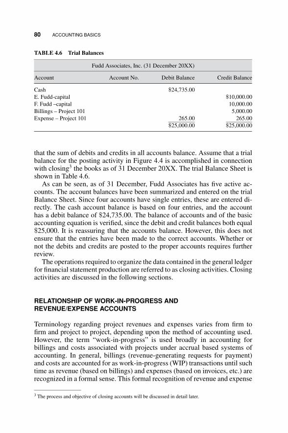
P1: OTA/XYZ P2: ABC



TABLE 4.6 Trial Balances

Fudd Associates, Inc. (31 December 20XX)

Account Account No. Debit Balance Credit Balance

Cash $24,735.00E. Fudd-capital $10,000.00F. Fudd –capital 10,000.00Billings – Project 101 5,000.00Expense – Project 101 265.00 265.00

$25,000.00 $25,000.00

that the sum of debits and credits in all accounts balance. Assume that a trialbalance for the posting activity in Figure 4.4 is accomplished in connectionwith closing3 the books as of 31 December 20XX. The trial Balance Sheet isshown in Table 4.6.

As can be seen, as of 31 December, Fudd Associates has five active ac-counts. The account balances have been summarized and entered on the trialBalance Sheet. Since four accounts have single entries, these are entered di-rectly. The cash account balance is based on four entries, and the accounthas a debit balance of $24,735.00. The balance of accounts and of the basicaccounting equation is verified, since the debit and credit balances both equal$25,000. It is reassuring that the accounts balance. However, this does notensure that the entries have been made to the correct accounts. Whether ornot the debits and credits are posted to the proper accounts requires furtherreview.

The operations required to organize the data contained in the general ledgerfor financial statement production are referred to as closing activities. Closingactivities are discussed in the following sections.

RELATIONSHIP OF WORK-IN-PROGRESS ANDREVENUE/EXPENSE ACCOUNTS

Terminology regarding project revenues and expenses varies from firm tofirm and project to project, depending upon the method of accounting used.However, the term “work-in-progress” is used broadly in accounting forbillings and costs associated with projects under accrual based systems ofaccounting. In general, billings (revenue-generating requests for payment)and costs are accounted for as work-in-progress (WIP) transactions until suchtime as revenue (based on billings) and expenses (based on invoices, etc.) arerecognized in a formal sense. This formal recognition of revenue and expense

3 The process and objective of closing accounts will be discussed in detail later.

P1: OTA/XYZ P2: ABC


RELATIONSHIP OF WORK-IN-PROGRESS AND REVENUE/EXPENSE ACCOUNTS 81

typically occurs at the point in time at which accounts are closed in order togenerate the Income Statement.

When income recognition occurs in the course of closing accounts, theWIP billings become revenue and the WIP costs become expenses. In thissense, the WIP accounts can be viewed as holding accounts in which revenueand expense information is gathered so that at closing the amount of revenueand expenses can be compared to calculate income. As you will see later, thiscalculation is the basis for recognizing income and calculating the associatedtaxes which must be paid. This progression of collecting billings and costinformation and, at closing, transforming it into revenue and expenses isshown schematically in Figure 4.5.

The terminology “work-in-progress” (as a prefix) may appear in a com-pany’s books as construction in progress (CIP), contracts in process, or somesimilar phrase. The general idea is, however, that both billings and costs are“in progress” until the moment at which they are declared revenues and ex-penses for purposes of income recognition. Therefore, at the time billingsand costs enter the bookkeeping system, they are typically carried in work-in-progress accounts until the point at which the closing of accounts occurs.This is a subtle point that has not been emphasized previously in discussingthe flow of project-related transactions. A better understanding can be gainedby studying transactions 2, 3, 6, and 8 in Appendix B.

One additional point deserves comment. At the time of closing accounts(i.e., the end of an accounting period—month, quarter, etc.), some revenueearned has not been billed to the client, and some expenses incurred maynot have been documented in terms of an invoice from the vendor or abilling from the appropriate subcontractor. Although these transactions have

Income(+ or –)

Journalizing

andposting

Point in time

of income recognition(closing of accounts or

completion of job)

*Invoices and payroll.

Billings

source

document

Cost*source

documents

WIP

billings

WIPcosts

Revenue

Expense

Figure 4.5 Concept of work-in-progress.

P1: OTA/XYZ P2: ABC



accrued, they have not been documented in terms of source documents. Sincethey have occurred, it is important include them in the financial statements.Payroll is a good example. Assume that closing to prepare financial reportsoccurs on the 15th of the month. If the office staff is paid monthly, halfof their pay will have accrued as an obligation by the 15th of the month.Similarly, half of a month’s rent will accrue on the company’s building andmust be reflected in any financial statement prepared as of the 15th of themonth.

The key idea is that, even though a transaction is not documented interms of a source document, if, in fact, a revenue or expense has accrued,this transaction should be accounted for at the time of closing accounts.Therefore, revenue earned but not billed should be recognized at closing.Expenses incurred at accrued for which invoices or billings have not beenreceived should also be recognized.

CLOSING THE ACCOUNTING CYCLE

At certain times, normally at the end of accounting periods, it is necessary tocheck on the financial health of the firm and its operations. Accounting periodsare determined on the basis of management needs and the requirementsof outside agencies for information concerning the financial status of thefirm. Accounting periods may be as short as one week or as long as onequarter. Government regulations impacting most firms require that reportsbe submitted for tax purposes on a quarterly basis. The so-called accountingcycle is terminated at the end of the accounting period by closing accountsand generating financial statements.

At the end of the accounting period, accounts are closed so as to recognizerevenue and expense flows that should be picked up in the Balance Sheet,Income Statement, and other relevant financial documents. The process ofclosing accounts causes revenues and expenses to be transferred from nominalaccounts to real accounts. Real accounts remain open from period to periodand their period end balances are reflected in the financial reports (e.g.,Balance Sheet, etc.). Nominal accounts are closed at the end of the accountingperiod by bringing their balances to zero. Revenue and expense accounts, suchas those associated with projects and other profit centers, are referred to asnominal accounts. At the end of the accounting period, the balances of theseaccounts are cleared out or transferred to real accounts, which link to reporteditems of summary information in the Balance Sheet and Income Statement.This process of clearing the nominal accounts brings the balance in theseaccounts to zero. The summarization of this clearing action appears in thereal accounts. Real account balances are reflected in the Income Statementand Balance Sheet. This act of closing nominal accounts results in incomerecognition (based on earned value).

P1: OTA/XYZ P2: ABC


RECOGNITION OF INCOME 83

RECOGNITION OF INCOME

The assessment of income earned on a construction project is complicatedsince the “sale” is, in effect, occurring across the life of the project. Thatis, the project itself is a large end item that will be paid for in incrementsthroughout the period of construction. If the project extends over severalaccounting periods, the question is “How much income should be recognizedin a given period?”

If the accrual basis of account is being used, it is possible to sumbillings to the client during a given period and view this as revenue forincome recognition purposes. However, on longer-term contracts use ofthe billings method can lead to deviation from the actual revenues earnedbase on work performed. That is, the amount billed may not be the amountearned.

The billings that are submitted by the construction contractor are calledprogress payment requests. These partial payments for a given period (usuallya month) of the total amount bid are calculated by estimating the amount ofwork performed in a given pay period. The client then pays the correspondingportion of the total work for the period just completed. Many factors (includ-ing the accuracy of the estimate of work completed) can cause a conditionreferred to as overbilling or underbilling. When revenue is based on progresspayments billed to a particular point in the project, the revenue (and associatedincome) billed may be either great than or less than the revenue earned. If thecumulative amount billed is greater than the revenue earned, an overbillinghas occurred. If the cumulative amount billed is less than the revenue earned,an underbilling condition exists.

Therefore, the billings method does not reflect the true financial position ofthe project (and the firm) because the income earned has been misrepresented.This problem develops on contracts that run over many progress paymentperiods. The problem of over and underbilling is typical of the long-term(multiperiod) construction projects.

Percentage-of-Completion Method of Income Recognition

In order to better reflect the actual revenue earned on a particular project ata given time, the percentage-of completion (POC) method can be used. Inthe POC method, gross revenue is recognized on each contract in proportionto the progress made on that contract. The revenue (and income) generatedbased on the progress is recognized whether or not it is billed to the client.The key criterion for recognizing revenue is that it has been earned. Thisgives a better indication of the firm’s position in the financial statement andis, therefore, the recommended method for income recognition and statementpreparation.

P1: OTA/XYZ P2: ABC



Several methods are used, in practice, to establish the percentage completedin terms of value earned at a particular point in the project’s life cycle. Theseare:

Cost-to-cost methodEffort-expended methodUnits-of-work-performed methods

The cost-to-cost or cost-completion method calculates the percentage com-plete on the basis of the following ratio:

Cost incurred to date on project/Estimated total cost of project

Another way of calculating this ratio is:

Cost incurred to date/Cost incurred to date + estimated cost to complete

In the effort-expended method, the percentage is based on the ratio ofunits of resource effort (e.g., man-hours or similar measure) to the total effortestimated to complete. This ratio can be expressed in terms of labor hours orlabor cost. Based on man-hours, the calculation could be made as follows:

Man-hours to date expended on project/Total estimated

man-hours on project

or, in terms of labor cost, as follows:

Labor cost incurred/Labor cost incurred + estimated labor cost to complete

This method of calculation tends to offset distortions in the cost-to-costmethod, which occur when materials are delivered to the site (and thereforecost is incurred) but are not installed (i.e., the revenue is not yet earned).

The problems inherent in both the cost-to-cost and effort-expended meth-ods relate to the fact that inefficient work during the early phases of the project(and the consequent higher expenses and/or resource expenditure) generatesapparently higher revenues by increasing the numerator of the ratios above.This tends to inflate the earned revenue amount.

To correct for inflated earned revenue, the percentage of completioncan be calculated by using physical units of production as the basis forcalculation. Using the units-of-work-performed method, we find that the POCratio becomes:

Units of work performed to date/Estimate total units of work in project

P1: OTA/XYZ P2: ABC


RECOGNITION OF INCOME 85

On a heavy construction earthwork job, this ratio might be:

Cubic yards of material excavated to date/Estimated total cubic

yards in project

This physical completion method of determining the POC is appropriateon projects where a single unit of work (e.g., cubic yard, lineal foot) can beidentified as representative of the work to be accomplished on the total project.It does, however, assume that revenue is generated and earned in proportionto the extent of physical completion of the selected work item. This methodneglects earned revenue associated with mobilization and demobilization ofthe job. For instance, if extensive haul and access roads must be constructedbefore the first lineal foot of pipeline can be constructed, using the footageof pipeline as the work unit would result in no revenues earned during theextended period of access road construction.

Clearly, all of the methods used to determine the percentage of completionare based on estimates. The American Institute of Certified Public Accoun-tants (AICPA) Construction Contractors: AICPA Audit and Accounting Guideindicates that the use of the percentage-of-completion method depends on theability to make reasonably dependable estimates.

In general, the POC method is the preferred method of income recognitionand should be used for all projects unless the unique and risk-associatedaspects of a particular project are so significant as to preclude developmentof reliable estimates.

Completed-Contract Method of Income Recognition

The basic idea underlying the completed-contract method is that the recog-nition of income is deferred until the end of the project. In general, for allprojects of any size and continuing over more than one quarter (e.g., threemonth period), use of this method is not allowed and, if used, is carefullyscrutinized by the federal and state tax agencies.

The advantage from the contractor’s point of view is that, at the endof the project, actual as-built information regarding the costs incurred andthe revenues generated is available. Therefore, a “settling up” can occur,which gives the most accurate evaluation of income generated by the project.The determination of project income is no longer dependent upon estimates.Income recognition and tax liability does not occur until the contract iscompleted.

In general, this deferment of tax payment is not viewed favorably byfederal and state tax agencies. In fact, this method has been misused to defertax payments over multiyear periods on billion dollar contracts. Litigation hasestablished that this use of the completed contract method is not appropriateand tax law has been modified to disallow the use of this method in such

P1: OTA/XYZ P2: ABC



cases. As a practical matter, the method can only be used by small contractors(e.g., small electrical and plumbing firms) who operate primarily on a workorder basis.

If the method is used for a project in progress during the generation of finan-cial reports, revenues and expenses are reported and maintained in “holdingaccounts” (e.g., Construction in progress – Job 103, etc.) until the projectis complete. In such cases, until the job is completed, progress paymentsreceived are considered as “advances” against the ultimate successful com-pletion of the work. These accumulated advances are shown as liabilitiesand are ultimately cleared as the end of the standard accounting period (e.g.,quarter).

The project expenses are considered to be contractor-owned assets untilthe project is accepted as complete by the owner. The accumulation of ex-penses is captured in appropriate accounts (e.g., Construction in progress –expenses – job 103). At completion, progress payments accumulated (i.e., allprogress payments received) are compared with the total cost accumulationto determine the income recognized.

TRANSACTIONS DURING A PERIOD

In order to understand the process of closing and statement preparation, itis necessary to consider the activity during an accounting period. During agiven period revenues and expenses occur randomly or on an “as scheduled”basis (e.g., submission of a progress payment request at the end of the month).These revenues and expenses are journalized and ultimately transferred to thegeneral ledger accounts. The Chart of Accounts (see Appendix A) being usedby a firm is a listing of all of the ledger accounts. In the following discussion,the general ledger accounts and the Chart of Accounts can be viewed assynonymous. As stated previously, the Chart of Accounts is organized intothe following:

Revenue accountsExpense accountsAsset accountsLiability accountsNet worth (or equity) accounts

In other words, the Chart of Accounts is organized so as to providefeeder information to the financial statements. By examining the accounts inAppendix A, it is possible to recognize this breakdown of accounts into thefive categories listed above. The movement of transactions to the generalledger accounts is shown in Figure 4.6.

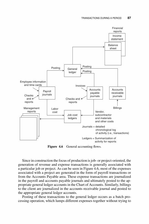
P1: OTA/XYZ P2: ABC


TRANSACTIONS DURING A PERIOD 87

Financial

reports

Income

statement

Balance

sheet

Posting

Posting

Invoices

Checks and

reports

Accounts

payablejournals

Accounts

receivablejournals

Billings

General

ledger

Posting

Employee information

and time cards

Payroll

journalsChecksand

reports

Management

reportsLabor

costJob costledgers

Vendor,subcontractor

and materialsand other costs

Journals = detailed chronological log

of activity (i.e., transactions)

Ledgers = Summarization of activity for reports

Figure 4.6 General accounting flows.

Since in construction the focus of production is job- or project-oriented, thegeneration of revenue and expense transactions is generally associated witha particular job or project. As can be seen in Figure 4.6, most of the expensesassociated with a project are generated in the form of payroll transactions orfrom the Accounts Payable area. These expense transactions are journalizedin the payroll and accounts payable journals and ultimately posted to the ap-propriate general ledger accounts in the Chart of Accounts. Similarly, billingsto the client are journalized in the accounts receivable journal and posted tothe appropriate general ledger accounts.

Posting of these transactions to the general ledger occurs as a batch pro-cessing operation, which lumps different expenses together without trying to

P1: OTA/XYZ P2: ABC



sort them for purposes of identification. That is, the weekly expenses of Job101 will be consolidated and batch posted to the single GL Work-in-progressaccount for a given project (i.e., Work-in-progress – expense – Job 101). Thisprocedure means that no attempt is made to relate the particular expense to aphysical or cost component.

Alternatively, a set of job cost accounts can be maintained to allocate coststo various cost centers (e.g., concrete—slab on grade, hand excavation, etc.).These job cost accounts can be thought of as Work-in-progress subsidiaryaccounts established to provide detailed cost reporting for each project. Thespecific purpose of these project accounts is to capture information linkingvarious costs to the detailed cost centers of the project with which they areassociated. Project cost accounts will be discussed in detail in Chapter 5. Atypical listing of project cost accounts is shown in Figure 5.4.

The simultaneous flow of information to the Chart of Accounts (GL ac-counts) and to the Job Cost accounts is shown schematically in Figure 4.6. Thecost accounts are established to obtain detailed information relating expensesto particular cost centers within the job.

POSTING TO THE GENERAL LEDGER DURINGTHE ACCOUNTING PERIOD

In order to understand the operation of the general ledger during a givenaccounting period, consider the situation presented in Figure 4.7.

It is assumed that Apex Construction has three projects in progress duringthe period under consideration. These three projects are numbered from 101to 103. The terminology used for Revenue- and Expense-related accounts isgiven in Table 4.7.

For purposes of demonstration, projects will use both the Percentage-of-Completion and Completed-Contract methods of income recognition. Thegeneral ledger account names used to record revenue and expense accumu-lation when using each method are given in Table 4.7. Projects 101 and 102will use the POC method. Project 103 will use the completed contract or CCmethod. This is summarized in Table 4.8.

As can be seen from Figure 4.7, billings associated with Projects 101and 102 are posted to revenue accounts within the Chart of Accounts (i.e.,billings -101 and billings-102). Similarly, expenses associated with these jobsare posted to the appropriate expense accounts (i.e., WIP – expense-101 andWIP-expense-102). The accumulation of these billings and expenses will beused at the end of the period to calculate the incremental amount of incometo be recognized.

The billings on the completed-contract job are not recognized at this timeas revenues. Recognition is deferred until the project is completed. Therefore,the billings for the CC project are posted to the appropriate advanced billings

P1: OTA/XYZ P2: ABC


POSTING TO THE GENERAL LEDGER DURING THE ACCOUNTING PERIOD 89

Job 101

REVENUE ACCOUNTS

Chart of Accounts

Billings – 101

Billings – 102

EXPENSE ACCOUNTS

Revenue – 103

WIP – Exp 101

WIP – Exp 102

Expense – G&A

All Const. in Progress

(CIP) Moved to Expenses

at end of Job

ASSET ACCOUNTS

CIP – 103

LIABILITY ACCOUNTS

Advanced Billings

AB – 103

Expense – 103

InProgress

AccountsReceivable

AccountsPayable

Job 102

In

Progress

Job 103

Completedthis

Period

A

A

A

A

B

B

B

B

G&AAccounts

Percentage of Completion

Jobs (101,102)

Completed Contract

Job (103)

Net Worth Accounts

AdvancedBillings Amount

is Transferred

to Revenue atEnd of Job

Figure 4.7 During-the-period transactions.

P1: OTA/XYZ P2: ABC



TABLE 4.7 General Ledger Accounts Posted When Using POC and CC

Method of income recognition

Type of transaction General Ledger under POC General Ledger under CC

Revenue Billings - Job X Advanced Billings - Job YCost Work-in-progress expense - Job X Construction in Progress - Job Y

account (i.e., AB 103). The costs and expenditures associated with this jobare not recognized at this time as expenses. They are, therefore, posted tothe appropriate construction-in-progress account (e.g., CIP-103), as shown inFigure 4.7.

The revenue postings when the POC method is used are balanced byappropriate entries to the asset account—Accounts Receivable. The AdvanceBillings postings when the CC method is used are also offset by balancingentries to Accounts Receivable, as shown by the arrow labeled A in Figure4.7. The expense posting under the POC method result in balancing entries tothe appropriate accounts payable ledge accounts (e.g., payroll, Jones Lumber,and the like). Similarly, the construction-in-progress amounts posted on theCC project are offset by entries to the appropriate accounts payable. Thesebalancing entries are shown by the arrows labeled B in Figure 4.7. TheAccounts Receivable and Accounts Payable themselves are general ledgeraccounts (that is, they are listed in the Chart of Accounts) and are shown inFigure 4.7 “pulled out” of their positions as asset and liability accounts forclarity of presentation.

The CC Project 103 is completed during the period under consideration.Since it is completed during this period, income will be recognized at the endof the period. When the project is completed, the accumulated expenses in theasset account “construction-in-progress – 103” are recognized as expensesand transferred to the account expense – 103.

Similarly, the accumulated billings in advanced billings -103 are recog-nized as revenues and transferred to the account Revenue 103. These actionsessentially consolidate entries and clear these “holding” accounts preparatory

TABLE 4.8 Example Summary Data

Method of Income EstimatedProject Recognition Amount Billed Bid Price Expense

101 POC $20,000 $100,000 $75,000102 POC $110,000 $200,000 $160,000103 CC Completed $250,000 $225,000

P1: OTA/XYZ P2: ABC


CLOSING ACTIONS AT THE END OF THE PERIOD 91

to income recognition at the end of the period. These flows are shown byarrows connecting the appropriate accounts in Figure 4.7.

General and Administrative costs are assumed to recognized on a period-by-period basis. Postings of these overhead-type costs are shown as entriesto the expense account G&A expenses.

CLOSING ACTIONS AT THE END OF THE PERIOD

At the end of the period, actions must be taken to “settle up” and recognizethe amount of income to be reported for the period. These are the closingactions that clear the revenue and expense accounts and lead to calculationsof income. In the case of Jobs 101 and 102, income is being recognizedperiod by period (i.e., on percentage-of-completion basis.) When recognizingincome with the Completed-Contract method, income is recognized only inthe period in which the job is completed. In this case, job 103 in completedin the period under consideration. Therefore, the profit achieved on the entireproject will be recognized in this period. Actions occurring at closing forthese three projects are shown schematically in Figure 4.8.

Income calculation for Projects 101 and 102 requires the calculation ofthe percentage complete. The cost-to-cost basis is used in this example. Theperiod expenses for Project 101 amounts to $25,000 versus the total esti-mated expense of $75,000. This means that the percentage complete is 33.3percent and the earned revenue is $33,333. The amount of income recognizedis (33,333 minus 25,000) $8,333. This is recognized in the account IncomeSummary and ultimately in the Income Statement. Comparing the amountbilled, $20,000 with the earned revenue, $33,333, indicates that an under-billing has occurred. This underbilling is posted to the asset account Costsand estimated earnings in excess of billings, and amounts to $13,333. Similaractions relating to Project 102 result in the recognition of $20,000 in income.The total estimated cost of $160,000 versus $80,000 expenses incurred indi-cates that the percentage complete is 50%. The earned revenue is $100,000and a profit of $20,000 is recognized in the Income Summary. On this project,an overbilling has occurred, since the amount billed ($110,000) is greater thanthe amount earned ($100,000). This overbilling of $10,000 is reflected in theliability account Billings in excess of costs and estimated earnings.

Project 103, which was completed during the period and on which thedeferred income will now be recognized is handled in a manner similar to thetwo percentage-of-completion contracts. The exception is that the expensesare compared to the total project bid price (i.e., the project is 100% complete).This is, of course, the advantage of the of Completed-Contract method. Weknow the expenses so the calculation of income recognized is not based on anestimate, but rather on final as-built amounts. Restrictions have been placedon the use of the CC method, however, and it can be used only in very specialsituations. As a practical matter, for projects that are completed over several

P1: OTA/XYZ P2: ABC


Reve

nu

e A

cco

un

tsP

rofit

= $

8,3

33

Pro

fit =

$2

0,0

00

Bill

ing

s –

10

1

Bill

ing

s –

10

2

Reve

nu

e –

10

3

Exp

en

se

Acco

un

ts

WIP

-Exp

en

se

10

1

WIP

-Exp

en

se

10

2

Exp

en

se

10

3

Pro

ject

Exp

en

se

Pro

ject

Reve

nve

Inco

me

Su

mm

ary

Un

de

r B

ill =

$1

3,3

33

Asse

ts

Costs

and E

stim

ate

dE

arn

ings in E

xcess

of

Bill

ings

Co

st in

Exc

ess

of

Bill

ing

s o

nU

nco

mp

lete

d C

on

tra

cts

Bill

ings in E

xcess

of C

osts

and E

st.

Earn

ings

Bill

ing

s in

Exc

ess

o

f C

ost

s o

n

Un

com

ple

ted

Co

ntr

act

s

Lia

bili

ties

Ove

r B

ill =

$1

0,0

00

Ne

t W

ort

h

Jo

b 1

01

Exp

en

se

= $

25

,00

0

Jo

b 1

02

Exp

en

se

= $

80

,00

0

Jo

b 1

01

Ea

rne

dIn

co

me

=

$3

3,3

33

Jo

b 1

02

Ea

rne

d

Inco

me

=$

10

0,0

00

Reve

nu

e 1

03

$2

50

,00

0

Jo

b 1

02

Bill

ing

s=

$1

10

,00

0

Jo

b 1

01

Bill

ing

s=

$2

0,0

00

Exp

en

se

10

3

$2

25

,00

0

A B

C

A

EB

D E C

D

< <<<

Ba

lan

ce

Sh

ee

t

Fig

ure

4.8

Clo

sing

actio

nsat

end

ofpe

riod

.

92

P1: OTA/XYZ P2: ABC



accounting periods the POC method is the method of income recognitionrequired by the Internal Revenue Service (IRS).

In this case, the bid price (modified by any change order amounts) iscompared to the actual expenses of $225,000. The earnings of $25,000 aretransferred at this time to the income summary. Earnings recognized onProjects 101,102, and 103 for this period amount to $53,333.


1. What is the difference between journalizing and posting?2. Is it possible to post into an asset account and a revenue account? Give

two examples with debiting and crediting an asset account.3. Today is 3 February 20XX. You are using the accrual method of account-

ing. You have received an invoice from Halco Industries in the amountof $565 for work performed on Project 101. You also mailed an invoiceto Ajax International for payment of work performed by your companyin the amount of $6,238 on Project 101. On 10 February you send acheck to Halco to cover their billing and receive a check from Ajax on12 February in the amount of your billing to them.Make the proper journal entries on a sheet captioned as in Table P4.1.

TABLE P4.1 Company Journal

Transaction# Date Description Debit Credit

4. Journalize the transactions shown in Table P4.2 for Tip Top Associates,Inc., incurred during the month of July 20XX (assume accrual basis).

TABLE P4.2 Transactions for Tip Top Associates

6-Jul Initializing capital deposited in bank $12,00010-Jul Office supplies purchased 25012-Jul Purchase computer 3,500

(paying $1000 with balance on account)15-Jul Office rent 42520-Jul Billing to Jones County Board of Education 1,25525-Jul Salaries—employee payroll 65528-Jul Paid on account for computer 80030-Jul Cost of expended supplies 145

P1: OTA/XYZ P2: ABC



5. Transactions during the period 1 December 2015 to 30 November 2016are given below for ABC Construction.

(1) Total income (fees) from construction contracts $400,000(2) Material inventory purchased on account 80,000(3) Total office rent paid 20,000(4) Salaries paid to engineers 90,000(5) Accounts receivable collected 60,000(6) Account payable paid 30,000(7) Subcontractor accounts paid 70,000(8) Bidding expenses 20,000(9) Building depreciation 40,000(10) Construction equipment depreciation 30,000

Using the transactions presented in Appendix B as a guide:� Journalize all of the above transactions.� Post journal entries to appropriate accounts.� Develop the Income Statement for period 1 December 2015 to 30

November 2016.� Develop the Balance Sheet for ABC Construction as of 30 November

2016.6. What is a “real” account? How does it differ from a nominal account?7. What is the reason for closing accounts?

TABLE P4.3 Balance Sheet, CPM Construction Company (31 December, 2013)

Assets Liabilities75,000 Accounts payable 85,000

Cash110,000 Notes payable 50,000

Accounts receivable300,000 Long-term loans 60,000

BuildingsLess accumulated depreciationon the buildings

(150,000) Total liabilities 195,000

240,000 Net worthConstruction equipment

Less accumulateddepreciation on equipment

(80,000) Capital stocks 250,000

20,000 Retained earnings 70,000Other assets

515,000 Total net worth 320,000Total assets

Total net worth and liabilities 515,000

P1: OTA/XYZ P2: ABC


REVIEW QUESTIONS AND EXERCISES 95TABLE P4.4 Transaction for CPM Construction Company

Transaction Date TransactionNumber

1 1/2/X4 CPM Co. bought construction equipment for $130,000 for whichthe company paid $15,000 cash and remaining on account.

2 2/4/X4 CPM Co. was billed $20,000 by Smith Material Supplier for costof material.

3 3/4/X4 CPM paid $20,000 to Smith Material Supplier related totransaction #2.

4 3/8/X4 CPM billed client for $320,000 (bill #1 on Job 101).5 4/7/X4 CPM was billed $60,000 by National Rental Co. for renting

construction equipment.6 5/8/X4 CPM received $290,000 from client for bill #1 on Job 101.7 6/7/X4 CPM paid $60,000 to the National Rental Co. for the bill received

on 4/7/X4.8 7/3/X4 CPM paid $70,000 cost of labor.9 8/16/X4 CPM was billed $45,000 by subcontractor.

10 9/16/X4 CPM paid $45,000 to the subcontractor for the bill received on8/16/X4.

11 10/1/X4 CPM billed client for $280,000 (bill #2 on Job 101).12 10/20/X4 Accounts receivable of $20,000 are collected.13 11/15/X4 CPM received $265,000 from client for bill #2.14 12/15/X4 Accounts payable of $40,000 are paid.15 12/25/X4 CPM paid $145,000 in payroll expense.16 12/30/X4 Dividends paid in the amount of $20,000 to stockholders.17 12/30/X4 Building depreciation of $30,000 recognized for the year.18 12/30/X4 CPM depreciates its construction equipment for the total of

$65,000 each year (this includes also the depreciation of theequipment bought on 1/2/X4.)

8. Can you think of construction contractors who can use the Completed-Contract method on a regular basis due to the type of contracts that theynormally undertake?

9. How are the Income Statement and Balance Sheet linked when closingaccounts?

10. The Balance Sheet of CPM Construction Company as of 31 December2013 is given in Table P4.3. Assume that this company is using the POCmethod of income recognition. Further, assume that 65% of the projectswith total bid price of $850,000 have been completed in 2014.(a) Journalize the following transactions. Identify each transaction as

asset, liability, revenue, expense, and so forth (Table P4.4).(b) Establish relevant accounts for posting. Divide them into categories

as Assets, Liabilities, and Net Worth.(c) Close accounts as of 31 December 2014.(d) Develop the Income Statement for the year 2014.(e) Develop the Balance Sheet as of 31 December 20X4.

P1: OTA/XYZ P2: ABC

JWBT106-05 JWBT106-Halpin June 26, 2009 15:46 Printer: Sheridan Books

CHAPTER 5

PROJECT-LEVEL COST CONTROL

OBJECTIVES OF PROJECT-LEVEL COSTCONTROL IN CONSTRUCTION

As had been emphasized in the first four chapters, construction is a project-based activity. In dealing with financial accounting, the focus has been on thecompany and the generation of revenue and income at the level of the firm.The company income is the aggregate of income generated from the projectsin progress (and completed) as well as other revenue-generating activities(e.g., equipment rental, etc.). We now must address the project level to betterunderstand how revenue and the associated income flows from these profitcenters are tied into the company-level accounting system.

Within the project format, there are a number of issues that are critical tomaking a given job profitable:

� Tracking costs to date is one of the primary jobs of a successful projectmanager.

� On more sophisticated projects, finding the earned value to date is essen-tial to avoiding cost overruns.

� Projection of profit to date, based on revenues and costs to date allowsthe PM to assess the profitability of the project.

� Actual costs must be compared to budgeted costs in order to determinewhether the project is on the cost profile originally predicted.

97



P1: OTA/XYZ P2: ABC


98 PROJECT-LEVEL COST CONTROL

� A viable cost control system must be developed to ensure the earlydetection and assessment of financial problems on the project.

� An effective cost control system must be able to detect and reflect bothprofitable and negative cost trends.

� A good cost control system can be the basis for accurate calculation ofunit costs, which can be used for pricing future work.

UNIQUE ASPECTS OF CONSTRUCTION COST CONTROL

Cost control in the manufacturing and service sectors is dealt with priorto the sale of the product or service. The manufacturer of a refrigerator orTV set knows the direct cost of manufacturing a given unit prior to sale. Inconstruction, the project is “sold” first, before the costs of construction areincurred. Since the cost is fixed on a manufactured item or service prior tosale, profit can be influenced by increasing or decreasing the sale price basedon the strength of the market.

In the manufacturing and service sectors, pricing may, and typically does,vary as units are sold over time. Both the retail and wholesale prices of alawn mower, for instance, vary over time based on market conditions. If themarket is strong and demand is high, the sales price of the product or servicecan be increased. In discussing the sale of bicycles in the Chapter 1, it wasnoted that if the initial sale price leads to low sales volume (customers are notattracted to purchase), the price can be reduced. Simply stated, if the marketis weak, the price of the unit of sale may be reduced. Conversely, a strongmarket usually supports an increase in price.

In construction, the price and revenue from the project are effectively fixedat the time the bid is quoted and accepted. Therefore, decisions, regardingpricing and profit are agreed to by the client and the contractor prior tobeginning construction.1 Since the price and levels of expected revenues are,as a practical matter, fixed when the bid is accepted, construction projectmanagers are primarily involved with management and control of costs. Thequoted price cannot be changed or renegotiated unless major deviation fromthe conditions, as shown in the contract documents, can be established.

Once the bid price is accepted by the client, project managers are focusedon cost control. The lower the cost, the greater the profit generated on a givenproject. Pricing is subject to very little variation. Therefore:

Project Profit = Bid Price as adjusted (Fixed) − Cost of Work (Variable)

1 Certain contracts (Unit price, Cost plus, etc.) do provide for small adjustments based on field conditionsand quantities installed.

P1: OTA/XYZ P2: ABC


TYPES OF COSTS 99

Because “cost of work” is the variable in this equation, managementis heavily involved in data collection, reporting, and analysis with the ob-jective of controlling and reducing (where possible) the project cost. Mostconstruction companies have developed cost control systems to capture vari-ations as they occur during construction.

TYPES OF COSTS

Contractor-incurred costs associated with the construction of a given facilityrelate to:

1. Direct cost consumed in the realization of a physical subelement of theproject (e.g., labor and material costs involved in pouring a footer).

2. Production support costs incurred by project-level support resources orrequired by the contract (e.g., the superintendent’s salary, site officecosts, builder’s risk insurance, etc.).

3. Costs associated with the operation and management of the company asa viable entity (i.e., General and Administrative “G & A” costs) suchas the costs associated with preparation of payroll in the home office,preparation of the estimate, marketing, and salaries of company officers.

The production support costs are normally referred as project indirect costsor field overhead. G & A costs are also referred to as home office overhead.All of these charges must be recovered before income to the firm is generated.

The term overhead is used loosely to refer to all non-direct costs (i.e., 2and 3 above) on the project. Overhead costs in construction are typically lessthan 5% of total project costs. Conversely, the direct cost percent of totalcost in construction is relatively high. By comparison, overheads in otherindustries tend be much higher than those in construction. For this reason,careful management of direct costs is critical to success in completing aconstruction project. (Why would overheads in the fast-food industry behigher than those in construction?)

THE CONSTRUCTION ESTIMATE

Project cost control starts with the estimate prepared to support submittalof a bid for any given project. In order to bid on a job, an estimate of alldirect, indirect, and home office overhead costs for the project is prepared.The line items and quantities required to complete the project are estimated(“taken off”) from its plans and specifications. The total cost associated witheach direct cost line item is the product of its quantity times its unit cost.Ideally, unit costs are based on data from past projects of a similar natureperformed by the company. In most cases, however, a project includes new

P1: OTA/XYZ P2: ABC



Figure 5.1 Typical estimate summary.

items whose unit cost must be obtained from published references or from adetailed analysis of each resource required by the item. A typical summaryestimate is shown in Figure 5.1.

The line items in the estimate can be referred to as estimating accounts.The costs developed during the estimating period form the basis of the projectbudget, which consists of cost accounts establishing target values and costgoals for the project.

When the estimate of costs is distributed across the life of the project byplotting cost amounts during each period of the project against time, the costestimate is transformed into a time-scaled budget. The budget also reflectscorrections and refinements made to the estimate following acceptance of the

P1: OTA/XYZ P2: ABC


COST CONTROL SYSTEM 101

bid and prior to commencement of the work. There is normally a one-to-onerelationship between the estimating accounts in the estimate and the costaccounts in the project budget. The costs developed during the estimatingphase are transferred to the budget and represent target values against whichfield costs and performance can be measured.

COST CONTROL SYSTEM

In construction, each project is unique and requires a customized cost con-trol system. The project cost control system is a management informationsystem that gathers cost data designed to aid the manager in controlling theproject. As such, the project cost control system is to the manager what thecockpit dials and instruments are to the pilot of an airplane. It is a monitoringsystem designed to provide timely feedback to management regarding actualperformance on a given project vis-a-vis project performance goals, such asthose contained in the project budget. A secondary function of the job costsystem is the collection of data to be used as a basis for estimating future jobs.The system collects historical data on actual costs of labor, equipment, andmaterials, which provide reference information in pricing out future projects.Therefore, the cost control system serves two major functions: (1) cost mon-itoring and control versus the project budget, and (2) collection of data forestimating future projects.

As construction proceeds, field data are collected in the appropriate jobcost accounts. At this point, the project manager is in a position to compareactual field data with the expectations reflected in the budget. Variancesare monitored between expected costs and actual field production rates andcharges. By examining the variances, the manager can detect which accountsare seriously deviating from planned progress and can take corrective action.This approach is often referred to as management by exception. A conceptualdiagram of the relationship of the financial accounting and cost accountingsystems is shown in Figure 5.2. Cost management focuses on monitoring andcontrolling the cash flowing into and through the project cost accounts.

BUILDING A COST CONTROL SYSTEM

The form and design a of a cost control system depends upon the needs of thecontractor and the effort that must be expended to implement and maintainthe system. As with all management systems, the effort and time expendedin operating the system must be weighed against the savings achieved byusing the system. To be effective, the cost control system must produce theright amount of information at the right time (e.g., think pilot and aircraftinstruments). The extent to which project management supports a project

P1: OTA/XYZ P2: ABC



Balance sheet

Liabilities

Assets

Networth

Net =

Expenses

Revenue

Income statement

Financialaccounting

system

Billings

Estimates

Estimate

converted tobudgets

Estimate

Estimatingaccounts

(line items)

Estimatingdata base

Computer

Field costdata retained

for future

estimates

Estimatingaccount values

are transferredto cost accounting

system to becompared with

field data

Projectexpense (cost)

accounts

Variances betweenbudget and field

report areexamined - triggerscorrective actions

Costdatafromfieldreports

Time cards

Quantity

Job site

Figure 5.2 Cost control system layout.

control system depends upon management attitude, the financial risks inherentin the form of contract and the size of the profit margin.

The design, implementation, and maintenance of a project cost control sys-tem can be considered a multistep process. The five steps shown schematicallyin Figure 5.3 form the basis for establishing and maintaining a cost controlsystem. The following questions regarding each step in the implementationof the cost control system must be addressed:

1. Chart of cost accounts. What will be the basis adopted for developingestimated project expenditures, and how will this basis be related tothe firm’s general accounts and accounting functions? What will be thelevel of detail adopted in defining the project cost accounts, and howwill they interface with the general ledger accounts of the company’sfinancial accounting system?

2. Project cost plan/budget. How will the cost accounts be utilized to allowcomparisons between the project estimate and budget with actual costsas recorded in the field? How will the project budget estimate be relatedto the construction plan and schedule in the formation of a project costcontrol framework?

3. Cost data collection. How will cost data be collected and integrated intothe cost-reporting system?

P1: OTA/XYZ P2: ABC


COST ACCOUNTS 103

Step 1 Chart of cost accounts

Step 2 Project cost plan

Step 3 Cost data collection

Step 4 Project cost reporting

Step 5 Cost engineering

1Chart of

costaccounts

2Project

costplan

Costengineering

decisionmaking

5

Datareporting

Database forfuture

estimates

Datacollection

Projectstatus

Projectenvironment

43

Projectplans anddocuments

Figure 5.3 Steps in cost control.

4. Project cost reporting. What project cost reports are relevant and re-quired by project management in its cost management of the project?

5. Cost engineering. What cost engineering procedures should projectmanagement implement in its efforts to minimize costs?

These are basic questions that management must address in setting up thecost control system.

COST ACCOUNTS

Cost accounts define the level of detail at which job cost information will bemaintained. Cost accounts can be very rudimentary or very detailed, depend-ing on the complexity of the project and the needs of management. Cousin

P1: OTA/XYZ P2: ABC



Elmer and Uncle Fudd of Fudd Associates may decide to define just four costaccounts for each project as follows:

1. Labor Cost2. Equipment Cost3. Material Cost4. Other Costs

This amounts to keeping four physical folders into which documents foreach of the four types of costs are aggregated. This level of detail is, of course,very coarse and is not particularly helpful in locating potential cost overrunsor for estimating future jobs.

The more complex the project, the finer the level of detail must be. Thenumerical or alphanumeric designations of individual line items defined forcontrol purposes are called cost codes. Therefore, cost accounts are definedin terms of a cost code or numbering system.

The cost accounts can be thought of as a subsection of the overall chart ofaccounts (which includes revenue and other general ledger accounts). Projectcost accounts link to the Project expense accounts in the general ledger (G/L).Depending upon the desires of management and the purpose of the projectcost control system, these accounts can be fully integrated into the generalledger.

Many contractors find it desirable to maintain the cost accounts separatelyfrom the G/L accounts. The aggregate amounts of the individual cost accountsare posted to summary (work in progress) expense accounts for each project.This approach is shown conceptually in Transaction 3 of Appendix B.

COST ACCOUNT STRUCTURE

The first step in establishing a project cost control system is the definition ofproject-level cost centers. The primary function of the cost account breakdownis to divide the total project into significant units of work that can be measuredin the field (see Figure 5.4).

In most construction firms, cost systems have a structured sequence cor-responding to the order of appearance of the various trades or types of con-struction processes typical of the company’s construction activity. Heavyconstruction contractors are interested in earthwork-related accounts such asgrading, ditching, clearing and grubbing, and machine excavation. Referencesand information published by the American Road and Transportation BuildersAssociation (ARTBA) emphasize these type of accounts. The MasterFormatpublished by the Construction Specifications Institute focuses on buildingor vertical construction accounts. A breakdown of the major classifications

P1: OTA/XYZ P2: ABC


COST ACCOUNT STRUCTURE 105

MASTER LIST OF PROJECT COST ACCOUNTSSubaccounts of General Ledger Account 80.000

PROJECT EXPENSEProject Work Accounts Project Overhead Accounts100–699 700–999

100 Clearing and grubbing 700 Project administration101 Demolition .01 Project manager102 Underpinning .02 Office engineer103 Earth excavation 701 Construction supervision104 Rock excavation .01 Superintendent105 Backfill .02 Carpenter foreman115 Wood structural piles .03 Concrete foreman116 Steel structural piles 702 Project office117 Concrete structural piles .01 Move in and move out121 Steel sheet piling .02 Furniture240 Concrete, poured .03 Supplies

.01 Footings 703 Timekeeping and

.05 Grade beams .01 security

.07 Slab on grade .02 Timekeeper

.08 Beams .03 Watchmen

.10 Slab on forms 705 Guards

.11 Columns .01 Utilities and services

.12 Walls .02 Water

.16 Stairs .03 Gas

.20 Expansion joint .04 Electricity

.40 Screeds 710 Telephone

.50 Float finish 711 Storage facilities

.51 Trowel finish 712 Temporary fences

.60 Rubbing 715 Temporary bulkheads

.90 Curing 717 Storage area renta!245 Precast concrete 720 Job sign260 Concrete forms 721 Drinking water

.01 Footings 722 Sanitary facilities

.05 Grade beams 725 First-aid facilities

.07 Slab on grade 726 Temporary lighting

.08 Beams 730 Temporary stairs

.10 Slab 740 Load tests

.11 Columns 750 Small tools

.12 Walls 755 Permits and fees270 Reinforcing steel 756 Concrete tests

.01 Footings 760 Compaction tests

.12 Walls 761 Photographs280 Structural steel 765 Surveys350 Masonry 770 Cutting and patching

.01 8-in. block 780 Winter operation

.02 12-in. block 785 Drayage

.06 Common brick 790 Parking

.20 Face brick Protection of adjoining property

.60 Glazed tile 795 Drawings400 Carpentry 796 Engineering440 Millwork 800 Worker transportation500 Miscellaneous metals 805 Worker housing

.01 Metal door frames 810 Worker feeding

.20 Window sash 880 Genera! clean-up

.50 Toilet partitions 950 Equipment560 Finish hardware .01 Move in620 Paving .02 Set up680 Allowances .03 Dismantling685 Fencing .04 Move out

Figure 5.4 List of typical project expense (cost) accounts.

P1: OTA/XYZ P2: ABC



within the MasterFormat account system is shown in Table 5.1. A por-tion of the second level of detail for the classifications 0 to 3 is shown inFigure 5.5.

PROJECT COST CODE STRUCTURE

Once project cost accounts are established, each account is then assignedan identifying numeric or alphanumeric code known as a cost code. Oncesegregated by associated cost centers, all the elements of expense constitutinga work unit can be properly recorded by cost code.

A variety of cost-coding systems exists in practice, and standard chartsof account are published by organizations such as the National Associationof Home Builders (NAHB), Associated General Contractors (AGC), and theConstruction Specifications Institute (CSI) These standardized codes are veryuseful when a contractor needs to use manuals or other types of publishedinformation to estimate a unit of price for a line item. Standardization allowsa uniform definition of the item, its unit of measure, and even its location inthe estimate. Furthermore, sections in project specifications usually followthe structure of a standard code, thus simplifying the cross-referencing ofitems in the project’s cost estimate and its drawings.

The MasterFormat code as used in the R.S. Means Building ConstructionCost Data identifies three levels of detail. At the highest level, the majorwork classification, as given in Table 5.1, is defined. Also at this level, majorsubdivisions within the work category are established. For instance, 030-levelaccounts pertain to concrete, while 031 accounts are accounts specificallydealing with concrete forming. In a similar manner, 032 accounts are reservedfor cost activity associated with concrete reinforcement.

At the next level down, a designation of the physical component or subele-ment of the construction is established. This is done by adding three digitsto the work classification two-digit code. For instance, the three-digit codefor footings is 158. Therefore, the code 031158 indicates an account dealingwith concrete forming costs for footings.

At the third and lowest level, digits specifying a more precise definitionof the physical subelement are used. For instance an account code of 031158 5000 can indicate that this account records costs for forming concretefootings of a particular type (see Figure 5.6). This level of refinement isvery great, and the account can be made very sensitive to the peculiaritiesof the construction technology to be used. Further refinement could differ-entiate between forming different types of footings with different types ofmaterial.

At this level, the cost engineer and construction manager have a greatdeal of flexibility in reflecting unique aspects of the placement technologythat lead to cost fluctuations and thus must be considered in defining costcenters.

P1: OTA/XYZ P2: ABC


PROJECT COST CODE STRUCTURE 107

TABLE 5.1 Major Divisions in CSI’s MasterFormat UniformConstruction Index 2004

Procurement ands Contracting subgroup00 – Procurement and Contracting Requirements

General Requirements subgroup01 – General Requirements

Facilities Construction subgroup02 – Existing Conditions03 – Concrete04 – Masonry05 – Metals06 – Wood, Plastics, and Composites07 – Thermal and Moisture Protection08 – Openings09 – Finishes10 – Specialties11 – Equipment12 – Furnishings13 – Special Construction14 – Conveying Equipment15 – Reserved for future use in Mechanical16 – Reserved for future use in Electrical

Facilities Services subgroup21 – Fire Suppression22 – Plumbing23 – Heating Ventilating and Air Conditioning25 – Integrated Automation26 – Electrical27 – Communications28 – Electronic Safety and Security

Site and Infrastructure subgroup31 – Earthwork32 – Exterior Improvements33 – Utilities34 – Transportation35 – Waterway and Marine Construction

Process Equipment subgroup40 – Process Integration41 – Material Processing and Handling Equipment42 – Process Heating, Cooling, and Drying Equipment43 – Process Gas and Liquid Handling, Purification and Storage Equipment44 – Pollution Control Equipment45 – Industry-Specific Manufacturing Equipment48 – Electrical Power Generation

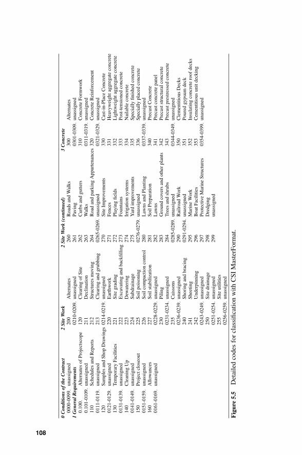
P1: OTA/XYZ P2: ABC


0C

ondi

tions

ofth

eC

ontr

act

2Si

teW

ork

2Si

teW

ork

(con

tinue

d)3

Con

cret

e00

00-0

099.

unas

sign

ed20

0A

ltern

ates

260

Roa

dsan

dW

alks

300

Alte

rnat

es1

Gen

eral

Req

uire

men

ts02

10-0

209.

unas

sign

ed26

1Pa

ving

0301

-030

9.un

assi

gned

0.10

0.A

ltern

ates

ofPr

ojec

tsco

pe12

0C

lear

ing

ofSi

te26

2C

urbs

and

gutte

rs31

0C

oncr

ete

Form

wor

k0.

101-

0109

.un

assi

gned

211

Dec

linat

ion

263

Wal

ks03

11-0

319.

unas

sign

ed11

0Sc

hedu

les

and

Rep

orts

212

Stru

ctur

esm

ovin

g26

4R

oad

and

park

ing

App

urte

nanc

es32

0C

oncr

ete

Rei

nfor

cem

ent

0111

-011

9.un

assi

gned

213

Cle

arin

gan

dgr

ubbi

ng02

65-0

269.

unas

sign

ed03

21-0

329.

unas

sign

ed12

0Sa

mpl

esan

dSh

opD

raw

ings

0214

-021

9.un

assi

gned

270

Site

Impr

ovem

ents

330

Cas

t-in

-Pla

ceC

oncr

ete

0121

-012

9.un

assi

gned

220

Ear

thw

ork

271

Fenc

es33

1H

eavy

wei

ghta

ggre

gate

conc

rete

130

Tem

pora

ryFa

cilit

ies

221

Site

grad

ing

272

Play

ing

field

s33

2L

ight

wei

ghta

ggre

gate

conc

rete

0131

-013

9.un

assi

gned

222

Exc

avat

ing

and

back

fillin

g27

3Fo

unta

ins

333

Post

-ten

sion

edco

ncre

te14

0C

lean

ing

Up

223

Dew

ater

ing

274

Irri

gatio

nsy

stem

s33

4N

aila

ble

conc

rete

0141

-014

9.un

assi

gned

224

Subd

rain

age

275

Yar

dim

prov

emen

ts33

5Sp

ecia

llyfin

ishe

dco

ncre

te15

0Pr

ojec

tclo

seou

t22

5So

ilpo

ison

ing

0276

-027

9.un

assi

gned

336

Spec

ially

plac

edco

ncre

te01

51-0

159.

unas

sign

ed22

6So

ilco

mpa

ctio

nco

ntro

l28

0L

awns

and

Plan

ting

0337

-033

9.un

assi

gned

160

Allo

wan

ces

227

Soil

stab

iliza

tion

281

Soil

Prep

arat

ion

340

Prec

astC

oncr

ete

0161

-016

9.un

assi

gned

0228

-022

9.un

assi

gned

282

Law

ns34

1Pr

ecas

tcon

cret

epa

nel

230

Pilin

g28

3G

roun

dco

vers

and

othe

rpl

ants

342

Prec

asts

truc

tura

lcon

cret

e02

31-0

234.

unas

sign

ed28

4T

rees

and

shru

bs34

3Pr

ecas

tpre

stre

ssed

conc

rete

235

Cai

sson

s02

85-0

289.

unas

sign

ed03

44-0

349.

unas

sign

ed02

36-0

239.

unas

sign

ed29

0R

ailr

oad

Wor

k35

0C

lem

entit

ious

Dec

ks24

0Sh

orin

gan

dbr

acin

g02

91-0

294.

unas

sign

ed35

1Po

ured

gyps

umde

ck24

1Sh

eetin

g29

5M

arin

eW

ork

352

Insu

latin

gco

ncre

tero

ofde

cks

242

Und

erpi

nnin

g29

6B

oatF

acili

ties

353

Cem

entit

ious

unit

deck

ing

0243

-024

9.un

assi

gned

297

Prot

ectiv

eM

arin

eSt

ruct

ures

0354

-039

9.un

assi

gned

250

Site

drai

nage

298

Dre

dgin

g02

51-0

254.

unas

sign

ed29

9un

assi

gned

255

Site

utili

ties

0256

-025

9.un

assi

gned

Fig

ure

5.5

Det

aile

dco

des

for

clas

sific

atio

nw

ithC

SIM

aste

rFor

mat

.

108

P1: OTA/XYZ P2: ABC


PROJECT COST CODE STRUCTURE 109

MasterFormat Mediumscope

MasterFormat Division

031 CREW DAILYOUTPUT

LABOR-HOURS UNIT

MAT.

305 .105 SFCA 1.51 2.50 .09 4.10 5.75

LABOR1996 BARE COSTS

158

5000 Spread footings, 1 use

FORMS IN PLACE, FOOTINGS Continuous wall, 1 use C-1

EQUIP. TOTALTOTAL

INCL. O&PStruct C.I.P. Formwork

031

031 Concrete Formwork

031100158 5000

Means Subdivision

Means Major ClassificationMeans Individual Line Number

Figure 5.6 Cost (line item) structure in the MasterFormat code.

Large and complex projects in industrial and energy-related constructionmay require cost codes that reflect additional information, such as the projectdesignation, the year in which the project was started, and the type of project.Long and complex codes in excess of 10 digits can result. An example of sucha code is shown in Figure 5.7. This code, consisting of 13 digits, specificallydefines the following items:

1. Year in which project was started (2014).2. Project control number (15).3. Project type (5 for power station).4. Area code (16 for boiler house).5. Functional division (2, indicating foundation area).6. General work classification (0210, indicating site clearing).7. Distribution code (6, indicating construction equipment).

Project classification

1 4 1 5 5 – 1 6 2 – 0 2 1 0 – 6

6

Specific

classification

Construction

equipment

General work classification

0210 – Site clearing

Functional division within project

Boiler house

foundation area

16

2

Project initiation year

Project number

Project type 5 = power

Figure 5.7 Classification of accounts: Typical data structure.

P1: OTA/XYZ P2: ABC



The distribution code establishes what type of resource is being costed tothe work process (i.e., clearing), the physical subelement (i.e., foundations) inwhat area of which project. Typical distribution codes might be as follows:

1. Labor2. Permanent materials3. Temporary materials4. Installed equipment5. Expendables6. Construction equipment7. Supply8. Subcontract9. Indirect

Clearly, these codes “slice and dice” the project into a very high level ofdetail. This makes the four cost folders used by Fudd Associates, Inc. lookpretty paltry. An impressive concentration of information can be achieved byproper design of the cost code. Such codes are also ideally suited for dataretrieval, sorting, and assembly of reports on the basis of selected parameters(e.g., all construction equipment costs for concrete forming on project 10started in a given year). The desire to cram too much information into costcodes, however, can make them so large and unwieldy that they are confusingto upper-level management.

COST ACCOUNTS FOR INTEGRATED PROJECT MANAGEMENT

In large and complex projects, it is advantageous to break the project intocommon building blocks for control both of cost and time. The concept ofa common unit within the project that integrates both scheduling and costcontrol has led to the development of the work breakdown approach. Thebasic common denominator in this scheme is the work package, which is asubelement of the project on which both the cost and time data are collectedfor project status reporting. The collection of time and cost data based on workpackages has led to the term integrated project management. That is, the statusreporting function has been integrated at the level of the work package. Theset of work packages in a project constitutes its work breakdown structure(WBS).

The work breakdown structure and work packages for control of aproject can be defined by developing a matrix similar to the one shown inFigure 5.8. The columns of this matrix are defined by breaking the projectinto physical subcomponents. Thus, we have a hierarchy of levels that beginswith the project as a whole and, at the lowest level, subdivides the project into

P1: OTA/XYZ P2: ABC


Pro

ject bre

akdow

n

str

uctu

re

Pro

ject

Syste

m A

Fo

un

da

tio

ns

Foundation 1

Foundation 2

Etc.

Etc.

Etc.

Etc.

Fans

Pumps

Area 1

Area 1

Area 2

Area 2

Ele

ctr

icity

Pip

ing

Me

ch

an

ica

l

Oth

er

syste

m/s

tructu

re

Responsib

ility

/task

bre

akdow

n s

tructu

re

Eart

hw

ork

tasks

Concre

teta

sks

Fra

min

gta

sks

Wire

pulli

ng

Term

inations

Work

packages

for

contr

ol

Etc

.

Pip

e fitting

tasks

Pip

e e

rection

tasks

Etc

.

Subcontr

acto

r A

Subcontr

acto

r BE

tc.

Project manager

General superintendent

Civil

superintendent

Electrical

superintendent

Piping

superintendent

Fig

ure

5.8

Proj

ectc

ontr

olm

atri

x.

111

P1: OTA/XYZ P2: ABC



General expense resources

Small tools

Construction equipment

Construction materials

Permanent materials

Craft labor

Project breakdown

DF441 Place & vibrate

concrete in foundationsdirect chute

121002 Boiler building foundation

(None this work package)

(None this work package)(None this work package)

6000 Smalls tools5104 Vibrators

2121 Concrete1110 Laborers

1190 Cement workers

Task/r

esponsib

ility

bre

akdow

n

Resourc

es

Work packages

Figure 5.9 Three-dimensional visualization of work-package-oriented cost ac-counts.

physical end items such as foundations and areas. As shown in Figure 5.8, theproject is subdivided into systems. The individual systems are further dividedinto disciplines (e.g., civil, mechanical, electrical). The lowest level of thehierarchy indicates physical end items (foundation 1, etc.). Work packages atthis lowest level of the hierarchy are called control accounts.

The rows of the matrix are defined by technology and responsibility. Atthe lowest level of this hierarchy, the responsibilities are shown in terms oftasks, such as concrete, framing, and earthwork. These tasks imply variouscraft specialties and technologies. Typical work packages then are defined,for example, as concrete tasks on foundation 1 and earthwork on foundations1 and 2.

This approach can be expanded to a three-dimensional matrix by consider-ing the resources to be used on each work package (see Figure 5.9). Using thisthree-dimensional breakdown, we can develop definition in terms of phys-ical subelement, task, and responsibility, as well as resource commitment.A cost code structure to reflect this matrix structure is given in Figure 5.10This 15-digit code defines units for collecting information in terms of workpackage and resource type. Resource usage in terms of monetary units, quan-tities, man-hours, and equipment-hours for a foundation in the boiler building

P1: OTA/XYZ P2: ABC


EARNED VALUE ANALYSIS 113

Project breakdown (length andformat varies with projects)

Task/responsibility code1st alpha–direct (D) or indirect (I)

2nd alpha–major category of work3rd–5th digits–detail

Resources1st digit–major accounting category

2–4th digits–detail

(As required for a

given work package)Work package

N N N N N N – A A N N N N N N N

N N N NN N N N

Figure 5.10 Basic cost code structure.

would be collected under work package code 121002. If this work relatesto placement and vibration of concrete by using a direct chute, the code isexpanded to include the alphanumeric code DF441. The resource code forthe concrete is 2121. Therefore, the complete code for concrete in the boilerbuilding foundations placed by using a chute would be 121002-DF441-2121.

This code allows collection of cost data at a very fine level. Schedul-ing of this work is also referenced to the work package code as shown inFigure 5.11. The schedule activities are shown in this figure as subtasksrelated to the work package.

EARNED VALUE ANALYSIS

Earned Value Analysis (EVA), also known as Earned Value Management(EVM), is the main formal project cost control technique currently used inconstruction. It also integrates elements of schedule control, using simplemeasures that can be understood by most construction professionals.

To illustrate the context for EVA, consider a situation where a carpetinstalling subcontractor has agreed to complete a contract for a six-storybuilding. The owner will furnish all materials and pay the subcontractor bytime billed. The contract specifies a duration of three weeks at a cost of$450,000. Two weeks into the job, two stories have been carpeted, but fourstories remain untouched. Furthermore, the carpet installed so far has costhalf of the total budget for this item. Most people will conclude that it is verylikely that this subcontractor will take longer than planned to complete itscontract and will end up with a cost overrun. If finishing two floors out of sixhas taken two weeks, isn’t it reasonable to infer that the total job will take sixweeks? Or that the total cost will be 150% of the budget, since one third of

P1: OTA/XYZ P2: ABC


Pro

ject bre

akdow

n

str

uctu

re

Pro

ject

Syste

m A

Fo

un

da

tio

ns

Foundation 1

Foundation 2

Etc.

Etc.

Etc.

Etc.

Fans

Pumps

Area 1

Area 2

Area 2

Ele

ctr

icity

Pip

ing

Me

ch

an

ica

l

Oth

er

syste

m/s

tructu

re

Responsib

ility

/task

bre

akdow

n s

tructu

re

Eart

hw

ork

tasks

Concre

teta

sks

Fra

min

gta

sks

Wire

pulli

ng

Term

inations

Subta

sks

(work

packages)

Etc

.

Pip

e fitting

tasks

Pip

e e

rection

tasks

Etc

.

Subcontr

acto

r A

Subcontr

acto

r BE

tc.

Project manager

General superintendent

Civil

superintendent

Electrical

superintendent

Piping

superintendent

Fig

ure

5.11

Proj

ectc

ontr

olm

atri

xw

ithsc

hedu

ling

ofsu

btas

ks.

114

P1: OTA/XYZ P2: ABC



the work has taken half of the budget? These figures are simple extrapolationsof the performance so far, and reflect the assumption that the cost and timeperformance rates up to now are representative of the rates for the remainderof this subcontractor’s job.

EVA uses exactly the preceding thought process to assess whether a projectis ahead or behind schedule, and whether it will cost less or more than itsbudget. It compares the value of the work performed to date (its “earned”value) with the value of the work planned to have been done to date andwith the actual cost of the work to date. If the earned value is less than theplanned value, EVA will report that the project is behind schedule. If theearned value is less than the actual cost, it will report that the project is overbudget.

EVA’s rationale for tracking cost and schedule is as simple as it is power-ful. Its validity is confirmed by its use throughout many years and in manyprojects. It was originally implemented by the Department of Defense in thelate 1970s to help better control complex projects. This original system wascalled the Cost and Schedule Control Systems Criteria or C/SCSC. It provedto be so effective that other government agencies (e.g., Department of En-ergy, etc.) adopted C/SCSC as a means of maintaining oversight on complexprojects such as nuclear and conventional power plants. Private owners suchas power companies implemented similar systems, since reporting to variousgovernment authorities encouraged or required the use of C/SCSC and earnedvalue concepts. Nowadays, EVA is supported by virtually all scheduling andcost control packages such as Primavera Project Planner R© and MicrosoftProject R©. Its principles permeate the management of virtually all large con-struction projects, even in cases where their project managers may not beexplicitly aware of the technique as discussed in this section.

The idea of earned value is based upon a rigorous development of percentcomplete of the budgeted costs associated with individual work packages orline items. Each work package has an initial budget or estimate which isdefined as the Budgeted Cost at Completion or BCAC. As work proceeds onan individual work package or account, assessment of the percent complete ismade at various study dates. The initial schedule establishes an expected levelof work completion as of the study date. The level of expected productionis often shown as an S-curve plotting the cost or units of production (e.g.,units produced, work hours expended, etc.) against time. This cost/productioncurve is referred to as the baseline. At any given time (study date), the unitsof cost/production indicated by the baseline are called the Budgeted Cost ofWork Scheduled (BCWS).

The tracking system requires that field reports provide information aboutthe Actual Cost of Work Performed (ACWP) and the Actual Quantity ofWork Performed (AQWP). The “earned value” is the Budgeted Cost of WorkPerformed (BCWP). The relative values for a given work package or accountat a given point in time (see Figure 5.12) provide information about the status

P1: OTA/XYZ P2: ABC



Cost/Prod. Units

Baseline

BCAC

TimeStudy Date

BCWS

ScheduleVariance Cost

Variance

ACWP

BCWP

Figure 5.12 Control values for Earned Value Analysis.

in terms of cost and schedule variance. The six parameters that form thefoundation of the “earned value” concept are:

1. BCWS. Budgeted Cost of Work Scheduled = Value of the baseline ata given time ACWP: Actual Cost of Work Performed; Measured in thefield.

2. ACWP. Actual Cost of Work Performed – Measured in the field.3. BCWP. Budgeted Cost of Work Performed = [% Complete] × BCAC.4. BCAC. Budgeted Cost At Completion = Contracted Total Cost for the

Work Package.5. AQWP. Acutal Quantity of Work Performed – Measured in the field.6. BQAC. Budgeted Quantity at Completion – Value of the Quantity Base-

line as Projected at a Given Point.

In order to put these terms into context, consider the small project shownin Figure 5.13 The project consists of two control accounts: A and B. “A”consists of two subaccounts, A.1 and A.2. The study date (e.g., September 1,etc.) information for these work packages is given in TABLE 5.2. In thisexample, the budget is expressed in worker hours so the baseline for controlis in worker hours. The estimated total number of worker hours for this scope

P1: OTA/XYZ P2: ABC



PROJECT

A

A. 1 A. 2

B

Figure 5.13 A simple project hierarchy.

of work is 215 (the sum of the estimated worker hours for A.1, A.2, and B).The BCWP, or earned value for a given work package, is given as:

BCWPi = PCi × BCACi

Where i is the work package or account label, and PC is the percent completeas of the study date.

The percent complete (PC) for each package is based on the ratio of theActual Quantities (AQWP) divided by the Budgeted Quantity at Completion(BQAC) based on the latest quantity assessment. If we know that the originalquantity estimate is 100 units, but updated information indicates that a totalof 120 units will be required to complete the work, completion of 50 unitswould not indicate 50 percent complete. The correct PC would be 50/120(e.g., AQWP/BQAC).

Based on the information in Table 5.2, the PC for each work package inthe small project would be:

PC(A.1) 35/105 = 0.333

PC(A.2) 60/77 0.780

PC(B) = 100/125 0.800

TABLE 5.2 Study Date Data for Simple Project

BCAC ACWP BQAC AQWP PC (%) BCWP ECAC

AA.1 100 40 105 35 33.3 33.3 120A.2 50 35 77 60 78.0 39.0 45B 65 50 125 100 80.0 52.0 62.5Total 215 125 — — 57.8 124.3 227.5

Project PC (PPC) = Total BCWP = 124.3 ÷ 215 = 57.8%ECACi = Estimated Cost at Completion for Work Package i = ACWPi/PCi

P1: OTA/XYZ P2: ABC



Then

BCWP (Project) = .333 (100) + .78 (50) + .8 (65)

= 33.3 + 39 + 52 = 124.3

Therefore, the Project Percent Complete (PPC) for the small project is:PPC = [ 124.3

215 ] × 100 = 57.8 percent.This simple example illustrates several points:

1. The PC for a given package is based on the ratios of the AQWP/BQAC.2. The PPC is calculated by relating the total BCWP (i.e., earned value) to

the total BCAC for the project scope of work.3. The total work earned is compared to the work required. The values

of units to be earned are based on the originally budgeted units in anaccount/work package and the percent earned is based on the latestprojected quantity of units at completion.

Worker hours are used to here to demonstrate the development of the PPC.However, other cost or control units may be used according to the needs ofmanagement.

It is very important to know that schedule and cost objectives are beingachieved. Schedule and cost performance can be characterized by cost andschedule variances as well as cost performance and schedule performanceindices. These values in C/SCSC are defined as follows:

CV, Cost Variance = BCWP − ACWP

SV, Schedule Variance = BCWP − BCWS

CPI, Cost Performance Index = BCWP/ACWP

SPI, Schedule Performance Index = BCWP/BCWS

Figures 5.14 a, b, and c plot the values of BCWP, ACWP, and BCWS forthe small project data given in Table 5.2. At any given study date, managementwill want to know what are the cost and schedule variance for each workpackages. The variances can be calculated as follows:

CV(A.1) = BCWP (A.1) − ACWP (A.1) = 33.3 − 40 = −6.7

CV (A.2) = BCWP (A.2) − ACWP (A.2) = 39 − 35 = +4

CV (B) = BCWP (B) − ACWP (B) = 52 − 50 = +2

P1: OTA/XYZ P2: ABC



Since the CV values for A.2 and B are positive, those accounts are withinbudget (i.e., the budgeted cost earned is greater than the actual cost). Inother words, less is being paid in the field than was originally budgeted. Thenegative variance for A.1 indicates it is overrunning budget. That is, actualcost is greater than the cost budgeted.

This is confirmed by the values of the CPI for each package:

CPI (A.1) = 33/40 < 1.0 A value less that 1.0 indicates cost overrun ofbudget.

CPI (A.2) = 39/35 > 1.0CPI (B) = 52/50 > 1.0 Values greater than 1.0 indicate actual cost less

than budgeted cost

The schedule variances for each package are as follows:

SV (A.1) = BCWP (A.1) − BCWS (A.1) = 33.3 − 50 − 16.7

SV (A.2) = BCWP (A.2) − BCWS (A.2) = 39 − 32 = +7

SV (B) = BCWP (B) − BCWS (B) = 52 − 45 = +7

These computations are summarized in Figure 5.14.The positive values for A.2 and B indicate that these items are ahead of

schedule. The negative value for A.1 indicates a scheduling problem. Thecalculation of the SPI values will confirm this assessment. Overall, it can bestated that A.2 and B are ahead of schedule and below cost, while A.1 isbehind schedule and over cost.

Six scenarios for permutations of ACWP, BCWP, and BCWS are possibleas established by Singh (Singh, 1991). The various combinations are shownin Figure 5.15 and Figure 5.16.

The reader is encouraged to verify the information in Figure 5.16.The earned value approach requires a comprehensive knowledge of

work packaging, budgeting, and scheduling. It is a data-intensive pro-cedure and requires the acquisition of current data on the ACWP andAQWP for each work package or account. It is a powerful tool, how-ever, when management is confronted with complex projects consistingof hundreds of control accounts. In large projects consisting of thousandsof activities and control accounts, it is a necessity. Without it, projectscan quickly spiral out of control. A more detailed presentation of thistopic is beyond the scope of this chapter. The interested reader shouldrefer to more detailed publications that describe the Earned Value Man-agement System (EVMS) and the inherent procedures associated with itsimplementation.

P1: OTA/XYZ P2: ABC



WH/Cost

100 WH

BCWP

ACWP

33.3

40CPI = = <1.0

Over Budget

CV = BCWP-ACWP = –6.7

TimeStudy Date

(a) Baseline for A.1

50 = BCWS

40 = ACWP33.3 = BCWP

WH/Cost

50 WH

TimeStudy Date

(b) Baseline for A.2

32 = BCWSACWP = 35

BCWP = 39

BCWP

BCWS

33.3

50SPI = = <1.0

Behind Schedule

SV = BCWP-BCWS = –16.7

BCWP

ACWP

52

50CPI = = >1.0

Within Budget

CV = BCWP-ACWP = +2.0

BCWP

BCWS

52

90SPI = = >1.0

Ahead of Schedule

SV = BCWP-BCWS = +7.0

BCWP

ACWP

39

35CPI = = >1.0

Within Budget

CV = BCWP-ACWP = +4.0

BCWP

BCWS

39

32SPI = = >1.0

Ahead of Schedule

SV = BCWP-BCWS = +7.0

WH/Cost

65 WH

TimeStudy Date

(c) Baseline for B

45 = BCWSACWP = 50BCWP = 52

Figure 5.14 States of Control account for single project.

P1: OTA/XYZ P2: ABC



CASE I

Schedule

DelayCost

Overrun

T-NOWτ

ACWP

$

BCWP

base

line

CASE II

Schedule

DelayCostUnderrun

CostUnderrun

Cost

Underrun

T-NOW τ

ACWP

$

BCWP

base

line

CASE IVCASE III

ScheduleDelay

Schedule

AdvantageCost

Overrun

T-NOW τ

ACWP

ACWP

$

BCWP

BCWP

base

line

base

line

T-NOW τ

$

CASE VICASE V

Schedule

Advantage

Schedule

Advantage

CostOverrun

T-NOW τ

ACWP

ACWP

$

BCWP

BCWP

baselin

ebaseline

T-NOW τ

$

Figure 5.15 Scenarios for permutations between ACWP, BCWP, and BCWS(Singh, 1991).Reprinted with the permission of AACE International, 209 Prairie Ave., Suite 100,Morgantown, WV 25601 USA. Phone 800-858-COST/304-296-8444. Fax: 304-291-5728. Internet: http://www.aacei.org. E-mail: [email protected] © by AACE International; all rights reserved.

P1: OTA/XYZ P2: ABC



ahead ofschedule

overrunningcost

CPI < 1CV < 0

SPI < 1SV < 0

SPI < 1SV < 0

CPI < 1CV < 0

CPI < 1CV < 0

SPI < 1SV < 0

CPI > 1

CV > 0

CPI > 1

CV > 0

SPI > 1SV > 0

SPI > 1SV > 0

CPI > 1CV > 0

SPI > 1SV > 0

overrunningcost

behindschedule

behindschedule

overrunning

cost

behindschedule

CASE I

CASE III

CASE V

CASE II

CASE IV

CASE VI

within

budget

ahead ofschedule

within

budget

withinbudget

ahead ofschedule

Figure 5.16 Values of CPI, CV, and SPI, SV for the six scenarios (Singh, 1991).Reprinted with the permission of AACE International, 209 Prairie Ave., Suite 100,Morgantown, WV 25601 USA. Phone 800-858-COST/304-296-8444. Fax: 304-291-5728. Internet: http://www.aacei.org. E-mail: [email protected] © by AACE International; all rights reserved.

LABOR DATA COST COLLECTION

The purpose of the payroll system is to (1) determine the amount of anddisburse wages to the labor force, (2) provide for payroll deductions, (3)maintain records for tax and other purposes, and (4) to provide informationregarding labor expenses. The source document used to collect data for payrollis a daily or weekly time card for each hourly employee similar to thatshown in Figure 5.16. This card is usually prepared by foremen, checked bythe superintendent or field office engineer, and transmitted via the projectmanager to the head office payroll section for processing. The makeup ofthe cards is such that the foreman or timekeeper has positions next to thename of each employee for the allocation of the time worked on appropriatecost subaccounts. The foreman in the distribution made in Figure 5.17 hascharged 4 hours of A. Apple’s time to an earth excavation account and 4 hoursto rock excavation. Apple is a code 15 craft, indicating that he is an operatingengineer (equipment operator). As noted, this distribution of time allows thegeneration of management information aligning work effort with cost center.If no allocation is made, these management data are lost.

P1: OTA/XYZ P2: ABC


LABOR DATA COST COLLECTION 123

Figure 5.17 Foreman’s daily labor distribution report.

The flow of data from the field through preparation and generation of checksto cost accounts and earnings accumulation records is shown in Figure 5.18.

This data structure establishes the flow of raw data or information from thefield to management. Raw data enter the system as field entries and are pro-cessed to service both payroll and cost accounting functions. Temporary filesare generated to calculate and produce checks and check register informa-tion. Simultaneously, information is derived from the field entries to updateproject cost accounts. These quantity data are not required by the financialaccounting system and can be thought of as management data only.

P1: OTA/XYZ P2: ABC



(a) (a)

(b)

(b)

a = Employee Related Data

b = Production Related Data

Permanent data

Worker dataTemporary data

Check register

Entries

Field entries

Man’s ID reference

Man’s ID reference

Project cost accountreference


Quantity installed

entries

Quantity installed


Quantity installed

Pay rate

Hours per cost account


Pay rate



ID Man’s ID

Name

Gross earnings

Net earnings

Net earnings

Account reference

Account reference

Deduction type # 1

Man’s ID

∑ Gross earnings

∑ Gross earnings

∑ Deduction type # 1

∑ Deduction type # N

∑ Deduction type # 1

Account reference∑ Deduction type # N

Account reference∑ Net earnings

Deduction type # N

Name and address

Social security no.

Number of dependents

Craft type

Earnings anddeduction data

A project cost account

Cost account ID

Estimated quantityof material

Estimated cost ofmaterial

Estimated cost of

labor

Quantity ofmaterial purchased

Quantity ofmaterial installed

Cost of labor

Hours worked percraft type # 1

Hours worked percraft type # M

Figure 5.18 Payroll data structure.

From the time card, the worker’s ID (badge number), pay rate, and hours ineach cost account are fed to processing routines that cross check them againstthe worker data (permanent) file and use them to calculate gross earnings,deductions, and net earnings. Summations of gross earnings, deductions, andnet earnings are carried to service the legal reporting requirements placed onthe contractor by insurance carriers (Public Liability and Property Damage,workmen’s compensation), the unions, and government agencies (e.g., SocialSecurity and Unemployment).

P1: OTA/XYZ P2: ABC




1. As a construction project manager, what general categories of informa-tion would you want to have on a cost control report to properly evaluatewhat you think is a developing overrun on an operation, “place foun-dation concrete,” that is now under way and has at least 5 weeks to gobefore it is completed?

2. What are the major functions of a project coding system?3. List advantages and disadvantages of the MasterFormat coding system.4. Assume that you are the cost engineer on a new $12 million commercial

building project. Starting with your company’s standard cost code, ex-plain how you would develop a project cost code for this job. Be sure thatthe differences in purpose and content between these two types of costcodes are clear in your explanation. Specify any additional informationthat may be needed to draw up the project cost code.

5. Develop a cost code system that gives information regarding:� When project started� Project number� Physical area on project where cost accrued� Division in Uniform Construction Index� Subdivision� Resource classification (labor, equipment)

6. The following planned figures for a trenching job are available: Theamount of excavation is 100,000 cubic yards. The resource hours andcost are shown in Table P5.1.

TABLE P5.1 Project Effort and Costs

Resources (hours) Cost

Machines 1000 $100,000Labor 5000 $100,000Trucks 2000 $62,500

At a particular time during the construction, the site manager realizesthat the actual excavation will be in the range of 110,000 cu yd. Basedon the new quantity, he figures that he will have 30,000 cu yd left.

TABLE P5.2 Actual Effort and Costs

Resources Cost

Machines 895 hours $85,000Labor 6011 man-hours $79,000Trucks 1684 hours $50,140

P1: OTA/XYZ P2: ABC



From the main office, the following job information is available (TableP5.2):What would concern you as manager of this job?

7. Categorize the following costs as (a) direct, (b) project indirect, or (c)fixed overhead:� Labor� Materials� Main office rental� Tools and minor equipment, field office� Performance bond� Sales tax� Main office utilities� Salaries of managers, clerical personnel, and estimators

8. Calculate the cost and scheduling variances for each of the work packagesshown in Table P5.3. What is the percent complete for the entire package?

TABLE P5.3 Data for Problem 8

Work Hours Quantities

EST ACT Forecast EST ACT Forecast

A 15000 8940 15500 1000 600 1100B 2000 1246 1960 200 93 195C 500 356 510 665 540 680

9. Draw a Hierarchical diagram of the work packages A.00 and B.00. Fi-nally, compute the total percent complete of given, using the WBS codevalues. Calculate the BCWP and the project percent complete for allcodes and work packages to include A.00 and B.00. Finally, compute thetotal percent complete of the project (see Table P5.4).

TABLE P5.4 Data for Problem 9

Work Hours Quantities

Code Description EST ACT Forecast EST ACT Forecast

A.00 E/W Duct 440A.10 Partitions 230 150 225 25 14 25A.20 Hangers 210 130 220 3 2.2 3.8B.00 N/W Duct 645B.10 Partitions 370 75 390 50 12 48B.20 Hangers 275 85 260 16 4.5 16

P1: OTA/XYZ P2: ABC



10. Given the diagrams in Figure P5.1 of progress on individual work pack-ages of a project, answer the following questions:� For Case 1, is the project ahead or behind schedule?� For Case 2, is the project over or under cost?� For Case 3, is the Cost Performance Index greater than 1?� For Case 1, is the SPI greater than 1? Explain by calculation.� For Case 4, is the project on schedule and budget or not? Explain.

BCWS

ACWP

BCWP

Case I

Cost

Time

BCWS

ACWP

BCWP

Case III

Cost

Time

BCWS

ACWP

BCWP

Case II

Cost

Time

BCWS

ACWP

BCWP

Case IV

Cost

Time

Figure P5.1 Diagrams for Problem 10.

P1: OTA/XYZ P2: ABC


CHAPTER 6

FORECASTING FINANCIAL NEEDS

IMPORTANCE OF CASH MANAGEMENT

A construction company may be rich on paper and yet go bankrupt if it doesnot have enough liquidity to pay for its financial obligations. More companiesfail for lack of liquidity than for any other reason. It can be argued that cashis the most important resource that any contractor can manage.

A key issue in managing cash is the forecasting of cash needs over time.The construction industry is extremely project-oriented, and, therefore, muchof the planning involves the forecasting of cash at the individual projectlevel. The cash requirements for the overall company is the summation of thecash needed for all projects, plus the cash used by the central office and anystrategic purchases that the company decides to undertake.

UNDERSTANDING CASH FLOW

The progression from the moment at which a project item or resource1 isacquired by a contractor to the moment that the project owner pays for it canbe traced as follows:

1. The item or resource is purchased or acquired. From an accountant’sviewpoint, the contractor incurs the cost of the item or resource at thispoint.

1 The term “Resource” covers payroll, payments associated with equipment usage, subcontract payment re-quests and other overhead related charges in contrast to materials or equipment procured to be incorporatedinto the finished project.

129



P1: OTA/XYZ P2: ABC


130 FORECASTING FINANCIAL NEEDS

2. The item is placed in inventory or the resource is assigned to the project.From the owner’s perspective, no value is achieved until the purchaseis incorporated into the project or the resource performs work related tothe project.

3. The item or resource is used in the project. The contractor earns value.This value can be billed to the client. In the vast majority of cases,however, this value sits idle until the next progress payment is submittedto the project owner.

4. Value is billed to the project owner. The owner takes some time toreview and prepare the payment.

5. Payment is made to the supplier, subcontractors, worker, and so forth.This is when the contractor disburses cash to offset the cost that hasbeen incurred.

6. Payment is made by the project owner. The contractor receives cash forthe value incorporated in the project.

This sequence is shown in Figure 6.1. Notice that the cash available to thecontractor is not affected by any but the last two steps. If all transactions werepaid in cash immediately, the last two steps would become the first two. Acash-only business environment is, as a practical matter, difficult to achieve. Inthe preceding sequence, the contractor generates value, and the project ownersees the project becoming more valuable before any cash is exchanged.

The difference between the point in time at which the items or resources arepaid for by the contractor and the point in time at which payment is receivedfrom the client is called payment lag. Payment lag determines the amount oftime that the item or resource will have to be financed with the contractor’scash.

To illustrate this concept, suppose that an HVAC rooftop unit (RTU) costs$10,000 and is received on April 10th. Its cost is added to the cost to dateof the project immediately. When it is installed on the 20th, its value (theprice charged to the client) of $11,000, is counted as revenue right away. The

Inventory Days to endof the month

Payment lag

Credit termsTime financed withcontractor's cash

Paym

en

tRece

ived

Purc

ha

sed

Earn

ed

Bill

ed

Paid

for

Figure 6.1 Accrual and cash cycles of a purchase.

P1: OTA/XYZ P2: ABC


PROJECT COST, VALUE, AND CASH PROFILES 131

contractor pays the supplier the full cost of $10,000 on May 15th and receivesprogress payment from the client on May 25th, of which $9,900 is for theRTU. The payment lag for $9,900 out of the $10,000 paid by the contractoris 10 days (May 15th to May 25th).

RETAINAGE

The contractor in the example above earned $11,000 of the total contractwhen the RTU was installed but received only $9,900 from the project ownerfor this line item. $1,100 (10% of $11,000) was retained by the client untila point in time specified in the contract, such as the date of the project’ssubstantial completion. It is common practice for owners to keep or holdback a percentage of the progress payment amount requested. The amountheld back in escrow is called a retainage or retention. Retainage is intendedto serve as a guarantee that the contractor will not walk away from thecontract without a substantial effect on income. This is a rather large amount(e.g., often 5 to 10% of the bid price) held by the owner until the project issatisfactorily completed as required by the contract. Retainage is an incentiveand motivation for the contractor to cooperate in completing the project in atimely and professional manner.

Retainage has a considerable effect on the amount of cash that the contrac-tor has available to build a project. In the case of the RTU, the $1,100 keptas retainage will have a much longer payment lag than the $9,900 includedin the progress payment. It is viewed as a deferred account receivable to becollected when the entire project is satisfactorily completed (see examples inAppendix B, Transactions 2 and 4).

PROJECT COST, VALUE, AND CASH PROFILES

Curves for the total project value and project costs to date are shown in Figure6.2. It is common that a project’s execution begins at a relatively slow pace,then speeds up to a steady rate for most of the construction, and decreasesits tempo in its last stages. These changes in the rate of execution result incumulative curves having a shape approximating a letter S. Consequently,these graphs are called “lazy S” curves.

The cumulative value curve is normally higher than the cost incurred curvebecause (hopefully) at any given point the value generated by a project ishigher than its cost to date. The disbursements flow tends to lag the cumulativecost curve because of the payment lag.

Figure 6.3 shows the disbursement flow and includes two additional curves.The receipts flow is a stair-step plot which reflects the cumulative amount ofmoney received to date. The cash position (also called net cash flow) curve

P1: OTA/XYZ P2: ABC



$10,000,000

$8,000,000

$6,000,000

$4,000,000

$2,000,000

$00 5 10 15 20

1

Value Earned Cost Incurred1 2

2

Figure 6.2 Value earned and cost incurred.

shows the difference between the receipts and disbursements flows. If thecash position is negative, it is called an overdraft.

The disbursements flow is shown as a lazy S curve for simplicity. An actualdisbursement curve would have a more jagged appearance (due to discreteday to day cash outflows). The curve would, however, have the same generalshape. As will be demonstrated later in this chapter, disbursements continueto occur even after the project execution is complete, since the contractor candelay payment for items taken on credit. The disbursement flow is also calledthe outflow curve.

As noted above, the receipts flow has a stair-step shape, as shown inFigure 6.3. The payment amount is depicted by the jump at the beginning of

$10,000,000

$8,000,000

$6,000,000

$4,000,000

$2,000,000

$0

($2,000,000)

($4,000,000)

Receipts flow

2 4 6 8 10 12 14 16

Disbursements flow Cash position

2

2

1

1

3

3

Figure 6.3 Receipts, disbursements and cash position/overdraft.

P1: OTA/XYZ P2: ABC


CASH FLOW CALCULATION—A SIMPLE EXAMPLE 133

each month. Due to the payment lag in any contract, each received paymentpays for work earned several weeks or even months before. The billing-payment cycle leads to this payment lag. Figure 6.3, for example, shows thefirst payment occurring at the beginning of the third month. This would be areasonable payment lag for a contractor requesting payment of the work donein the first month. The request is submitted at the beginning of the secondmonth. The remaining of the second month is spent preparing the paymentrequest (which is reviewed by the owner’s representative and then sent to theclient, who will take days to prepare the payment check).

The project’s net cash flow is the lower, saw tooth curve shown inFigure 6.3. It is the difference between the receipts and disbursements, andshows the contractor’s cash position throughout the project execution. Thiscurve can be visualized as the balance of a “checking account” for the project.Because of “payment lag” and retainage, the balance of this accounting ac-count is negative for most of the project until the cumulative progress pay-ments are sufficient to offset expenditures. This normally doesn’t occur untilthe retainage, held by the owner, is released at the end of the job. This negativebalance must be financed by the contractor. The contractor establishes a lineof credit at the bank to cover this negative balance. The line of credit operatesmuch like a personal credit card. Expenditures are made against the line ofcredit and interest is paid for the outstanding negative balance, as shown inthe following simple example.

CASH FLOW CALCULATION—A SIMPLE EXAMPLE

Consider the simple four-activity example shown in Figure 6.4.The base cost of the project is $200,000. Assume that the contractor origi-

nally included a profit or markup in the bid of $10,000 (i.e., 5%) so that thetotal bid price was $210,000. The owner retains 10% of all validated progresspayment claims until one half of the contract value (i.e., $105,000 × 0.10)has been built, approved, and accepted as complete. The progress paymentswill be billed at the end of the month, and the owner will transfer the billedamount minus any retainage to the contractors account 30 days later. Theamount of each progress payment can be calculated as:

Pay = 1.05 × (indirect expense + direct expense)

−0.10 × 1.05 (indirect expense + direct expense)

The minus term for retainage drops out of the equation when 50% of thecontract has been completed. Because of the delay in payment of billingsby the owner and the retainage withheld, the income profile lags behind theexpense S-curve, as shown in Figure 6.5.

The calculations required to define the overdraft profile are summarizedin Table 6.1. The information in the table is plotted in Figure 6.6. The tableindicates that the payment by the owner occurs at the end of each month,based on the billing at the end of the previous month. It is assumed that a

P1: OTA/XYZ P2: ABC



$50,000

$40,000

$60,000

$30,000

$15,000

5,000

$75,000

5,000

$65,000

5,000

$25,000

5,000

A

B

C

D

Monthly direct costsMonthly indirect costs

Total monthly costsCumulative monthly costs

$200K

$150K

$100K

$50K

1 2 3 4

Time in months

The letter “K” is used to indicate thousands of dollars.

20,000

$200,000

80,000

$180,000

70,000

$100,000

30,000

$30,000

Figure 6.4 Simple time-scaled budget.

200

150

100

Cum

ula

tive

dolla

rs (

in thousands)

50

0 1 2 3 4

Income

profile

Overdraft

$180K

$100K

$30K

Expense

curve

$200K

$210K

Retainage$10.5K

5

Figure 6.5 Outflow and receipts (inflow) profiles.

P1: OTA/XYZ P2: ABC


TA

BL

E6.

1O

verd

raft

Cal

cula

tion

s

Mon

th

12

34

5

Dir

ectc

ost

$25,

000

$65,

000

$75,

000

$15,

000

Indi

rect

cost

5,00

05,

000

5,00

05,

000

Subt

otal

30,0

0070

,000

80,0

0020

,000

Mar

kup

1,50

03,

500

4,00

01,

000

Tota

lBil

led

31,5

0073

,500

84,0

0021

,000

Ret

aina

gew

ithhe

ld3,

150

7,35

00

0

Paym

ent

Rec

eive

d$2

8,35

0$6

6,15

0$8

4,00

0$3

1,50

0To

talc

ostt

oda

te30

,000

100,

000

↓18

0,00

0↓

200,

000

↓20

0,00

0↓

Tota

lam

ount

bille

dto

date

31,5

0010

5,00

018

9,00

021

0,00

021

0,00

0To

talp

aid

toda

te28

,350

94,5

0017

8,50

021

0,00

0O

verd

raft

end

ofm

onth

30,0

0010

0,30

015

2,95

310

8,33

325

,416

(−)5

830

Inte

rest

onov

erdr

aftb

alan

cea

300

1,00

31,

530

1,08

325

40

Tota

lam

ount

finan

ced

$30,

300

$101

,303

$154

,483

$109

,416

$25,

670

a Asi

mpl

eill

ustr

atio

non

ly.M

ostl

ende

rsw

ould

calc

ulat

ein

tere

stch

arge

sm

ore

prec

isel

yon

the

amou

nt/ti

me

invo

lved

,em

ploy

ing

daily

inte

rest

fact

ors.

135

P1: OTA/XYZ P2: ABC



$200 K

$150 K

$100 K

$50 K

$31.5 K

$25 K

$105 K

$90 K

$72,953

$101,303

$152,953 $154,483

$109,416

$25,670

$5830

$165 K

$189 K

$210 K

$180 K

$25,416

Overdraft

profile

Direct costcurve

Figure 6.6 Plot of the maximum overdraft.

simple interest of 1% is applied to the overdraft to obtain the total amountfinanced ($101,303). To obtain the overdraft at the end of the second month,the progress payment of $28,350 is applied to reduce the overdraft at thebeginning of the third month to $72,953. The overdraft at the end of theperiod is, then, $72,953 plus the costs for the period. Therefore, the overdraftis $72,953 plus $80,000, or $152,953. The overdraft profile is shown belowthe base line. This profile shows that the maximum requirement for borrowingby the contractor is $154,483. Therefore, for this project the contractor musthave a line of credit of at least $155,000 plus a margin of safety, say $170,000to cover expenses.

PEAK FINANCIAL REQUIREMENTS

Since the owner pays progress payments, the contractor can successfullycomplete a project without paying the total cost of the project from his ownfunds. As shown in the four-activity project in Figure 6.4, the contractor mustpay interest at the bank to temporarily finance the project until full paymentis received. For the simple example project, the maximum amount that mustbe borrowed is $154,483. It is important for the contractor to be aware of this

P1: OTA/XYZ P2: ABC


GETTING HELP FROM THE OWNER 137

peak financial requirement so that the available line of credit at the bank ishigh enough to cover this maximum. (The limit of the line of credit shouldbe greater than say $170,000).

For the $10 million job shown in Figure 6.3, the maximum overdraft that thecontractor of that job needs to cover is about $3.3 million (see the maximumpoint of the saw tooth curve). The project total cost is $8 million. Luckily, thispeak amount is needed only in months 5 through 8. However, interest is beingpaid throughout the project, since there is some level of overdraft (see thesawtooth plot) until the end of the project. The good news is that the progresspayments received from the project owner can be leveraged to cover projectexpenditures to reduce the overdraft amount. The bad news, however, is thatthe contractor must borrow from the bank to cover the overdraft throughoutthe project. The amount of interest paid to the bank for this financing must beestimated and included in the project bid amount. Otherwise, the contractor ispaying the interest (i.e., financing the project) without being reimbursed by theowner. This interest charge is a cost of doing business and industry protocolsassume that the owner must pay for this project cost. Similar examples ofthis so-called inventory financing can be found in many cyclic commercialundertakings. Automobile dealers, for instance, typically borrow money tofinance the purchase of inventories of new car models. The borrowing isrepaid as cars are sold over time.

GETTING HELP FROM THE OWNER

The best cash flow scenario for any project, from the contractor’s view-point, would be to reduce the amount of contractor financing to zero. Forexample, if the project owner agrees to directly pay all payroll and provideadvance funding for all materials and subcontractor charges, the contrac-tor would be able to avoid financing the project overdraft. Some publiclyfunded projects allow the contractor to charge a mobilization item at the be-ginning of the project. For instance, if the owner agrees to pay the contractorof the simple example project of Figure 6.4 a mobilization payment, thishas the effect of reducing the amount of the overdraft. As can be seen inFigure 6.7, the area between the revenue profile and the expense curves isreduced.

In some public projects, certain special material items or unique assembliescan be more efficiently purchased by the owner. This leads to the idea ofgovernment provided equipment or components. These items are specifiedin the contract documents as being provided by the owner. This relieves thecontractor from the requirement of purchasing or procuring certain materialsor components that will be incorporated into the final constructed facility.For instance, on large and complex NASA projects, tracking and electronicgear can be purchased by the government and provided to the contractor forassembly and inclusion into the project. The assumption is that the owner, the

P1: OTA/XYZ P2: ABC



$200 K

Income profile shifted toleft Reduced Overdraft

Income profile

1 2 3 4

Expensecurve

$150 K

$100 K

$50 KMobilization

pay

Figure 6.7 Influence of mobilization payment on payments and disbursementsprofiles.

government, can procure these items at a better price or more easily than thecontractor constructing the project.

Thought Problem. Can you think of a privately owned project wherethe owner would provide materials to the contractor, rather than having theconstructor shop for these items on the open market?

OPTIMIZING CASH FLOW

Realistically, a project’s cash flow is optimized, from its contractor’s per-spective, when it ties up as little of the contractor’s money as possible. Thismeans that the amount of the project overdraft would be as close to zeroas possible throughout the project execution (i.e., the sawtooth curve wouldvirtually disappear).

Since the Cash Position curve is the distance between the disbursementsand receipts flow curves, it follows that a project has an optimum cash flowwhen the disbursements curve is as close as possible to the payments curve.The issue is, then, to develop strategies that would minimize the distancebetween these two curves. Figure 6.8 helps understand the basic rationaleunderlying a cash flow optimization strategy.

One strategy consists of minimizing the distance between the payment anddisbursements curves. Overdraft is reduced if the payment curve is shifted asmuch as possible to the left. This implies that money is received as soon aspossible or as an advance payment (e.g., a mobilization payment.)

When the disbursements curve is moved as much as possible to the right,the distance between the two curves is reduced, also resulting in a reductionof the maximum cash overdraft. This is achieved when payments (by the

P1: OTA/XYZ P2: ABC


OPTIMIZING CASH FLOW 139

$10,000,000

$8,000,000

$6,000,000

$4,000,000

$2,000,000

($2,000,000)

($4,000,000)

$0

Original overdraft

a. Move owner payments curve to the left

(legend is similar to a.)

Improvedoverdraft

Owner paymentsContractordisbursement

s

0 2 4 6 8 10 12 14 16

$10,000,000

$8,000,000

$6,000,000

$4,000,000

$2,000,000

($2,000,000)

($4,000,000)

$0

b. Move disbursements to the right

0 2 4 6 8 10 12 14 16

Figure 6.8 Cash flow optimization strategies.

P1: OTA/XYZ P2: ABC



contractor) are delayed as much as possible (e.g., delaying payment to vendorsand subcontractors).

Some measures to optimize cash flow include the following.One effective measure shifts the payments curve to the left by implementing

an efficient collection system. Construction contractors have notoriously poorcollection practices. If the contractor can reduce the delay between workplacement and cash payment by the client, this immediately reduces the areabetween the disbursement curve and the receipts profile. Many contractorsare not aggressive enough in policing outstanding accounts receivable. Incontrast, credit card companies are very aggressive in policing card holderswhen their accounts are in arrears.

Payments to vendors can be done in a timely manner, to take advantageof discounts. Vendors provide incentives for timely payment in the form oftrade credit. For example, a vendor invoice may offer a 2/10 net 30 discount.This contract terminology establishes that a discount of 2% can be taken ifpayment is received within 10 days. After 10 days, full payment is requiredand must be paid by the 30th day. A contractor may decide to pass on the 2%discount and wait until the 30th day to send payment. These discounts arediscussed further in Chapter 8.

Similarly, contractors can arrange to pay subcontractors when progresspayment covering their work is received. This pushes the payment lag downto the subcontractor level. Subcontractors are increasingly subject to these“pay when paid” terms, in which payment is delayed until the contractorreceives payment from the owner. This can be difficult to implement sincesubcontractors may choose not to work for “pay when paid” contractors.

Another way to move the receipts flow curve to the left is to unbalance thebid. This is possible only with unit price contracts. On unit price contracts,a schedule of unit prices for the work is agreed to by the owner at bid time.This schedule becomes the basis for payment of work placed.2

Essentially, for items that occur early in the project, inflated unit prices arequoted at the time of bid submittal. Closeout items such as landscaping andpaving will be quoted at lower than cost prices. This has the effect of movingreimbursement for the work forward in the project construction period. Itunbalances the cost of the bid items, leading to what is called front-endloading. The increase in prices for the early items is balanced or offset by thelower than cost prices quoted for the closeout items on the project.

The preceding strategies for optimizing cash flow are not mutually exclu-sive, and they are often used in tandem. Moreover, there are drawbacks tomost of them. For example, using external financing requires paying interest,which must be recovered in the bid price. Failure to correctly estimate theinterest costs at bid time can lead to insufficient coverage of these costs. Thisdirectly affects the contractor’s bottom line. Delaying payment to suppliers(within stipulated credit limits) results in forgoing discounts offered for early

2 For more information, see section 4.6, Halpin, Construction Management 3rd ed., 2006.

P1: OTA/XYZ P2: ABC


PROJECT CASH FLOW ESTIMATES 141

payment. An aggressive collection policy can have a negative effect on obtain-ing repeat business with the affected client. On the other hand, the contractorshould avoid bidding future work with owners who do not pay in a timelymanner. As noted, delaying payment to subcontractors may lead to the primebeing “blackballed” by the better subcontractors. The prime contractor’s rep-utation will suffer in such cases. Even reducing in-house costs requires anorganizational effort that some contractors are not willing to undertake.

PROJECT CASH FLOW ESTIMATES

We have already developed a simple cash flow estimate, in which all costswere assumed to be paid immediately as incurred. While this assumption ishelpful for understanding the conceptual framework of cash flow analysis, amore realistic procedure must incorporate the impact of contractor paymentdelays. Contractors may delay payment of part or all of their costs in orderto be competitive. Therefore, a real-world cash flow estimate must considerthese delays. Such an analysis requires the following information:

Cost incurred and contract value earned per time period. These twoelements are critical and accuracy of the cash flow analysis depends on themethod used to derive period (e.g. monthly) values for these two parameters.

Contractor credit conditions. The contractor’s policy for payment of pay-roll, vendors, subcontractors and other creditors can greatly influence cashflow. It is common to use historical percentages to characterize this policy.For example, a contractor may figure that on average 40% of its costs are paidimmediately after they are incurred, 50% are paid the following month, andthe remaining 10% are paid two months later.

Table 6.2 shows an example of the process and computations required tostudy the impact of payment delays. The table simplifies some elements of thecalculation and does not consider the interest costs associated with overdraftfinancing as the project proceeds.

The table indicates that the contract value (bid price) of the job underconsideration is $3,000,000.3 The projected cost of the job is $2,800,000.Retainage of 10% is held back throughout the project and is released to thecontractor after the last progress payment is made. The table shows that thecash flow on this project occurs across a 7 month period (M1 to M7) andappropriate columns for each month are provided to show:

1. Monthly percent executed2. Monthly earned value and payment received3. Monthly costs and disbursements4. Monthly net cash flow and cash position

3 Numerical data given in Table 6.2 are shown in thousands of dollars.

P1: OTA/XYZ P2: ABC


TA

BL

E6.

2C

ompr

ehen

sive

Cas

hF

low

Ana

lysi

sE

xam

ple

1.G

ener

alpr

ojec

tin

form

atio

nC

ontr

actv

alue

:$3

,000

(All

dolla

ram

ount

sar

ein

thou

sand

s)C

ontr

actc

ost:

$2,8

00R

etai

nage

10%

Ret

urne

dth

em

onth

follo

win

gth

ela

stre

gula

rpr

ogre

sspa

ymen

tC

redi

tter

ms

(pay

ing

supp

liers

and

subs

)60

%Pa

idim

med

iate

ly40

%Pa

idne

xtm

onth

Paym

entl

ag(o

wne

rpa

ymen

ts)

Two

mon

ths

(val

ueea

rned

inm

onth

1is

avai

labl

ein

mon

th3)

2.C

onst

ruct

ion

sche

dule

and

mon

thly

perc

ent

exec

uted

Mon

thM

1M

2M

3M

4M

5M

6M

7Pe

rcen

texe

cute

d15

%30

%35

%20

%

3.M

onth

lyea

rned

valu

ean

dpa

ymen

tsre

ceiv

edM

onth

lyea

rned

valu

e45

090

01,

050

600

——

—M

onth

lypa

ymen

trec

eive

d—

—40

581

094

554

030

0

4.M

onth

lyco

sts

and

disb

urse

men

tsM

onth

lyco

sts

(420

)(8

40)

(980

)(5

60)

——

—M

onth

lyIm

med

iate

expe

nditu

res

(252

)(5

04)

(588

)(3

36)

——

—M

onth

lyex

pend

iture

s@

1-m

onth

cred

it—

(168

)(3

36)

(392

)(2

24)

——

Tota

lmon

thly

expe

nditu

res

(252

)(6

72)

(924

)(7

28)

(224

)—

—

5.M

onth

lyne

tca

shflo

wan

dca

shpo

siti

onN

etca

shFl

ow(2

52)

(672

)(5

19)

8272

154

030

0C

ash

Posi

tion

(Ove

rdra

ft)

(252

)(9

24)

(1,4

43)

(1,3

61)

(640

)(1

00)

200

6.M

ost

nega

tive

net

cash

flow

and

max

imum

over

draf

tM

ostn

egat

ive

netc

ash

flow

(672

)M

ostn

egat

ive

cash

posi

tion

(Max

over

draf

t)(1

,443

)

142

P1: OTA/XYZ P2: ABC


PROJECT CASH FLOW ESTIMATES 143

The actual work on the project occurs during a four month period (M1 toM4) and percent estimates for each of these months is shown in section 2 ofthe table.

The earned value during each month is calculated as $3,000,000 ×(Monthly percent executed). In the first month, the earned value is$3,000,000 × 15 percent = $450,000. These monthly earned value amounts,as well as payments received are shown in section 3 of the table.

Client payments received lag the month in which work is performed bytwo months. Therefore, payment for month 1 is received in month 3. Theactual payment received is reduced by the amount retained. That is:

Payment (i) = Value Earned (i) − ((0.10) × (Value Earned (i))

The first payment received in M3 is, therefore:

Payment (1) = $450,000 − (0.10 × ($450,000)) = $405,000

Monthly payment continues to occur through month 6 (M6) and the re-tainage is released in month 7. The amount of the retainage is $300,000 ×0.10 = $300,000.

Section 4 of the table deals with the costs and disbursement made period byperiod from month 1 to month 4. These are calculated by multiplying the totalcost, $2,800,000 by the monthly percent executed as shown for each monthin section 1. For example, the costs and disbursements associated with workperformed in month 1 are $2,800,000 × (0.15) = $420,000. The contractorcredit policy is assumed to be - Pay 60% of the cost incurred immediately andpay 40 % (the remainder) in the following month. This means that $420,000 ×(0.60) is paid immediately (i.e. in month 1) and $420,000 × (0.40) is paid inmonth 2.

This procedure is followed for costs and disbursements for months 2through 4:

Month Cost Incurred Paid Immediately Paid in Following Month

2 $840,000 $504,000 $336,0003 $980,000 $588,000 $392,0004 $560,000 $336,000 $224,000

The final disbursement of $224,000 occurs in month 5. Adding all dis-bursements results in a total of $2,800,000.

With this information in hand, it is possible to calculate the net cash flowfor each month as shown in section 5 of the table. The net cash flow or“check book balance” for the first two months is the same as the amount ofexpenditures in these two months since there has been only outflow duringthese months and no payments received. Therefore, the net cash flows for

P1: OTA/XYZ P2: ABC



M1 and M2 are $252,000 and $672,000. The cash position is the cumulativevalue of net cash flows to date or $252,000 + $672,000 = $924,000.

As we proceed to month 3, there is a cash inflow (payment) of $402,000.The expenses during this period are $924,000. These expenditures are offsetby the $405,000 yielding a net outflow for the month of $519,000. This in-creases the negative value of the cash position (i.e. the overdraft) to $1,443,000(i.e. $924,000 + $519,000).

As a self study activity, the reader should verify the entries in this tableand develop a plot of the overdraft profile similar to that shown in Figure 6.6.

Section 6 of the table notes that the maximum net cash flow occurs in thesecond month and that the peak financial requirement (maximum overdraft)occurs in month 3.

As might be expected, the negative cash position continues until month 7 atwhich time the retainage is released. This results in a positive cash position of$200,000 which is also the profit (i.e. value earned minus cost) expected forthe project. As was noted earlier in this chapter, the contractor must typicallyfinance the project throughout its duration only achieving a positive return onthe job upon its completion.

It should be emphasized that this analysis does not consider interest paidon the overdraft. These interest charges will further reduce the project profitso that the final take home amount for this job will be less than $200,000.Even, if the overdrafts were to be financed out of company retained earnings,the overdraft financing is a de facto charge for the contractor. If internalcompany funds are involved, they could have been invested elsewhere insome interest bearing instrument. Under this scheme, the company fundscommitted to cover overdrafts are not available for investment (say, in amoney market account). There is an opportunity cost involved in carrying theproject overdraft. To cover this cost, most contractors include a charge foroverdraft financing in their bid for the project.

USING SOFTWARE FOR CASH FLOW COMPUTATIONS

Computer scheduling software can automate much of the cash flow com-putations, but nearly none of the existing scheduling packages provides thecomplete set of capabilities required for a project-level cash flow estimate.At a relatively basic level, electronic spreadsheets such as Microsoft Excelare widely used for calculating the repetitive formulas discussed here. Mostscheduling packages such as Primavera Project Planner, Suretrak (both byPrimavera Systems, Inc.), and MS Project (by Microsoft Corporation) includethe capability to cost-load project activities and can create a cost/month report(which is the same report used for the BCWS computations in Earned ValueManagement). Few programs provide for the simultaneous loading of costsand contract values, and even fewer allow the specification of credit termsfor paying the various resources included in each activity. Software packages

P1: OTA/XYZ P2: ABC


STRATEGIC CASH FLOW MANAGEMENT: “CASH FARMING” 145

combining estimating and scheduling provide the most complete capabilitiesfor estimating a project cash flow.

COMPANY-LEVEL CASH FLOW PLANNING

Construction companies have complex cash requirements since they have arelatively small number of ongoing projects, and as discussed in the previoussections, the cash requirements for each project vary widely, depending onfactors such as overhead. Moreover, a company must plan for salary increases,the acquisition of fixed assets and similar strategic expenditures. Finally,any well-managed company must have cash reserves to provide for revenuedownturns and unexpected events. Table 6.3 shows an example of a company-level cash needs forecast (values are shown in 100s).

STRATEGIC CASH FLOW MANAGEMENT: “CASH FARMING”

A hallmark of well-managed construction companies is their close attentionto cash management. The top management of a large Midwest contractor,for example, has monthly meetings to plan their upcoming operations andpurchases based on their forecast of cash availability. When a company is so

TABLE 6.3 Company-Level Monthly Cash Flow Estimate

Fudd Associates, IncCash Requirements Estimate

Month April 20XX

1. Active ProjectsProject Estimated Estimated Net cash flow

payments expenditures109–02 21,900 24,336 (2,436)112–11 79,500 55,733 23,767212–01 45,333 500 44,833215–01 25,850 — 25,850222–00 35,045 42,750 (7,705)335– 11 90,560 95,666 (5,106)

Net operating cash flow from projects 79,203

2. General and Administrative ExpensesSalaries (45,355)General office expenses (10,775)

Total G&A expenses (56,130)—

Total cash requirements 23,073

P1: OTA/XYZ P2: ABC



keenly aware of their cash movements, it can practice what has been calledcash farming. Cash that is not immediately needed can be invested in moneymarket funds or short term certificates of deposit (CDs) to generate income.The profitability of this approach is not trivial. An analysis of Australiancontractors in the 1990s4 found that their available cash was approximately16.7% of their revenue. This means that a contractor generating one billiondollars of annual revenue would have $167 million to invest. At a 5% return,that is $8.3 million, made on top of their regular operating income.

PROJECT AND GENERAL OVERHEAD

As discussed in Chapter 5, three categories of cost are of interest to a con-tractor: direct costs, production support costs, and general and administrationcosts. Production support costs are directly related to on-site project supportand are often referred to as project indirect costs. The home office charges arereferred to as general or home office overhead. All of these costs must be re-covered before income to the firm is generated. The home office overhead, orgeneral and administrative (G&A) expense, can be treated as a period cost andcharged separately from the project (direct costing). On the other hand, thesecosts may be prorated to the job and charged to the job cost overhead accountsand the work-in-progress expense ledger accounts (absorption costing).

Job-related indirect costs such as those listed in the labor cost report ofFigure 6.9 (e.g., haul trash) are typically incurred as part of the on-site relatedcost associated with realizing the project. As such, they are charged to appro-priate accounts within the job cost system. The level and amount of these costsshould be projected during the estimating phase and included in the bid asindividual estimate line items. Although it is recommended that job indirectcosts be precisely defined during estimate development, many contractorsprefer to handle these charges by adding a flat rate amount to cover them.Under this approach, the contractor calculates the direct costs (as defined inChapter 5) and multiplies these charges by a percentage factor (a markup)to cover both project indirect cost items and home office fixed overhead. Toillustrate, assume that the direct costs for a given project are determined tobe $200,000. If the contractor applies a markup of 20% to cover field indirectcosts and home office overhead, the required flat charge would be $40,000. If10% is added for profit, his total bid amount would be $264,000.

The estimate summary shown in Figure 5.1 establishes line items forindirect charges and calculates them on an item-by-item basis (rather than ap-plying a flat rate). Typical items of job-related indirect cost that should be esti-mated for recovery in the bid are those listed in Figure 5.4 as project overheadaccounts (700–999). This is the recommended procedure when it is felt that

4 Kenley, R (1999). Cash farming in building and construction: a stochastic analysis. Construction Man-agement and Economics, 17:3, 393–401.

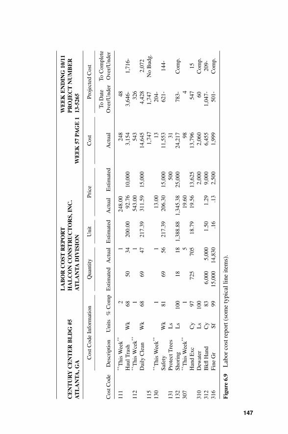
P1: OTA/XYZ P2: ABC


CE

NT

UR

YC

EN

TE

RB

LD

G#5

AT

LA

NT

A,G

A

LA

BO

RC

OST

RE

PO

RT

HA

LC

ON

CO

NST

RU

CT

OR

S,IN

C.

AT

LA

NT

AD

IVIS

ION

WE

EK

57PA

GE

1

WE

EK

EN

DIN

G10

/11

PR

OJE

CT

NU

MB

ER

13-5

265

Cos

tCod

eIn

form

atio

nQ

uant

ityU

nit

Pric

eC

ost

Proj

ecte

dC

ost

ToD

ate

ToC

ompl

ete

Cos

tCod

eD

escr

iptio

nU

nits

%C

omp

Est

imat

edA

ctua

lE

stim

ated

Act

ual

Est

imat

edA

ctua

lO

ver/

Und

erO

ver/

Und

er

111

∗∗T

his

Wee

k∗∗2

124

8.00

248

48H

aulT

rash

Wk

6850

3420

0.00

92.7

610

,000

3,15

43,

646-

1,71

6-11

2∗∗

Thi

sW

cek∗∗

11

543.

0054

332

6D

aily

Cle

anW

k68

6947

217.

3931

1.59

15,0

0014

,645

4,42

82,

072

115

1,74

71,

747

No

Bud

g.13

0∗∗

Thi

sW

eek∗∗

11

13.0

013

204-

Safe

tyW

k81

6956

217.

3920

6.30

15,0

0011

,553

621-

144-

131

Prot

ectT

rees

Ls

500

3113

2Sh

orin

gL

s10

018

181,

388.

881,

345.

3825

,000

24,2

1778

3-C

omp.

307

∗∗T

his

Wee

k∗∗1

519

.60

984

Han

dE

xcC

y97

725

705

18.7

919

.56

13,6

2513

,796

547

1531

0D

ewat

erL

s10

02,

000

2,06

060

Com

p.31

2B

kflH

and

Cy

836,

000

5,00

01.

501.

299,

000

6,45

51,

047-

209-

316

Fine

Gr

Sf99

15,0

0014

,830

.16

.13

2,50

01,

999

501-

Com

p.

Fig

ure

6.9

Lab

orco

stre

port

(som

ety

pica

llin

eite

ms)

.

147

P1: OTA/XYZ P2: ABC



sufficient information is available to the contractor at the time of bid to allowrelatively precise definition of these job-related indirect costs. The R. S. Meansmethod of developing overhead and profit represents a percentage rate ap-proach that incorporates a charge into the estimate to cover overhead on a lineitem-by-item basis. This is essentially a variation of the flat rate application.

FIXED OVERHEAD

Whereas the project indirect charges are unique to the job and should beestimated on a job-by-job basis, home office overhead is a more or less fixedexpense that maintains a constant level not directly tied to individual projects.In this case, the application of a percentage rate to prorate or allocate homeoffice expense to each project is accepted practice, since it is not reasonable totry to estimate the precise allocation of home office charges to a given project.Rather, a percentage prorate or allocation factor is used to incorporate supportof home office charges into the bid.

The calculation of this home office overhead allocation factor isbased on:

1. The general and administrative (G&A) (home office) expenses incurredin the past year.

2. The estimated sales (contract) volume for the coming year, and3. The estimated gross margin (i.e., markup) for the coming year.

This procedure is illustrated in the following example (Adrian, 1978).

Step 1: Estimate of Annual Overhead (G&A Expense)Last year’s G&A $270,00010% inflation 27,000Firm growth 23,000Estimated G&A $320,000

Step 2: Estimate of $ of Cost Basis for AllocationEstimated volume $4,000,000Gross margin 20% = $800,000Labor and material $3,200,000

Step 3: Calculate Overhead PercentOverhead Est.

Labor and Materials= $320,000

$3,200,000= 10%

Step 4: Cost to Apply to a Specific ProjectEstimated labor and material costs $500,000Overhead to apply (@ 10%) 50,000Total $550,000

P1: OTA/XYZ P2: ABC


CONSIDERATIONS IN ESTABLISHING FIXED OVERHEAD 149

In the example, the anticipated volume for the coming year is $4,000,000.The G&A expense for home office operation in the previous year was$270,000. This value is adjusted for inflation effects and expected expansionof home office operations. The assumption is that the overhead allocationfactor will be applied to the direct labor and materials costs. These directcosts are calculated by factoring out the 20% gross margin. Gross margin, inthis case, refers to the amount of overhead and profit anticipated.

Direct costs amount to $3,200,000. The $320,000 in G&A costs to berecovered indicate a 10% prorate to be applied against the $3,200,000 ofdirect costs. This means that an overhead amount of $50,000 would be addedto a contract bid based on $500,000 of direct cost to provide for G&A costrecovery. The profit would be added to the $550,000 base recovery amount.

CONSIDERATIONS IN ESTABLISHING FIXED OVERHEAD

In considering costs from a business point of view, it is common to categorizethem either as variable costs or fixed costs. Variable costs are costs directlyassociated with the production process. In construction, they are the directcosts for labor, machines, and materials as well as the field indirect costs (i.e.,production support costs). These costs are considered variable since they varyas a function of the volume of work underway. Fixed costs are incurred at amore or less constant rate independent of the volume of work-in-progress. Inorder to be in business, a certain minimum of staff in the home office, space forhome office operations, telephones, supplies, and the like must be maintained,and costs for these items are incurred. These central administrative costs aregenerally constant over a given range of sales/construction volume. If volumeexpands drastically, home office support may have to be expanded also. Forpurposes of analysis, however, these costs are considered fixed or constantover the year. Fixed costs are essentially the general and administrative costsreferred to earlier.

The level of G&A (fixed) costs can be estimated by referring to the actualcosts incurred during the previous year’s operation. The method of projectingfixed overhead as a percentage of the estimated total direct costs projectedfor the coming year is widely used. Since the fixed overhead incurred in theprevious year is typically available as a percentage of the previous year’s totalsales volume, a simple conversion must be made to reflect it as a percentageof the total direct cost. The formula for this conversion is:

PC = PS

(100 − PS)

wherePC = percentage applied to the project’s total direct cost for the coming

year, and

P1: OTA/XYZ P2: ABC



PS = percentage of total volume in the reference year incurred as fixedor G&A expense.

If, for instance, $800,000 is incurred as home office G&A expense in areference year in which the total volume billed was $4,000,000, the P valuewould be 20% ($800,000/$4,000,000 x 100). The calculated percentage tobe added to direct costs estimates for the coming year to cover G&A fixedoverhead would be:

PC = 20

100 − 20= 25%

If the direct cost estimate (e.g., labor, materials, equipment and field indi-rect costs) for a job is $1,000,000, $250,000 would be added to cover fixedoverhead. Profit would be added to the total of field direct and indirect costsplus fixed overhead. The field (variable) costs plus the fixed overhead (G&A)charge plus profit yield the bid price. In this example, if profit is included at10%, the total bid would be $1,375.000. It is obvious that coverage of thefield overhead is dependent on generating enough billings to offset both fixedand variable costs.

Certain companies prefer to include a charge for fixed overhead that ismore responsive to the source of overhead support. The assumption here isthat home office support for management of certain resources is greater orsmaller, and this effect should be included in charging for overhead. Forinstance, the cost of preparing payroll and support for labor in the field maybe considerably higher than the support needed in administering materialsprocurement and subcontracts. Therefore, a 25% rate for fixed overhead isapplied to labor and equipment direct cost, while a 15% rate on materials andsubcontract costs is used. If differing fixed overhead rates are used on varioussubcomponents of the field (variable) costs in the bid, the fixed overheadcharge will reflect the mix of resources used. This is shown in Table 6.3 inwhich a fixed rate of 20% on the total direct costs for three jobs is comparedto the use of a 25% rate on labor and equipment and a 15% rate on materialsand subcontracts.

It can be seen in Table 6.4 that the fixed overhead amounts using the25/15% approach are smaller on jobs 101 and 102 than the flat 20% rate.This reflects the fact that the amount of labor and equipment direct coston these projects is smaller than the materials and subcontract costs. Theassumption is that support requirements on labor and equipment will also beproportionately smaller. On job 102, for instance, it appears that most of thejob is subcontracted with only $200,000 of labor and equipment in house.Therefore, the support costs for labor and equipment will be minimal, and thebulk of the support cost will relate to management of materials procurementand subcontract administration. This leads to a significant difference in fixedoverhead charge when the 20% flat rate is used, as opposed to the 25/15%modified rates (i.e., $440,000 versus $350,000).

P1: OTA/XYZ P2: ABC


BREAKEVEN ANALYSIS 151

TABLE 6.4 Comparison of Fixed Overhead Rate Structures

20% on DirectCosts

25% on Labor& Equipment;

15% onMaterials and

Subs

Labor and Equipment $800,000 160,000 200,000Job 101 Materials and subcontracts 1,200,000 240,000 180,000

400,000 380,000

Labor and Equipment 200,000 40,000 50,000Job 102 Materials and subcontracts 2,000,000 400,000 300,000

440,000 350,000

Labor and Equipment 700,000 140,000 175,000Job 103 Materials and subcontracts 700,000 140,000 105,000

280,000 280,000

On job 103, the fixed overhead charge is the same with either of the ratestructures, since the amount of labor and equipment cost is the same as theamount of the materials and subcontract cost.

It should be obvious that in tight bidding situations use of the stylizedrate system, which attempts to better link overhead costs to the types ofsupport required, might give the bidder an edge in reducing the bid. Ofcourse, in the example given (i.e., the 25/15% rate versus 20%), the 20%flat rate would yield a lower overall charge for fixed overhead on labor-and equipment-intensive jobs. The main point is that the charge for fixedoverhead should be reflective of the support required. Because the multiplerate structure tends to reflect this better, some firms now arrive at fixedoverhead charges by using this approach rather than the flat rate applied to totaldirect cost.

BREAKEVEN ANALYSIS

Both variable and fixed costs (as described in the previous section) mustbe recovered by billing to the client. A certain percentage of each billeddollar must cover the variable costs incurred, while another portion of thebilled dollar must cover the fixed overhead costs (general and administrativeexpense). This is shown conceptually in Figure 6.10. If billings exceed acertain amount (a certain level of volume is achieved), profit will be generatedby the billings. However, up to a certain level of billings, all of the dollarsbilled are essentially covering the combined fixed and variable costs. Thepoint at which billed volume is equal to the fixed and variable cost incurredto generate it is called the breakeven point.

P1: OTA/XYZ P2: ABC



Dollaramount

billed

Profit

% of billed amount to coverfixed overhead (G&Aexpenses)

% of billed amount to covervariable costsassociated withproject

i.e., chargesby subcontractors,by vendors formaterials, payrolland equipment

charges

Figure 6.10 Distribution of Billed Dollars to Cover Costs Incurred.

To better understand this concept, consider the portion of each dollarbilled that is to be applied to fixed overhead. As described in the previoussections, the amount of fixed overhead (G&A) expense is normally projectedfrom the previous year’s operations. Assume that the amount of fixedoverhead corrected for inflation and expanded operations for the presentyear is $400,000. Assume further that the percentage of each billed dollarrequired to cover operations costs is 80%. This means that 80 cents of eachbilled dollar is expended on variable costs. Twenty cents is left to coverfixed overhead. How many dollars must be billed to cover the $400,000 ofprojected fixed overhead? Based on 20 cents per dollar for fixed overhead, theminimum amount of billings required to cover the projected G&A expensewould be $400,000 divided by 0.20, or $2 million. That is, until $2 millionhas been billed to clients, the fixed overhead has not been recovered. If morethan $2 million is billed over the year, profit will be generated at the rate of20 cents on the dollar for every dollar in excess of $2 million. On the otherhand, if the volume of billings falls below $2 million, the fixed overhead willnot be fully covered, and a loss will occur. A graphical representation of thissituation is given in Figure 6.11. It is this point, at which billings just coverfixed and variable costs, that is called the breakeven point. The chart shownis referred to as a breakeven chart. The slope of the variable cost line is$0.80/billed dollars. The variable cost line starts on the Y-axis at the level ofprojected fixed cost (i.e., projected G&A costs for the year). The broken lineshows the billings amount profile. As the amount billed increases, the variablecosts also increase. At $2 million billed, the “billings amount” line intersectsthe total cost line (fixed + variable), indicating that billings equal fixed andvariable costs. The chart is based on a few simple equations. At the breakevenpoint, billings volume (BV) must equal fixed costs (FC) plus variablecosts (VC).

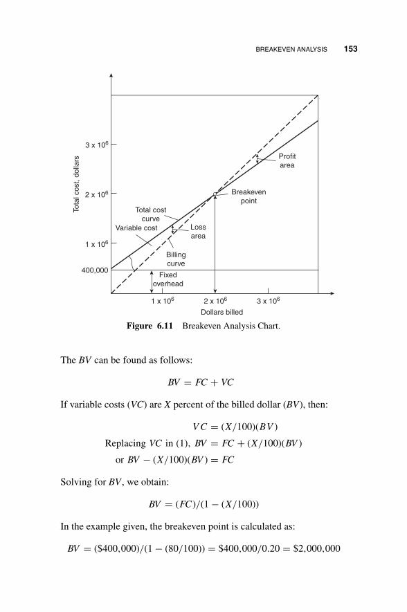
P1: OTA/XYZ P2: ABC


BREAKEVEN ANALYSIS 153

3 x 106

3 x 106

2 x 106

2 x 106

1 x 106

1 x 106

400,000

Dollars billed

Fixed

overhead

Billing

curve

Lossarea

Variable cost

Total cost

curve

Breakeven

point

Profitarea

Tota

l cost, d

olla

rs

Figure 6.11 Breakeven Analysis Chart.

The BV can be found as follows:

BV = FC + VC

If variable costs (VC) are X percent of the billed dollar (BV), then:

V C = (X/100)(BV )

Replacing VC in (1), BV = FC + (X/100)(BV )

or BV − (X/100)(BV ) = FC

Solving for BV , we obtain:

BV = (FC)/(1 − (X/100))

In the example given, the breakeven point is calculated as:

BV = ($400,000)/(1 − (80/100)) = $400,000/0.20 = $2,000,000

P1: OTA/XYZ P2: ABC



BASIC RELATIONSHIPS GOVERNING THE BREAKEVEN POINT

Several relationships are clear from a consideration of the breakeven chart inFigure 6.11 and the supporting equations.

Lowering the fixed overhead amount will move the breakeven point to theleft (reduce the volume require) if the variable cost percentage is constant.If the fixed overhead amount in the example is reduced to $300,000, thenew breakeven point will be $300,000/0.20 = $1,500,000. This is shown inFigure 6.12.

If the percentage of each billed dollar required to cover variable costs isreduced, the breakeven point volume is reduced. This is obvious, since thetotal cost curve slope is reduced, while the billings curve slope is constant (i.e.,always 45 degrees). If in the example the fixed overhead cost is $400,000 asoriginally stated, but the variable cost percentage is 75%, the new breakevenpoint volume will be $1,600,000. This is shown in Figure 6.13.

Below the breakeven point, the loss associated with a given constructionvolume is the difference between the total cost curve and the billings curve.

Total cost

curve with$400,000 fixed

overhead

Total cost

curve with

$300,000 fixedoverhead

Loss

Breakeven

point with

$300,000 fixed

overhead

Breakeven point with

$400,000 fixedoverhead

Profit

400,000

300,000

.5 1

Billed amount (in millions of dollars)

1.5 2

Tota

l cost

Figure 6.12 Variation in breakeven point based on reducing fixed overhead.

P1: OTA/XYZ P2: ABC



Total cost curve

Loss

Profit

Variable costs

0.75

Fixed O/H = $400,000

Billed amount (in millions of dollars)

Tota

l cost

.5 1 1.5 2

Figure 6.13 Variation in breakeven point based on reducing variable cost.

Above the breakeven point, this difference represents the profit associatedwith a given volume. These relationships are illustrated in Figure 6.11.


1. Given the following cost expenditures (see Table P6.1) for a small ware-house project (to include direct and indirect changes):A. Calculate the peak financial requirement.B. Sketch a diagram of the overdraft profile.C. What would be the impact on the maximum overdraft of giving the

contractor a $25,000 mobilization payment? (Show calculation.)Assumptions:� The markup for this project is 12%.� Retainage is 10% throughout project.� Finance charge is 1.5% per month.

P1: OTA/XYZ P2: ABC



� Payments are billed at the end of the month and are received one monthlater.

� All expenses are paid immediately.

TABLE P6.1 Monthly Cost

Month 1 2 3 4Monthly cost∗ 69,000 21,800 17,800 40,900

∗ Direct cost + indirect cost

2. The contract between Ajax Construction Co. and Mr. Jones specifies thatthe contractor will bill Mr. Jones at the end of each month for the amountof work finished that month. Mr. Jones will then pay Ajax a specifiedpercentage of the bill the same day. The accumulated retainage is to bepaid one month after project completion. The latest cumulative billingwas $5 million, of which Ajax has actually received $4.5 million. Theproject is to be finished two months from now. Ajax estimates the billfor the remaining two months will be $100,000 and $50,000. Mr. Jones,being short of cash at present, proposed the following alternative: Ratherthan follow the contract and make the three payments required, he willmake one final payment (for the two months’ work plus the retainage)five months from now. Mr. Jones will also pay a 4% monthly interest ratebecause of the delay in payment.

Find what would be the total final payment according to the actualcontract and the new final payment according to the new proposal. Shouldthe contractor accept the new proposal? Why?

3. Can you think of additional strategies to bring closer the payments anddisbursements curves (as discussed for Figure 6.8)?

4. Direct costs of a project are shown on the following bar chart(see Table P6.2). Assume $500 per month indirect cost and 10% re-tainage with payment time lag of one month.

Calculate the project’s net cash flow for a 10-percent markup. Estimatethe proper markup for 1%, 1.5%, and 2% rate of return per month, usingmethods described in Chapter 7.

5. Given the following cost expenditures (see Table P6.3) for a small bridgejob to include direct and indirect charges (but not bank interest):A. Calculate the peak financial requirement.B. Sketch a diagram of the overdraft profile.Assumptions:� The markup for this project is 8%.� Finance charge is 1% per month.

P1: OTA/XYZ P2: ABC



TABLE P6.2 Project Bar Chart

MonthActivity

54321

1. Survey $2,000

2. Mobilization $1,200

3. Trench $3,000 $6,000

4. Lay pipe $3,000

5. Concrete $500 $500

6. Backfill $500

7. Move out $500

8. Prepare valves $1,000

9. Install valves $1,000

10. Test $1,500

� Retainage is 6% throughout project.� Payments are billed at the end of the month, and are received one month

later.

TABLE P6.3 Monthly Costs for Bridge Job

Month 1 2 3Monthly cost∗ 29,000 48,900 16,400

∗ Direct cost + indirect cost

6. A contractor is preparing to bid for a project. He has his cost estimate andthe work schedule. Table P6.4 gives his expected expenses and their timeof occurrence. Other expenses such as insurance, bonds, and payroll taxesare included. For simplicity of analysis, he assumed that all expenses arerecognized at the end of the month in which they occur.

The contractor is planning to add 10% to his estimated expenses tocover profits and office expenses. The total will be his bid price. Heis also planning to submit for his progress payment at the end of eachmonth. Upon approval the owner will subtract 5% for retainage and paythe contractor one month later. The accumulated retainage will be paid tothe contractor with the last payment (i.e., at the end of month 13). Whatis the peak financial requirement and when does it occur?

P1: OTA/XYZ P2: ABC



TABLE P6.4 Table of Expenses

MonthMobilization /

DemobilizationSubcon-tractors Materials Payroll Equipment

FieldOverhead

0 $40,000 $0 $0 $0 $0 $01 0 10,000 10,000 10,000 20,000 1,0002 0 30,000 20,000 15,000 10,000 5,0003 0 30,000 30,000 20,000 20,000 6,0004 0 40,000 30,000 20,000 30,000 6,0005 0 50,000 40,000 40,000 20,000 6,0006 0 50,000 40,000 40,000 15,000 6,0007 0 40,000 30,000 40,000 10,000 6,0008 0 40,000 10,000 20,000 10,000 6,0009 0 70,000 10,000 10,000 10,000 6,000

10 0 30,000 5,000 5,000 10,000 6,00011 0 30,000 5,000 5,000 5,000 6,00012 20,000 50,000 0 5,000 5,000 5,000

Total $60,000 $470,000 $230,000 $230,000 $165,000 $65,000

Total cost = 60,000 + 470,000 + 230,000 + 230,000 + 165,000 + 65,000 = $1,220,000Profit plus overhead = (10%) (total cost) = $122,000Bid price = total cost + profit + overhead = $1,342,000

7. Based on the definition of fixed cost, list costs in the main office that arenot really fixed, and field office costs that are fixed.

8. Categorize the following costs as (a) direct, (b) project indirect, or (c)fixed overhead.� Labor� Materials� Main office rental� Tools and minor equipment� Field office� Performance bond� Sales tax� Main office utilities� Salaries of managers, clerical personnel, and estimators

9. The following data are available on Del Fabbro International, Inc.What bid price should be submitted to insure proper coverage of fixedoverhead?� The fixed (home office) overhead for the past year was $365,200.� Total volume was $5,400,000.

P1: OTA/XYZ P2: ABC



� Del Fabbro uses a profit markup of 10%.� The estimating department has indicated that the direct and project

(field) indirect costs will be $800,000.� Assume a 5% inflation factor and a 12% growth factor.

10. Using the data of the previous problem, calculate the breakeven point forDel Fabbro International in the present year.

P1: OTA/XYZ P2: ABC


CHAPTER 7

TIME VALUE OF MONEY ANDEVALUATING INVESTMENTS

INTRODUCTION

The topics that we have covered so far do not consider the fact that the use ofmoney costs money. If you use your own money you forgo any interest youmight achieve by investing it. If you need to borrow it, you must pay for theuse of the money. The time required to make or spend money has not beenaddressed so far in our discussion of financial management. In fact, the cost ofmoney and the time during which money is tied up in any business decisionprocess are crucial factors. To illustrate this point, consider the followingcases.

1. Assume that you are buying a new car. The purchase price is $26,050,and you plan to pay this amount over a 60-month time period. Oneoption involves a $1,000 cash discount and a loan at the rate of 6.94%.A second option is to finance the car at with a 5.9% interest loan, but nodiscount? Which option is better? (Answer: the two are the same—you’dpay around $500 per month taking either one).

2. What will be the balance of your mutual funds account when you retireat 65 if you are 25 now and begin depositing $100 per month rightaway? Assume a 12% annual interest. (Answer: Over a million dollars).

3. What would be the balance of the same account, if you begin savingwhen you are 35? (Answer: $350,000).

4. What is the down payment for a house worth $250,000, if you can geta 30-year fixed interest rate of 7.50% and want to cap the payments to$1,500 per month? (Answer: Exactly $35,473.56).

161



P1: OTA/XYZ P2: ABC


162 TIME VALUE OF MONEY AND EVALUATING INVESTMENTS

Similar decisions are frequently faced by any business enterprise. Shouldmy company continue leasing this building or should it build a new one?Which piece of equipment from among these choices should I choose? Is this3-year project with a profit of $1,000,000 better than this other that can befinished in a year with a $250,000 profit?

Engineering Economy considers the time and cost of borrowing as theyrelate to these and many other questions involving money as a construc-tion resource. In this chapter, we will discuss the time value of money.The management of expensive, long-term construction projects definitelyrequires a thorough understanding of the principles and techniques discussedhere. Money management on complex long term projects is too impor-tant to be dealt with using “horseback questimates.” Engineering Econ-omy is increasingly useful even for small, personal decisions like thosedescribed above. Calculators, software, and thousands of websites providesupport in dealing with the topics covered here. Construction managers musthave a very good working understanding of the concepts discussed in thischapter.

TIME VALUE OF MONEY

If someone asked you to decide between receiving $1,000 right now or re-ceiving it 1 year from now, wouldn’t you choose to get the money right away?You could invest the money, pay back a debt, or simply keep it until there isa good reason to spend it.

If you were lending $1,000 for 1 year to a perfect stranger, wouldn’t youexpect to receive more than $1,000 back? After all, you could have investedthis money in a Certificate of Deposit or in your own business. The borrowerwould have had the potential to invest this money, while you’d have beendeprived from this possibility. In short, it is reasonable that anyone lendingmoney asks for “rent,” and anyone borrowing money must expect to pay“rent” for its use. This rationale is at the center of the concepts presented inthis chapter.

INTEREST

Interest is the fee that a lender charges for the use of their money. Fromthe borrower’s viewpoint, it is the “rent” paid for the use of someone else’smoney. Normally, it is directly proportional to the amount of money loanedor borrowed. That is, a $2,000 loan almost always earns twice the interestamount of a $1,000 loan. Interest is also proportional to the time that moneyhas been loaned or borrowed. A three-year loan earns more interest thana single year loan for the same amount.

P1: OTA/XYZ P2: ABC


SIMPLE AND COMPOUND INTEREST 163

The money that one dollar earns for each unit of time that it is loaned iscalled its interest rate. This rate is expressed as a percentage: If $20.00 earns$2.40 over a year, then the interest rate in this case is $2.40 / $20.00 = 0.12,or 12% per year. It is so common to deal with interest rates that often theyare referred simply as “interest,” with the “rate” being implied by the contextof the situation. To avoid confusion, the money earned by charging interestis frequently called total interest. It should be easy to notice which of theseterms is being used in a specific context. If the interest refers to a percentage,then the complete term should be interest rate.

The interest rate established for any business transaction is of paramountimportance. Let’s suppose that you take a $200,000 mortgage loan to pur-chase a house. If you agree to pay back the loan over 30 years at a 15%interest1, your monthly payment toward repaying the loan will be $2,528.89.If the interest is 7%, your payment would be $1,330.60, approximately halfthe previous amount. While the total interest paid over the 30 years wouldbe $710,399.70 at 15%, it would be $279,017.80 at 7%. In both cases,you end up paying more for interest than the original borrowed amount.But, why would anyone agree to pay 15% instead of 7%? The degree ofinvestment risk, the inflation rate, and the stability of the market wherethe money will be used are important factors determining the interest rateof a particular loan. For instance, lenders charge higher interest rates toborrowers with a higher risk of defaulting on the loan. Other factors canalso influence rates, such as the level of competition among lenders andthe cost of the money to them (since often lenders, in turn, borrow theirmoney).

SIMPLE AND COMPOUND INTEREST

There are two fundamentally different ways to compute interest. Let us sup-pose that you need $10,000, which you will pay back at the end of 3 years,plus all the interest accumulated over the 3 years. If you have to pay a 10%interest rate, how much money will you have to pay back? The original bor-rowed amount, or loan principal, is $10,000. The total interest, as previouslymentioned, depends on the principal, the time that the money was borrowed,and the interest rate. Moreover, it depends on the type of interest: whether itis simple or compound, as discussed here.

Simple Interest. You ask Uncle Fudd to lend you the $10,000. He agrees toallow you to pay simple interest, as a concession to one of his favorite familymembers. Paying simple interest means that you pay interest on the principalbut not on the interest accumulated from previous periods. Therefore, yourdebt at the end of each year is computed as shown in Table 7.1.

1 In this context, it is assumed that 15% means 15% per year.

P1: OTA/XYZ P2: ABC



TABLE 7.1 Simple Interest Calculation

Year n Base for applying i Interest for period Total owed, F

0 (now) 10,0001 10,000 10,000 × 0.10 = 1,000 11,0002 10,000 10,000 × 0.10 = 1,000 12,0003 10,000 10,000 × 0.10 = 1,000 13,000

For simple interest, the future value Fn of a principal P borrowed over nperiods at an interest rate i can be computed as Fn = P + P ∗ i ∗ n, or moredirectly,

Fn = P × (1 + i × n)

In this case, we can compute F3 = 10,000 × (1 + 0.10 × 3) = 10,300without developing the table above.

Compound Interest. You decide to use a bank to borrow the $10,000 insteadof asking your uncle. Banks never use simple interest to compute your debt.Instead, the interest owed after each time period is computed by adding thetotal interest accumulated from previous periods to the loan principal, andthen multiplying this total by the interest rate. The computations in Table 7.2help to illustrate how this process works.

Using the same notation as for simple interest above, you can see that:

Fn = P × (1 + i)n

Using this formula, we can find F3 directly:

F3 = 10,000 × (1 + 0.10)3 = 13,310

The formula above also works in the opposite direction. One can find theprincipal that would result in a future value, F, after n periods at an interestrate of i using the formula:

P = Fn/(1 + i)n

TABLE 7.2 Compound Interest Calculation

Year n Base for applying i Interest for period Total owed, F

0 (now) 10,0001 10,000 10,000 × 0.10 = 1,000 11,0002 11,000 11,000 × 0.10 = 1,100 12,1003 12,100 12,100 × 0.10 = 1,210 13,310

P1: OTA/XYZ P2: ABC


NOMINAL AND EFFECTIVE RATE 165

The P found here is usually called the Present Value, P, of the futureamount, F.

Compound interest is more logical and equitable than simple interest. Whywould the interest accumulated to date be exempt from consideration, as insimple interest? In fact, as you can appreciate in the mortgage loan exampleof the previous section, many times the earned interest is higher than a loan’sprincipal. Simple interest is never used for business transactions.

NOMINAL AND EFFECTIVE RATE

A lender could advertise in big letters a 1% interest rate and then add in verysmall letters that it refers to the monthly rate, not the annual rate as manypeople would assume. Technically, the lender would be telling the truth: aninterest rate can refer to any time unit, from seconds to decades, but manypeople would be deceived by such advertising strategy. To protect consumers,Congress passed in 1968 the Truth in Lending Act, which, among other issues,requires that lenders clearly indicate interest rates as an annual percentageof each received dollar. This Annual Percentage Rate (APR) also includesupfront commissions and fees converted to equivalent annual percentages.

Requiring that lenders disclose their APR was an important step for con-sumer protection. However, an APR can still be misleading. The APR simplyadds the interest rates charged in 1 year, instead of compounding these in-termediate periods. If your credit card charges 1% per month, then its APRis (1%/month) × (12 months/year) = 12%. This is the nominal interest rateof your card, but it is not its effective interest rate. If you have $10,000 incredit card charges, the APR suggests that you will owe $10,000 × (1.12) =$11,200 a year from now (assuming that you make no payments during theyear). However, since the card company computes financial charges everymonth, you would owe $10,000 × (1 + 0.01)12 = $11,268.25 at the end ofthe year, using the compound formula for F that we examined in the previ-ous section. The $68.25 difference is substantial, and perfectly legal for thecredit card company to charge. Almost all credit cards charge interest by theday, which means that the total annual interest that you’d owe in the aboveexample almost certainly would be $10,000 × (1 + 0.12/365)365 = $11,274.75.

It is possible to find the effective annual rate that you pay on a loan (usuallycalled its Annual Percentage Yield, or APY) if you know its APR and thenumber of times per year that the interest is compounded. The followingformula finds a loan’s APY when its APR and the number of times per yearthat the APR is compounded (the C in the formula below) are known.

APY = (1 +AP R/C )C − 1

If the interest is compounded monthly, then C = 12, the number of monthsin a year.

P1: OTA/XYZ P2: ABC



In the previous example, APR = 12% compounded monthly. Its APY is:

APY = (1 + 0.12/12)12 − 1 = 0.126825 or 12.6825%

An APY is not too different from its APR compounded C times, but aseemingly small difference can be significant. If you take $100,000 to repayafter 15 years at i = 12.0000% and at12.6825%, the future amounts owed are:

For i = 12.0000% : F = $100,000 × (1 + 0.120000)15 = $547,356.57For i = 12.6825% : F = $100,000 × (1 + 0.126825)15 = $599,580.20

The difference of $52,223.63 is due exclusively to the difference betweenAPR and APY.

EQUIVALENCE AND MARR

If you have an offer to receive $100 now or $110 a year from now, whichoption would you choose? Assume that you have enough resources to thinkabout this offer in terms of investing the money, as opposed to spending it onsome “spur of the moment” purchase. Even with enough money to subsist,many people will choose the $100 now, for the reasons previously discussedin the section on the time value of money. But, what happens if instead of$110, you are offered $500 a year from now? What if the future amountoffered is $400? Or $300? Or $150? Deciding which offer to take gets moretricky. It is quite possible that you’d choose the $500 a year from now, butsome of the lower amounts would probably be attractive enough to preferthem over the $100 offered now in this hypothetical example.

Let us take this mental exercise to the point that you are offered an amountthat is just high enough to make you indifferent to having it now or in thefuture. The two amounts are said to be equivalent to you. The “you” in theprevious sentence is important. Someone else could have a different idea ofwhat is equivalent to $100 now. You would certainly require a higher amounttwo years from now than what you would get a year from now to declareequivalence in preference.

Equivalence is usually considered in terms of interest rates instead of totalinterest. If your equivalent amount for $100 is $150 received a year from now,then the total interest would be $150 − $100 = $50. The interest rate wouldbe $50 / $100 = 50%. This particular interest rate is called your Minimum At-tractive Rate of Return, or MARR. In an actual business environment, MARRis not found as arbitrarily as shown here. If you are in heavy construction andin your experience a reasonable Return on Equity is 20%, then you could notaspire to a 50% MARR. If you are paying 10% interest on your borrowedmoney, then your MARR cannot be less than 10%. If your MARR is less

P1: OTA/XYZ P2: ABC


IMPORTANCE OF EQUIVALENCE 167

than 10%, you would lose money when borrowing at 10%—you would paymore borrowing costs than you would make on the return from your MARR.If your Uncle Fudd makes 25% on his money and is willing to let you investin his company, then you could establish this rate as your MARR. If UncleFudd can consistently offer you 25%, why should you accept less?

Computing MARR is a sensitive and sophisticated issue for any company,and we will not cover this topic in detail here. However, keep in mind thatwhen we use an interest rate i in any problem here, usually this rate is theMARR for at least one of the stakeholders in the problem.

DISCOUNT RATE

What we have called so far interest rate is sometimes called discount rate.When we discussed the concept of interest, we approached it from the per-spective of someone beginning with an amount P (at time present) and endingin the future with an amount F. When we know the value in the future of agiven sum and want to know what its value in today’s currency would be, onespeaks of discounting the future amount, F, to the present at some “i” value.We want to find P given F. P is equivalent to the known value F when F isdiscounted using the formula P = Fn / (1 + i)n. This formula is the inverse ofFn = P × (1 + i)n.

The equivalence of P and F can be extended to include several Fs. Letus suppose that we are offered $55.00 a year from now and $60.50 2 yearsfrom now. If our MARR is 10%, we can find that the first future amountis equivalent to a present amount of $55.00/(1.10)1 = $50, and the secondamount is equivalent to $60.50/(1.10)2 = $50 now. We will be willing toaccept $50 + $50 = $100 now, instead of the two amounts in the future.

IMPORTANCE OF EQUIVALENCE

Equivalence is a very handy way moving values such as P and F from pointto point in time. For instance, we can use this principle to determine paymentor payment required to purchase merchandise on credit. If a seller offers a10% credit, we can purchase a $100 music player and arrange to pay for it intwo payments, one of $55.00 a year from now and another of $60.50 2 yearsfrom now, since these two payments are equivalent to $100 today, as you sawpreviously. The seller will be willing to let us take home the merchandisewith our written promise to pay back these two amounts above the specifiedpoints in time. (More likely, we would prefer to pay two equal payments of$57.62—such equal amounts are called annuities, as we will discuss later)

The concept of equivalence is central to understanding the rest of thischapter, so let us work through a final mental exercise about this concept. Themusic you listen in your earphones could sound exactly as loud to you as the

P1: OTA/XYZ P2: ABC



systems in your car or living room, although the earphones are, in decibels,much quieter than the car or room systems. In our money equivalence, thedollar amount now is the decibel volume delivered right in your ears; thedistance between you and the speakers of the other systems is the timebetween receiving different dollar amounts. And equivalence is equivalence.You can be as happy quietly listening to a good pair of earphones as to agood set of speakers. You can be equally satisfied receiving one dollar nowas opposed to $1.10 a year from now or $1.21 2 years from now, providedthat your MARR is 10%.

INFLATION

The cost of goods and services tend to increase over time. This phenomenonis called inflation and is subject to much consideration by macroeconomists.The purchasing power of a dollar is progressively reduced by inflation, and,therefore, a year from now we may need $105.00 to purchase the merchandisethat we can buy today for $100.00. In 2 years, we would have to pay $110.25for the same article (more than $110.00, because the inflation for the secondyear is 105% of $105, not of $100). In general, an inflation rate of “f ” increasesthe cost of goods over n periods in accordance with the formula F = P ×(1 + f )n. You can see that this formula is similar to our familiar F and Prelationship when applying a compound interest rate i over n periods.

Inflation undercuts the practical effect of charging interest. An investorcharging a 5% interest on $100 for a year should be able to purchase anadditional $5 worth of goods at the end of the year. If inflation runs at anannual 5%, this investor would not be able to purchase any additional goods,since a $100 today would cost $105 in a year. Inflation would have offset allthe real gains from the interest collected.

The effective interest rate “ i’,” that is, what an investor is actually makingafter considering an inflation rate of f is found as follows:

i ′ = [(1 + i)/(1 + f )] − 1

If i = f , as in the previous example, the effective interest rate is zero.Applying the formula above, a nominal interest of 9% in an economy with3% inflation would yield an effective interest rate of 5.825%. This result isclose to the difference between the nominal interest rate and the inflation rate:9% – 3% = 6%. They are not the same—and worse, this incorrect computationunderestimates the effect of inflation. An investor would believe that moneywill yield 6.000% when in fact it is yielding less, 5.825%.

Inflation is not considered in many engineering economy analyses, becauseall costs, including those charged by the investor, can be passed through tothe purchaser or client. That is, as prices and costs raise, the selling price isadjusted to pass the inflation increase on to the purchaser. As an example,

P1: OTA/XYZ P2: ABC


CASH FLOW DIAGRAMS 169

consider the economic analysis of a new toll highway. The analysis mustaddress a period of 15 or 20 years, and estimating the inflation for suchan extended period would be futile. Tolls, however, can be expected to risewith inflation, and their price in 20 years is immaterial as long as the analysisclarifies that figures are in today’s “constant dollars.” The toll will be adjusted(increased) to pass inflation for operation and other costs through to the user.Some financial arrangements, however, are fixed and cannot be adjusted overtime for inflation. A typical example is the case of a 30-year fixed interesthome mortgage loan.

SUNK COSTS

We have discussed situations in which all factors involved in the businessdecision occur in the present or the future. Engineering economy is notconcerned with past costs or lost benefits. Any cost in the past is called a sunkcost, and as the name implies, it should be irrelevant to the decision at hand.

Let us illustrate the concept of sunk costs with the following scenario. Youpurchased a $2,000 brand new laptop computer 3 months ago. However, anew model with the same features is available now for $1,000. Cousin Elmeroffers you $1,200 for the old computer. Should you sell the old computer andpurchase the new model?

The cost of the original laptop is irrelevant to the decision of keepingor selling it. Many people have difficulty in selling a possession at a losscompared to the price they paid for it. In this case, keeping the computerwould avoid the sense of having made a bad decision by purchasing it inthe first place. But, that is faulty logic. The key point to consider should bewhether you are better off by your decision. What is relevant is that sellingthe computer would give you an extra $200, and keeping it would preventyou from realizing this profit.

There could be other factors not mentioned previously that could swayyour decision toward keeping the computer. Maybe the laptop was a gift ofyour dear Uncle Dewey, and you don’t want to offend him by selling it. Or, nothaving the hassle of setting up the new computer is worth more than the extra$200. These are true considerations, not easily quantifiable. But in summary,using engineering economy principles, you should sell your current laptopand buy the new model given the scenario of this example.

CASH FLOW DIAGRAMS

So far, we have used only words to describe our examples. In most realsituations, this is a cumbersome approach at best, especially when comparedto using the power and simplicity of graphics to convey information. Cashflow diagrams are a graphical means used to describe engineering economy

P1: OTA/XYZ P2: ABC



1 2 3 4 5 n–1 n0

Figure 7.1 Structure of a cash flow diagram.

applications. Developing the appropriate cash flow diagram is often the criticalstep in solving an engineering economy analysis. After the proper diagram isdeveloped, the numerical solution of the problem is straightforward.

A cash flow diagram has the structure shown in Figure 7.1. Specifically, itconsists of the following:

1. A timeline consisting of a horizontal line, which begins at present time,usually represented as time zero. The end of each future period is drawnas a tick mark on the line. The timeline normally ends at period n, thatis, the last time period in the analysis. Since n can be relatively large,the line is frequently broken as shown in Figure 7.1.

2. Arrows placed on the tick marks show each sum of money. An inflowof money is shown as an arrow pointing up at the point the money orvalue of an asset was earned; similarly, the arrow for a money outflow isdrawn pointing down. One person’s inflow is another person’s outflow(e.g., lender/borrower; seller/buyer), and therefore it is important tokeep track of which side of a transaction applies to the situation at hand.If a person buys a car and pays for it in two payments of $15,000, thenthe value of the car appears as an arrow pointing up (it is a new asset forthe person), and the two payments are shown as arrows pointing down.From the seller’s perspective, the arrows would point exactly oppositeto the buyer’s.

3. Comments and additional data are written near the main timeline andarrows. The interest used is usually included in this way.

It is tempting to skip the diagram and jump into the numerical solution justby reading the problem. This is a relatively safe way to approach a simpleproblem, including many of the examples included in this chapter. However,real-life situations tend to be complicated, with multiple amounts of moneyflowing in and out of the scenario. A cash flow diagram is indispensable inthese real-life analyses, since it is quite easy to forget one of the amountsthat must be included. A cash flow diagram is the easiest way of making surethat the whole cash flow sequence is in view and each individual amount isincluded in the computations.

P1: OTA/XYZ P2: ABC


ANNUITIES 171

ANNUITIES

An annuity is a series of equal payments (or receipts) paid out or receivedin a sequence over a period of time. Our examples so far have consisted ofsingle amounts of money in the present or the future. We have discussedsituations such as a $100 article purchased at a 20% interest, which can bepaid as $120 a year from now or $144 in two years. But one-time payments arethe exception, not the norm in a real business environment. Many commonbusiness transactions consist of purchasing an article or service by payinga number of equal amounts of money (“installments”) over a number oftime periods. For example, a person rarely purchases a $30,000 car on creditby promising to pay 36 months from now a single payment of $40,446,based on an APR of 10% compounded monthly. Much more frequently, thearrangement will be that the person pays $968 per month for 36 months,assuming the same APR and compounding frequency.

You know by now that the preceding $40,446 can be found with the for-mula Fn = P × (1 + i)n (F = 30,000 × (1.008333)36 = 40,446)2 But, howdo we know that the 36 payments of $968 are equivalent to $30,000 in thepresent with the lending terms presented above? We could check that this isthe case by finding the Present Value, P, of each payment, which we willcall An, and then adding all these individual Ans. Since the APR is 10% com-pounded monthly, the effective monthly interest is i = 10%/12 = 0.83333%or 0.008333.

P1 = $968/(1 + 0.008333)1 = $960.00

P2 = $968/(1 + 0.008333)2 = $952.06

P3 = $968/(1 + 0.008333)3 = $944.19

P4 = $968/(1 + 0.008333)4 = $936.40

[. . .]

P36 = $968/(1 + 0.008333)36 = $718.00

The total present value P is:

Ptotal = P1 + P2 + P3 + P4 + [. . .] + P36

Ptotal = $30,000

This present value P is exactly the amount of merchandise that can bepurchased by n installments A at an interest i. In this case, the above compu-tations check that 36 installments of 968 and an APR of 10% compoundedmonthly can purchase exactly $30,000 of merchandise.2

2 F = 30,000(1 + 0.1/12)36 = 30,000 × (1.008333)36 = 30,000 (1.34820) = 40446

P1: OTA/XYZ P2: ABC



It is important to remember when using “i” in a formula, it has decimalvalue—for example, 10% is 0.1 and 0.1/12 (to covert APR to a monthlyinterest rate) is 0.008333.

Finding the Present Value of a series of equal payments this way is totallyimpractical. Instead of a number of individual F to P conversions, we canfind the Present Value of a series of equal payments (for a given interest rateand a specified number of payment periods) using a simple, single formula.To develop this formula, we need to consider once more the example above.You can see that what we did can be expressed as the following mathematicalseries:

P = A/(1 + i)1 + A/(1 + i)2 + A/(1 + i)3 + [. . .] + A/(1 + i)n

You may remember from algebra that a series like this can be convertedinto a single equivalent formula. In this case, the resulting formula is:

P = A × [(1 + i)n − 1]/[i × (1 + i)n]

For the preceding example,

Ptotal = 968 × [(1 + 0.008333)36 − 1]/[0.008333 × (1 + 0.008333)36]

Ptotal = 968 × 30.99142 = $30,000

The preceding formula is a bit more complicated than the basic P fromF conversion, but it is much more straightforward, especially when a highnumber of Fs need to be converted.

Finding A given P. The inverse of the above formula can be used to findA given P, i, and n. The most common business situation is to know the priceof a merchandise and then to compute the monthly (or more generically, the“periodic”) amount to be paid for the merchandise. For i = 0.008333 andn = 36, the preceding A to P formula will always result in the value 30.99142.The P to A computation consists of using the inverse of this factor. Therefore,to find the monthly payment of a $30,000 car paid with 36 equal paymentsover 36 months at an APR of 10% compounded monthly, the followingcomputation applies:

A = $30,000/30.99142 = $968

More generally, the formula to convert P to A can be written as follows,which is simply the inverse of the formula for A to P:

A = P × [i × (1 + i)n]/[(1 + i)n − 1]

P1: OTA/XYZ P2: ABC


CONDITIONS FOR ANNUITY CALCULATIONS 173

CONDITIONS FOR ANNUITY CALCULATIONS

Let us recapitulate the conditions that a series of payments or receipts mustfulfill to be considered an annuity.

1. All payments must be equal. Figure 7.2a is an annuity, but Figure 7.2bis not one, because not all payments are equal.

2. Payments must take place uninterruptedly throughout a number of peri-ods and the periods must be of the same length or duration—for example,week, month, and so forth. It is not acceptable to have one period of2 weeks followed by a period of 2 days, and so on. Figure 7.2c is not anannuity, since one payment is missing. This causes the payment periodsto vary in duration.

3. Payments normally begin at the end of the first period. Figure 7.2dbegins after the first period, and therefore, cannot be directly consideredan annuity.

4. All payments must carry the same interest.

n–143210 n

AA A A A A

43210 n–1 n

F1 F2

F3

F4

Fn–1

Fn

n–143210 n

A A A A

n–143210 n

AA A A A

a. Standard Annuity

b. Unequal Payments

c. Missing Payment

d. First Payment not at Period 1

Figure 7.2 Standard and defective annuity schemes.

P1: OTA/XYZ P2: ABC



Annuities do not necessarily refer to annual payments. Although the se-mantics are contradictory (think of annual), any series of payments fulfillingthe above conditions is an annuity regardless of its time unit. An alternativeexpression for an annuity sequence is uniform payment series, which althoughmore technically correct, is not quite as easy to use in everyday language.

CALCULATING THE FUTURE VALUE OF A SERIES OF PAYMENTS

A similar mathematical process can be used to find the future value of anannuity. Consider the following situation. Assume that a person saves $1,000per year over 20 years at 10% annual interest. What would be the balance ofthis savings account at the end of the 20 years?

In this case, we are interested in the amount of the account at the end of then periods instead of at present. The first $1000, deposited at the end of year 1,would have accumulated interest over 19 years. The last one, at the end of the20th year, would have no interest gain (in this example, depositing $1,000 atthe end of the 20 years to have it paid back right away does not make muchsense, but in many other situations this is reasonable). This situation is shownin Figure 7.3.

The balance of the savings account would be:

F1 = $1,000 × (1 + 0.10)19 = $6,115.91

F2 = $1,000 × (1 + 0.10)18 = $5,559.92

F3 = $1,000 × (1 + 0.10)17 = $5,054.47

[. . .]

F19 = $1,000 × (1 + 0.10)1 = $1,100.00

F20 = $1,000 × (1 + 0.10)0 = $1,000.00

The balance would be the sum of all the individual deposit future values:

Ftotal = F1 + F2 + F3 + [. . .] + F19 + F20

Ftotal = $57,275.00

Notice that the last annuity isat the end of nth period.

Figure 7.3 Future value of an annuity.

P1: OTA/XYZ P2: ABC


SUMMARY OF EQUIVALENCE FORMULAS 175

Following a line of reasoning parallel to the one discussed for the presentvalue of an annuity, we find that a single formula can take care of the 21individual computations above. The formula for the future value of an annuity(e.g., to convert A to F) is:

F = A × {[(1 + i)n − 1]/ i}

We would find the same result for Ftotal by directly applying the aboveformula:

F = $1,000 × {[(1 + 0.10)20 − 1]/0.10} = $1,000 × 57.2749995

F = $57,275.00

As with present value, we can use the inverse of the above formula tocompute an annuity given a goal future value, that is to convert F to A. Tofind the annual payment that would result in a balance of $50,000 after 20years at 10%,

A = $50,000/57.2749995 = $872.98

Annuity calculations address many practical situations such as:

1. Given an assumed MARR, how much should you save each month toaccumulate $400,000 over 20 years? This is a sinking fund type ofcalculation. Assuming an MARR of 10% APR, the answer is $526.75.

2. What is the amount of the monthly mortgage payment you shouldexpect to pay for a 15-year mortgage in the amount of $100,000 ata fixed borrowing rate of 6.0%? The answer is $843.85. In a typicalmortgage agreement, taxes and insurance would be added to this interestamount. If taxes are 2,500 per year and insurance is $1,000 annually,your mortgage payment would be around $1135.52 per month.

Real estate and financial professionals are involved with calculations sim-ilar to these examples on a daily basis.

SUMMARY OF EQUIVALENCE FORMULAS

Table 7.3 gives a summary of the formulae and factors we have discussedlinking P to F, F to P, A to F, F to A, A to P and P to A. The factors relatingthe principal variables (P, F, and A) have the standard “full” names shown.Moreover, they are frequently referred to by abbreviations shown in paren-theses below their full names. The abbreviations are expressed as “fractions,”

P1: OTA/XYZ P2: ABC



TABLE 7.3 Interest Factors

Type ofcash flow Single Payment Uniform Series (Annuities)

Name Compound Present Compound Sinking Present CapitalAmount Worth Amount Fund Worth RecoveryFactor Factor Factor Factor Factor Factor

Description Find Fgiven P(F/P)

Find Pgiven F(P/F)

Find Fgiven A(F/A)

Find Agiven F(A/F)

Find Pgiven A(P/A)

Find Agiven P(A/P)

Formula (1 + i)n 1(1 + i)n

[(1 + i)n − 1]i

i[(1 + i)n − 1]

[(1 + i)n − 1]i∗(1 + i)n

i∗(1 + i)n

[(1 + i)n − 1]

and are borrowed from nomenclature used in statistics. An abbreviation suchas F/P is read “Find F given P.” P/A is read “Find P given A.”

These six conversion factors along, with the concept of equivalence, arethe building blocks that make complex engineering economy calculationspossible. They are sufficient for most financial situations involving time valueof money. Given an interest rate (e.g., a MARR), we can find the amount ofa future payment F based on a P and interest accruing at the rate, i over somenumber, n, of time periods (in shorthand, we can convert P to F). Conversely,given F, i, and n, we can calculate P. We have discussed that annuities (A)are so common in business that formulas have been developed to allow theconversion of these sets of payments to an equivalent present value (that is,converting A to P) or to a point in the future (converting A to F). We alsofound that the formulas for these conversions work in either direction. That is,the formula converting P to A is the inverse of the formula converting A to P.

The formulas we have discussed consist of an amount of money times anexpression involving i and n. For example, Fn = P × (1 + i)n. The expression(1 + i)n will always result in the same number for a given i and n (e.g., fori = 10% and n = 2, the result is always (1 + 0.10)2 = 1.21). If we make atable listing the result of this expression for many combinations of i and n,we can simply look up its value for a given i and n. Since the formula relatingF and P is relatively simple, the advantage of using tables is not so obvious.However, in cases where more complicated situations must be analyzed, suchas the one for taking A to P or combinations of calculations are required inthe same problem (e.g., F to P plus A to P, and the result converted to F),the advantage of using tables is more apparent. Tables for the various interestfactors shown in Table 7.3 are given in Appendix C.

WORTH ANALYSIS TECHNIQUES: AN OVERVIEW

Financial options can be compared by calculating the Present Worth anal-ysis of each option and determining which is most attractive. Consider the

P1: OTA/XYZ P2: ABC


WORTH ANALYSIS TECHNIQUES: AN OVERVIEW 177

following situation, which requires comparison of options. Cousin Thaddeusoffers to pay you $3,000 every year for the next 10 years if you give him$20,000 now. Let us suppose that your Minimum Attractive Rate of Returnis 10%, and that a local bank is offering this rate. How can you determinewhether Cousin Thaddeus’ offer is better than putting the money in the bank?

There are three techniques which can be used to compare investmentsinvolving time and money. This offer would be attractive:

1. If the present value of a $3,000 annuity over 10 years at your MARR isgreater than the $20,000 that Thaddeus will borrow from you, or

2. If the $3,000 per year is greater than the annuity resulting from investing$20,000 over 10 years at your MARR, or

3. If the interest that yields 10 payments of $3,000 from an initial invest-ment of $20,000 is greater than your MARR.

The three options above should result in the same decision to accept orreject your cousin’s offer, since, after all, they are variants of Present Worthanalysis.

1. Present Worth Analysis (PW) consists of adding up the present value(or present worth, PW) of all the amounts involved in the investment. Ifthis sum, which is the net present worth of the entire investment, is lessthan $20,000, then you would better off if you placed the $20,000 in abank for 10 years at your MARR.In this case:

PW = −20,000 + 3,000 (P/A, 10%,10)

= −20,000 + 3,000×6.1446 = −1,566.30

Since the present worth of the entire investment is negative (i.e. lessthan $20,000), we should reject Thaddeus’s proposition.

2. We can determine the Equivalent Annual Worth Analysis (EAW) ofThaddeus’ proposal . All the money is converted into equivalent annu-ities and these annuities are added up. If the resulting net annuity is anegative number, you would be better off if you placed your money ina bank for 10 years at your MARR and withdrew $3,000 every year.For our example,

EAW = −20,000 (A/P, 10%, 10) + 3,000

= −20,000 × 0.1627 + 3,000 = −254.91

P1: OTA/XYZ P2: ABC



Consistent with the previous finding, and since the annual equivalentis negative (i.e. less than $3,000), we conclude that the proposed ar-rangement is not attractive. We can deposit the $20,000 at the bank andreceive $254.91 more than Thaddeus is paying.

3. The method of determining of the effective rate of interest given n, andtwo of the values P, F, or A (i.e., P and F, or P and A, or F and A) iscalled Internal Rate of Return, frequently abbreviated as IRR.

Based on Uncle Thaddeus’ proposal, you are offered a 10-year annuity of$3,000 per year based on a payment to him of $20,000. Using this technique,you can use an interpolation approach to determine which rate of interestyou will be receiving. If this interest rate is less than your MARR, then, bydefinition, the investment opportunity yields less than you require. In suchcase, you should consider placing your money with an investment firm orbank offering an interest rate that meets or exceeds your MARR.

To find the investment IRR, we use either of the equations above, withtwo differences: We begin with the assumption that PW or EAW is zero, andsecond, the interest rate we are calculating is the yet unknown IRR. In otherwords, we could use any of the following equations:

PW = 0 = −20,000 + 3,000 (P/A, IRR, 10)

EAW = 0 = −20,000 (A/P, IRR, 10) + 3,000

If we use PW : 20,000 = 3,000(P/A, IRR, 10)

(P/A, IRR, 10) = 20,000/3,000 = 6.6667

Knowing that (P/A, IRR, 10 yr) is 6.6667, we can proceed by looking up ina compound interest table (see Appendix C) the two values, between whichwe find 6.6667. We can then interpolate to find our unknown value of “i.”:Consulting the tables, we attempt to bracket the (P/A, IRR, 10 yr) value of6.6667. The value appears to be near 10%, so we could select the Table valuesfor 11, or 12% (assuming a positive return), or Tables for 10% or lower. Sincewe know there was a negative return based on FW and EAW, we would expectthe IRR to be below 10%. Looking at 10% and lower, we see that 6.667 fallsbetween the Table value for (P/A, 9%, 10) and (P/A, 8%, 10). In other words,our IRR will be between 8 and 9%.

(P/A, 10%, 10) = 6.1446

(P/A, 9%, 10) = 6.4177

Our value = 6.667

(P/A, 8%, 10) = 6.7101

P1: OTA/XYZ P2: ABC


PRESENT WORTH ANALYSIS 179

Interpolating between 9% and 8%, the IRR in this case is 8.15%. That is,

IRR = 8% + ((6.7101 − 6.667)/(6.7101 − 6.4177)% = 8.15%

Since this interest rate is lower than our MARR of 10%, we conclude thatthe offer made by Thaddeus is not attractive for us.

The following sections discuss the use of PW, EAW, and IRR in greaterdetail.

PRESENT WORTH ANALYSIS

There are many situations in which it is important to know whether we arepaying too much upfront for something, or how much should we pay forsomething. In such cases, PW is a great way to proceed, as we will see in thefollowing examples. This technique does, however, have its limitations. First,we need to estimate our MARR, which is a relative quantity, and can changedepending on many circumstances. Second, this is not the simplest approachwhen we need to choose between alternatives with different life span: A 10-year project with present worth of $100,000 is obviously less attractive thana 1-year project whose present worth is $90,000. We will discuss the case ofcomparing investments of different duration later. Finally, the technique maybe difficult to explain to a layperson.

Example: Car Down PaymentHow much is the down payment for a $30,000 car, if you want to limit your

payments to $450 per month for 60 months? You will pay a 12.00% APR,compounded monthly (therefore, i = 1%)

The car dealer doesn’t care whether the car is paid for using a $30,000check right away or a down payment and a check from the bank financingyour loan. The bank will pay the dealer exactly the present worth of your 60installments of $450 each compounded at 12%. If you can figure this presentworth, then you can find how much you must pay up front to complete the$30,000. In other words:

(Down payment) + (PW of installments) = Value of your purchase

(Down payment) + 450 × (P/A, 1%, 60) = 30,000

Down payment = 30,000 − (450 × 44.9550) = 9,770.23

This example is very useful. It applies to any similar situation involving adown payment and installment payments.

Example: Small ExcavatorFudd and Nephews, Inc. purchased a small excavator for $100,000 2 years

ago. The excavator was supposed to generate a net benefit of $30,000 peryear, but it has generated only $5,000 per year. It is expected to generate the

P1: OTA/XYZ P2: ABC



same amount of net benefit of $5,000 for the next 4 years, with a negligiblemarket value after these 4 years. Another contractor offers to purchase themachine for $15,000 now. Should Fudd sell the machine?

In this case, we have to decide the better of two undesirable options.Regardless of whether or not Fudd sells the machine, it will end up losingmoney. Since the machine has not lived up to expectations, the first impulsefor many people would be to sell the machine and move on. But, the originalplans are water under the bridge. The chief consideration is whether or notthe $15,000 offered for the excavator is more than the Present Worth of theannuity of $5,000 over 4 years. This Present Worth, of course, is not $5,000 ×4 = $20,000, since the money is received over a period of time. Using theformula for the Present Worth of an annuity that we previously discussed, wefind that:

PW at a MARR of 13.0% = $14,872

PW at a MARR of 12.6% = $15,000

PW at a MARR of 12.0% = $15,187

If Fudd’s MARR is less than 12.6%, then the best deal is to keep theexcavator, since the Present Worth of the money stream that it will generateover its remaining economic life is higher than the $15,000 offered for it now.

In this case, as before, there could be other factors that are not readilyvisible that may influence the decision. If Uncle Elmer’s ulcer acts up eachtime he receives a repair bill from another breakdown of this excavator, it maybe better to get rid of it. Notice, however, that the whole rationale considersonly what will happen from now on.

INVESTMENTS WITH DIFFERENT LIFE SPANS

If an investment opportunity A results in a benefit of $1,000 per year for eachof the next 15 years, its Present Worth at a MARR of 15% ($5,847) will behigher than another investment B generating a benefit of $1,500 for the next5 years ($5,710). However, B can be intuitively seen to be more profitablethan the first. Fifteen hundred dollars per year is better than $1,000/year.One could reinvest the money at the end of the 5 years and keep making$1,500/year.

The Present Worth method in the above case leads to the wrong choicebecause of the difference in the time span of the two alternatives. The eval-uation must assume that we are evaluating each scenario over comparableperiods of time. To compare these two alternatives, the second one, B, mustbe assumed to operate across the same time span for A of 15 years To accom-plish this apples-to-apples comparison, it is necessary to assume that B willbe repeated two more times, as shown in Figure 7.4. The Present Worth of

P1: OTA/XYZ P2: ABC


EQUIVALENT ANNUAL WORTH (EAW) 181

43210

43210

Investment A: $1,000/year

5 876 1211109 151413

5

43210 5

43210 5

Investment B: $1,500/year

Figure 7.4 Common time frame for two investments with different life spans.

three consecutive investments B is $8,771, more than the Present Value of A.The intuitive preference for B is now reflected in the numerical comparison.

While it may be possible to invest in three consecutive Bs, sometimesit is impossible to repeat the business opportunity. If a third alternative, C,becomes available at the end of the fifth year, and it yields a better return thanB, it would be illogical to reinvest in B instead of C.

This approach can be extended to any situation comparing alternativeswith different life spans. To compare alternative X spanning 3 years withalternative Y having a duration of 4, we must find the least common multiplefor the three, which is 12 years in this case. We then have a new scenario,in which alternative X is repeated 4 times, and alternative Y is repeated threetimes.

A variant of the strategy for dealing with unequal investment time spans isto shorten the scope of the longer investment to the same length of the shorterone. This requires an estimation of the future value that the investment wouldbring if it were sold at the end of the shorter time span. This approach is oftenused when comparing investments with reasonably predictable future values,such as heavy construction equipment.

EQUIVALENT ANNUAL WORTH (EAW)

The Equivalent Annual Worth (EAW) of an investment is its value expressedas a uniform dollar amount over a time period. More concisely, it is theequivalent annuity of an investment. When the cost of an investment is themain issue under consideration, then the term Equivalent Annual Cost (EAC)instead of EAW is frequently used. Both terms refer to the same concept.

P1: OTA/XYZ P2: ABC



If the PW of an investment’s cost at, say 8%, is $15M and the PW ofits revenue is $16M, then the investment is desirable. It will result in moreincome than the minimum required by its investors at their MARR: $16M –$15M = $1M. If you “spread out” $1M Present Value dollars over 10 years atan interest rate of 8% (8.14%, to be exact), the resulting annuity is $150,000.Any PW value can be expressed as an EAW by just converting the presentworth of the whole investment into an equivalent annuity. The formula forthis conversion is:

EAW = P × ([i × (i + 1)n] / [(i + 1)n − 1])

Using factors from a compound interest factor table (CRF column inApp. C).

EAW = P × (A/P, i, n)

(A/P, i, n) is called the capital recovery factor.A future value F can also be converted into equivalent annuities, using a

similar procedure:

EAW = F × ([i]/[(i + 1)n − 1])

Or, using factors from a compound interest factor table,

EAW = F × (A/F, i, n)

(A/F, i, n) is called the sinking fund factor.A given annuity does not need to be converted at all. It is already in the

desired format.The EAW of an investment involving initial costs, annuities and future

values is the sum of the EAW of each component.Example: Best Job OfferGreg is undecided between two job offers. Fudd Associates, Inc. offers a

$10,000 sign-up bonus and $50,000/year, which will be revised after 3 years.ABC Contractors, Inc. offers an annual salary of $54,000, which will also berevised after 3 years. Greg has made 12% on the money invested in the stockmarket and believes that he can keep getting the same return if he invests theentire $10,000 bonus. Both companies offer comparable benefits, and Greglikes both of them. Based on the salary offer, which offer is better?

Solution: The time frame for the comparison is three years, and the interestis 12%. The question is whether the extra $4,000/year is more attractive thanthe initial $10,000 bonus. The EAW for the $10,000 is:

EAW = 10,000 × (A/P, 12%, 3) = $10,000 × 0.41635 = $4,163.50

P1: OTA/XYZ P2: ABC


INTERNAL RATE OF RETURN 183

Based exclusively on salary considerations, Fudd Associates, Inc.’s offeris slightly better ($163.50/yr) than ABC Contractors, Inc.’s offer. Since thisis such a small difference, other considerations will play a role (e.g., officelocation, job assignments, etc.), given that the two alternatives are practicallythe same.

INTERNAL RATE OF RETURN

The Internal Rate of Return (IRR) of an investment is the interest rate atwhich the investment has a Present Worth of zero. The PW of any investmentdepends on the interest used for the computations. More specifically, thehigher the interest, the lower the investment’s PW. You can recall that aninvestment with a positive PW is desirable and one with a negative PW is not.An investment with a PW of zero is exactly breaking even at the interest rateused in the PW calculations. (When an investment’s PW is zero, its EAW isalso zero. The IRR is usually defined as the interest resulting in PW = 0, butit is also perfectly correct to define it as the interest at which the investment’sEAW = 0)

The concept of IRR is best understood in the context of an example.Suppose that an investment consists of the following:

Initial cost: $100,000Net benefits: $27,057/yearInvestment span: 5 years

The PW of this investment can be expressed as:

PW = −100,000 + 27,057 × (P/A, i, 5)

If we look this P/A for several interest rates, we can develop the followingtable:

(P/A, 12%, 5) = 3.60478 PW 12%

0 = −$100,000 + $27,057 × (3.79079) = −$2, 465

(P/A, 11%, 5) = 3.69590 PW 11%

0 = −$100,000 + $27,057 × (3.69590) = $0

(P/A, 10%, 5) = 3.79079 PW10%

0 = −$100,000 + $27,057 × (3.79079) = $2,567

The preceding results indicate that if we want to get a return of 12% onour money, this investment is not desirable, while if we want a 10% return,the project is generating money above and beyond the desired return. Eleven

P1: OTA/XYZ P2: ABC



percent is the IRR for this project because it is the interest rate that leavesexactly no shortfall or surplus money.

The weak point of the IRR is that it is much more difficult to calculate thanthe PW or EAW of an investment. The critical effort for computing these twolatter methods is in understanding the problem and creating a correct cashflow diagram. Once the diagram is made, computations are quite mechanical,consisting of bringing to time zero (in the case of the PW method) or spreadingover the investment time frame (for the EAW) each arrow in the diagram. TheIRR, in contrast, has the extra requirement that the PW (and therefore theEAW) of the investment must be zero.

The IRR of very simple investment scenarios can be computed by ma-nipulating the Time Value of Money formulas that we have discussed. Forexample:

Cousin Wolfgang wants to borrow $1,000 and pay you back $1,500 fiveyears from now. What is the IRR of this investment?

Since F = P × (1 + i)n, we can solve for i:

$1,500 = $1,000 × (1 + i)5

i = ($1,500/$1,000)1/5 − 1 = 8.45%

Unfortunately, most cases involve the use of factors for (P/A, i, n) and (P/F,i, n). The mathematical formulas for each of these factors involve i multipletimes. It is practically impossible to find a neat solution for i as in the precedingexample for even one of these complex formulas, let alone a combination ofthem. The only practical way to find the IRR of most investments is by trialand error, as in the following example.

Assume that a contractor has purchased a piece of heavy equipment for$2,000,000. The equipment has a service life of 5 years and a salvage (resale)value at the end of 5 years of $400,000. The operating cost is $70/hour. Theowner has decided to rent the machine and it is assumed that the machine willbe rented at $350/hour for 2000 hours each year. This will yield revenues inthe amount of $350/hour x 2000 hours/year = $700,000 per year. Operatingcost is $70/ hour x 2000 hours/year or $140,000/year. To determine the IRR,PW is set to zero.

PW = 0 = (Initial investment) − (PW (Annual Revenue - Annual Cost))

−(PW (Salvage Value))

Therefore 0 = $2,000, 000 − $560,000 (P/A, IRR, 5)

−$400,000 (P/F, IRR, 5)

Let use evaluate this expression for I = 15%, 16%, and 17%. (This rangeis selected as a rough guess as to the IRR, we could have selected the rangeI = 10%, I = 15%, and I = 20%)

P1: OTA/XYZ P2: ABC


LIMITATIONS OF THE IRR METHOD 185

To simplify the calculations, we will work in thousands of dollars so than$2,000,000 is taken as $2,000.

I = 15% 0 = $2,000 − $560 (3.35216) − $400 (0.49718)

= $2,000 − $1876 − $198.9

= −$75,8 This is not zero, so the equation is not satisfied.

I = 16% 0 = $2,000 − $560 (3.27429) − $400 (0.47611)

= $2,000 − $1833.60 − $190.44

= −$24.0 Again, the value is not zero.

I = 17% 0 = $2,000 − $560 (3.19925) − $400 (0.45611)

= $2,000 − $1735.64 − $182.44

= + $81.9

Since the expression for 17% yields a positive value, the IRR is between16% and 17%. The IRR that yields a value of zero is between 16% and 17%.

Interpolating we find IRR = 16% + (17.0 − 16.0) × (24/(24 + 81.9))%

= 16% + 0.226% or 16.226%

A much simpler solution is offered by electronic spreadsheets such asMicrosoft Excel. Among the considerable number of financial functions thisprogram provides is the IRR function. It requires the payment-expendituresequence be listed in order, from 0 to n. In this case, this means that six entriesare required

The function is written as follows:

= IRR{(−2000, 560, 560, 560, 560, 960)}

The result is immediately computed as 16.22%.

LIMITATIONS OF THE IRR METHOD

The IRR method has some limitations. If we need to choose among twoinvestments A and B, it could happen that A had the higher IRR, indicatingthat it is the most desirable. However, B could have the larger PW of thetwo when computed using MARR as the interest rate. This is frequentlythe case when there are large differences in the size of the investments. Forexample, investment A may involve $100,000 and have an IRR of 17%, whileinvestment B can have an IRR of 15% but involve one million dollars in

P1: OTA/XYZ P2: ABC



approximately the same time frame. If the company’s MARR is 12% and thePW of both projects is computed using this interest, it is likely that B willhave the largest PW. The results of the two methods are contradictory in suchcase, and most analysts would consider B as the best choice. There are othermore obscure shortcomings, such as the capital reinvestments assumptionsof the method, which are not appropriate for discussion at this introductorylevel. In general, IRR is not suited for selecting mutually exclusive optionsunless their size and time frame are similar.

The IRR, in summary, is very intuitive and proceeds from having theexpected amounts in an investment to finding which interest rate is implicit inthe investment. In contrast, the PW and EAW methods check these amountsagainst a goal interest rate (normally the company’s MARR), and their resultsare more difficult to interpret by a nonspecialist. The IRR, as discussed above,has its share of drawbacks, and must be part of the analysis arsenal instead ofoutright replacing the other two methods.

AN EXAMPLE INVOLVING COST RECOVERY

In the purchase of equipment, contractors are confronted with how to recoverthe cost of purchase and operation over a given life span. The followingexample takes an engineering economy approach to solving this using aMARR of 10%.

Assume that we buy a small hauler for $80,000. The following data regard-ing anticipated costs for the operation of the equipment piece are available.

1. Initial Cost $80,0000.2. Operational Costs (Operator, Fuel, Oil, etc.) $20,000/year.3. Tire Replacement at the end of years 2 and 4 $11,000.4. Major Overhaul at the end of year 3 $15,000.5. Sale at the end of year 5 (Salvage Value) $8,000.

The cash flow diagram for this situation is shown in Figure 7.5.The first thing we must do is to refer all costs to Present Value. That is,

we calculate the PW for all costs and the resale value. The following PresentValues are calculated:

1. The cost of the unit, $80,000, is at Present Value.2. The operational costs each year of $20,000 are considered as an annuity.

Therefore A is $20,000, and P is calculated. Find P, given A.

P = A(P/A, 10%, 5) = $20,000 (3.7905) = $75,820.

P1: OTA/XYZ P2: ABC


AN EXAMPLE INVOLVING COST RECOVERY 187

0 1 32 4 5

$80K

$20K

$11K

$8K

$20K$20K$20K $20K

$11K$15K

(Annuity)

Years

Figure 7.5 Cash flow diagram for equipment problem.

3. The tire replacement coasts of $11,000 are assumed to occur at the endof year 2 and 4. Since the payments are not uniform, we use Find P,given F for each expenditure. (Why can’t we use Find P, Given A?)

P = F((P/F, 10%, 2) + (P/F, 10%, 4))

= $20,000 (0.8264 + 0.6830)) = $16,603

4. The major overhaul occurs at the end of year 3. Therefore P = F (P/F,10%, 3) = 0.7512 ($15,000) = $11,200

5. Since the resale or salvage value represents revenue, it is considereda minus value in this calculation (i.e., costs are plus and revenues arenegative).

Then, P = −8,000 (P/F, 10%, 5) = −$8,000 (0.6209) = −$4,967

Summation of the values calculated in (1) through (5) yields

P = $80,000 + $75,820 + $16,693 + $11,270 − $4,967 = $178,726

To find the amount that must be recovered each year from clients, we spreadthe Present Value calculated above across the 5-year period as a annuity oruniform series using a capital recovery factor (A/P). To find A Given P (seeFigure 7.6), then:

A = P (A/P, 10%, 5) = $178,726(.2638) = $47,100.

P1: OTA/XYZ P2: ABC



0 1 32 4 5

Years

$47,100/year is equivalent to (recovers) the$178,726 over 5 years at 10% interest.

$178,726 is the present lump sum amount that isequivalent to the investment scheme above.

Figure 7.6 Distribution of costs/revenue using A/P.

COMPARISON USING EAW

Let us consider a situation comparing two alternatives using an MARR of 7%. A new reservoir has been constructed providing water to a midsized towncalled Littleville (see Figure 7.7).

Two options are available for transporting water from the reservoir toLittleville town. Option A involves building a 10-mile long gravity pipelineat an initial cost of $2,800,000. Option B envisions using a pumping stationto lift water over some barrier high ground. This option reduced the length ofthe pipeline to a length of 2 miles. A 40-year service life is used to comparethese two alternatives.

Cost for Cost ForPipeline A Pipeline B

Initial Investment Pipeline $2,800,000 $1,500,000Cost of Pumping Station none $500,000Operation and Maintenance (O & M) Costs $30,000/year $60,000/yearPower Costs during 1st 10 yrs 0.00 $40,000/yearPower Costs After 10 yrs 0.00 $120,000/year

P1: OTA/XYZ P2: ABC


COMPARISON USING EAW 189

Figure 7.7 Alternatives for Littleville water supply.

To compare these two options, we refer all costs to Present Value.For Plan A, the cash flow diagram is shown in Figure 7.8

P(1) = $2,800,000

P(2) = $30,000 (P/A, 7%, 40) Using the Tables in

Appendix C, Therefore,

P(2) = $30,000 (13.332) = $399,960.

P(tot) = $2,800,000 + $399,960

= $3,199,960

0 321 4 4039

$30,000/yr

$2,800,000

Figure 7.8 Cash flow for Plan A.

P1: OTA/XYZ P2: ABC



0 321 4 109

$100,000/yr

$2,000,000

1211 13 4039

$180,000/yr

Figure 7.9 Cash Flow for Plan B.

The Equivalent Annual Worth is EAW = $3,199,960 (A/P,7%, 40)

= 3,199,960(.07501)

= $240,029.00

For Plan B, the cost of operating the pumping station must be included.The diagram above describes this option as a cash flow diagram (seeFigure 7.9).

The present value of the cost of building the pipeline with pumpingstate is:

$1,500,000 + $500,000 or $2,000,000. Therefore P(1) = $2,000,000

The cost of O & M plus power for the first 10 years is $60,000 +$40,000 or $100,000/year. The present value of this as a uniform series over10 years is:

P(2) = $100,000 (P/A, 7%, 10) = $100,000 (7.024) = $702,400

Cost of O & M and power for the last 30 years is $60,000 + $120,000 or$180,000/year. This present value is calculated as follows:

First we calculate P(3) by referring the Uniform Series of payments fromyears 11 through 40 to year 10. This yields:

P(3) = $180,000(P/A, 7%, 30) = $180,000(12.409) = $2,233,620

This gives the Present Value of the last 30 years of expense consolidatedas a single payment at year 10. This value must now be referred from year 10to year 0 (i.e., Present Worth at time 0).

P1: OTA/XYZ P2: ABC


AN IRR EXAMPLE—OWNER FINANCING USING BONDS 191

Therefore we have a Given F, Find P situation.

Therefore P(4) = $2,233,620 (P/F, 7%, 10)

= $2,233,620 (.5084) = $1,135,572.

P(tot) = P(1) + P(2) + P(4)

= $2,000,000 + $702,400 + $1,135,572

= 3,837,972

Converting this to EAW over the 40 year life span,

EAW = $3,837,972(A/P, 7%, 40) = $3,837,972(0.07501)

= $287,886.

Since $240,029 is < $287,886, Option A is less expensive and should beselected.

AN IRR EXAMPLE—OWNER FINANCING USING BONDS

Large corporations and public institutions commonly use the procedure ofissuing bonds to raise money for construction projects. A bond is a kind offormal IOU issued by the borrower promising to pay back a sum of moneyat a future point in time. Sometimes this proviso is supported by pledgingsome form of property by way of security in case of default by the borrower.A series of bonds or debentures, issued on the basis of a prospectus, are thegeneral type of security issued by corporations, cities, or other institutions,but not by individual owner-borrowers.

In this discussion, owner financing means financing arrangements made bythose corporations or institutions that are the owners of the project property.In this illustrative material that follows, “Joe” stands as a surrogate for “anyborrower” (“Joan” would have served as well). During the period in which hehas use of the money, the borrower promises to pay an amount of interest atregular intervals. For instance, Joe borrows $1000 for 10 years and then paysback the amount borrowed. The rent is payable at the end of end year. Thesequence of payments for this situation would be as shown in Figure 7.10.

1 2 3 4 5 6 7 8 9 10

$1000

$1000

Money fromlender

Money repaidto lender

$80

$80

Payments

Figure 7.10 Sequence of payments for a bond.

P1: OTA/XYZ P2: ABC



When a series of bonds is issued, there may be a commitment to pay theinterest due in quarterly installments rather than in one amount at the endof the year. A bond, as a long-term promissory note, may take any one ofa variety of forms depending on the circumstances; mortgage bonds involvethe pledging of real property, such as land and buildings; debentures do notinvolve the pledging of specific property. Apart from the security offered,there is the question of interest rates and the arrangements to be made forthe repayment of the principal sum. Sometimes a sinking fund may be set upto provide for the separate investment, at interest, of capital installments thatwill provide for the orderly retirement of the bond issue. Investors find thistype of arrangement an attractive condition in a bond issue.

In preparing for a bond or debenture issue, financial statements must bedrawn up, and sometimes a special audit may be required. A prospectus forthe issue may need to be drawn up, and this will involve settling the terms ofissue and of repayment, the interest rates payable, and the series of promisesor conditions related to the issue, such as its relative status in terms of priorityof repayment, limitations on borrowing, the relative value of the security,and the nomination of a trustee to watch the interests of bond or debentureholders. These details are usually settled with the aid of specialists such as aCPA firm or mortgage broker.

Public bodies may need the approval of some local regulatory authority,and corporations may have to file and have approved a prospectus for theproposed bond issue. Charters or other constitutional documents must, ofcourse, confer on the public body or corporation the power to borrow moneyin this way; this power is exercised by the council or by the board of directorsor governors. For public offerings that are particularly attractive, banks bidfor the opportunity to handle the placement of the bonds. The banks recovertheir expense and profit by offering to provide a sum of money slightly lessthan the amount to be repaid. As noted previously, this is called discountingthe loan. The fact that more will be repaid by the borrower than is lent by thelender leads to a change in the actual interest rate. The rate is establishedthrough competitive bidding by the banks wishing to provide the amountof the bond issue. The bank that offers the lowest effective rate is normallyselected; this represents the basic cost incurred for the use of the money.

Consider the following situation in which a city that has just received abaseball franchise decides to build a multipurpose sports stadium. The designhas been completed, and the architect’s estimate of cost is $40.5 million. Thestadium building authority has been authorized to issue $42 million in bonds tofund the construction and ancillary costs. The bonds will be redeemable at theend of 50 years with annual interest paid at 5% of the bond principal. Neitherthe term nor its rate purport to be representative of current market conditions.At this time the term for any bond issue would tend to be shorter and its ratehigher. In some commercial dealings “index number” escalation clauses arealso occasionally seen. The banks bid the amounts for which they are willingto secure payment support. Suppose the highest bid received is $41 million.

P1: OTA/XYZ P2: ABC


AN IRR EXAMPLE—OWNER FINANCING USING BONDS 193

1 2 3 4 5 6 46 47 48 50

$41 x 106

$42 x 106

Revenue

$2.1 x 106

Interest payments of$2.1 x 106

49

Expenses

Figure 7.11 Cash flow diagram for sports stadium example.

In order to determine the effective rate of interest, a IRR analysis maybe used. The profile of income and expense is shown in Figure 7.11. Theeffective rate of interest is that rate for which the present worth of the ex-penses is equal to the present worth (PW) of the revenue (in this case, $41 ×10). That is,

PW (revenue) = PW (expenses)

Utilizing the preceding information, this expression for the bond is-sue problem becomes $41 × 106 = $2,100,000 (P/A, i, 50) + $42,00,000(P/A, i, 50).

The annual interest is $2.1 million, and this is a uniform series of paymentsfor 50 years. The $42 million must be repaid as a single payment at the endof 50 years.

In making this approach to a solution, a trial-and-error method (similar tothat used in the Internal Rate of Return section) must be employed to solvethe equation. That is, values of i must be assumed and the equation solved tosee if the relationship [e.g., PW(revenue) − PW(expenses) = 0] is satisfied.In this case, two initial candidates for consideration are i = 0.05 and i = 0.06.Consulting appropriate tables for the present worth factors, the right side ofthe equation becomes:

i = 0.05 PW = $2.1 × 106 (18.256) + $42 × 106(0.0872)

= $42 × 106 difference = +1.0 × 106

i = 0.06 PW = $2.1 × 106(15.762) + $42 × 106(0.0543)

= $35.38 × 106 difference = −$5.62 × 106

Since the equation balance goes from plus to minus, the value satisfyingthe relationship is between 5 and 6%. Using linear interpolation, the effectiveinterest rate is found to be:

i = 0.05 + (0.06 − 0.05) × [1.0 × 106/(1.0 + 5.62) × 106)]

= 0.515 or 5.15% as an approximation.

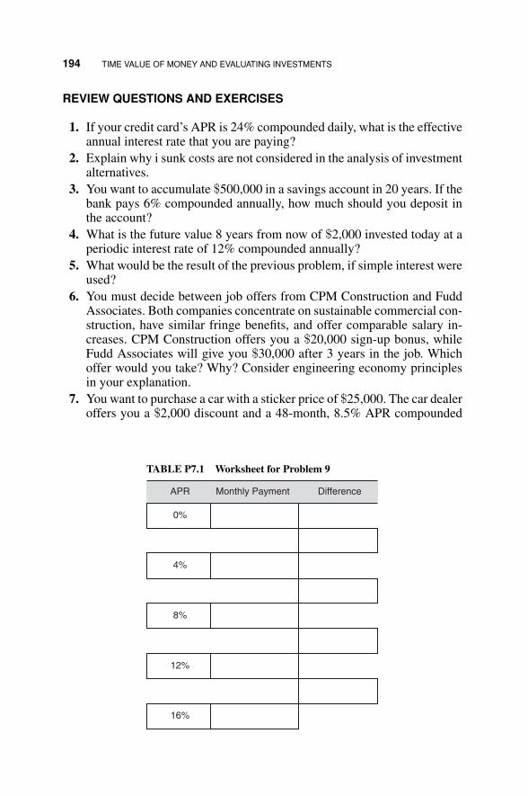
P1: OTA/XYZ P2: ABC




1. If your credit card’s APR is 24% compounded daily, what is the effectiveannual interest rate that you are paying?

2. Explain why i sunk costs are not considered in the analysis of investmentalternatives.

3. You want to accumulate $500,000 in a savings account in 20 years. If thebank pays 6% compounded annually, how much should you deposit inthe account?

4. What is the future value 8 years from now of $2,000 invested today at aperiodic interest rate of 12% compounded annually?

5. What would be the result of the previous problem, if simple interest wereused?

6. You must decide between job offers from CPM Construction and FuddAssociates. Both companies concentrate on sustainable commercial con-struction, have similar fringe benefits, and offer comparable salary in-creases. CPM Construction offers you a $20,000 sign-up bonus, whileFudd Associates will give you $30,000 after 3 years in the job. Whichoffer would you take? Why? Consider engineering economy principlesin your explanation.

7. You want to purchase a car with a sticker price of $25,000. The car dealeroffers you a $2,000 discount and a 48-month, 8.5% APR compounded

TABLE P7.1 Worksheet for Problem 9

APR Monthly Payment Difference

0%

4%

8%

12%

16%

P1: OTA/XYZ P2: ABC




A B C D E

APR

MonthlyPayment

(From previousproblem)

Totalpayment(1.15 ×

Column B)

AnnualPayment

(12 ×Column C)

MinimumAnnualIncome

(Column D / 12)

0%

4%

8%

12%

16%

monthly, or no discount with a 4.0% APR on a 48-month loan. Whichoffer is better?

8. Repeat the preceding problem, considering an inflation of 4.0%. Howdoes inflation affect the results of the previous problem?

9. Develop Table P7.1 comparing the monthly payments for a 30-year$200,000 mortgage loan with its APR compounded monthly.

10. The total monthly payment for a home mortgage loan is affected by theproperty tax and insurance. This amount is around 15% of the principalplus interest payment that you calculated in the previous problem. More-over, as a rule of thumb, a family should not devote more than 28% ofits gross income for home loan payments. With this information, find theamount that a family must earn to afford a $200,000 mortgage loan usingthe APRs of the previous problem. Table P7.2 should help you in yourcomputations.

11. Develop Table P7.3 comparing the monthly payments for a $200,000mortgage loan with an 8.00% APR compounded monthly.

12. Find the minimum amount that a family should earn to afford the mort-gage loan in the preceding loan scenarios. Use the same assumptions ofthe previous similar problem, and Table P7.4.

13. CPM Construction plans to buy a truck for $150,000 and sell it for$15,000 at the end of five years. The annual operating cost of the vehicleis $60,000. What is the equivalent annual cost of this truck, if the companyuses a MARR of 12%?

14. What is the present value of the truck described in Question 13?15. CPM Construction plans to charge $100,000/year for the truck de-

scribed in Question 13 (since the annual operating cost is estimated

P1: OTA/XYZ P2: ABC




100

30

15

10

5

Years Monthly Payment Difference


A B C D E

Years

MonthlyPayment

(From previousproblem)

Totalpayment(1.15 ×

Column B)

AnnualPayment

(12 ×Column C)

MinimumAnnualIncome

(Column D / 12)

100

30

15

10

5

at $60,000, this means that the annual income will be $40,000). What isthe IRR of this investment? Given CPM’s MARR, is this an attractiveinvestment?

16. Suppose that for the multipurpose sports stadium example consideredin the Owner Financing Using Bonds section, the bond issue was

P1: OTA/XYZ P2: ABC



40 years and the annual interest rate is 9% of the bond principal. Us-ing the architect’s estimate of cost of $41 million, determine the effectiveinterest rate.

17. Suppose in the preceding problem that the bonds are financed by a bankthat discounts the bond issue to $40 million. What is the new effectiveinterest rate?

P1: OTA/XYZ P2: ABC


CHAPTER 8

CONSTRUCTION LOANS AND CREDIT

INTRODUCTION

The ability to borrow or access funds plays a critical role in the constructionindustry. Construction loans and credit can be thought of as the air that inflatesthe balloon we call the economy. Without it, the economy shrinks, businessdries up and projects shut down. This chapter addresses the subject of creditand borrowing and how they provide the monetary flexibility to keep theindustry moving forward.

As has been emphasized in Chapter 1 and throughout this text, construc-tion is a project-based industry. This strongly influences how construction isfinanced. Construction financing is mainly concerned with (1) project financ-ing and (2) company financing. Project financing is effectively a short-termactivity tied to “line of credit” issues and protocols. Short-term financing, asthe name indicates, has to do with loans or credit, which must be repaid inthe “near future.” This can be defined as anywhere from a week to a year,depending upon stipulations established by the lender.

Company financing is handled mainly using commercial bank loans andretained earnings from within the firm or organization. This is in strong con-trast to other major industries in which development of capital for companyoperations and expansion is based upon the issuance of stock and the gen-eration of new funds from capital markets. Except in the in the very largestconstruction companies, generation of new capital by issuing stock is notthe norm. Most construction firms are small to medium-sized closely heldcompanies that attempt to avoid dilution of ownership by the issuance ofadditional stock.

199



P1: OTA/XYZ P2: ABC


200 CONSTRUCTION LOANS AND CREDIT

Therefore, development of new external capital for expanded operationscomes through borrowing from commercial banks in the form of long-termfinancing. Long-term financing refers to borrowing and loans that are to berepaid over a multiyear period. It is used for the acquisition of long-termassets such as equipment or real property.

Rising construction costs have increased the pressure on the industry tocarefully monitor costs and predict cash timing to better balance the flowof receipts and disbursements. To remain competitive, contractors are beingforced to manage liquidity by using new credit and borrowing strategies. Inthis chapter, development of external financing in the form of both short-termproject-oriented financing and long-term financing will be discussed. Thetopic of project development will be presented in order to become familiarwith some of the basic terminology and concepts associated with both short-and long-term financing. This will provide a basis for an in-depth discussionof credit and borrowing from the contractor’s perspective.

THE CONSTRUCTION FINANCING PROCESS

Money is often referred to as one of the 4 M’s of construction, the other threebeing manpower, machines, and material. It is a cascading resource that isencountered at various levels of project development. The owner or developermust have money available to initiate construction. The contractor (as yousaw in Chapter 6) must have cash reserves available to maintain continuityof operations since progress payments lag actual construction expenditures.The major agents involved in the flow of cash in the construction process areshown in simple schematic format in Figure 8.1.

The owner’s financing of any significant undertaking typically requires twotypes of credit: short-term financing during the development and constructionperiod and long-term financing during the operational life of the project. Theshort-term financing usually occurs in the form of a construction loan. Long-term financing involves a mortgage loan or similar funding scheme (e.g.,issuance of bonds, etc.) over an extended period of time (10, 15, 30, or moreyears).

Short-term loans may provide funds for items such as facility construction,land purchases, or land development. Typically, these short-term loans extendover the construction period of the project. A short-term loan is provided

Constructionlender

Owner/developer

Primecontractor

Subcontractor

$

Figure 8.1 Project money flow.

P1: OTA/XYZ P2: ABC


THE CONSTRUCTION FINANCING PROCESS 201

by a lending institution, based on the assurance that it will be repaid withinterest, by some other loan. This subsequent mortgage loan constitutes thelong-term financing. Therefore, the first objective of any entrepreneur is toseek a commitment for long-term, or permanent, financing from a mortgagelender. Regardless of the type of project, this commitment will permit theconstruction loan, and any other funding required to be obtained with relativeease or, at least, more easily.

Unless the development company is in a position to raise the funds requireddirectly by the issuance of their own securities (e.g. stock, bonds, etc.), it willseek to obtain a commitment from one of several alternate sources, includingreal estate investment trusts (REITs), investment or merchant banks, commer-cial banks, savings and loan associations, insurance companies, governmentalagencies (VA, FHA), or, in special cases, from one of the international devel-opment banks. Public institutions, and to an increasing extent private entities,are raising funds by the sale of bonds.

The choice of lender depends on the type and size of the project. Thechoice of the form of security employed depends on a number of factors suchas relative cost, the time period for which the funds will be available, thedegree of flexibility involved (e.g., the freedom to pay out or refinance) andwhether there are any restrictions involved which result in significant sacrificeof control to the lender. The funding of some larger projects may be handledby a consortium of international bankers (e.g., the English Channel Tunnel).

Notwithstanding recent developments in financial markets, lending insti-tutions tend to be cautious: They are not interested in financing failure or inowning partially completed projects. Therefore, they will undertake a greatdeal of research and evaluation prior to providing a commitment for funding.At a minimum, an entrepreneur will be expected to provide the informationgiven in Table 8.1.

In response to the recent financial crisis, many lending institutions are alsorequiring up to 75% of developmental projects to have lease agreements orcommitments from major occupants in place (i.e., to support the pro forma

TABLE 8.1 Business Plan Documentation

Documents included in a typical Business Plan1. Company financial statements2. Company principals financial statements3. Clear title to land involved in business proposal (if any)4. Zoning approvals (if appropriate)5. Preliminary architectural drawings (as appropriate)6. Preliminary cost estimates7. Preliminary implementation estimate8. Market Research9. Pro forma of expected income and expenses

P1: OTA/XYZ P2: ABC



Market rent for subject property (unfurnished) 55 two-bedroom A, B,or C units—1167 sq ft @ 41.0 cents/sq ft = $478.47/mo or $480 × 55 $26,400.00

20 three-bedroom A, B, units—1555 sq ft @ 37.3 cents/sq ft = $580.00/mo $580 × 20 11,600.00

Total estimated monthly income $38,000.00Other income: Coin laundry, vending machine 150.00

$38,150.00× 12 = annual total 457,800.00Less vacancy factor of 5% (based on historical data) −22,890.00Adjusted gross annual income 434,910.00Less estimated expenses @ 29.45% −128,080.00Net income before debt service $306,830.00

Capitalized value @ 9.5% = $3,229,789.00 =[

$306,830

(0.095)

]

Requested loan value = $2,422,000.00Loan/value ratio = 75% (high) governed by lowLong-term debt service @ 9.75% constant = $236,145.00Debt service coverage ratio = 1.3Loan per unit = $32,293.33Loan per square foot = $25.42

Figure 8.2 Pro forma for 75 apartment units.

of expected income and expenses) before entering into a long-term financialagreement. This, of course, reduces the speculative nature of the income flowassociated with the project. The concept of “Build it, and they will come” isa thing of the past.

A SAMPLE DEVELOPMENTAL PROJECT

Let’s consider a typical project. An example of a pro forma for a ventureinvolving the construction and leasing of a 75-unit apartment complex isshown in Figure 8.2. This document indicates that the annual income fromthe proposed apartment project will be $306,830. The requested loan is$2,422,000, and the annual debt service (i.e., interest) on this amount is$236,145, realizing an income after debt service of approximately $70,000.The ratio between income and debt service is 1.3. Lenders normally wishthis ratio to be below 1.3.

The basis for the loan amount is given in Figure 8.3. Items 1 to 34 areconstruction-related items and are developed from standard references (e.g.,R. S. Means, Co., Building and Construction Cost Data [published annually])based on measures such as square footage. The lender normally has a unit-price guide for use in verifying these figures. Items 35 to 46 in Figure 8.3cover non-construction costs that are incurred by the entrepreneur. It should

P1: OTA/XYZ P2: ABC


A SAMPLE DEVELOPMENTAL PROJECT 203

1.2.3.4.5.6.7.8.9.

10.11.12.13.14.15.16.17.18.19.20.21.22.23.24.25.26.27.28.29.30.31.32.33.34.35.36.37.38.39.40.41.42.43.44.45.46.

Construction-RalatedCosts

Non-ConstructionCosts

Total $2,422,000

Excavation and gradingStorm sewersSanitary sewersWater linesElectric linesFoundationsSlabsLumber and sheathingRough carpentryFinish carpentryRoofing and laborDrywall and plasterInsulationMillworkHardwarePlumbingHeating and air conditioningElectricalLinoleum and tileCarpetingKitchen cabinetsPainting and decoratingMasonry, blockMasonry, brickRanges and hoodsDisposalsExhaust fansRefrigeratorPavingWalks and curbsLandscapingFence and wallsFireplaceCleanupLender’s feeSurveyor’s feeArchitect’s feeLand costAttorney’s feeTitle insurance premiumOther closing costsHazard insurance premiumConstruction loan interestAppraisalBuilding permitTax

$ 67,50048,00084,03028,00014,00031,00096,000

185,000185,00081,36220,03570,00028,888

140,5568,813

165,00095,02590,35017,752

101,88162,075

107,00020,680

100,20029,6383,1391,022

35,04020,91520,79230,00036,79251,10029,20032,0001,000

12,50080,0007,5005,762

1504,780

120,000750

1,50050,000

Figure 8.3 Construction cost breakdown for 75 apartment units.

P1: OTA/XYZ P2: ABC



be noticed that the interest for the construction loan is included in the costscarried forward in the long-term financing.

The method used to calculate the actual dollar amount of the loan is of greatinterest to the developer. The interest paid for the use of the borrowed money isan expense, and it is generally considered prudent business policy to minimizeexpenses. One way to minimize the interest expense would be to borrow aslittle a possible. The developer is, however, interested in putting as little of hisown capital as possible at risk. Therefore, there is an incentive to use moniesprovided by others. This means borrowing as much as possible. That is, thedeveloper tries to expand his own small initial capital input to start the projectinto a large amount of usable capital provided by others. This is the principle ofleveraging. The entrepreneur takes a small amount and expands or leveragesit into a large amount. The more he invests, the more he stands to lose.

Prudent lending organizations are normally careful, however, to ensurethat the developer (i.e. the borrower in this case) has a sufficient amountof capital in the project so that if it fails, the developer’s losses will besignificant. This is the motivation for the borrower to push the project forwardto a successful and profitable result. It is not prudent to allow the primemover for a project to assume that if the project fails, he or she can simplewalk away with minimum damage. There must to painful consequences forthe borrower in the event of a failure.

Lack of attention to this basic concept was one of many elements thatled to failure and worse during the so-called “subprime” financial crisisof 2008. Loans were made with no down payment and very little or noneof the borrower’s capital at risk. In addition, many borrowers were notproperly vetted and were not able to pay the terms of the loan. The borrowersdefaulted (i.e., failed to make repayment) and lenders were confronted withthe ownership of assets that could not cover the amount of the borrowing.

THE AMOUNT OF THE LOAN

The amount of the mortgage loan should be a happy medium between toomuch and too little. If the loan is too small, there will not be enough tocover the costs of the project. On the other hand, if the loan is too large, thedeveloper will find that the individual loan payments will exceed the availablerevenue, and he or she may be unable to meet their obligations.

The amount the lender is willing to lend is derived from two concepts:the economic value of the project and the capitalization rate (cap rate). Theeconomic value of the project is a measure of the project’s ability to earnmoney. One method of predicting the economic value is called the incomeapproach to value and is the method shown in Figure 8.2. Simply stated, itis the result of an estimated income statement of the project in operation.Like any income statement, it shows the various types of revenue and theirsum. These are matched against the predicted sums of the different expenses.

P1: OTA/XYZ P2: ABC


HOW IS THE CAP RATE DETERMINED? 205

Although the predicted net income is a function of many estimated numbers,commonly, a fairly reasonable degree of accuracy is achieved. The expectednet income divided by the cap rate produces the economic value of the project.The cap rate used in this example is 9.5%. The capitalized economic value ofthe project is obtained by dividing the net income ($306,830) by the cap ratefactor (0.095). This yields an economic value of $3,229,789.

HOW IS THE CAP RATE DETERMINED?

Of course, the critical factor in the determination of the economic value isthe cap rate. This must be determined for the situation at hand. First, thelender generally provides a loan that is about 75% of the estimated economicvalue of the project. This is done because 25% of the value, or thereabouts,must be invested by the developer to serve as an incentive for making theproject a success. That is, a prudent lender furnishes 75% and the developerfurnishes 25%. The lender must then decide what the interest rate will beand considers what will be the developer’s rate of return. The sum of thesenumbers, times their respective portions, gives the cap rate.

Assume that the lender decides that an appropriate interest rate, givenmarket conditions, will be 8.5% and the developer’s planned rate of returnwill be 12%. Then the cap rate is taken as the weighted average of these twovalues. It is calculated as 8.5% times 75% plus 12% times 25%, which yields9.375% or 0.09375 as the cap rate factor. Obviously, the value of the caprate can be adjusted by the values that the lender places on his interest andthe developer’s rate of return. These numbers are a function of the existingeconomic conditions and thus fluctuate with the state of the economy. Thelender, therefore, cannot exert as much influence on their values as might atfirst be expected. The lender is not in the business of pricing himself out ofthe lending market. He will attempt to establish a rate that is conservative(from the point of security of the loan) but attractive. The expected incomedivided by the cap rate gives us the economic value. The loan value may thenbe on the order of 75% of the calculated economic value.

Not every lender, however, will follow this formulaic type of approach.Some lenders may have a policy of lending a fixed proportion of what theyview as the assessed valuation, which may not be based on the economicvalue. The assessment will be made upon the actual market value of theproperty as opposed to the potential economic value. This is the approachused for home and single-family residential mortgage loans.

The long-term financing for a project is critical. For this reason, the com-pany or individual developing the project may exercise the right to hire aprofessional mortgage broker whose business is to find a source of fundsand service mortgage loan activities. The broker’s reputation is based on theability to obtain the correct size mortgage loan at the best rate that is alsofair to his client. The broker acts as an advisor to the client, keeping him or

P1: OTA/XYZ P2: ABC



her apprised of all details of the proposed financing in advance of actuallyentering into the commitment. For this service, the mortgage loan brokerreceives a fee of about 2% of the loan, although the rate and amount will varywith the size of the loan.

MORTGAGE LOAN COMMITMENT

Once the lending institution has reviewed the venture and the loan committeehas approved the loan, a preliminary commitment is issued. Most institu-tions reserve their final commitment approval until they have reviewed andapproved the final construction plans and specifications.

The commitment issued is later embodied in a formal contract betweenthe lender and borrower, with the borrower pledging to construct the projectfollowing the approved plans, and the lender agreeing that upon constructioncompletion, and the achievement of target occupancy, he will provide thefunds agreed upon at the stated interest rate for the stated period of time. Asnoted earlier, the actual amount of funds provided generally is less than theentire amount needed for the venture. This difference, called owner’s equity,must be furnished from the entrepreneur’s own funds or from some othersource. The formal commitment will define the floor and ceiling amounts ofthe long-term loan.

During the construction period, no money flows from the long-term lenderto the borrower. Funds necessary for construction must be provided by theentrepreneur or obtained from a short-term construction lender. Typically, thelender of the long-term will pay off the short-term loan in full, at the time ofconstruction completion, thereby canceling the construction loan and leavingthe borrower with a long-term debt to the mortgage lender.

CONSTRUCTION LOAN

Once the long-term financing commitment has been obtained, the negotiationof a construction loan is possible. Very often commercial banks make con-struction loans because they have some guarantee in knowing the loan willbe repaid from the long-term financing. However, even in these situations,there are definite risks involved for the short-term lender. These risks relate tothe possibility that the entrepreneur or contractor may, during construction,find themselves in financial difficulties. If this occurs, it may not be possiblefor the entrepreneur/contractor to complete the project, in which case theconstruction lender may have to take over the job and initiate action for itscompletion. This risk is offset by a discount (1–2%), which is deducted fromthe loan before any money is disbursed. For example, if the amount of con-struction money desired is $1,000,000, the borrower signs a note that he willpay back $1,020.000. The borrower, in effect, pays immediately an interestof $20,000. This is referred to as a discount and may be viewed as an addi-tional interest rate for the construction loan. The current trend to minimize

P1: OTA/XYZ P2: ABC


CONSTRUCTION LOAN 207

these risks is to require the borrower to designate his intended contractor anddesign architect. The lender may also require that all contactors involved inthe construction be bonded as well. Some commercial banks evaluate andseek to approve the owner’s intended contractor, his prime subcontractors,and the owner’s architect, as a prerequisite to approving the construction loan.This evaluation extends to an evaluation of their financial positions, technicalcapabilities, and current workloads.

To minimize the risks involved, the banks will also base their constructionloans on the floor of the mortgage loan, and only 75 to 80% of this floorwill be lent. Of course, the developer may need additional funds to coverconstruction costs. One way to ensure this is to finance the gap betweenthe floor and ceiling of the long-term mortgage loan. The entrepreneurgoes to a lender specializing in this type of financing and obtains a standbycommitment to cover the difference or gap between what the long-termlender provides and the ceiling of the long-term mortgage. Then, if theentrepreneur fails to achieve the breakeven rent roll or similar requirement,he still is ensured of the ceiling amount. In this situation, the constructionlender will provide 75 to 80% of the ceiling rather than the floor. If thefloor of the loan is $2,700,000 and the ceiling is $3,000,000, the financingof the gap can lead to an additional $240,000 for construction (i.e., 80% of$300,000). Financing of the gap is usually expensive, requiring a prepaidamount of as much as 5% to the gap lender. In the preceding example, thiswould be $15,000 paid for money that may not be required if the rent roll isachieved. Nevertheless, the additional $240,000 of construction funding maybe critical to completion of the project and, therefore, the $15,000 is wellspent in ensuring that the construction loan will include this gap funding.

Once the construction loan has been approved, the lender sets up a drawschedule for the builder or contractor. This draw schedule allows the releaseof funds in a defined pattern, depending on the site and length of the project.Smaller projects, such as single-unit residential housing, will be set up forpartial payments based on completion of various stages of construction (i.e.,foundation. framing, roofing, and interior), corresponding to the work of thevarious subcontractors who must be paid. For larger projects, the draw sched-ule is based on monthly payments. The contractor will invoice the owner eachmonth for the work he has put in place that month. This request for funds isusually sent to the owner’s representative or architect, who certifies the quan-tities and value of work in place. Once approved by the architect and represen-tative, the bank will issue payment for the invoice, less an owner’s retainage.

The owner’s retainage is a provision written into the contract as an incentivefor the contractor to continue his efforts, as well as a reserve fund to coverdefective work that must be made good by the contractor before the retainageis released. Typically, this retainage is 10%, although various decreasingformulas are also used. When the project is completed, approved, cleared,and taken over by the owner, retainage is released to the builder.

In addition to the funds mentioned, the developer should be aware thatsome front money is usually required. These funds are needed to make a

P1: OTA/XYZ P2: ABC



good-faith deposit on the loan to cover architectural, legal, and surveyingfees and for the typical closing costs.

COMMERCIAL LENDERS

As noted in the Introduction to this Chapter commercial banks are the primarysource of loans for the construction industry. Banks normally have a loanoversight group, which reviews loan applications. Despite recent develop-ments in the credit and loan markets, bankers are typically conservative andstudy the financial position of potential borrowers very carefully. As notedabove, both personal and company financial statements are key documentsthat are reviewed to establish the credit worthiness of potential borrowers.The supporting documentation required is similar to that required shown inTable 8.1.

Lending organizations analyze the so-called “Three Cs” of lending:credit, capacity, and collateral when considering loans to various individuals,companies and other organizations (i.e., the local church planning to borrowto expand facilities, etc.). Credit refers to the borrower’s history of loanrepayment. Capacity considers the borrower’s ability to repay the loan giventhe borrower’s financial situation both in terms of income and expenses.Collateral refers to the value and quality of the assets that the borrower offersto secure a loan in the event it is not repaid. These are relatively quantitativemeasures, which provide a good basis for evaluating the potential of a givenborrower to repay the loan. During the recent financial crisis, it became ap-parent that these measures were subject to manipulation and a lack of clarity(i.e., transparency), which very nearly led to the shutdown of the nationaland international credit markets.

As noted in Chapter 6, retailers typically borrow money to purchase newinventory. As the inventory is sold, the revenue generated is used to retire theloan. Farmers borrow money to purchase the seed and equipment required toplant a crop or raise livestock. When revenues are generated through the saleof crops or livestock, the debt is retired and any profit is retained. If there is afear that borrowers will not be able to repay the loan, the credit markets canbe severely impacted. This occurred during the 2008 crisis to the degree thateven banks were reluctant to lend to each other because of the fear that theborrowing bank might be on shaky ground.

In addition to the three Cs noted above, two additional and more judgment-based (i.e., less quantitative) measures are often used by lending institutionsto evaluate potential borrowers. These relate to a qualitative evaluation ofa potential borrower’s credit worthiness. These two Cs are character andcapital. Character refers to the financial reputation of the borrower and tomore subtle qualities such as trustworthiness and issues related to reliabilityand reputation. Capital considers the borrower’s total volume of and accessto assets.

P1: OTA/XYZ P2: ABC


LINES OF CREDIT 209

The actual process of applying for a loan, line of credit, or a credit account,although based on the preceding principles, is much more specific. Tax returns,credit ratings, job information, and detailed personal data are required in apersonal loan application. A loan application for a real estate developmentproject requires a business plan explaining the income projections that thedeveloper anticipates will be used to repay the loan. There are many sources ofinformation for positive and negative factors that must be taken into accountby the bank when evaluating such loan applications.

LINES OF CREDIT

A line of credit is an arrangement for loosely secured credit up to a certainamount and operates in a manner similar to a personal credit card. This is aso-called “revolving” type of credit. This means that monies are withdrawnand repaid on a continuous basis over the period of the loan. The short-termfinancing used by contractors to carry the costs of a project over the periodof a project is an obvious example of a line of credit loan. Interest is paidon the outstanding balance, with a smaller fee paid on the unused portion ofthe credit as discussed below. Payments can be variable, subject to conditionsdiscussed in this section. Again as with a credit card, the borrower charges“purchases,” which can include a wide variety of liabilities such as payroll,material purchases, and business related expenses.

On the other hand, the Maturity Matching Principle is a protocol thatprecludes the purchase of major assets such as a piece of heavy equipmentor a major home office computer system using a line of credit. This protocoldictates that line of credit and similar short-term financing should be usedto realize short-term and clearly defined business activities (e.g., inventoryfinancing, crop planting, contractor project financing, etc.). As discussed inthe Introduction to this chapter, the intent is that the loan will be repaid over ashort term, (e.g., months as opposed to years). In other words, buying a houseor a private airplane using a credit card is not acceptable. Major purchases ofequipment and real property and similar long-term assets require the use oflong-term financing.

The credit card analogy is useful for explanation purposes, but it must benoted that there are significant differences between a personal credit card andshort-term financing using a line of credit. Major differences have to do withthe following:

1. Interest paid on outstanding balances2. Commitment fees paid3. Maintenance of outstanding balances4. Clean-up requirements5. Collateral required

P1: OTA/XYZ P2: ABC



INTEREST PAID ON OUTSTANDING BALANCE

The interest accrued on a line of credit is computed by multiplying the balanceby the agreed-upon interest rate. An APR of, say, 12% will result in charginga daily interest rate of 12%/365. This daily interest rate is then multipliedby the balance that the account had each day of the month. The monthlystatement will be equal to the outstanding balance at the end of the month,plus all interest accrued for the days in the month.

Example: A line of credit has a balance of $500,000 during the first15 days of July, and $400,000 during the remaining 16 days. If the agreedupon APR is 12% compounded daily, what is the total interest for the month?

Answer: the first day of the month accrues an interest of $500,000 ×(0.12/365) = $164.38. The second day accrues interest on $500,000 +$164.38, or $500,164.38 × (0.12/365) = $164.44. The third day will have toconsider ($500,000 + $164.38 + $164.44) = $500,328.82. The computationfor the 31 days are summarized in Table 8.2. The total interest for the monthis $4,626.81 for a payable balance of $404,626.81.

This total is very close to the one resulting from multiplying the account’saverage for the month by APR/12. That is:

Average for the month = ($500,000 × 15 + $400,000 × 16)/31

= $448,387.10

Interest for the month = $448,387.10 × (12%/12) = $4483.87

Virtually all banks compute interest using the average daily balance, sothis monthly amount would be technically incorrect.

TABLE 8.2 Interest Computations for Outstanding Balance

Day Principal Added Interest Cumulative Interest New Principal + Interest

1 500,000.00 164.38 164.38 500,164.382 500,000.00 164.44 328.82 500,328.823 500,000.00 164.49 493.31 500,493.314 500,000.00 164.55 657.86 500,657.865 500,000.00 164.60 822.46 500,822.46

. . .

15 500,000.00 165.14 2,471.44 502,471.4416 400,000.00 165.20 2,636.63 402,636.63. . .

30 400,000.00 132.94 4,493.83 404,493.8331 400,000.00 132.98 4,626.81 404,626.81

P1: OTA/XYZ P2: ABC


COMPENSATING BALNCES 211

COMMITMENT FEES

This requirement, as well as others discussed in the following sections, under-line the differences between lines of credit from credit cards. Lenders imposea commitment fee on the unused portion of the line of credit. This fee usuallyhas an APR of between 1/2% and 1%, although it varies with the market andthe client’s credit credentials (large clients with excellent credit may evenhave this fee waived).

Example: A line of credit has a limit of $1,000,000 and had an average of$400,000 for July. How much is the commitment fee for the month, if it hasan APR of 1% compounded daily?

Answer: The formula to find the amount, which is derived from topicsdiscussed in Chapter 8, is:

Fee = P × (1 + i)n − P, where

P = $1,000,000 − $400,000 = $600,000;

i = 1%/365, and n = 31 days

Fee = [600,000 × (1 + 0.01/365)31] − $600,000 = $509.80

This fee raises the effective interest paid on a line of credit. If a line ofcredit maintains a balance of 50% of its limit and has a commitment fee of1%, the added annual effect on the effective interest paid would be computedas: i′ = 50% × (1+ 0.01/365) 365 – 50% = 0.5025%

COMPENSATING BALANCES

A line of credit may require that the borrower keeps an account in the samelending institution with a minimum balance of a given percentage of thecredit limit. This percentage varies depending on the credit worthiness ofthe borrower and the lender policy. A 10% minimum is a common figure.The account can be interest bearing or non-interest-bearing, although lendersincreasingly allow only non-interest-bearing accounts.

A compensating balance is a form of collateralization. It guarantees thatthe borrower will have at least some funds under the lending institution’scontrol to pay any outstanding balance. From the borrower’s perspective, itis an undesirable requirement. If the compensating balance is 10%, it meansthat the actual money contributed by the line of credit is, in fact, 90% of itsstated limit.

The first 10% of the outstanding balance at any given time would be simplyoffsetting the unmovable money sitting in the account as a compensatingbalance. A compensating balance increases the effective interest paid by theborrower.

P1: OTA/XYZ P2: ABC



Consider the case of a contractor needing $400,000 to cover the peak of thefluctuations in his cash flow. Suppose that these fluctuations average $200,000.Assume that he wants to have an extra $100,000 as a cushion for emergencies.If a 10% compensating balance in a non-interest-bearing account is stipulatedby the lender, it means that instead of the $400,000 + $100,000 = $500,000that the contractor actually intends to use, he will have to ask for $555,000,so that the frozen 10% (approximately $55,000) does not hinder its cashavailability. The average balance for the line of credit will be $255,000 insteadof $200,000. This is $255K/$200K = 1.275 or 27.5% more than the intendedaverage. If the line of credit has an APR of 12%, the contractor will end uppaying, on the average, an APR of 12% × 1.275 = 15.3%.

CLEAN-UP REQUIREMENT

Most lines of credit are required to be paid in full and remain with a balance ofzero for a number of consecutive days each year. This clean-up requirementis an elegant way of forcing the borrower to keep in mind that a line of creditis a short-term loan arrangement, not a long-term one. There are severalgood reasons to separate these two categories of loans, from the lender’sperspective. An important reason is that lines of credit and long-term loansrequire different collaterals, and therefore, the lender is exposed to differentrisk levels. When a line of credit does not contain a clean-up requirement, itis known in the lending trade as an evergreen loan.

COLLATERALS

A line of credit is considered to be a loosely secured financial arrange-ment. The assets that are offered as a guarantee for its repayment are calledcollateral. For lines of credit, collateral requirements are not a stringent as inthe case of long-term loans. In many cases, a borrower can show that his orher financial strength is sufficient to allow clean up of the line of credit with-out materially impacting the borrower’s financial position. In some cases,the lender may establish additional requirements involving supplementarycollateral.

A common requirement requires that a second party endorse the terms ofthe loan, in effect agreeing to repay the loan in the event that the borrowerdefaults on payment. This person or entity is referred to as a cosigner. Thecosigner agrees to repay the interest and borrowed amount of the loan in theevent that the primary borrower defaults.

An alternative to cosigning is to pledge a specific asset as collateral. If theasset is real estate, a mortgage can be filed benefiting the lender. A mortgage

P1: OTA/XYZ P2: ABC


TRADE CREDITS 213

is a specific form of lien against a property, which will be voided when theloan is paid, or executed in foreclosure if the borrower fails to follow theloan agreement. Despite the common misuse of the word, a mortgage is nota loan. It is a claim allowing foreclosure on the subject property in the eventof default by the borrower.

ACCOUNTS RECEIVABLE FINANCING

In very unusual cases, contractors experiencing an urgent cash flow problemcan use accounts receivable as collateral. A lender may accept accounts re-ceivable as collateral in special situations. This arrangement is called accountsreceivable pledging. Since this type of collateral presents a higher level ofrisk (Can collection of the accounts receivable, in fact, be made?), the lenderwill charge a high interest for such loans. The maximum amount of the loandepends on the amount and age of the accounts receivable.

A lender may agree to provide funds up to 75% of the value of accountsreceivable due between 0 and 30 days. Older outstanding balances usuallyindicate that the account may be difficult to collect. The lender would viewthese accounts as being of higher risk and might lend up to 60% of the balanceof accounts aged between 31 and 60 days.

In extreme financial emergencies, a firm may even sell its accounts re-ceivable at a discount. This method of raising funds is called factoring. Asdiscussed previously, the discount depends on the age of the accounts. Fundsgenerated from factoring are not a loan, but a final transfer of funds to thebuying agency. Clearly, this is a risky business for both seller and purchaser,and is seldom utilized by construction firms.

One advantage accruing to the seller is that responsibility for collectionof the accounts is transferred to the purchasing entity—the factor. Justthe cost of collecting money from slow or delinquent clients may justifythe use of factoring. It is a quick way to obtain cash, and does not require theadministrative burden of seeking a bank loan.

TRADE CREDITS

Trade credits are, in effect, free money provided to a company by its suppliers.It has a significant effect on a construction contractor’s cash flow. Suppliersand subcontractors extend credit to contractors to encourage quick and timelypayment. From the vendor’s perspective, incentives for timely payment leadto a reduction in the carrying costs associated with inventory financing.

Suppliers have clearly defined credit terms, including the number of daysallowed for payment before interest or fees apply and discounts for earlypayment. The typical credit account will stipulate 30, 60, or even 90 calendar

P1: OTA/XYZ P2: ABC



days for payment, although in some cases credit can be for as few as 10 oreven 7 days. It is important to verify whether credit terms are specified incalendar days, which is the most common case, or in business days. Lack oftimely payment can lead to a negative reading of the financial “character” ofthe purchaser on behalf of creditors.

The leverage provided by trade credit on the availability of cash can dra-matically improve the viability of any company. These considerations under-score the importance of having a pristine payment record with all merchantsextending credit to a company. An impeccable record serves as the bestbusiness card to get further credit with other lenders. It also is the best argu-ment to get an extension of payment terms or to increase the limit of creditwhen needed. Simply stated, timely payment leads to an excellent “creditrating.”

Credit arrangements with subcontractors tend to be less stringent than thoseafforded by commercial suppliers. All subcontractors want to be consideredfor future jobs by the contractor, and seldom stipulate credit terms such asthose discussed above. Subcontractors are also inclined to accept subcontractsthat include “pay when paid” clauses. With such clauses, the subcontractorextends credit to the prime contractor for an indefinite period until the projectowner supplies the funds to pay the subcontractor.

Vendors and suppliers deal with many customers and are much more de-manding in encouraging and requiring timely payment. Invoices from vendorstypically include compact information about payment terms, such as “2/10,net 30.” The “net 30” means that the merchant expects that the invoice willbe paid in full by the 30th calendar day after the date printed in the invoice.The “2/10” indicates that if payment is made within 10 calendar days, a 2%discount will be applied.

For an invoice totaling $1,000, this yields a $20 discount. This amountmay seem insignificant, and a fair proportion of contractors simply do nottake advantage of the offer. This is a great mistake. The annualized interestfor early payment can be computed as:

Effective annualized discount rate = (365/(30 − grace period))

×[Discount%/(100% − Discount%)]

For “2/10, net 30,” using the above formula, the discount rate is:

Effective annualized discount rate = (365/(30 − 10)) × (2%/(100% − 2%))

= 37.24%

This represents a 37.24% recovery on the average outstanding balance ofinvoices from vendors offering this discount.

P1: OTA/XYZ P2: ABC


LONG TERM FINANCING 215

Terminology relating to trade discounts is as follows:

ROG/AOG: The discount period begins upon receipt of goods (ROG)

2/10 NET 30 ROG: This expression appearing on the invoice means 2% can be deductedfrom the invoiced amount if the contractor pays within 10 days ofthe arrival or receipt of goods. Full payment is due within 30 daysof AOG/ROG.

2/10 PROX NET 30: A 2% cash discount is available if invoice is paid not later than the10th of the month following ROG. Payment is due in full by theend of the following month.

2/10 E.O.M.: The discount (2%) is available to the 11th of the month followingROG. Payment in full is due thereafter.

It is a longstanding “rule of thumb” in the construction industry that pay-ments to vendors offering discounts should always be made in a timely fashionto take advantage of such trade credits.

LONG TERM FINANCING

Banks and other financial institutions can provide term loans. A term loanmust be repaid by a given date, called its maturity date, and is repaid under aprearranged schedule. Although technically a term loan can be classified asa short-term loan if it is repaid within a year, such loans are primarily usedfor long-term financing. The term can be up to 15 years in most cases andeven more in noncommercial settings. The 30-year loan that many peopletake to finance their homes is a term loan, albeit more regulated than normalcommercial loans.

Term loans require an application process which, as noted previously,is usually quite elaborate. The prearranged timetable established for repay-ment of a term loan is called an amortization schedule. Most lenders requireequal monthly payments throughout the life of the loan, although there areexceptions.1

The equal payments to amortize a term loan are computed as an annuity(paid every month, despite the name suggesting yearly payment). For illus-tration purposes, and using formulas discussed in Chapter 7, it can be shownthat a $200,000 loan to be repaid in 30 years at a 7.00% APR compoundedmonthly results in 360 payments of $1,330.60. The same loan paid over15 years would have payments of 1,797.66. The difference in payments isrelatively small (35.1%), considering that the payment time is halved for the15 year option. The reason for this seemingly illogical proportion can be found

1 Production Credit Associations allow the payment of principal in equal amounts, with varying interestdepending on the remaining principal owed at any given time.

P1: OTA/XYZ P2: ABC



in the interest paid, which grows at a much faster rate than the repaymentperiod.

A term loan normally has fees that must be paid up front or deducted fromits principal. Some of these fees are quite justifiable, but others may strike theborrower as subject to negotiation. There are loan origination fees, application,credit investigation fees, and closing fees, among others. Higher fees areexpressed in points. Each point is 1% of the stated principal and, therefore,increases the nominal amount of the loan. In the case of the $200,000 loanat 30 years and APR of 7%, a 2-point fee translates into an extra $4,000,which usually is paid by increasing the nominal amount borrowed. Instead of$200,000, the loan would be for $204,000, with payments of $1,357.22. Over360 payments, the extra $26.62 per month turns into $9,582.15.

Construction contractors, as noted previously, do not need long-termfinancing except for the purchase of equipment, which normally leads toloans of no longer than 5 years. If the purchase of real property is part ofa company’s long-term planning, term loans of 15 to 30 years may be ofinterest. In general, however, long-term financing is limited to equipment andsimilar purchases.

LOANS WITH END-OF-TERM BALLOON PAYMENTS

When purchasing an item on credit, a contractor may choose to pay a highertotal loan interest if the terms of the load make the monthly installments moreaffordable during the first few years of loan repayment. That is the case whena contractor has a limited amount of cash to execute a project and needs topurchase a piece of equipment for the project. Instead of paying large monthlyinstallments, it may be advantageous to pay a smaller monthly amount duringthe project execution and then, at the end of a relatively short period, pay alarge lump sum to liquidate the loan principal that has not been repaid by thesmaller installments. The unpaid principal at the end of the period is calledthe balloon payment amount and the type of loan that allows this arrangementis called a loan with an end-of-term balloon payment. The following exampleillustrates how this type of borrowing might be implemented.

A heavy construction company plans to purchase a front loader. The initialcost of the loader is $80,000. The company desires to borrow $90,000 topay for taxes and other costs associated with the purchase. The bank offersa 9.00% APR and the loan must be repaid in no more than 5 years. Thecontractor wants to consider a balloon payment scheme to repay the loan.

First we will consider this purchase using a loan that stipulates uniformmonthly payments at 9.00% APR over the 5-year term of the loan. This willbe called Option A.

A second payment scheme will be called Option B. This payment sequenceuses a balloon payment to reduce the monthly payments over the 5 year(60 month) period of the loan. In this case, the amount of monthly payments

P1: OTA/XYZ P2: ABC


LOANS WITH END-OF-TERM BALLOON PAYMENTS 217

TABLE 8.3 Fully Amortized and Balloon Payment Loans

A) Fully amortized loanAmount borrowed $90,000APR (Compounded monthly) 9.00%Years for payment computations 5Monthly payments $1,868.25Payment due at the end of 5 years 0

B) Loan with balloon payment after 5 years,amortized on a 20 year scheduleAmount borrowed $90,000APR (Compounded monthly) 9.00%Years for payment computations 20Monthly payments $809.75Payment due at the end of 5 years $79,836.34

is based on uniform payments over a 20 year (240 month) term. However,the loan must be paid in full after 5 years. Therefore, at the end of 5 years,the remaining 15 years of the 20 year term will be paid out as a lump sum orballoon payment.

These two options (A & B), to include the monthly amounts and balloonpayment to be paid are summarized in Table 8.3.

The calculation of uniform payments for Option A simply requires theapplication on the formula A = $90,000 × (A/P, 0.75%, 60). This results inmonthly payments of $1,868.25.

The B Option involves reduced monthly payments (due to the 20 year term).The monthly payments are calculated as A = $90,000 × (A/P, 0.75%, 240).The 240 month period leads to a reduced monthly payment of $809.75. But,of course, the balloon payment must be paid at the end of the fifth year.

Therefore, we must calculate the present value of the remaining 15 yearsof payments comprising the balloon payment to be paid at the end of the fifthyear. This involves taking the 15 years of monthly payments to a single PWvalue to be paid at the end of year 5. P = $809.75 × (P/A, 0.75%, 180).N is 180 since there are 12 payments each year for 15 years (i.e.12 × 15) tobe considered. This yields a balloon payment of $79,836.34.

It can be observed that the balloon payment scheme results in paymentsof less than half of the uniform payments of Option A—$809.75 versus$1,868.25. The amount of the balloon payment is very large. After thefive years, the company would owe nothing under the fully amortized plan(Option A), while $79,836.34 would be still owed as a balloon payment underthe alternative payment scheme (Option B).

The total payment using Option A is 60 months times $1,868.25 or$112,095. The total pay out for Option B is 60 months times $809.75 plusthe balloon payment of $79,836.34. This amounts to $128,421.34. Reducing

P1: OTA/XYZ P2: ABC



the monthly payment and using a balloon payment will cost $16,326 morethan Option A. Under certain circumstances, this may be acceptable. Thecost versus the benefit must be carefully considered by the borrower. Lenderstend to be reluctant about such financing schemes due to the risk that theborrower may not be disciplined or reliable enough to escrow the requiredballoon payment. This where the Character—reliability and reputation—ofthe borrower must play a key role.


1. What does it mean when it is said that a company is “excessively lever-aged?” What could be the effects of excessive leverage? You may wantto search the phrase “effect of excessive leverage” on the Internet.

2. An entrepreneur is considering a new project consisting of an apartmentbuilding with 50 units. Each unit can be rented for $1,000/month. It isexpected to have an average vacancy rate of 10%. Net operating expensesare budgeted as 30% of the project’s gross annual income. What wouldbe the economic value of this project, using a cap rate of 8%?

3. How much would be the value of the long-term loan for the precedingproject? How would this amount change if the entrepreneur offers to puta $100 million hotel as collateral for the loan?

4. A line of credit has a balance of $700,000 during the first 10 days of June,and $300,000 during the remaining 20 days. If the agreed-upon APR is10% compounded daily, what is the total interest for the month?

5. A line of credit has a limit of $500,000 and had an average of $200,000for July. How much is the commitment fee for the month, if it has anAPR of 0.5% compounded daily?

6. Find the effective annualized discount rate offered by a supplier withpayment terms of “1/15, net 30.”

7. What is the monthly amortization of a 5-year term loan with a principalof $50,000 and an APR of 12% compounded monthly?

8. Find the monthly payment to amortize the balloon payment of $79,836.34remaining after 5 years for the example developed in Table 8.1. Assumethat the balloon amount must be repaid over 5 years, with an interest of9.00%.

9. Are construction contractors used as financing sources by project owners?What would be the terms of a “perfect” contract between a project ownerand a construction contractor, concerning financial resources?

10. Under what circumstances would you take the balloon payment schemediscussed in Table 8.3?

P1: OTA/XYZ P2: ABC


CHAPTER 9

THE IMPACT OF TAXES

INTRODUCTION

The profitability of any construction company is significantly affected by theamount of taxes it is required to pay. More than one third of a company’staxable income goes to pay its tax obligations to federal, state, and municipalentities. Understanding the rationale and conceptual framework of the currenttax system is, therefore, of paramount importance to any contractor. Financialchoices affect the amount of taxes paid and taxes affect the financial decisionsthat a construction company makes. This chapter provides an introductorytreatment to this topic. It must be kept in mind, however, that tax law changesconstantly and is continuously in a state of flux. Material presented in this textis based upon tax law and bulletins as of 2008. Keeping current on changesto this material is critical to managing the payment of tax obligations. TheInternal Revenue Service (IRS) website at www.irs.gov contains excellentreadable reference material that can help in keeping abreast of current eventsin this area. It is always, however, necessary to consult a tax expert beforemaking important decisions involving taxes.

Taxes are primarily designed to finance government operations and to meetsocietal needs. In modern societies, taxes have also been implemented toinfluence taxpayers’ behavior. For example, high taxes operate to increase theprice of tobacco, which presumably causes fewer individuals to use tobaccoproducts. Purchasing hybrid-powered cars results in significant tax creditsmeant to spur their use.

An unintended consequence of tax incentives and deterrents is that, oncethey are in place, they become extremely difficult to withdraw even whenthe issues that they originally addressed are no longer relevant. Obsolete tax

219



P1: OTA/XYZ P2: ABC


220 THE IMPACT OF TAXES

breaks still abound and are the focus of the activities of countless lobbyistsand politicians.

TYPES OF TAXES

A tax levied on the net income realized by a company or individual is calledan income tax. Income taxes are referred to as direct taxes. Indirect taxes, incontrast, are levied on the cost, price or value of products or services.1 TheU.S. government relied almost exclusively on taxing resources other thanincome until the Sixteenth Amendment to the Constitution was passed in1913 (previous attempts to impose income taxes were short-lived). Althoughthe focus of this chapter is on income taxes, everyone also pays indirect taxes.

Some forms of indirect taxes relate to:

1. Excise taxes. These taxes are levied on the output (not the price) of agood. Although historically significant, this tax is currently applied toa small number of products (e.g., gasoline.). The excise tax on gasolineis applied to each gallon, independently of its selling price.

2. Import and export taxes. These taxes (or duties) are imposed on mer-chandise arriving or leaving a country, respectively. These taxes arepopular in many countries with weak institutional administrative frame-works because they are easy to collect at their ports of entry and depar-ture. Import duties are frequently used for political leverage with theexporting country and to protect local industries from cheaper importedgoods.

3. Sales taxes. These taxes are computed as a percentage of the sellingprice of goods. In the United States, sales taxes are collected by mer-chants at the point of sale. In Europe, the Value Added Tax (VAT) isfunctionally similar from a consumer’s viewpoint, but the tax is col-lected progressively up the production and distribution chain of theproduct.

4. Ad valorem taxes. These taxes are levied on the estimated value of aproperty. The most common form of ad valorem tax is the propertytax imposed on real estate and its improvements. The semantics of theterm ad valorem has been used to argue that all taxes based on value(including sales and import/export) fall into this classification.

Most indirect taxes can be viewed as location-related in that they depend onthe area or location where the company or individual is based. This supports

1 Some legal scholars define indirect taxes as those collected by an intermediary from the person whoultimately pays the tax. This is the familiar case of the sales tax collected by a retail store and paid by thecustomer.

P1: OTA/XYZ P2: ABC


ALTERNATIVES FOR COMPANY LEGAL ORGANIZATION 221

the generation of local tax revenue and empowers citizens at the local level.Alternately, it can also result in a wide range of taxes that may put a brakeon economic activity. Because of this, certain states and municipalities areviewed as tax friendly, while others are not.

The U.S. government entrusts the Internal Revenue Service (IRS) with theadministration and collection of federal taxes. States and other levels of gov-ernment have their own tax collection agencies. Outside of the United States,most countries have agencies similar to the IRS to administer tax collection.Failure to pay taxes normally results in harsh penalties for tax evasion.

INCOME TAX SYSTEMS

Business entities pay tax on taxable income, which is the revenue earned by acompany minus the expense of doing business and any allowable deductions.Construction costs (direct costs plus field overhead) and general overheadcosts associated with the operation of a construction company are deductiblein principle, independent of the company’s form of business organization.However, some expenses are difficult to classify and others are not fullydeductible. For example, the IRS allows deduction of only half of the costincurred for business meals and entertainment.

Revenue minus all costs of generating said revenue is the definition ofprofit, and it is tempting to conclude that income taxes are applied to acompany’s profit. However, deductions authorized by tax law invariably leadto a company paying taxes on a lower amount than the amount of net profitreported to stake and/or stockholders. The net amount used to compute acompany’s tax liability is called its tax base or taxable income.

Tax deductions constitute major administrative tools for influencing tax-payers to consider and conform to what government authorities view as adesired behavior. Charitable contributions, solar energy generation systems,extra costs resulting from locating in certain inner cities and other reputedlydesirable deeds are rewarded by allowing costs associated with these actionsto be deducted from a company’s or individual’s revenue. Deductions are,however, the source of much of the complexity of the current income taxsystem.

ALTERNATIVES FOR COMPANY LEGAL ORGANIZATION

The legal form of organization adopted by a company influences many man-agement issues, including the level of effort required to start a company,minimum reporting requirements for its owners and government agencies,the risks faced by its owners in case of financial default, and the amountof taxes paid on its profits. This section offers a short summary of majororganizational forms, emphasizing their tax implications.

P1: OTA/XYZ P2: ABC



Sole Proprietorships

A company organized as a sole proprietorship has a single owner, who isultimately responsible for all its liabilities and enjoys all profit, if any, fromits operation. The company’s profit is treated as personal income for tax pur-poses. For instance, suppose that Elmer Fudd is the sole owner of Elmer FuddConstruction, a proprietorship whose profit was $500,000 for 2008. Addi-tionally, he had income of $10,000 from interest generated by his personalbank savings.

His total personal income would be $510,000. Assuming that he had noother sources of income, he is married filing jointly with no dependent chil-dren, and he chooses the standard IRS deduction, the amount of his federalincome tax for 2008 would be around $144,627. The details of this and thefollowing tax computations are discussed later in this section.

Partnerships

A partnership is similar to a proprietorship in that the owners are ultimatelyresponsible for all company liabilities and pay taxes on the profit receivedby each one. As in the case of proprietorships, a partnership is transparentfor taxation purposes. The company is not independently taxed, nor canit retain any proportion of its profits. Consequently, the account RetainedEarnings, discussed in the accounting chapters of this book, is meaninglessfor partnerships and proprietorships from a legal standpoint.

For comparison, suppose that Elmer Fudd and four nephews have equalownership rights in a partnership called Fudd and Nephews ConstructionCompany. The company had a profit of $500,000 for 2008. Each of the fivepartners is married filing jointly with no dependent children and received$2,000 in interest income. The total income of each one (their respectivegross adjusted income, as discussed later) would be $102,000. Each onewould pay approximately $13,713 of federal income tax, for a combined totalof $68,565. The difference between this figure and the tax paid by Mr. Fuddas a sole proprietor is quite significant.

Corporations

From a legal perspective, a corporation is considered a unique entity, separatefrom its owners. As such, the owners’ responsibility for its liabilities is limitedto their share of company equity. In contrast, a regular partner or a soleproprietor can lose virtually all personal property if it is necessary to payoff their company debts. The tradeoff of this substantial advantage is thatcorporation profits are taxed before any dividends are distributed to owners.Owners, in turn, must pay tax on the dividends they receive, albeit at a lowerrate than regular personal income. Most individuals paid a flat rate of 15%for dividends in 2008, as further discussed later.

P1: OTA/XYZ P2: ABC


ALTERNATIVES FOR COMPANY LEGAL ORGANIZATION 223

Suppose that Elmer Fudd and his four nephews decide to incorporate theircompany as Fudd Associates, Inc. The corporation earnings before incometaxes was $500,000 and all after-tax profit was distributed as dividends to thefive shareholders, each one receiving the same amount. Tax computations inthis case are more complicated than in the previous organizational forms.

The corporation would pay $170,000 in federal income taxes, and therefore,there would be $330,000 left over to distribute to owners. Each of the fiveowners would receive dividends of $66,000. The tax for this dividend amount(at 15%) would be $9,900. If each one had interest income of $2,000, payinga marginal tax rate of 28%, the tax levied would be $560. Each shareholderwould pay $10,460 of federal income tax, for a combined total of $52,300.The total amount paid to the IRS (corporation + owners) would be $222,300,making this the most expensive of all alternatives.2

The preceding discussion applies to regular (“C”) corporations. Share-holders can choose to incorporate as an S corporation (or “Subchapter S”corporation) and be treated as a partnership for tax purposes. S corporations,combine the limited liability of corporations without having double taxation(first on the corporation, then on the shareholder). However, this type of cor-poration has legal limitations in its type of shares, number of shareholders,and other aspects, while having essentially all the administrative burden of aregular corporation.

Limited Liability Partnerships and Companies

Recently, two types of increasingly popular legal organizations have comeinto fashion. They are regulated by each state, as opposed to by federal statute.The Limited Liability Partnership (LLP) works as a partnership for tax pur-poses, but each partner is responsible for any liability under his control and fora proportional part of all shared liabilities. Partners are not, however, respon-sible for liabilities arising exclusively from the actions of other partners. LLPshave other corporation-like stipulations, such as having a managing board.This type of organization is especially popular with professionals coveredby malpractice insurance, such as medical doctors. This format inherentlyprotects the other partners from the malpractice or failures of one of the part-ners. Many states limit LLPs to individually insured professionals and offerthe more general alternative of LLCs, discussed below, for construction andother types of businesses.

The Limited Liability Company (LLC) works very similarly to an LLP,but has important differences. In general, LLCs are more closely regulatedthan LLPs and must pay an additional “franchise tax” or “capital values tax”to the state where they are incorporated. The advantages of an LLC include

2 Assuming that three of the owners of the company are active in the operation of the firm and paythemselves a salary of $100,000 (i.e., $300,000 for the three), how would this impact the amount of taxpaid?

P1: OTA/XYZ P2: ABC



the option to be taxed as a proprietorship, partnership, or corporation, whileproviding the limited liability protection of a corporation to its members.The main disadvantages common to LLCs and LLPs arise from the legalframework that varies significantly among states. Moreover, both organiza-tional forms have limitations similar to those of partnerships. For example,the death of a member can trigger succession problems or even the termina-tion of the company. Also, raising capital is harder for LLPs and LLCs thanfor corporations. Lenders and potential investors tend to distrust their long-term stability. The National Conference of Commissioners on Uniform StateLaws adopted the Uniform Limited Liability Company Act in 1996 (revisedin 2006) to address many of these problems for LLCs.

Other Options

A joint venture is a partnership between two or more participants—usuallycorporations—to reach an operational goal. They are usually, but not neces-sarily, temporary in the sense that they exist only for the duration of a givenproject or the time required to achieve a given objective. Joint ventures arecommon in the construction industry for large or specialized projects thatrequire the pooling the resources of two or more contracting companies. Jointventures between a large foreign company and a local company are frequentlyrequired by financing agencies for international construction contracts.

Another type of partnership is the strategic alliance. It is similar to a jointventure, but is geared toward a longer-term common goal not necessarilyinvolving a high level of equity stake. The small and fractured nature ofconstruction companies makes strategic alliances less popular than in otherindustries.

TAXATION OF BUSINESS

For business entities, income is defined by the equation:

Income = Revenue − Expenses

The concept of deductions, however, allows for this amount to be furtherreduced for tax purposes through the subtraction of deductions authorizedby the Internal Revenue Service and existing tax law. Therefore, the taxableamount of income becomes:

Taxable Income = Revenue − Expenses − Deductions

In business organizations, the definitions of revenues and expenses mustbe scrutinized carefully and conform to guidelines established by tax law andthe Internal Revenue Service (IRS) publications. The amount of expenses andthe definition of deductions greatly impact the amount of taxable income. In

P1: OTA/XYZ P2: ABC


TAXATION OF BUSINESS 225

other words, gross profit as reported in the Income Statement is not the sameas taxable income because of the impact of deductions. As discussed earlierin this text, construction companies have many expenses that are directlyincurred in the physical construction of projects. Other expenses are requiredto support construction and provide for the management of site activitiesand for company administration. These are categorized as direct and indirectexpenses:

1. Direct Expenses. These expenses are incurred in operations that lead tothe realization of the physical facility being constructed. Typical directexpenses are job payroll, project related equipment costs, materials usedfor construction of the project, and subcontractor payments.

2. Indirect Expenses. This term relates to costs incurred for the manage-ment support of the job site and for home office general and administra-tive costs (e.g., senior management and staff salaries, office equipmentcosts such as computer and copying charges, and costs related to theownership or rental of office space). These types of indirect expensesare overheads or overhead expenses.

Expenses measure the expenditure of funds used to generate revenues. Assuch, they can be deducted from revenues when determining taxable income.As noted previously, expenses may be direct or indirect.

In general, most indirect expenses (e.g., field and home office overheads)are subtracted from revenues to establish the taxable income of a company.However, certain overhead expenses may not be fully deductible. For instance,the existing tax law limits travel and entertainment expenses as follows:

“Generally, you can deduct only 50% or your business meal and enter-tainment expenses, including meals incurred while away from home orbusiness.”

This, of course, means that these indirect expenses are NOT fully de-ductible.

To illustrate this, consider the Income Statement shown in Figure 9.1.This Income Statement lists the revenues and expenses referred to above in

an organized fashion. In this case, revenues are referred to as “Net Sales.” TheGross Profit is simply calculated as Sales minus Cost of Sales (i.e., Revenuesminus Expenses). Gross Profit is reduced in the amount of “Job Related Indi-rect Charges” ($562,600) and “Fixed (Home Office) Overheads ($1,265,820).After subtracting these two Overhead Costs ($1,828,480), Net Profits beforeTaxes are shown as $1,454,810. At this point, taxes are subtracted yielding aNet Profit of $945,627. This amount will either be retained (i.e., held in thecompany as Retained Earnings) or distributed as dividends to the owners orstockholders of the company.

Two items in this report are of interest from a tax standpoint. Under job re-lated costs, item 3 reports Transportation (Travel, Meals, etc.) costs. Assumethat $60,000 of the reported “Transportation Costs” is related to expenses

P1: OTA/XYZ P2: ABC



Net Sales (Revenues) $21,427,610Cost of Sales (Direct Expenses)

Materials 10,139,130Labor (Includes all payroll taxes & (fringes) 5,482,710Subcontracts 514,500

Total Cost of Sales $18,159,320Gross Profit $ 3,283,290

Job Related Indirect Charges1. Salaries 276,6402. Job Office Costs 190,4303. Transportation (Travel, Meals, etc.) 80,7104. Interest Charges (Job Carrying Costs) 12,7505. Miscellaneous 2,130

Total Job Indirect Charges $562,660Fixed (Home Office) Overheads1. Salaries – Home Office Staff 234,1802. Salaries – Officers 384,1003. Home Office Administrative Cost (Equipment, etc.) 516,9504. Legal and Audit 23,1505. Rent 25,0606. Depreciation 82,380

Total Fixed overheads $1,265,820Total Overheads $1,828,480Net Profit before Taxes $1,454,810State and Federal Taxes 509,183

Net Profit $945,627

Figure 9.1 Income Statement, Fudd Construction Co. 3rd Qtr, 2XXX.

for meals and entertainment. As noted above, this amount cannot be fully de-ducted from revenues. Only half of meal and entertainment costs are availableas a deduction. Therefore, before calculating federal tax, half of this amount(i.e., $30,000) must be added to net profit before taxes reported in Figure 9.1.That is, the taxable amount of profit becomes:

Taxable Income = $1,454,810 + $30,000 = $1,484,810

since the total amount of the job related Item 3 is not fully deductible.On the other hand, the amount shown as Item 6 under Fixed Overhead –

Depreciation is a major deduction allowed by tax law as a way for each firmto recover the loss of value of equipment due to obsolescence over time.

P1: OTA/XYZ P2: ABC


TAXABLE INCOME: INDIVIDUALS 227

Depreciation is one of the most significant deductions available to construc-tion contractors. For instance, an off-highway truck or hauler will decline invalue over time. After 4 years of use, a $100,000 hauler may have a marketvalue of only $40,000. This decrease or decline in value is viewed as a cost ofdoing business (i.e., a cost of generating revenues). Therefore, the IRS allowsthis loss of value to be recovered through a deduction called depreciation. InFigure 9.1, Fudd Construction is claiming $82,380 for decline in the valueof equipment in the firm used to generate revenues.” The subtraction of thisamount when calculating net profit provides a major way for a company toreduce its amount of taxable income. In effect, deductions cause:

Income = Revenue − Expenses

to be modified, yielding:

Taxable Income = Revenue − Expenses − Deductions

Obviously, the income and profit reported to stockholders or companyowner is different from the taxable income reported for tax purposes.

BUSINESS DEDUCTIONS IN GENERAL

Deductions allow companies to reduce the amount of income subject totaxation. They can be viewed as a gift from the government recognizing bothdirect and indirect as well as latent costs of doing business. Some deductions,as noted previously, are designed to provide incentives to trigger certainactions on the part of business entities.

Construction costs (direct costs plus field overhead) and general (homeoffice) overhead costs associated with the operation of a construction companyare deductible independent of the company’s form of business organization.However, some expenses are difficult to classify and others, as noted, are notfully deductible (e.g., meal and entertainment costs).

Therefore, the calculation of taxable income and the determination ofwhat items can be deducted and to what degree must be carefully determined.Deductions such as depreciation typically lead to a company paying taxeson a lower amount than the net profit before income taxes appearing ina company’s Income Statement. The net amount considering deductions isused to compute a company’s tax liability and is referred to as its tax base ortaxable income.

TAXABLE INCOME: INDIVIDUALS

Taxes levied on proprietorships and other forms of business organization arepaid directly by their owners, and their computation is linked to individual tax

P1: OTA/XYZ P2: ABC



considerations. The taxable income of individuals depends not only on theamount of money earned but also on their civil status and how they choose toreport their deductions.

For tax purposes, individuals are classified into the following filing sta-tuses:

� Single. The unmarried individual not falling into the head of householdcategory below generally pays the highest amounts of tax compared tothe other categories.

� Married filing separately. A married couple may decide to pay taxesseparately, filing their tax returns as essentially two single individuals.The current tax code results in a so-called marriage penalty for marriedcouples filing a joint return when both spouses work and earn higherthan average, comparable incomes. In these cases, the couple pays moretaxes by submitting a single joint return than by filing separately.

� Married filing jointly. This filing status comprises the traditional familyof spouses and children, choosing to use a single tax return for the coupleand dependents. Historically, tax codes protected this category, althoughsuch advantages have all but disappeared in the current code.

� Head of household. This category provides certain tax benefits. It in-cludes persons contributing more than half of their household expenses.These persons are considered unmarried and have at least one dependentperson. Single parents and single children supporting their parents andsimilar individuals are included in this category.

ITEMIZED DEDUCTIONS, STANDARD DEDUCTIONS,AND PERSONAL EXEMPTIONS

Every individual (or family, if filing jointly) can deduct certain items fromtheir income, thus reducing the tax basis upon which their taxes will becomputed. Contributions to charity, medical expenses over a certain threshold,and especially the interest paid on the mortgage loan for the individual’sresidence can add up to a substantial amount of money. This item-by-itemreporting is called the itemized deduction approach. Alternatively, individualscan choose to subtract a standard deduction from their income instead ofperforming an itemized deduction calculation.

The amount of the standard deduction is specified by the IRS and variesaccording to the filing status. Furthermore, it is adjusted every year. Anadvantage of using the standard deduction is that no confirming documenta-tion is needed compared to the sometimes excruciating exercise of backingeach claimed itemized deduction with some form of proof (typically calleda voucher). Both approaches cannot be taken simultaneously. If a persontakes advantage of the standard deduction, no other deduction can be claimed

P1: OTA/XYZ P2: ABC


THE TAX SIGNIFICANCE OF DEPRECIATION 229

TABLE 9.1 Standard Deductions and PersonalExemptions, 2008

Filing Status Standard Deduction

Single $5,450Married filing jointly $10,900Married filing separately $5,450Heads of household $8,000

Personal Exemption $3,500

except for a few special cases, such as contributions to individual retirementaccounts (IRAs). The standard deductions for 2008 are provided in Table 9.1.3

The IRS also allows a personal exemption amount to be deducted for theperson filing and those reported as dependent (e.g., spouse and children).For example, if a married couple with two children files a joint return, theycan claim four personal exemptions. The amount specified for each per-sonal exemption does not vary with the filing status, but it is adjusted everyyear. As can be seen in Table 9.1, the amount for 2008 is $3,500. The per-sonal exemptions for the family of four, previously mentioned, would reducetaxable income in the amount of 4 × $3,500 = $14,000. If the taxpayerpays taxes at the rate of 25%, this yields a reduction in actual tax paid of(.25) × $14,000 or $3,500.

There are several minor deductions applicable to businesses and/or individ-uals not discussed here, such as college tuition and fees and the interest paidon student loans. The taxable income of proprietorship owners and individualsin general results from applying all deductions and personal exemptions.

THE TAX SIGNIFICANCE OF DEPRECIATION

Deductions benefit the tax payer in that each dollar that can be deductedresults in a reduction in the amount of tax paid. This reduction in tax amountsto a per dollar savings of $1.00 × (Tax Rate). If a tax payer in the 28%marginal tax bracket4 can deduct $1,000 for whatever reason, this reduces theamount of tax by $280.

Most tax agencies accept the concept that property declines in value overtime and is a legitimate cost of doing business that can be claimed as depre-ciation. Depreciation reflects the loss of value and obsolescence of property(e.g., equipment) involved in the operation of a business and can constitute a

3 Owners of proprietorships detail their business revenue and costs separately using Schedule C—asupplemental schedule of IRS Form1040. They can choose to use their standard deduction, independentlyof the costs deducted from their revenue to arrive to the business income (or loss) reported in their form1040.4 The concept of marginal tax rates is discussed later in the Section entitled “Marginal Tax Rates.”

P1: OTA/XYZ P2: ABC



very significant tax deduction. It results in a lowering of taxes (e.g., 34 centson the dollar for businesses based on a tax rate of 34%).

Depreciation applies to all property that is required for the operation ofa business. Computers, office furniture, heavy equipment, and real estateare all depreciable assets. Most construction companies, particularly heavyand highway constructors, own a substantial amount of equipment that can bedepreciated over time. Contractors look at equipment as small “profit centers”and will apply any depreciation associated with the piece of equipment tooffset the profit generated by that machine or equipment item.

It is important to align the declaration of depreciation so that it can be usedto offset income that is taxable. If a company has $100,000 of depreciationthat can be taken in a given year, but only $80,000 in taxable income in thatyear, $20,000 in tax savings are lost. That is, depreciation cannot be carriedover for use in a future tax year. In general, depreciation must be applied inthe tax year in which it occurs.

During the construction of the Alaska Pipeline, a midwestern contractorsuccessfully received the contract to construct an access road running parallelto the pipeline. In order to prepare for this job, the contractor purchased a mul-timillion dollar fleet of equipment. The job was delayed several years becauseof impact assessments and studies triggered by environmental action groups.During this time, the equipment was placed in storage near the constructionsite and no depreciation was claimed. Since the fleet was not productive duringthis period, it was not generating taxable income. The strategy was to take de-preciation on the equipment at the time the equipment was productive and gen-erating income against which the depreciation could be used to reduce taxes.

CALCULATING DEPRECIATION

The method by which depreciation is calculated for tax purposes must con-form to standards established by the Internal Revenue Service (IRS). The threebases available for calculation of depreciation are (1) Straight Line, or Linear,method, (2) the Accelerated method, and (3) a variant of the Straight Linemethod called the Production method. Federal law has introduced the use offixed percentages as given in published tables to calculate the amount of de-preciation for various classes of property when using the Accelerated method.

The major factors to be considered when calculating depreciation of anasset are shown in Figure 9.2. The three major factors form the three sides ofthe depreciation “box” that are linked by the method of depreciation selected.They are:

1. Initial cost or basis in dollars2. Service life in years or hours3. Salvage value in dollars

The amount that can be depreciated or claimed by way of a tax deductionis the difference between the initial net value of the asset and it’s residual or

P1: OTA/XYZ P2: ABC


STRAIGHT LINE METHOD 231

Depreciation in period 1

Salvage value

Dep

reci

able

amou

nt

Initi

al c

ost o

r ba

sis

Service life(years)

1 2 3 4 5

A

B

Figure 9.2 Factors involved in depreciation.

salvage value. This is referred to as the depreciable amount and establishesthe maximum number of depreciation dollars available in the asset during itsservice life. U.S. tax law provides that salvage value less than 10% of theinitial basis or cost of the item can be assumed to be zero (i.e., neglected). Insuch cases, the entire initial net value is considered to be depreciable.

STRAIGHT LINE METHOD

The Straight line method of calculating depreciation is based on the assump-tion that the depreciation, or loss of value through use, is uniform during theuseful life of the property. This simply means that the net first cost or otherbasis for the calculation, less the estimated salvage value (if greater than 10%of the basis), is deductible in equal annual amounts over the estimated servicelife of the property. The depreciable amount is the difference between thepurchase price or initial basis and the salvage value (if any).

Let us assume that we have a piece of equipment that has an initial cost orbase value of $16,000 and a salvage value of $1,000. The service life of thisequipment is 5 years. Since the salvage value of $1,000 is less than 10% of theinitial cost, it is considered to be zero. The depreciable amount is $16,000.By prorating the depreciable amount over the service life, the amount ofdepreciation claimed each year is $16,000/5 years or $3200 per year. This isillustrated in Figure 9.3.

The remaining amount of depreciation of this asset can be determined byconsulting the stepwise plot of declining value. During the 3rd year of the

P1: OTA/XYZ P2: ABC



20,000

15,000

10,000

5,000

Bas

is in

thou

sand

s of

dol

lars

00 1 2 3

Service Life (Years)Note: Salvage Value not considered (<10%)

4 5 60

3200

6,400

9,600

12,800

16,000

Figure 9.3 Straight line depreciation.

asset’s service life, for example, the remaining base value (also called thebook value) of the asset is $16,000 minus $6,400, or $9,600. If we connectthe points representing the book value at the end of each year, we have the“straight line.”

The concept of base value, or book value, has further tax implications. Forinstance, if we sell this asset in the third year for $13,000, we are receivingmore from the buyer than the book value of $9,600. We are gaining $3,400more than the depreciated book value of the asset. The $3,400 constitutesa capital gain. The reasoning is that we have claimed depreciation up tothis point of $6,400, and we have declared that as part of the cost of doingbusiness. Now the market has allowed us to sell at $3,400 over the previouslydeclared value, and therefore, we have received taxable income.

THE PRODUCTION METHOD

As was stated previously, contractors try to claim depreciation on a givenunit of equipment at the same time the equipment is generating profit. Theproduction method allows the declaration of depreciation based on the numberof hours the equipment unit was in production for a given year. The asset’scost is prorated and depreciation is recovered on a per-unit-of-output or hourlybasis. If the $16,000 equipment unit we have been discussing has a 10,000hour service life, the $16,000 is recovered on a per hour of use basis at therate of $1.60 per hour. This method is popular with small contractors, since itis easy to calculate and ensures that the depreciation available from the assetwill be recovered at the same time the unit is generating profit. A reasonableestimate of the total operating hours for a piece of equipment may be obtainedby referring to the odometer on the unit together with the logbook or job time

P1: OTA/XYZ P2: ABC


DEPRECIATION BASED ON CURRENT LAW 233

cards. The production method ensures that depreciation is available when themachine is productive and theoretically profitable or producing income.

DEPRECIATION BASED ON CURRENT LAW

As was noted above, current guidance from the IRS allows property to bedepreciated using (1) the Straight Line method, (2) the Production method, or(3) the Accelerated method. A set of tables defines the acceptable accelerateddepreciation amounts for equipment based on the appropriate service lifecategories. These tables establish rates of depreciation available using theModified Accelerated Cost Recovery System, or MACRS approach presentlyin place. This system defines various classes of property ranging from smallitems (e.g., computers, file cabinets, etc.) with a 3-year service life up to a20-year class for real property. Most construction equipment items fall into the3-, 5-, or 7-year service life categories given in the IRS tables. For example,light trucks (less than 6.5 tons) are considered to be 3-year property. Mostaverage-weight construction equipment is classified as 5-year equipment.Some heavy construction equipment such as dredging barges are depreciatedover a 10-year life. The MACRS table is shown in Table 9.2.

The amount depreciated is calculated using prescribed depreciation meth-ods for each class of property. For example 2-, 5-, 7- and 10-year property aredepreciated based on the 200% declining-balance (DB) method with a switchto Straight Line method at a time that maximizes the deduction. The 15- and20- classes use the 150% DB method.

When using the declining-balance (DB) method, the amount of depreci-ation claimed in the previous year is subtracted from the book value at thebeginning of the previous year before computing the next year’s depreciation.The rate is calculated by dividing either 200% or 150% by the total numberof service life years associated with the property (e.g. 3, 5, 7, etc.). The ratefor a 5-year class of property using the 200% DB method is 200%/5 or 40%.For a $10,000 piece of equipment with a service life of 5 years, the 200% and150% DB depreciation for each year is shown below:

200% DB Depreciation 150% DB Depreciation(Rate = 40%)∗ (Rate = 30%)∗

Year 1 $10,000 × .40 = $4,000 $10,000 × .30 = $3,000Year 2 $6,000 × .40 = $2,400 $7,000 × .30 = $2,100Year 3 $3,600 × .40 = $1,440 $4,900 × .30 = $1,470Year 4 $2,160 × .40 = $864, etc. $3,430 × .30 = $1,029, etc

(Note: The 150% DB method is used only for 15- and 20-year assets, so this calculation is shown only asa sample calculation. The actual 15- and 20-year 150% DB rates to be used would be 150%/15 = 10%and 150%/20 =7.5%, respectively).

P1: OTA/XYZ P2: ABC



TABLE 9.2 MACRS Table for Accelerated Depreciation

Annual recovery (Percent of original depreciable basis)

Recovery 3-year class 5-year class 7-year class 10-year class 15-year class 20-year classyear (200 % d.b.) (200 % d.b.) (200 % d.b.) (200% d.b.) (150% d.b.) (150% d.b.)

1 33.00 20.00 14.28 10.00 5.00 3.752 45.00 32.00 24.49 18.00 9.50 7.223 15.00 19.20 17.49 14.40 8.55 6.684 7.00 11.52 12.49 11.52 7.69 6.185 11.52 8.93 9.22 6.93 5.716 5.76 8.93 7.37 6.23 5.287 8.93 6.55 5.90 4.898 4.46 6,55 5.90 4.529 6.55 5.90 4.46

10 6.55 5.90 4.4611 3.29 5.90 4.4612 5.90 4.4613 5.90 4.4614 5.90 4,4615 5.90 4.4616 3.00 4.4617 4.4618 4.4619 4.4620 4.4621 2.25

MACRS also uses the “half-year convention” to calculate the first-yeardepreciation. This means that half of the DB amount is taken in the first year.

Since the MACRS rate for a 5-year class property is 40%, only half of thispercentage, that is, 20%, is taken in the first year. The rate for the second yearthen becomes ((1.0 – 0.2) × 0.4) × 100 = 32%. Similarly, the third year rateis ((0.8 – 0.32) × 0.4) × 100 = 19.2%, and so forth. For a 5-year class itemwith base value of $100,000, the depreciation amounts for years 1 to 3 are:

Year Depreciation Book Value

1 $20,000 $80,0002 $32,000 $48,0003 $19,200 $28,800

By consulting Table 9.2, it will be noted that although this is a 5-yearproperty class, it is depreciated out across a 6-year period. Also, followingthe third year, MACRS switches from 200-DB to Straight Line method. The

P1: OTA/XYZ P2: ABC


MARGINAL TAX RATES 235

6th year is assumed to be a half-year so that the depreciation for years 4 and5 is equal to 28,800 divided by 2.5, or $11,520.

Year Depreciation Book Value

4 $11,520 $17,2805 $11,520 $5,760

The remaining $5,760 is available for depreciation in year 6. In otherwords, the last year is considered to be a half-year. Verify the values for 10-year property, by using the “Half-Year Convention” and procedure explainedabove. The item is depreciated out over 10 + 1 = 11 years. Note that allcategories in Table 9.2 are depreciated over “n + 1” years. In what year, doesthe switch from 200 DB to straight line occur for the 10-year asset? All valuesin Table 9.2 can be confirmed using this approach.

IRS documents available on the Internet explain the calculation of depre-ciation. Moreover, the Internet has many websites with tax estimators (searchincome tax estimator). While it is perfectly legitimate to use these resources,they are “black boxes” that offer no guidance about the rationale behind thecomputations. The process discussed here provides a limited insight into thespecial topic of depreciation and its impact on taxable income.

MARGINAL TAX RATES

The income tax system is progressive. This term is used to indicate that taxrates do not stay “flat” or constant across all income levels. In a flat system,all taxpayers are subject to the same tax as a percentage of their income,regardless of the amount earned. That is, a flat or constant tax rate or percentis paid by all taxpayers regardless of the level of their income.

In a progressive system, the percentage rate of income tax paid by taxpayerswith high income is greater than the percentage paid by individuals with lowerincome. There are a few instances of regressive taxes, which result in lower-income individuals paying more, as a percentage of their income, than higherincome taxpayers. The excise tax on gas is an example: The tax levied oneach gallon is more significant as a percentage of earnings for lower-incomepersons than to upper-income individuals (e.g., $3.00/gallon gasoline is ahigher percent of the income of a person making $25,000/year than of aperson making $180,000/year).

The income tax depends on two main factors: the filing status of the tax-payer (corporation, single individual, married filing jointly, etc.), and thetaxable income on which the tax is computed. Each filing status has a corre-sponding tax table, similar to the one shown in Table 9.3. The table is dividedinto income brackets, and each income bracket has a different tax percentage

P1: OTA/XYZ P2: ABC



TABLE 9.3 Tax Table for Single Tax Payers, 2008

Bracket floor Lump Sum Marginal Tax Rate

8,025 0 10%32,550 802.50 15%78,850 4,481.25 25%

164,550 16,056.20 28%357,700 40,052.20 33%No limit 103,791.75 35%

called the marginal tax rate for the bracket. The column entitled Lump Sumis derived from other data, as discussed below. The brackets (i.e., lower andupper limits) are adjusted by the IRS every year. Changing the bracket per-centages, however, is much more difficult, since percent changes require anAct of Congress.

Taxes are computed incrementally. Referring to Table 9.3, a single personwith taxable income of $10,000 will pay a 10% tax over the first $8,025 and15% on the amount over $8,025.

Tax for $10,000 taxable income = 10% × 8,025 + 15% × (10,000 − 8,025)

= $1,098.75

Similarly:

Tax for $50,000 taxable income= 10% × 8,025 + 15% × (32,550 − 8,025)

+25% × (50, 000 − 32, 551)

= $8,843.50

Notice that for a taxable income of $60,000, only the last term would bedifferent from the above computations, that is, 25% × (60,000 − 32,550). Infact, only the last term of the tax computations for a taxable income differsfrom the computations for any other taxable income within the same bracket.To simplify the computations, most tax tables include a lump sum equal tothe amount of tax paid up to the bracket base.

The lump sum for the first brackets of Table 9.3 can be found as follows:

For the bracket $0 to $8,025, the Lump sum

= $0, since there are no preceding brackets

For the bracket $8,025 to $32,550, Lump sum = 10% × 8,025 = $802.50

P1: OTA/XYZ P2: ABC


MARGINAL TAX RATES 237

TABLE 9.4 Individual Taxpayer Income Brackets and Tax Rates, 2008

Married FilingJointly orQualified Married Filing Head of Marginal Tax

Single Widow(er) Separately Household Rate

$0 $0 $0 $0 10%$8,025 $16,050 $8,025 $11,450 15%

$32,550 $65,100 $32,550 $43,650 25%$78,850 $131,450 $65,725 $112,650 28%

$164,550 $200,300 $100,150 $182,400 33%$357,700 $357,700 $178,850 $357,700 35%

For $32,550 to $78,850: Lump sum = 10% × 8,025 + 15%

×(32,550 − 8,025) = $4,481.25

For incomes in the $78,850 to $164,550 bracket:

Lump sum = 10% × 8,025 + 15% × (32,550 − 8,025) + 25%

×(78,850 − 32,550) = $16,056.20

Using the lump sum column, tax computations are straightforward::

Tax for $10,000 taxable income = 802.50 + 15% × (10,000 − 8,025)

= $1,098.75

Tax for $50,000 taxable income = 4,481.25 + 25% × (50,000 − 32,550)

= $8,843.50

Tax for $60,000 taxable income = 4,481.25 + 25% × (60,000 − 32,550)

= $11,343.75

A summary table for other individual taxpayer filing statuses is shownin Table 9.4. Notice that although lump sums are not included, the table isperfectly usable. Table 9.5 includes the brackets and rates for corporations.

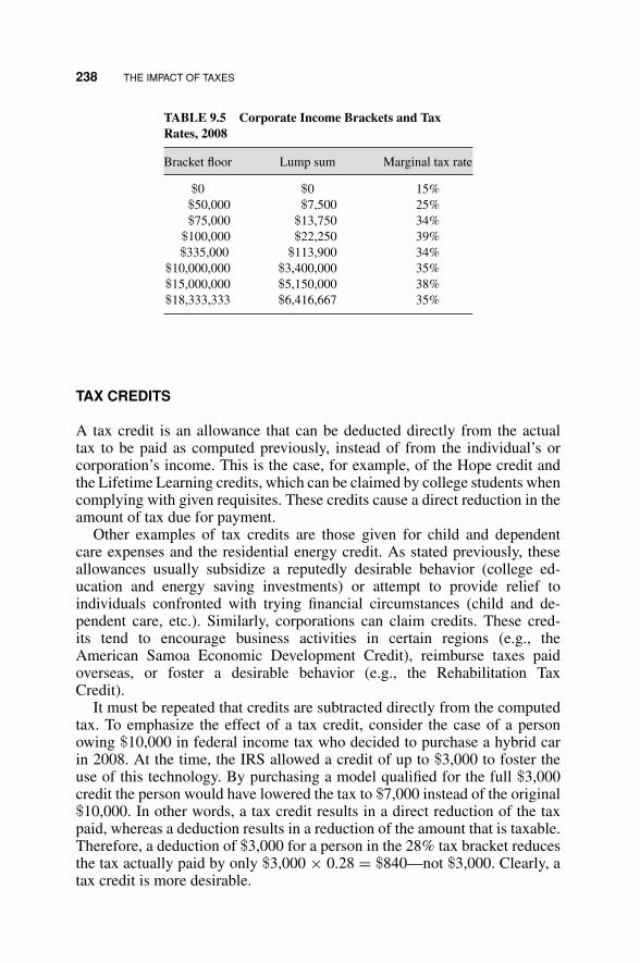
P1: OTA/XYZ P2: ABC



TABLE 9.5 Corporate Income Brackets and TaxRates, 2008

Bracket floor Lump sum Marginal tax rate

$0 $0 15%$50,000 $7,500 25%$75,000 $13,750 34%

$100,000 $22,250 39%$335,000 $113,900 34%

$10,000,000 $3,400,000 35%$15,000,000 $5,150,000 38%$18,333,333 $6,416,667 35%

TAX CREDITS

A tax credit is an allowance that can be deducted directly from the actualtax to be paid as computed previously, instead of from the individual’s orcorporation’s income. This is the case, for example, of the Hope credit andthe Lifetime Learning credits, which can be claimed by college students whencomplying with given requisites. These credits cause a direct reduction in theamount of tax due for payment.

Other examples of tax credits are those given for child and dependentcare expenses and the residential energy credit. As stated previously, theseallowances usually subsidize a reputedly desirable behavior (college ed-ucation and energy saving investments) or attempt to provide relief toindividuals confronted with trying financial circumstances (child and de-pendent care, etc.). Similarly, corporations can claim credits. These cred-its tend to encourage business activities in certain regions (e.g., theAmerican Samoa Economic Development Credit), reimburse taxes paidoverseas, or foster a desirable behavior (e.g., the Rehabilitation TaxCredit).

It must be repeated that credits are subtracted directly from the computedtax. To emphasize the effect of a tax credit, consider the case of a personowing $10,000 in federal income tax who decided to purchase a hybrid carin 2008. At the time, the IRS allowed a credit of up to $3,000 to foster theuse of this technology. By purchasing a model qualified for the full $3,000credit the person would have lowered the tax to $7,000 instead of the original$10,000. In other words, a tax credit results in a direct reduction of the taxpaid, whereas a deduction results in a reduction of the amount that is taxable.Therefore, a deduction of $3,000 for a person in the 28% tax bracket reducesthe tax actually paid by only $3,000 × 0.28 = $840—not $3,000. Clearly, atax credit is more desirable.

P1: OTA/XYZ P2: ABC


MARGINAL, AVERAGE, AND EFFECTIVE TAX RATES 239

TAX PAYROLL WITHHOLDING

Employers are required to retain an amount from each paycheck that is roughlyenough to cover the employee’s tax liability at the end of the year. Thiswithholding tax reduces the impact of the thousands of dollars levied in taxesto any average employee. The amount held back is essentially an escrowaccount held for the employee by the employer. At the time of payment, thisescrow, or withheld, amount provides the employee with a basis for payingtax. As many taxpayers know, it often occurs that the total retention exceedsthe total tax owed, in which case the IRS refunds the amount of over paymentto the individual taxpayer.

TAX PAYMENT SCHEDULES

Corporations and some individuals must pay their taxes in quarterly install-ments, although their deadlines are slightly different. The requirement to makequarterly payments is similar, in concept, to withholding taxes for the indi-vidual employee discussed in the previous section. Installments are intendedto avoid the situation of a company being confronted with a large payment atthe end of the tax period. It ensures that companies and individuals “pay asthey go” and spread tax payments over the tax period. This avoids the shockof paying a single large “balloon” payment at the end of the tax period.

Corporations can select a fiscal year, which does not need to coincide withthe calendar year. While a calendar year ends on December 31st, a corporatefiscal year can end on any arbitrary date, usually at the end or the middleof a month. Many retailers, for example, do not like a December 31st fiscalyear end because they are still occupied with the busy Christmas season.Nevertheless, about two thirds of American corporations choose to havetheir fiscal year end with the calendar year. A corporation with this calendarmust estimate its profit and submit installments on the 15th of April, June,September, and December. Proprietorships and other organizational formswithout an independent tax standing, as well as individuals with substantialincome that is not subject to withholding, use the same calendar for thefirst three installments (15th of April, June, and September) but pay the lastinstallment on January 15th of the following year. Oddly enough, this meansthat there are 2 months between the 1st and 2nd payments, 3 months betweenthe 2nd and 3rd payment, and 4 months between the 3rd and last payment.

MARGINAL, AVERAGE, AND EFFECTIVE TAX RATES

The previous discussions of taxable income and tax computations yield insightabout the tax paid by an individual or corporation compared to its income. Asmentioned before, a progressive system imposes more taxes as a percentage

P1: OTA/XYZ P2: ABC



of income on higher income. But, it is also important to view taxes as apercentage of the money earned by the taxpayer.

� The marginal tax rate is the percentage that an additional dollar earnedby a taxpayer would have to pay. The marginal tax rate is relevant tocorrectly analyze the money saved or paid by relatively small changes inincome. In the discussion of organizational forms, it was mentioned inthe partnership form that Elmer Fudd (married filing jointly) would earn$102,000 and pay taxes for around $13,713 as a partner in a partnership.Table 9.3 shows that for a couple filing jointly, this income belongs tothe bracket taxed at 25%, that is, its marginal tax rate would be 25%.This means that if he decides to give $1,000 to charity, he will be able toreduce his taxes by 25% × $1,000 = $250.

� The average tax rate is the ratio of total taxes paid to taxable income.The average tax rate paid by any individual with income over the min-imum bracket will always be lower than the marginal rate, since theaverage includes the fraction of the income taxed at the lower tax rateof the low-income brackets. This is not true for corporations, as canbe observed in its convoluted table. Returning to Mr. Fudd, his taxableincome would be $102,000 (gross adjusted income) − $10,900 (std. de-duction) – 2 × $3,500 = $84,100. Therefore, his average tax rate wouldbe $13,713/$84,100 = 16.3%.

� The effective tax rate results from dividing the amount of paid taxes bythe income without considering deductions or exemptions. Elmer Fuddhad an effective rate of $13,713/$102,000 = 13.4%. The spread betweenaverage and effective income taxes is low in this case, compared to manylarge corporations with large tax breaks. The IRS reported that in 1999the effective rate paid (in average) by the top 10,000 largest corporationswas 20%, considerably less than their average tax rate of near 34%.

NET OPERATING LOSSES

A company has a net operating loss (NOL) when it reports a higher amount ofallowable deductions than revenue. NOL is generally close, but not equal, tothe loss (if any) reported in the company’s Income Statement. As previouslydiscussed, there are deductions for tax purposes that may be computed dif-ferently in the company’s accounting system (e.g., depreciation) and may notappear in the Income Statement (e.g., incentives to locate in certain areas), orvice versa, may not be acceptable for tax purposes (e.g., some public relationsand travel expenses). Individuals and all forms of business organizations canreport a NOL.

No income taxes are levied in the year that an individual or company hasan NOL. Furthermore, the loss can be used to revise the taxable income of

P1: OTA/XYZ P2: ABC


NET OPERATING LOSSES 241

previous years and to lower the taxable income of future years. The NOLapplied to past years is called a carryback, and the amount applied to futureyears is a carryforward.

The rules applied to carryback and carryforward have changed with everymajor revision of the tax code, and depend on the type of loss, income, andeven the institution (banks, for example, have their set of rules in this area).Being aware of the concepts of carryback and carryover should be enough forthe intended level of this book. Carryback has been limited to the previous3 years and carry forward to the next 15 years for most situations applicableto construction companies. The following example helps in the understandingof the process.

Suppose that a company reports a NOL of $1,000,000 for 2009. It had ataxable income of $200,000 in each of the previous four years. How wouldthis company apply this NOL to revise previous tax computations and as adeduction for coming years?

The carryback process is usually performed before the carryforward, be-cause it results in immediate tax relief (a refund) from the IRS. An excep-tion happens when a company finds that the marginal tax rate of previousyears is lower than the expected marginal rate for coming years. In such a(uncommon) case, the difference in rates may justify the wait. In this example,the company chooses to apply the carryback first. The taxable income of eachof the three previous years is revised to zero:

� In 2008, the amount available to carry back is $1,000,000. After sub-tracting the $200,000 originally reported as taxable income, the revisedtaxable income is zero, and the amount available to further carryback is$800,000.

� In 2007, the revised taxable income is also zero, and the remainingcarryback is $600,000.

� In 2006, the same process is applied. The revised taxable income is zero,and the remaining carryback is $400,000

� The taxable income for 2005 cannot be revised, despite the $400,000 ofNOL still available, since this year is more than 3 years before the NOL.

The company will send the IRS revised tax returns showing zero taxableincome for 2008, 2007, and 2006. It will get a refund for all taxes paid inthose years (not $200,000 for each year but the tax amount paid in each year).

The unapplied portion of the NOL is saved as carryforward for the comingyears. If the company has a taxable income before applying the NOL of$100,000 in 2010, it can set to zero the taxable income and still have $300,000available. If it has a taxable income of $450,000 in 2011, it would apply all theremaining funds from the NOL to pay taxes on a taxable income of $150,000.

P1: OTA/XYZ P2: ABC



TAXES ON DIVIDENDS AND LONG-TERM CAPITAL GAINS

Dividends, as discussed in the accounting section of this book, are the pay-ments made by a corporation to its shareholders. They are the portion of thecorporation’s profit not reinvested as retained earnings.

As noted in the section entitled “Straight Line Method,” when a capitalasset is held for more than a year and then sold at a higher price than itsdepreciated or base value, the resulting profit is called a long-term capitalgain. An asset such as a piece of equipment or a building, typically appear inthe Non-Current Assets section of a company’s balance sheet. To qualify as along-term capital gain, the capital asset cannot be purchased for the purposeof being resold.

Dividends and long-term capital gains are taxed under different rules.Currently, a flat tax of 15% is levied for dividends, as well as for long-termcapital gains with the exception of real estate.5 Since this part of a company’sor individual’s income is treated differently, dividends and long-term capitalgains are not counted in the regular income tax computations discussed so far.

There are several types of capital gains that result in different rates. Long-term gains involving real estate are taxed at up to 25%, and collectibles atup to 28%. Short-term capital gains (those from capital assets held for lessthan a year) and stock in many small businesses are taxed at the marginalrate of regular income. Complicating this topic, current rates are scheduledto expire in 2010, making these specifics moot unless new legislation extendstheir term.

ALTERNATIVE MINIMUM TAX

The tax rules discussed so far can result in some wealthier individuals and cor-porations paying proportionally less taxes than lower-income taxpayers. TheAlternative Minimum Tax (AMT) amounts to a parallel set of rules designedto avoid any tax loopholes in the federal tax system. This is accomplishedby a simpler, flatter system, which sets the individual or corporation taxableincome at a level much closer to their income as computed by accountingstandards. In other words, it allows fewer exemptions to individuals and cor-porations falling under its scope. Its tax rates are nearly flat: 26–28% forindividuals, 20% for corporations. If an individual or corporation has a highlevel of income, it must perform the AMT calculations. The amount owedwill be the higher of the tax owed using the regular approach or the AMT.

The AMT was first applied in 1970 and revised in 1986. Its original scopemade it applicable to literarily a few dozen very wealthy families and a fewhundred large corporations. Unfortunately, its underlying legislation does notinclude a provision to adjust for inflation, and its thresholds have become

5 Individuals with taxable income falling in the 10% or 15% brackets of their applicable tax table aresubject to a long-term capital gain/dividend rate of 5% instead of 15%.

P1: OTA/XYZ P2: ABC



so low that an upper-middle income family may find itself dealing with thisparallel system. A Faustian dilemma has developed. Although it is clear thatthe AMT is changing its fundamental purpose by including upper-middle-class families, cutting off the tax revenue generated from the AMT paid bythese families would lead to a reduction of billions of dollars now paid intothe coffers of the government.

The corporate AMT is more complex than the individual version. It is notapplicable to small corporations and has its own set of deductions (prefer-ences) and allows the equivalent of a “personal exemption” that is tapered offfor higher alternative minimum taxable incomes (AMTI)

In order to deal with this and a host of other tax-related issues, evenrelatively small construction firms organized in the corporate form, requirethe service of experienced tax professionals.

SUMMARY

This chapter has discussed issues related to taxation that influence the bot-tom line of a construction company and impact financial decisions. Clearly,minimizing the amount of taxes paid increases the profit and retained earn-ings controlled by the company and ultimately distributed to the owners andstockholders. One area, which is often discussed in conjunction with taxa-tion, is contributions made by companies to ensure the welfare of employees.Companies are involved in paying Social Security contributions required byfederal law, Unemployment and Workers’ Compensation insurance requiredby state governments, and so-called “fringe” benefits required of union con-tractors by union contracts. Although these are not strictly taxes, they do havea similar impact on the profitability of the company and must be carefullyanalyzed. A cursory introduction to these charges and how they impact laborcosts is presented in Construction Management by Halpin published by JohnWiley and Sons, Inc. (Halpin, 2006). The company’s top management, andparticularly the chief financial officer (CFO), must continuously study andanalyze the impact of taxation on all financial and organizational decisions.Taxes are business costs which lead to a 34% reduction in before tax incomeand must be considered very seriously. These costs require at least the samelevel of professional and financial expertise that is required from a technicalperspective to build innovative and successful construction projects.


1. Explain in your own words the concept of marginal tax rate.2. Does a single individual making $500,000 pay the same marginal tax

rate as another making $1,000,000? Explain.3. You decide to sell a house that you bought five years ago with the purpose

of renting it. Its purchase price was $300,000, and now its market value

P1: OTA/XYZ P2: ABC



is about $500,000. How much should you expect to pay in taxes for thesale of this house?

4. What is the average tax rate paid by a single person with a $60,000 AGIfor 2008?

5. What is the name of the amount of money that can be deducteddirectly from the computed tax, instead of from the gross adjustedincome?

6. Which business enterprises pay untaxed profits to owners/partners whothen pay the taxes on their individual returns?

7. Peachtree Construction Inc., which is incorporated as a corporation, re-ported a net operating loss (NOL) of $500,000 in 2008. Given the follow-ing data, how much of this NOL is likely to be available as a deductionfrom its profit in 2009?� The company was created in 2006.� It had a NOL of $100,000 in 2006.� It reported a profit before taxes of $400,000 in 2007.

8. A corporation had a net income before taxes of $1,200,000 for 2008.Find the tax liability for this company.

9. Pegg Construction, a partnership of three brothers, had a net incomebefore taxes of $300,000. The brothers have agreed that all profit willbe shared in equal parts. John Pegg is single, and has an income of$500,000 from other sources. How much will Mr. Pegg pay in taxes forthe $100,000 from the partnership with his siblings?

10. Let us assume that we own our personal residences. One question ofinterest is, “If we depreciate real property (e.g. land, buildings, etc.),can we depreciate the house in which we live?” Depreciation allows forthe recovery of the cost of doing business. Since, in most cases, we donot “do business” in our home, our residence is not a depreciable asset.You can, however, think of some instances in which a person conductsbusiness at home. Can such a person working at home, depreciate thecost of his/her house?

11. Why are governments willing to agree to accept the concept of deprecia-tion, which leads in many cases to a considerably lower level of taxationfor business entities? The answer to this question provides an insightinto how modern economies operate. How are economies impacted bydepreciation?

12. Verify the 5- and 7-year property class percentages given in Table 9.2 byapplying the 200% DB approach to a piece of equipment with a nominalvalue of $1,000. For the 7-year property class, in what year is the switchfrom 200% DB to Straight Line made based on the percentages in theTable 9.2. Only half of the first and last years are considered in thecomputations. This means that for a five-year class property, only halfthe 200% DB amount (40%/2 = 20%) is deducted.

P1: OTA/XYZ P2: ABC



13. Why do you think the 150% DB method is used as the basis fordepreciation for 15- and 20-year classes of equipment, as given inTable 9.2?

14. Find the yearly depreciation of a $100,000 five-year class concrete mixer,first assuming that it is new when purchased, and then that it is purchasedas used equipment.

P1: OTA/XYZ P2: ABC

JWBT106-APP-A JWBT106-Halpin June 26, 2009 9:45 Printer: Sheridan Books

APPENDIX A

TYPICAL CHART OF ACCOUNTS

TABLE A.1 General Ledger Accounts

Assets

10. Petty cash11. Bank deposits

.1 General bank account

.2 Payroll bank account

.3 Project bank accounts

.412. Accounts receivable

.1

.2 Parent, associated, or affiliated companies

.3 Notes receivable

.4 Employees’ accounts

.5 Sundry debtors

.613. Deferred receivables

All construction contracts are charged to this account, being diminished byprogress payments as received. This account is offset by Account 48.0,Deferred Income.

14. Property, plant, and equipment

Property and General Plant

.100 Real estate and improvements

.200 Leasehold improvements

.300 Shops and yards

(continued )

247



P1: OTA/XYZ P2: ABC


248 TYPICAL CHART OF ACCOUNTS

TABLE A.1 (Continued )

Mobile Equipment

.400 Motor vehicles

.500 Tractors.01 Repairs, parts, and labor.05 Outside service.12 Tire replacement.15 Tire repair.20 Fuel.25 Oil, lubricants, filters.30 Licenses, permits.35 Depreciation.40 Insurance.45 Taxes

.510 Power shovels

.520 Bottom dumps

Stationary Equipment

.530 Concrete mixing plant

.540 Concrete pavers

.550 Air compressors .560

Small Power Tools and Portable Equipment

.600 Welders

.610 Concrete power buggies

.620 Electric drills .630

Marine Equipment

.700

Miscellaneous Construction Equipment

.800 Scaffolding

.810 Concrete forms

.820 Wheelbarrows

.830

Office and Engineering Equipment

.900 Office equipment

.910 Office furniture

.920 Engineering instruments15. Reserve for depreciation16. Amortization for leasehold17. Inventory of materials and supplies

.1 Lumber

.2 Hand shovels

P1: OTA/XYZ P2: ABC


TYPICAL CHART OF ACCOUNTS 249

TABLE A.1

.3 Spare parts

.4These accounts show the values of all expendable materials and supplies.Charges against these accounts are made by authenticated requisitionsshowing project where used.

18. Returnable deposits.1 Plan deposits.2 Utilities.3

Liabilities

40. Accounts payable41. Subcontracts payable42. Notes payable43. Interest payable44. Contracts payable45. Taxes payable

.1 Old-age, survivors, and disability insurance (withheld from employees’ pay)

.2 Federal income taxes (withheld from employees’ pay)

.3 State income taxes (withheld from employees’ pay)

.446. Accrued expenses

.1 Wages and salaries

.2 Old-age, survivors, and disability insurance (employer’s portion)

.3 Federal unemployment tax

.4 State unemployment tax

.51 Payroll insurance (public liability and property damage)

.52 Payroll insurance (workmen’s compensation)

.6 Interest

.747. Payrolls payable48. Deferred income49. Advances by clients

Net Worth

50. Capital stock51. Earned surplus52. Paid-in-surplus53.

Income

70. Income accounts.101 Project income.102.2 Cash discount earned

(continued )

P1: OTA/XYZ P2: ABC


250 TYPICAL CHART OF ACCOUNTS

TABLE A.1 (Continued )

.3 Profit or loss from sale of capital assets

.4 Equipment rental income

.5 Interest income

.6 Other income

Expense

80. Project expense.100 Project work accounts.700 Project overhead accounts

These are control accounts for the detail project cost accounts that aremaintained in the detail cost ledgers.

81. Office expense.10 Officer salaries.11 Insurance on property and equipment.20 Donations.21 Utilities.22 Telephone and telegraph.23 Postage.30 Repairs and maintenance

82. Yard and warehouse expense (not assignable to a particular project).10 Yard salaries.11 Yard supplies

83. Estimating department expense accounts.10 Estimating salaries.11 Estimating supplies.12 Estimating travel

84. Engineering department expense accounts .1085. Cost of equipment ownership

.1 Depreciation

.2 Interest

.3 Taxes and licenses

.4 Insurance

.5 Storage86. Loss on bad debts87. Interest90. Expense on office employees

.1 Workmen’s compensation insurance

.2 Old-age, survivors, and disability insurance

.3 Employees’ insurance

.4 Other insurance

.5 Federal and state unemployment taxes

.691. Taxes and licenses

.1 Sales taxes

.2 Compensating taxes

.3 State income taxes

.4 Federal income taxes

P1: OTA/XYZ P2: ABC

JWBT106-APP-B JWBT106-Halpin June 26, 2009 17:2 Printer: Sheridan Books

APPENDIX B

FURTHER ILLUSTRATIONSOF TRANSACTIONS

TABLE B.1 Composite of Ledger Entries 1–20

Cash Accounts Receivable

DR + CR − DR + CR −$ 50,000(1) $330,000(5)

50,000(1) 5,000(5) $414,000(2)360,000(4) 85,000(5) 112,500(2)20,000(4) 2,000(5) $360,000(4)90,000(4) 11,000(9) 27,000(6) 90,000(4)6,000(4) 2,250(10) 20,000(7)5,000(7) 33,500(11)

20,000(7) 3,160(13)4,000(20)

Retainage Receivable Accrued Interest Receivable

DR + CR − DR + CR −$46,000(2) $4,000(19)

12,500(2) $4,000(20)$20,000(4)

6,000(4)3,000(6) 5,000(7)

(continued )

251



P1: OTA/XYZ P2: ABC


252 FURTHER ILLUSTRATIONS OF TRANSACTIONS

TABLE B.1 (Continued )

Work-in-Progress Expense (Asset)* Prepaid Insurance

DR + CR − DR + CR −$370,000(3) $7,200(14)

100,000(3)11,000(8)2,250(10)

Fixed Assets Accumulated Depreciation

DR + CR − DR + CR −$90,000(16) $7,500(18)

Accounts Payable Accrued Liability

DR − CR + DR − CR +$340,000(3) $3000(15)

92,000(3) 4800(17)$330,000(5)

85,000(5)10,000(8)

10,000(9) 3,160(12)3,160(13) 7,200(14)

Retainage Payable Billings in Excess of Revenues

DR − CR + DR − CR +$30,000(3)

8,000(3)$5,000(5)

2,000(5)1,000(9) 1,000(8)

Notes Payable—Short-term Notes Payable-Long-Term

DR − CR + DR + CR −$30,000(16) $60,000(16)

*This expense account is a nominal account used to capture expenses on jobs in progress pendingreconciliation at closing of accounts. These expenses are viewed as assets until closed to the real account,“contract expense.” This occurs at the end of the accounting period.

P1: OTA/XYZ P2: ABC


FURTHER ILLUSTRATIONS OF TRANSACTIONS 253

TABLE B.1

Advanced Billings Retained Earnings

DR − CR + DR + CR −$460,000(2)

125,000(2)30,000(6)

Capital-Common Stock

DR − CR +$50,000(1)

50,000(1)

Project Revenue (Sales) Project Expense

DR − CR + DR − CR +

General Overhead

DR − CR +$33,500(11)

3,160(12)3,000(15)

Interest Income Interest Expense

DR − CR + DR + CR −$4000(19) $4800(17)

Depreciation Expense

DR + CR −$7500(18)

P1: OTA/XYZ P2: ABC



Liabilities Revenue

Revenue

Revenue

Revenue

Revenue

Revenue

Revenue

Project

B

Project

A

Home

office

Expense

Expense

Expense

Expense Expense

Expense

Expense

Retained earnings

(end of period)

Balance sheet

(31 Dec 20x1)

Transaction 1

Income statement(4th qtr 20x1)

Revenue

Expense

R.E.

Asset (ledger)

accounts

D+

Equipment

Cash

50,000

50,000

50,000

50,000

50,000

50,000

50,000

50,000

Liability (ledger)

accountsNet worth

accounts

Capital stock

Initial

capitalR. Jones

Description of transaction: Initial capital to form Apex Construction Company is contributed

by R. Jones and M. Jackson. Each contributes $50,000. Stock in the amount of 10,000 sharesis issued to each.

DescriptionJournal entry:

Cash

Capital stock–R. Jones Cash

Capital stock–M. Jackson

DR CR

Initialcapital

M. Jackson

Accounts payable

D+

C–

D+ C–

D+ C–

C–

D+ C–

D+

D–

C–

C+

D– C+

D– C+

D– C+

D– C+

Real property

Assets Net worth

Retained

earnings

Figure B.1

P1: OTA/XYZ P2: ABC



Liabilities Revenue

Revenue

Revenue

Revenue–project B

Revenue–project A

Revenue

Project

B

ProjectA

Home

office

Expense

Expense

Expense

Expense

Expense–project B

Expense–project A

125,000

429,677

Retained earnings

(end of period)

Balance sheet

(31 Dec 20x1)

Transaction 2


Revenue

Expense

R.E.

Asset (ledger)

accounts

D+

Equipment

Accounts receivable

Retainage receivable

Liability (ledger)

accounts

Accounts payable Capital stock

Billings–B

Billings–A

Billings in excess of

costs and estimatedearnings

Net worthaccounts

414,000112,500

12,50046,000

D+

C–

D+ C–

D+ C–

C–

D+ C–

D+ C–

D+ C–

D– C+

D– C+

D– C+

D– C+ D– C+

D– C+

D– C+

D– C+

30,323

125,000

460,000

Description

Accounts receivable

Retainage receivableBillings–project A

Accounts receivableRetainage receivable

Billings–project B

Billings–project A

Revenue–project ABillings in excess of costs

and estimated earningsBillings–project B

Revenue–project B

CRDR

414,000

46,000

112,500

12,500

429,677

30,323

125,000

460,000

125,000

460,000

125,000

Accumulation of

entries to billings

through period

Closing entries

Description of transaction: The billings on projects A and B for the year 20x1 are shown posted based on

the percentage-of-completion method. The actual billed amounts on A and B are $460,000 and $125,000,respectively. A retainage of 10 percent is held on each contract. Although many individual billings would bemade over the year, they have been consolidated into single entries for the purpose of this illustration. Thecalculated revenues on A and B (with POC) are $429,677 and $125,000, respectively. The overbilling onA is accounted for in the liability account Billings in excess of costs and estimated earnings.

429,677

30,323

125,000

Real property

Assets Net worth

Retained

earnings

Invoices–

billingsproject A$460,000

Invoices–

billingsproject B$125,000

Figure B.2

P1: OTA/XYZ P2: ABC



Liabilities Revenue

Revenue

Revenue 100,000

Revenue

Project

B

ProjectA

Home

office

Expense

Expense

Expense

Expense

Expense–project B

Expense–project A

370,000

Retained earnings

(end of period)

Balance sheet

(31 Dec 20x1)

Transaction 3


Revenue

Expense

R.E.

Asset (ledger)

accounts

D+

Equipment

WIP–project B

WIP–project A

100,000

100,000

Liability (ledger)

accounts


Expense

voucher,project B

$100,000

Net worth

accounts

370,000 370,000

D+

C–

D+ C–

D+ C–C–

D+ C–

D+ C–

D+ C–

D– C+

D– C+

D– C+

D– C+

D– C+

92,000

340,000

8,00030,000

D– C+


WIP– expenses–project A Accounts payable Retainage payable

WIP– expenses–project B Accounts payable

Retainage payable

Project expenses–project A

Project expenses–project BWIP–expense–project A

WIP–expense–project B

CRDR

340,00030,000

92,0008,00

370,000

100,000

370,000100,000

370,000100,000

Accumulation of

expense duringthe period

Closing actions

Description of transaction: The cost of projects A and B for the year 20x1 are $370,000 and $100,000, respectively.

Retainage amounts of $30,000 and $8,000 respectively, on A and B are held by Apex from subcontract billings. Thesecosts are carried as expenses under the appropriate project expense accounts. Although the costs would accumulatefor many individual transactions through the year, they are shown as single lump sum entries in this example.

Real property

Assets Net worth

Retained

earnings

Retainage payable

Expense

voucher,project A

$370,000

Figure B.3

P1: OTA/XYZ P2: ABC



Liabilities

Balance sheet

(31 Dec 20x1)

Assets Net worth

Retainedearnings

Revenue

Project

B

Project

A

Expense

Retained earnings

(end of period)

Transaction 4


Revenue

Expense

R.E.

Revenue

Revenue

Home

office

Expense

Revenue

Expense

Expense

D+ C–

D+ C–

D+ C–

D– C+

D– C+

D– C+

Liability (ledger)

accounts


Net worthaccounts

D– C+ D– C+

Asset (ledger)accounts

Equipment

D+ C–

Cash

D+

90,000360,000

20,0006,000

C–

D+ C–

Real property

D+ C–

20,000

6,000


Collectables

D+ C–

360,00080,000

Journal entry: Description DR CR

360,000

20,000

90,000

6,000

Cash

Cash

Cash

Cash

360,000

20,000

90,000

6,000

Accounts receivable


Accounts receivable


Accounts receivable

Description of transaction: Payments received on project A from client amount to $360,000 in billings

and $20,000 in retainage. Payments received on project B amount to $90,000 in billings and $6,000 in retainage. These are accumulations of individual collections during the year.

Figure B.4

P1: OTA/XYZ P2: ABC



Description of transaction: Payments to vendors and subcontractors on project A amount to $330,000 inregular payments and $5,000 in retainage during period. Payments to vendors and subcontractors on

Project B amount to $85,000 in regular payments and $2,000 in retainage during the period.

Liabilities

Balance sheet

(31 Dec 20x1)

Assets Net worth

Retained

earnings

Revenue

Project

B

Project

A

Expense

Retained earnings

(end of period)

Transaction 5


Revenue

Expense

R.E.

Revenue

Revenue

Home

office

Expense

Revenue

Expense

Expense

D+ C–

D+ C–

D+ C–

D– C+

D– C+

D– C+


Equipment

D+ C–

Cash

D+

330,00085,0005,0002,000

330,00085,000

C–

D+ C–

Real property

Liability (ledger)

accounts

Accounts payable

Payments

on projects

Capital stock

Net worthaccounts

D– C+

5,0002,000

Retainage payable

D– C+

D– C+


330,000

5,000

85,000

2,000

Cash

Cash

Cash

Cash

330,000

5,000

85,000

2,000

Accounts payable–A

Retainage payable–A

Accounts payable–B

Retainage payable–B

$

Figure B.5

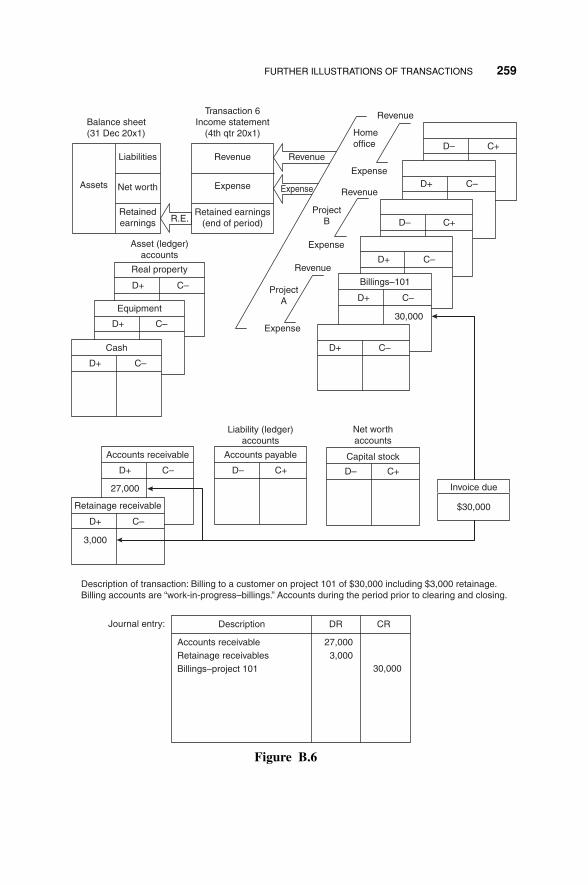
P1: OTA/XYZ P2: ABC



Liabilities

Balance sheet

(31 Dec 20x1)

Assets Net worth

Retained

earnings

Revenue

Project

B

Project

A

Expense

Retained earnings

(end of period)

Transaction 6


Revenue

Expense

R.E.

Revenue

Revenue

Home

office

Expense

Revenue

Billings–101

Expense

Expense

D+ C–

D+ C–

D+ C–

D– C+

D– C+

D+ C–

30,000


Equipment

D+ C–

Cash

D+ C–

D+ C–

Real property

Liability (ledger)

accounts


Net worthaccounts

D– C+

Accounts receivable

D+

27,000

C–


D+

3,000

C–

D– C+


27,000

3,000

30,000

Accounts receivable

Retainage receivables

Billings–project 101

Description of transaction: Billing to a customer on project 101 of $30,000 including $3,000 retainage.Billing accounts are “work-in-progress–billings.” Accounts during the period prior to clearing and closing.

Invoice due

$30,000

Figure B.6

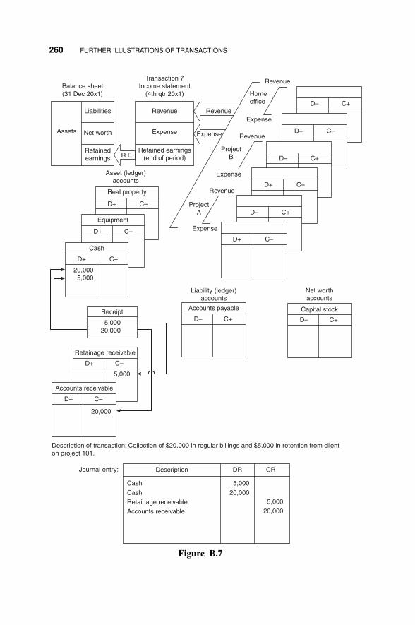
P1: OTA/XYZ P2: ABC



5,000


D+ C–

20,000

Accounts receivable

D+ C–

Liabilities

Balance sheet

(31 Dec 20x1)

Assets Net worth

Retained

earnings

Revenue

Project

B

Project

A

Expense

Retained earnings

(end of period)

Transaction 7

Income statement

(4th qtr 20x1)

Revenue

Expense

R.E.

Revenue

Revenue

Home

office

Expense

Revenue

Expense

Expense

D+ C–

D+ C–

D+ C–

D– C+

D– C+

D– C+

Asset (ledger)

accounts

Equipment

D+ C–

Cash

D+

20,000

5,000

C–

D+ C–

Real property

Liability (ledger)

accounts

Accounts payableReceipt

5,000

20,000

Capital stock

Net worth

accounts

D– C+ D– C+

Description of transaction: Collection of $20,000 in regular billings and $5,000 in retention from client

on project 101.


5,000

20,000

5,000

20,000

Cash

Cash


Accounts receivable

Figure B.7

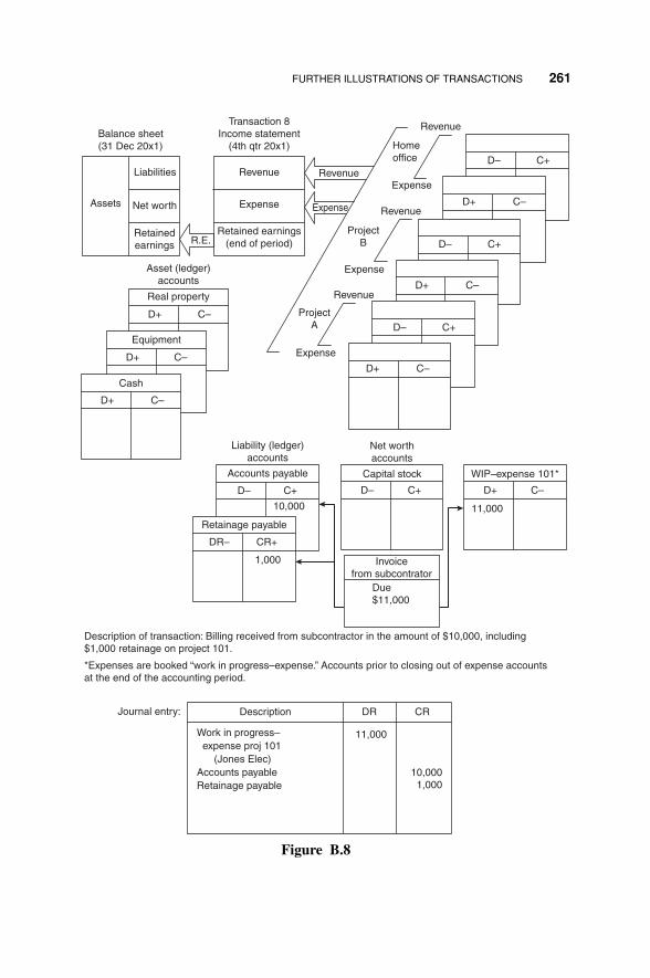
P1: OTA/XYZ P2: ABC



Liabilities

Balance sheet

(31 Dec 20x1)

Assets Net worth

Retained

earnings

Revenue

Project

B

ProjectA

Expense

Retained earnings

(end of period)

Transaction 8


Revenue

Expense

R.E.

Revenue

Revenue

Home

office

Expense

Revenue

Expense

Expense

D+ C–

D+ C–

D+ C–

D– C+

D– C+

D– C+


Equipment

D+ C–

Cash

D+ C–

D+ C–

Real property

10,000 11,000

Liability (ledger)accounts


Net worthaccounts

D– C+

1,000

Retainage payable

DR– CR+

D– C+

WIP–expense 101*

D+ C–


Work in progress–

expense proj 101

(Jones Elec)

Accounts payable

Retainage payable

11,000

10,000

1,000

Description of transaction: Billing received from subcontractor in the amount of $10,000, including$1,000 retainage on project 101.

*Expenses are booked “work in progress–expense.” Accounts prior to closing out of expense accountsat the end of the accounting period.

Invoicefrom subcontrator

Due$11,000

Figure B.8

P1: OTA/XYZ P2: ABC



Liabilities Revenue

Revenue

Revenue

Revenue

Project

B

ProjectA

Home

office

Expense

Expense

Expense

Expense

Retained earnings

(end of period)

Balance sheet

(31 Dec 20x1)

Transaction 9

Income statement

(4th qtr 20x1)

Revenue

Expense

R.E.


D+

Equipment

Cash

To

subcontractors

Liability (ledger)

accounts


Net worth

accounts

11,000

D+

C–

D+ C–

D+ C–

C–

D+ C–

D+ C–

D– C+

D– C+

D– C+

D– C+

D– C+

10,000

1,000

D– C+


Accounts payable

Retainage payable

Cash

CRDR

10,000

1,000

11,000

Description of transaction: Payment of $10,000 in regular billings and $1,000 in retainage on project 101.

Subcontractor billings received previously.

Real property

Assets Net worth

Retained

earnings

Retainage payable$

Figure B.9

P1: OTA/XYZ P2: ABC



Liabilities Revenue

Revenue

Revenue

Revenue

ProjectB

ProjectA

Homeoffice

Expense

Expense

Expense

Expense

Retained earnings(end of period)

Balance sheet(31 Dec 20x1)

Transaction 10


Revenue

Expense

R.E.


D+

Equipment

Cash

To workers



Net worthaccounts

2,250

D+

C–

D+ C–

D+ C–

C–

D+ C–

D+ C–

D– C+

D– C+

D– C+

D– C+ D– C+

WIP–expense 101

D+ C–


WIP–expense

Job 101

(payroll)

Cash

CRDR

2,250

2,250

Description of transaction: Payment of weekly salary for craft workers on project 101 in the amount of$2,250.

Real property

Assets Net worth

Retainedearnings

$

2,250

Figure B.10

P1: OTA/XYZ P2: ABC



Liabilities Revenue

Revenue 33,500

Revenue

Revenue

ProjectB

ProjectA

Homeoffice

Expense

Expense

Expense

Expense General overhead



Transaction 11


Revenue

Expense

R.E.


D+

Equipment

Cash

To home officestaff



Net worthaccounts

33,500

D+

C–

D+ C–

D+ C–

C–

D+ C–

D+ C–

D– C+

D– C+

D– C+

D– C+ D– C+


General overhead

(monthly home office salary)

Cash

CRDR

33,500

33,500

Description of transaction: Payment of home staff for month of June in the amount of $33,500.

Real property

Assets Net worth

Retainedearnings

$

Figure B.11

P1: OTA/XYZ P2: ABC



Liabilities Revenue

Revenue 3,160

Revenue

Revenue

ProjectA

ProjectB

Homeoffice

Expense

Expense

Expense




Transaction 12


Revenue

Expense

R.E.


D+

Equipment

Cash



Net worthaccounts

D+

C–

D+ C–

D+ C–

C–

D+ C–

D+ C–

D– C+

D– C+

D– C+

D– C+

$3,160

D– C+


General overhead

(heating)

Accounts payable

CRDR

$3,160

$3,160

Description of transaction: Invoice for home office costs for heating headquarters building in the amountof $3,160.

Real property

Assets Net worth

Retainedearnings

Invoice

gas company

$3,160

Figure B.12

P1: OTA/XYZ P2: ABC



Liabilities Revenue

Revenue

Revenue

Revenue

ProjectB

ProjectA

Homeoffice

Expense

Expense

Expense

Expense



Transaction 13


Revenue

Expense

R.E.


D+

Equipment

Cash

To gascompany



Net worthaccounts

3,160

D+

C–

D+ C–

D+ C–

C–

D+ C–

D+ C–

D– C+

D– C+

D– C+

D+ C– D+ C–

3,160


Accounts payable

(city gas company)

Cash

CRDR

3,160

3,160

Description of transaction: Payment of invoice in Transaction 12.

Real property

Assets Net worth

Retainedearnings

$

Figure B.13

P1: OTA/XYZ P2: ABC



Liabilities Revenue

Revenue

Revenue

Revenue

ProjectB

ProjectA

Homeoffice

Expense

Expense

Expense

Expense



Transaction 14


Revenue

Expense

R.E.


D+

Equipment

Cash



Net worthaccounts

Invoice

$7,200

Ajax insurance

D–

C–

D+ C–

D+ C–

C+

D+ C–

D+ C–

D– C+

D– C+

D– C+

D– C+

7,200

D– C+

Prepaid insurance

D+ C–


Prepaid insurance

Accounts payable

CRDR

Decsription of transaction: An invoice for insurance for the coming year is received in the amountof $7,200. The payment represents a prepayment of insurance.

Real property

Assets Net worth

Retainedearnings

7,200

7,200

7,200

Figure B.14

P1: OTA/XYZ P2: ABC



Liabilities Revenue

Revenue

Revenue

Revenue

ProjectA

ProjectB

Homeoffice

Expense

Expense

Expense




Transaction 15


Revenue

Expense

R.E.


D+

3,000

Equipment

Cash



Net worthaccounts

D+

C–

D+ C–

D+ C–C–

D+ C–

D+ C–

D– C+

D– C+

D– C+

D– C+ D– C+

Accrued liability

D– C+


General overhead

Accrued liability

CRDR

Description of transaction: Assume that company security personnel are paid on the fifteenth of the month.The books must be closed as of the end of December. Since 15 December, $3,000 in payroll to be paid(presumably on 15 January) has accrued. No specific invoice is received, but this obligation is incurred.

Real property

Assets Net worth

Retainedearnings

3,000

3,000

3,000

Accruedpayroll

Figure B.15

P1: OTA/XYZ P2: ABC



Liabilities Revenue

Revenue

Revenue

Revenue

ProjectA

ProjectB

Homeoffice

Expense

Expense

Expense

Expense



Transaction 16


Revenue

Expense

R.E.


D+

Equipment


Note payable-long-term Capital stock

Net worthaccounts

D+

C–

D+ C–

D+ C–C–

D+ C–

D+

90,000

C–

D– C+

D– C+

D– C+

D– C+

60,000

Note payable-short-term

D– C+

30,000

D– C+


Fixed assets–equipment

Notes payable–short-term

Notes payable–long-term

CRDR

Description of transaction: A ditching machine is purchased on 1 July at a cost of $90,000. This companyborrows this amount on a note at the First National Bank. $30,000 is due within one year. The remainderis due in years two and three of the three-year note.

Real property

Assets Net worth

Retainedearnings

90,000

30,00060,000

Note

Due $90,000

Figure B.16

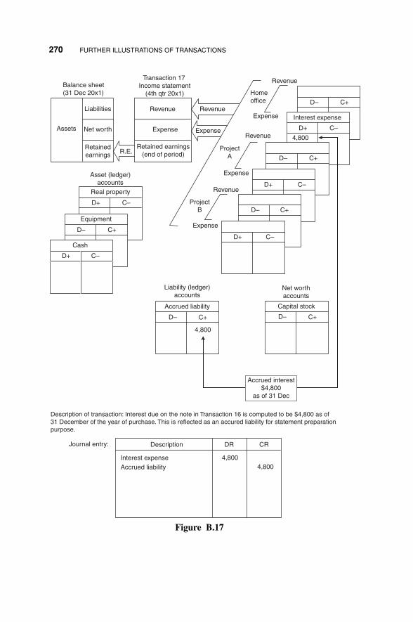
P1: OTA/XYZ P2: ABC



Liabilities Revenue

Revenue

Revenue

Revenue

ProjectA

ProjectB

Homeoffice

Expense

Expense

Expense

Expense Interest expense



Transaction 17


Revenue

Expense

R.E.


D+

4,800

Equipment

Cash


Accrued liability Capital stock

Net worthaccounts

D–

C–

D+ C–

D+ C–C+

D+ C–

D+ C–

D– C+

D– C+

D– C+

D– C+

4,800

D– C+


Interest expense

Accrued liability

CRDR

Description of transaction: Interest due on the note in Transaction 16 is computed to be $4,800 as of31 December of the year of purchase. This is reflected as an accured liability for statement preparationpurpose.

Real property

Assets Net worth

Retainedearnings

4,800

4,800

Accrued interest$4,800

as of 31 Dec

Figure B.17

P1: OTA/XYZ P2: ABC



Liabilities Revenue

Revenue

Revenue

Revenue

ProjectB

ProjectA

Homeoffice

Expense

Expense

Expense

Expense Depreciation expense



Transaction 18


Revenue

Expense

R.E.


D+

7,500

Equipment

Cash


Accumulateddepreciation

Capital stock

Net worthaccounts

D–

C–

D+ C–

D+ C–C+

D+ C–

D+ C–

D– C+

D– C+

D– C+

D– C+

7,500

D– C+


Depreciation expense

Accumulated depreciation

CRDR

Description of transaction: Depreciation on the ditching machine of Transaction 16 as of 31 December is$7,500. An account is maintained to accumulate this expense. This type of account is called a contraaccount. It allows the original value of the asset to be maintained in the “fixed asset–equipment” accountwhile placing the accumulated depreciation in the counterbalancing contra account. The contra accountis considered a liability account.

Real property

Assets Net worth

Retainedearnings

7,500

7,500

Depreciation$7,500

Figure B.18

P1: OTA/XYZ P2: ABC



Liabilities Revenue

Revenue

Revenue

Revenue

ProjectB

ProjectA

Homeoffice

Expense

Expense

Expense

Expense

Interest income



Transaction 19


Revenue

Expense

R.E.


D+

4,000

Equipment

Accrued interestreceivable



Net worthaccounts

D+

C–

D+ C–

D+ C–C–

D+ C–

D+

4,000

C–

D– C+

D– C+

D– C+

D– C+ D– C+


Accrued interest

receivable

Interest income

CRDR

Description of transaction: Interest in the amount of $4,000 has accrued on a certificate of deposit(interest-producing-note) at the bank as of 31 December. This must be reflected in the year-end statementsand is revenue to Apex Construction Company.

Real property

Assets Net worth

Retainedearnings

4,000

4,000

Calculatedinterest oncertificate

ofdeposit$4,000

Figure B.19

P1: OTA/XYZ P2: ABC



Liabilities Revenue

Revenue

Revenue

Revenue

ProjectB

ProjectA

Homeoffice

Expense

Expense

Expense

Expense



Transaction 20


Revenue

Expense

R.E.


D+

Equipment

Cash



Net worthaccounts

4,000

D+

C–

D+ C–

D+ C–

C–

D+ C–

D+ C–

D– C+

D– C+

D– C+

D– C+ D– C+

Accrued interestreceivable

D+ C–


CashAccrued interest receivable

CRDR

4,000

4,000

Description of transaction: Interest in Transaction 19 is paid into construction company account.

Real property

Assets Net worth

Retainedearnings

4,000

$

Figure B.20

P1: OTA/XYZ P2: ABC

JWBT106-APP-C JWBT106-Halpin June 26, 2009 8:56 Printer: Sheridan Books

APPENDIX C

COMPOUND INTEREST TABLES

275



P1: OTA/XYZ P2: ABC


276 COMPOUND INTEREST TABLES

TABLE C.1

0.25% Compound Interest Factors 0.25%

Single Payment Uniform Payment Series

Compound Present Sinking Capital Compound PresentAmount Worth Fund Recovery Amount Worth

n Factor Factor Factor Factor Factor Factor n

Find F Find P Find A Find A Find F Find Pgiven P given F given F given P given A given A

F/P P/F A/F A/P F/A P/A

1 1.00250 0.99751 1.00000 1.00250 1.00000 0.99751 12 1.00501 0.99502 0.49938 0.50188 2.00250 1.99252 23 1.00752 0.99254 0.33250 0.33500 3.00751 2.98506 34 1.01004 0.99006 0.24906 0.25156 4.01503 3.97512 45 1.01256 0.98759 0.19900 0.20150 5.02506 4.96272 5

6 1.01509 0.98513 0.16563 0.16813 6.03763 5.94785 67 1.01763 0.98267 0.14179 0.14429 7.05272 6.93052 78 1.02018 0.98022 0.12391 0.12641 8.07035 7.91074 89 1.02273 0.97778 0.11000 0.11250 9.09053 8.88852 910 1.02528 0.97534 0.09888 0.10138 10.11325 9.86386 10

11 1.02785 0.97291 0.08978 0.09228 11.13854 10.83677 1112 1.03042 0.97048 0.08219 0.08469 12.16638 11.80725 1213 1.03299 0.96806 0.07578 0.07828 13.19680 12.77532 1314 1.03557 0.96565 0.07028 0.07278 14.22979 13.74096 1415 1.03816 0.96324 0.06551 0.06801 15.26537 14.70420 15

16 1.04076 0.96084 0.06134 0.06384 16.30353 15.66504 1617 1.04336 0.95844 0.05766 0.06016 17.34429 16.62348 1718 1.04597 0.95605 0.05438 0.05688 18.38765 17.57953 1819 1.04858 0.95367 0.05146 0.05396 19.43362 18.53320 1920 1.05121 0.95129 0.04882 0.05132 20.48220 19.48449 20

21 1.05383 0.94892 0.04644 0.04894 21.53341 20.43340 2122 1.05647 0.94655 0.04427 0.04677 22.58724 21.37995 2223 1.05911 0.94419 0.04229 0.04479 23.64371 22.32414 2324 1.06176 0.94184 0.04048 0.04298 24.70282 23.26598 2425 1.06441 0.93949 0.03881 0.04131 25.76457 24.20547 25

30 1.07778 0.92783 0.03214 0.03464 31.11331 28.86787 3031 1.08048 0.92552 0.03106 0.03356 32.19109 29.79339 3132 1.08318 0.92321 0.03006 0.03256 33.27157 30.71660 3233 1.08589 0.92091 0.02911 0.03161 34.35475 31.63750 3334 1.08860 0.91861 0.02822 0.03072 35.44064 32.55611 34

35 1.09132 0.91632 0.02738 0.02988 36.52924 33.47243 3536 1.09405 0.91403 0.02658 0.02908 37.62056 34.38647 3642 1.11057 0.90044 0.02261 0.02511 44.22603 39.82300 4248 1.12733 0.88705 0.01963 0.02213 50.93121 45.17869 4860 1.16162 0.86087 0.01547 0.01797 64.64671 55.65236 60

72 1.196948E+00 0.83546 0.01269 0.01519 7.877939E+01 65.81686 72120 1.349354E+00 0.74110 0.00716 0.00966 1.397414E+02 103.56175 120180 1.567432E+00 0.63799 0.00441 0.00691 2.269727E+02 144.80547 180240 1.820755E+00 0.54922 0.00305 0.00555 3.283020E+02 180.31091 240360 2.456842E+00 0.40703 0.00172 0.00422 5.827369E+02 237.18938 360

P1: OTA/XYZ P2: ABC


COMPOUND INTEREST TABLES 277

TABLE C.2







1 1.00500 0.99502 1.00000 1.00500 1.00000 0.99502 12 1.01003 0.99007 0.49875 0.50375 2.00500 1.98510 23 1.01508 0.98515 0.33167 0.33667 3.01502 2.97025 34 1.02015 0.98025 0.24813 0.25313 4.03010 3.95050 45 1.02525 0.97537 0.19801 0.20301 5.05025 4.92587 5

6 1.03038 0.97052 0.16460 0.16960 6.07550 5.89638 67 1.03553 0.96569 0.14073 0.14573 7.10588 6.86207 78 1.04071 0.96089 0.12283 0.12783 8.14141 7.82296 89 1.04591 0.95610 0.10891 0.11391 9.18212 8.77906 910 1.05114 0.95135 0.09777 0.10277 10.22803 9.73041 10

11 1.05640 0.94661 0.08866 0.09366 11.27917 10.67703 1112 1.06168 0.94191 0.08107 0.08607 12.33556 11.61893 1213 1.06699 0.93722 0.07464 0.07964 13.39724 12.55615 1314 1.07232 0.93256 0.06914 0.07414 14.46423 13.48871 1415 1.07768 0.92792 0.06436 0.06936 15.53655 14.41662 15

16 1.08307 0.92330 0.06019 0.06519 16.61423 15.33993 1617 1.08849 0.91871 0.05651 0.06151 17.69730 16.25863 1718 1.09393 0.91414 0.05323 0.05823 18.78579 17.17277 1819 1.09940 0.90959 0.05030 0.05530 19.87972 18.08236 1920 1.10490 0.90506 0.04767 0.05267 20.97912 18.98742 20

21 1.11042 0.90056 0.04528 0.05028 22.08401 19.88798 2122 1.11597 0.89608 0.04311 0.04811 23.19443 20.78406 2223 1.12155 0.89162 0.04113 0.04613 24.31040 21.67568 2324 1.12716 0.88719 0.03932 0.04432 25.43196 22.56287 2425 1.13280 0.88277 0.03765 0.04265 26.55912 23.44564 25

30 1.16140 0.86103 0.03098 0.03598 32.28002 27.79405 3031 1.16721 0.85675 0.02990 0.03490 33.44142 28.65080 3132 1.17304 0.85248 0.02889 0.03389 34.60862 29.50328 3233 1.17891 0.84824 0.02795 0.03295 35.78167 30.35153 3334 1.18480 0.84402 0.02706 0.03206 36.96058 31.19555 34

35 1.19073 0.83982 0.02622 0.03122 38.14538 32.03537 3536 1.19668 0.83564 0.02542 0.03042 39.33610 32.87102 3642 1.23303 0.81101 0.02146 0.02646 46.60654 37.79830 4248 1.27049 0.78710 0.01849 0.02349 54.09783 42.58032 4860 1.34885 0.74137 0.01433 0.01933 69.77003 51.72556 60

72 1.432044E+00 0.69830 0.01157 0.01657 8.640886E+01 60.33951 72120 1.819397E+00 0.54963 0.00610 0.01110 1.638793E+02 90.07345 120180 2.454094E+00 0.40748 0.00344 0.00844 2.908187E+02 118.50351 180240 3.310204E+00 0.30210 0.00216 0.00716 4.620409E+02 139.58077 240360 6.022575E+00 0.16604 0.00100 0.00600 1.004515E+03 166.79161 360

P1: OTA/XYZ P2: ABC



TABLE C.3







1 1.00750 0.99256 1.00000 1.00750 1.00000 0.99256 12 1.01506 0.98517 0.49813 0.50563 2.00750 1.97772 23 1.02267 0.97783 0.33085 0.33835 3.02256 2.95556 34 1.03034 0.97055 0.24721 0.25471 4.04523 3.92611 45 1.03807 0.96333 0.19702 0.20452 5.07556 4.88944 5

6 1.04585 0.95616 0.16357 0.17107 6.11363 5.84560 67 1.05370 0.94904 0.13967 0.14717 7.15948 6.79464 78 1.06160 0.94198 0.12176 0.12926 8.21318 7.73661 89 1.06956 0.93496 0.10782 0.11532 9.27478 8.67158 910 1.07758 0.92800 0.09667 0.10417 10.34434 9.59958 10

11 1.08566 0.92109 0.08755 0.09505 11.42192 10.52067 1112 1.09381 0.91424 0.07995 0.08745 12.50759 11.43491 1213 1.10201 0.90743 0.07352 0.08102 13.60139 12.34235 1314 1.11028 0.90068 0.06801 0.07551 14.70340 13.24302 1415 1.11860 0.89397 0.06324 0.07074 15.81368 14.13699 15

16 1.12699 0.88732 0.05906 0.06656 16.93228 15.02431 1617 1.13544 0.88071 0.05537 0.06287 18.05927 15.90502 1718 1.14396 0.87416 0.05210 0.05960 19.19472 16.77918 1819 1.15254 0.86765 0.04917 0.05667 20.33868 17.64683 1920 1.16118 0.86119 0.04653 0.05403 21.49122 18.50802 20

21 1.16989 0.85478 0.04415 0.05165 22.65240 19.36280 2122 1.17867 0.84842 0.04198 0.04948 23.82230 20.21121 2223 1.18751 0.84210 0.04000 0.04750 25.00096 21.05331 2324 1.19641 0.83583 0.03818 0.04568 26.18847 21.88915 2425 1.20539 0.82961 0.03652 0.04402 27.38488 22.71876 25

30 1.25127 0.79919 0.02985 0.03735 33.50290 26.77508 3031 1.26066 0.79324 0.02877 0.03627 34.75417 27.56832 3132 1.27011 0.78733 0.02777 0.03527 36.01483 28.35565 3233 1.27964 0.78147 0.02682 0.03432 37.28494 29.13712 3334 1.28923 0.77565 0.02593 0.03343 38.56458 29.91278 34

35 1.29890 0.76988 0.02509 0.03259 39.85381 30.68266 3536 1.30865 0.76415 0.02430 0.03180 41.15272 31.44681 3642 1.36865 0.73065 0.02034 0.02784 49.15329 35.91371 4248 1.43141 0.69861 0.01739 0.02489 57.52071 40.18478 4860 1.56568 0.63870 0.01326 0.02076 75.42414 48.17337 60

72 1.712553B+00 0.58392 0.01053 0.01803 9.500703E+01 55.47685 72120 2.451357E+00 0.40794 0.00517 0.01267 1.935143E+02 78.94169 120180 3.838043E+00 0.26055 0.00264 0.01014 3.784058E+02 98.59341 180240 6.009152E+00 0.16641 0.00150 0.00900 6.678869E+02 111.14495 240360 1.473058E+01 0.06789 0.00055 0.00805 1.830743E+03 124.28187 360

P1: OTA/XYZ P2: ABC



TABLE C.4







1 1.01000 0.99010 1.00000 1.01000 1.00000 0.99010 12 1.02010 0.98030 0.49751 0.50751 2.01000 1.97040 23 1.03030 0.97059 0.33002 0.34002 3.03010 2.94099 34 1.04060 0.96098 0.24628 0.25628 4.06040 3.90197 45 1.05101 0.95147 0.19604 0.20604 5.10101 4.85343 5

6 1.06152 0.94205 0.16255 0.17255 6.15202 5.79548 67 1.07214 0.93272 0.13863 0.14863 7.21354 6.72819 78 1.08286 0.92348 0.12069 0.13069 8.28567 7.65168 89 1.09369 0.91434 0.10674 0.11674 9.36853 8.56602 910 1.10462 0.90529 0.09558 0.10558 10.46221 9.47130 10

11 1.11567 0.89632 0.08645 0.09645 11.56683 10.36763 1112 1.12683 0.88745 0.07885 0.08885 12.68250 11.25508 1213 1.13809 0.87866 0.07241 0.08241 13.80933 12.13374 1314 1.14947 0.86996 0.06690 0.07690 14.94742 13.00370 1415 1.16097 0.86135 0.06212 0.07212 16.09690 13.86505 15

16 1.17258 0.85282 0.05794 0.06794 17.25786 14.71787 1617 1.18430 0.84438 0.05426 0.06426 18.43044 15.56225 1718 1.19615 0.83602 0.05098 0.06098 19.61475 16.39827 1819 1.20811 0.82774 0.04805 0.05805 20.81090 17.22601 1920 1.22019 0.81954 0.04542 0.05542 22.01900 18.04555 20

21 1.23239 0.81143 0.04303 0.05303 23.23919 18.85698 2122 1.24472 0.80340 0.04086 0.05086 24.47159 19.66038 2223 1.25716 0.79544 0.03889 0.04889 25.71630 20.45582 2324 1.26973 0.78757 0.03707 0.04707 26.97346 21.24339 2425 1.28243 0.77977 0.03541 0.04541 28.24320 22.02316 25

30 1.34785 0.74192 0.02875 0.03875 34.78489 25.80771 3031 1.36133 0.73458 0.02768 0.03768 36.13274 26.54229 3132 1.37494 0.72730 0.02667 0.03667 37.49407 27.26959 3233 1.38869 0.72010 0.02573 0.03573 38.86901 27.98969 3334 1.40258 0.71297 0.02484 0.03484 40.25770 28.70267 34

35 1.41660 0.70591 0.02400 0.03400 41.66028 29.40858 3536 1.43077 0.69892 0.02321 0.03321 43.07688 30.10751 3642 1.51879 0.65842 0.01928 0.02928 51.87899 34.15811 4248 1.61223 0.62026 0.01633 0.02633 61.22261 37.97396 4860 1.81670 0.55045 0.01224 0.02224 81.66967 44.95504 60

72 2.047099E+00 0.48850 0.00955 0.01955 1.047099E+02 51.15039 72120 3.300387E+00 0.30299 0.00435 0.01435 2.300387E+02 69.70052 120180 5.995802E+00 0.16678 0.00200 0.01200 4.995802E+02 83.32166 180240 1.089255E+01 0.09181 0.00101 0.01101 9.892554E+02 90.81942 240360 3.594964E+01 0.02782 0.00029 0.01029 3.494964E+03 97.21833 360

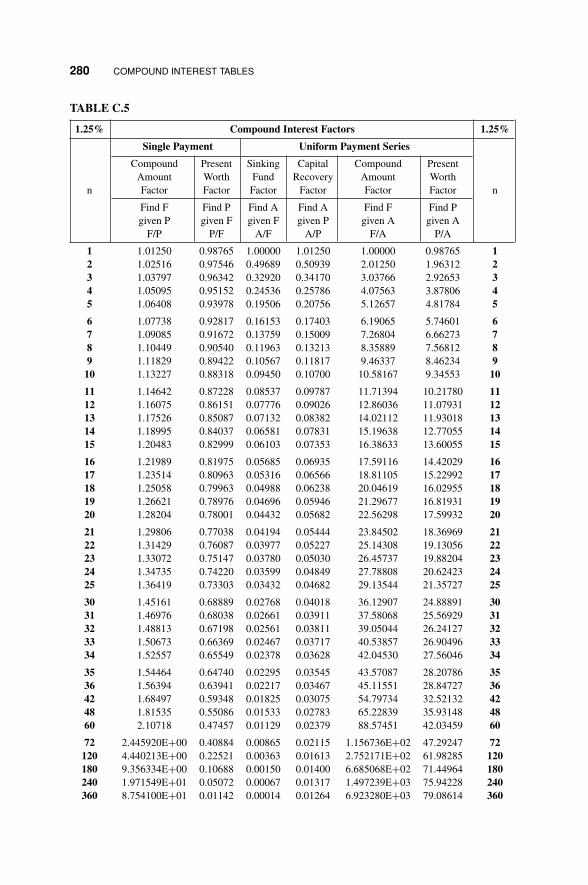
P1: OTA/XYZ P2: ABC



TABLE C.5







1 1.01250 0.98765 1.00000 1.01250 1.00000 0.98765 12 1.02516 0.97546 0.49689 0.50939 2.01250 1.96312 23 1.03797 0.96342 0.32920 0.34170 3.03766 2.92653 34 1.05095 0.95152 0.24536 0.25786 4.07563 3.87806 45 1.06408 0.93978 0.19506 0.20756 5.12657 4.81784 5

6 1.07738 0.92817 0.16153 0.17403 6.19065 5.74601 67 1.09085 0.91672 0.13759 0.15009 7.26804 6.66273 78 1.10449 0.90540 0.11963 0.13213 8.35889 7.56812 89 1.11829 0.89422 0.10567 0.11817 9.46337 8.46234 910 1.13227 0.88318 0.09450 0.10700 10.58167 9.34553 10

11 1.14642 0.87228 0.08537 0.09787 11.71394 10.21780 1112 1.16075 0.86151 0.07776 0.09026 12.86036 11.07931 1213 1.17526 0.85087 0.07132 0.08382 14.02112 11.93018 1314 1.18995 0.84037 0.06581 0.07831 15.19638 12.77055 1415 1.20483 0.82999 0.06103 0.07353 16.38633 13.60055 15

16 1.21989 0.81975 0.05685 0.06935 17.59116 14.42029 1617 1.23514 0.80963 0.05316 0.06566 18.81105 15.22992 1718 1.25058 0.79963 0.04988 0.06238 20.04619 16.02955 1819 1.26621 0.78976 0.04696 0.05946 21.29677 16.81931 1920 1.28204 0.78001 0.04432 0.05682 22.56298 17.59932 20

21 1.29806 0.77038 0.04194 0.05444 23.84502 18.36969 2122 1.31429 0.76087 0.03977 0.05227 25.14308 19.13056 2223 1.33072 0.75147 0.03780 0.05030 26.45737 19.88204 2324 1.34735 0.74220 0.03599 0.04849 27.78808 20.62423 2425 1.36419 0.73303 0.03432 0.04682 29.13544 21.35727 25

30 1.45161 0.68889 0.02768 0.04018 36.12907 24.88891 3031 1.46976 0.68038 0.02661 0.03911 37.58068 25.56929 3132 1.48813 0.67198 0.02561 0.03811 39.05044 26.24127 3233 1.50673 0.66369 0.02467 0.03717 40.53857 26.90496 3334 1.52557 0.65549 0.02378 0.03628 42.04530 27.56046 34

35 1.54464 0.64740 0.02295 0.03545 43.57087 28.20786 3536 1.56394 0.63941 0.02217 0.03467 45.11551 28.84727 3642 1.68497 0.59348 0.01825 0.03075 54.79734 32.52132 4248 1.81535 0.55086 0.01533 0.02783 65.22839 35.93148 4860 2.10718 0.47457 0.01129 0.02379 88.57451 42.03459 60

72 2.445920E+00 0.40884 0.00865 0.02115 1.156736E+02 47.29247 72120 4.440213E+00 0.22521 0.00363 0.01613 2.752171E+02 61.98285 120180 9.356334E+00 0.10688 0.00150 0.01400 6.685068E+02 71.44964 180240 1.971549E+01 0.05072 0.00067 0.01317 1.497239E+03 75.94228 240360 8.754100E+01 0.01142 0.00014 0.01264 6.923280E+03 79.08614 360

P1: OTA/XYZ P2: ABC



TABLE C.6







1 1.01500 0.98522 1.00000 1.01500 1.00000 0.98522 12 1.03023 0.97066 0.49628 0.51128 2.01500 1.95588 23 1.04568 0.95632 0.32838 0.34338 3.04522 2.91220 34 1.06136 0.94218 0.24444 0.25944 4.09090 3.85438 45 1.07728 0.92826 0.19409 0.20909 5.15227 4.78264 5

6 1.09344 0.91454 0.16053 0.17553 6.22955 5.69719 67 1.10984 0.90103 0.13656 0.15156 7.32299 6.59821 78 1.12649 0.88771 0.11858 0.13358 8.43284 7.48593 89 1.14339 0.87459 0.10461 0.11961 9.55933 8.36052 910 1.16054 0.86167 0.09343 0.10843 10.70272 9.22218 10

11 1.17795 0.84893 0.08429 0.09929 11.86326 10.07112 1112 1.19562 0.83639 0.07668 0.09168 13.04121 10.90751 1213 1.21355 0.82403 0.07024 0.08524 14.23683 11.73153 1314 1.23176 0.81185 0.06472 0.07972 15.45038 12.54338 1415 1.25023 0.79985 0.05994 0.07494 16.68214 13.34323 15

16 1.26899 0.78803 0.05577 0.07077 17.93237 14.13126 1617 1.28802 0.77639 0.05208 0.06708 19.20136 14.90765 1718 1.30734 0.76491 0.04881 0.06381 20.48938 15.67256 1819 1.32695 0.75361 0.04588 0.06088 21.79672 16.42617 1920 1.34686 0.74247 0.04325 0.05825 23.12367 17.16864 20

21 1.36706 0.73150 0.04087 0.05587 24.47052 17.90014 2122 1.38756 0.72069 0.03870 0.05370 25.83758 18.62082 2223 1.40838 0.71004 0.03673 0.05173 27.22514 19.33086 2324 1.42950 0.69954 0.03492 0.04992 28.63352 20.03041 2425 1.45095 0.68921 0.03326 0.04826 30.06302 20.71961 25

30 1.56308 0.63976 0.02664 0.04164 37.53868 24.01584 3031 1.58653 0.63031 0.02557 0.04057 39.10176 24.64615 3132 1.61032 0.62099 0.02458 0.03958 40.68829 25.26714 3233 1.63448 0.61182 0.02364 0.03864 42.29861 25.87895 3334 1.65900 0.60277 0.02276 0.03776 43.93309 26.48173 34

35 1.68388 0.59387 0.02193 0.03693 45.59209 27.07559 3536 1.70914 0.58509 0.02115 0.03615 47.27597 27.66068 3642 1.86885 0.53509 0.01726 0.03226 57.92314 30.99405 4248 2.04348 0.48936 0.01437 0.02937 69.56522 34.04255 4860 2.44322 0.40930 0.01039 0.02539 96.21465 39.38027 60

72 2.921158E+00 0.34233 0.00781 0.02281 1.280772E+02 43.84467 72120 5.969323E+00 0.16752 0.00302 0.01802 3.312882E+02 55.49845 120180 1.458437E+01 0.06857 0.00110 0.01610 9.056245E+02 62.09556 180240 3.563282E+01 0.02806 0.00043 0.01543 2.308854E+03 64.79573 240360 2.127038E+02 0.00470 0.00007 0.01507 1.411359E+04 66.35324 360

P1: OTA/XYZ P2: ABC



TABLE C.7







1 1.01750 0.98280 1.00000 1.01750 1.00000 0.98280 12 1.03531 0.96590 0.49566 0.51316 2.01750 1.94870 23 1.05342 0.94929 0.32757 0.34507 3.05281 2.89798 34 1.07186 0.93296 0.24353 0.26103 4.10623 3.83094 45 1.09062 0.91691 0.19312 0.21062 5.17809 4.74786 5

6 1.10970 0.90114 0.15952 0.17702 6.26871 5.64900 67 1.12912 0.88564 0.13553 0.15303 7.37841 6.53464 78 1.14888 0.87041 0.11754 0.13504 8.50753 7.40505 89 1.16899 0.85544 0.10356 0.12106 9.65641 8.26049 910 1.18944 0.84073 0.09238 0.10988 10.82540 9.10122 10

11 1.21026 0.82627 0.08323 0.10073 12.01484 9.92749 1112 1.23144 0.81206 0.07561 0.09311 13.22510 10.73955 1213 1.25299 0.79809 0.06917 0.08667 14.45654 11.53764 1314 1.27492 0.78436 0.06366 0.08116 15.70953 12.32201 1415 1.29723 0.77087 0.05888 0.07638 16.98445 13.09288 15

16 1.31993 0.75762 0.05470 0.07220 18.28168 13.85050 1617 1.34303 0.74459 0.05102 0.06852 19.60161 14.59508 1718 1.36653 0.73178 0.04774 0.06524 20.94463 15.32686 1819 1.39045 0.71919 0.04482 0.06232 22.31117 16.04606 1920 1.41478 0.70682 0.04219 0.05969 23.70161 16.75288 20

21 1.43954 0.69467 0.03981 0.05731 25.11639 17.44755 2122 1.46473 0.68272 0.03766 0.05516 26.55593 18.13027 2223 1.49036 0.67098 0.03569 0.05319 28.02065 18.80125 2324 1.51644 0.65944 0.03389 0.05139 29.51102 19.46069 2425 1.54298 0.64810 0.03223 0.04973 31.02746 20.10878 25

30 1.68280 0.59425 0.02563 0.04313 39.01715 23.18585 3031 1.71225 0.58403 0.02457 0.04207 40.69995 23.76988 3132 1.74221 0.57398 0.02358 0.04108 42.41220 24.34386 3233 1.77270 0.56411 0.02265 0.04015 44.15441 24.90797 3334 1.80372 0.55441 0.02177 0.03927 45.92712 25.46238 34

35 1.83529 0.54487 0.02095 0.03845 47.73084 26.00725 3536 1.86741 0.53550 0.02018 0.03768 49.56613 26.54275 3642 2.07227 0.48256 0.01632 0.03382 61.27236 29.56780 4248 2.29960 0.43486 0.01347 0.03097 74.26278 32.29380 4860 2.83182 0.35313 0.00955 0.02705 104.67522 36.96399 60

72 3.487210E+00 0.28676 0.00704 0.02454 1.421263E+02 40.75645 72120 8.019183E+00 0.12470 0.00249 0.01999 4.010962E+02 50.01709 120180 2.270885E+01 0.04404 0.00081 0.01831 1.240506E+03 54.62653 180240 6.430730E+01 0.01555 0.00028 0.01778 3.617560E+03 56.25427 240360 5.156921E+02 0.00194 0.00003 0.01753 2.941097E+04 57.03205 360

P1: OTA/XYZ P2: ABC



TABLE C.8







1 1.02000 0.98039 1.00000 1.02000 1.00000 0.98039 12 1.04040 0.96117 0.49505 0.51505 2.02000 1.94156 23 1.06121 0.94232 0.32675 0.34675 3.06040 2.88388 34 1.08243 0.92385 0.24262 0.26262 4.12161 3.80773 45 1.10408 0.90573 0.19216 0.21216 5.20404 4.71346 5

6 1.12616 0.88797 0.15853 0.17853 6.30812 5.60143 67 1.14869 0.87056 0.13451 0.15451 7.43428 6.47199 78 1.17166 0.85349 0.11651 0.13651 8.58297 7.32548 89 1.19509 0.83676 0.10252 0.12252 9.75463 8.16224 910 1.21899 0.82035 0.09133 0.11133 10.94972 8.98259 10

;11 1.24337 0.80426 0.08218 0.10218 12.16872 9.78685 1112 1.26824 0.78849 0.07456 0.09456 13.41209 10.57534 1213 1.29361 0.77303 0.06812 0.08812 14.68033 11.34837 1314 1.31948 0.75788 0.06260 0.08260 15.97394 12.10625 1415 1.34587 0.74301 0.05783 0.07783 17.29342 12.84926 15

16 1.37279 0.72845 0.05365 0.07365 18.63929 13.57771 1617 1.40024 0.71416 0.04997 0.06997 20.01207 14.29187 1718 1.42825 0.70016 0.04670 0.06670 21.41231 14.99203 1819 1.45681 0.68643 0.04378 0.06378 22.84056 15.67846 1920 1.48595 0.67297 0.04116 0.06116 24.29737 16.35143 20

21 1.51567 0.65978 0.03878 0.05878 25.78332 17.01121 2122 1.54598 0.64684 0.03663 0.05663 27.29898 17.65805 2223 1.57690 0.63416 0.03467 0.05467 28.84496 18.29220 2324 1.60844 0.62172 0.03287 0.05287 30.42186 18.91393 2425 1.64061 0.60953 0.03122 0.05122 32.03030 19.52346 25

30 1.81136 0.55207 0.02465 0.04465 40.56808 22.39646 3031 1.84759 0.54125 0.02360 0.04360 42.37944 22.93770 3132 1.88454 0.53063 0.02261 0.04261 44.22703 23.46833 3233 1.92223 0.52023 0.02169 0.04169 46.11157 23.98856 3334 1.96068 0.51003 0.02082 0.04082 48.03380 24.49859 34

35 1.99989 0.50003 0.02000 0.04000 49.99448 24.99862 3536 2.03989 0.49022 0.01923 0.03923 51.99437 25.48884 3642 2.29724 0.43530 0.01542 0.03542 64.86222 28.23479 4248 2.58707 0.38654 0.01260 0.03260 79.35352 30.67312 4860 3.28103 0.30478 0.00877 0.02877 114.05154 34.76089 60

72 4.161140E+00 0.24032 0.00633 0.02633 1.580570E+02 37.98406 72120 1.076516E+01 0.09289 0.00205 0.02205 4.882582E+02 45.35539 120180 3.532083E+01 0.02831 0.00058 0.02058 1.716042 E+03 48.58440 180240 1.158887E+02 0.00863 0.00017 0.02017 5.744437E+03 49.56855 240360 1.247561E+03 0.00080 0.00002 0.02002 6.232806E+04 49.95992 360

P1: OTA/XYZ P2: ABC



TABLE C.9







1 1.02500 0.97561 1.00000 1.02500 1.00000 0.97561 12 1.05063 0.95181 0.49383 0.51883 2.02500 1.92742 23 1.07689 0.92860 0.32514 0.35014 3.07563 2.85602 34 1.10381 0.90595 0.24082 0.26582 4.15252 3.76197 45 1.13141 0.88385 0.19025 0.21525 5.25633 4.64583 5

6 1.15969 0.86230 0.15655 0.18155 6.38774 5.50813 67 1.18869 0.84127 0.13250 0.15750 7.54743 6.34939 78 1.21840 0.82075 0.11447 0.13947 8.73612 7.17014 89 1.24886 0.80073 0.10046 0.12546 9.95452 7.97087 910 1.28008 0.78120 0.08926 0.11426 11.20338 8.75206 10

11 1.31209 0.76214 0.08011 0.10511 12.48347 9.51421 1112 1.34489 0.74356 0.07249 0.09749 13.79555 10.25776 1213 1.37851 0.72542 0.06605 0.09105 15.14044 10.98318 1314 1.41297 0.70773 0.06054 0.08554 16.51895 11.69091 1415 1.44830 0.69047 0.05577 0.08077 17.93193 12.38138 15

16 1.48451 0.67362 0.05160 0.07660 19.38022 13.05500 1617 1.52162 0.65720 0.04793 0.07293 20.86473 13.71220 1718 1.55966 0.64117 0.04467 0.06967 22.38635 14.35336 1819 1.59865 0.62553 0.04176 0.06676 23.94601 14.97889 1920 1.63862 0.61027 0.03915 0.06415 25.54466 15.58916 20

21 1.67958 0.59539 0.03679 0.06179 27.18327 16.18455 2122 1.72157 0.58086 0.03465 0.05965 28.86286 16.76541 2223 1.76461 0.56670 0.03270 0.05770 30.58443 17.33211 2324 1.80873 0.55288 0.03091 0.05591 32.34904 17.88499 2425 1.85394 0.53939 0.02928 0.05428 34.15776 18.42438 25

30 2.09757 0.47674 0.02278 0.04778 43.90270 20.93029 3031 2.15001 0.46511 0.02174 0.04674 46.00027 21.39541 3132 2.20376 0.45377 0.02077 0.04577 48.15028 21.84918 3233 2.25885 0.44270 0.01986 0.04486 50.35403 22.29188 3334 2.31532 0.43191 0.01901 0.04401 52.61289 22.72379 34

35 2.37321 0.42137 0.01821 0.04321 54.92821 23.14516 3536 2.43254 0.41109 0.01745 0.04245 57.30141 23.55625 3642 2.82100 0.35448 0.01373 0.03873 72.83981 25.82061 4248 3.27149 0.30567 0.01101 0.03601 90.85958 27.77315 4860 4.39979 0.22728 0.00735 0.03235 135.99159 30.90866 60

72 5.917228E+00 0.16900 0.00508 0.03008 1.966891E+02 33.24008 72120 1.935815E+01 0.05166 0.00136 0.02636 7.343260E+02 37.93369 120180 8.517179E+01 0.01174 0.00030 0.02530 3.366872E+03 39.53036 180240 3.747380E+02 0.00267 0.00007 0.02507 1.494952E+04 39.89326 240360 7.254234E+03 0.00014 0.00000 0.02500 2.901293E+05 39.99449 360

P1: OTA/XYZ P2: ABC



TABLE C.10







1 1.03000 0.97087 1.00000 1.03000 1.00000 0.97087 12 1.06090 0.94260 0.49261 0.52261 2.03000 1.91347 23 1.09273 0.91514 0.32353 0.35353 3.09090 2.82861 34 1.12551 0.88849 0.23903 0.26903 4.18363 3.71710 45 1.15927 0.86261 0.18835 0.21835 5.30914 4.57971 5

6 1.19405 0.83748 0.15460 0.18460 6.46841 5.41719 67 1.22987 0.81309 0.13051 0.16051 7.66246 6.23028 78 1.26677 0.78941 0.11246 0.14246 8.89234 7.01969 89 1.30477 0.76642 0.09843 0.12843 10.15911 7.78611 910 1.34392 0.74409 0.08723 0.11723 11.46388 8.53020 10

11 1.38423 0.72242 0.07808 0.10808 12.80780 9.25262 1112 1.42576 0.70138 0.07046 0.10046 14.19203 9.95400 1213 1.46853 0.68095 0.06403 0.09403 15.61779 10.63496 1314 1.51259 0.66112 0.05853 0.08853 17.08632 11.29607 1415 1.55797 0.64186 0.05377 0.08377 18.59891 11.93794 15

16 1.60471 0.62317 0.04961 0.07961 20.15688 12.56110 1617 1.65285 0.60502 0.04595 0.07595 21.76159 13.16612 1718 1.70243 0.58739 0.04271 0.07271 23.41444 13.75351 1819 1.75351 0.57029 0.03981 0.06981 25.11687 14.32380 1920 1.80611 0.55368 0.03722 0.06722 26.87037 14.87747 20

21 1.86029 0.53755 0.03487 0.06487 28.67649 15.41502 2122 1.91610 0.52189 0.03275 0.06275 30.53678 15.93692 2223 1.97359 0.50669 0.03081 0.06081 32.45288 16.44361 2324 2.03279 0.49193 0.02905 0.05905 34.42647 16.93554 2425 2.09378 0.47761 0.02743 0.05743 36.45926 17.41315 25

30 2.42726 0.41199 0.02102 0.05102 47.57542 19.60044 3031 2.50008 0.39999 0.02000 0.05000 50.00268 20.00043 3132 2.57508 0.38834 0.01905 0.04905 52.50276 20.38877 3233 2.65234 0.37703 0.01816 0.04816 55.07784 20.76579 3334 2.73191 0.36604 0.01732 0.04732 57.73018 21.13184 34

35 2.81386 0.35538 0.01654 0.04654 60.46208 21.48722 3536 2.89828 0.34503 0.01580 0.04580 63.27594 21.83225 3642 3.46070 0.28896 0.01219 0.04219 82.02320 23.70136 4248 4.13225 0.24200 0.00958 0.03958 104.40840 25.26671 4860 5.89160 0.16973 0.00613 0.03613 163.05344 27.67556 60

72 8.400017E+00 0.11905 0.00405 0.03405 2.466672E+02 29.36509 72120 3.471099E+01 0.02881 0.00089 0.03089 1.123700E+03 32.37302 120180 2.045034E+02 0.00489 0.00015 0.03015 6.783445E+03 33.17034 180240 1.204853E+03 0.00083 0.00002 0.03002 4.012842E+04 33.30567 240360 4.182162E+04 0.00002 0.00000 0.03000 1.394021E+06 33.33254 360

P1: OTA/XYZ P2: ABC



TABLE C.11







1 1.04000 0.96154 1.00000 1.04000 1.00000 0.96154 12 1.08160 0.92456 0.49020 0.53020 2.04000 1.88609 23 1.12486 0.88900 0.32035 0.36035 3.12160 2.77509 34 1.16986 0.85480 0.23549 0.27549 4.24646 3.62990 45 1.21665 0.82193 0.18463 0.22463 5.41632 4.45182 5

6 1.26532 0.79031 0.15076 0.19076 6.63298 5.24214 67 1.31593 0.75992 0.12661 0.16661 7.89829 6.00205 78 1.36857 0.73069 0.10853 0.14853 9.21423 6.73274 89 1.42331 0.70259 0.09449 0.13449 10.58280 7.43533 910 1.48024 0.67556 0.08329 0.12329 12.00611 8.11090 10

11 1.53945 0.64958 0.07415 0.11415 13.48635 8.76048 1112 1.60103 0.62460 0.06655 0.10655 15.02581 9.38507 1213 1.66507 0.60057 0.06014 0.10014 16.62684 9.98565 1314 1.73168 0.57748 0.05467 0.09467 18.29191 10.56312 1415 1.80094 0.55526 0.04994 0.08994 20.02359 11.11839 15

16 1.87298 0.53391 0.04582 0.08582 21.82453 11.65230 1617 1.94790 0.51337 0.04220 0.08220 23.69751 12.16567 1718 2.02582 0.49363 0.03899 0.07899 25.64541 12.65930 1819 2.10685 0.47464 0.03614 0.07614 27.67123 13.13394 1920 2.19112 0.45639 0.03358 0.07358 29.77808 13.59033 20

21 2.27877 0.43883 0.03128 0.07128 31.96920 14.02916 2122 2.36992 0.42196 0.02920 0.06920 34.24797 14.45112 2223 2.46472 0.40573 0.02731 0.06731 36.61789 14.85684 2324 2.56330 0.39012 0.02559 0.06559 39.08260 15.24696 2425 2.66584 0.37512 0.02401 0.06401 41.64591 15.62208 25

30 3.24340 0.30832 0.01783 0.05783 56.08494 17.29203 3031 3.37313 0.29646 0.01686 0.05686 59.32834 17.58849 3132 3.50806 0.28506 0.01595 0.05595 62.70147 17.87355 3233 3.64838 0.27409 0.01510 0.05510 66.20953 18.14765 3334 3.79432 0.26355 0.01431 0.05431 69.85791 18.41120 34

35 3.94609 0.25342 0.01358 0.05358 73.65222 18.66461 3536 4.10393 0.24367 0.01289 0.05289 77.59831 18.90828 3642 5.19278 0.19257 0.00954 0.04954 104.81960 20.18563 4248 6.57053 0.15219 0.00718 0.04718 139.26321 21.19513 4860 10.51963 0.09506 0.00420 0.04420 237.99069 22.62349 60

72 1.684226E+01 0.05937 0.00252 0.04252 3.960566E+02 23.51564 72120 1.106626E+02 0.00904 0.00036 0.04036 2.741564E+03 24.77409 120180 1.164129E+03 0.00086 0.00003 0.04003 2.907822E+04 24.97852 180240 1.224620E+04 0.00008 0.00000 0.04000 3.061301E+05 24.99796 240360 1.355196E+06 0.00000 0.00000 0.04000 3.387988E+07 24.99998 360

P1: OTA/XYZ P2: ABC



TABLE C.12







1 1.05000 0.95238 1.00000 1.05000 1.00000 0.95238 12 1.10250 0.90703 0.48780 0.53780 2.05000 1.85941 23 1.15763 0.86384 0.31721 0.36721 3.15250 2.72325 34 1.21551 0.82270 0.23201 0.28201 4.31013 3.54595 45 1.27628 0.78353 0.18097 0.23097 5.52563 4.32948 5

6 1.34010 0.74622 0.14702 0.19702 6.80191 5.07569 67 1.40710 0.71068 0.12282 0.17282 8.14201 5.78637 78 1.47746 0.67684 0.10472 0.15472 9.54911 6.46321 89 1.55133 0.64461 0.09069 0.14069 11.02656 7.10782 910 1.62889 0.61391 0.07950 0.12950 12.57789 7.72173 10

11 1.71034 0.58468 0.07039 0.12039 14.20679 8.30641 1112 1.79586 0.55684 0.06283 0.11283 15.91713 8.86325 1213 1.88565 0.53032 0.05646 0.10646 17.71298 9.39357 1314 1.97993 0.50507 0.05102 0.10102 19.59863 9.89864 1415 2.07893 0.48102 0.04634 0.09634 21.57856 10.37966 15

16 2.18287 0.45811 0.04227 0.09227 23.65749 10.83777 1617 2.29202 0.43630 0.03870 0.08870 25.84037 11.27407 1718 2.40662 0.41552 0.03555 0.08555 28.13238 11.68959 1819 2.52695 0.39573 0.03275 0.08275 30.53900 12.08532 1920 2.65330 0.37689 0.03024 0.08024 33.06595 12.46221 20

21 2.78596 0.35894 0.02800 0.07800 35.71925 12.82115 2122 2.92526 0.34185 0.02597 0.07597 38.50521 13.16300 2223 3.07152 0.32557 0.02414 0.07414 41.43048 13.48857 2324 3.22510 0.31007 0.02247 0.07247 44.50200 13.79864 2425 3.38635 0.29530 0.02095 0.07095 47.72710 14.09394 25

30 4.32194 0.23138 0.01505 0.06505 66.43885 15.37245 3031 4.53804 0.22036 0.01413 0.06413 70.76079 15.59281 3132 4.76494 0.20987 0.01328 0.06328 75.29883 15.80268 3233 5.00319 0.19987 0.01249 0.06249 80.06377 16.00255 3334 5.25335 0.19035 0.01176 0.06176 85.06696 16.19290 34

35 5.51602 0.18129 0.01107 0.06107 90.32031 16.37419 3536 5.79182 0.17266 0.01043 0.06043 95.83632 16.54685 3642 7.76159 0.12884 0.00739 0.05739 135.23175 17.42321 4248 10.40127 0.09614 0.00532 0.05532 188.02539 18.07716 4860 18.67919 0.05354 0.00283 0.05283 353.58372 18.92929 60

72 3.354513E+01 0.02981 0.00154 0.05154 6.509027E+02 19.40379 72120 3.489120E+02 0.00287 0.00014 0.05014 6.958240E+03 19.94268 120180 6.517392E+03 0.00015 0.00001 0.05001 1.303278E+05 19.99693 180240 1.217396E+05 0.00001 0.00000 0.05000 2.434771E+06 19.99984 240360 4.247640E+07 0.00000 0.00000 0.05000 8.495279E+08 20.00000 360

P1: OTA/XYZ P2: ABC



TABLE C.13







1 1.06000 0.94340 1.00000 1.06000 1.00000 0.94340 12 1.12360 0.89000 0.48544 0.54544 2.06000 1.83339 23 1.19102 0.83962 0.31411 0.37411 3.18360 2.67301 34 1.26248 0.79209 0.22859 0.28859 4.37462 3.46511 45 1.33823 0.74726 0.17740 0.23740 5.63709 4.21236 5

6 1.41852 0.70496 0.14336 0.20336 6.97532 4.91732 67 1.50363 0.66506 0.11914 0.17914 8.39384 5.58238 78 1.59385 0.62741 0.10104 0.16104 9.89747 6.20979 89 1.68948 0.59190 0.08702 0.14702 11.49132 6.80169 910 1.79085 0.55839 0.07587 0.13587 13.18079 7.36009 10

11 1.89830 0.52679 0.06679 0.12679 14.97164 7.88687 1112 2.01220 0.49697 0.05928 0.11928 16.86994 8.38384 1213 2.13293 0.46884 0.05296 0.11296 18.88214 8.85268 1314 2.26090 0.44230 0.04758 0.10758 21.01507 9.29498 1415 2.39656 0.41727 0.04296 0.10296 23.27597 9.71225 15

16 2.54035 0.39365 0.03895 0.09895 25.67253 10.10590 1617 2.69277 0.37136 0.03544 0.09544 28.21288 10.47726 1718 2.85434 0.35034 0.03236 0.09236 30.90565 10.82760 1819 3.02560 0.33051 0.02962 0.08962 33.75999 11.15812 1920 3.20714 0.31180 0.02718 0.08718 36.78559 11.46992 20

21 3.39956 0.29416 0.02500 0.08500 39.99273 11.76408 2122 3.60354 0.27751 0.02305 0.08305 43.39229 12.04158 2223 3.81975 0.26180 0.02128 0.08128 46.99583 12.30338 2324 4.04893 0.24698 0.01968 0.07968 50.81558 12.55036 2425 4.29187 0.23300 0.01823 0.07823 54.86451 12.78336 25

30 5.74349 0.17411 0.01265 0.07265 79.05819 13.76483 3031 6.08810 0.16425 0.01179 0.07179 84.80168 13.92909 3132 6.45339 0.15496 0.01100 0.07100 90.88978 14.08404 3233 6.84059 0.14619 0.01027 0.07027 97.34316 14.23023 3334 7.25103 0.13791 0.00960 0.06960 104.18375 14.36814 34

35 7.68609 0.13011 0.00897 0.06897 111.43478 14.49825 3536 8.14725 0.12274 0.00839 0.06839 119.12087 14.62099 3642 11.55703 0.08653 0.00568 0.06568 175.95054 15.22454 4248 16.39387 0.06100 0.00390 0.06390 256.56453 15.65003 4860 32.98769 0.03031 0.00188 0.06188 533.12818 16.16143 60

72 6.637772E+01 0.01507 0.00092 0.06092 1.089629E+03 16.41558 72120 1.088188E+03 0.00092 0.00006 0.06006 1.811980E+04 16.65135 120180 3.589680E+04 0.00003 0.00000 0.06000 5.982634E+05 16.66620 180240 1.184153E+06 0.00000 0.00000 0.06000 1.973586E+07 16.66665 240360 1.288580E+09 0.00000 0.00000 0.06000 2.147634E+10 16.66667 360

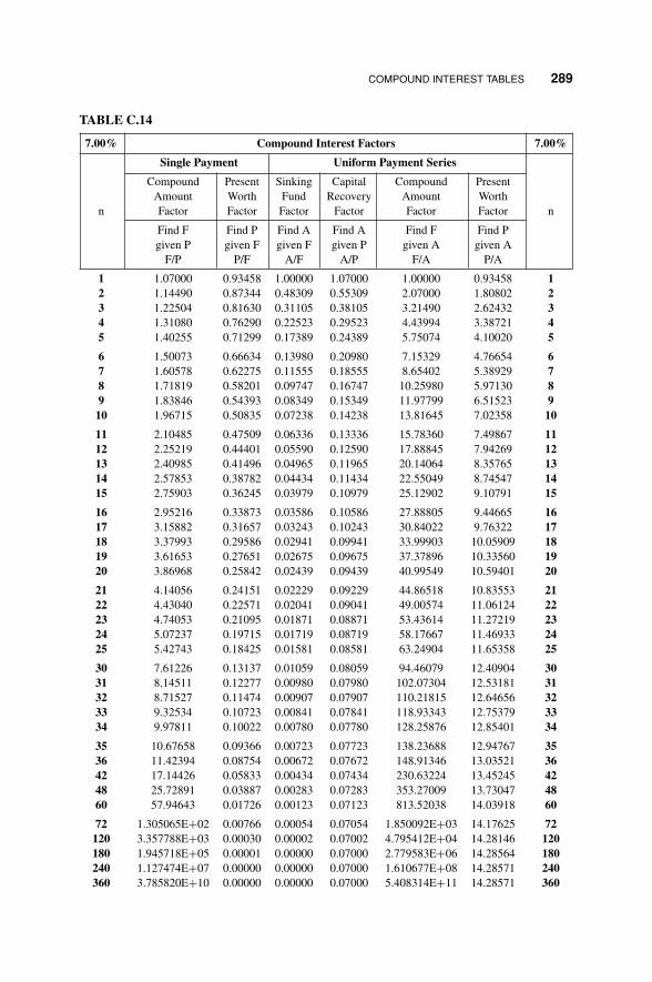
P1: OTA/XYZ P2: ABC



TABLE C.14







1 1.07000 0.93458 1.00000 1.07000 1.00000 0.93458 12 1.14490 0.87344 0.48309 0.55309 2.07000 1.80802 23 1.22504 0.81630 0.31105 0.38105 3.21490 2.62432 34 1.31080 0.76290 0.22523 0.29523 4.43994 3.38721 45 1.40255 0.71299 0.17389 0.24389 5.75074 4.10020 5

6 1.50073 0.66634 0.13980 0.20980 7.15329 4.76654 67 1.60578 0.62275 0.11555 0.18555 8.65402 5.38929 78 1.71819 0.58201 0.09747 0.16747 10.25980 5.97130 89 1.83846 0.54393 0.08349 0.15349 11.97799 6.51523 910 1.96715 0.50835 0.07238 0.14238 13.81645 7.02358 10

11 2.10485 0.47509 0.06336 0.13336 15.78360 7.49867 1112 2.25219 0.44401 0.05590 0.12590 17.88845 7.94269 1213 2.40985 0.41496 0.04965 0.11965 20.14064 8.35765 1314 2.57853 0.38782 0.04434 0.11434 22.55049 8.74547 1415 2.75903 0.36245 0.03979 0.10979 25.12902 9.10791 15

16 2.95216 0.33873 0.03586 0.10586 27.88805 9.44665 1617 3.15882 0.31657 0.03243 0.10243 30.84022 9.76322 1718 3.37993 0.29586 0.02941 0.09941 33.99903 10.05909 1819 3.61653 0.27651 0.02675 0.09675 37.37896 10.33560 1920 3.86968 0.25842 0.02439 0.09439 40.99549 10.59401 20

21 4.14056 0.24151 0.02229 0.09229 44.86518 10.83553 2122 4.43040 0.22571 0.02041 0.09041 49.00574 11.06124 2223 4.74053 0.21095 0.01871 0.08871 53.43614 11.27219 2324 5.07237 0.19715 0.01719 0.08719 58.17667 11.46933 2425 5.42743 0.18425 0.01581 0.08581 63.24904 11.65358 25

30 7.61226 0.13137 0.01059 0.08059 94.46079 12.40904 3031 8.14511 0.12277 0.00980 0.07980 102.07304 12.53181 3132 8.71527 0.11474 0.00907 0.07907 110.21815 12.64656 3233 9.32534 0.10723 0.00841 0.07841 118.93343 12.75379 3334 9.97811 0.10022 0.00780 0.07780 128.25876 12.85401 34

35 10.67658 0.09366 0.00723 0.07723 138.23688 12.94767 3536 11.42394 0.08754 0.00672 0.07672 148.91346 13.03521 3642 17.14426 0.05833 0.00434 0.07434 230.63224 13.45245 4248 25.72891 0.03887 0.00283 0.07283 353.27009 13.73047 4860 57.94643 0.01726 0.00123 0.07123 813.52038 14.03918 60

72 1.305065E+02 0.00766 0.00054 0.07054 1.850092E+03 14.17625 72120 3.357788E+03 0.00030 0.00002 0.07002 4.795412E+04 14.28146 120180 1.945718E+05 0.00001 0.00000 0.07000 2.779583E+06 14.28564 180240 1.127474E+07 0.00000 0.00000 0.07000 1.610677E+08 14.28571 240360 3.785820E+10 0.00000 0.00000 0.07000 5.408314E+11 14.28571 360

P1: OTA/XYZ P2: ABC



TABLE C.15







1 1.08000 0.92593 1.00000 1.08000 1.00000 0.92593 12 1.16640 0.85734 0.48077 0.56077 2.08000 1.78326 23 1.25971 0.79383 0.30803 0.38803 3.24640 2.57710 34 1.36049 0.73503 0.22192 0.30192 4.50611 3.31213 45 1.46933 0.68058 0.17046 0.25046 5.86660 3.99271 5

6 1.58687 0.63017 0.13632 0.21632 7.33593 4.62288 67 1.71382 0.58349 0.11207 0.19207 8.92280 5.20637 78 1.85093 0.54027 0.09401 0.17401 10.63663 5.74664 89 1.99900 0.50025 0.08008 0.16008 12.48756 6.24689 910 2.15892 0.46319 0.06903 0.14903 14.48656 6.71008 10

11 2.33164 0.42888 0.06008 0.14008 16.64549 7.13896 1112 2.51817 0.39711 0.05270 0.13270 18.97713 7.53608 1213 2.71962 0.36770 0.04652 0.12652 21.49530 7.90378 1314 2.93719 0.34046 0.04130 0.12130 24.21492 8.24424 1415 3.17217 0.31524 0.03683 0.11683 27.15211 8.55948 15

16 3.42594 0.29189 0.03298 0.11298 30.32428 8.85137 1617 3.70002 0.27027 0.02963 0.10963 33.75023 9.12164 1718 3.99602 0.25025 0.02670 0.10670 37.45024 9.37189 1819 4.31570 0.23171 0.02413 0.10413 41.44626 9.60360 1920 4.66096 0.21455 0.02185 0.10185 45.76196 9.81815 20

21 5.03383 0.19866 0.01983 0.09983 50.42292 10.01680 2122 5.43654 0.18394 0.01803 0.09803 55.45676 10.20074 2223 5.87146 0.17032 0.01642 0.09642 60.89330 10.37106 2324 6.34118 0.15770 0.01498 0.09498 66.76476 10.52876 2425 6.84848 0.14602 0.01368 0.09368 73.10594 10.67478 25

30 10.06266 0.09938 0.00883 0.08883 113.28321 11.25778 3031 10.86767 0.09202 0.00811 0.08811 123.34587 11.34980 3132 11.73708 0.08520 0.00745 0.08745 134.21354 11.43500 3233 12.67605 0.07889 0.00685 0.08685 145.95062 11.51389 3334 13.69013 0.07305 0.00630 0.08630 158.62667 11.58693 34

35 14.78534 0.06763 0.00580 0.08580 172.31680 11.65457 3536 15.96817 0.06262 0.00534 0.08534 187.10215 11.71719 3642 25.33948 0.03946 0.00329 0.08329 304.24352 12.00670 4248 40.21057 0.02487 0.00204 0.08204 490.13216 12.18914 4860 101.25706 0.00988 0.00080 0.08080 1253.21330 12.37655 60

72 2.549825E+02 0.00392 0.00031 0.08031 3.174781E+03 12.45098 72120 1.025299E+04 0.00010 0.00001 0.08001 1.281499E+05 12.49878 120180 1.038188E+06 0.00000 0.00000 0.08000 1.297734E+07 12.49999 180240 1.051239E+08 0.00000 0.00000 0.08000 1.314048E+09 12.50000 240360 1.077834E+12 0.00000 0.00000 0.08000 1.347293E+13 12.50000 360

P1: OTA/XYZ P2: ABC



TABLE C.16







1 1.09000 0.91743 1.00000 1.09000 1.00000 0.91743 12 1.18810 0.84168 0.47847 0.56847 2.09000 1.75911 23 1.29503 0.77218 0.30505 0.39505 3.27810 2.53129 34 1.41158 0.70843 0.21867 0.30867 4.57313 3.23972 45 1.53862 0.64993 0.16709 0.25709 5.98471 3.88965 5

6 1.67710 0.59627 0.13292 0.22292 7.52333 4.48592 67 1.82804 0.54703 0.10869 0.19869 9.20043 5.03295 78 1.99256 0.50187 0.09067 0.18067 11.02847 5.53482 89 2.17189 0.46043 0.07680 0.16680 13.02104 5.99525 910 2.36736 0.42241 0.06582 0.15582 15.19293 6.41766 10

11 2.58043 0.38753 0.05695 0.14695 17.56029 6.80519 1112 2.81266 0.35553 0.04965 0.13965 20.14072 7.16073 1213 3.06580 0.32618 0.04357 0.13357 22.95338 7.48690 1314 3.34173 0.29925 0.03843 0.12843 26.01919 7.78615 1415 3.64248 0.27454 0.03406 0.12406 29.36092 8.06069 15

16 3.97031 0.25187 0.03030 0.12030 33.00340 8.31256 1617 4.32763 0.23107 0.02705 0.11705 36.97370 8.54363 1718 4.71712 0.21199 0.02421 0.11421 41.30134 8.75563 1819 5.14166 0.19449 0.02173 0.11173 46.01846 8.95011 1920 5.60441 0.17843 0.01955 0.10955 51.16012 9.12855 20

21 6.10881 0.16370 0.01762 0.10762 56.76453 9.29224 2122 6.65860 0.15018 0.01590 0.10590 62.87334 9.44243 2223 7.25787 0.13778 0.01438 0.10438 69.53194 9.58021 2324 7.91108 0.12640 0.01302 0.10302 76.78981 9.70661 2425 8.62308 0.11597 0.01181 0.10181 84.70090 9.82258 25

30 13.26768 0.07537 0.00734 0.09734 136.30754 10.27365 3031 14.46177 0.06915 0.00669 0.09669 149.57522 10.34280 3132 15.76333 0.06344 0.00610 0.09610 164.03699 10.40624 3233 17.18203 0.05820 0.00556 0.09556 179.80032 10.46444 3334 18.72841 0.05339 0.00508 0.09508 196.98234 10.51784 34

35 20.41397 0.04899 0.00464 0.09464 215.71075 10.56682 3536 22.25123 0.04494 0.00424 0.09424 236.12472 10.61176 3642 37.31753 0.02680 0.00248 0.09248 403.52813 10.81337 4248 62.58524 0.01598 0.00146 0.09146 684.28041 10.93358 4860 176.03129 0.00568 0.00051 0.09051 1944.79213 11.04799 60

72 4.951170E+02 0.00202 0.00018 0.09018 5.490189E+03 11.08867 72120 3.098702E+04 0.00003 0.00000 0.09000 3.442891E+05 11.11075 120180 5.454684E+06 0.00000 0.00000 0.09000 6.060759E+07 11.11111 180240 9.601951E+08 0.00000 0.00000 0.09000 1.066883E+10 11.11111 240360 2.975358E+13 0.00000 0.00000 0.09000 3.305954E+14 11.11111 360

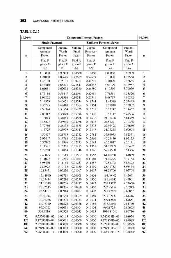
P1: OTA/XYZ P2: ABC



TABLE C.17







1 1.10000 0.90909 1.00000 1.10000 1.00000 0.90909 12 1.21000 0.82645 0.47619 0.57619 2.10000 1.73554 23 1.33100 0.75131 0.30211 0.40211 3.31000 2.48685 34 1.46410 0.68301 0.21547 0.31547 4.64100 3.16987 45 1.61051 0.62092 0.16380 0.26380 6.10510 3.79079 5

6 1.77156 0.56447 0.12961 0.22961 7.71561 4.35526 67 1.94872 0.51316 0.10541 0.20541 9.48717 4.86842 78 2.14359 0.46651 0.08744 0.18744 11.43589 5.33493 89 2.35795 0.42410 0.07364 0.17364 13.57948 5.75902 910 2.59374 0.38554 0.06275 0.16275 15.93742 6.14457 10

11 2.85312 0.35049 0.05396 0.15396 18.53117 6.49506 1112 3.13843 0.31863 0.04676 0.14676 21.38428 6.81369 1213 3.45227 0.28966 0.04078 0.14078 24.52271 7.10336 1314 3.79750 0.26333 0.03575 0.13575 27.97498 7.36669 1415 4.17725 0.23939 0.03147 0.13147 31.77248 7.60608 15

16 4.59497 0.21763 0.02782 0.12782 35.94973 7.82371 1617 5.05447 0.19784 0.02466 0.12466 40.54470 8.02155 1718 5.55992 0.17986 0.02193 0.12193 45.59917 8.20141 1819 6.11591 0.16351 0.01955 0.11955 51.15909 8.36492 1920 6.72750 0.14864 0.01746 0.11746 57.27500 8.51356 20

21 7.40025 0.13513 0.01562 0.11562 64.00250 8.64869 2122 8.14027 0.12285 0.01401 .0.11401 71.40275 8.77154 2223 8.95430 0.11168 0.01257 0.11257 79.54302 8.88322 2324 9.84973 0.10153 0.01130 0.11130 88.49733 8.98474 2425 10.83471 0.09230 0.01017 0.11017 98.34706 9.07704 25

30 17.44940 0.05731 0.00608 0.10608 164.49402 9.42691 3031 19.19434 0.05210 0.00550 0.10550 181.94342 9.47901 3132 21.11378 0.04736 0.00497 0.10497 201.13777 9.52638 3233 23.22515 0.04306 0.00450 0.10450 222.25154 9.56943 3334 25.54767 0.03914 0.00407 0.10407 245.47670 9.60857 34

35 28.10244 0.03558 0.00369 0.10369 271.02437 9.64416 3536 30.91268 0.03235 0.00334 0.10334 299.12681 9.67651 3642 54.76370 0.01826 0.00186 0.10186 537.63699 9.81740 4248 97.01723 0.01031 0.00104 0.10104 960.17234 9.89693 4860 304.48164 0.00328 0.00033 0.10033 3034.81640 9.96716 60

72 9.555938E+02 0.00105 0.00010 0.10010 9.545938E+03 9.98954 72120 9.270907E+04 0.00001 0.00000 0.10000 9.270807E+05 9.99989 120180 2.822821E+07 0.00000 0.00000 0.10000 2.822821E+08 10.00000 180240 8.594971E+09 0.00000 0.00000 0.10000 8.594971E+10 10.00000 240360 7.968318E+14 0.00000 0.00000 0.10000 7.968318E+15 10.00000 360

P1: OTA/XYZ P2: ABC



TABLE C.18







1 1.11000 0.90090 1.00000 1.11000 1.00000 0.90090 12 1.23210 0.81162 0.47393 0.58393 2.11000 1.71252 23 1.36763 0.73119 0.29921 0.40921 3.34210 2.44371 34 1.51807 0.65873 0.21233 0.32233 4.70973 3.10245 45 1.68506 0.59345 0.16057 0.27057 6.22780 3.69590 5

6 1.87041 0.53464 0.12638 0.23638 7.91286 4.23054 67 2.07616 0.48166 0.10222 0.21222 9.78327 4.71220 78 2.30454 0.43393 0.08432 0.19432 11.85943 5.14612 89 2.55804 0.39092 0.07060 0.18060 14.16397 5.53705 910 2.83942 0.35218 0.05980 0.16980 16.72201 5.88923 10

11 3.15176 0.31728 0.05112 0.16112 19.56143 6.20652 1112 3.49845 0.28584 0.04403 0.15403 22.71319 6.49236 1213 3.88328 0.25751 0.03815 0.14815 26.21164 6.74987 1314 4.31044 0.23199 0.03323 0.14323 30.09492 6.98187 1415 4.78459 0.20900 0.02907 0.13907 34.40536 7.19087 15

16 5.31089 0.18829 0.02552 0.13552 39.18995 7.37916 1617 5.89509 0.16963 0.02247 0.13247 44.50084 7.54879 1718 6.54355 0.15282 0.01984 0.12984 50.39594 7.70162 1819 7.26334 0.13768 0.01756 0.12756 56.93949 7.83929 1920 8.06231 0.12403 0.01558 0.12558 64.20283 7.96333 20

21 8.94917 0.11174 0.01384 0.12384 72.26514 8.07507 2122 9.93357 0.10067 0.01231 0.12231 81.21431 8.17574 2223 11.02627 0.09069 0.01097 0.12097 91.14788 8.26643 2324 12.23916 0.08170 0.00979 0.11979 102.17415 8.34814 2425 13.58546 0.07361 0.00874 0.11874 114.41331 8.42174 25

30 22.89230 0.04368 0.00502 0.11502 199.02088 8.69379 3031 25.41045 0.03935 0.00451 0.11451 221.91317 8.73315 3132 28.20560 0.03545 0.00404 0.11404 247.32362 8.76860 3233 31.30821 0.03194 0.00363 0.11363 275.52922 8.80054 3334 34.75212 0.02878 0.00326 0.11326 306.83744 8.82932 34

35 38.57485 0.02592 0.00293 0.11293 341.58955 8.85524 3536 42.81808 0.02335 0.00263 0.11263 380.16441 8.87859 3642 80.08757 0.01249 0.00139 0.11139 718.97790 8.97740 4248 149.79695 0.00668 0.00074 0.11074 1352.69958 9.03022 4860 524.05724 0.00191 0.00021 0.11021 4755.06584 9.07356 60

72 1.833388E+03 0.00055 0.00006 0.11006 1.665808E+04 9.08595 72120 2.746360E+05 0.00000 0.00000 0.11000 2.496682E+06 9.09088 120180 1.439250E+08 0.00000 0.00000 0.11000 1.308409E+09 9.09091 180240 7.542493E+10 0.00000 0.00000 0.11000 6.856812E+11 9.09091 240360 2.071440E+16 0.00000 0.00000 0.11000 1.883127E+17 9.09091 360

P1: OTA/XYZ P2: ABC



TABLE C.19







1 1.12000 0.89286 1.00000 1.12000 1.00000 0.89286 12 1.25440 0.79719 0.47170 0.59170 2.12000 1.69005 23 1.40493 0.71178 0.29635 0.41635 3.37440 2.40183 34 1.57352 0.63552 0.20923 0.32923 4.77933 3.03735 45 1.76234 0.56743 0:15741 0.27741 6.35285 3.60478 5

6 1.97382 0.50663 0.12323 0.24323 8.11519 4.11141 67 2.21068 0.45235 0.09912 0.21912 10.08901 4.56376 78 2.47596 0.40388 0.08130 0.20130 12.29969 4.96764 89 2.77308 0.36061 0.06768 0.18768 14.77566 5.32825 910 3.10585 0.32197 0.05698 0.17698 17.54874 5.65022 10

11 3.47855 0.28748 0.04842 0.16842 20.65458 5.93770 1112 3.89598 0.25668 0.04144 0.16144 24.13313 6.19437 1213 4.36349 0.22917 0.03568 0.15568 28.02911 6.42355 1314 4.88711 0.20462 0.03087 0.15087 32.39260 6.62817 1415 5.47357 0.18270 0.02682 0.14682 37.27971 6.81086 15

16 6.13039 0.16312 0.02339 0.14339 42.75328 6.97399 1617 6.86604 0.14564 0.02046 0.14046 48.88367 7.11963 1718 7.68997 0.13004 0.01794 0.13794 55.74971 7.24967 1819 8.61276 0.11611 0.01576 0.13576 63.43968 7.36578 1920 9.64629 0.10367 0.01388 0.13388 72.05244 7.46944 20

21 10.80385 0.09256 0.01224 0.13224 81.69874 7.56200 2122 12.10031 0.08264 0.01081 0.13081 92.50258 7.64465 2223 13.55235 0.07379 0.00956 0.12956 104.60289 7.71843 2324 15.17863 0.06588 0.00846 0.12846 118.15524 7.78432 2425 17.00006 0.05882 0.00750 0.12750 133.33387 7.84314 25

30 29.95992 0.03338 0.00414 0.12414 241.33268 8.05518 3031 33.55511 0.02980 0.00369 0.12369 271.29261 8.08499 3132 37:58173 0.02661 0.00328 0.12328 304.84772 8.11159 3233 42.09153 0.02376 0.00292 0.12292 342.42945 8.13535 3334 47.14252 0.02121 0.00260 0.12260 384.52098 8.15656 34

35 52.79962 0.01894 0.00232 0.12232 431.66350 8.17550 3536 59.13557 0.01691 0.00206 0.12206 484.46312 8.19241 3642 116.72314 0.00857 0.00104 0.12104 964.35948 8.26194 4248 230.39078 0.00434 0.00052 0.12052 1911.58980 8.29716 4860 897.59693 0.00111 0.00013 0.12013 7471.64111 8.32405 60

72 3.497016E+03 0.00029 0.00003 0.12003 2.913347E+04 8.33095 72120 8.056803E+05 0.00000 0.00000 0.12000 6.713994E+06 8.33332 120180 7.231761E+08 0.00000 0.00000 0.12000 6.026468E+09 8.33333 180240 6.491207E+11 0.00000 0.00000 0.12000 5.409339E+12 8.33333 240360 5.229837E+17 0.00000 0.00000 0.12000 4.358198E+18 8.33333 360

P1: OTA/XYZ P2: ABC



TABLE C.20







1 1.13000 0.88496 1.00000 1.13000 1.00000 0.88496 12 1.27690 0.78315 0.46948 0.59948 2.13000 1.66810 23 1.44290 0.69305 0.29352 0.42352 3.40690 2.36115 34 1.63047 0.61332 0.20619 0.33619 4.84980 2.97447 45 1.84244 0.54276 0.15431 0.28431 6.48027 3.51723 5

6 2.08195 0.48032 0.12015 0.25015 8.32271 3.99755 67 2.35261 0.42506 0.09611 0.22611 10.40466 4.42261 78 2.65844 0.37616 0.07839 0.20839 12.75726 4.79877 89 3.00404 0.33288 0.06487 0.19487 15.41571 5.13166 910 3.39457 0.29459 0.05429 0.18429 18.41975 5.42624 10

11 3.83586 0.26070 0.04584 0.17584 21.81432 5.68694 1112 4.33452 0.23071 0.03899 0.16899 25.65018 5.91765 1213 4.89801 0.20416 0.03335 0.16335 29.98470 6.12181 1314 5.53475 0.18068 0.02867 0.15867 34.88271 6.30249 1415 6.25427 0.15989 0.02474 0.15474 40.41746 6.46238 15

16 7.06733 0.14150 0.02143 0.15143 46.67173 6.60388 1617 7.98608 0.12522 0.01861 0.14861 53.73906 6.72909 1718 9.02427 0.11081 0.01620 0.14620 61.72514 6.83991 1819 10.19742 0.09806 0.01413 0.14413 70.74941 6.93797 1920 11.52309 0.08678 0.01235 0.14235 80.94683 7.02475 20

21 13.02109 0.07680 0.01081 0.14081 92.46992 7.10155 2122 14.71383 0.06796 0.00948 0.13948 105.49101 7.16951 2223 16.62663 0.06014 0.00832 0.13832 120.20484 7.22966 2324 18.78809 0.05323 0.00731 0.13731 136.83147 7.28288 2425 21.23054 0.04710 0.00643 0.13643 155.61956 7.32998 25

30 39.11590 0.02557 0.00341 0.13341 293.19922 7.49565 3031 44.20096 0.02262 0.00301 0.13301 332.31511 7.51828 3132 49.94709 0.02002 0.00266 0.13266 376.51608 7.53830 3233 56.44021 0.01772 0.00234 0.13234 426.46317 7.55602 3334 63.77744 0.01568 0.00207 0.13207 482.90338 7.57170 34

35 72.06851 0.01388 0.00183 0.13183 546.68082 7.58557 3536 81.43741 0.01228 0.00162 0.13162 618.74933 7.59785 3642 169.54876 0.00590 0.00077 0.13077 1296.52895 7.64694 4248 352.99234 0.00283 0.00037 0.13037 2707.63342 7.67052 4860 1530.05347 0.00065 0.00009 0.13009 11761.94979 7.68728 60

72 6.632052E+03 0.00015 0.00002 0.13002 5.100809E+04 7.69115 72120 2.341064E+06 0.00000 0.00000 0.13000 1.800817E+07 7.69230 120180 3.581953E+09 0.00000 0.00000 0.13000 2.755348E+10 7.69231 180240 5.480579E+12 0.00000 0.00000 0.13000 4.215830E+13 7.69231 240360 1.283038E+19 0.00000 0.00000 0.13000 9.869526E+19 7.69231 360

P1: OTA/XYZ P2: ABC



TABLE C.21







1 1.14000 0.87719 1.00000 1.14000 1.00000 0.87719 12 1.29960 0.76947 0.46729 0.60729 2.14000 1.64666 23 1.48154 0.67497 0.29073 0.43073 3.43960 2.32163 34 1.68896 0.59208 0.20320 0.34320 4.92114 2.91371 45 1.92541 0.51937 0.15128 0.29128 6.61010 3.43308 5

6 2.19497 0.45559 0.11716 0.25716 8.53552 3.88867 67 2.50227 0.39964 0.09319 0.23319 10.73049 4.28830 78 2.85259 0.35056 0.07557 0.21557 13.23276 4.63886 89 3.25195 0.30751 0.06217 0.20217 16.08535 4.94637 910 3.70722 0.26974 0.05171 0.19171 19.33730 5.21612 10

11 4.22623 0.23662 0.04339 0.18339 23.04452 5.45273 1112 4.81790 0.20756 0.03667 0.17667 27.27075 5.66029 1213 5.49241 0.18207 0.03116 0.17116 32.08865 5.84236 1314 6.26135 0.15971 0.02661 0.16661 37.58107 6.00207 1415 7.13794 0.14010 0.02281 0.16281 43.84241 6.14217 15

16 8.13725 0.12289 0.01962 0.15962 50.98035 6.26506 1617 9.27646 0.10780 0.01692 0.15692 59.11760 6.37286 1718 10.57517 0.09456 0.01462 0.15462 68.39407 6.46742 1819 12.05569 0.08295 0.01266 0.15266 78.96923 6.55037 1920 13.74349 0.07276 0.01099 0.15099 91.02493 6.62313 20

21 15.66758 0.06383 0.00954 0.14954 104.76842 6.68696 2122 17.86104 0.05599 0.00830 0.14830 120.43600 6.74294 2223 20.36158 0.04911 0.00723 0.14723 138.29704 6.79206 2324 23.21221 0.04308 0.00630 0.14630 158.65862 6.83514 2425 26.46192 0.03779 0.00550 0.14550 181.87083 6.87293 25

30 50.95016 0.01963 0.00280 0.14280 356.78685 7.00266 3031 58.08318 0.01722 0.00245 0.14245 407.73701 7.01988 3132 66.21483 0.01510 0.00215 0.14215 465.82019 7.03498 3233 75.48490 0.01325 0.00188 0.14188 532.03501 7.04823 3334 86.05279 0.01162 0.00165 0.14165 607.51991 7.05985 34

35 98.10018 0.01019 0.00144 0.14144 693.57270 7.07005 3536 111.83420 0.00894 0.00126 0.14126 791.67288 7.07899 3642 245.47301 0.00407 0.00057 0.14057 1746.23582 7.11376 4248 538.80655 0.00186 0.00026 0.14026 3841.47534 7.12960 4860 2595.91866 0.00039 0.00005 0.14005 18535.13328 7.14011 60

72 1.250689E+04 0.00008 0.00001 0.14001 8.932778E+04 7.14229 72120 6.738794E+06 0.00000 0.00000 0.14000 4.813423E+07 7.14286 120180 1.749336E+10 0.00000 0.00000 0.14000 1.249526E+11 7.14286 180240 4.541134E+13 0.00000 0.00000 0.14000 3.243667E+14 7.14286 240360 3.060177E+20 0.00000 0.00000 0.14000 2.185840E+21 7.14286 360

P1: OTA/XYZ P2: ABC



TABLE C.22







1 1.15000 0.86957 1.00000 1.15000 1.00000 0.86957 12 1.32250 0.75614 0.46512 0.61512 2.15000 1.62571 23 1.52088 0.65752 0.28798 0.43798 3.47250 2.28323 34 1.74901 0.57175 0.20027 0.35027 4.99338 2.85498 45 2.01136 0.49718 0.14832 0.29832 6.74238 3.35216 5

6 2.31306 0.43233 0.11424 0.26424 8.75374 3.78448 67 2.66002 0.37594 0.09036 0.24036 11.06680 4.16042 78 3.05902 0.32690 0.07285 0.22285 13.72682 4.48732 89 3.51788 0.28426 0.05957 0.20957 16.78584 4.77158 910 4.04556 0.24718 0.04925 0.19925 20.30372 5.01877 10

11 4.65239 0.21494 0.04107 0.19107 24.34928 5.23371 1112 5.35025 0.18691 0.03448 0.18448 29.00167 5.42062 1213 6.15279 0.16253 0.02911 0.17911 34.35192 5.58315 1314 7.07571 0.14133 0.02469 0.17469 40.50471 5.72448 1415 8.13706 0.12289 0.02102 0.17102 47.58041 5.84737 15

16 9.35762 0.10686 0.01795 0.16795 55.71747 5.95423 1617 10.76126 0.09293 0.01537 0.16537 65.07509 6.04716 1718 12.37545 0.08081 0.01319 0.16319 75.83636 6.12797 1819 14.23177 0.07027 0.01134 0.16134 88.21181 6.19823 1920 16.36654 0.06110 0.00976 0.15976 102.44358 6.25933 20

21 18.82152 0.05313 0.00842 0.15842 118.81012 6.31246 2122 21.64475 0.04620 0.00727 0.15727 137.63164 6.35866 2223 24.89146 0.04017 0.00628 0.15628 159.27638 6.39884 2324 28.62518 0.03493 0.00543 0.15543 184.16784 6.43377 2425 32.91895 0.03038 0.00470 0.15470 212.79302 6.46415 25

30 66.21177 0.01510 0.00230 0.15230 434.74515 6.56598 3031 76.14354 0.01313 0.00200 0.15200 500.95692 6.57911 3132 87.56507 0.01142 0.00173 0.15173 577.10046 6.59053 3233 100.69983 0.00993 0.00150 0.15150 664.66552 6.60046 3334 115.80480 0.00864 0.00131 0.15131 765.36535 6.60910 34

35 133.17552 0.00751 0.00113 0.15113 881.17016 6.61661 3536 153.15185 0.00653 0.00099 0.15099 1014.34568 6.62314 3642 354.24954 0.00282 0.00042 0.15042 2354.99693 6.64785 4248 819.40071 0.00122 0.00018 0.15018 5456.00475 6.65853 4860 4383.99875 0.00023 0.00003 0.15003 29219.99164 6.66515 60

72 2.345549E+04 0.00004 0.00001 0.15001 1.563633E+05 6.66638 72120 1.921945E+07 0.00000 0.00000 0.15000 1.281296E+08 6.66667 120180 8.425802E+10 0.00000 0.00000 0.15000 5.617202E+11 6.66667 180240 3.693871E+14 0.00000 0.00000 0.15000 2.462580E+15 6.66667 240360 7.099414E+21 0.00000 0.00000 0.15000 4.732943E+22 6.66667 360

P1: OTA/XYZ P2: ABC



TABLE C.23







1 1.20000 0.83333 1.00000 1.20000 1.00000 0.83333 12 1.44000 0.69444 0.45455 0.65455 2.20000 1.52778 23 1.72800 0.57870 0.27473 0.47473 3.64000 2.10648 34 2.07360 0.48225 0.18629 0.38629 5.36800 2.58873 45 2.48832 0.40188 0.13438 0.33438 7.44160 2.99061 5

6 2.98598 0.33490 0.10071 0.30071 9.92992 3.32551 67 3.58318 0.27908 0.07742 0.27742 12.91590 3.60459 78 4.29982 0.23257 0.06061 0.26061 16.49908 3.83716 89 5.15978 0.19381 0.04808 0.24808 20.79890 4.03097 910 6.19174 0.16151 0.03852 0.23852 25.95868 4.19247 10

11 7.43008 0.13459 0.03110 0.23110 32.15042 4.32706 1112 8.91610 0.11216 0.02526 0.22526 39.58050 4.43922 1213 10.69932 0.09346 0.02062 0.22062 48.49660 4.53268 1314 12.83918 0.07789 0.01689 0.21689 59.19592 4.61057 1415 15.40702 0.06491 0.01388 0.21388 72.03511 4.67547 15

16 18.48843 0.05409 0.01144 0.21144 87.44213 4.72956 1617 22.18611 0.04507 0.00944 0.20944 105.93056 4.77463 1718 26.62333 0.03756 0.00781 0.20781 128.11667 4.81219 1819 31.94800 0.03130 0.00646 0.20646 154.74000 4.84350 1920 38.33760 0.02608 0.00536 0.20536 186.68800 4.86958 20

21 46.00512 0.02174 0.00444 0.20444 225.02560 4.89132 2122 55.20614 0.01811 0.00369 0.20369 271.03072 4.90943 2223 66.24737 0.01509 0.00307 0.20307 326.23686 4.92453 2324 79.49685 0.01258 0.00255 0.20255 392.48424 4.93710 2425 95.39622 0.01048 0.00212 0.20212 471.98108 4.94759 25

30 237.37631 0.00421 0.00085 0.20085 1181.88157 4.97894 3031 284.85158 0.00351 0.00070 0.20070 1419.25788 4.98245 3132 341.82189 0.00293 0.00059 0.20059 1704.10946 4.98537 3233 410.18627 0.00244 0.00049 0.20049 2045.93135 4.98781 3334 492.22352 0.00203 0.00041 0.20041 2456.11762 4.98984 34

35 590.66823 0.00169 0.00034 0.20034 2948.34115 4.99154 3536 708.80187 0.00141 0.00028 0.20028 3539.00937 4.99295 3642 2116.47106 0.00047 0.00009 0.20009 10577.35529 4.99764 4248 6319.74872 0.00016 0.00003 0.20003 31593.74358 4.99921 4860 56347.51435 0.00002 0.00000 0.20000 281732.57177 4.99991 60

72 5.024001E+05 0.00000 0.00000 0.20000 2.511995E+06 4.99999 72120 3.175042E+09 0.00000 0.00000 0.20000 1.587521E+10 5.00000 120180 1.789057E+14 0.00000 0.00000 0.20000 8.945287E+14 5.00000 180240 1.008089E+19 0.00000 0.00000 0.20000 5.040447E+19 5.00000 240360 3.200727E+28 0.00000 0.00000 0.20000 1.600363E+29 5.00000 360

P1: OTA/XYZ P2: ABC



TABLE C.24







1 1.25000 0.80000 1.00000 1.25000 1.00000 0.80000 12 1.56250 0.64000 0.44444 0.69444 2.25000 1.44000 23 1.95313 0.51200 0.26230 0.51230 3.81250 1.95200 34 2.44141 0.40960 0.17344 0.42344 5.76563 2.36160 45 3.05176 0.32768 0.12185 0.37185 8.20703 2.68928 5

6 3.81470 0.26214 0.08882 0.33882 11.25879 2.95142 67 4.76837 0.20972 0.06634 0.31634 15.07349 3.16114 78 5.96046 0.16777 0.05040 0.30040 19.84186 3.32891 89 7.45058 0.13422 0.03876 0.28876 25.80232 3.46313 910 9.31323 0.10737 0.03007 0.28007 33.25290 3.57050 10

11 11.64153 0.08590 0.02349 0.27349 42.56613 3.65640 1112 14.55192 0.06872 0.01845 0.26845 54.20766 3.72512 1213 18.18989 0.05498 0.01454 0.26454 68.75958 3.78010 1314 22.73737 0.04398 0.01150 0.26150 86.94947 3.82408 1415 28.42171 0.03518 0.00912 0.25912 109.68684 3.85926 15

16 35.52714 0.02815 0.00724 0.25724 138.10855 3.88741 1617 44.40892 0.02252 0.00576 0.25576 173.63568 3.90993 1718 55.51115 0.01801 0.00459 0.25459 218.04460 3.92794 1819 69.38894 0.01441 0.00366 0.25366 273.55576 3.94235 1920 86.73617 0.01153 0.00292 0.25292 342.94470 3.95388 20

21 108.42022 0.00922 0.00233 0.25233 429.68087 3.96311 2122 135.52527 0.00738 0.00186 0.25186 538.10109 3.97049 2223 169.40659 0.00590 0.00148 0.25148 673.62636 3.97639 2324 211.75824 0.00472 0.00119 0.25119 843.03295 3.98111 2425 264.69780 0.00378 0.00095 0.25095 1054.79118 3.98489 25

30 807.79357 0.00124 0.00031 0.25031 3227.17427 3.99505 3031 1009.74196 0.00099 0.00025 0.25025 4034.96783 3.99604 3132 1262.17745 0.00079 0.00020 0.25020 5044.70979 3.99683 3233 1577.72181 0.00063 0.00016 0.25016 6306.88724 3.99746 3334 1972.15226 0.00051 0.00013 0.25013 7884.60905 3.99797 34

35 2465.19033 0.00041 0.00010 0.25010 9856.76132 3.99838 3536 3081.48791 0.00032 0.00008 0.25008 12321.95164 3.99870 3642 11754.94351 0.00009 0.00002 0.25002 47015.77403 3.99966 4248 44841.55086 0.00002 0.00001 0.25001 179362.20343 3.99991 4860 652530.44680 0.00000 0.00000 0.25000 2610117.78720 3.99999 60

72 9.495568E+06 0.00000 0.00000 0.25000 3.798227E+07 4.00000 72120 4.257960E+11 0.00000 0.00000 0.25000 1.703184E+12 4.00000 120180 2.778448E+17 0.00000 0.00000 0.25000 1.111379E+18 4.00000 180240 1.813022E+23 0.00000 0.00000 0.25000 7.252089E+23 4.00000 240360 7.719776E+34 0.00000 0.00000 0.25000 3.087910E+35 4.00000 360

P1: OTA/XYZ P2: ABC



TABLE C.25







1 1.30000 0.76923 1.00000 1.30000 1.00000 0.76923 12 1.69000 0.59172 0.43478 0.73478 2.30000 1.36095 23 2.19700 0.45517 0.25063 0.55063 3.99000 1.81611 34 2.85610 0.35013 0.16163 0.46163 6.18700 2.16624 45 3.71293 0.26933 0.11058 0.41058 9.04310 2.43557 5

6 4.82681 0.20718 0.07839 0.37839 12.75603 2.64275 67 6.27485 0.15937 0.05687 0.35687 17.58284 2.80211 78 8.15731 0.12259 0.04192 0.34192 23.85769 2.92470 89 10.60450 0.09430 0.03124 0.33124 32.01500 3.01900 910 13.78585 0.07254 0.02346 0.32346 42.61950 3.09154 10

11 17.92160 0.05580 0.01773 0.31773 56.40535 3.14734 1112 23.29809 0.04292 0.01345 0.31345 74.32695 3.19026 1213 30.28751 0.03302 0.01024 0.31024 97.62504 3.22328 1314 39.37376 0.02540 0.00782 0.30782 127.91255 3.24867 1415 51.18589 0.01954 0.00598 0.30598 167.28631 3.26821 15

16 66.54166 0.01503 0.00458 0.30458 218.47220 3.28324 1617 86.50416 0.01156 0.00351 0.30351 285.01386 3.29480 1718 112.45541 0.00889 0.00269 0.30269 371.51802 3.30369 1819 146.19203 0.00684 0.00207 0.30207 483.97343 3.31053 1920 190.04964 0.00526 0.00159 0.30159 630.16546 3.31579 20

21 247.06453 0.00405 0.00122 0.30122 820.21510 3.31984 2122 321.18389 0.00311 0.00094 0.30094 1067.27963 3.32296 2223 417.53905 0.00239 0.00072 0.30072 1388.46351 3.32535 2324 542.80077 0.00184 0.00055 0.30055 1806.00257 3.32719 2425 705.64100 0.00142 0.00043 0.30043 2348.80334 3.32861 25

30 2619.99564 0.00038 0.00011 0.30011 8729.98548 3.33206 3031 3405.99434 0.00029 0.00009 0.30009 11349.98112 3.33235 3132 4427.79264 0.00023 0.00007 0.30007 14755.97546 3.33258 3233 5756.13043 0.00017 0.00005 0.30005 19183.76810 3.33275 3334 7482.96956 0.00013 0.00004 0.30004 24939.89853 3.33289 34

35 9727.86043 0.00010 0.00003 0.30003 32422.86808 3.33299 3536 12646.21855 0.00008 0.00002 0.30002 42150.72851 3.33307 3642 61040.88153 0.00002 0.00000 0.30000 203466.27175 3.33328 4248 294632.67632 0.00000 0.00000 0.30000 982105.58773 3.33332 4860 6864377.17274 0.00000 0.00000 0.30000 22881253.90915 3.33333 60

72 1.599268E+08 0.00000 0.00000 0.30000 5.330895E+08 3.33333 72120 4.711967E+13 0.00000 0.00000 0.30000 1.570656E+14 3.33333 120180 3.234472E+20 0.00000 0.00000 0.30000 1.078157E+21 3.33333 180240 2.220264E+27 0.00000 0.00000 0.30000 7.400879E+27 3.33333 240360 1.046181E+41 0.00000 0.00000 0.30000 3.487270E+41 3.33333 360

P1: OTA/XYZ P2: ABC

JWBT106-REF JWBT106-Halpin June 26, 2009 9:23 Printer: Sheridan Books

REFERENCES

Adrian, J. (1978) Construction Accounting. Reston, VA. Reston Publishing.Adrian, J. and D. J. Adrian. (2006). Construction Accounting: Financial, Managerial,

Auditing, and Tax. Champaign IL: Stipes Publishing LLC.American Institute of Certified Public Accountants (2007). Construction Contractors:

AICPA Audit and Accounting Guide. Durham, NC: AICPA.Anonymous (2001). Builder’s Guide to Accounting, Revised Edition. Carlsbad, CA:

Craftsman Book Company.Au, T. and T. P. Au (1992). Engineering Economics for Capital Investment Analysis,

2nd edition. Englewood Cliffs, NJ: Prentice Hall.Ball, M. (2006). Markets & Institutions in Real Estate & Construction. Malden, MA:

Blackwell Pub.Barnes, M. (1977). Measurement in Contract Control: A Guide to the Financial Con-

trol of Contracts Using the Civil Engineering Standard Method of Measurement.London: Institution of Civil Engineers.

Barrie, D. W. and B. S. Paulson (1992). Professional Construction Management 3rdedition, New York, NY: McGraw-Hill.

Callan, J. L. (2003). Construction Accounting Deskbook, 5th edition. New York, NY:Aspen Law & Business.

Carmichael, D. R. a. R., P (editors) (2003). Accountants’ Handbook. Hoboken, NJ:John Wiley and Sons.

Clough, R. H. and G. A. Sears (1994). Construction Contracting, 6th edition. NewYork, NY: John Wiley and Sons.

Collier, Keith (1974). Fundamentals of Construction Estimating and Cost Account-ing. Englewood Cliffs, NJ: Prentice-Hall.

301



P1: OTA/XYZ P2: ABC


302 REFERENCES

Collier, N. S., C. A. Collier, and D. A. Halperin. (2002). Construction Funding, TheProcess of Real Estate Development, 3rd edition. New York, NY: John Wiley andSons.

Coombs, W. E. (1989). Construction Accounting and Financial Management. NewYork: McGraw-Hill.

Eppes, B. G. (1984). Cost Accounting for the Construction Firm. New York, NY:John Wiley and Sons.

Ganaway, N. (2006). Construction Business Management: What Every ConstructionContractor, Builder & Subcontractor Needs to Know. Kingston, MA: R.S. MeansCo, Inc.

Halpin, D. W. (1985). Financial and Cost Concepts for Construction Management.New York, NY: John Wiley and Sons.

Halpin, D. W. (2006) Construction Management, 3rd edition, New York, NY: JohnWiley and Sons.

Internal Revenue Service (IRS) website: www.irs.gov.Jackson, I. J. (1986). Financial Management for Contractors. New York:

McGraw-Hill.Kenig, M., Coordinator (2004). Project Delivery Systems for Construction,

Washington, DC: Associated General Contractors of America.Kenley, R. (1999) “Cash farming in building and construction: a stochastic analysis,”

Construction Management and Economics, 17: 3. Abingdon, Oxfordshire, UnitedKingdom: Taylor and Francis Group.

Lang, Hans J., and Michael Decoursey (1983). Profitability Accounting and BiddingStrategy for Engineering and Construction Management. New York, NY: VanNostrand Reinhold.

Lucas, P. D. (1984). Modern Construction Accounting Methods and Controls. Engle-wood Cliffs, NJ: Prentice-Hall.

Merna, T. (2002). Financing Infrastructure Projects. London, UK: Thomas Telford.Milliner, M. S. (1988). Contractor’s Business Handbook. Kingston, MA: R.S. Means

Co., Inc.Miramontes, L. P. and Hugh, L. R. (2004). Construction Accounting Deskbook.

Chicago, IL: CCH Incorporated.Navarette, Pablo F. (1995). Planning Estimating and Control of Chemical Construc-

tion Projects. New York: Marcel Dekker, Inc.Neil, James N. (1982). Construction Cost Estimating for Construction Control,

Englewood Cliffs, NJ: Prentice-Hall.Palmer, W. J., (1995). Construction Accounting and Financial Management. New

York, NY: McGraw-Hill.Park, William R. (1979). Construction Bidding for Profit, New York, NY: John Wiley

and Sons.Peterson, S. J. (2008). Construction Accounting and Financial Management, 2nd

edition. Upper Saddle River, NJ: Prentice Hall.Price, A. D. F. (1999). International Project Accounting (International Construction

Management). London, UK: International Labour Office.

P1: OTA/XYZ P2: ABC


REFERENCES 303

RMA Annual Statement Studies, Financial Benchmark Studies, Philadelphia, PA:The Risk Management Association, published annually.

R. S. Means Company, Building Construction Cost Data. Kingston, MA: R. S. MeansCo., Inc. Published annually.

Rice, H. L. and J. L. Callan (2001). Construction Accounting Deskbook: Financial,Tax, Accounting, Management, and Legal Answers (with CD-ROM). Orlando, FL:Harcourt Professional Publishing.

Russell, J. S. (2000). Surety Bonds for Construction Contracts. Reston, VA: ASCEPress.

Schexnayder, C. J. (2004). Construction Management Fundamentals. Boston, MA:McGraw-Hill Higher Education.

Shinn, E. S. (2008). Accounting and Financial Management: for ResidentialConstruction, fifth edition. Washington, DC: NAHB Builderbooks.

Singh, A. (1991) Knowledge Bases for C/SCSC. Journal of Cost Engineering, AACE,33 (6), 39–48.

Troy, Lee. (2007). Almanac of Business and Industrial Financial Ratios, Chicago,IL: CCH, Inc. (2008 edition).

U.S. Census Bureau. “Number of Firms, Number of Establishments, Employment,and Annual Payroll by Employment Size of the Enterprise for the United States,All Industries 2004.”

Wallace, E. P. (2007). Construction Guide: Accounting and Auditing. Chicago, IL:CCH Incorporated.

P1: OSO

JWBT106-bind JWBT106-Halpin July 10, 2009 12:43 Printer: Yet to come

INDEX

Absorption costing, 146Account hierarchy, 16Accounts payable, 15, 28, 37, 76, 87, 90Accounts receivable, 15, 26, 35, 87, 90Accounts receivable pledging, 213Accrual basis of accounting, 15Acid ratio. See Financial indicator analysis, Quick

ratioACWP. See Earned value analysis, Actual cost of

work performedAdditional paid-in capital, 29, 38AGC. See Associated General ContractorsAICPA. See American Institute of Certified Public

AccountantsAlaska pipeline, 230American Institute of Certified Public Accountants,

85American Road And Transportation Builders

Association, 104AMT. See Taxes, Alternative minimum taxAnnual percentage rate, 165Annual percentage yield, 165Annual report, 39Annuity, 171–175, 177, 178, 180–187APR. See Annual Percentage RateAPY. See Annual Percentage YieldAQWP. See Earned value analysis, Actual quantity of

work performedAssociated General Contractors, 106

Balance sheet, 17–29, 73–74Balance sheet account categories, 21Balance sheet layout, 21Bankruptcy, 23, 24, 29, 47BCAC. See Earned value analysis, Budgeted cost at

completion

BCWP. See Earned value analysis, Budgeted cost ofwork performed

BCWS. See Earned value analysis, Budgeted cost ofwork scheduled

Billings in excess of costs and estimated earnings, 28,57, 91

Bond, 191–193Book value, 23–24, 28, 61, 232, 233Book value per share, 64Bookkeeping

Accounting cycle, 82Balancing entry, 76Bookkeeping, 2, 19, 28, 71, 74, 78, 81Closing accounts, 72, 80, 81, 82Contract backlog, 37, 38Double-entry system, 73, 74General ledger, 76, 78, 80, 86, 87, 88, 90, 102,

104Journalizing the transaction, 73Nominal accounts, 82Posting entries to the ledger, 78Real accounts, 82Transaction processing, 71, 72, 73Transactions during a period, 86Trial balance, 78, 80

Breakeven analysis, 151, 153Breakeven point, 151, 152, 153, 154, 155Breakeven rent roll, 207Broad scope account, 17Business plan, 201, 209

C/SCSC. See Earned value analysis, Cost andschedule control systems criteria

Cap rate. See Capitalization rateCapitalization rate, 204Cash basis of accounting, 14

305



P1: OSO


306 INDEX

Cash flow diagram, 169Cash flow management

Cash farming, 145, 146Cash position, 131–133, 138, 141–144Cash profile, 131Company-level cash flow planning, 145Disbursements flow, 131–132Ending cash balance, 37Front-end loading, 140Lazy’s curves, 131Mobilization payment, 76–78, 137–138Net cash flow, 131, 133, 141–144Optimizing cash flow, 138Overdraft, 132–133, 136–138, 141, 144Payment lag, 130–133, 140Payment terms, 55, 214Peak financial requirement, 137, 144Receipts flow, 131, 132, 138, 140Retainage, 131–133, 135, 141–144, 207

CCM. See Income recognition, Completed contractmethod

CFMA. See Construction Financial ManagementAssociation

Chart of accounts, 17–18, 73, 86–90Clean-up requirement, 212Closing the accounting cycle, 82COGS. See Cost of goods soldCollateral, 208–209, 212–213Collection period. See Financial indicator analysis,

Average age of accounts receivableCommitment fee, 211Compensating balance, 211–212Compound interest, 163–182Conditions for annuity calculations, 173Constant dollars, 169Construction accounting, 4, 17, 71, 74Construction Financial Management Association, 45,

53Construction-in-progress. See Work-in-progressConstruction loan, 200–207Construction Specifications Institute, 104, 106Cost accounts, 88, 100–104Cost account structure, 104–110Cost of goods sold, 30, 33–34Cost of inventories, 54Costs and estimated earnings in excess of billings,

27–28, 57, 91CPI. See Earned value analysis, Cost performance

indexCredit (bookkeeping), 73–80Credit conditions, 141Creditors, 22–24, 29, 59–60CSI. See Earned value analysis, Construction

Specifications InstituteCurrent asset, 25Current portion of long-term debt, 28CV. See Cost variance

Debit (bookkeeping), 73–80Depreciation

Depreciable amount, 231Depreciation, tax significance, 226–234, 240Half-year convention, 234

Modified accelerated cost recovery system,233–234

Production method, 230–233Direct costs, 30, 33, 99, 146, 149, 150Discount rate, 167Dividends, 29, 50, 222, 242

Early payment discount, 214Earned value (as financial indicator). See Earned

value analysis, Budgeted cost of work performedEarned value analysis

Actual cost of work performed, 115–116Actual quantity of work performed, 115Budgeted cost at completion, 115–116Budgeted cost of work performed, 115–116Budgeted cost of work scheduled, 115–116Cost and schedule control systems criteria, 115Cost control system, 98, 101–104Cost performance index, 118Cost variance, 118Earned value analysis, 113, 116Project-level cost control, 97Schedule performance index, 118Schedule variance, 116, 118

Earned value management. See Earned value analysisEarnings per share, 51EAW. See Equivalent annual worthEconomic value of the project, 204–205End-of-term balloon payment, 216Engineering economy definition, 162Enron Corporation, 13, 24, 35EPS. See Earnings per shareEquivalence, 166–168, 176Equivalent annual worth, 177, 181, 190Estimate summary, 100, 146EVA. See Earned value analysisEvergreen loan, 212

Factoring, 14, 149, 213FASB. See Financial Accounting Standards BoardFederal Trade Commission, 38Financial accounting defined, 2Financial Accounting Standards Board, 12Financial indicator analysis

Asset newness, 61Assets to equity, 60, 61Average age of accounts payable, 56Average age of accounts receivable, 55Average age of inventory, 54–55Average age of overbillings, 57Average age of underbillings, 57Capital structure indicators, 59Categories of ratios, 44Current ratio, 45, 46–48Debt to equity, 60Efficiency indicators, 52Horizontal analysis, 44, 62Index-number trend series, 62–63Operating cycle, 57, 58Profitability indicators, 48Quick ratio, 45–47Return on assets, 51–52Return on equity, 48, 50, 62, 166

P1: OSO


INDEX 307

Return on revenue, 50–51Revenue to total assets turnover, 58Time series graphs, 62Turnover ratios, 58Vertical analysis, 44Working capital, 45, 47–48

Financing activities, 37Fixed assets. See Non-current assetsForeman’s daily labor distribution report, 123Form 10-K, 38FTC. See Federal Trade ComissionFudd Associates, Inc. (example company), 24, 32, 36,

46, 47, 50, 51, 54, 55–57, 60–63, 74, 76, 78, 80,110, 182–183, 223

Fundamental accounting equation, 21–23Future value, 164, 174–175, 181–182

G&A. See Overhead, General and administrativeexpenses

Gap lender, 207General ledger, 78General overhead. See Overhead, General and

administrative expensesGenerally Accepted Accounting Principles

Acquisition cost principle, 13Conservatism, 13Consistency principle, 13Full disclosure principle, 13Generally accepted accounting principles, 12Matching principle, 13, 209Materiality principle, 13Revenue realization principle, 13

Google Corporation, 38Gross profit, 33, 34, 225

Income approach to value, 204Impaired asset, 23Income recognition

Completed-contract method, 85–86, 91Cost-to-cost method, 84Effort-expended method, 84Income recognition in general, 83Percentage-of-completion, 83–85, 91Project percent complete, 118Physical completion method, 85Units-of-work-performed method, 84

Income statement, 17–19, 29–35, 43–46, 50–59, 63,73, 81, 82, 91, 204, 225–227, 240

Inflation, 23, 148, 149, 152, 163, 168, 169, 242Initial capital, 22, 29, 74, 204Initial public offering, 38Intellectual property, 22Interest

Discount rate, 167, 214Effective interest rate, 165, 168Nominal interest rate, 165, 168Simple interest, 136, 163–165Total interest, 163–166, 210

Interest accrued on a line of credit, 210Interest expenses, 30, 34Internal rate of return, 178, 183Inventory, 22, 26, 45–47, 53–58Investing activities, 36

Investments with different life spans, 180IPO. See Initial public offeringIRR. See Internal rate of returnIRS. See Taxes, Internal Revenue Service

Job cost, 15, 88, 101, 103, 146Journalizing, 73

Key accounts, 26

Labor data cost collection, 122Legal forms of organization

C corporations, 223Company legal organization, 221Joint venture, 224Limited liability companies, 223Limited liability partnerships, 223Partnerships, 29, 222, 224Privately held corporation, 24, 38Proprietorships, 29, 222, 227, 229, 239Public corporation, 29, 38, 52, 64S corporations, 223Strategic alliance, 224

Leverage. See Financial indicator analysis, Assets toequity

Limitations of the IRR method, 185Line of credit, 133, 199, 209–212Liquidity, 26, 45–47, 129, 200LLC. See Legal forms of organization, Limited

liability companiesLLP. See Legal forms of organization, Limited

liability partnershipsLoan origination fees, 216Loan principal, 163, 164, 216Long-term financing, 200–206, 209, 215–216Long-term liabilities, 28

MACRS. See Depreciation, Modified accelerated costrecovery system

Management’s discussion and analysis of financialcondition and results of operation, 38

Manufacturing vs. Construction, 6Markup, 133, 135, 146, 148MARR. See Minimum attractive rate of returnMass production, 5, 7MasterFormat, 104, 106, 109Microsoft Excel, 144, 185Microsoft Project, 115Minimum attractive rate of return, 166, 177Mortgage loan ceiling, 207Mortgage loan commitment, 206Mortgage loan floor, 207MS Project, 144

NAHB. See National Association of Home BuildersNasdaq, 38National Association of Home Builders, 106NEBIT. See Net earnings before income taxesNet change in cash and cash equivalents, 37Net earnings. See Net incomeNet earnings before income taxes, 34Net income, 30, 34–37, 48–52, 205Net profit. See Net income

P1: OSO


308 INDEX

Net worth. See Owners’ EquityNew York Stock Market, 38NOL. See Taxes, Net operating lossNominal accounts, 82Non-current assets, 25–26, 36, 37, 242

Operating activities, 35Operating profit. See Net earnings before income

taxesOverbilling. See Billings in excess of costs and

estimated earningsOverhead

Field overhead, 99, 150, 221, 227Fixed overhead, 146, 148, 149, 150, 151, 152, 154,

155, 226Indirect expenses in general, 225General and administrative expenses, 30, 33, 91,

146, 149, 221Home office overhead, 99, 146, 148

Owners’ equity, 19, 21–24, 38Owners’ risk, 24

Paid-in capital. See Initial capitalPar value, 38Pay when paid, 140, 214Payroll, 87, 122–124POC. See Income recognition,

Percentage-of-completionPosting entries to the ledger, 78PPC. See Income recognition, Project percent

completePreferred shares, 29Present value, 165, 171–190, 217Present worth. See Present ValuePrimavera Project Planner, 115, 144Production credit associations, 215Profit and loss statement. See Income statementProfit to date, 2, 14, 15, 97Project budget, 100, 101, 102PW. See Present worth

R. S. Means Building Construction Cost Data, 106Real account, 82Real estate investment trusts, 201Recognition of income. See Income recognitionREITS. See Real estate investment trustsRetained earnings, 22, 29, 225, 242Retention. See Cash flow management, RetainageRevenue (defined), 19, 30–34, 80–98RMA. See Robert Morris AssociatesROA. See Financial indicator analysis, Return on

assetsRobert Morris Associates, 45, 50ROE. See Financial indicator analysis, Return on

equity

Short-term financing, 199–200, 209Short-term loans, 200Sixteenth amendment to the constitution, 220Source documents, 71, 72, 82, 122

SPI. See Earned value analysis, Scheduleperformance index

Standard and Poor’s, 45Statement of cash flows, 35–37Subaccount, 17Subprime financial crisis, 204Summary of equivalence formulas, 175Sunk cost, 169Suretrak, 144SV. See Earned value analysis, Schedule variance

TaxesAd valorem taxes, 220Alternative minimum tax, 242Average tax rate, 240Business deductions, 227Carryback, 241Carryforward, 241Direct taxes, 220Double taxation, 223Effective tax rate, 240Excise taxes, 220Filing statuses, 228, 237flat system, 235Import and export taxes, 220Income brackets, 235, 237–240Income tax systems, 221Indirect taxes, 220Itemized deductions, 228Internal Revenue Service, 221, 224Long-term capital gains, 242Marginal tax rate, 229, 235–236, 240Net operating loss, 240Personal exemption, 229, 243Sales taxes, 220Standard deduction, 228–229Straight line method, 231–234, 242Tax credit, 238Tax expenses, 30Tax payment schedules, 239Tax payroll withholding, 239Taxes on dividends, 242

Term loan, 215–216Three C’s of lending, 208Time value of money defined, 162Trade credit, 8, 214Turnover. See RevenueTypes of costs, 99, 104

Underbilling. See Cost and estimated earnings inexcess of billings

Uniform Limited Liability Company Act, 224

Vendor discounts, 140

WBS. See Work breakdown structureWeekly time card, 122WIP. See Work-in-progressWork breakdown structure, 110Work package, 110–119Work-in-progress, 74–76, 80–82, 88–90

FINANCIAL MANAGEMENT AND ACCOUNTING FUNDAMENTALS …

Documents

Transcript of FINANCIAL MANAGEMENT AND ACCOUNTING FUNDAMENTALS …