Financial Institutions and The Wealth of Nations: Tales of Development*

Jian Tong

University of Southampton

Chenggang Xu London School of Economics and Political Science

Contents: Abstract 1. Introduction 2. Catch-up Patterns and the Related Literature 3. The Model 4. Equilibrium 5. Catching-up Dynamics and Cycles 6. Empirical and Policy Implications 7. Conclusion References Figures and Tables Appendix

The Suntory Centre Suntory and Toyota International Centres for Economics and Related Disciplines London School of Economics and Political Science Discussion Paper Houghton Street No.TE/04/469 London WC2A 2AE March 2004 Tel.: 020-7955 6698 * A previous version of this paper was titled, "Endogenous Financial Institutions, R&D Selection and Growth". Discussions with Kenneth Sokoloff, comments from Danny Quah, the participants at the ESEM 2003 Conference (Stockholm) and at a seminar at Southampton, and editorial assistance from Nancy Hearst are greatly appreciated.

Abstract

Interactions between economic development and financial development are studied by looking at the roles of financial institutions in selecting R&D projects (including for both imitation and innovation). Financial development is regarded as the evolution of the financing regimes. The effectiveness of R&D selection mechanisms depends on the institutions and the development stages of an economy. At higher development stages a financing regime with ex post selection capacity is more effective for innovation. However, this regime requires more decentralized decision-making, which in turn depend on contract enforcement. A financing regime with more centralized decision-making is less affected by contract enforcement but has no ex post selection capacity. Depending on the legal institutions, economies in equilibrium choose regimes that lead to different steady-state development levels. The financing regime of an economy also affects development dynamics through a 'convergence effect' and a 'growth intertia effect'. A backward economy with a financing regime with centralized decision-making may catch up rapidly when the convergence effect and the growth inertia effect are in the same direction. However, this regime leads to large development cycles at later development stages. Empirical implications are discussed. Keywords: Development, transition, financial institutions, R&D. JEL Nos.: O1, O3, O4, G0, P0, K0. © by the authors. All rights reserved. Short sections of text, not to exceed two paragraphs, may be quoted without explicit permission, provided that full credit, including © notice, is given to the source. Contact address: Dr Chenggang Xu, Department of Economics, London School of Economics and Political Science, Houghton Street, London, WC2A 2AE, UK. Email: c.xu@lse.ac.uk

1 Introduction

It has been documented that almost all successful development in historyhas involved intertwined institutional and technological changes. Moreover,such development is always associated with an economy’s catching up to themore developed economies in terms of wealth and technology. Most promi-nent examples include the continental European economies in the 19th cen-tury, Japan after the Meiji Restoration and after World War II, and Koreaafter World War II.1 Gerschenkron and Cameron, in particular, have inde-pendently observed that the banking systems in continental Europe playedan essential role in its catching up in the nineteenth century (Gerschenkron,1962; Cameron, 1967). Schumpeter (1936) ascertained the relationship be-tween financial institutions and development. He argued that banks play im-portant roles in selecting projects that ultimately affect technological changeand economic development.

There is a growing literature that has made great progress in exploringand testing the relationship between institutions and economic development(e.g., King and Levine, 1993; La Porta et al., 1998; Engerman and Sokoloff,2000; Acemoglu et al., 2002). However, many gaps still remain and manyimportant questions are still being debated. What are the institutionalmechanisms that help or hinder technological change and economic devel-opment? How are these mechanisms chosen in the development process?

This paper is an attempt to address these questions with a focus on thefinancial institutions. We develop an endogenous growth model in whichfinancing mechanisms, development levels, R&D activities, and economicgrowth are endogenized jointly. Financial development is regarded as anevolution of the financing regimes, together with the economy’s develop-ment level. In our model, R&D is broadly defined to consist of all activitiesthat improve knowledge about technology, including imitation, innovation,and invention.2 Furthermore, exogenously given legal conditions and anendogenously determined development level affect the choice of financial in-stitution jointly, which in turn determines the R&D selection mechanismand efficiency. As a result, economies develop along different paths. Ourtheory has implications for how to measure financial development, how toexplain existing observations, and what new empirical evidence should becollected. Figure 1 summarizes the basic structure of our model.

1There is a substantial literature to support this claim. Due to space limitations wedo not quote them here.

2Because our definition of R&D, the usual R&D statistical measurements cover onlypart of the R&D in our model.

1

L a w ( C o n t r a c t

E n f o r c e m e n t ) F in a n c ia l

I n s t i tu t io n ( e n f o r c e m e n t

v s . c o m m i tm e n t

p r o b le m ) D e v e lo p m e n t

S ta g e

R & D S e le c t io n

( e x a n te v s . e x p o s t )

G r o w th ( c a tc h u p

v s . c y c l e s )

Figure 1: A model of endogenized institution, R&D, development level, and growth

In our model we analyze the impacts of project selection mechanismsassociated with different financial institutions on development. We alsoexplore how the development level determines the choice of financial institu-tion. Project selection mechanisms are related to the incentives provided bythe financial institutions to entrepreneurs for R&D. These incentives include‘carrots’ to reward entrepreneurs and ‘sticks’ to prevent cheating. Our modelfocuses on the latter because, in our view, these are particularly importantin dealing with the following important features of R&D: a) the uncertaintyof R&D projects for innovation/invention can be very high such that essen-tial knowledge for a project is only known ex post; whereas the uncertaintyfor imitation is low since reasonably accurate information can be collectedex ante; b) individuals with R&D ideas usually do not have the resourcesto finance projects so they need outside investment; c) entrepreneurs haveinformational advantages over projects that they work with, and with theseadvantages they may benefit by cheating on the worth of the projects.

Cheating can be deterred if it is punished whenever it is revealed. More-over, an effective deterrence is a better R&D selection mechanism for in-novation. However, such punishments can be enforced only when they areconsistent with the financiers’ ex post calculations. But the commitment toex post punishments depends on the financing mechanisms. Two types offinancial institutions are studied: regime s with more centralized decision-making,3 reflecting the conglomerates’ internal financing, ‘relation-based fi-

3When financing decisions are concentrated in the hands of one financier we regard thecorresponding financial institution as a single-financier financing regime, i.e., regime s.

2

nancing’4 or a centralized finance system in reality; and regime m withmore decentralized decision-making, reflecting venture capital or syndicatedfinancing in reality. The institutions of regime s have no commitment forex post punishment, i.e., they are associated with a soft budget constraintproblem (SBC);5 whereas regime m is committed to punishing cheating expost, i.e., it is associated with hard budget constraints.6

An alternative approach to deal with the R&D-related incentive problemin our model is to select R&D projects ex ante. Associated with the above-mentioned R&D feature a), the effectiveness of pre-screening R&D dependson the information available ex ante. The more novel the project, the lessinformation available to make ex ante judgments; whereas it is much easierto evaluate projects that have marginal novelty, such as those involvingtechnology imitation. Thus a relatively backward economy will benefit fromimitation which reduces the problems of cheating in R&D when projects areselected ex ante. We model the degree of backwardness of an economy asthe distance from that economy to that of the world frontiers.

Regime m institutions are more efficient in innovation; whereas undercertain conditions regime s institutions can be more efficient in technologyimitation although they are less efficient in innovation. We predict a condi-tional convergence such that in equilibrium, economies with stronger legalinstitutions chose a regime m that leads to higher steady-state developmentlevels, whereas those with weaker legal institutions chose a regime s. Sinceex ante R&D selection is less effective in solving incentive problems whenthe development level is higher and imitation opportunities diminish, thisleads to lower steady-state development levels for regime s.

Another major contribution of our work is to analyze the catch-up dy-namics by decomposing the impacts of institutions on the development dy-namics into a ‘convergence effect’ and a ‘growth inertia effect.’ The magni-tude and the direction of the two effects govern the development dynamicsof an economy. The key factor that determines the magnitude of each effectis what we discover from the model: the ‘inertia factor’ of the economy.The ‘inertia factor,’ a measure of the ability to reserve the momentum of

4The term is borrowed from Rajan and Zingales (2003).5An observable indication of the existence of a substantial SBC problem in an economy

is a large amount of non performing loans (NPL), such as those in transition economiesand in Japan during the last decade. The NPL/GDP ratio in Japan was 15.3% in 2001,far higher than any other developed economy.

6For the contractual foundations of the commitment problems associated with cen-tralized and decentralized financing regimes, see Dewatripont and Maskin (1995); for thecontractual foundations of the commitment problems associated with different financingregimes in market economies, see Huang and Xu (1998, 2003).

3

growth performance, is determined by institutions. Moreover, it is empiri-cally observable as the auto-correlation coefficient of the growth rate. At acatching-up stage, the convergence effect and the growth inertia of an econ-omy are in the same direction. Thus, a backward economy with a higher‘inertia factor’ will catch up faster. However, when an economy’s develop-ment level is close to its steady state, a higher ‘growth inertia’ may makethe economy prone to growth cycles.

Among other factors, the ‘inertia factor’ of an economy is affected byhow much ex ante R&D selection is used in the economy, which in turn isdetermined by the financing regime. In general, the ‘inertia factor’ underregime m is smaller than that under regime s.

Together with the results of how financing regimes determine their steadystate, our theory predicts that the institutions of regime s lead to a fast catchup when an economy is at an earlier development stage; however, it is likelyto fall into growth cycles around the relatively low steady-state develop-ment levels. In contrast, although the institutions of regime m may havehigher steady-state development levels associated with more stable catch-uppatterns, their catch-up speed may vary depending on the legal institutions.

These predictions shed light on why economies associated with some fi-nancial institutions, such as centralized financing or ‘relationship financing,’catch up quickly at earlier stages but encounter serious problems later evenwhen investments in R&D are high. Our theory is consistent with someobserved development patterns, including the rise and fall of centralizedeconomies.

The structure of the paper is as follows. Section 2 presents some moti-vating observations and discusses the related literature. Section 3 sets upan endogenous growth model, focusing on the role of financial intermedi-ation on R&D project selection. Section 4 describes equilibrium financingregimes, the R&D level, the steady-state growth rate, and the steady-statedevelopment level. Section 5 explores the catch-up dynamics by which aneconomy converges with or diverges from its steady-state path. Section 6briefly provides suggestive empirical evidence; moreover, policy implicationsof the theory are demonstrated through simulations. Finally, section 7 offerssome conclusions.

4

2 Catching-up Patterns and the Related Litera-ture

In this section we present some observations motivating our theory. We firstbriefly compare the development paths in the last half-century between someWest European economies, where the financial institutions were relativelycloser to regime m in our model, and some Central and Eastern European(CEE) economies that were under centralized financial systems prior to the1990s, thus representing an extreme case of regime s in our model. It is wellrecognized that a centralized financial system, where all national financialresources are concentrated in state banks, creates the so-called ‘soft-budgetconstraint’ syndrome that is one of the most serious problems in central-ized economies (Kornai, 1979; Dewatripont and Maskin, 1995; for recentsurveys, see Maskin and Xu, 2001; Kornai, Maskin, and Roland, 2003).However, the rise of the centralized financing regimes is puzzling, i.e., theyappeared to catch up quickly at earlier development stages, given that theSBC is inefficient. Moreover, the fall of the centralized financing regimesis also puzzling, i.e., they experienced a reversed catch-up pattern at laterdevelopment stages, given that the negative experience was associated withtheir heavy investments in R&D (both in monetary and in human capitalterms). Our model provides an explanation for the rise and fall of the SBCeconomies together with their R&D activities.

Presenting the growth rate differences with those of the world frontiersby the vertical axis, Figure 7 shows the development paths of four WesternEuropean economies (Austria, Belgium, France, and Italy) for the periodfrom 1950 to 2000 based on a five-year average (data source: Madison,2003).7 A regular catching-up pattern consistent with the predictions of ourmodel (Fig. 5) seems to emerge such that all these economies had catch upsbefore the 1980s; thereafter, their catch ups ended with small growth cycleswhen their development levels were close to that of the frontiers (from 70%to 81% of the U.S. level).

In comparison, Figure 8 illustrates the catch-up patterns of some CEEeconomies (Hungary, Poland, Romania, and the USSR), which appear to be

7The development path of each economy is plotted in a development level growth ratespace so that the development level and growth rate of each economy can be comparedwith those of the world frontiers, which are proxied by those of the U.S., given that thedata come from the latter half of the twentieth century. The development level relative tothat of the world frontiers (hereafter referred to as the development level) is measured bythe ratio of the per capita GDP of this economy to that of the U.S. It is presented by thehorizontal axis.

5

consistent with the predictions of our model (Fig. 6). Although associatedwith the SBC problem, all the CEE economies underwent fairly rapid catchups in their earlier stages (before 1975), together with the rapid adoption ofnew technologies.8 However, the catch ups all ended with large growth cycleswhen their development levels reached one-third that of the U.S. level.9 Thereversed catch-up trend since the 1980s seems to confirm our prediction thatthese economies will decline on a large scale after overshooting.

With respect to the mechanism for the fall of the centralized economies,we predict an increase in R&D expenditure when the development of regimes begins to decline. Our explanation focuses on the failure of the financingregime to deal with R&D. A corresponding fact is that when the catch-up re-versal occurred, the R&D (both in the civilian and military sectors) in theseeconomies was among the highest in the world (Tables 1-3). Specifically,beginning in 1975 R&D intensity in the USSR was the highest in the worldboth in monetary terms and in terms of human capital inputs: comparedwith the U.S., the R&D intensity and the number of scientists employedin R&D in the USSR in 1975 was about 47% and 63% higher respectively(Table 1 and 3).10

Moreover, our theory seems consistent with much of the existing evi-dence in the recent literature. Rajan and Zingales (1998, RZ hereafter) makemajor progress in confirming the causality between financial and economicdevelopment after the pioneering work by King and Levine (1993) whichestablished positive correlations between the two developments. Interpret-ing regime m/s in our model as external/internal financing11 and relating

8For example, except for in synthetic fibers, the USSR adopted major new technologiesthat were introduced in the 1940s and 1950s (oxygen steel making, continuous steel casting,synthetic fibers, polyolefins, HVAC [300 kv and over], nuclear power, NC machine tools)around the same time as the UK, FRG, and Japan (Bergson, 1989, Table 10, p.124).

9The data reflecting the collapse of the centralized economies over the last decade arethe last two points on the curves. The basic development pattern of these economies willnot change qualitatively if these data are excluded. The only reason for including the datafor the period from 1990 to 2000 is to present the data in the same way as those for theWest European economies.10For all countries under comparison, the R&D includes both the civilian and military

sectors. Great care has been taken to rely on the most prominent experts in the field forthe source of our data: we use Madison for the GDP/GNP data; and Bergson and Hansonfor the R&D data.11 Indeed, regime m in our model reflects such external financing as venture capital, syn-

dicated loans, or other ‘market-based institutions’ that are able to solve the commitmentproblem; and regime s reflects internal financing within large conglomerates, financial in-stitutions with strong government intervention, or ‘relation-based institutions’ that areunable to solve commitment problems.

6

our model to RZ’s work in broad terms, our model predicts that externalfinancing is essential for the growth of industries with technologies close tothe frontiers of knowledge.12 In contrast, internal financing may be moreefficient for industries with technologies far from the frontiers of knowledge.The data in RZ show that industries involving more ‘new technologies,’ suchas pharmaceuticals, electronics, and computers, are more dependent on ex-ternal financing for growth. In contrast, industries involving ‘traditionaltechnologies,’ such as iron and steel, auto vehicles, and machinery, are muchless dependent on external financing for growth (the industries least de-pendent on external financing in RZ are tobacco, pottery, and leather) (RZ,1998, Table 1). Indeed, in the U.S. an overwhelming proportion of the mostinnovative R&D projects in ‘new technologies’ were financed by syndicatedventure capital (Gompers and Lerner, 2001), whereas most innovations in-volving ‘traditional technologies’ in all developed economies were created byin-house R&D.13

A high (or low) bank concentration in an economy may make the financ-ing in that economy closer to regime s (or m). If we interpret the financingregimes in this way, our theory implies that a higher bank concentration maybe beneficial for catching-up economies, whereas a lower bank concentrationmay be more efficient for industries at technological frontiers in developedeconomies. Carlin and Mayer (2003) found that bank concentration is neg-atively correlated with growth in developed OECD economies: a lower bankconcentration is associated with higher R&D shares and faster growth ofexternally financed industries. However, for countries at earlier stages ofdevelopment, the converse result is found, such that a high bank concen-tration is associated with faster growth (Carlin and Mayer, 2003, Tables 6and 8). Moreover, our results about how contract enforcement affects de-velopment are consistent with empirical evidence that shows that economieswith stronger legal institutions have better financial development and bettereconomic development (La Porta et al., 1998).

Using data from 72 countries for the 1978-2000 period, a discovery byDemetriades and Law (2004) also fits well with our model. They found

12A fundamental feature of the frontiers of knowledge in our model is the degree ofuncertainty in innovation. This can be very different from merely being the most advancedin the field. For example, inventing a new drug requires the frontiers of knowledge inbiology and involves high uncertainties, whereas innovations to improve the quality ofsteel may not involve very high uncertainties.13The financing regimes in the U.S. before the mid-nineteenth century (the early

catching-up stage) may further illustrate this point. At that time New England bankseffectively facilitated development. Instead of being commercial banks, they were finan-cial arms of kinship networks that lended mainly to insiders (Lamoreaux, 1986).

7

that financial development has significant effects on growth; the effects arestronger for economies with better institutions; moreover, for underdevel-oped economies, the quality of the institutions has a dominant impact ongrowth. To link their discovery to our model, we need to mention the follow-ing features of their data: a) their institutional quality data are essentiallyrelated to the contract enforcement in our model; b) most underdevelopedcountries sampled in their study have financial institutions closer to regimem in our model.

Our theory is developed based on two strands of literature. The firstis the R&D-based growth literature (Romer, 1990; Grossman and Help-man, 1991; Aghion and Howitt, 1992). The second is the literature on thecommitment problems of financial institutions (or the theory of soft budgetconstraints) (Kornai, 1979; Dewatripont and Maskin, 1995; Huang and Xu,2003), which provides the contractual foundation for our growth model.

Qian and Xu (1998) develop the idea that financing regimes are usedas different R&D selection mechanisms dealing with different types of R&Dprojects. However, the implications for growth or development are onlymentioned are not modeled. In an endogenous growth model Huang andXu (1999) study how financial institutions affect growth through their R&Dselection mechanisms. Although this paper notes the implications of R&Dselection mechanisms for catch-up’s economies and for economies at otherdevelopment stages, the discussions are very brief and there is no full-fledgedmodel of these issues. Moreover, since the HX model takes the financialinstitution as exogenous and the analysis is restricted to steady states, it isunable to make most of the predictions generated by our model.

Recent work by Acemoglu, Aghion, and Zilibotti (2003) studies the selec-tion of managers related to the growth of firms using an investment-basedstrategy and an innovation-based strategy with an emphasis on competi-tion. Their model creates multi-equilibria and a development trap in thatcontext. However, they do not focus on the relationship between finan-cial development and economic development, and they do not derive largegrowth development cycles. Accordingly, their model does not make predic-tions related to the observations that we discuss here (e.g., Fig. 7 and 8;RZ, 1998; Carlin and Mayer, 2003, etc.).

With respect to our contribution to growth cycles, Matsuyama (1999,2001) studies possible growth paths cycling between a non-innovative (com-petitive) phase and an innovative (monopolistic) phase due to the interac-tion between innovation and the accumulation of capital. In our model wehave imitation vs. innovation, and the growth cycles are determined by thefinancial institutions.

8

3 The Model

Our model focuses on the impacts of institutional solutions to incentiveproblems in R&D on long run growth. In our theory, the Romer model(1990) is the benchmark model whereby if there is no capital requirement orinformation asymmetry in R&D, our model becomes a discrete-time versionof the Romer model. In the following, we start from the benchmark model,and then add institutional features to the model.

3.1 Production

In our model, consumers are risk neutral and infinitely lived. The represen-tative consumer’s maximization problem is,

maxP∞

τ=tcτ

(1+ρ)τ−t

s.t. : bτ+1 = wτ + bτ (1 + rτ )− cτ ,(1)

where cτ is consumption, and wτ is labor income, bτ is the holding of bondwith interest rate rτ , ρ is the discount rate; in equilibrium, rτ = ρ.

Production in this economy is standard which consists of a final goodsector and an intermediate good sector. The final good sector is perfectlycompetitive and it has a Cobb-Douglas technology with intermediate inputsxit and labor input L1t, such that the output is

Yt = L1−α1t

AtXi=1

xαit , 0 < α < 1. (2)

The firm’s program is

maxxit,L1t

ÃL1−α1t

AtXi=1

xαit − (1 + ρ) pitxit − L1twt

!,

where pit is the price of intermediate good xit, and wt is the cost of labor atperiod t. The final good producers pay the intermediate goods producers atthe beginning of each period to get the inputs, and sell their own productsand pay their workers at the end of each period. The optimal demands forintermediate goods and labor are:

xit = αYt

(1 + ρ) pit

xαitPAti=1 x

αit

(3)

and

9

L1t =(1− α)Yt

wt(4)

The producer of intermediate good i is a monopolist with the followingprofit maximization program:

maxpit,xit

πit = maxpit,xit

pitxit − xit (5)

s.t. : αL1−α1t xα−1it = (1 + ρ) pit

And its solution ispit =

1

α. (6)

The solutions for all intermediate goods producers are symmetric, so thesubscript i can be dropped. Then we have,

xt =α2Yt

At (1 + ρ)= α

21−α (1 + ρ)

−11−α L1t (7)

pt =1

α(8)

πt = (1− α)α1+α1−α (1 + ρ)

−11−α L1t (9)

wt =(1− α)Yt

L1t(10)

andYtAt= α

2α1−α (1 + ρ)

−α1−α L1t (11)

and

L1t =(1− α)Yt

wt(12)

Define w , wtAt, the ratio of wage-knowledge stock, we have

w =wt

At=(1− α)YtL1tAt

= (1− α)α2α1−α (1 + ρ)

−α1−α .

wt = Atw for L1t > 0

and wt is undefined when L1t = 0.

10

Then, the profit for every intermediate firm in each period is,

πt =αw

1 + ρL1t. (13)

Denoting the steady state L1t as L1, the steady state xt and πt are

x = α2

1−α (1 + ρ)−11−α L1

andπ =

αw

1 + ρL1. (14)

The number of new intermediate products introduced in period t+ 1 asa result of R&D activities at t is determined by the productivity efficiencyof R&D sector δ, labor input in R&D sector L2t,14 and the knowledge stockAt, i.e.,

At+1 −At = δL2At, (15)

where, L2t, the labor input in the R&D sector, is determined by the labormarket clearing condition

L2t = L− L1t. (16)

3.2 Financial Intermediation and R&D

In our model, we assume that R&D is uncertain and is subject to incentiveproblems, whereas all other productions are certain. A major functionof financial intermediaries is to solve the entrepreneurs’ incentive problemswhen they finance uncertain R&D projects.

The incentives to be provided involve ‘carrots’ to reward entrepreneursand ‘sticks’ to prevent cheating. The latter issue is particularly serious anddifficult for R&D due to the following features of R&D: a) individuals withR&D ideas usually have no wealth to finance projects such that they needothers’ wealth as investment; b) R&D projects can be highly uncertain suchthat ex ante financiers may not be able to know which project is worth doing.Although ex ante it seems to be obvious that cheating can be deterred bysevere punishment once it is revealed ex post, such punishments will beenforced only when the ex post punishment is consistent with financiers’ expost benefits. That is, only when ex post punishment is time consistent for

14Here, a crucial departure from the standard Romer model arises. As will be elaboratedupon the next subsection, each R&D project needs capital inputs to complement one unitof labor input.

11

the financiers can the incentive problem be solved properly and this dependson the financial institutions.

To deal with the R&D incentive problem in a growth model, in our econ-omy there are always some consumers who can generate innovative ideasduring every period following an independent identical stochastic distrib-ution. The consumers with innovative ideas will become entrepreneurs iftheir ideas are financed. The i.i.d. assumption implies that no entrepreneurcan automatically continue to be an entrepreneur during the next period.

We assume that there are two possible types of every project proposed byan entrepreneur: a good type and a bad type. The returns of the two types ofprojects are the same — the present value of profits, δAt

P∞τ=t+1 (1 + ρ)−(τ−t) πτ

(notice that δL2At is the number of new R&D outcomes introduced in pe-riod t+ 1 and each R&D project uses one unit of labor). But the costs ofthe two types of projects differ. For a project being carried out in period t,a good type takes two stages to complete, requiring (capital) investments I1tand I2t; and it is profitable. However, a bad type takes three stages to com-plete requiring (capital) investments I1t, I2t and I3t and it is unprofitable.Moreover, we also assume that all early stage investments to a bad projectI1t and I2t are sunk, such that a bad project’s liquidation value at stage 2is zero. The magnitude of each investment is given by Iit = IiAt, where Iiis constant, for i = 1, 2 and 3.

With respect to information, when a project is proposed by an entrepre-neur, no one (including the entrepreneur) knows the type of each project,although it is a common knowledge that the probability that it is a good(bad) type is q (q , 1 − q). Facing unknown-type R&D projects and po-tential losses associated with financing bad type projects, financiers may dobetter to select projects ex post by eliminating bad ones once the projects’types become known, i.e., if the financiers commit not to make last stageinvestment I3t. However, this ex post selection mechanism may not be im-plemented if investing I3t can make a bad project ex post profitable, unlessinvesting I3t makes an ex post loss due to some additional transaction costs.

To study R&D selection mechanisms, we model two alternative financingregimes: a multi-financier financing regime (regime m, with a dispersedclaim structure) and a single-financier financing regime (regime s, with aconcentrated claim structure). We suppose that a transaction cost

Ft = FAt

is incurred whenever a project is to be re-financed by multi-financiers atstage 2, where F ∈ R+. Ft may be justified as a negotiation cost due to

12

the conflict of interests and asymmetric information among the co-financiersunder the regime m. When a project is financed by regime s, this trans-action cost does not appear.15 In the following we summarize our majorassumptions in an intuitive way; formal expressions of these assumptionscan be found in Appendix A.

A-1 Financing a bad project is ex ante unprofitable.

A-2 Given that earlier investments are sunk, financing a bad project at itslast stage is ex post profitable.16

A-3 With the transaction cost Ft, financing a bad project at its last stageis ex post unprofitable.17

To describe the incentive problems in financing R&D, we illustrate thestages of R&D financing in period t as follows:

Stage 0 Financiers choose the financial institution — regime s or m. Poten-tial entrepreneurs propose R&D projects to financiers under a chosenregime when no one knows the types of proposed projects. Based onex ante selection, which is to be analyzed in the next subsection, fi-nanciers make take-it-or-leave-it contract offers to the proposers of thechosen project. If a contract is signed, the project proposer becomesan entrepreneur and the financier(s) invest I1t units of money into theproject during stage 1. Stage 1 takes no time and requires no laborinput.18

Stage 1 An entrepreneur learns the type of the project proposed. How-ever, the financier(s) still does (do) not know the type of the projectand stage 2 of R&D is launched (unless a project is stopped by theentrepreneur), which requires I2t units of capital and one unit of labor

15This cost Ft can be regarded as a reduced form of the endogenized renegotiation costsin Huang and Xu (1998, 2003). Moreover, there is a literature on different reasons whycosts will be higher when there are more parties involved (e.g., Dewatripont and Maskin,1995; Bolton and Scharfstein, 1996; Hart and Moore, 1995).16This assumption is a variation of similar assumptions made by Dewatripont and

Maskin (1995); Qian and Xu (1998).17This assumption is a reduced form of the results in Huang and Xu (1998, 2003).18Relaxing this simplification assumption will not change the model qualitatively. A

justification for the assumption is the following. Suppose testing a proposed idea is quick,then the time spent on it can be ignored. Moreover, suppose the number of peopleworking on it can be very small, then compared with the later stage, it is small enough tobe ignored.

13

inputs. If the entrepreneur stops the project, he gets a low privatebenefit b1 > 0.

Stage 2 All good projects are completed, thus the types of the projects be-come common knowledge. For a good project, all the financial returnsgo to the financier(s) and the entrepreneur gets a high private benefitof bg. All bad projects are incomplete, thus they have no return andtheir liquidation values are zero. The financier(s) decide either to con-tinue, or to liquidate them. If a project is liquidated the financier(s)get(s) zero return and the entrepreneur loses, i.e., the private benefitis b2 < b1. If it is to be reorganized, I3t will be invested. To simplifythe model, we assume no further labor input is required to continue.

Stage 3 Bad projects are completed. All the financial returns go to thefinancier(s) and the entrepreneur gets a moderate private benefit, bb ∈(b1, bg).

Given assumption A-2, financiers under regime s will continue to investin bad projects at stage 2. Anticipating this, entrepreneurs with bad projectswill lie at stage 1 to benefit from continuing bad projects. However, followingA-3, financiers under regime m will liquidate bad projects at stage 2. Facingthe credible threat of liquidation of bad projects at stage 2, entrepreneursendowed with bad projects will stop bad projects “voluntarily” at stage 1 toavoid heavier losses later. These results are summarized in the following.19

Lemma 1 : Under regime s all bad projects will not be stopped, i.e., thereis a pooling equilibrium. Under regime m all bad projects will be liquidatedat date 1, i.e., there is a separating equilibrium.

Proof. See Appendix A.The above lemma shows that through its commitment to liquidate bad

projects at date 2, the decentralized nature of regime m provides incentivesfor entrepreneurs to honestly disclose information about the quality of theprojects. In contrast, financial systems where key decisions are made by asingle agent (regime s) do not have a commitment to liquidate bad projectsex post. Without a commitment entrepreneurs under this regime will hidebad news about their projects. Examples of regime m, or a dispersed claimstructure, are syndicated venture capital financing and decentralized finan-cial markets such as equity markets; whereas examples of regime s include19There are other possible contractual foundations that we can use to derive the

Lemma1, such as internal influence activities within regime s (Milgrom, 1988).

14

large firms’ internal financing (e.g. conglomerates) or in-house R&D; a cen-tralized economy is an extreme example (see Dewatripont and Maskin, 1995;Qian and Xu, 1998).

Regime m involves multi-party contracts. Thus, law enforcement suchas contract enforcement, accounting standards, etc. will affect its operation.To capture this, we suppose that when a project is to be financed at stage0, regime m will involve a transaction cost σFAt, σ ∈ [0, 1] when a projectis started to align the interests of investors and entrepreneurs. In short, wecall σ an institutional cost. This institutional cost σ reflects the degree ofimperfection of the legal infrastructure with respect to the costs involved inmulti-party contracts. In an economy with perfect law enforcement, σ = 0;but in an economy with imperfect legal institutions, σ > 0 ; moreover, themore imperfect the legal institutions the higher σ.20

With respect to the ‘waste’ caused by bad projects in the two regimes,in the benchmark case of regime m (i.e. σ = 0), the present value of ex-pected ‘waste’ for each complete project due to liquidating a bad projectis (1− q) I1q . In comparison, under regime s the present value of the ex-pected ‘waste’ due to extra costs involved in the final stage of financing is(1− q) I3

1+ρ . In this paper we make an assumption that regime s has higher‘waste’ than regime m. Formally we have the following.

A-4: q I31+ρ > I1 (benchmark regime m waste less than regime s).

Furthermore, we assume that to produce intermediate goods from a com-pleted R&D project takes no time. Although it is a simplification assump-tion, a plausible example is that of producing a software package in a largescale when the code is there. Finally, we assume that the law of largenumbers applies whenever appropriate. Therefore, we use mathematicalexpectations to replace the average of samples throughout the rest of thepaper.

3.3 Pre-screening and Development Level

At its best, ex post selection is at the expense of I1; at its worst, it doesnot exist (in regime s). As an alternative R&D selection mechanism, in ourmodel financiers also select projects ex ante, which we call “pre-screening”.This also captures important features of technology imitation. We assumethat the effectiveness of ex ante project selection depends on the quality of ex

20This transaction cost σ or σFAt can be seen as a reduced form of endogenized lawenforcement cost in Xu and Pistor (2002). The assumption that regime s does not incurcost σ is not only a simplification but also captures the idea that a regime s, such asconglomerates, is an institutional substitute when the market is less developed.

15

ante information on R&D projects, which is determined by how far an econ-omy is from the technology frontier. Supposedly, imitation-featured R&Dprojects (e.g., reverse engineering, etc.) are less uncertain and it is easier tomake ex ante judgments about the projects; then a backward economy mayrely more on ex ante selection, which allows for trying new technologies ata lower cost.21

Formally, we suppose that by investing κt, a prior signal can be collectedabout the quality of a project before starting it. The precision of the signal,i.e., the probability that a signal is correct, is θ, where θ ∈ £12 , 1¤. We alsosuppose that the pre-screening cost increases in the development level andin the pre-screening precision. That is, we assume κt = κ (at, θ)At, whereat , At

Aftis the relative development level of an economy and Aft is the

world frontier of knowledge stock. Aft grows at a constant rate gf , which isto be determined endogenously. We make the following assumption aboutthe properties of the pre-screening cost function κ.

A-5: κ = λ (at)ψ (θ) where, ψ¡12

¢= 0, ψ (1) = ∞, ψ0 (·) > 0, ψ00 (·) >

0;22 λ (0) = 0, λ0 (·) > 0, λ (·) ≤ 2qI1ψ0( 12)

.23

4 Equilibrium

4.1 Endogenous Financing Regime

We model a continuum of economies in the world with σ ∈ [0,∞). Forany period t at stage 0, after receiving R&D proposals from entrepreneurs,financiers choose the optimal financing regime and pre-screening precisionζ, θζ to maximize the expected net present value (NPV) of the projectsthey finance, where ζ is the regime variable, ζ ∈ m, s, and θζ is the pre-screening precision under a chosen regime ζ. In the following, we analyze thetwo financing regimes, and then we look at how at the equilibrium financingstructure and the equilibrium pre-screening precision.

21This approach captures the Gerschenkron effect of the ‘advantage of backwardness’(1962).22One example which satisfies these conditions is ψ (θ) =

θ− 12

1−θ .23When this upper bound is respected, the equilibrium level θ is an interior solution,

i.e., some pre-creening is desirable regardless of the country characteristics and the stageof development.

16

For a project financed under regime s, the expected NPV is

ENPV s = qθs

Ã∆At+1

L2

∞Xτ=t+1

(1 + ρ)−(τ−t) πτ − I1t − I2t − wt

1 + ρ

!+

qθs

Ã∆At+1

L2

∞Xτ=t+1

(1 + ρ)−(τ−t) πτ − I1t − I2t − I3t1 + ρ

− wt

1 + ρ

!−Atλψ (θs)

= qθs

Ãδ

∞Xτ=t+1

(1 + ρ)−(τ−t) πτ − Cs

!At, if L1t > 0, (17)

24where qθs , qθs + qθs and

Cs ,λψ (θs)

qθs+ I1 + I2 +

w

1 + ρ+

qθs

qθs

I31 + ρ

(18)

is the expected cost of completion of one project. (Note: if L1t = 0, thenwt 6= wAt, i.e., the wage rate is not determined by the final good sector.)

Similarly, for a project financed under regime m, the expected NPV is

ENPVm = qθm

Ã∆At+1

L2

∞Xτ=t

(1 + ρ)−(τ−t) πτ − I1t − I2t − wt

1 + ρ− σFt

!−qθm (I1t + σFt)−Atλψ (θm)

= qθm

Ãδ

∞Xτ=t+1

(1 + ρ)−(τ−t) πτ − Cm

!At, if L1t > 0, (19)

25where

Cm ,λψ (θm)

qθm+

qθm + qθmqθm

(σF + I1) + I2 +w

1 + ρ(20)

is the expected cost of completion of one project. In a competitive capitalmarket only the most efficient financing regime survives. The followingresult reflects this intuition.

Proposition 2 With free-entry in the capital market, the equilibrium fi-nancing regime minimizes the expected capital cost of a completed project,i.e., at equilibrium a regime is chosen such that (ζ∗, θ∗) = argmin

©minθs Cs,minθm Cm

ª.

24For the corner solution that L1t = 0 the condition is ENPV s =

qθs³δP∞

τ=t+1 (1 + ρ)−(τ−t) πτ − Cs +³wtAt− w

´´At.

25For the corner solution that L1t = 0 the condition is ENPVm =

qθm³δP∞

τ=t+1 (1 + ρ)−(τ−t) πτ − Cm +³wtAt− w

´´At

17

Proof. The financiers choose the optimal selection regime (ζ, θ) to maximizethe expected NPV of the projects they finance, i.e., to solve the followingprogram:

maxζ,θ

ENPV = max

½maxθs

ENPV s,maxθm

ENPVm

¾. (21)

Given free entry into the capital market, a break-even condition ensues, i.e.,maxζ,θ ENPV = 0. (Otherwise, an efficient outside financier would find itprofitable to enter, or an inside financier would find it profitable to quit.)Using eq. (17) and (19), it is easy to verify that

δ∞Xτ=t

(1 + ρ)−(τ−t) πτ

= min

½minθs

Cs,minθm

Cm

¾for L1t > 0,

26and argmin©minθs Cs,minθm Cm

ªis the solution to the program (21).

We define the minimum expected cost of completing a project underregime s as C∗s , minθs Cs, the minimum cost under regime m as C∗m ,minθm Cm, and the cost at equilibrium as C∗ , min

©C∗s , C∗m

ª. Then

applying Proposition 2, we have the following result.

Proposition 3 If C∗s < C∗m, then the equilibrium financing regime is regimes; if C∗s > C∗m, then the equilibrium financing regime is regime m.

We denote the optimal pre-screening precision under the two regimes asθ∗s and θ∗m respectively, and define the optimal average pre-screening costsunder the two regimes as K∗

s , λψ(θ∗s)qθ∗s+qθ

∗sand K∗

m , λψ(θ∗m)qθ∗m

respectively. Thefollowing Lemma shows comparative statics with respect to the institutionalcost σ. (For other comparative statics of the model, please see Lemma 25and 26 in Appendix B.)

Lemma 4 dC∗sdσ = 0, dθ∗s

dσ = 0 and dK∗sdσ = 0; dC∗m

dσ > 0 and ∂θ∗m∂σ > 0 and

dK∗mdσ > 0 for λ > 0. Moreover, if σ = 0, then C∗s > C∗m for λ > 0.

Proof. See Appendix B.

26For the corner solution that L1t = 0 the condition is δP∞

τ=t (1 + ρ)−(τ−t) πτ =

min©minθs Cs,minθm Cm

ª+³wtAt− w

´

18

This lemma suggests that ceteris paribus under regime m, with a highσ the financiers will spend more on pre-screening and achieve a higher pre-cision, and the expected capital cost of R&D will be higher. In contrast,under the regime s, the change of institutional cost σ has no impact on pre-screening. The last part of the lemma establishes the benchmark case whenthere is no institutional cost.

Based on the above discussions, the following result demonstrates thedeterminants of regime choice.

Proposition 5 For λ (a) > 0, there exists a threshold σ (λ) > 0 such thatregime s is chosen if and only if σ > σ (λ).

Proof. See Appendix B.The following Figure 2 illustrates Proposition 5. In the figure, a σ (λ)

curve partitions the (λ (a) , σ) space into two regions: in the upper regionregime s prevails; in the lower region, regime m rules. It shows that thechoice of financing regime is jointly determined by the exogenous ‘institu-tional cost’ σ and the relative development level a through λ (a). For a givendevelopment level a, or λ (a), when the institutional cost is high in compar-ison with the threshold value σ, at equilibrium regime s will be chosen; butif the institutional cost is lower than σ, regime m will be chosen.

λ

σ

0

Regime m

Regime s ( )λσ~

Figure 2: Endogenous financial regimes

4.2 Growth

In order to establish the foundation for examining how growth and financingregimes interact, we first establish the laws of motion, and then characterize

19

the steady state of the system. A complete characterization of the dynamicsof the growth paths is in Section 5.

4.2.1 Growth Equations

Let gt , At+1−AtAt

be the rate of growth (of knowledge stock) in period t. Wesuppose that there is free entry into the R&D sector and the capital market.Focusing on interior solutions that 0 < gt < δL, the number of completedprojects in each period is determined by the following arbitrage condition(in equilibrium the expected cost of capital is the same as the asset value ofa completed project):27

δ∞X

τ=t+1

(1 + ρ)−(τ−t) πτ| z PV of profit from completing a project

=

costs of completing a projectz | C∗ (λt) (22)

where πτ is the expected profit per product in period τ .28

From the difference in the arbitrage conditions for period t and periodt+ 1 we have

1

1 + ρδπt+1 = C∗ (λt)− 1

1 + ρC∗ (λt+1) . (23)

The left-hand side of eq. (23) is the present value of the next period perproject dividends to the investors; the right-hand side of eq. (23) is thedifference of the present values between the current and next period costsof capital, or between the current and next period per project asset values.

Given that λt = λ (at) and at+1 = at1+gt1+gf

, and by combining eq. (13),(15), and (23), we have the following system of difference equations, whichcharacterizes the dynamics of the economy: on the one hand, the currentrelative development level, at, affects the way of financing, which in turnaffects the R&D cost and future growth rate, gt+1; on the other hand, thegrowth rate gt, affects the future development level, at+1.(

at+1 = at1+gt1+gf

gt+1 =1+ραw C∗

³λ³at1+gt1+gf

´´− (1+ρ)2

αw C∗ (λ (at)) + δL.(24)

27The conditions for corner solutions are, δP∞

τ=t+1 (1 + ρ)−(τ−t) πτ ≤ C∗ (λt) for gt = 0

and δP∞

τ=t+1 (1 + ρ)−(τ−t) πτ = C∗ (λt) +³wtAt− w

´≥ C∗ (λt) for gt = δL.

28 In this economy, everyone complying with eq. (22) is a Nash equilibrium. This isbecause the best one can do in this economy is to gain zero-profit, which can be achievedby complying with eq. (22). Any deviation from the strategy implied by eq. (22) is notprofitable given that all other players follow it.

20

4.2.2 Steady State Growth under Different Regimes

To facilitate our analysis, we define the benchmark economy as the case thatthere is no institutional cost, i.e., σ = 0, and that the knowledge stock is atthe world frontier, Aft. Moreover, we define the development level of thiseconomy as the benchmark level, i.e., at = 1; and the benchmark knowledgestock Aft grows at a constant growth rate gf ,

Aft = Af0 (1 + gf )t .

By definition, in a steady state, gt+1 = gt and at+1 = at = a > 0, wherea is time-invariant. Applying these definitions to eq. (24), we have gt = gfand

δL =ρ (1 + ρ)

αwC∗ (λ (a)) + gf . (25)

To summarize we have,

Lemma 6 The point (a, gf ) is a steady state (rest point) of (at, gt), where

a is defined as the solution to C∗ (λ (a)) = αw(δL−gf)ρ(1+ρ) .

In the remainder of the paper, we will focus on this steady state andcall it the steady state, although there exists another steady state, which istrivial and unstable.29

In steady state, all economies’ R&D capital costs are equalized to thatof the frontier economy (the benchmark), which is a constant.

Lemma 7 In the steady state, gt = gf ; C∗ζ = C∗f where ζ = m, s.

Proof. By substituting eq. (25) into (24) we obtain

gt+1 =1 + ρ

αw

µC∗µλ

µat1 + gt1 + gf

¶¶− C∗ (λ (at))

¶+ρ (1 + ρ)

αw

¡C∗ (λ (a))− C∗ (λ (at))

¢+gf .

(26)Then it is obvious that in the steady state (gt+1 = gt = gf ) we must have

C∗ (λ (at)) = C∗ (λ (a)) .

Noticing that C∗ (λ (a)) = αw(δL−gf)ρ(1+ρ) , which is constant regardless of σ, and

denoting C∗ (λ (a)) by C∗f and C∗ (λ (at)) by C∗ζ .

29The trivial steady state is at+1 = at = 0 and gt+1 = gt =ρ(1+ρ)αw

¡C∗ (f (a))− C∗ (f (0))

¢+ gf . This steady state is unstable. For the proof of

the result, see Lemma 28 in Appendix B.

21

The intuition behind this Lemma is that the fixed effects (σ’s) associatedwith the differences among the different economies are compensated for bythe adjustment in the relative development level and the way of financing.Based on this Lemma, we have the following proposition. The intuitionof this result is related to the cost minimization of the financing regimes(Proposition 2).

Proposition 8 In steady state a financing regime is chosen as if in eacheconomy there were a social planner who has the objective of maximizing theeconomy’s steady state development level a.

Proof. See Appendix B.In the following we apply Lemma 7 to characterize the optimal regime

selection in a steady state. For an economy under regime m, using eq (20)in the steady state, we have

C∗m =λ (ass)ψ (θ

∗m)

qθ∗m+

qθ∗m + qθ∗m

qθ∗m(σssF + I1) + I2 +

w

1 + ρ= C∗m

¯σ=0,a=1

,

(27)where θ∗m is the optimal pre-screening precision in the regime, which dependson λ and σ; since λ = λ (a) in a steady state, θ∗m is an implicit function of(a, σ). We define the relationship between the steady-state developmentlevel ass and the institutional cost σss under regime m as a set:

Ωss ,©(ass, σss) : (ass, σss)⇒ C∗m = C∗f , i.e., eq. (27)

ª.

It is obvious that σss is an implicit function of ass and it satisfies the fol-lowing property.

Lemma 9 σss (ass) decreases in ass; particularly, σss > 0 when ass = 0;and σss = 0 when ass = 1.

Proof. Using eq. (27) and the envelope theorem, then

dσssdass

= − ψ (θ∗m)λ0 (ass)¡

qθ∗m + qθ∗m

¢F

< 0, (28)

which implies a negative, one-to-one mapping, hence, a functional relation-ship between ass and σss.

Similarly, applying Lemma 7 we have the following result.

22

Lemma 10 (a∗, gf ) is the steady state for any economy under regime s.

Proof. Applying Lemma 7 to eq. (18) we have

C∗s =λ (a∗)ψ (θ∗s)qθ∗s + qθ

∗s

+ I1+ I2+w

1 + ρ+

qθ∗s

qθ∗s + qθ∗s

I31 + ρ

= C∗m¯σ=0,a=1

, (29)

where θ∗s is optimal pre-screening precision under regime s and a∗ is theunique solution to eq. (29).

To facilitate our analysis on determination of financing regimes in thesteady state, corresponding to a∗ we denote σ∗ = σss (a

∗). By definition,(a∗, σ∗) ∈ Ωss. The following result demonstrates how financing regimes arechosen at the steady state.

Proposition 11 With endogenized financing regimes, in the steady state,if σ ≥ σ∗, then regime s is chosen and a = a∗; if σ < a∗, then regime m ischosen and a > σ∗ where (a, σ) ∈ Ωss, with da

dσ < 0, particularly, a = 1 asσ = 0.

Proof. From eqs.(27 and 29), (a∗, σ∗) is a solution to the condition C∗s =C∗m. Applying Lemma 4 (dC

∗s

dσ = 0 and dC∗mdσ > 0) and Proposition 2, if

σ ≥ σ∗, then regime s is chosen and a = a∗; if σ < a∗, then regime m ischosen. Consequently, from Lemma 9 we have da

dσ < 0 hence, a > a∗.The following Figure 3 illustrates endogenized financing regimes in the

steady state (Proposition 11). The σc curve partitions the (a, σ) space intoa regime m region and a regime s region, whereby the two different regimeshave comparative advantages in minimizing R&D costs respectively (seeProposition 5). The bold σss curve and the connecting vertical line are thesets of the steady state for economies with σ < σ∗ and σ > σ∗ respectively.Instead of a universal convergence, economies converge to two ‘clubs’: steadystate economies with σ < σ∗ go to the regimem club and economies with σ >σ∗ go to the regime s club. Related to this institutional divide, economiesalso differ in their steady state development levels: countries in the regimem club are wealthier than those in the regime s club.

The two regimes put different weights in ex ante R&D project selection.

Lemma 12 In the steady state K∗s > K∗

m if I3 > I3 where I3 is a finitethreshold.

Proof. See Appendix B.

23

1 0 0 a

σ

a*

σ ss

σ c

σ∗

R egime m

R egime s

Figure 3: Endogenous financial regimes and their steady states (The arrowsindicate the convergence effects)

Lemma 12 says that regime s spends more on pre-screening than regimem in the steady state. This is because regime s does not have ex postscreening capacity and pre-screening serves as a substitute. In the remainderof the paper, we will focus on the case of I3 > I3. This condition will not bementioned unless we note otherwise. Given regime s selects projects onlyex ante, it is more demanding than regime m in pre-screening. As a result,when R&D is more uncertain, regime s selects a smaller portfolio of R&Dprojects to begin with.

Proposition 13 In the steady state, regime s imposes higher standards thanregime m in pre-screening, i.e., θ∗s > θ∗m. Moreover, when projects are moreuncertain (q < 1

2) regime s has a lower acceptance rate in pre-screening thanregime m, i.e., qθ∗s + qθ

∗s < qθ∗m + qθ

∗m.

Proof. See Appendix B.Another major difference between the two regimes is in ex post project

selection. This difference becomes more significant when the developmentlevel of an economy becomes higher such that the regime m relies more onex post selection.

24

Proposition 14 The project termination rate under regime m increaseswith a, i.e., ∂

∂aqθ∗m

qθ∗m+qθ∗m> 0; whereas the rate under regime s is a constant

0.

Proof. See Appendix B.When the development level is low, with imitation opportunities relying

on pre-screening, regime s can do well. However, when the developmentlevel becomes higher such that imitation opportunities diminish, regime m’sex post screening mechanisms become more effective. This explains whyregime s has lower steady-state development levels than regime m.

5 Catching-up Dynamics and Cycles

The catching up process is modelled as transition dynamics starting froma below-steady-state development level towards the steady-state level. Un-der different financing mechanisms, some economies may converge to theirsteady state faster than others; and the growth of some economies may becyclical (unstable).30

5.1 Convergence and Stability

The linearized growth equation (24) around their steady state (a, gf ) is thatµat+1 − agt+1 − gf

¶≈ 1 a

1+gf

− ρBa

1+gf

B

µ at − agt − gf

¶, (30)

where C∗ (λ (a)) = αw(δL−gf)ρ(1+ρ)

B , δL− gfρ (1 + gf )

∂C∗

∂a

a

C∗. (31)

Eq. (30) decomposes the cause of growth, (gt+1 − gf ), into two effects: theconvergence effect, − ρB

a1+gf

(at − a); and the growth inertia effect,B (gt − gf ).

30The combination of a discrete-time setup and a flat capital supply differentiates ourmodel significantly from most techonological diffusion-based growth models (e.g., Barroand Sala-i-Martin, 1995, Chapter 8) in the dynamics of the system. Flat capital supply canalso arise in many situations, such as in a small economy with a free access to internationalcapital market where interest is almost exogenous.

25

The common factor in the two effects in the system (30) is B,which is ameasure of the ability to reserve the momentum of growth performance. Wecall it the inertia factor. Moreover, B is observable as the auto-correlationcoefficient of the growth rates. In the following we will first focus on impactsof B on the dynamic system. Then in Section5.2 we will discuss on how Bis determined, the interaction between financing regimes and dynamics ofthe system.

B determines the magnitude of the convergence effect in the system(30). When the current development level at is below a, an economy witha higher B tends to invest more on R&D than other economies; whereaswhen at is above a, then an economy with a higher B tends to reduce R&Dmore than other economies. Moreover, B also determines the magnitude ofthe growth inertia. An economy with a higher B may expect higher futureR&D capital costs (associated with more rapid exhaustion of opportunitiesfor imitation), hence a higher future valuation of current projects (capitalgain). Thus, when a higher B economy has a high (gt − gf ), it tends toinvest more on R&D, which drives an even faster growth in the future.

The combination of the above convergence effect and inertia effect de-termines the speed of catching up and the stability of an economy. In acatching-up phase (i.e., at < a and gt > gf ), the two effects work in thesame direction; therefore a higher B implies a higher speed of catching up.However, when there is an overshooting (i.e., at > a and gt > gf ), thetwo effects work in opposite directions and, importantly, the inertia effectdominates in a divergence direction. Thus, the inertia effect ultimately de-termines the stability of the system.

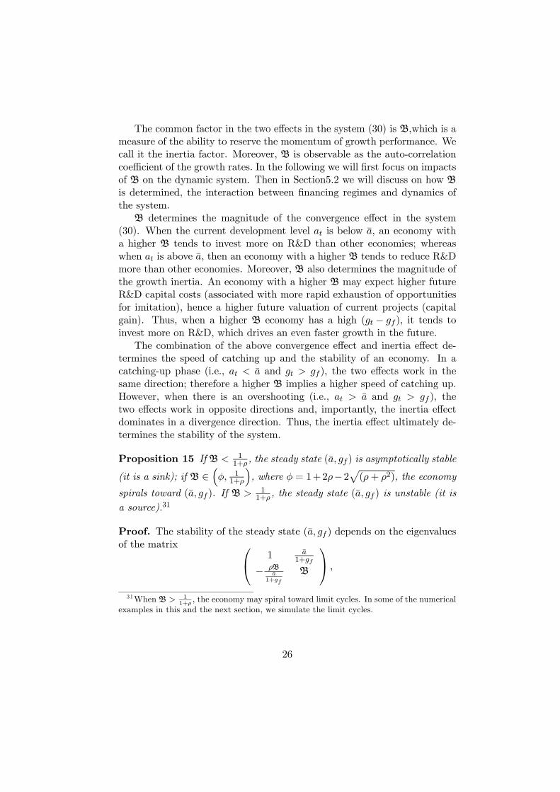
Proposition 15 IfB < 11+ρ , the steady state (a, gf ) is asymptotically stable

(it is a sink); if B ∈³φ, 1

1+ρ

´, where φ = 1+2ρ−2p(ρ+ ρ2), the economy

spirals toward (a, gf ). If B > 11+ρ , the steady state (a, gf ) is unstable (it is

a source).31

Proof. The stability of the steady state (a, gf ) depends on the eigenvaluesof the matrix 1 a

1+gf

− ρBa

1+gf

B

,

31When B > 11+ρ

, the economy may spiral toward limit cycles. In some of the numericalexamples in this and the next section, we simulate the limit cycles.

26

which are:

r1 =1

2(B+ 1) +

1

2

√η, r2 =

1

2(B+ 1)− 1

2

√η.

where η , B2−2B+1−4ρB. IfB < 11+ρ then |r1| < 1 and |r2| < 1, (a, gf )

is asymptotically stable; if B ∈³φ, 1

1+ρ

´, the two eigen values are complex

with the norm being smaller than unity, (a, gf ) is a cyclical attractor. IfB > 1

1+ρ , then |r1| > 1 and |r2| > 1, (a, gf ) is unstable.The essence of the above result is that when B is small, the inertia

effect is weak, and an economy will converge to its steady-state level with-out over-shooting; and when B is in the medium range, the inertia effectis strong enough to generate overshooting and contracting cycles, but notstrong enough to cause sustained cycles, which will occur when B is evenlarger. Next, we analyze how an economy’s B affects the economy’s conver-gence speed by solving the growth path. We start from the asymptoticallystable case, i.e., B ∈ (0, φ). In this case, the two real eigenvalues of thesystem are

r2 =1

2(B+ 1)− 1

2

√η < r1 =

1

2(B+ 1) +

1

2

√η < 1

and ∂r1∂B < 0. The associated eigenvectors are

v1 =

a( 12B− 12−12

√η)

ρB(1+gf)1

, v2 =

a( 12B− 12+ 12

√η)

ρB(1+gf)1

.

The solution confirms that when B is small, a higher B leads to a fasterconvergence toward the steady-state development level a.

Proposition 16 If B ∈ (0, φ) and a0 < a and g0 = gf , then when t issufficiently large, at increases with B, i.e., ∂at

∂B > 0, for at < a.

Proof. See Appendix B.Next, we analyze the cases where the value of B is at the medium level

and the growth path is cyclical, i.e., B ∈ ¡φ, φ

¢, where φ , 1 + 2ρ +

2p(ρ+ ρ2). Within this range ofB values, the two eigen values are complex

r1 =pB (1 + ρ)ei cosω, r2 =

pB (1 + ρ)e−i cosω

and their associated eigenvectors are

v1 =

Ãa√ρB

ρB(1+gf)e−iϕ

1

!, v2 =

Ãa√ρB

ρB(1+gf)eiϕ

1

!,

27

where ω , arccos

µ12+ 12B√

B(1+ρ)

¶is the angular velocity, ϕ , arccos

³ 12B− 1

2√ρB

´and the norm is |r1| =

pB (1 + ρ). Some properties of ω and ϕ are the

following:

ϕ ∈ (0, π) and ∂ϕ

∂B< 0; (32)

A useful approximate relation between ω and ϕ is given by

ω ≈Ãarccos

1p(1 + ρ)

!sinϕ, (33)

the derivation of which is provided in Appendix B. Solving the growth pathwe find that with a medium value ofB, although the growth path is cyclical,a higher B still leads to a faster catch up toward the steady-state positiona.

Proposition 17 If B ∈ ¡φ, φ¢ and a0 < a and g0 = gf , then the catching-up speed increases in B.

Proof. See Appendix B.The essence of Propositions 15 to 17 is that economies with a larger iner-

tia factorB have a stronger convergence effect and growth inertia; therefore,they tend to catch up faster. But they are also more likely to overshoot theirsteady-state targets. Relating these findings to the property of B, we havethe following empirically testable predictions.

Corollary 18 Ceteris paribus, economies with larger coefficients of auto-correlation in the growth rate tend to catch up faster, but they are morelikely to experience growth cycles.

The magnitude of the inertia factor B is determined by R&D selectionmechanisms used by financing regimes. In the next part we analyze thegrowth dynamics of economies under regimes m and s.

5.2 Catching up and Stability Properties of Financing Regimes

From eq. (31) a key factor which determines B is ∂C∗∂a

aC∗ , the steady-state

elasticity of R&D capital costs with respect to the development level. Itturns out the elasticity is affected by the R&D selection mechanism used bythe financing regime.

28

Lemma 19 Ceteris paribus, the R&D capital cost in both regimes, C∗ (λ (at))increases in at, i.e.,

∂C∗(λ(at))∂at

=K∗ζ (λ(at))

λ(at)λ0 (at) > 0, where ζ = s,m.

Proof. See Appendix B.Using Lemma 19 and eq. (31) we obtain inertia factor B under different

financing regimes

B =

Bs , δL−gfρ(1+gf)

λ0(a)aλ(a) K

∗s (λ (a)) under regime s,

Bm , δL−gfρ(1+gf)

λ0(a)aλ(a) K

∗m (λ (a)) under regime m.

(34)

To compare the dynamics of the two regimes, we study two economiesthat are identical in every aspect except for a difference in financing regimes.That is, we look at σ = σ∗ where the two regimes have identical steady statea∗; and they start from the same initial values (a0, g0) where a0 < a∗. Then,Proposition 20 implies that Bs > Bm.

Proposition 20 Bs > Bm at (a∗, σ∗).

Proof. By Proposition 12, if I3 > I3 then K∗s > K∗

m at (a∗, σ∗) ; conse-quently, Bs > Bm at (a∗, σ∗) .

Given growth inertia factors Bs and Bm are observable as growth rateauto-correlations, Proposition 20 not only makes testable predictions butalso, combined with some previous results, our model further predicts thatregime s (as compared to regime m) is more likely to fluctuate around itssteady state, which has a lower development level than regime m, althoughit may catch up faster.

Proposition 21 For an economy with σ = σ∗ and starting from the initialpoint (a0, g0) where a0 < a∗ and g0 = gf ,(1) the growth path under regime s is more likely to be cyclical than thatunder regime m.(2) it converges to its steady state faster under regime s than under regimem if Bs ≤ φ;(3) it reaches the level of a∗ earlier under regime s than under regime m ifBs ∈

¡φ, φ

¢.

Proof. See Appendix B.As has been shown, regime s gives greater advantages to more backward

economies, in particular economies with higher σ values. Nevertheless, somelow σ backward economies may benefit from adopting regime s at their early

29

stage of catching up as well. The following proposition characterizes anoptimal regime selection at different development stages. At an early stageof development, regime s is more efficient and catches up faster. However,as an economy approaches its steady-state development level, the financingregime should be changed to regime m.

Proposition 22 For an economy with σ ∈ (0, σ∗], there exists a thresholdvalue a such that if a0 < a, the optimal financing regime is regime s whenat < a and regime m when at ≥ a.

Proof. See Appendix B.Regime s is optimal at low development levels because it saves contract

enforcement costs and relies more on ex ante R&D selection, which is moreeffective at a low development level. When the development level is low,the growth path of an economy under regime s is independent from σ (seeeq. 24) such that an economy with σ < σ∗ can grow like an economy withσ ≥ σ∗. However, an economy with low σ can do better by switching toregime m when it is close to its steady-state development level.

Simulation results (Example 29) are shown in Appendix C to illustratethe above theoretical results.

6 Empirical and Policy Implications

A basic prediction of our theory on financing regimes (Proposition 20) isthat regime s has higher growth inertia B than regime m, where B is mea-sured as the growth rate auto-correlations. Although systematic tests ofthis prediction will be conducted during the next step of our research, somepreliminary observations seem to suggest that this prediction is consistentwith the data. Figure 4 in the following plots a lagged growth rate vs. thegrowth rate for the CEE economies (as proxies for regime s) and the WestEuropean (WE) economies (as proxies for regime m) for the period from1950 to 2000.32 The figure suggests that after controlling for the conver-gence effect, the average B of the CEE economies is higher than that of theWE economies: the slope for the CEE economies is positive, whereas theslope for the WE economies is negative.

32To be more precise, the horizontal axis of the figure is the lagged 5-year-average growthrate, and the vertical axis is the 5-year-average growth rate (net off the convergence effect,the adjustment of the U.S. 5-year-average growth rate, and the regression constant term).

30

g5_d_lag

g5_ee g5_pre_ee g5_we g5_pre_we

-.1 -.05 0 .05

-.05

0

.05

.1

Figure 4: Growth rate auto-correlations: CEE vs WE economies

Based on Proposition 20, our model (e.g., Proposition 21, etc.) predictsthat regime s is more likely to fluctuate around the steady-state develop-ment level, which is lower than that under regime m.33 To demonstratethe empirical implications of these predictions we provide the following sim-ulations.34 Using similar coordinates as those in Fig. 7 and 8 the verticalaxis is the difference between an economy’s growth rate and the world fron-tiers, gt − gf ; and the horizontal axis is the ratio between the economy’sdevelopment level and that of the world frontiers.

Fig. 5 is a simulation of regime m, which catches up first and thenconverges to its steady-state development level with moderate overshooting.Fig. 6 is a simulation of regime s for an economy with the same parametervalues as those for regime m. It demonstrates substantially larger growthcycles around a lower steady-state development level. Although we leaveformal tests of the predictions of our model for future work, the simulatedgrowth patterns of the two financing regimes seem consistent with the ob-served growth patterns of the two financing systems in Figures 7 and 8.

33Our model also predicts that the steady-state level of regime m is determined byinstitutional factor σ such that an economy with a higher σ should have a lower steady-state development level.34All the parameter values of the simulation are presented in Example 30 of Appendix

C.

31

-0.04

-0.02

0

0.02

0.04

0.06

0.08

0 10 20 30 40 50 60 70

at*100

gt-gf

Figure 5: A catch-up pattern of a regime m

-0.04

-0.02

0

0.02

0.04

0.06

0.08

0 5 10 15 20 25 30 35 40

at*100

gt-gf

Figure 6: A catch-up pattern of a regime s

With simultaneously endogenized financing and development, our modelhas rich policy implications. However, a complete exploration of the policyimplications of the model is beyond the scope of this paper. Here we brieflyillustrate some of the implications.

In reality, the choice (or change) of financing regime may be affectedby political institutions, legal restrictions, etc. For example, for a regimes, where the economy’s development level has caught up to a level that isclose to its steady state, it is optimal to switch to regime m at this time.However, this may not be implemented since some stakeholders who benefitfrom regime s may have strong incentives to block a regime change. As aresult, the economy may decline after an overshooting, which may triggeran economic/political crisis later. Therefore, a change of financial institutionmay occur as a consequence of a political regime change. Related to this,political regime changes (e.g., the collapse of centralized economies) or out-side pressures (e.g., reform conditions imposed by international institutionslike the IMF) may result in a different timing of regime change which can

32

be much worse than than optimal. Our model derives some useful policyimplications from the above-mentioned scenario.

Example 23 . Consider an economy starting from a0 < a∗ < a and g0 =gf . The following examples show the impacts of deviations from the second-best financing regime on the consequent development of the economy.

1. Optimal regime change: at first, regime s is chosen optimally, whichdelivers a high speed of catching up. Then the regime is changed at theoptimal timing to regime m, which guarantees a stable convergence tothe steady-state development level and growth rate (Panel a and b ofFig. 11 in Appendix C). After the regime change, the developmentlevel keeps increasing toward the steady-state level, while there is amoderate initial drop in the growth rate to adjust to the convergenceto the steady-state growth rate. Regarding in-house R&D as regime sand venture-capital-financed R&D as regime m, this may shed somelight on the impact of the rise of venture capital in the U.S. economysince the 1970s.

2. Late regime change: A reform takes place at the end of a positiveovershooting (Panel c and d of Fig. 11 in Appendix C). Immediatelyafter the regime change, there is a sharp drop in the growth rate whichmakes the development level decline as well. Then there is a recovery ofgrowth and the development level. Interpreting a centralized financialsystem as regime s, this may shed some light on the impact of failingto reform the financial system on time, as well as on the sharp declineof the transition economies after the change in financial systems.

3. Very late regime change: the regime change takes place at the end ofa negative overshooting (Panel e and f of Fig. 11 in Appendix C).Although the economy suffered low growth during the negative over-shooting, immediately after the regime change there was a second sharpdrop in the growth rate. This may reflect the experience of some of thetransition economies.

7 Conclusion

Our model suggests that under certain conditions related to legal institu-tions, some financial systems may be better than others in allowing an econ-omy to catch up faster. The same underlying force, however, may also result

33

in large growth cycles around lower steady-state development levels if finan-cial reform lags behind growth needs. Therefore, the timing of financialsystem reforms (e.g., financial liberalization) can play a critical role. More-over, our model implies that changes in the financial regime of an economyshould be conditional on the legal institutions in that economy. When legalinstitutions are very weak, the promotion of financial liberalization may im-pair the economy. This can shed some light on the problems of the formercentralized economies and their transition.

Our theory takes the decades-long debates on financial development andeconomic development,35 on alternative financial institutions one step fur-ther. It also provides alternative explanations for some important recentdiscoveries, such as the ‘irrelevance’ of financial structures (Beck and Levine,2002).

Furthermore, our theory has implications for the convergence/divergencedebate (e.g., Barro and Sala-I-Martin, 1995; Quah, 1996; Barro, 1997). Wepredict that when convergence will occur is conditional on the financialinstitutions and legal conditions.

Finally, our model focuses on one important aspect of the mechanisms offinancial institutions - R&D project financing/selection. We are fully awarethat financial institutions have other important features, such as affectingcapital investment in general, and affecting risk sharing between householdsand firms (Allen and Gale, 2000), etc. To make our point clear with a simplemodel, we abstract from many other mechanisms of financial institutions.These factors will be incorporated into our model in the future.

References

[1] Acemoglu, Daron, Aghion, Philippe and Zilibotti, Fabrizio (2003),“Distance to Frontier, Selection, and Economic Growth,” mimeo, MIT,Harvard, and UCL.

[2] Acemoglu, Daron, Simon Johnson, and James Robinson (2002), “Re-versal of Fortune: Geography and Institutions in the Making of the

35The debates on finance and development involve the following different majorviews/observations. Cameron et al. (1967), Rajan and Zingales (1998), and Carlin andMayer (2003) argue that some specific financial institutions are more helpful than oth-ers for economic development. Gerschenkron (1962) argues that the development stagemay determine the choice of financial institutions (backward countries might benefit frombanking institutions for catching up). In contrast, Robinson (1952) believes financial de-velopment follows economic growth. Lucas (1988) argues that financial development isnot important and it has been overemphasized.

34

Modern World Income Distribution,” Quarterly Journal of Economics,2002, 117: 1231-1294.

[3] Aghion, Philippe, and Howitt, Peter (1992), “A Model of GrowthThrough Creative Destruction,” Econometrica, 1992, 60, 323-51.

[4] Allen, Franklin, and Gale, Douglas (2000), Comparing Financial Sys-tems, Boston: MIT Press.

[5] Barro, Robert (1997), Determinants of Economic Growth: A Cross-Country Empirical Study, Cambridge and London: MIT Press.

[6] Barro, Robert, and Xavier Sala-I-Martin (1995), Economic Growth,New York: McGraw-Hill.

[7] Beck, Thorsten and Levine, Ross (2002), “Industry Growth and CapitalAllocation: Does Having a Market- or Bank-based System Matter?”,Journal of Financial Economics, 64, 147-180.

[8] Bergson, Abram (1989), Planning and Performance in SocialistEconomies: The USSR and Eastern Europe, London: Unwin Hyman.

[9] Bolton, Patrick and David S. Scharfstein (1996), “Optimal Debt Struc-ture and the Number of Creditors,” Journal of Political Economy, 104,1-25.

[10] Cameron, Rondo et al. (1967), Banking in the Early Stages of Indus-trialization: A Study in Comparative Economic History, New York:Oxford University Press.

[11] Carlin, Wendy, and Colin Mayer (2003), “Finance, Investment andGrowth,” mimeo, UCL and Oxford.

[12] Demetriades, Panicos and Siong Hook Law (2004), “Finance, Institu-tions and Economic Growth,” mimeo, Leicester University.

[13] Dewatripont, Mathias, and Maskin, Eric (1995), “Credit and Effi-ciency in Centralized and Decentralized Economies.” Review of Eco-nomic Studies, 62, 541-555.

[14] Engerman, Stanley and Sokoloff, Kenneth (2000) “Institutions, FactorEndowments, and Paths of Development in the New World,” Journalof Economic Perspectives, 3, 217-232.

35

[15] Gerschenkron, Alexander (1962), Economic Backwardness in HistoricalPerspective, Cambridge MA: Harvard University Press.

[16] Glaeser, Edward, Simon Johnson, and Andrei Shleifer (2001), “Coasevs. Coasians,” Quarterly Journal of Econmics, 116, 853-899.

[17] Gompers, Paul and Lerner, Josh (2001), The Money of Invention: HowVenture Capital Creates New Wealth. Boston: Harvard Business Press.

[18] Grossman, Gene, and Elhaman Helpman (1991), “Quality Ladders inthe Theory of Growth,” Review of Economic Studies, 58, 43-61.

[19] Hanson, P., and K. Pavitt (1987), The Comparative Economics ofResearch Development and Innovation in East and West: A Survey,Switzerland: Hardwood Academic Publishers.

[20] Hart, Oliver and Moore, John (1995), “Debt and Seniority: an Analysisof the Role of Hard Claims in Constraining Management,” AmericanEconomic Review, June, 85, 567-586.

[21] Hirsch, Morris W. and Stephen Smale (1974), Differential Equations,Dynamical Systems, and Linear Algebra, San Diego: Academic Press.

[22] Huang, Haizhou and Xu, Chenggang (2003), “Financial Syndicationand R&D,” Economics Letters.

[23] Huang, Haizhou and Xu, Chenggang (1999), “Institutions, Innovations,and Growth,” American Economic Review, 89: 438-443, May 1999.

[24] Huang, Haizhou and Xu, Chenggang (1998), “Financial Budget Con-straints and the Optimal Choices of R&D Project Financing,” Journalof Comparative Economics, 26, 62-79.

[25] King, Robert, and Levine, Ross (1993), “Finance and Growth: Schum-peter Might Be Right,” Quarterly Journal of Economics, 108, 717-737.

[26] Kornai, Janos (1992), The Socialist System: The Political Economy ofCommunism, New York and London: Princeton University Press andOxford University Press.

[27] Kornai, Janos (1979), “Resource-Constrained versus Demand-Constrained Systems,” Econometrica, 47, 801-819.

[28] Kornai, Janos, Maskin, Eric, and Roland, Gerard (2003), “Understand-ing the Soft Budget Constraint,” Journal of Economic Literature, 2003.

36

[29] Lamoreaux, Naomi (1986), “Banks, Kinship, and Economic Develop-ment: the New England Case,” Journal of Economic History, 46, 647-667.

[30] La Porta, Rafael, Lopez-de-Silanes, Florencio, Shleifer, Andrei andVishny, Robert W. (1998), ‘Law and Finance,’ Journal of PoliticalEconomy, 106, 1113-1155.

[31] Linz, S., and J. Thorton (1988), ”A Preliminary Analysis of the Demandfor Innovation: Evidence from the Soviet Interview Project,” WorkingPaper #56, University of Washington.

[32] Lucas, Robert (1988), “On the Mechanics of Economic Development,”Journal of Monetary Economics, 22, 3-42.

[33] Maddison, Angus (2003), The World Economy — Historical Statistics,Paris: OECD Publications Service.

[34] Maskin, Eric, and Xu, Chenggang (2001), “Soft Budget Constraint The-ories: From Centralization to the Market,” Economics of Transition,2001.

[35] Matsuyama, Kiminori (2001), ‘Growing through cycles in an infinitelylived agent economy,’ Journal of Economic Theory, 100, 220-234.

[36] Matsuyama, Kiminori (1999), ‘Growing through cycles,’ Econometrica,67, 335-347.

[37] Milgrom, P. (1988), ”Employment Contracts, Influence Activities andOrganization Design,” Journal of Political Economy, 96, 42-60.

[38] National Science Board (1989), Science & Engineering Indicators —1989, Washington, D.C.: US Government Printing Office.

[39] Poznanski, K. (1985), ”The Environment for Technological Changein Centrally Planned Economies,” Working Paper no.718, The WorldBank.

[40] Qian, Yingyi, and Xu, Chenggang (1998), “Innovation and Bureau-cracy Under Soft and Hard Budget Constraints,” Review of EconomicStudies, 65, 151-164.

[41] Quah, Danny (1996), “Twin Peaks: Growth and Convergence in Modelsof Distribution Dynamics,” Economic Journal, 106, 1045-1055.

37

[42] Rajan, Raghuram, and Zingales, Luigi (1998), “Financial Dependenceand Growth,” American Economic Review, 88, 559-586.

[43] Rajan, Raghuram G. and Zingales, Luigi (2001), “Financial Systems,Industrial Structure, and Growth,” Oxford Review of Economic Policy,17, 467-482.

[44] Rajan, Raghuram G. and Zingales, Luigi (2003), Saving Capitalismfrom the Capitalists: Unleashing the Power of Financial Markets toCreate Wealth and Spread Opportunity, New York: Crown Business.

[45] Robinson, J. (1952), The Rate of Interest and Other Essays, London:Macmillan, 67-142.

[46] Romer, Paul (1990), “Endogenous Technological Change.” Journal ofPolitical Economy, 98, 71-102.

[47] Schumpeter, Joseph (1936), The Theory of Economic Development,Cambridge, MA: Harvard University. Press.

[48] Xu, Chenggang and Katharina Pistor (2002), “Law Enforcement underIncomplete Law: Theory and Evidence from Financial Market Regula-tion,” LSE STICERD Theory Discussion Paper No. TE/02/442.

38

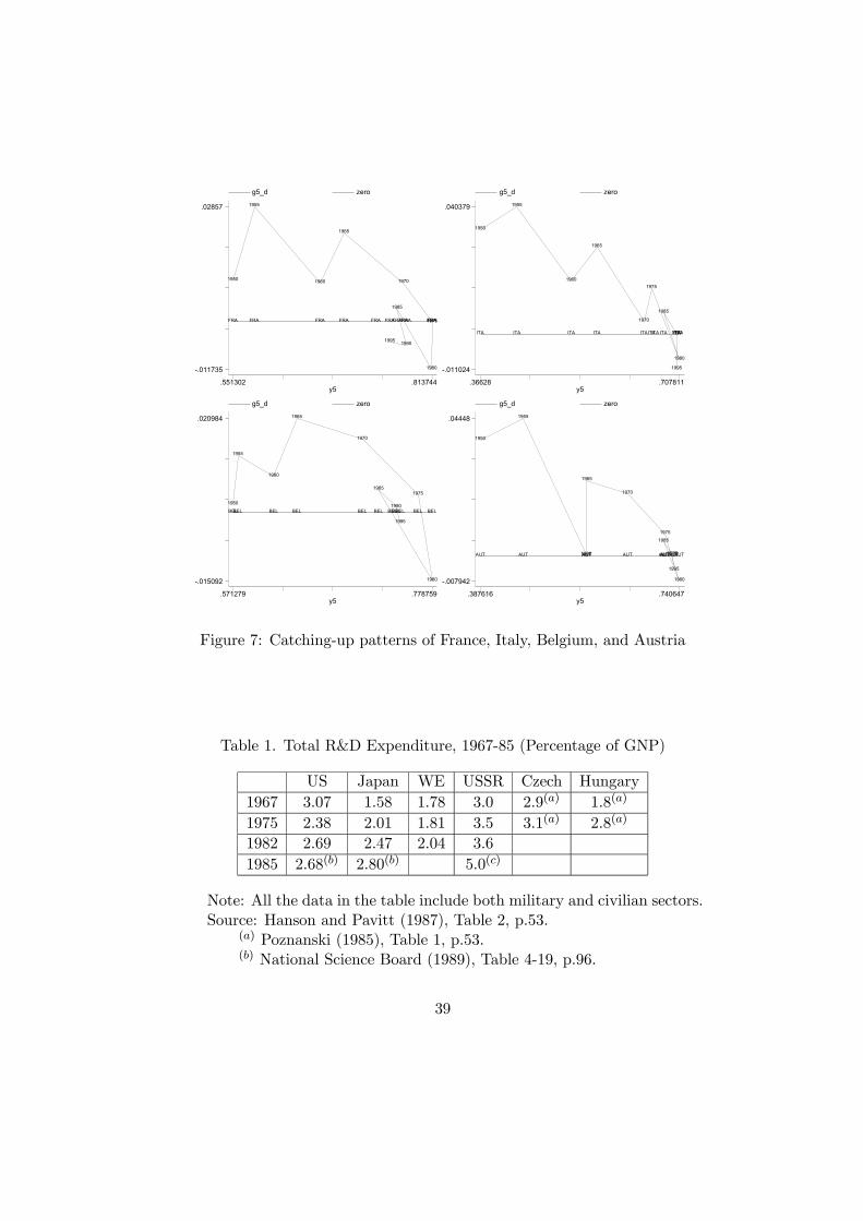
y5

g5_d zero

.551302 .813744

-.011735

.02857

1950

1955

1960

1965

1970

1975

1980

1985

19901995

FRA FRA FRA FRA FRA FRAFRAFRAFRAFRAFRA

y5

g5_d zero

.36628 .707811

-.011024

.040379

1950

1955

1960

1965

1970

1975

1980

1985

1990

1995

ITA ITA ITA ITA ITAITA ITAITA ITAITAITA

y5

g5_d zero

.571279 .778759

-.015092

.020984

1950

1955

1960

1965

1970

1975

1980

1985

1990

1995

BELBEL BEL BEL BEL BEL BELBEL BELBELBEL

y5

g5_d zero

.387616 .740647

-.007942

.04448

1950

1955

1960

1965

1970

1975

1980

1985

1990

1995

AUT AUT AUTAUT AUT AUT AUTAUTAUTAUTAUT

Figure 7: Catching-up patterns of France, Italy, Belgium, and Austria

Table 1. Total R&D Expenditure, 1967-85 (Percentage of GNP)

US Japan WE USSR Czech Hungary1967 3.07 1.58 1.78 3.0 2.9(a) 1.8(a)

1975 2.38 2.01 1.81 3.5 3.1(a) 2.8(a)

1982 2.69 2.47 2.04 3.61985 2.68(b) 2.80(b) 5.0(c)

Note: All the data in the table include both military and civilian sectors.Source: Hanson and Pavitt (1987), Table 2, p.53.

(a) Poznanski (1985), Table 1, p.53.(b) National Science Board (1989), Table 4-19, p.96.

39

y5

g5_d zero

.235746 .356485

-.033063

.027371

1950

1955

19601965

1970

1975

1980

1985

1990

1995

HUN HUN HUNHUNHUN HUNHUNHUNHUNHUN HUN

y5

g5_d zero

.220378 .356669

-.043029

.039601

1950

1955

1960

1965

1970

1975

1980

1985

1990

1995

POLPOL POLPOL POL POLPOLPOLPOL POL POL

y5

g5_d zero

.106723 .230963

-.056214

.0406621950

1955

1960

1965

1970

1975

1980

1985

1990

1995

ROM ROM ROM ROM ROM ROMROMROMROMROMROM

y5

g5_d zero

.15468 .37675

-.11464

.027748

1950

1955

1960

1965

1970

19751980

1985

1990

1995

USSRUSSR USSRUSSR USSRUSSRUSSRUSSRUSSRUSSRUSSR

Figure 8: Catching-up pattern of the USSR, Hungary, Poland, and Romania

40

(c) Linz and Thorton (1988).Table 2. Civilian Sector R&D Expenditure Comparison (percentage of

GNP)

US Japan France West Germany UK USSR1967 1.2 1.8 1.5 1.6 1.9 1.4

Note: Defense and space sector R&D expenditures excluded for all coun-tries.

Source: Bergson (1989), Table 11, p.125.

Table 3. Scientists and Engineers in R&D, USSR vs. U.S.

USSRmillion

U.S.million

USSRper 10,000 workers

U.S.per 10,000 workers

1950 1.25 1.59 14.7 26.21960 2.73 3.81 27.5 55.81970 6.62 5.47 54.2 66.81975 8.74 5.35 66.0 61.5

Note: Scientists and engineers in both countries exclude humanities spe-cialists, social scientists, and psychologists.

Source: Bergson (1989), Table 12, p.126.

41

A Appendix A

AssumptionsA-1: I2+ I3

1+ρ+w1+ρ >

δαLwρ (the cost of a bad project at stage 2 is higher

than the upper bound of profit).A-2: I1 + I2 +

w1+ρ ≥ I3

1+ρ (the cost of a bad project at stage 3 is lowerthan the cost of a good project).

A-3: I3+F1+ρ > δαLw

ρ (the cost of a bad project at stage 3, conditional onregime m, is more expensive than the upper bound of profit).

To prove Lemma 1, let us first prove the following Lemma.

Lemma 24 From assumptions A-1, A-2, and A-3, it follows that in anyequilibrium with a positive growth rate,(1) I2 + I3

1+ρ +w1+ρ > δ

P∞τ=t+1 (1 + ρ)−(τ−t) πτ > I3

1+ρ

(2) I1 + I2 +w1+ρ < δ

P∞τ=t+1 (1 + ρ)−(τ−t) πτ .

(3) δP∞

τ=t+1 (1 + ρ)−(τ−t) πτ < I3+F1+ρ

Proof. Since πτ = αL1tw1+ρ and L1t ≤ L, δ

P∞τ=t+1 (1 + ρ)−(τ−t) πτ ≤ δαLw

ρ

holds, i.e., δαLwρ is an upper bound to the expected profit of a project in

any equilibrium with a positive growth rate. Consequently, from A-1 andA-2, it follows that I2 + I3

1+ρ +w1+ρ > δαLw

ρ ≥ δP∞

τ=t+1 (1 + ρ)−(τ−t) πτ >

I1+ I2+w1+ρ ≥ I3

1+ρ , which implies (1). On the other hand, since the cost ofa good project, i.e., I1+ I2+

w1+ρ , is a lower bound to the expected profit of

a project in any equilibrium with a positive growth rate, i.e., I1+I2+w1+ρ <

δP∞

τ=t+1 (1 + ρ)−(τ−t) πτ , then (2) holds. Finally by A-3, I3+F1+ρ > δαLw

ρ ≥δP∞

τ=t+1 (1 + ρ)−(τ−t) πτ holds, which implies (3).Sketch of proof of Lemma 1: Applying the above result (3), if ex

ante some financiers decide to finance a project jointly, an entrepreneur, whodiscovers that the project is bad at stage 1 will stop it right away to avoid acostly liquidation at stage 2, since for the entrepreneur the private benefitsare b1 > b2. As a result, under multi-financier financing, all bad projectswill be terminated at date 1.

However, if a project is financed by one financier, when the financier dis-covers that the project is a bad one at stage 2, given that earlier investmentsare sunk, according to the above result (2), continuing the bad project isex post profitable, the financier will choose to refinance the project. Antici-pating this, at stage 1 when an entrepreneur with a bad project realizes thetype of the project, the entrepreneur will not report the private information

42

about the type of the project. Thus, the financier will always refinance abad project.36

B Appendix B

Proof of Lemma 4First consider regime s. Since Cs is not a function of σ, it follows that

∂θ∗s∂σ = 0,

∂C∗s∂σ = 0 and ∂K∗s

dσ = 0.Under regime m, there is an interior optimal precision θ∗m for λ >

0 (Lemma 25). At the point θm = θ∗m, the derivative∂C∗m∂σ = ∂Cm

∂σ =qθ+qθqθm

F > 0. Differentiating the equation ∂C∗m∂θm

= 0 w.r.t. σ and reor-

ganizing, it follows that ∂θ∗mdσ = qF

λψ00(θ∗m)θ∗m> 0 and ∂K∗m

∂σ = ∂K∗m∂θ

∂θ∗m∂σ =

λψ0(θ∗m)θ∗m−λψ(θ∗m)qθ∗2m

qFλψ00(θ∗m)θ∗m

> 0.Now consider the special case: σ = 0. In the following we are going to

show the R&D capital cost is lower under regime m, i.e., C∗m < C∗s , whereC∗s = K∗

s +qθ∗s

qθ∗s+qθ∗s

I31+ρ+I1+I2+

w1+ρ and C

∗m = K∗

m+qθ∗m+qθ

∗m

qθ∗mI1+I2+

w1+ρ .

The comparison is not straightforward, and the plan for doing it is tofind a suboptimal level of prescreening, Km, under regime m such thatthe corresponding R&D capital cost Cm is strictly lower than C∗s , i.e.,C∗m ≤ Cm < C∗s .Let Km be chosen such that Km = K∗

s , i.e.,λψ(θm)qθm

= λψ(θ∗s)qθ∗s+qθ

∗s. Then

Cm− C∗s =qθmqθm

I1− qθ∗s

qθ∗s+qθ∗s

I31+ρ =

qθmqθm

³I1 − qθ

∗s

qθ∗s+qθ∗s

θmθm

I31+ρ

´. It follows from

reorganizing λψ(θm)qθm

= λψ(θ∗s)qθ∗s+qθ

∗sthat ψ (θm)

¡qθ∗s + qθ

∗s

¢= ψ (θ∗s) qθm. It is

useful to solve for θm (approximately) by linearizing the left-hand side of theequation around θ∗s:

¡ψ (θ∗s) + ψ0 (θ∗s) (θm − θ∗s)

¢ ¡qθ∗s + qθ

∗s

¢ ≈ ψ (θ∗s) qθm,

which gives rise to θm ≈ (ψ0(θ∗s)θ∗s−ψ(θ∗s))(qθ∗s+qθ∗s)ψ0(θ∗s)(qθ∗s+qθ

∗s)−ψ(θ∗s)q

. With this result, we can

approximate the term qθ∗s

qθ∗s+qθ∗s

θmθmand derive that following:

qθ∗s

qθ∗s+qθ∗s

θmθm≈ q ψ0(θ∗s)θ∗s−ψ(θ∗s)

ψ0(θ∗s)θ∗s−ψ(θ∗s)+(ψ0(θ∗s)(1−2θ∗s)+2ψ(θ∗s))q .

The term ψ0(θ∗s)θ∗s−ψ(θ∗s)ψ0(θ∗s)θ∗s−ψ(θ∗s)+(ψ0(θ∗s)(1−2θ∗s)+2ψ(θ∗s))q turns out to be bounded by

1 from below, which is equivalent to ψ (θ∗s) − ψ0 (θ∗s)¡θ∗s − 1

2

¢ ≤ 0. To seethis, note that by the mean value theorem, ψ (θ∗s)−ψ

¡12

¢= ψ0

³θ´ ¡

θ∗s − 12

¢36The first and second parts of this lemma are variations of Dewatripont and Maskin

(1995) and Huang and Xu (2003) respectively, with working assumptions of reduced formtransaction cost and A-3.

43

where θ ∈ £12 , θ

∗s

¤. It follows that ψ0

³θ´≤ ψ0 (θ∗s) due to the assump-

tion that ψ00 (·) > 0 (by A-5). Then ψ (θ∗s) − ψ¡12

¢= ψ0

³θ´ ¡

θ∗s − 12

¢ ≤ψ0 (θ∗s)

¡θ∗s − 1

2

¢, which implies that ψ (θ∗s)−ψ0 (θ∗s)

¡θ∗s − 1

2

¢ ≤ 0. The usefulimplication of this result is that (conditional on the approximation error

being sufficiently small) qθ∗s

qθ∗s+qθ∗s

θmθm

> q, hence,

C∗m − C∗s ≤ Cm − C∗s ≤ qθmqθm

³I1 − q I3

1+ρ

´< 0 since q I3

1+ρ > I1 (by A-4).Proof of Proposition 5Denote by σ (λ) the solution to C∗s = C∗m for a given λ > 0. Lemma

4 suggests that C∗s > C∗m as σ = 0 and ∂C∗m∂σ > 0. It is also easy to verify

that C∗m → ∞ as σ → ∞. Then it follows that σ (λ) exists (by the mean-value theorem) and is unique. Consequently, according to Proposition 3 andLemma 4, C∗s < C∗m and ζ∗ = s if and only if σ > σ (λ).

Proof of Proposition 8Suppose at equilibrium the steady-state level of relative development is

a = a, but there exists a > a which can be achieved by an alternativefinancing regime, denoted by ζ, in the steady state. Hence, C∗ζ (a;σ) =C∗ (a;σ) = C∗f (by Lemma 7) and C∗ζ (a;σ) < C∗ (a;σ) (by Proposition 19).Combining the two conditions gives rise to C∗ζ (a;σ) < C∗ζ (a;σ) and applyingProposition 19 again, we have a < a, which contradicts the assumption thata > a.

Proof of Lemma 12For each value of I3 equationK∗

s = K∗m define a curve σk (a; I3) which di-

vides the (a, σ) space, (see Figure 9) and σk (a; I3) increases in I3 (see Lemma27). Define I3 , inf I3 : σk (a; I3) ≥ σss (a) for all a ∈ (0, 1). Since σk (a; I3)increases in I3, σk (a; I3)→∞ as I3 →∞ and σss (a) is finite, it follows thatI3 is finite. So σk (a; I3) > σss (a) as I3 > I3 (by definition), which impliesthat K∗

s > K∗m along the σss (a) curve for a > 0.

Proof of Proposition 13In the steady state, regime m is associated with σ ≤ σ∗ and a ≥ a∗,

regime s is associated with a = a∗; if I3 > I3 then K∗m < K∗

s (by Proposition

12). Consequently, θ∗m < θ∗s and qθ∗m < qθ∗s+qθ

∗s. Finally, the fact

∂(qθ+qθ)∂θ <

0 as q < 12 implies that qθ

∗m + qθ

∗m > qθ∗s + qθ

∗s as q <

12 .

Proof of Proposition 14

The algebraic fact ∂∂θ

qθqθ+qθ

=−q(qθ+qθ)−qθ(q−q)

(qθ+qθ)2 = −qq

(qθ+qθ)2 < 0 is to be

used, together with Lemma 25 and A-5, to derive the following:∂∂a

qθ∗m

qθ∗m+qθ∗m=³

∂∂λ

qθ∗m

qθ∗m+qθ∗m

´λ0 (a) =

³∂

∂θ∗mqθ∗m

qθ∗m+qθ∗m

´∂θ∗m∂λ λ0 (a) > 0.

44

σss

0

σk )( 3I(

σk(I3)

Ks> Km

Ks< Km

a

σ

Figure 9: σk > σss as I3 > I3

Proof of Proposition 16We first solve the growth path through the following steps.

Step 1: The general (non-periodical) solution of the linear equation system

isµ

atgt

¶=

µagf

¶+¡v1 v2

¢µ rt1 00 rt2

¶µC1C2

¶.

Step 2: Consider an initial valueµ

a0g0

¶such that a0 < a and g0 = gf ,

which determines thatµ

C1C2

¶=¡v1 v2

¢−1µ a0 − a0

¶. It is easy to

verify that¡v1 v2

¢−1= −ρB(1+gf)

a√η

1 − a( 12 (B−1)+ 12

√η)

ρB(1+gf)

−1 a( 12 (B−1)−12

√η)

ρB(1+gf)

, and it follows that

µC1C2

¶= −ρB(1+gf)

a√η

µ(a0 − a)− (a0 − a)

¶.

Step 3: The special solution then isµatgt

¶=

µagf

¶− ρB(1+gf)(a0−a)

a√η

¡rt1v1 − rt2v2

¢=

µagf

¶− ρB(1+gf)(a0−a)

a√η rt1

µv1 −

³r2r1

´tv2

¶.

Since³r2r1

´t ≈ 0 as t is sufficiently large, thenµat − agt − gf

¶≈ −ρB(1+gf)(a0−a)

a√η rt1v1 .That is,

µat − agt − gf

¶converges to

45

µ00

¶along the straight line projected by the eigenvector v1.

In particular, at = a− 12 (a− a0) r

t1

µ³1−B√

η + 1´−³r2r1

´t ³1−B√

η − 1´¶

< a

Approximately, at ≈ a− 12 (a− a0) r

t1

³1−B√

η + 1´

since³r2r1

´t ≈ 0 as t is sufficiently large.∂at∂B ≈ −12 (a− a0) r

t−11

Ãt³1−B√

η + 1´

∂r1∂B(−)

+ r1∂∂B

³1−B√

η

´!> 0

as t is sufficiently large.Derivation of the approximate relation between ω and ϕ

Recall the definitions of ω and ϕ : ω , arccos

µ12+12B√

B(1+ρ)

¶and ϕ ,

arccos³ 12B− 1

2√ρB

´Solve

√B as a function of ϕ as follows,

√B =

√ρ (cosϕ)+

p(ρ (cosϕ) + 1)therefore,

ω = arccos1+ρ cos2 ϕ+

√ρ(cosϕ)

√(ρ cos2 ϕ+1)³√

ρ cosϕ+√(ρ cos2 ϕ+1)

´√(1+ρ)

Denote cosϕ by Φ so that : ω = arccos1+ρΦ2+

√ρΦ√(ρΦ2+1)³√

ρΦ+√(ρΦ2+1)

´√(1+ρ)

=

arccos1+ρΦ2+

√ρΦ√(ρΦ2+1)µ√

ρΦ+√(ρΦ2+1)

¶√(1+ρ)

√1−Φ2 sinϕ

Linearizing

arccos1+ρΦ2+

√ρΦ√(ρΦ2+1)µ√

ρΦ+√(ρΦ2+1)

¶√(1+ρ)

√1−Φ2 around Φ = 0

arccos1+ρΦ2+

√ρΦ√(ρΦ2+1)µ√

ρΦ+√(ρΦ2+1)

¶√(1+ρ)

√1−Φ2 ≈ arccos 1√

(1+ρ)+ 0Φ

ω ≈µarccos 1√

(1+ρ)

¶sinϕ

Proof of Proposition 17Step 1: The general (periodical) solution of the linear equation system

isµatgt

¶=

µagf

¶+³p

B (1 + ρ)´tà a

√ρB

ρB(1+gf)e−iϕ a

√ρB

ρB(1+gf)eiϕ

1 1

!µeitω 00 e−itω

¶µC1C2

¶.

Step 2: Consider an initial valueµ

a0g0

¶such that a0 < a and g0 = gf , then

we have

46

µC1C2

¶=

Ãa√ρB

ρB(1+gf)e−iϕ a

√ρB

ρB(1+gf)eiϕ

1 1

!−1µa0 − a0

¶=

ρB(1+gf)(a0−a)2a√ρB sinϕ

µi−i

¶.

Step 3: the special solution isµatgt

¶=

a+³p

B (1 + ρ)´t

(a−a0)sinϕ sin (tω − ϕ)

gf +³p

B (1 + ρ)´t

(a−a0)sinϕ

√ρB(1+gf)

a sin (tω)

. The trajec-

tory is a clockwise spiral around the steady state. The time for the trajec-tory to pass at = a from the left for the first time is the solution to theequation:tω − ϕ = 0 ⇒ t = τ , ϕ

ω , the smaller τ , the faster the speed of catchingup. The following proposition reports the result for medium-range valuesof B that an economy with a larger B has a faster catching up. Using the

approximation: ω ≈µarccos 1√

(1+ρ)

¶sinϕ, it follows that ∂τ

∂B = ∂∂B

ϕω ≈

∂∂B

ϕµarccos 1√

(1+ρ)

¶sinϕ

= 1µarccos 1√

(1+ρ)

¶³ ∂∂B

ϕsinϕ

´(+)

∂ϕ∂B(−)

< 0 as B ∈ ¡φ, φ¢ .Proof of Proposition 19

In Lemma 25 we establish that∂C∗ζ∂λ > 0 for ζ = s,m. Noticing that

K∗s , λψ(θ∗s)

qθ∗s+qθ∗s, K∗

m , λψ(θ∗m)qθ∗m

, λ = λ (at) and C∗ = min¡C∗s , C∗m

¢, it follows

that under regime s, ∂C∗(λ(at))∂at

= ∂C∗s∂λ λ0 (at) =

K∗sλ(at)

λ0 (at) > 0; under regime

m, ∂C∗(λ(at))∂at

= dC∗mdλ λ0 (at) =

K∗mλ(at)

λ0 (at) > 0.Proof of Proposition 21When I3 > I3, for an economy with σ = σ∗, Bs > Bm in the steady

state (Lemma 12).If Bs ≤ φ then Bm < φ. By Proposition 16 ∂at

∂B > 0 as B < φ for sufficientlylarge t, which implies that at,s > at,m, i.e., the speed to converge to thesteady state is faster under regime s, where at,s and at,h are the values of atunder regime s and regime m.If Bs ∈

¡φ, φ

¢then Bm < φ. By Proposition 17 ∂τ

∂B < 0 as B ∈ ¡φ, φ¢;therefore τ s < τm if τm is finite, where τ s and τm are the values of τ underregime s and regime m respectively. As a result, at,s reaches a∗ earlier thanat,m.It is possible that Bs > φ > Bm but not the reverse. Consequently, byProposition 15 the growth rate is more likely to be cyclical under regime sthan under regime m.

Proof of Proposition 22

47

Define a such that σc (a) = σ ≤ σ∗ and a ≤ a∗. By Proposition 5 regimes is chosen when a0 ≤ at < a and regime m is chosen when a ≤ at < awhere a ≥ a∗ by Proposition 11.

Lemma 25 For λ > 0 there is a unique interior solution, θ∗ζ ∈ (1/2, 1),to the minimization problem: minθζ Cζ for ζ = s,m, with the following

comparative statics:∂θ∗ζ∂λ < 0,

∂C∗ζ∂λ > 0 and

∂2C∗ζ∂λ2

< 0.

Proof. First consider the case: ζ = m. Cm =λψ(θm)qθm

+ qθm+qθmqθm

(σF + I1)+

I2 +w1+ρ is twice continuously differentiable in θm. At the point θm = 1/2,

Cm is finite; the derivative ∂Cm∂θm

= 2λψ0( 12)

q − 4 qq (I1 + σF ) is negative since

λ ≤ 2qI1ψ0( 12)

(by assumption A-5). If the solution to ∂Cm∂θm

= 0 does not exist, it

must be the case that ∂Cm∂θm

< 0 for all θm ≤ [1/2, 1] and hence, Cm is smallerat θm = 1 than θm = 1/2; but this contradicts the fact that Cm is positiveinfinity at θm = 1. So we conclude that an interior solution to ∂Cm

∂θm= 0 must

exist; let it be denoted by θ∗m. At the point θm = θ∗m, using the equationimplied by ∂Cm

∂θm= 0, we can write down the second order derivative in the

simple form: ∂2C∗m∂θ2m

= λψ00(θ∗m)θ∗2mqθ∗3m

, which is positive. Thereby, we infer that

the interior critical point (solution to ∂Cm∂θm

= 0) is unique (otherwise, at leastone of the solutions is not a local minimum, which contradicts the fact that∂2Cm∂θ2m

> 0 at each of the solutions) and is the global minimum.

Now we focus attention to the point θ = θ∗m. Differentiating the equation∂C∗m∂θ = 0 w.r.t. λ and reorganizing, it follows that ∂θ∗m

∂λ = ψ(θ∗m)−ψ0(θ∗m)θ∗mλψ00(θ∗m)θ∗m

<

0. Now it is straightforward to derive the following comparative statics:∂C∗m∂λ = ∂Cm

∂λ + ∂Cm∂θm

dθ∗mdλ = ∂Cm

∂λ = ψ(θ∗m)qθ∗m

> 0 and ∂2C∗m∂λ2

= ∂∂λ

³ψ(θ∗m)qθ∗m

´=

ddθ∗m

³ψ(θ∗m)qθ∗m

´∂θ∗m∂λ < 0.

The same argument goes through for the case: ζ = s. Some particular pointswe need to make are that λ < 2qqI3

ψ0( 12)(1+ρ)is satisfied as (1 + ρ) I3 >

I1q (by

A-4)) and λ ≤ 2qI1ψ0( 12)

(by A-5); that ∂C∗s∂λ = ∂Cs

∂λ = ψ(θ∗s)qθ∗s+qθ

∗s.

Lemma 26 ∂θ∗s∂I1

= 0, ∂θ∗s∂I3

> 0, ∂K∗s∂I1

= 0, ∂K∗s∂I3

> 0 and ∂C∗s∂I3

> 0 as λ > 0;∂θ∗m∂I1

> 0, ∂θ∗m∂I3

= 0, ∂K∗m∂I1

> 0, ∂K∗m∂I3

= 0 as λ > 0.

Proof. For the case of regime s, the starting point for deriving the set of

comparative statics is the FOC: ∂Cs∂θ = 0, or more precisely,λψ0(θ∗s)(qθ∗s+qθ

∗s)−λψ(θ∗s)(q−q)qq =

48

I31+ρ . Differentiating the both sides of the equation w.r.t. I1 and I3 respec-tively and reorganizing, it follows thatλψ00(θ∗s)(qθ∗s+qθ

∗s)

qq∂θ∗s∂I1

= 0⇒ ∂θ∗s∂I1

= 0;λψ00(θ∗s)(qθ∗s+qθ

∗s)

qq∂θ∗s∂I3

= 11+ρ ⇒ ∂θ∗s

∂I3= qq

(1+ρ)λψ00(θ∗s)(qθ∗s+qθ∗s)

> 0.

Also ∂K∗s∂I1

= ∂∂I1

λψ(θ∗s)qθ∗s+qθ

∗s= ∂

∂θ∗sλψ(θ∗s)qθ∗s+qθ

∗s

∂θ∗s∂I1

= 0,∂K∗s∂I3

= ∂∂I3

λψ(θ∗s)qθ∗s+qθ

∗s= ∂

∂θ∗sλψ(θ∗s)qθ∗s+qθ

∗s

∂θ∗s∂I3

> 0 and dC∗sdI3

= ∂C∗s∂I3

= qθ∗s

qθ∗s+qθ∗s

11+ρ > 0

For the case of regimem, the FOC, ∂C∗m

∂θ = 0 implies that λψ0(θ∗m)θ∗m−λψ(θ∗m)q =

I1 + σF .Differentiating the both sides of the equation w.r.t. I1 and I3 respectivelyand reorganizing, it follows thatλψ00(θ∗m)θ∗m

q∂θ∗m∂I1

= 1⇒ ∂θ∗m∂I1

= qλψ00(θ∗m)θ∗m

> 0 andλψ00(θ∗m)θ∗m

q∂∗m∂I3

= 0⇒ ∂θ∗m∂I3

= 0. Consequently,∂K∗m∂I1

= ∂∂I1

λψ(θ∗m)qθ∗m

= ∂∂θ∗m

λψ(θ∗m)qθ∗m

∂θ∗m∂I1

> 0

and ∂K∗m∂I3

= ∂∂I3

λψ(θ∗m)qθ∗m

= ∂∂θ∗m

λψ(θ∗m)qθ∗m

∂θ∗m∂I3

= 0.

Lemma 27 ∂σk∂I3

> 0 and ∂σss∂I3

= 0.

Proof. Differentiating the equation K∗m = K∗

s w.r.t. to σ and I3 and

reorganizing, it results in ∂σk∂I3

=∂K∗s∂I3∂K∗m∂σ

> 0 since ∂K∗m∂σ > 0 and ∂K∗s

∂I3> 0 (by

Lemma 4 and 26). Also, since I3 does affect regime m at all, it is obviousthat ∂σss

∂I3= 0.

Lemma 28 The steady state (0, g) where g , ρ(1+ρ)αw

¡C∗ (λ (a))− C∗ (λ (0))

¢+

gf , is unstable.

Proof. Linearizing the growth equation (24) around (0, g) results inµat+1

gt+1 − g

¶≈µ

B1 0−B2 0

¶Ãat

gt −³ρ(1+ρ)αw

¡C∗ (λ (a))− C∗ (λ (0))

¢+ gf

´ !,where B1 = 1 +

ρ(1+ρ)αw (C∗(λ(a))−C∗(λ(0)))

1+gfand B2 =

ρ(1+ρ)αw

∂C∗(λ(0))∂λ

¡λ0 (0)

¢.

The transition matrixµ

B1 0−B2 0

¶has eigenvalues: B1, 0. Since B1 > 1,

the steady state (0, g) is unstable.

49

00.05

0.10.15

0.20.25

0.3

0 50 100 150

t

at

00.05

0.10.15

0.20.25

0.3

0 50 100 150

t

at

00.05

0.10.15

0.20.25

0.30.35

0 50 100 150

t

at

a) b)

c)

Figure 10:

C Appendix C

Example 29 See panels a, b, and c of Fig. 10, which correspond to thefollowing three cases:

a) Bm (σ∗) < Bs < φ: both regimes have a monotonic catch up; regime

s is faster in catching up and is the optimal regime.

b) Bm (σ∗)φ < Bs < 1

1+ρ : regime s catches up faster than regime m,with spirals converging to the steady state; the optimal regime startswith regime s and switches to regime m before the cycles start.

c) Bm < φ < 11+ρ < Bs < φ: regime s catches up faster at first and

converges to limit cycles. The optimal regime starts with regime s andswitches to regime m before the cycles start.

The following are the common parameter values and derived values for11+ρ , φ and φ for all the above simulations.

α I1 I2 I3 λ (a) gf ρ 11+ρ φ φ

0.3 0.1 0.9 2 γ0a5/2 0.03 0.05 0.952 0.642 1.558

50

The following are the values of parameters q, γ0and δL and the calcu-

lated corresponding values of the variables for the above three simulatedcases.

q γ0

δL a∗ σ∗ Bm (σ∗) Bs

a) 0.4 0.06 0.398 0.241 .0996 0.3009 0.611b) 0.3 0.07 0.4125 0.246 .144 0.3756 0.9255c) 0.29 0.071 0.4415 0.246 .150 0.400 0.968

Example 23 All the simulations share the same following parameters:

α I1 I2 I3 λ (a) gf ρ q δL

0.3 0.1 0.9 2 0.071a5/2 0.03 0.05 0.29 0.415

The corresponding variable values are as follows:

a∗ σ∗ Bm (σ∗) Bs

0.246 0.150 0.400 0.968

Interpretation of panels a-f of Figure 11a) Development levels under an optimal regime.b) Growth rates under an optimal regime.c) Development level with a regime that changes after the 1st overshooting.d) Growth rate with a regime that changes after the 1st overshooting.e) Development level with a regime that changes at the bottom of at.f) Growth rates with a regime that changes at the end of negative overshooting.

Example 30 The key feature of the growth pattern is the possible clockwisespiral, which is the joint product of the convergence effect and the growthinertia effect. In the absence of the growth inertia effect, the growth pathtends to converge to the steady state (a∗, gf ) monotonically; but the growthinertia effect tends to prevent gt from converging to gf as at approaches a∗

and causes possible overshooting.All the simulations share the same following parameters:

α I1 I2 I3 λ (a) gf ρ q δL

0.3 0.3 0.9 1.7 0.18a5/2 0.03 0.05 0.4 0.485

The corresponding variable values are as follows:

σ a Bm σ∗ a∗ Bs a0 g00.05 0.55 0.68 0.169 0.257 0.94 0.15 0.03

51

0 0.05 0.1

0.15 0.2

0.25 0.3

0.35

0 50 100 150

at

t

Optimal regime Optimal regime change

Regime s

Regime m

00.05 0.1

0.15 0.2

0.25 0.3

0.35

0 50 100 150

at

t

0

0.02

0.04

0.06

0.08

0 50 100 150

t

gt

Optimal regimechange

Optimal regime

Regime s

Regime m

0 0.05 0.1

0.15 0.2

0.25 0.3

0.35

0 50 100 150

t

at Regime change at the peak of at

0 0.05 0.1

0.15 0.2

0.25 0.3

0.35

0 50 100 150

t

at Regime change at the bottom of at

0 0.05 0.1

0.15 0.2

0.25 0.3

0.35

0 50 100 150

t

at

0

0.02

0.04

0.06

0.08

0 50 100 150

t

gt

Regime change after the overshooting

0

0.02

0.04

0.06

0.08

0 50 100 150

t

gt

Regime change at the bottom of at

Panel a Panel b

Panel c Panel d

Panel e Panel f

Figure 11: Regime change and development

52