NBER WORKING PAPER SERIES

FINANCIAL HETEROGENEITY AND THE INVESTMENT CHANNEL OF MONETARY POLICY

Pablo OttonelloThomas Winberry

Working Paper 24221http://www.nber.org/papers/w24221

NATIONAL BUREAU OF ECONOMIC RESEARCH1050 Massachusetts Avenue

Cambridge, MA 02138January 2018, Revised June 2019

We thank the editor Gianluca Violante, three anonymous referees, and Andy Abel, Adrien Auclert, Cristina Arellano, Neele Balke, Paco Buera, Simon Gilchrist, Nils Gornermann, Chris House, Erik Hurst, Alejandro Justiniano, Greg Kaplan, Rohan Kekre, Aubhik Khan, John Leahy, Yueran Ma, Alisdair McKay, Fabrizio Perri, Felipe Schwartzman, Linda Tesar, Julia Thomas, Joe Vavra, Ivan Werning, Toni Whited, Christian Wolf, Arlene Wong, and Mark Wright for helpful conversations. We also thank seminar audiences at many institutions for valuable feedback. Finally, we thank Alberto Arredondo, Mike Mei, Richard Ryan, Samuel Stern, Yuyao Wang, and Liangjie Wu for excellent research assistance. This research was funded in part by the Initiative on Global Markets at the University of Chicago Booth School of Business and the Michigan Institute for Teaching and Research in Economics. The views expressed herein are those of the authors and do not necessarily reflect the views of the National Bureau of Economic Research.

NBER working papers are circulated for discussion and comment purposes. They have not been peer-reviewed or been subject to the review by the NBER Board of Directors that accompanies official NBER publications.

© 2018 by Pablo Ottonello and Thomas Winberry. All rights reserved. Short sections of text, not to exceed two paragraphs, may be quoted without explicit permission provided that full credit, including © notice, is given to the source.

Financial Heterogeneity and the Investment Channel of Monetary Policy Pablo Ottonello and Thomas WinberryNBER Working Paper No. 24221January 2018, Revised June 2019JEL No. D22,D25,E22,E44,E52

ABSTRACT

We study the role of financial frictions and firm heterogeneity in determining the investment channel of monetary policy. Empirically, we find that firms with low default risk – those with low debt burdens, high credit ratings, and large “distance to default” – are the most responsive to monetary shocks. We interpret these findings using a heterogeneous firm New Keynesian model with default risk. In our model, low-risk firms are more responsive to monetary shocks because their marginal cost of financing investment is relatively flat. The aggregate effect of monetary policy therefore depends on the distribution of default risk, which varies over time.

Pablo OttonelloDepartment of EconomicsUniversity of Michigan611 Tappan StreetAnn Arbor, MI 48109and NBERottonellopablo@gmail.com

Thomas WinberryBooth School of BusinessUniversity of Chicago5807 South Woodlawn AvenueChicago, IL 60637and NBERthomas.winberry@chicagobooth.edu

1 Introduction

Aggregate investment is one of the most responsive components of GDP to monetary shocks.

Our goal in this paper is to understand the role of financial frictions in determining this

investment channel of monetary policy. Given the rich heterogeneity in financial positions

across firms, a key question is: which firms are the most responsive to changes in monetary

policy? The answer to this question is theoretically ambiguous. On the one hand, financial

frictions generate an upward-sloping marginal cost curve for investment, which dampens

the response of investment to monetary policy for firms that are more severely affected by

financial frictions. On the other hand, monetary policy may flatten out this marginal cost

curve – for example, by increasing cash flows or improving collateral values – which amplifies

the response of investment for affected firms. This latter view is the conventional wisdom of

the literature, often informed by applying the financial accelerator logic across firms.

We address the question of which firms respond the most to monetary policy using

new cross-sectional evidence and a heterogeneous firm New Keynesian model. Our empirical

work combines monetary shocks, measured using the high-frequency event-study approach,

with quarterly Compustat data. We find that firms with low default risk – those with low

debt burdens, high credit ratings, and large “distance to default” – are significantly and

robustly more responsive to monetary policy than other firms in our sample. Motivated by

this evidence, our model embeds a heterogeneous firm investment model with default risk

into the benchmark New Keynesian environment and studies the effect of a monetary shock.

Monetary policy stimulates investment by directly increasing the expected return on capital

– which drives the response of low-risk firms – and indirectly increasing cash flows and

improving collateral values – which drives the response of high-risk firms. In our calibrated

model, as in the data, low-risk firms are more responsive to monetary policy, indicating that

the direct effects dominate the indirect ones. These heterogeneous responses imply that the

aggregate effect of a given monetary shock is smaller when default risk in the economy is

high.

Our baseline empirical specification estimates how the semi-elasticity of a firm’s invest-

ment with respect to a monetary policy shock depends on three measures of the firm’s

2

financial position: leverage, credit rating, and distance to default (which infers the proba-

bility of default from the values of equity and liabilities). We control for firm fixed effects

to capture permanent differences across firms and sector-by-quarter fixed effects to capture

differences in how sectors respond to aggregate shocks. Conditional on our set of controls,

leverage is negatively correlated with credit rating and distance to default, and distance

to default is positively correlated with credit rating. Therefore, we view low leverage, high

credit rating, and large distance to default as proxies for low default risk.

Our main empirical result is that investment by firms with low default risk is significantly

and persistently more responsive to monetary policy shocks. Our estimates imply that, one

quarter after a monetary shock, a firm with one standard deviation more leverage than the

average firm is about one third less responsive than the average firm and a firm with one

standard deviation larger distance to default than the average firm is about two thirds more

responsive. In addition, highly rated firms – those with a rating above “A” from Standard &

Poor’s – are more than two times more responsive than other firms. These differences across

firms persist up to three years after the shock and imply large differences in accumulated

capital over time.

Although we believe that our interpretation of these heterogeneous responses reflecting

default risk is natural, we also provide three pieces of evidence that they are not driven by

other firm-level characteristics. First, the results are not driven by permanent heterogeneity

in financial positions because they hold using only within-firm variation in financial position.

Second, our results are not driven by differences in past sales growth, realized future sales

growth, size, age, or liquidity. Third, we show that borrowing costs increase and financing

flows fall for high-risk firms following a monetary expansion, consistent with what our model

will predict.1

In order to interpret these empirical results, we embed a model of heterogeneous firms

facing default risk into the benchmark New Keynesian framework. There is a group of het-

erogeneous firms who invest in capital using either internal funds or external borrowing;

these firms can default on their debt, leading to an external finance premium. There is also a1We also argue that other unobservable factors are unlikely to drive our results because we find similar

results if we instrument financial position with past financial position (which is likely more weakly correlatedwith unobservables)

3

group of “retailer” firms with sticky prices, generating a New Keynesian Phillips curve linking

nominal variables to real outcomes. We calibrate the model to match key features of firms’

investment, borrowing, and lifecycle dynamics in the micro data. Our model generates real-

istic behavior along non-targeted dimensions of the data, such as measured investment-cash

flow sensitivities. The peak responses of aggregate investment, output, and consumption to

a monetary policy shock are in line the peak responses estimated in the data by Christiano,

Eichenbaum and Evans (2005).

In our calibrated model, firms with low default risk are more responsive to monetary

policy shocks than firms with high default risk, consistent with the data. These heterogeneous

responses depend crucially on how monetary policy shifts the marginal cost of capital. On the

one hand, firms with high default risk face a steeper marginal cost curve than other firms,

which dampens their response to the shock. On the other hand, the marginal cost curve

shifts more strongly for high-risk firms due to changes in cash flows and the recovery value

of capital, which amplifies their response. This latter force is dominated by the former force

in our calibrated model. We estimate our empirical specification on panel data simulated

from our model and find that the coefficient capturing heterogeneous responses in our model

is within one standard error of its estimate in the data, both upon impact and over time.

Finally, we show that the aggregate effect of a given monetary shock depends on the

distribution of default risk across firms. We perform a simple calculation which exogenously

varies the initial distribution of firms in the period of the shock. A monetary shock will gen-

erate an approximately 40% smaller change in the aggregate capital stock starting from a

distribution with 50% less net worth than the steady state distribution. Under the distribu-

tion with low average net worth, more firms have a high risk of default and are therefore less

responsive to monetary policy. More generally, this calculation suggests a potentially im-

portant source of time-variation in monetary transmission: monetary policy is less powerful

when more firms have risk of default.

Related Literature Our paper primarily contributes to five strands of literature. The first

studies the transmission of monetary policy to the aggregate economy. Bernanke, Gertler

and Gilchrist (1999) embed the financial accelerator in a representative firm New Keynesian

4

model and find that it amplifies the aggregate response to monetary policy. We build on

Bernanke, Gertler and Gilchrist (1999)’s framework to include firm heterogeneity. Consistent

with their results, we find that the response of aggregate investment to monetary policy is

larger in our model than in a model without financial frictions at all. However, among the

99.4% of firms affected by financial frictions in our model, those with low risk of default

are more responsive to monetary policy than those with high risk of default, creating the

potential for state dependence.

Second, we contribute to the literature that studies how the effect of monetary policy

varies across firms. A number of papers, including Kashyap, Lamont and Stein (1994), Gertler

and Gilchrist (1994), and Kashyap and Stein (1995) argue that smaller and presumably

more credit constrained firms are more responsive to monetary policy along a number of

dimensions. We contribute to this literature by showing that firms with low default risk are

also more responsive to monetary policy. In Appendix A.4, we show that our results are

robust to controlling for Gertler and Gilchrist (1994)’s measure of firm size. Recent work

by Jeenas (2018) and Cloyne et al. (2018) perform similar empirical exercises to our’s and

argue that there are differential responses by liquidity and age; Appendix A.4 shows that

these firm-level characteristics do not drive our results either.2,3

Third, we contribute to the literature which studies how incorporating micro-level hetero-

geneity into the New Keynesian model affects our understanding of monetary transmission.

To date, this literature has focused on how household-level heterogeneity affects the con-

sumption channel of monetary policy; see, for example, Auclert (2017); McKay, Nakamura

and Steinsson (2015); Wong (2016); or Kaplan, Moll and Violante (2017). We instead ex-

plore the role of firm-level heterogeneity in determining the investment channel of monetary

policy. In contrast to the heterogeneous-household literature, we find that both direct and2In a recent paper, Crouzet and Mehrotra (2017) find some evidence of differences in cyclical sensitivity

by firm size during extreme business cycle events. Our work is complementary to their’s by focusing onthe conditional response to a monetary policy shock and using our economic model to draw aggregateimplications.

3Ippolito, Ozdagli and Perez-Orive (2017) study how the effect of high-frequency shocks on firm-leveloutcomes depends on firms’ bank debt. In order to merge in data on bank debt, Ippolito, Ozdagli andPerez-Orive (2017) must focus on the 2004-2008 time period. Given this small sample, Ippolito, Ozdagli andPerez-Orive (2017) do not consistently find significant differences in investment responses across firms. Inaddition, Ippolito, Ozdagli and Perez-Orive (2017) use a different empirical specification and focus on stockprices as the main outcome of interest.

5

indirect effects of monetary policy play a quantitatively important role in driving the invest-

ment channel. The direct effect of changes in the real interest rates are larger for firms than

for households because firms are more price-sensitive.

Fourth, we contribute to a growing literature which argues that monetary policy is less

effective in recessions. Tenreyro and Thwaites (2016) estimate a nonlinear time-series model

and find that monetary policy shocks have a smaller impact on real economic activity in re-

cessions than in normal times. Vavra (2013) and McKay and Wieland (2019) provide models

in which monetary policy is less powerful in recessions due to changes in the distribution

of price adjustment and durable expenditures, respectively. We contribute to this literature

by suggesting changes in the distribution of default risk are another reason monetary policy

may be less effective in recessions.

Finally, we contribute to the literature studying the role of financial heterogeneity in

determining the business cycle dynamics of aggregate investment. Our model of firm-level

investment builds heavily on Khan, Senga and Thomas (2016), who study the effect of

financial shocks in a flexible price model. We contribute to this literature by introducing

sticky prices and studying the effect of monetary policy shocks. In addition, we extend

Khan, Senga and Thomas (2016)’s model to include capital quality shocks and a time-

varying price of capital in order to generate variation in lenders’ recovery value of capital,

as in the financial accelerator literature. Khan and Thomas (2013) and Gilchrist, Sim and

Zakrajsek (2014) study related flexible-price models of investment with financial frictions.

Our model is also related to Arellano, Bai and Kehoe (2016), who study the role of financial

heterogeneity in determining employment decisions.

Road Map Our paper is organized as follows. Section 2 provides the empirical evidence

that the firm-level response to monetary policy varies with default risk. Section 3 develops

our heterogeneous firm New Keynesian model to interpret this evidence. Section 4 provides a

theoretical characterization of the channels through which monetary policy drives investment

in our model. Section 5 then calibrates the model and verifies that it is consistent with key

features of the joint distribution of investment and leverage in the micro data. Section 6 uses

the model to study the monetary transmission mechanism. Section 7 concludes.

6

2 Empirical Results

We document that firms with low default risk – proxied by low debt burdens, high credit rat-

ings, and high measured “distance to default” – are significantly more responsive to changes

in monetary policy than are other firms in the economy.

2.1 Data Description

Our sample combines monetary policy shocks with firm-level outcomes from quarterly Com-

pustat data.

Monetary Policy Shocks We measure monetary shocks using the high-frequency, event-

study approach pioneered by Cook and Hahn (1989). Following Gurkaynak, Sack and Swan-

son (2005) and Gorodnichenko and Weber (2016), we construct our shock εmt as

εmt = τ(t)× (ffrt+∆+ − ffrt−∆−), (1)

where t is the time of the monetary announcement, ffrt is the implied Fed Funds Rate from

a current-month Federal Funds future contract at time t, ∆+ and ∆− control the size of

the time window around the announcement, and τ(t) is an adjustment for the timing of the

announcement within the month.4 We focus on a window of ∆− = fifteen minutes before

the announcement and ∆+ = forty five minutes after the announcement. Our shock series

begins in January 1990, when the Fed Funds futures market opened, and ends in December

2007, before the financial crisis.5 During this time there were 164 shocks with a mean of

approximately zero and a standard deviation of 9 basis points.6

4This adjustment accounts for the fact that Fed Funds Futures pay out based on the average effectiverate over the month. It is defined as τ(t) ≡ τn

m(t)τnm(t)−τd

m(t), where τdm(t) denotes the day of the meeting in the

month and τnm(t) the number of days in the month.5We stop in December 2007 to study a period of conventional monetary policy, which is the focus of our

economic model.6In our economic model, we interpret our measured monetary policy shock as an innovation to a Taylor

Rule. An alternative interpretation of the shock, however, is that it is driven by the Fed providing informationto the private sector. We argue that the information component of Fed announcements does not drive ourresults in Appendix A by controlling for Greenbook forecast revisions, as in Miranda-Agrippino and Ricco(2018).

7

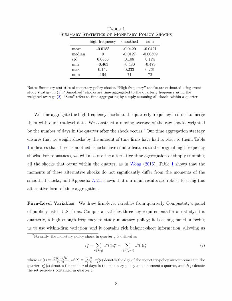
Table 1Summary Statistics of Monetary Policy Shocks

high frequency smoothed sum

mean -0.0185 -0.0429 -0.0421median 0 -0.0127 -0.00509std 0.0855 0.108 0.124min -0.463 -0.480 -0.479max 0.152 0.233 0.261num 164 71 72

Notes: Summary statistics of monetary policy shocks. “High frequency” shocks are estimated using eventstudy strategy in (1). “Smoothed” shocks are time aggregated to the quarterly frequency using theweighted average (2). “Sum” refers to time aggregating by simply summing all shocks within a quarter.

We time aggregate the high-frequency shocks to the quarterly frequency in order to merge

them with our firm-level data. We construct a moving average of the raw shocks weighted

by the number of days in the quarter after the shock occurs.7 Our time aggregation strategy

ensures that we weight shocks by the amount of time firms have had to react to them. Table

1 indicates that these “smoothed” shocks have similar features to the original high-frequency

shocks. For robustness, we will also use the alternative time aggregation of simply summing

all the shocks that occur within the quarter, as in Wong (2016). Table 1 shows that the

moments of these alternative shocks do not significantly differ from the moments of the

smoothed shocks, and Appendix A.2.1 shows that our main results are robust to using this

alternative form of time aggregation.

Firm-Level Variables We draw firm-level variables from quarterly Compustat, a panel

of publicly listed U.S. firms. Compustat satisfies three key requirements for our study: it is

quarterly, a high enough frequency to study monetary policy; it is a long panel, allowing

us to use within-firm variation; and it contains rich balance-sheet information, allowing us7Formally, the monetary-policy shock in quarter q is defined as

εmq =

∑t∈J(q)

ωa(t)εmt +

∑t∈J(q−1)

ωb(t)εmt (2)

where ωa(t) ≡ τnq (t)−τd

q (t)

τnq (t) , ωb(t) ≡ τd

q (t)

τnq (t) , τdq (t) denotes the day of the monetary-policy announcement in the

quarter, τnq (t) denotes the number of days in the monetary-policy announcement’s quarter, and J(q) denotethe set periods t contained in quarter q.

8

to construct our key variables of interest. To our knowledge, Compustat is the only U.S.

dataset that satisfies these three requirements. The main disadvantage of Compustat is that

it excludes privately held firms which are likely subject to more severe financial frictions.8

In Section 5, we calibrate our economic model to match a broad sample of firms, not just

those in Compustat.

Our main measure of investment is ∆ log kjt+1, where kjt+1 is the book value of the firm’s

tangible capital stock of firm j at the beginning of period t + 1. We use this log-difference

specification because investment is highly skewed, suggesting a log-linear rather than level-

linear regression specification. We use the net change in log capital rather than the log of

gross investment because gross investment often takes negative values.

We use three different measures of a firm’s financial position to proxy for default risk.

First, we measure leverage ℓjt as the firm’s debt-to-asset ratio, where debt is the sum of

short term and long term debt and assets is the book value of assets. Second, we measure

the firm’s credit rating crjt using S&P’s long-term issue rating of the firm. For most of the

paper, we will summarize the firm’s credit rating using an indicator variable for whether it

is at least an A rating, 1{crjt ≥ A}. Third, we measure the firm’s “distance to default” ddjt

following Gilchrist and Zakrajšek (2012). This measure uses the firm’s equity value to infer

its asset value; given the value of liabilities and assumptions on firm-level shocks, it then

backs out the implied probability of default. Distance to default ddjt has been shown by

Schaefer and Strebulaev (2008) to account well for variation in corporate bond prices due to

default risk and is widely used in the finance industry.

Appendix A.1 provides details of our data construction, which follows standard practice in

the investment literature. Panel (a) of Table 2 presents simple summary statistics of the final

sample used in our analysis. The mean capital growth rate is roughly 0.5% quarterly with

a standard deviation of 9.3%. The mean leverage ratio is approximately 27% with a cross-

sectional standard deviation of 36%. The mean distance to default implies a six standard8The main attractive alternatives, covering a much broader set of firm sizes than Compustat, are the

datasets constructed in Crouzet and Mehrotra (2017) (using data from the Quarterly Financial Reports)and in Dinlersoz et al. (2018a), (combining data from the U.S. Census Longitudinal Business Database,Orbis, and Compustat). However, the dataset in Crouzet and Mehrotra (2017) only follows small firms foreight quarters, which limits the ability to use within-firm variation, and the dataset in Dinlersoz et al. (2018a)contains data for small firms at an annual frequency.

9

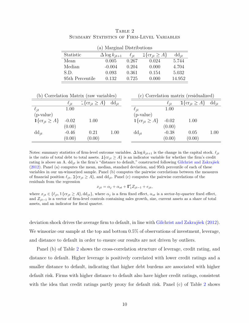
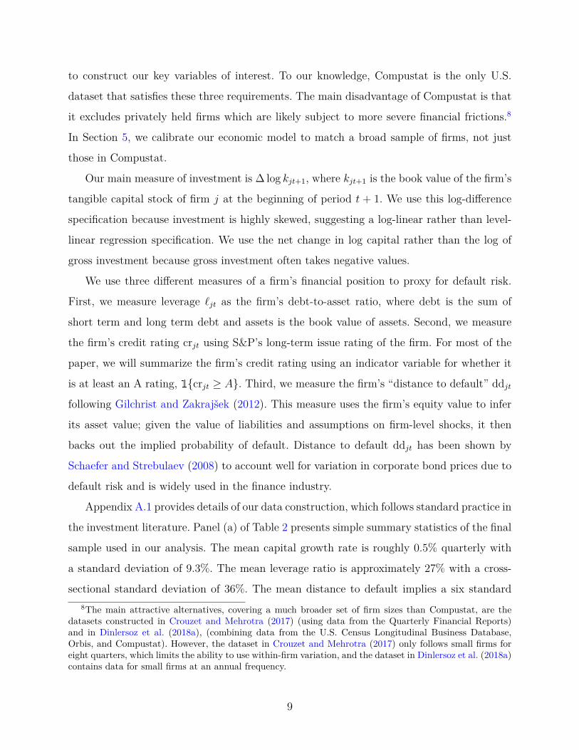
Table 2Summary Statistics of Firm-Level Variables

(a) Marginal DistributionsStatistic ∆ log kjt+1 ℓjt 1{crjt ≥ A} ddjt

Mean 0.005 0.267 0.024 5.744Median -0.004 0.204 0.000 4.704S.D. 0.093 0.361 0.154 5.03295th Percentile 0.132 0.725 0.000 14.952

(b) Correlation Matrix (raw variables) (c) Correlation matrix (residualized)ℓjt 1{crjt ≥ A} ddjt

ℓjt 1.00(p-value)1{crjt ≥ A} -0.02 1.00

(0.00)ddjt -0.46 0.21 1.00

(0.00) (0.00)

ℓjt 1{crjt ≥ A} ddjt

ℓjt 1.00(p-value)1{crjt ≥ A} -0.02 1.00

(0.00)ddjt -0.38 0.05 1.00

(0.00) (0.00)

Notes: summary statistics of firm-level outcome variables. ∆log kjt+1 is the change in the capital stock. ℓjtis the ratio of total debt to total assets. 1{crjt ≥ A} is an indicator variable for whether the firm’s creditrating is above an A. ddjt is the firm’s “distance to default,” constructed following Gilchrist and Zakrajšek(2012). Panel (a) computes the mean, median, standard deviation, and 95th percentile of each of thesevariables in our un-winsorized sample. Panel (b) computes the pairwise correlations between the measuresof financial position ℓjt, 1{crjt ≥ A}, and ddjt. Panel (c) computes the pairwise correlations of theresiduals from the regression

xjt = αj + αst + Γ′1Zjt−1 + ejt,

where xjt ∈ {ℓjt,1{crjt ≥ A},ddjt}, where αj is a firm fixed effect, αst is a sector-by-quarter fixed effect,and Zjt−1 is a vector of firm-level controls containing sales growth, size, current assets as a share of totalassets, and an indicator for fiscal quarter.

deviation shock drives the average firm to default, in line with Gilchrist and Zakrajšek (2012).

We winsorize our sample at the top and bottom 0.5% of observations of investment, leverage,

and distance to default in order to ensure our results are not driven by outliers.

Panel (b) of Table 2 shows the cross-correlation structure of leverage, credit rating, and

distance to default. Higher leverage is positively correlated with lower credit ratings and a

smaller distance to default, indicating that higher debt burdens are associated with higher

default risk. Firms with higher distance to default also have higher credit ratings, consistent

with the idea that credit ratings partly proxy for default risk. Panel (c) of Table 2 shows

10

that these results are all also true conditional on the controls in our baseline regression

specification (3) below.

2.2 Heterogeneous Responses to Monetary Policy

We estimate variants of the baseline empirical specification

∆ log kjt+1 = αj + αst + βxjt−1εmt + Γ′Zjt−1 + ejt, (3)

where αj is a firm j fixed effect, αst is a sector s by quarter t fixed effect, εmt is the monetary

policy shock, xjt ∈ {ℓjt,1{crjt ≥ A}, ddjt} is the firm’s leverage ratio, credit rating, or

distance to default, Zjt is a vector of firm-level controls, and ejt is a residual.9 Our main

coefficient of interest is β, which measures how the semi-elasticity of investment ∆ log kjt+1

with respect to monetary shocks εmt depends on the firm’s financial position xjt.10 This

coefficient estimate is conditional on a number of controls that may simultaneously affect

investment and leverage, but which are outside the scope of our economic model in Section

3. First, firm fixed effects αj capture permanent differences in investment behavior across

firms. Second, sector-by-quarter fixed effects αst capture differences in how broad sectors

are exposed to aggregate shocks. Finally, the firm-level controls Zjt include the level of the

financial position variable xjt−1, total assets, sales growth, current assets as a share of total

assets, and a fiscal quarter dummy. We cluster standard errors two ways in order to account

for correlation within firms and within quarters. This clustering strategy is conservative,

effectively leaving 71 time-series observations.

Table 3 reports the results from estimating the baseline specification (3). We perform two

normalizations to make the estimated coefficient β easily interpretable. First, we standardize

the firm’s leverage ℓjt and distance to default ddjt over the entire sample, so their units are

standard deviations relative to their mean value in our sample. Second, we normalize the9The sectors s we consider are: agriculture, forestry, and fishing; mining; construction; manufacturing;

transportation communications, electric, gas, and sanitary services; wholesale trade; retail trade; and services.We do not include finance, insurance, and real estate or public administration.

10We lag both financial position xjt−1 and the controls Zjt−1 to ensure they are predetermined at thetime of the monetary shock. Note that both kjt+1 and xjt measure end-of-period values. We denote theend-of-period capital stock with kjt+1 rather than kjt to be consistent with the standard notation in oureconomic model in Section 3.

11

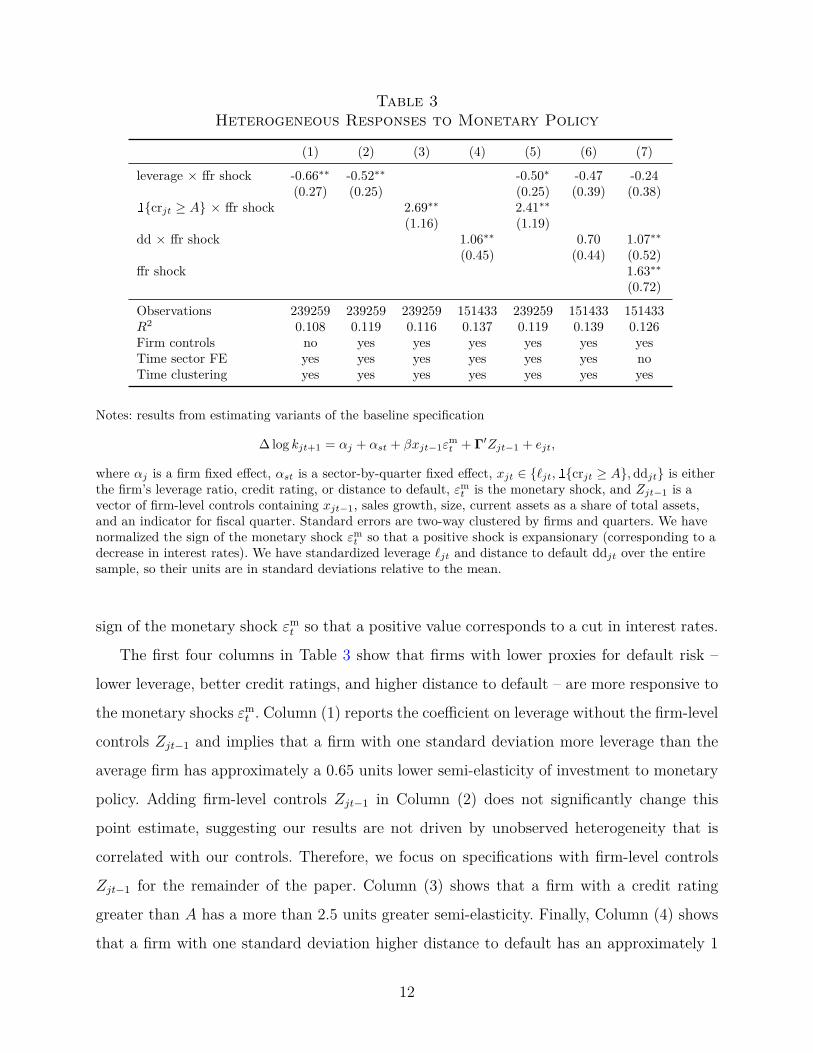
Table 3Heterogeneous Responses to Monetary Policy

(1) (2) (3) (4) (5) (6) (7)

leverage × ffr shock -0.66∗∗ -0.52∗∗ -0.50∗ -0.47 -0.24(0.27) (0.25) (0.25) (0.39) (0.38)

1{crjt ≥ A} × ffr shock 2.69∗∗ 2.41∗∗(1.16) (1.19)

dd × ffr shock 1.06∗∗ 0.70 1.07∗∗(0.45) (0.44) (0.52)

ffr shock 1.63∗∗(0.72)

Observations 239259 239259 239259 151433 239259 151433 151433R2 0.108 0.119 0.116 0.137 0.119 0.139 0.126Firm controls no yes yes yes yes yes yesTime sector FE yes yes yes yes yes yes noTime clustering yes yes yes yes yes yes yes

Notes: results from estimating variants of the baseline specification

∆log kjt+1 = αj + αst + βxjt−1εmt + Γ′Zjt−1 + ejt,

where αj is a firm fixed effect, αst is a sector-by-quarter fixed effect, xjt ∈ {ℓjt,1{crjt ≥ A},ddjt} is eitherthe firm’s leverage ratio, credit rating, or distance to default, εm

t is the monetary shock, and Zjt−1 is avector of firm-level controls containing xjt−1, sales growth, size, current assets as a share of total assets,and an indicator for fiscal quarter. Standard errors are two-way clustered by firms and quarters. We havenormalized the sign of the monetary shock εm

t so that a positive shock is expansionary (corresponding to adecrease in interest rates). We have standardized leverage ℓjt and distance to default ddjt over the entiresample, so their units are in standard deviations relative to the mean.

sign of the monetary shock εmt so that a positive value corresponds to a cut in interest rates.

The first four columns in Table 3 show that firms with lower proxies for default risk –

lower leverage, better credit ratings, and higher distance to default – are more responsive to

the monetary shocks εmt . Column (1) reports the coefficient on leverage without the firm-level

controls Zjt−1 and implies that a firm with one standard deviation more leverage than the

average firm has approximately a 0.65 units lower semi-elasticity of investment to monetary

policy. Adding firm-level controls Zjt−1 in Column (2) does not significantly change this

point estimate, suggesting our results are not driven by unobserved heterogeneity that is

correlated with our controls. Therefore, we focus on specifications with firm-level controls

Zjt−1 for the remainder of the paper. Column (3) shows that a firm with a credit rating

greater than A has a more than 2.5 units greater semi-elasticity. Finally, Column (4) shows

that a firm with one standard deviation higher distance to default has an approximately 1

12

unit higher semi-elasticity.11

Columns (5) and (6) in Table 3 show that these conclusions hold conditional on various

combinations of financial position, but statistical power falls due to the correlated nature

of the variables. Column (5) shows that jointly including leverage and credit rating only

slightly changes their interaction coefficients, consistent with their low correlation in Table

2. In contrast, Column (6) shows that the coefficients on both leverage and distance to default

become marginally insignificant once we jointly include both include leverage and distance

to default, consistent with their strong correlation in Table 2.

A natural way to assess the economic significance of our estimated interaction coefficients

β is to compare them to the average effect of a monetary policy shock. However, in our

baseline specification (3), the average effect is absorbed by the sector-by-quarter fixed effect

αst. We relax this restriction by estimating

∆ log kjt+1 = αj + γεmt + βxjt−1ε

mt + Γ′

1Zjt−1 + Γ′2Yt−1 + εjt, (4)

where Yt is a vector of aggregate controls for GDP growth, the inflation rate, and the unem-

ployment rate. Column (7) of Table 3 shows that the average investment semi-elasticity is

roughly 1.6.12 Hence, our interaction coefficients in the previous columns imply an econom-

ically meaningful degree of heterogeneity.

Within-Firm Variation In the economic model that we develop in Section 3, firms are

ex-ante homogeneous and heterogeneity in default risk is generated ex-post due to lifecycle

dynamics and idiosyncratic shocks. However, it is possible that the empirical results presented

in Table 3 are instead driven by permanent heterogeneity in how firms respond to monetary

policy according to their financial position xjt, breaking the tight link between default risk

and shock responsiveness in our model. In order to ensure our results are not driven by11A simple back of the envelope calculation using these estimates implies that monetary policy may

become substantially less effective in recessions. For example, average distance to default fell by 1.65 standarddeviations between 2007q2 and 2009q2; according to the estimates in Table 3, this change would decreasethe responsiveness of investment by 1.75 (holding all other covariates fixed).

12Assuming an annual depreciation rate of δ = 0.1, this estimated coefficient implies that a one percentagepoint cut in the interest rate increases annualized investment by 16%, in line with the upper end of estimateduser-cost elasticities in the literature, for example, Zwick and Mahon (2017).

13

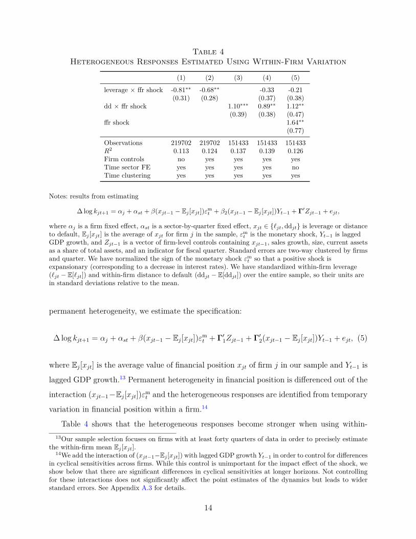
Table 4Heterogeneous Responses Estimated Using Within-Firm Variation

(1) (2) (3) (4) (5)

leverage × ffr shock -0.81∗∗ -0.68∗∗ -0.33 -0.21(0.31) (0.28) (0.37) (0.38)

dd × ffr shock 1.10∗∗∗ 0.89∗∗ 1.12∗∗(0.39) (0.38) (0.47)

ffr shock 1.64∗∗(0.77)

Observations 219702 219702 151433 151433 151433R2 0.113 0.124 0.137 0.139 0.126Firm controls no yes yes yes yesTime sector FE yes yes yes yes noTime clustering yes yes yes yes yes

Notes: results from estimating

∆log kjt+1 = αj + αst + β(xjt−1 − Ej [xjt])εmt + β2(xjt−1 − Ej [xjt])Yt−1 + Γ′Zjt−1 + ejt,

where αj is a firm fixed effect, αst is a sector-by-quarter fixed effect, xjt ∈ {ℓjt,ddjt} is leverage or distanceto default, Ej [xjt] is the average of xjt for firm j in the sample, εm

t is the monetary shock, Yt−1 is laggedGDP growth, and Zjt−1 is a vector of firm-level controls containing xjt−1, sales growth, size, current assetsas a share of total assets, and an indicator for fiscal quarter. Standard errors are two-way clustered by firmsand quarter. We have normalized the sign of the monetary shock εm

t so that a positive shock isexpansionary (corresponding to a decrease in interest rates). We have standardized within-firm leverage(ℓjt − E[ℓjt]) and within-firm distance to default (ddjt − E[ddjt]) over the entire sample, so their units arein standard deviations relative to the mean.

permanent heterogeneity, we estimate the specification:

∆ log kjt+1 = αj + αst + β(xjt−1 − Ej[xjt])εmt + Γ′

1Zjt−1 + Γ′2(xjt−1 − Ej[xjt])Yt−1 + ejt, (5)

where Ej[xjt] is the average value of financial position xjt of firm j in our sample and Yt−1 is

lagged GDP growth.13 Permanent heterogeneity in financial position is differenced out of the

interaction (xjt−1−Ej[xjt])εmt and the heterogeneous responses are identified from temporary

variation in financial position within a firm.14

Table 4 shows that the heterogeneous responses become stronger when using within-13Our sample selection focuses on firms with at least forty quarters of data in order to precisely estimate

the within-firm mean Ej [xjt].14We add the interaction of (xjt−1−Ej [xjt]) with lagged GDP growth Yt−1 in order to control for differences

in cyclical sensitivities across firms. While this control is unimportant for the impact effect of the shock, weshow below that there are significant differences in cyclical sensitivities at longer horizons. Not controllingfor these interactions does not significantly affect the point estimates of the dynamics but leads to widerstandard errors. See Appendix A.3 for details.

14

firm variation in financial position. We estimate the specification (5) only for leverage ℓjt

and distance to default ddjt because the within-firm variation in credit rating is small. We

standardize the demeaned variables (xjt − E[xjt]) so that their units are comparable to the

previous specification (3). Column (2) shows that a firm with a one standard deviation

within-firm increase in leverage has a 0.68 units lower semi-elasticity, compared to 0.52 in

the baseline specification (3). Column (3) shows that a firm with a one standard deviation

within-firm increase in distance to default has a 1.1 units higher semi-elasticity, compared

to 1.06 in the previous specification. Furthermore, Column (4) shows that controlling for

distance to default renders the coefficient on leverage insignificant. This result indicates that

the heterogeneous responses within-firm are primarily driven by distance to default, which

we view as our most direct measure of default risk.

Dynamics In order to estimate the dynamics of these differential responses across firms,we run the Jorda (2005)-style local projection of specification (5):

log kjt+h− log kjt = αjh+αsth+βh(xjt−1−Ej [xjt])εmt +Γ′

1hZjt−1+Γ′2h(xjt−1−Ej [xjt])Yt−1+ εjth,

(6)

where h ≥ 1 indexes the forecast horizon. The coefficient βh measures how the cumulative

response of investment in quarter t + h to a monetary policy shock in quarter t depends

on the firm’s financial position xjt in quarter t − 1. We estimate the local projection (6)

separately for demeaned leverage ℓjt and demeaned distance to default ddjt.

Figure 1 shows that firms with low leverage and high distance to default are consistently

more responsive to the shock up to three years after the shock. Panel (a) shows that the

peak of the differences by leverage occurs after four quarters and the differences disappear

after twelve quarters. Panel (b) shows that the differences by distance to default are larger

and significantly more persistent than for leverage. However, in both cases the long-run

differences are imprecisely estimated with large standard errors. We focus on the impact

effect of the shock for the rest of the paper because it is precisely estimated and is robust to

a broader set of modeling choices than are the dynamics.

Recent work by Jeenas (2018) performs a similar empirical exercise and argues that

low-leverage firms become significantly less responsive to monetary policy over time, in con-

15

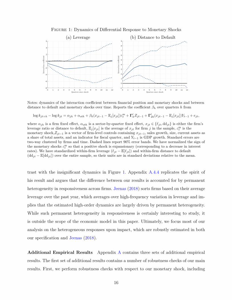
Figure 1: Dynamics of Differential Response to Monetary Shocks(a) Leverage (b) Distance to Default

0 1 2 3 4 5 6 7 8 9 10 11 12-8

-6

-4

-2

0

2

4

6

0 1 2 3 4 5 6 7 8 9 10 11 12-1

0

1

2

3

4

5

6

7

8

9

Notes: dynamics of the interaction coefficient between financial position and monetary shocks and betweendistance to default and monetary shocks over time. Reports the coefficient βh over quarters h from

log kjt+h − log kjt = αjh + αsth + βh(xjt−1 − Ej [xjt])εmt + Γ′

hZjt−1 + Γ′2h(xjt−1 − Ej [xjt])Yt−1 + ejt,

where αjh is a firm fixed effect, αsth is a sector-by-quarter fixed effect, xjt ∈ {ℓjt,ddjt} is either the firm’sleverage ratio or distance to default, Ej [xjt] is the average of xjt for firm j in the sample, εm

t is themonetary shock,Zjt−1 is a vector of firm-level controls containing xjt−1, sales growth, size, current assets asa share of total assets, and an indicator for fiscal quarter, and Yt−1 is GDP growth. Standard errors aretwo-way clustered by firms and time. Dashed lines report 90% error bands. We have normalized the sign ofthe monetary shocks εm

t so that a positive shock is expansionary (corresponding to a decrease in interestrates). We have standardized within-firm leverage (ℓjt − E[ℓjt]) and within-firm distance to default(ddjt − E[ddjt]) over the entire sample, so their units are in standard deviations relative to the mean.

trast with the insignificant dynamics in Figure 1. Appendix A.4.4 replicates the spirit of

his result and argues that the difference between our results is accounted for by permanent

heterogeneity in responsiveness across firms. Jeenas (2018) sorts firms based on their average

leverage over the past year, which averages over high-frequency variation in leverage and im-

plies that the estimated high-order dynamics are largely driven by permanent heterogeneity.

While such permanent heterogeneity in responsiveness is certainly interesting to study, it

is outside the scope of the economic model in this paper. Ultimately, we focus most of our

analysis on the heterogeneous responses upon impact, which are robustly estimated in both

our specification and Jeenas (2018).

Additional Empirical Results Appendix A contains three sets of additional empirical

results. The first set of additional results contains a number of robustness checks of our main

results. First, we perform robustness checks with respect to our monetary shock, including

16

but not limited to: controlling for the information channel of monetary policy using Green-

book forecast revisions (following Miranda-Agrippino and Ricco (2018)); using raw changes

in the Fed Funds rate rather than the shocks; and showing our results hold in the post-1994

sample. Second, we perform robustness checks regarding firm-level heterogeneity, including:

controlling for lagged investment; controlling for interactions of the monetary shock with

other firm-level covariates such as sales growth, future sales growth, size, or liquidity; and

investigating other indices of financial constraints.

The second set of results includes some additional analysis of the data. First, we show

that high-risk firms see a relative increase in their borrowing cost and a relative decrease

in their financing flows in response to a monetary expansion, consistent with our model.

Second, we show that the heterogeneous responses to monetary policy are primarily driven

by expansionary shocks. Third, we show that our results hold if we measure leverage using

only short term debt, only long term debt, other liabilities, or leverage net of liquid assets.

The third set of additional results relates our work to various strands of the existing

literature. First, we show that small firms, measured using Gertler and Gilchrist (1994)’s

methodology, are more responsive to monetary shocks in our sample; our results are robust

to controlling for this effect. Second, we show that older firms are slightly less responsive to

monetary shocks, consistent with recent work by Cloyne et al. (2018); again, our results are

robust to controlling for this effect. Third, we reconcile our results with recent work by Jeenas

(2018), as discussed above. We also show that our results are not driven by heterogeneity in

liquidity across firms; in fact, once we control for distance to default, we find that there are

no significant differences by liquidity in our specification (although statistical tests are weak

given the two variables are positively correlated).

3 Model

We now develop a heterogeneous firm New Keynesian model in order to interpret the cross-

sectional evidence in Section 2 and study aggregate implications. We describe the model in

three blocks: an investment block, which captures heterogeneous responses to monetary pol-

icy; a New Keynesian block, which generates a Phillips curve; and a representative household,

17

which closes the model.

3.1 Investment Block

The investment block contains a fixed mass of heterogeneous firms that invest in capital

subject to financial frictions. It builds heavily on the flexible-price model developed in Khan,

Senga and Thomas (2016). Besides incorporating sticky prices, we extend Khan, Senga and

Thomas (2016)’s framework in three additional ways. First, we add idiosyncratic capital qual-

ity shocks, which help us match observed default rates in the data. Second, we incorporate

aggregate adjustment costs in order to generate time-variation in the relative price of capital,

as in the financial accelerator literature (e.g., Bernanke, Gertler and Gilchrist (1999)). Third,

we assume that new entrants have lower initial productivity than incumbents, which helps

us match lifecycle dynamics.

Production firms Time is discrete and infinite. There is no aggregate uncertainty; in

Sections 4 and 6 below, we study the transition path in response to an unexpected monetary

shock. Each period, there is a fixed mass 1 of production firms.15 Each firm j ∈ [0, 1] produces

an undifferentiated good yjt using the production function

yjt = zjt(ωjtkjt)θlνjt, (7)

where zjt is an idiosyncratic total factor productivity shock, ωjt is an idiosyncratic capital

quality shock, kjt is the firm’s capital stock, ljt is the firm’s labor input, and θ+ ν < 1. The

idiosyncratic TFP shock follows an log-AR(1) process

log zjt+1 = ρzjt + εjt+1, where εjt+1 ∼ N(0, σ2). (8)

The capital quality shock is i.i.d. across firms and time and follows a truncated log-normal

process with support [−4σω, 0], where σω is the standard deviation of the underlying normal

distribution. This process implies that with some probability pω, no capital quality shock is

realized logωjt = 0 and with probability pω is drawn from the region of a normal distribution15We describe the entry and exit process below, which keeps the total mass of firms fixed.

18

within [−4σω, 0]. The capital quality shock also affects the value of the firm’s undepreciated

capital at the end of the period, (1−δ)ωjtkjt. We view the capital quality shocks as capturing

unmodeled forces which reduce the value of the firm’s capital, such as frictions in the resale

market, breakdown of machinery, or obsolescence of capital.16,17

The timing of events within period is as follows.

(i) Idiosyncratic shocks to TFP and capital quality are realized.

(ii) With probability πd the firm receives an i.i.d. exit shock and must exit the economy

after producing. Firms that do not receive the exit shock will be allowed to continue

into the next period.

(iii) The firm decides whether or not to default. If the firm defaults it immediately and

permanently exits the economy. In the event of default, lenders recover a fraction of

the firm’s capital stock (described in more detail below) and the remaining capital is

transferred lump-sum to the household. In order to continue, the firm must pay back

the face value of its outstanding debt, bjt, and pay a fixed operating cost ξ in units of

the final good.

(iv) Continuing firms produce using the production function (7). In order to produce, firms

hire labor ljt from a competitive labor market with real wage wt. Firms sell their output

to retailers (described below) in a competitive market at relative price pt. At this point,

firms that received the i.i.d. exit shock sell their undepreciated capital and exit the

economy.

(v) Continuing firms purchase new capital kjt+1 at relative price qt. Firms have two sources

of investment finance, each of which is subject to a friction. First, firms can issue new

nominal debt with real face value bjt+1 =Bjt+1

Πt+1, where Bjt+1 is the nominal face value

and Πt+1 is realized inflation on the final good (which is our numeraire, described16Mechanically, the capital quality shocks allow the model to generate positive default risk for a large

cross-section of firms. In our model, the value of a firm is dominated by the value of its undepreciated capitalstock; without risk to this stock, our model would have the counterfactual prediction that only firms withvery low net worth would have positive probability of default.

17Note that firms in our model face aggregate capital adjustment costs but not firm-level adjustment costs.We discuss the role of this assumption in determining our results in Footnote 27.

19

below).18 Lenders offer a price schedule Qt(zjt, kjt+1, bjt+1). The price schedule is de-

creasing in the amount of borrowing bjt+1 because firms may default on this borrowing

(we derive this price schedule below). Second, firms can use internal finance by lowering

dividend payments djt but cannot issue new equity, which bounds dividend payments

djt ≥ 0.19

We write the firm’s optimization problem recursively. The individual state variables of a

firm are its total factor productivity z and its net worth

n = maxl

ptz(ωk)θlν − wtl + qt(1− δ)ωk − b− ξ.

Net worth n is the total amount of resources available to the firm other than additional

borrowing. Conditional on continuing, the real equity value vt(z, n) solves the Bellman equa-

tion20

vt(z, n) = maxk′,b′

n− qtk′ +Qt(z, k

′, b′)b′ + Et

[Λt,t+1

(πdχ

1(n′)n′ + (1− πd)χ2t+1(z

′, n′)vt+1(z′, n′)}

)]such that n− qtk

′ +Qt(z, k′, b′)b′ ≥ 0 (9)

n′ = maxl′

pt+1z′(ω′k′)θ(l′)ν − wt+1l

′ + qt+1(1− δ)ω′k′ − b′

Πt+1

− ξ,

where χ1(n) and χ2t (z, n) are indicator variables for default conditional on the realization of

the exit shock.

Proposition 1. Consider a firm at time t that is eligible to continue into the next period, has

idiosyncratic productivity z, and has net worth n. The firm’s optimal decision is characterized18Note that all borrowing is short-term in our model; Footnote 26 argues that our main results are likely

to be robust to incorporating long-term debt.19The non-negative dividend constraint captures two key facts about external equity documented in the

corporate finance literature. First, firms face significant costs of issue new equity, both direct flotation costs(see, for example, Smith (1977)) and indirect costs (for example, Asquith and Mullins (1986)). Second, firmsissue external equity very infrequently (DeAngelo, DeAngelo and Stulz (2010)). The specific form of thenon-negativity constraint is widely used in the macro literature because it allows for efficient computationof the model in general equilibrium. Other potential assumptions include proportional costs of equity issues(e.g., Gomes, 2001; Cooley and Quadrini, 2001; Hennessy and Whited, 2005; Gilchrist, Sim and Zakrajsek,2014) and quadratic costs (e.g., Hennessy and Whited, 2007).

20Firms which receive the exogenous exit shock have simple decision rules. Those that do not default simplysell their undepreciated capital after production. Since these firms cannot borrow, they default whenever networth n < 0.

20

by one of the following three cases.

(i) Default: there exists a threshold nt(z) such that the firm defaults if n < nt(z).

(ii) Unconstrained: there exists a threshold nt(z) such that the firm is financiallyunconstrained if n > nt(z). Unconstrained firms follow the “frictionless” capital

accumulation policy k′t(z, n) = k∗

t (z). Unconstrained firms are indifferent over any

combination of b′ and d such that they remain unconstrained for every period with

probability one.

(iii) Constrained: firms with n ∈ [nt(z), nt(z)] are financially constrained. Con-

strained firms’ optimal investment k′t(z, n) and borrowing b′t(z, n) decisions solve the

Bellman equation (9). Constrained firms also pay zero dividends, which implies

qtk′ = n+Qt(z, k

′, b′)b′.

Proof. See Appendix B.1. ■

Proposition 1 characterizes the decision rules which solve this Bellman equation. Firms

with low net worth n < nt(z) default because they cannot satisfy the non-negativity con-

straint on dividends d ≥ 0. Firms with high net worth n > nt(z) are financially unconstrained

in the sense that they have no probability of default, which implies that any combination of

external financing b′ and internal financing d which leaves them unconstrained is optimal.

Finally, firms with net worth n ∈ [nt(z), nt(z)] are financially constrained in the sense that

they affected by default risk. These firms set d = 0 because the value of resources inside

the firm, used to lower borrowing costs, is higher than the value of resources outside the

firm. Over 99.4% of firms in our calibrated steady state are affected by default risk in this

way. Below, we focus our analysis on how these firms respond to monetary policy, since

the analysis of the unconstrained firms is fairly standard. It is important to note that these

constrained firms can be either risky constrained – have a positive probability of default in

the next period – or risk-free constrained – have no probability of default in the next period

yet not be financially unconstrained.

21

Lenders There is a representative financial intermediary that lends resources from the

representative household to firms at the firm-specific price schedule Qt(z, k′, b′). If the firm

defaults on the loan in the following period, the lender recovers a fraction α of the market

value of the firm’s capital stock qt+1ω′k′. The price schedule prices this default risk compet-

itively:

Qt(z, k′, b′) = Et

[Λt+1

(1

Πt+1−(πdχ

1(n′) + (1− πd)χ2t+1(z

′, n′))( 1

Πt+1−min{αqt+1(1− δ)ω′k′

b′/Πt+1, 1}))]

,

(10)

where n′ = maxl′ pt+1z(ω′k′)θ(l′)ν − wtl

′ + qt+1(1 − δ)ω′k′ − b′ − ξ is the net worth implied

by k′, b′, and the realization of z′. The debt price schedule does not depend on the capital

quality shock ωjt since capital quality is i.i.d.

Entry Each period, a mass µt of new firms enter the economy. We assume that the mass

of new entrants is equal to the mass of firms that exit the economy so that the total mass

of production firms is fixed in each period t. Each of these new entrants j ∈ [0, µt] draws a

idiosyncratic productivity zjt from the time-invariant distribution

µent(z) ∼ logN

(−m

σ√(1− ρ2)

,σ√

(1− ρ2)

),

where m ≥ 0 is a parameter. We calibrate m to match the average size and growth rates of

new entrants, motivated by the evidence in Foster, Haltiwanger and Syverson (2016) that

young firms have persistently low levels of measured productivity.21 New entrants also draw

capital quality from its ergodic distribution, are endowed with k0 units of capital from the

household, and have zero units of debt. They then proceed as incumbent firms.

3.2 New Keynesian Block

The New Keynesian block of the model is designed to parsimoniously generate a New Key-

nesian Phillips curve relating nominal variables to the real economy. Following Bernanke,21Foster, Haltiwanger and Syverson (2016) argue that these low levels of measured productivity among

young firms demand across firms rather than physical productivity. We remain agnostic about the interpre-tation of TFP in our model. Without the assumption that entrants have lower average productivity thanexisting firms, default risk would be disproportionately concentrated in a small group of young firms.

22

Gertler and Gilchrist (1999), we keep the nominal rigidities separate from the investment

block of the model.

Retailers and Final Good Producer There is a fixed mass of retailers i ∈ [0, 1]. Each

retailer producers a differentiated variety yit using the heterogeneous production firms’ good

as its only input:

yit = yit,

where yit is the amount of the undifferentiated good demanded by retailer i. Retailers

set a relative price for their variety pit but must pay a quadratic price adjustment costφ2

(pit

pit−1− 1)2

Yt, where Yt is the final good. The retailers’ demand curve is generated by the

representative final good producer, who has production function

Yt =

(∫y

γ−1γ

it di) γ

γ−1

,

where γ is the elasticity of substitution over intermediate goods. The final good is the nu-

meraire.

The retailers and final good producers aggregate into the familiar New Keynesian Phillips

Curve:

log Πt =γ − 1

φlog

ptp∗

+ βEt log Πt+1, (11)

where Πt is gross inflation of the final good and p∗ = γ−1γ

is the steady state relative price

of the heterogeneous production firm output.22 The Phillips Curve links the New Keynesian

block to the investment block through the relative price pt. When aggregate demand for

the final good Yt increases, retailers must increase production of their differentiated goods

because of the nominal rigidities; this force increases demand for the heterogeneous firms’

good yit, which increases its relative price pt and generates inflation through the Phillips

Curve (11).22We focus directly on the linearized formulation for computational simplicity.

23

Capital Good Producer There is a representative capital good producer who produces

aggregate capital Kt+1 using the technology

Kt+1 = Φ(ItKt

)Kt + (1− δ)Kt, (12)

where Φ( ItKt) = δ1/ϕ

1−1/ϕ

(ItKt

)1−1/ϕ

− δϕ−1

and It are units of the final good used to produce

capital.23 Profit maximization pins down the relative price of capital as

qt =1

Φ′( ItKt)=

(It/Kt

δ

)1/ϕ

. (13)

Monetary Authority The monetary authority sets the nominal risk-free interest rate

Rnomt according to the Taylor rule

logRnomt = log

1

β+ φπ log Πt + εm

t , where εmt ∼ N(0, σ2m),

where φπ is the weight on inflation in the reaction function, and εmt is the monetary policy

shock.

3.3 Representative Household and Equilibrium

There is a representative household with preferences over consumption Ct and labor supply

Lt represented by the expected utility function

E0

∞∑t

βt (logCt −ΨLt) ,

where β is the discount factor and Ψ controls the disutility of labor supply. The household

owns all firms in the economy. The stochastic discount factor and nominal interest rate are

linked through the Euler equation for bonds, Λt+1 =1

Rnomt /Πt+1

.

An equilibrium involves a set of value functions vt(z, n); decision rules k′t(z, n), b′t(z, n),

23We use external adjustment costs rather than internal adjustment costs for two reasons. First, externaladjustment costs generate time-variation in the price of capital, which allows us to study changes in therecovery value of capital. Second, because capital is liquid at the firm level, we can reduce the number ofindividual state variables, which is useful in the computation of the model.

24

lt(z, n); measure of firms µt(z, ω, k, b); debt price schedule Qt(z, k′, b′); and prices wt, qt, pt,

Πt, Λt,t+1 such that (i) all firms optimize, (ii) lenders price default risk competitively, (iii)

the household optimizes, (iii) the distribution of firms is consistent with decision rules, and

(iv) all markets clear. Appendix B.2 precisely defines an equilibrium of our model.

4 Channels of Monetary Transmission

Before performing the quantitative analysis, we theoretically characterize the channels through

which monetary policy affects investment in our model. This exercise identifies the key

sources of heterogeneous responses across firms, which motivates our calibration in Section

5.

Monetary policy experiment We study the effect an unexpected innovation to the

Taylor rule εmt followed by a perfect foresight transition back to steady state. This approach

allows for clean analytical results because there is no distinction between ex-ante expected

real interest rates and ex-post realized real interest rates. We focus on financially constrained

firms as defined in Proposition 1, which make up more than 99.4% of the firms in our

calibration.

Impact on decision rules The optimal choice of investment k′ and borrowing b′ satisfy

the following two conditions:

qtk′ = n+

1

Rt(z, k′, b′)b′ (14)(

qt − εR,k′(z, k′, b′)

b′

k′

)Rsp

t (z, k′, b′)

1− εR,b′(z, k′, b′)=

1

Rt

Et [MRPKt+1(z′, k′)] (15)

+1

Rt

Covt(MRPKt+1(z′, ω′k′), 1 + λt+1(z

′, ω′k′, b′))

Et[1 + λt+1(z′, ω′k′, b′))]

+1

Rt

Eω′

[v0t (zt+1(ω

′k′, b′))g(z(ω′k′, b′))

(∂zt+1(ω

′k′, b′)

∂k′ −∂zt+1(ω

′k′, b′)

∂b′

)],

where Rt is the risk-free rate between t and t + 1, Rt(z, k′, b′) = 1

Qt(z,k′,b′)is the firm’s

implied interest rate schedule, εRk′(z, k′, b′) is the elasticity of the interest rate schedule

25

with respect to investment k′, Rspt (z, k′, b′) = Rt(z, k

′, b′)/Rt is a measure of the borrowing

spread, εRb′(z, k′, b′) is the elasticity of the debt price schedule with respect to borrowing,

MRPKt+1(z, k′) = Eω′ [ ∂

∂k′(maxl′ pt+1z

′(ω′k′)θ(l′)ν −wt+1l′ + qt+1(1− δ)ω′k′)] is the return on

capital to the firm, λt(z, ωk, b) is the Lagrange multiplier on the non-negativity constraint on

dividends, (reflecting the shadow value of funds inside the firm relative to funds outside the

firm) and zt(ωk, b) is the default threshold in terms of productivity (which inverts the net

worth threshold defined in Proposition 1). Condition (14) is the non-negativity constraint on

dividends, which implies that capital expenditures qtk′ must be financed either by internal

resources n or new borrowing 1Rt(z,k′,b′)

b′. Condition (15) is the intertemporal Euler equation,

which equates the marginal cost of new capital k′ on the left-hand side with the marginal

benefit on on the right-hand side. The expectation and covariances in this expression are

only taken over the states in which the firm does not default.

The marginal cost of capital is the product of two terms. The first term, qt−εR,k′(z, k′, b′) b

′

k′,

is the relative price of new investment qt net of the interest savings due to higher capital,

εR,k′(z, k′, b′) b

′

k′. The interest savings result from the fact that, all else equal, higher capital

decreases expected losses due to default to the lenders. The second term in the marginal

cost of capital is related to borrowing costs, Rspt (z,k′,b′)

1−εR,b′ (z,k′,b′)

. Borrowing costs enter the marginal

cost of capital because borrowing is the marginal source of investment finance for these con-

strained firms. A higher interest rate spread or a higher slope of that spread result in higher

borrowing costs.

The marginal benefit of capital is the sum of three terms. The first term, 1RtEt [MRPKt+1(z

′, k′)],

is the expected return on capital discounted by the real interest rate.24 The second term,1Rt

Covt(MRPKt+1(z′,ω′k′),1+λt+1(z′,ω′k′,b′))Et[1+λt+1(z′,ω′k′,b′))]

, captures the covariance of the return on capital with

the firm’s shadow value of resources; capital is more valuable to the firm if it pays a high

return when the firm values additional resources. The third term captures how the additional

investment affects the firm’s default probabilities and, therefore, the value of the firm. In our

calibration, this term is negligible because the value of the firm close to the default threshold,

v0t (zt+1(ω′k′, b′)), is essentially zero.

Figure 2 plots the marginal benefit and marginal cost schedules as a function of capital24Firms discount using the risk-free rate because there is no aggregate risk.

26

Figure 2: Response to Monetary Policy for Risk-Free and Risky Firms(a) Risk-Free Firm (b) Risky Firm

Notes: Marginal benefit and cost curves as a function of capital investment k′ for firms with sameproductivity. Left panel is for a firm with high initial net worth and right panel is for a firm with low initialnet worth. Marginal cost curve is the left-hand side of (15) and marginal benefit left-hand side of (15).Dashed black lines plot the curves before the expansionary monetary policy shock, and solid blue lines plotthe curves after the shock.

accumulation k′. In order to illustrate the key economic mechanisms, we compare how these

curves shift following an expansionary monetary policy shock for two polar examples of firms.

These firms share the same level of productivity but differ in their initial net worth; the first

firm has high net worth and is currently risk-free (though it is still constrained in the sense

of Proposition 1), while the second has low net worth and is risky constrained.

Risk-Free Firm The left panel of Figure 2 plots the two schedules for the risk-free firm.

The marginal cost curve is flat when capital accumulation k′ can be financed without in-

curring default risk, but becomes upward sloping when the required creates default risk and

therefore a credit spread. The marginal benefit curve is downward sloping due to diminish-

ing returns of capital. In the initial equilibrium, the firm is risk-free because the two curves

intersect in the flat region of the marginal cost curve.

The expansionary monetary shock shifts both the marginal benefit and marginal cost

curves. The marginal benefit curves shifts out for two reasons. First, the shock decreases

the real interest rate, which decreases the firm’s discount rate Rt and therefore increases

the discounted return on capital. Second, the shock also changes the relative price of output

pt+1, the real wage wt+1, and the relative price of undepreciated capital qt+1 due to general

27

equilibrium. In our calibration, these changes increase the return on capital MRPKt+1(z, k′)

and therefore further shift out the marginal benefit curve. The shock also affects the covari-

ance term and the change in default threshold, which further shift out the marginal benefit

curve.

The marginal cost curve shifts up because the increase in aggregate investment demand

increases the relative price of capital qt. In the new equilibrium, the firm has increased its

investment and remains risk-free because the marginal benefit and marginal cost curves still

intersect along the flat region of marginal cost.

Risky Firm The right panel of Figure 2 plot how the marginal benefit and marginal cost

schedules shift for the risky firm. Because this firm has low initial net worth n, it needs

to borrow more than the risk-free firm to achieve the same level of investment. Hence, its

marginal cost curve is upward-sloping over a larger region of the state space.

The key difference between the risky and the risk-free firm is how monetary policy shifts

the marginal cost curve. As for the risk-free firm, the curve shifts up because the relative

price of capital qt increases, but there are now two additional effects. First, monetary policy

increases net worth n, which decreases the amount the firm needs to borrow to finance any

level of investment and therefore extends the flat region of the marginal cost curve. The

increase in net worth can be decomposed according to:

∂ log n

∂εmt

=1

1− ν − θ

(∂ log pt∂εm

t

− ν∂ logwt

∂εmt

)ιt(z, ωk)

n+

∂ log qt∂εm

t

qt(1− δ)ωk

n+

∂ log Πt

∂εmt

b/Πt

n,

(16)

where ιt(z, ωk) = maxl ptz(ωk)θlν −wtl. This expression (16) contains three ways that mon-

etary policy affects cash flows. First, monetary policy affects current revenues by changing

the relative price of output pt net of real labor costs νwt. Second, monetary policy affects the

value of firms’ undepreciated capital stock by changing the relative price of capital qt. Fi-

nally, monetary policy changes the real value of outstanding nominal debt through inflation

Πt.

The second key difference in how monetary policy affects the risky firm’s marginal cost

curve is that it flattens the upward-sloping region, reflecting reduced credit spreads. Credit

28

spreads fall because the expansionary shock decreases the expected losses from default to the

lender. Recall that, in the event of default, lenders recover αqt+1ωjt+1kjt+1 per unit of debt;

since the shock increases the relative price of capital qt+1, it also increases the recovery rate.

This channel is reminiscent of the “financial accelerator” in Bernanke, Gertler and Gilchrist

(1999). In addition, monetary policy also decreases the probability of default, although this

effect is quantitatively small in our calibration.

Whether the risky firm is more or less responsive than the risk-free firm depends crucially

on the size of these two shifts in the marginal cost curve. Theoretically, they may or may

not be large enough to induce the risky firm to be more responsive to monetary policy than

the risk-free firm. The goal of our calibration is to quantitatively discipline these shifts using

our model.25,26,27

Relationship to other papers The simple framework in Figure 2 provides a powerful

tool to organize various results in the existing literature.

(i) For example, Bernanke, Gertler and Gilchrist (1999) develop a model in which firms’

production functions are constant returns to scale, which results in a horizontal marginal

benefit curve for investment. The level of investment is determined by the point at

which this curve intersects the upward-sloping region of the marginal cost curve. There-

fore, monetary transmission is determined by how much the marginal cost curve re-25Appendix A.3.2 shows that the heterogeneous responses to monetary policy we find in the data are

primarily driven by expansionary shocks. While we do not emphasize that result in our model analysisdue to its wide standard errors, it is potentially consistent with the analysis in Figure 2. Suppose thathigh-risk firms tend to position themselves at the point where their marginal cost curve just begins to beupward sloping. Then an expansionary shock will move these firms forward along the upward-sloping part –dampening their response relative to low-risk firms – while a contractionary shock will move them backwardalong the flat part – not dampening their response.

26This analysis also suggests that our results are robust to incorporating long-term debt. In our model,high-risk firms are less responsive to monetary policy because they face an upward-sloping marginal costcurve for investment. This upward slope reflects the fact that the probability of default is increasing in theamount of borrowing the firm does. If we were to increase the maturity of debt but hold all other parametervalues fixed, then we would of course decrease default probabilities (since firms will have to roll over less debteach period) and potentially flatten out the marginal cost curve. However, we would also need to recalibratethe parameters in order to match the same average probability of default as in the current model. We expectthat this recalibration would also imply a similar slope of the default probabilities with respect to borrowingand, therefore, a similar slope for the marginal cost curve.

27This analysis can be extended to incorporate convex firm-level adjustment costs. These costs wouldinduce an upward-sloping marginal cost curve uniformly across firms, but risky firms would still face asteeper marginal cost curve due to their higher borrowing costs.

29

sponds to a monetary shock, which is primarily shifted due to the “financial accelerator”

channel described above.

(ii) Jeenas (2018) develops a model in which firms face a fixed cost of issuing debt but

can accumulate liquid financial assets. In response to a monetary shock, many firms

do not find it worthwhile to issue new debt, so their marginal source of investment

finance is liquid assets. This model implies a kinked marginal cost curve, which is flat

over the region that firms use their liquid assets but then vertical when the firm would

need to issue debt. Firms that have more liquid assets have a larger flat region of their

marginal cost curve and are therefore more responsive to monetary policy.

(iii) Cloyne et al. (2018) argue that young firms are more responsive to monetary shocks

in the U.S. and the U.K. While we show in Appendix A.4.2 that age does not drive

our empirical results, one can nevertheless interpret their findings through the lens

of our model. One possible interpretation is that young firms face a steeper marginal

cost curve than old firms, but young firms’ marginal cost curve is also more sensitive

to monetary policy. Another interpretation is that the young firms’ marginal benefit

curve is itself more responsive to monetary policy, for example if their product demand

is more cyclically sensitive.

5 Parameterization

We now calibrate the model and verify that its steady state behavior is consistent with key

features of the micro data. In Section 6, we use the calibrated model to quantitatively study

the effect of a monetary policy shock εmt .

5.1 Calibration

We calibrate the model in two steps. First, we exogenously fix a subset of parameters. Second,

we choose the remaining parameters in order to match moments in the data.

30

Table 5Fixed Parameters

Parameter Description ValueHouseholdβ Discount factor 0.99Firmsν Labor coefficient 0.64θ Capital coefficient 0.21δ Depreciation 0.025New Keynesian Blockϕ Aggregate capital AC 4γ Demand elasticity 10φπ Taylor rule coefficient 1.25φ Price adjustment cost 90

Notes: Parameters exogenously fixed in the calibration.

Fixed Parameters Table 5 lists the parameters that we fix. The model period is one

quarter, so we set the discount factor β = 0.99. We set the coefficient on labor ν = 0.64. We

choose the coefficient on capital θ = 0.21 to imply a total returns to scale of 85%. Capital

depreciates at rate δ = 0.025 quarterly. We choose the elasticity of substitution in final goods

production γ = 10, implying a steady state markup of 11%. This choice implies that the

steady state labor share is γ−1γν ≈ 58%, close to the current U.S. labor share reported in

Karabarbounis and Neiman (2013). We choose the coefficient on inflation in the Taylor rule

φπ = 1.25, in the middle of the range commonly considered in the literature. We set the

price adjustment cost parameter φ = 90 to generate the slope of the Phillips Curve equal to

0.1, as in Kaplan, Moll and Violante (2017). Finally, we set the curvature of the aggregate

adjustment costs φ = 2.5 in order to roughly match the peak response of investment relative

to the peak response of output estimated in Christiano, Eichenbaum and Evans (2005).

Fitted Parameters We choose the parameters listed in Table 6 to match the empirical

moments reported in Table 7.28 The first set of parameters govern the idiosyncratic shocks: ρ

and σ control the AR(1) process for TFP and σω controls the i.i.d. process for capital quality.28We exogenously fix the persistence of productivity shocks to ρ = 0.9 due to Clementi and Palazzo

(2015)’s result that the persistence and volatility of an AR(1) is hard to separately identify from investmentdata.

31

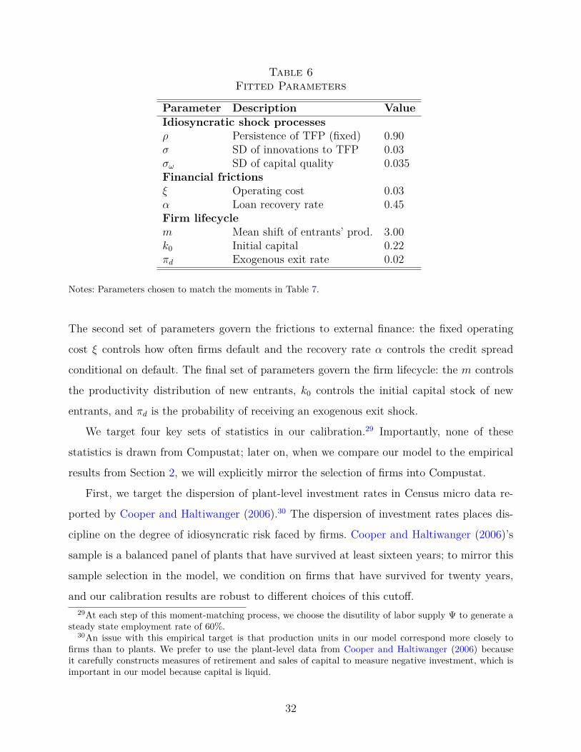
Table 6Fitted Parameters

Parameter Description ValueIdiosyncratic shock processesρ Persistence of TFP (fixed) 0.90σ SD of innovations to TFP 0.03σω SD of capital quality 0.035Financial frictionsξ Operating cost 0.03α Loan recovery rate 0.45Firm lifecyclem Mean shift of entrants’ prod. 3.00k0 Initial capital 0.22πd Exogenous exit rate 0.02

Notes: Parameters chosen to match the moments in Table 7.

The second set of parameters govern the frictions to external finance: the fixed operating

cost ξ controls how often firms default and the recovery rate α controls the credit spread

conditional on default. The final set of parameters govern the firm lifecycle: the m controls

the productivity distribution of new entrants, k0 controls the initial capital stock of new

entrants, and πd is the probability of receiving an exogenous exit shock.

We target four key sets of statistics in our calibration.29 Importantly, none of these

statistics is drawn from Compustat; later on, when we compare our model to the empirical

results from Section 2, we will explicitly mirror the selection of firms into Compustat.

First, we target the dispersion of plant-level investment rates in Census micro data re-

ported by Cooper and Haltiwanger (2006).30 The dispersion of investment rates places dis-

cipline on the degree of idiosyncratic risk faced by firms. Cooper and Haltiwanger (2006)’s

sample is a balanced panel of plants that have survived at least sixteen years; to mirror this

sample selection in the model, we condition on firms that have survived for twenty years,

and our calibration results are robust to different choices of this cutoff.29At each step of this moment-matching process, we choose the disutility of labor supply Ψ to generate a

steady state employment rate of 60%.30An issue with this empirical target is that production units in our model correspond more closely to

firms than to plants. We prefer to use the plant-level data from Cooper and Haltiwanger (2006) becauseit carefully constructs measures of retirement and sales of capital to measure negative investment, which isimportant in our model because capital is liquid.

32

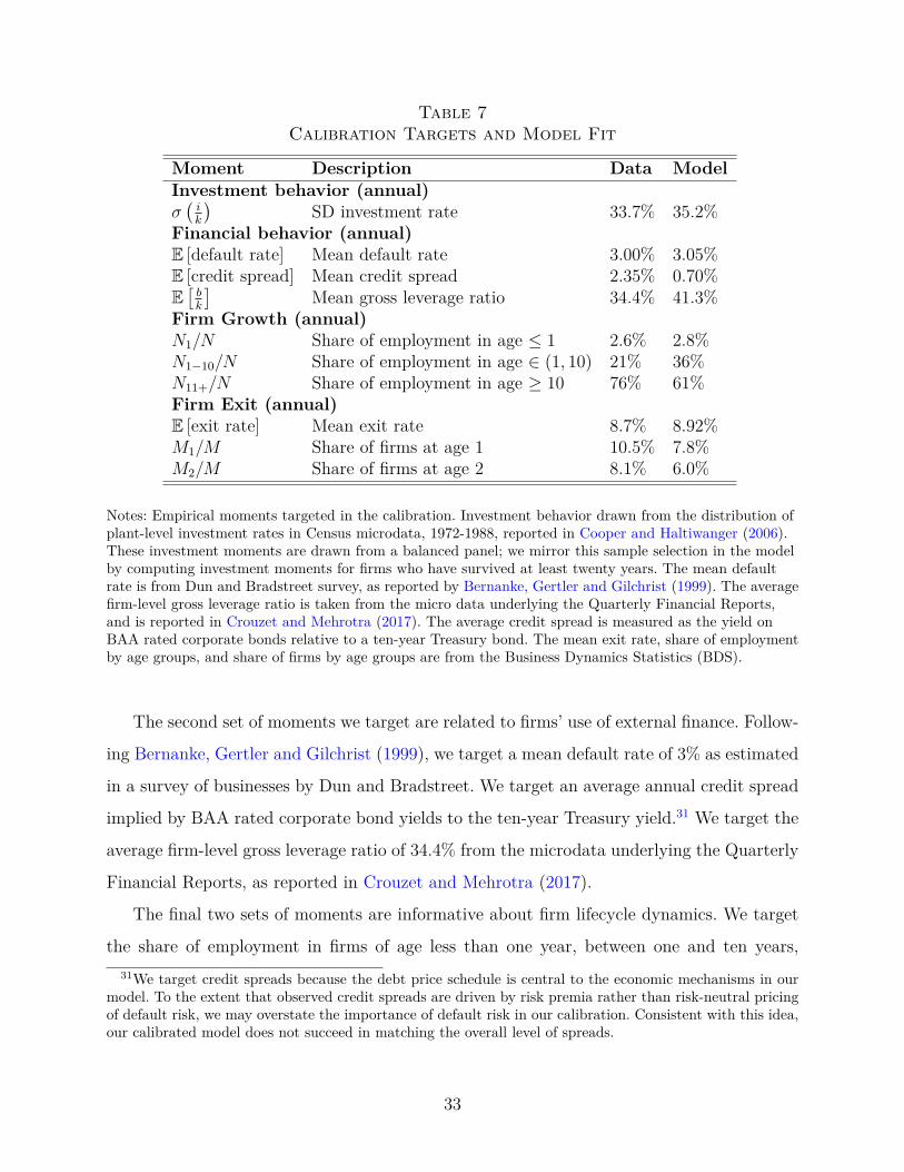
Table 7Calibration Targets and Model Fit

Moment Description Data ModelInvestment behavior (annual)σ(ik

)SD investment rate 33.7% 35.2%

Financial behavior (annual)E [default rate] Mean default rate 3.00% 3.05%E [credit spread] Mean credit spread 2.35% 0.70%E[bk

]Mean gross leverage ratio 34.4% 41.3%

Firm Growth (annual)N1/N Share of employment in age ≤ 1 2.6% 2.8%N1−10/N Share of employment in age ∈ (1, 10) 21% 36%N11+/N Share of employment in age ≥ 10 76% 61%Firm Exit (annual)E [exit rate] Mean exit rate 8.7% 8.92%M1/M Share of firms at age 1 10.5% 7.8%M2/M Share of firms at age 2 8.1% 6.0%

Notes: Empirical moments targeted in the calibration. Investment behavior drawn from the distribution ofplant-level investment rates in Census microdata, 1972-1988, reported in Cooper and Haltiwanger (2006).These investment moments are drawn from a balanced panel; we mirror this sample selection in the modelby computing investment moments for firms who have survived at least twenty years. The mean defaultrate is from Dun and Bradstreet survey, as reported by Bernanke, Gertler and Gilchrist (1999). The averagefirm-level gross leverage ratio is taken from the micro data underlying the Quarterly Financial Reports,and is reported in Crouzet and Mehrotra (2017). The average credit spread is measured as the yield onBAA rated corporate bonds relative to a ten-year Treasury bond. The mean exit rate, share of employmentby age groups, and share of firms by age groups are from the Business Dynamics Statistics (BDS).

The second set of moments we target are related to firms’ use of external finance. Follow-

ing Bernanke, Gertler and Gilchrist (1999), we target a mean default rate of 3% as estimated

in a survey of businesses by Dun and Bradstreet. We target an average annual credit spread

implied by BAA rated corporate bond yields to the ten-year Treasury yield.31 We target the

average firm-level gross leverage ratio of 34.4% from the microdata underlying the Quarterly

Financial Reports, as reported in Crouzet and Mehrotra (2017).

The final two sets of moments are informative about firm lifecycle dynamics. We target

the share of employment in firms of age less than one year, between one and ten years,31We target credit spreads because the debt price schedule is central to the economic mechanisms in our

model. To the extent that observed credit spreads are driven by risk premia rather than risk-neutral pricingof default risk, we may overstate the importance of default risk in our calibration. Consistent with this idea,our calibrated model does not succeed in matching the overall level of spreads.

33

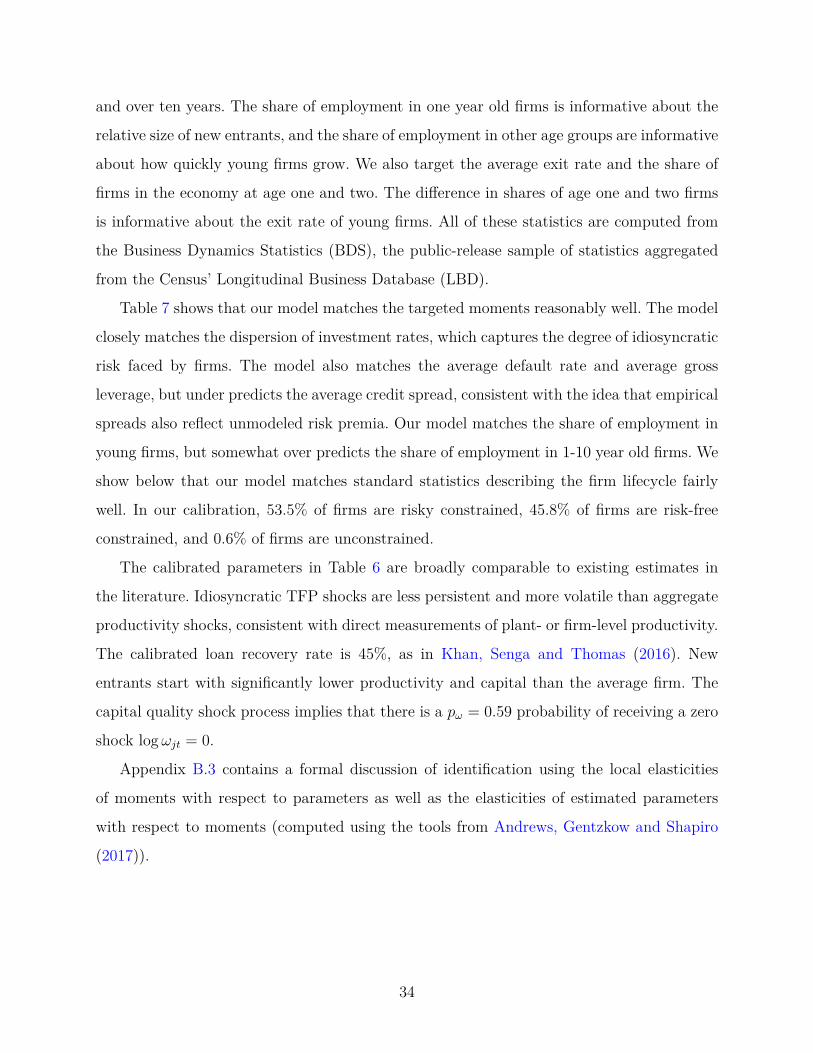
and over ten years. The share of employment in one year old firms is informative about the

relative size of new entrants, and the share of employment in other age groups are informative

about how quickly young firms grow. We also target the average exit rate and the share of

firms in the economy at age one and two. The difference in shares of age one and two firms

is informative about the exit rate of young firms. All of these statistics are computed from

the Business Dynamics Statistics (BDS), the public-release sample of statistics aggregated

from the Census’ Longitudinal Business Database (LBD).

Table 7 shows that our model matches the targeted moments reasonably well. The model

closely matches the dispersion of investment rates, which captures the degree of idiosyncratic

risk faced by firms. The model also matches the average default rate and average gross

leverage, but under predicts the average credit spread, consistent with the idea that empirical

spreads also reflect unmodeled risk premia. Our model matches the share of employment in

young firms, but somewhat over predicts the share of employment in 1-10 year old firms. We

show below that our model matches standard statistics describing the firm lifecycle fairly

well. In our calibration, 53.5% of firms are risky constrained, 45.8% of firms are risk-free

constrained, and 0.6% of firms are unconstrained.

The calibrated parameters in Table 6 are broadly comparable to existing estimates in

the literature. Idiosyncratic TFP shocks are less persistent and more volatile than aggregate

productivity shocks, consistent with direct measurements of plant- or firm-level productivity.

The calibrated loan recovery rate is 45%, as in Khan, Senga and Thomas (2016). New

entrants start with significantly lower productivity and capital than the average firm. The

capital quality shock process implies that there is a pω = 0.59 probability of receiving a zero

shock logωjt = 0.

Appendix B.3 contains a formal discussion of identification using the local elasticities

of moments with respect to parameters as well as the elasticities of estimated parameters

with respect to moments (computed using the tools from Andrews, Gentzkow and Shapiro

(2017)).

34

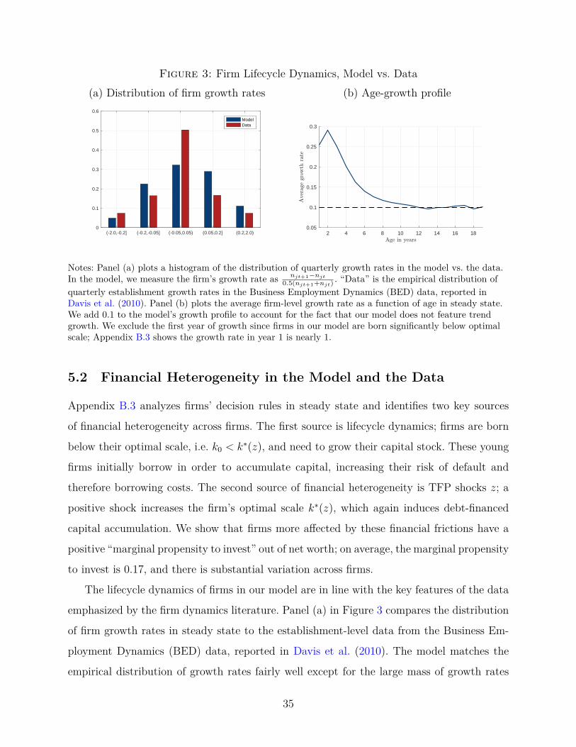
Figure 3: Firm Lifecycle Dynamics, Model vs. Data(a) Distribution of firm growth rates (b) Age-growth profile

(-2.0,-0.2] (-0.2,-0.05] (-0.05,0.05) (0.05,0.2] (0.2,2.0)0

0.1

0.2

0.3

0.4

0.5

0.6

ModelData

2 4 6 8 10 12 14 16 180.05

0.1

0.15

0.2

0.25

0.3

Notes: Panel (a) plots a histogram of the distribution of quarterly growth rates in the model vs. the data.In the model, we measure the firm’s growth rate as njt+1−njt

0.5(njt+1+njt). “Data” is the empirical distribution of

quarterly establishment growth rates in the Business Employment Dynamics (BED) data, reported inDavis et al. (2010). Panel (b) plots the average firm-level growth rate as a function of age in steady state.We add 0.1 to the model’s growth profile to account for the fact that our model does not feature trendgrowth. We exclude the first year of growth since firms in our model are born significantly below optimalscale; Appendix B.3 shows the growth rate in year 1 is nearly 1.

5.2 Financial Heterogeneity in the Model and the Data

Appendix B.3 analyzes firms’ decision rules in steady state and identifies two key sources

of financial heterogeneity across firms. The first source is lifecycle dynamics; firms are born

below their optimal scale, i.e. k0 < k∗(z), and need to grow their capital stock. These young

firms initially borrow in order to accumulate capital, increasing their risk of default and

therefore borrowing costs. The second source of financial heterogeneity is TFP shocks z; a

positive shock increases the firm’s optimal scale k∗(z), which again induces debt-financed

capital accumulation. We show that firms more affected by these financial frictions have a

positive “marginal propensity to invest” out of net worth; on average, the marginal propensity

to invest is 0.17, and there is substantial variation across firms.

The lifecycle dynamics of firms in our model are in line with the key features of the data

emphasized by the firm dynamics literature. Panel (a) in Figure 3 compares the distribution

of firm growth rates in steady state to the establishment-level data from the Business Em-

ployment Dynamics (BED) data, reported in Davis et al. (2010). The model matches the

empirical distribution of growth rates fairly well except for the large mass of growth rates

35

within (−0.05, 0.05) in the data. This discrepancy is driven by the fact that 15% of firms

have exactly zero growth rates in the data; these observations likely correspond to small,

non-growing establishments, which are outside our model. Panel (b) in Figure 3 shows that

the model produces a negative correlation of age and growth, as in the data (and comparable

to the model in Clementi and Palazzo (2015)).32

Appendix B.3 further analyzes the behavior of the model in steady state and compares it

to the data. First, we further analyze the lifecycle dynamics of firms. Second, we show that

the joint distribution of investment and leverage rates in our model is comparable to Census

and Compustat data. Third, we show that measured investment-cash flow sensitivities in our

model are roughly in line with the data. Finally, we compare our model’s sample of public

vs. private firms (used to replicate the empirical results in Section 6) to the data.

6 Quantitative Monetary Policy Analysis

We now quantitatively analyze the effect of a monetary policy shock εmt . Section 6.1 begins

the analysis by computing the aggregate impulse responses to an expansionary shock in

our calibrated model. Section 6.2 then studies the heterogeneous effects of monetary policy

across firms and shows that, consistent with the empirical results from Section 2, firms with

high default risk are less responsive to monetary policy. Finally, Section 6.3 shows that the

aggregate effect of monetary policy depends on the distribution of default risk across firms.

The economy is initially in steady state and unexpectedly receives a εm0 = −0.0025

innovation to the Taylor rule which reverts to 0 according to εmt+1 = ρmε

mt with ρm = 0.5. We

compute the perfect foresight transition path of the economy as it converges back to steady

state.33

32We exclude the growth of firms less than one year old from this comparison because their growth rate isdominated by the fact that all firms start with low initial capital k0; the average growth rate of these firmsis nearly 1. We exclude them from the figure since they account for a small share of economic activity butwould dominate the scaling.

33Allowing for persistence in the monetary policy shocks themselves is a simple way to create inertia inresponse to a monetary shock; in the representative firm version of the model, the response is very similarto a version of the model in which the innovations are transitory but the Taylor rule includes interest ratesmoothing.

36

Figure 4: Aggregate Responses to Expansionary Monetary Shock

2 4 6 8 10Quarters

-0.8

-0.6

-0.4

-0.2

0

0.2

0.4

0.6Annualizedp.p.deviation

Interest Rates and Inflation

Real rate

Inflation

Nominal rate

2 4 6 8 10Quarters

-0.2

0

0.2

0.4

0.6

0.8

1

1.2

%deviation

Aggregate Quantities

Output

Consumption

Investment

2 4 6 8 10Quarters

-0.1

0

0.1

0.2

0.3

0.4

0.5

0.6

%deviation

Prices

Intermediate Good Price

Capital Price

Real Wage

Notes: Aggregate impulse responses to a εm0 = −0.0025 innovation to the Taylor rule which decays at rate

ρm = 0.5. Computed as the perfect foresight transition in response to a series of unexpected innovationsstarting from steady state.

6.1 Aggregate Response to Monetary Policy

Figure 4 plots the responses of key aggregate variables to this expansionary shock. The shock

lowers the nominal interest rate and, because prices are sticky, also lowers the real interest

rate. The lower real interest rate stimulates investment demand by shifting out the marginal

benefit of investment, as discussed in Section 4. It also stimulates consumption demand

from the household due to the standard intertemporal substitution. The higher aggregate

demand for goods changes other prices in the economy, further shifting the marginal benefit

and marginal costs curves for investment. Overall, investment increases by approximately

1.1%, consumption increases by 0.35%, and output increases by 0.4%. These magnitudes are

broadly in line with the peak effect of monetary policy estimated in Christiano, Eichenbaum

and Evans (2005).34

34Our model does not generate the hump-shaped aggregate responses emphasized by Christiano, Eichen-baum and Evans (2005). We could do so by incorporating adjustment costs to investment rather than capital.However, in order to be consistent with the hump-shaped responses of consumption and employment, wewould also need to add habit formation and potentially labor adjustment costs. While interesting, this ex-tension is outside the scope of this paper, whose goal is to focus on the role of financial heterogeneity inmonetary transmission using an otherwise basic New Keynesian model.

37

6.2 Heterogeneous Responses to Monetary Policy

We now study the heterogeneous responses to monetary policy across firms in our model

and show that they are consistent with the data. We also decomposes the various channels

through which monetary policy affects investment.

Model-Implied Regression Coefficients In order to directly compare our model to the

data, we simulate a panel of firms in response to a monetary shock and estimate our empirical

specification (5) on the simulated data:35

∆ log kjt+1 = αj + αst + β(xjt−1 − Ej[xjt])εmt + Γ′

1Zjt−1 + Γ′2(xjt−1 − Ej[xjt])Yt−1 + ejt.

We mirror the sample selection into Compustat by conditioning on firms that have survived

at least ten years, which is on the upper end of time to IPO reported in Wilmer et al. (2017).

Appendix B.3 shows that the behavior of the model’s public firms vs. private firms compares

fairly well to the data along certain dimensions. We assume that the high-frequency shocks

εmt we measure in the data are the innovations to the Taylor rule in the model.36 We estimate

the regressions using data from one year before the shock to ten quarters after the shock.

We estimate the specification (5) using leverage ℓjt as the measure of financial position

xjt. We use leverage ℓjt for two reasons. First, it is not obvious how to compute our other

measures of financial position in the model; in the data, credit ratings are constructed by

ratings agencies – which do not exist in our model – and distance to default is based on

the volatility of firms’ equity values – which are partially determined by aggregate shocks.

Second, there is a tight relationship between leverage and default risk in the model. This

relationship occurs because there is a monotonic relationship between leverage and net worth

(shown in Figure 24 in Appendix B.3), and firms only default when net worth falls below35In the model, we use time fixed effects rather than sector-time fixed effects. In addition, we do include

the subset of the controls in Zjt which are not in our model.36In our model, the change in the nominal interest rate is smaller than the innovation to the Taylor rule

because the monetary authority responds to the resulting inflation. This fact may lead to an inconsistencybetween the monetary shocks in the model and the measured shocks in the data, which are based on changesin expected nominal rates. Our implicit assumption is that the feedback effect through the Taylor rule takessufficient time that it is not incorporated into the measure of the high-frequency shocks. Because we use theone-month futures, our assumption requires that the monetary authority respond to inflation with at mosta one month lag.

38

Table 8Empirical results, model vs. data

LHS: ∆ log kjt LHS: ∆rjtData Model Data Model(1) (2) (3) (4)

demeaned leverage × ffr shock −0.68∗∗ −0.59 0.17∗∗ 0.26(0.28) (0.06)

Firm controls yes yes yes yesTime FE yes yes yes yesR2 0.12 0.58 0.55 0.99

Notes: Results from running the specification ∆log kjt = αj + αt + β(ℓjt−1 − Ej [ℓjt])εmt + Γ′Zjt−1 + ejt on

model-simulated data, where αj is a firm fixed effect, αst is a sector-by-quarter fixed effect, ℓjt−1 is thefirm’s leverage, εm

t is the monetary shock, Zjt−1 is a vector of firm-level controls containing leverage, cashflow, and size, and Ej [ℓjt] is the average leverage of firm j in our sample. We have normalized the sign ofthe monetary shock εm

t so that a positive shock is expansionary (corresponding to a decrease in interestrates). We have standardized leverage ℓjt or demeaned leverage ℓjt − Ej [ℓjt] over the entire sample, so itsunits are in standard deviations relative to the mean. In the model, the sample period is four quartersbefore the monetary shock through ten quarters after the shock. To mirror the sample selection intoCompustat, we condition on firms that have survived at least ten years. Columns (3) and (4) replace theleft-hand side variable with ∆rjt. In the model, ∆rjt is the change in the firm’s interest rate 1/Qjt. In thedata, ∆rjt is the change in the firm’s total interest payments over twelve quarters divided by totalliabilities. We compute the change over twelve quarters because the data’s interest rate measures averagecosts over all borrowing, and the average maturity of corporate debt is roughly three years. See AppendixA.3.1 for the full dynamics.

the default threshold n(z).

Table 8 shows that high-leverage firms are less responsive to monetary policy in the

model, as in the data. In the data, a firm with one standard deviation more leverage than

the average firm has an investment semi-elasticity that is approximately −0.7 percentage

points lower than the average firm; in the model, that firm is has an approximately −0.6

lower semi-elasticity, which is well within one standard error of the data. The R2 of the

regression is higher in the data than in the model, indicating that the data contain more

unexplained variation in investment.

Figure 5 shows that the dynamics of the differential responses of investment are are per-

sistent in the model, consistent with the data. In this figure, we estimate the local projection

(6) on our model-simulated data. Quantitatively, the model’s differences stay within the

data’s 90% confidence interval up to eight quarters after the shock.

These heterogeneous responses indicate that high-leverage firms are positioned on the

39

Figure 5: Dynamics of differential responses, model vs. data

0 1 2 3 4 5 6 7Quarters since shock

-6

-5

-4

-3

-2

-1

0

1

2

Interactioncoeffi

cient

Data

Model

Notes: dynamics of the interaction coefficient between leverage and monetary shocks and between distanceto default and monetary shocks over time. Reports the coefficient βh over quarters h from

log kjt+h − log kjt = αjh + αsth + βh(xjt−1 − Ej [xjt])εmt + Γ′

hZjt−1 + Γ′2h(xjt−1 − Ej [xjt])Yt−1 + ejt,

where αj is a firm fixed effect, αst is a sector-by-quarter fixed effect, ℓjt−1 is the firm’s leverage, εmt is the

monetary shock, Zjt−1 is a vector of firm-level controls containing leverage, cash flow, and size, and Ej [ℓjt]is the average leverage of firm j in our sample. We have normalized the sign of the monetary shock εm

t sothat a positive shock is expansionary (corresponding to a decrease in interest rates). We have standardizedleverage ℓjt or demeaned leverage ℓjt − Ej [ℓjt] over the entire sample, so its units are in standarddeviations relative to the mean. In the model, the sample period is four quarters before the monetary shockthrough ten quarters after the shock. To mirror the sample selection into Compustat, we condition on firmsthat have survived at least ten years.

upward-sloping part of their marginal cost curve from Figure 2, and that the shifts in that

curve are quantitatively dominated by the shift out in the marginal benefit curve. An im-

plication of this mechanism is that firms with high leverage should see a larger increase in

their interest rate 1/Qjt in response to the monetary shock. Columns (3) and (4) in Table 8

show that this implication holds true in both the model and in the data. In these columns,

we replace the left-hand side of the empirical specification (5) with the change in the firm’s

interest rate and find that it increases more for high-leverage firms. Appendix A.3 further

studies heterogeneous responses of firm-level interest rates in the data.37

37We do not study the response of interest rates in Section 2 because our measure of interest rates is totalinterest payments divided by total liabilities. This variable is a noisy measure of the firm’s interest rate ona marginal unit of borrowing, so the results are subject to large standard errors.

40

Figure 6: Decomposition of Semi-Elasticity of Capital to Monetary Policy Shock

0.5 1 1.5 2 2.5 3 3.5 4 4.5 5Net worth

-15

-10

-5

0

5

10

Sem

i-Elasticity

0.02

0.03

0.04

0.05

0.06

0.07

0.08

0.09

0.1

0.11

Mas

s of

firm

s

Average Semi-Elasticity w.r.t. Monetary Shock

Real rate only

Capital price only

Others

Notes: Semi-elasticity of capital in response to monetary shock and the initial distribution of firms. “Realrate only” refers to feeding in the path of the real interest rate Rt but keeping all other prices fixed atsteady state. “Capital price only” refers to feeding in the path of the relative price of capital qt but keepingall other prices fixed at steady state. “Others” refers to feeding in all other prices but keeping the real rateand capital price fixed at steady state. Dashed purple line is the initial distribution of firms. Idiosyncraticproductivity shocks z have been averaged over using their ergodic distribution.

Decomposition of Channels Driving Heterogeneous Responses In order to better

understand the sources of these heterogeneous responses across firms, we now decompose

the channels through which monetary policy affects firms’ investment intro three different

channels. First, we compute the “direct effect” of monetary policy by feeding in the path of

the real interest rate Rt and hold all other prices fixed at steady state. Second, we feed in

the series of the relative price of capital qt but keep all other prices fixed. Finally, we feed in

all other prices in the model – the relative price of output pt, the real wage wt, and inflation

Πt – but keep the real interest rate Rt and relative price of capital qt fixed. Figure 6 plots

the semi-elasticity of investment to each of these series in the initial period of the shock.

The results in Figure 6 also indicate that the heterogeneous responses in our model are

driven by the fact that firms with high default risk face a steeper marginal cost curve for

financing investment. The decrease in the real interest rate shifts out the marginal benefit

curve in Figure 2; firms with higher default risk – which, in Figure 6, have low net worth

– are less responsive to this change because they have a steeper marginal cost curve. The

41

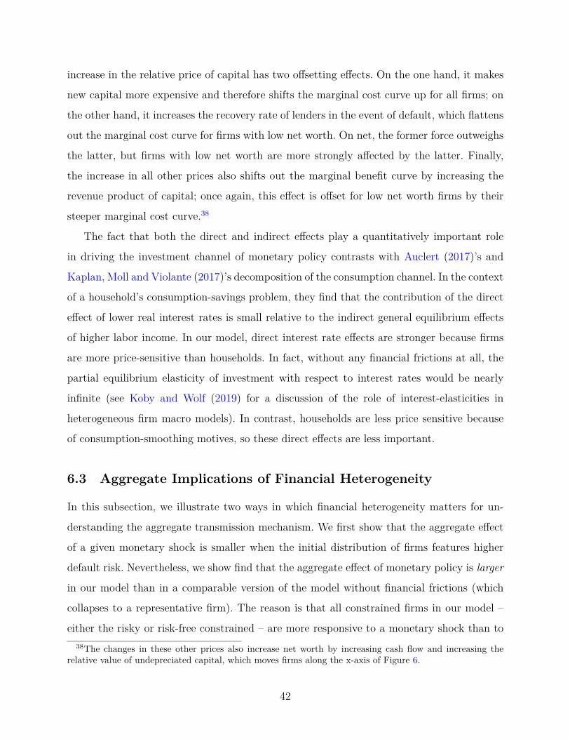
increase in the relative price of capital has two offsetting effects. On the one hand, it makes

new capital more expensive and therefore shifts the marginal cost curve up for all firms; on

the other hand, it increases the recovery rate of lenders in the event of default, which flattens

out the marginal cost curve for firms with low net worth. On net, the former force outweighs

the latter, but firms with low net worth are more strongly affected by the latter. Finally,

the increase in all other prices also shifts out the marginal benefit curve by increasing the

revenue product of capital; once again, this effect is offset for low net worth firms by their

steeper marginal cost curve.38

The fact that both the direct and indirect effects play a quantitatively important role

in driving the investment channel of monetary policy contrasts with Auclert (2017)’s and

Kaplan, Moll and Violante (2017)’s decomposition of the consumption channel. In the context

of a household’s consumption-savings problem, they find that the contribution of the direct

effect of lower real interest rates is small relative to the indirect general equilibrium effects

of higher labor income. In our model, direct interest rate effects are stronger because firms

are more price-sensitive than households. In fact, without any financial frictions at all, the

partial equilibrium elasticity of investment with respect to interest rates would be nearly

infinite (see Koby and Wolf (2019) for a discussion of the role of interest-elasticities in

heterogeneous firm macro models). In contrast, households are less price sensitive because

of consumption-smoothing motives, so these direct effects are less important.

6.3 Aggregate Implications of Financial Heterogeneity

In this subsection, we illustrate two ways in which financial heterogeneity matters for un-

derstanding the aggregate transmission mechanism. We first show that the aggregate effect

of a given monetary shock is smaller when the initial distribution of firms features higher

default risk. Nevertheless, we show find that the aggregate effect of monetary policy is larger

in our model than in a comparable version of the model without financial frictions (which

collapses to a representative firm). The reason is that all constrained firms in our model –

either the risky or risk-free constrained – are more responsive to a monetary shock than to38The changes in these other prices also increase net worth by increasing cash flow and increasing the

relative value of undepreciated capital, which moves firms along the x-axis of Figure 6.

42

a completely unconstrained firm.

State Dependence of Aggregate Transmission In order to illustrate the quantitative

scope for state dependence, we perform a simple back-of-the-envelope calculation: we fix the

semi-elasticity of capital respect to monetary policy as a function of firms’ state variables

and vary the initial distribution of firms.39 We vary the initial distribution of firms µ(z, n)

by taking the weighted average of two reference distributions. The first reference distribution

is the steady-state distribution µ∗(z, n). The second reference distribution µ(z, n) assumes

that the conditional distribution of net worth for every level of productivity is equal to

the distribution of net worth conditional on the lowest realization of productivity in steady

state.40 We then compute the initial distribution as a weighted average of these two reference

distributions, µ(z, n) = ωµ(z, n) + (1 − ω)µ∗(z, n). We vary ω ∈ [0, 1] to trace out linear

combinations of distributions between the steady state (ω = 0) and the low net worth

(ω = 1) distributions.

The left panel of Figure 7 shows that the change in the aggregate capital stock is 60%

smaller starting from the low-net worth distribution µ(z, n) than starting from the steady

state distribution µ∗(z, n). Average net worth is 70% lower and there are 50% more risky

constrained firms in the low-net worth distribution than in the steady state distribution.

The right panel of Figure 7 shows that this effect is due to the fact that the low-net worth

distribution µ(z, n) places more mass in the region of the state space where the elasticity of

capital with respect to the monetary policy shock is low.

These results suggests a potentially powerful source of time-variation in the aggregate

transmission mechanism: monetary policy is less powerful when net worth is low and default39This exercise does not allow for prices to vary with the initial distribution. However, it is a nevertheless an

important necessary condition for the general equilibrium model to generate state dependence. We performthis simple exercise of fixing the elasticities and varying the distribution for two reasons. First, since we donot have to re-compute the equilibrium transition path for each initial distribution, we can investigate statedependence with respect to a large number of initial distributions. Second, it clearly isolates the impact ofvarying the initial distribution from the additional changes to firms’ policy rules arising from changes inprices.

In this exercise, markets do not clear for a given initial distribution of cash-on-hand. We use the elasticitiesfrom the representative firm prices so that markets do not clear for any initial distribution. If we had usedthe equilibrium elasticities, markets would clear for some initial distributions and not others, potentiallybiasing our interpretation of the results.

40We normalize the second reference distribution so that the marginal distribution of productivity is thesame as in the steady state distribution.

43

Figure 7: Aggregate Response Depends on Initial Distribution

0.3 0.4 0.5 0.6 0.7 0.8 0.9 1Average net worth, rel. to S.S.

0.4

0.5

0.6

0.7

0.8

0.9

1

Aggregate

CapitalResponse,Rel.to

S.S.

State Dependence in Aggregate Response

← Low Cash Distribution

Steady State Distribution →

1 2 3 4 5 6 7 8 9 10Net worth

-0.5

0

0.5

1

1.5

2

2.5

3

Sem

i-Elasticity

0

0.05

0.1

0.15

0.2

0.25

0.3

0.35

Mas

s of

firm

s

Capital Semi-Elasticity and Distribution, High Productivity

Steady state distribution

Low net worth distribution

Notes: Dependence of aggregate response on initial distribution. We compute the change in aggregatecapital for different initial distributions using the response to monetary policy computed under the pricepath from the representative firm model. We vary the initial distribution of firms in production µ(z, n) bytaking the weighted average of two reference distributions; see main text for details.

Figure 8: Aggregate Impulse Responses in Full Model vs. Rep Firm Model

2 4 6 8 10Quarters

-0.8

-0.6

-0.4

-0.2

0

Annualizedp.p.deviation

Real Interest Rate

Het agent

Rep agent

2 4 6 8 10Quarters

-0.5

0

0.5

1

1.5

%deviation

Aggregate Investment

Notes: Aggregate impulse responses to a εm0 = −0.0025 innovation to the Taylor rule which decays at rate

ρm = 0.5. Computed as the perfect foresight transition in response to a series of unexpected innovationsstarting from steady state. “Het agent” refers to calibrated heterogeneous firm model from the main text.“Rep agent” refers to a version of the model in which the heterogeneous production sector is replaced by arepresentative firm with the same production function and no financial frictions.

risk is high. Of course, a limitation of this analysis is that we have varied the initial distri-

bution exogenously. The natural next step in this analysis is to incorporate various business

cycle shocks into our model and study the shapes of the distributions that actually arise in

equilibrium.

44

Comparison to Frictionless Model We now compare our full model to a model in

which we eliminate financial frictions. We do so by removing the non-negativity constraint

on dividends; in this case, the investment block of the model collapses to a financially un-

constrained representative firm (see Khan and Thomas (2008) Appendix B). Figure 8 shows

that the impact effect of monetary policy on investment is 25% larger in our full model than

in the representative firm benchmark. Hence, despite the fact that risky constrained firms

are less responsive than risk-free constrained firms, both types of constrained firms are more

responsive than completely unconstrained firms (which, by construction, are the same as

the representative firm in the frictionless benchmark). This occurs because the constrained

firms’ marginal value of net worth is strictly larger than for the unconstrained firms. Their

higher investment demand puts additional upward pressure on the relative price of capital

qt in our full model, which then induces unconstrained firms to disinvest.

7 Conclusion

In this paper, we have argued that financial frictions dampen the response of investment for

firms with high default risk. Our argument had two main components. First, we showed in

the micro data that firms with high leverage or low credit ratings invest significantly less

than other firms following a monetary policy shock. Second, we built a heterogeneous firm

New Keynesian model with default risk that is quantitatively consistent with these empiri-

cal results. In the model, monetary policy stimulates investment through a combination of

direct and indirect effects. High-risk firms are less responsive to these changes because their

marginal cost of investment finance is higher than for low-risk firms. The aggregate effect

of monetary policy is primarily driven by these low-risk firms, which suggests a novel form

of state dependence: monetary policy is less powerful when default risk in the economy is

greater.

Our results may be of independent interest to policymakers who are concerned about

the distributional implications of monetary policy across firms. An often-discussed goal of

monetary policy is to provide resources to viable but credit constrained firms. Many poli-

cymakers’ conventional wisdom, built on the financial accelerator mechanism, suggests that

45

constrained firms will significantly increase their capital investment in response to expan-

sionary monetary policy. Our results imply that, instead, expansionary policy will stimulate

the less risky firms in the economy.

46

ReferencesAndrews, I., M. Gentzkow, and J. Shapiro (2017): “Measuring the sensitivity of parameter

estimates to estimation moments,” The Quarterly Journal of Economics, 132(4), 1553–1592.Arellano, C., Y. Bai, and P. Kehoe (2016): “Financial Frictions and Fluctuations in Volatil-

ity,” Working paper.Arellano, C., L. Maliar, S. Maliar, and V. Tsyrennikov (2016): “Envelope Condition

Methods With an Application to Default Risk Models,” Journal of Economic Dynamics andControl, 69, 436–459.

Asquith, P., and D. W. Mullins (1986): “Equity issues and offering dilution,” Journal offinancial economics, 15, 61–89.

Auclert, A. (2017): “Monetary policy and the redistribution channel,” working paper.Bernanke, B. S., M. Gertler, and S. Gilchrist (1999): “The financial accelerator in a

quantitative business cycle framework,” Handbook of macroeconomics, pp. 1341–1393.Blanco, J. A., and G. Navarro (2016): “The Unemployment Accelerator,” Working paper.Bloom, N., M. Floetotto, N. Jaimovich, I. S. Eksten, and S. Terry (2015): “Really

Uncertain Business Cycles,” Working paper.Buera, F., and S. Karmakar (2017): “Real Effects of Financial Distress: The Role of Hetero-

geneity,” Working paper.Campbell, J., J. Fisher, A. Justiano, and L. Melosi (2016): “Forward Guidance and Macroe-

conomic Outcomes Since the Financial Crisis,” NBER Macroeconomics Annual, 31, 283–357.Christiano, L. J., M. Eichenbaum, and C. L. Evans (2005): “Nominal rigidities and the

dynamic effects of a shock to monetary policy,” Journal of Political Economy, 113, 1–45.Clausen, A., and C. Strub (2017): “A General and Intuitive Envelope Theorem,” Working

paper.Clementi, G. L., and B. Palazzo (2015): “Investment and the Cross-Section of Equity Returns,”

Working paper.Cloyne, J., C. Ferreira, M. Froemel, and P. Surico (2018): “Monetary Policy, Corporate

Finance and Investment,” No. w25366. national bureau of economic research, 2018.Cook, T., and T. Hahn (1989): “The effect of changes in the federal funds rate target on market

interest rates in the 1970s.,” Journal of Monetary Economics, 24, 331–351.Cooley, T. F., and V. Quadrini (2001): “Financial markets and firm dynamics,” American

Economic Review, pp. 1286–1310.Cooper, R. W., and J. C. Haltiwanger (2006): “On the nature of capital adjustment costs,”

The Review of Economic Studies, 73, 611–633.Crouzet, N., and N. Mehrotra (2017): “Small and Large Firms Over the Business Cycle,”

Working paper.Davis, S. J., R. J. Faberman, J. C. Haltiwanger, and I. Rucker (2010): “Adjusted Estimates

of Worker Flows and Job Openings in JOLTS,” Labor in the New Economy, 71, 187.Davis, S. J., J. Haltiwanger, R. Jarmin, and J. Miranda (2006): “Volatility and dispersion

in business growth rates: Publicly traded versus privately held firms,” NBER macroeconomicsannual, 21, 107–179.

DeAngelo, H., L. DeAngelo, and R. M. Stulz (2010): “Seasoned equity offerings, markettiming, and the corporate lifecycle,” Journal of Financial Economics, 95, 275–295.

Dinlersoz, E., S. Kalemli-Ozcan, H. Hyatt, , and V. Penciakova (2018a): “Leverage overthe life cycle and implications for firm growth and shock responsiveness,” No. w25226. nationalbureau of economic research.

47

Dinlersoz, E., S. Kalemli-Ozcan, H. Hyatt, and V. Penciakova (2018b): “Leverage overthe life cycle and implications for firm growth and shock responsiveness,” Discussion paper,National Bureau of Economic Research.

Eberly, J., S. Rebelo, and N. Vincent (2012): “What Explains the Lagged-Investment Dy-namics?,” Journal of Monetary Economics, 59, 370–380.

Eisfeldt, A. L., and A. A. Rampini (2006): “Capital Reallocation and Liquidity,” Journal ofMonetary Economics, 53, 369–399.

Foster, L., J. Haltiwanger, and C. Syverson (2016): “The Slow Growth of New Plants:Learning About Demand?,” Economica, 83, 91–129.

Gavazza, A., S. Mongey, and G. L. Violante (2018): “Aggregate recruiting intensity,” Amer-ican Economic Review, 108(8), 2088–2127.

Gertler, M., and S. Gilchrist (1994): “Monetary Policy, Business Cycles, and the Behavior ofSmall Manufacturing Firms,” The Quarterly Journal of Economics, pp. 309–340.

Gertler, M., and P. Karadi (2015): “Monetary policy surprises, credit costs, and economicactivity,” American Economic Journal: Macroeconomics, 7(1), 44–76.

Gilchrist, S., J. Sim, and E. Zakrajsek (2014): “Uncertainty, Financial Frictions, and Invest-ment Dynamics,” Working paper.

Gilchrist, S., and E. Zakrajšek (2012): “Credit spreads and business cycle fluctuations,”American Economic Review, 102(4), 1692–1720.

Gomes, J. (2001): “Financing Investment,” The American Economic Review, pp. 1263–1285.Gorodnichenko, Y., and M. Weber (2016): “Are sticky prices costly? Evidence from the stock

market,” The American Economic Review, 106, 165–199.Gurkaynak, R. S., B. Sack, and E. T. Swanson (2005): “Do Actions Speak Louder Than

Words? The Response of Asset Prices to Monetary Policy Actions and Statements,” InternationalJournal of Central Banking.

Hennessy, C., and T. Whited (2005): “Debt dynamics,” The Journal of Finance, 60, 1129–1165.Hennessy, C., and T. Whited (2007): “How Costly is External Finance? Evidence from a

Structural Estimation,” The Journal of Finance, 62, 1705.Ippolito, F., A. Ozdagli, and A. Perez-Orive (2017): “The Transmission of Monetary Policy

Through Bank Lending: The Floating Rate Channel,” Working paper.Jeenas, P. (2018): “Firm Balance Sheet Liquidity, Monetary Policy Shocks, and Investment Dy-

namics,” Working paper.Jorda, O. (2005): “Estimation and Inference of Impulse Responses by Local Projections,” The

American Economic Review, 95, 161–182.Kaplan, G., B. Moll, and G. L. Violante (2017): “Monetary policy according to HANK,” .Karabarbounis, L., and B. Neiman (2013): “The Global Decline of the Labor Share,” The

Quarterly Journal of Economics, 129, 61–103.Kashyap, A. K., O. A. Lamont, and J. C. Stein (1994): “Credit Conditions and the Cyclical

Behavior of Inventories,” The Quarterly Journal of Economics, 109, 565–592.Kashyap, A. K., and J. C. Stein (1995): “The impact of monetary policy on bank balance

sheets,” Carnegie-Rochester Conference Series on Public Policy, 42.Khan, A., T. Senga, and J. Thomas (2016): “Default Risk and Aggregate Fluctuations in an

Economy with Production Heterogeneity,” Working paper.Khan, A., and J. Thomas (2008): “Idiosyncratic Shocks and the Role of Nonconvexities in Plant

and Aggregate Investment Dynamics,” Econometrica, 76, 395.(2013): “Credit Shocks and Aggregate Fluctuations in an Economy with Production Het-

48

erogeneity,” Journal of Political Economy, 121, 1055–1107.Koby, Y., and C. Wolf (2019): “Investment Stimulus: From Micro Elasticities to Macro Coun-

terfactuals,” Unpublished manuscript.McKay, A., E. Nakamura, and J. Steinsson (2015): “The power of forward guidance revisited,”

No. w20882. National Bureau of Economic Research.McKay, A., and J. F. Wieland (2019): “Lumpy Durable Consumption Demand and the Limited

Ammunition of Monetary Policy,” .Merton, R. C. (1974): “On the pricing of corporate debt: The risk structure of interest rates,”

The Journal of Finance, 29, 449–470.Miranda-Agrippino, S., and G. Ricco (2018): “The transmission of monetary policy shocks,”

Working paper.Nakamura, E., and J. Steinsson (2013): “High frequency identification of monetary non-

neutrality,” No. w19260. National Bureau of Economic Research.Romer, C., and D. Romer (1990): “New Evidence on the Monetary Transmission Mechanism,”

Brookings Papers on Economic Activity, 21, 149–214.Schaefer, S. M., and I. A. Strebulaev (2008): “Structural models of credit risk are useful:

Evidence from hedge ratios on corporate bonds,” Journal of Financial Economics, 90(1), 1–19.Smith, C. W. (1977): “Alternative methods for raising capital: Rights versus underwritten offer-

ings,” Journal of financial economics, 5, 273–307.Tenreyro, S., and G. Thwaites (2016): “Pushing on a string: US monetary policy is less

powerful in recessions,” American Economic Journal: Macroeconomics, 8(4), 43–74.Vavra, J. (2013): “Inflation dynamics and time-varying volatility: New evidence and an ss inter-

pretation,” The Quarterly Journal of Economics, 129(1), 215–258.Whited, T. M. (1992): “Debt, Liquidity Constraints, and Corporate Investment: Evidence from

Panel Data,” The Journal of Finance, 47, 1425–1460.Wilmer, Cutler, Pickering, Hale, and D. LLP (2017): “2017 IPO Report,” Technical report.Wong, A. (2016): “Transmission of Monetary Policy to Consumption and Population Aging,”

working paper.Zwick, E., and J. Mahon (2017): “Tax policy and heterogeneous investment behavior,” American

Economic Review, 107(1), 217–48.

49

Appendix (For Online Publication Only)

A Empirical Appendix

This appendix contains additional results related to the empirical work in Section 2. Ap-

pendix A.1 describes the construction and cleaning of our dataset. Appendix A.2 shows that

our main empirical results are robust along a number of dimensions. Appendix A.3 contains

additional empirical results referenced in the main text. Finally, Appendix A.4 compares our

results to others in the literature, such as Gertler and Gilchrist (1994), Cloyne et al. (2018),

and Jeenas (2018).

A.1 Data Construction

This subsection describes the firm-level variables used in the empirical analysis of the paper,

based on quarterly Compustat data. The definition of the variables and sample selection

follow standard practices in the literature (see, for example, Whited, 1992; Gomes, 2001;

Eisfeldt and Rampini, 2006; Clementi and Palazzo, 2015).

Variables

1. Investment, intensive margin (baseline measure): defined as ∆ log(kjt+1), where kjt+1

denotes the capital stock of firm j at the end of period t. For each firm, we set the first

value of kjt+1 to the level of gross plant, property, and equipment (ppegtq, item 118) in

the first period in which this variable is reported in Compustat. From this period onwards,

we compute the evolution of kjt+1 using the changes of net plant, property, and equipment

(ppentq, item 42), which is a measure net investment with significantly more observations

than ppegtq (net of depreciation). If a firm has a missing observation of ppentq located

between two periods with nonmissing observations we estimate its value using a linear

interpolation with the values of ppentq right before and after the missing observation; if

two or more consecutive observations are missing we do not do any imputation. We only

consider investment spells with 40 quarters or more in order to precisely estimate fixed

effects.

50

2. Leverage: defined as the ratio of total debt (sum of dlcq and dlttq, items 45 and 71) to

total assets (atq, item 44).

3. Net leverage: defined as the ratio of total debt minus net current assets (actq, item 40,

minus lctq, item 49) to total assets.

4. Distance to default: Following Merton (1974) and Gilchrist and Zakrajšek (2012), we define

this variable as dd ≡ log(V/D)+(µV −0.5σ2V )

σV, where V denotes the total value of the firm, µV

the expected return on V , σV the volatility of the firm’s value, and D firm’s debt.41 To

estimate the firm’s value V , we follow an iterative procedure, based on Gilchrist and

Zakrajšek (2012) and Blanco and Navarro (2016):

i. Set an initial value for the firm value equal to the sum of firm debt and equity,

V = E+D, where E is measured as the firm’s stock price times the number of shares

(data source: CRSP).

ii. Estimate the mean and variance of return on firm value over a 250-day moving win-

dow. The return on firm value is measured as the daily log return on assets, ∆ log V .

iii. Obtain a new estimate of V for every day of the 250-day moving window from the

Black-Scholes-Merton option-pricing framework E = V Φ(δ1) − e−rTDΦ(δ2), where

δ1 ≡log(V/D)+(r+0.5σ2

V )T

σ2V

√T

, and δ2 ≡ δ1 − σV

√T , where r is the daily one-year constant

maturity Treasury-yield (data source: Federal Reserve Board of Governors H.15 Se-

lected Interest Rates release).

iv. Iterate on steps [ii.] and [iii.] until convergence.

5. Real sales growth: measured as log-differences in sales (saleq, item 2) deflated using CPI.

6. Size: measured as the log of total assets.

7. Liquidity: defined as the ratio of cash and short-term investments (cheq, item 36) to total

assets.41We measure the face value of debt D as the sum of the firm’s short-term debt (dlcq, item 45) and one-

half of long-term debt (dlttq, item 71), following Gilchrist and Zakrajšek (2012) and a common practice bycredit rating agencies (Moody’s/KMV).

51

8. Cash flow: measured as EBITDA divided by capital stock.

9. Dividend payer: defined as a dummy variable taking a value of one in firm-quarter obser-

vations in which the firm paid dividends to preferred stock of the company (constructed

using dvpq, item 24).

10. Tobin’s q: defined as the ratio market to book value of assets. The market value of assets

is measured as the book value, plus the market value of common stock, minus the book

value of common stock ceq, plus deferred taxes and investment tax credit (item txditcq,

item 52). The market value of common stock is computed as the product of price at

quarter close (prccq) and common shares outstanding (cshoq item 61). We winsorize 1%

of observations in each tail of the distribution.

11. Sectoral dummies. We consider the following sectors: (i) agriculture, forestry, and fishing:

sic < 10; (ii) mining: sic∈ [10, 14]; (iii) construction: sic∈ [15, 17]; (iv) manufacturing:

sic∈ [20, 39]; (v) transportation, communications, electric, gas, and sanitary services:

sic∈ [40, 49]; (vi) wholesale trade: sic∈ [50, 51]; (vii) retail trade sic∈ [52, 59]; (viii)

services: sic∈ [70, 89].

Sample Selection Our empirical analysis excludes (in order of operation):

1. Firms in finance, insurance, and real estate sectors (sic∈ [60, 67]) and public administra-

tion (sic∈ [91, 97]).

2. Firms not incorporated in the United States.

3. Firm-quarter observations with acquisitions (constructed based on aqcy, item 94) larger

than 5% percent of assets.

4. Firm-quarter observations that satisfy one of the following conditions, aimed at excluding

extreme observations:

i. Investment rate is in the top and bottom 0.5 percent of the distribution.

ii. Leverage higher than 10.

52

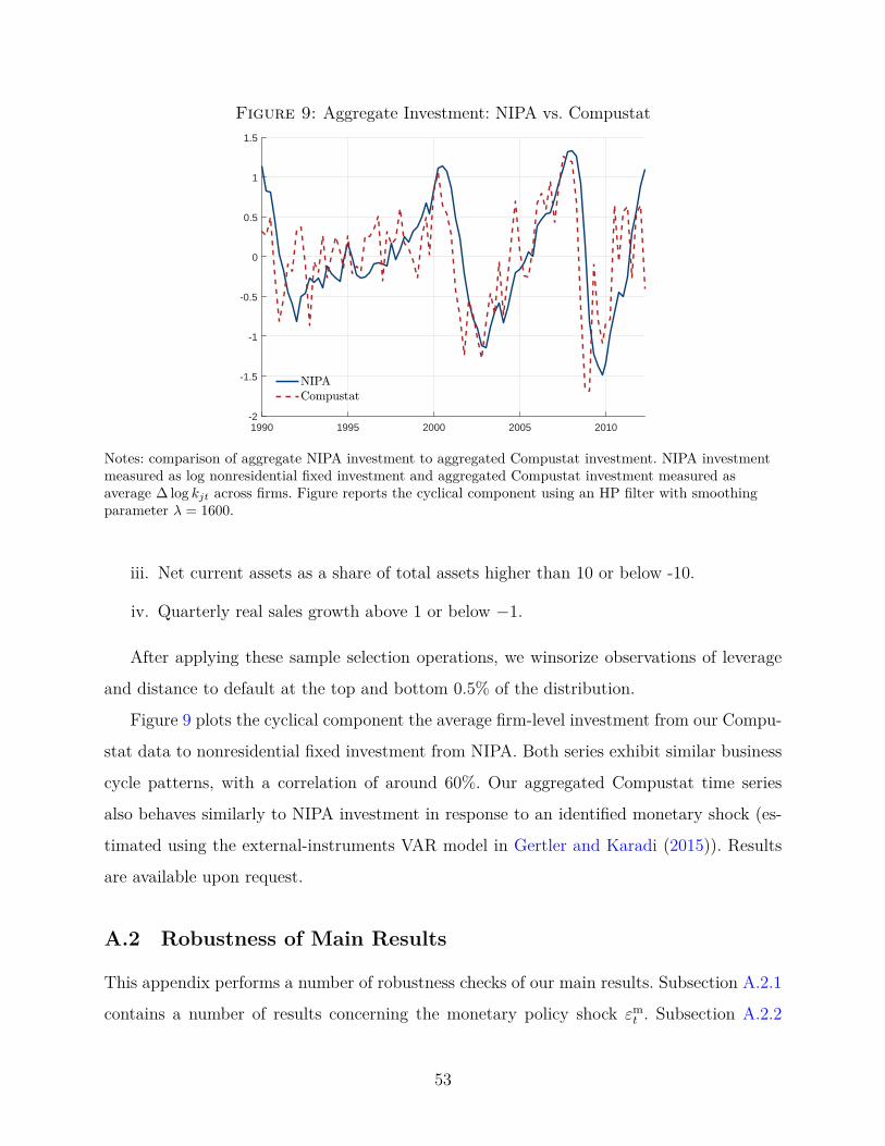
Figure 9: Aggregate Investment: NIPA vs. Compustat

1990 1995 2000 2005 2010-2

-1.5

-1

-0.5

0

0.5

1

1.5

Notes: comparison of aggregate NIPA investment to aggregated Compustat investment. NIPA investmentmeasured as log nonresidential fixed investment and aggregated Compustat investment measured asaverage ∆log kjt across firms. Figure reports the cyclical component using an HP filter with smoothingparameter λ = 1600.

iii. Net current assets as a share of total assets higher than 10 or below -10.

iv. Quarterly real sales growth above 1 or below −1.

After applying these sample selection operations, we winsorize observations of leverage

and distance to default at the top and bottom 0.5% of the distribution.

Figure 9 plots the cyclical component the average firm-level investment from our Compu-

stat data to nonresidential fixed investment from NIPA. Both series exhibit similar business

cycle patterns, with a correlation of around 60%. Our aggregated Compustat time series

also behaves similarly to NIPA investment in response to an identified monetary shock (es-

timated using the external-instruments VAR model in Gertler and Karadi (2015)). Results

are available upon request.

A.2 Robustness of Main Results

This appendix performs a number of robustness checks of our main results. Subsection A.2.1

contains a number of results concerning the monetary policy shock εmt . Subsection A.2.2

53

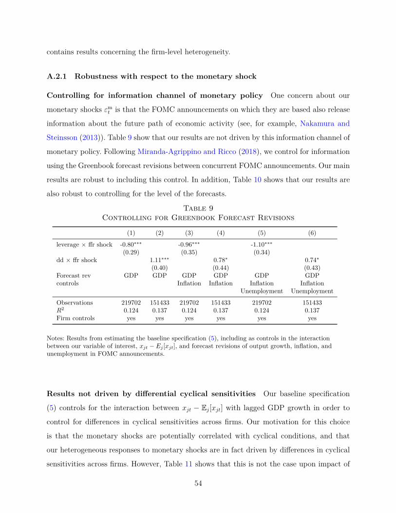
contains results concerning the firm-level heterogeneity.

A.2.1 Robustness with respect to the monetary shock

Controlling for information channel of monetary policy One concern about our

monetary shocks εmt is that the FOMC announcements on which they are based also release

information about the future path of economic activity (see, for example, Nakamura and

Steinsson (2013)). Table 9 show that our results are not driven by this information channel of

monetary policy. Following Miranda-Agrippino and Ricco (2018), we control for information

using the Greenbook forecast revisions between concurrent FOMC announcements. Our main

results are robust to including this control. In addition, Table 10 shows that our results are

also robust to controlling for the level of the forecasts.

Table 9Controlling for Greenbook Forecast Revisions

(1) (2) (3) (4) (5) (6)

leverage × ffr shock -0.80∗∗∗ -0.96∗∗∗ -1.10∗∗∗(0.29) (0.35) (0.34)

dd × ffr shock 1.11∗∗∗ 0.78∗ 0.74∗(0.40) (0.44) (0.43)

Forecast rev GDP GDP GDP GDP GDP GDPcontrols Inflation Inflation Inflation Inflation

Unemployment Unemployment

Observations 219702 151433 219702 151433 219702 151433R2 0.124 0.137 0.124 0.137 0.124 0.137Firm controls yes yes yes yes yes yes

Notes: Results from estimating the baseline specification (5), including as controls in the interactionbetween our variable of interest, xjt − Ej [xjt], and forecast revisions of output growth, inflation, andunemployment in FOMC announcements.

Results not driven by differential cyclical sensitivities Our baseline specification

(5) controls for the interaction between xjt − Ej[xjt] with lagged GDP growth in order to

control for differences in cyclical sensitivities across firms. Our motivation for this choice

is that the monetary shocks are potentially correlated with cyclical conditions, and that

our heterogeneous responses to monetary shocks are in fact driven by differences in cyclical

sensitivities across firms. However, Table 11 shows that this is not the case upon impact of

54

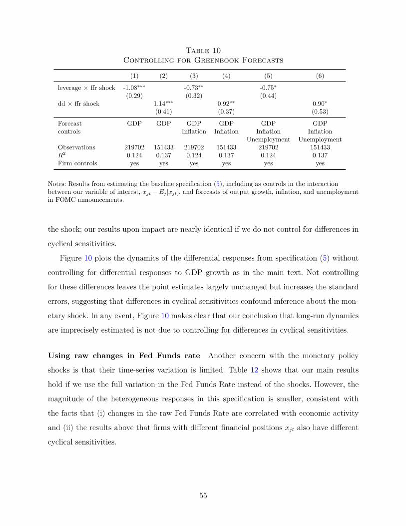
Table 10Controlling for Greenbook Forecasts

(1) (2) (3) (4) (5) (6)

leverage × ffr shock -1.08∗∗∗ -0.73∗∗ -0.75∗(0.29) (0.32) (0.44)

dd × ffr shock 1.14∗∗∗ 0.92∗∗ 0.90∗(0.41) (0.37) (0.53)

Forecast GDP GDP GDP GDP GDP GDPcontrols Inflation Inflation Inflation Inflation

Unemployment UnemploymentObservations 219702 151433 219702 151433 219702 151433R2 0.124 0.137 0.124 0.137 0.124 0.137Firm controls yes yes yes yes yes yes

Notes: Results from estimating the baseline specification (5), including as controls in the interactionbetween our variable of interest, xjt −Ej [xjt], and forecasts of output growth, inflation, and unemploymentin FOMC announcements.

the shock; our results upon impact are nearly identical if we do not control for differences in

cyclical sensitivities.

Figure 10 plots the dynamics of the differential responses from specification (5) without

controlling for differential responses to GDP growth as in the main text. Not controlling

for these differences leaves the point estimates largely unchanged but increases the standard

errors, suggesting that differences in cyclical sensitivities confound inference about the mon-

etary shock. In any event, Figure 10 makes clear that our conclusion that long-run dynamics

are imprecisely estimated is not due to controlling for differences in cyclical sensitivities.

Using raw changes in Fed Funds rate Another concern with the monetary policy

shocks is that their time-series variation is limited. Table 12 shows that our main results

hold if we use the full variation in the Fed Funds Rate instead of the shocks. However, the

magnitude of the heterogeneous responses in this specification is smaller, consistent with

the facts that (i) changes in the raw Fed Funds Rate are correlated with economic activity

and (ii) the results above that firms with different financial positions xjt also have different

cyclical sensitivities.

55

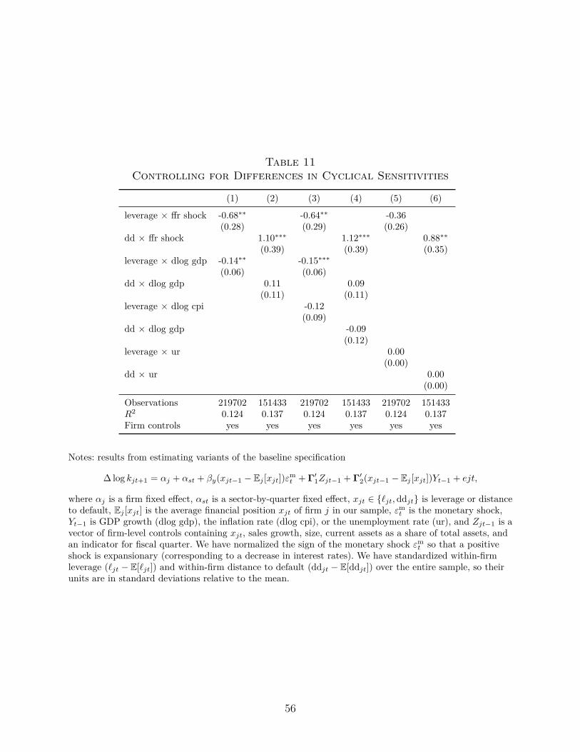
Table 11Controlling for Differences in Cyclical Sensitivities

(1) (2) (3) (4) (5) (6)

leverage × ffr shock -0.68∗∗ -0.64∗∗ -0.36(0.28) (0.29) (0.26)

dd × ffr shock 1.10∗∗∗ 1.12∗∗∗ 0.88∗∗(0.39) (0.39) (0.35)

leverage × dlog gdp -0.14∗∗ -0.15∗∗∗(0.06) (0.06)

dd × dlog gdp 0.11 0.09(0.11) (0.11)

leverage × dlog cpi -0.12(0.09)

dd × dlog gdp -0.09(0.12)

leverage × ur 0.00(0.00)

dd × ur 0.00(0.00)

Observations 219702 151433 219702 151433 219702 151433R2 0.124 0.137 0.124 0.137 0.124 0.137Firm controls yes yes yes yes yes yes

Notes: results from estimating variants of the baseline specification

∆log kjt+1 = αj + αst + βy(xjt−1 − Ej [xjt])εmt + Γ′

1Zjt−1 + Γ′2(xjt−1 − Ej [xjt])Yt−1 + ejt,

where αj is a firm fixed effect, αst is a sector-by-quarter fixed effect, xjt ∈ {ℓjt,ddjt} is leverage or distanceto default, Ej [xjt] is the average financial position xjt of firm j in our sample, εm

t is the monetary shock,Yt−1 is GDP growth (dlog gdp), the inflation rate (dlog cpi), or the unemployment rate (ur), and Zjt−1 is avector of firm-level controls containing xjt, sales growth, size, current assets as a share of total assets, andan indicator for fiscal quarter. We have normalized the sign of the monetary shock εm

t so that a positiveshock is expansionary (corresponding to a decrease in interest rates). We have standardized within-firmleverage (ℓjt − E[ℓjt]) and within-firm distance to default (ddjt − E[ddjt]) over the entire sample, so theirunits are in standard deviations relative to the mean.

56

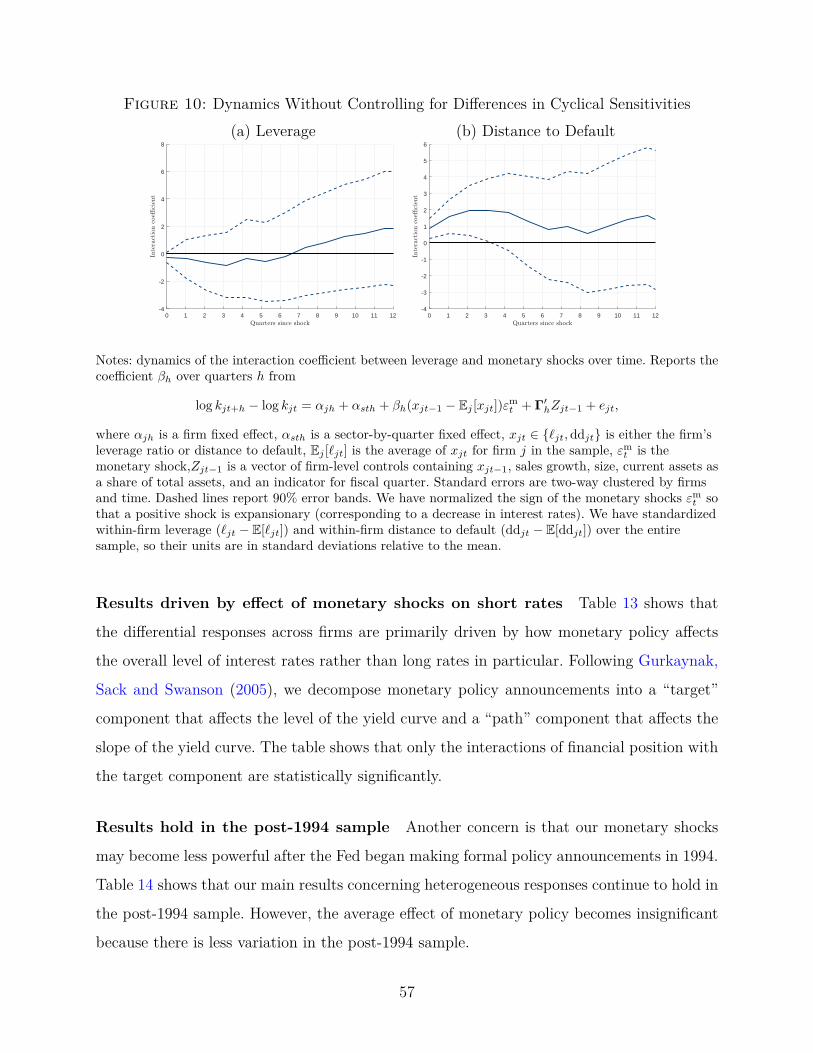
Figure 10: Dynamics Without Controlling for Differences in Cyclical Sensitivities(a) Leverage (b) Distance to Default

0 1 2 3 4 5 6 7 8 9 10 11 12-4

-2

0

2

4

6

8

0 1 2 3 4 5 6 7 8 9 10 11 12-4

-3

-2

-1

0

1

2

3

4

5

6

Notes: dynamics of the interaction coefficient between leverage and monetary shocks over time. Reports thecoefficient βh over quarters h from

log kjt+h − log kjt = αjh + αsth + βh(xjt−1 − Ej [xjt])εmt + Γ′

hZjt−1 + ejt,

where αjh is a firm fixed effect, αsth is a sector-by-quarter fixed effect, xjt ∈ {ℓjt,ddjt} is either the firm’sleverage ratio or distance to default, Ej [ℓjt] is the average of xjt for firm j in the sample, εm

t is themonetary shock,Zjt−1 is a vector of firm-level controls containing xjt−1, sales growth, size, current assets asa share of total assets, and an indicator for fiscal quarter. Standard errors are two-way clustered by firmsand time. Dashed lines report 90% error bands. We have normalized the sign of the monetary shocks εm

t sothat a positive shock is expansionary (corresponding to a decrease in interest rates). We have standardizedwithin-firm leverage (ℓjt − E[ℓjt]) and within-firm distance to default (ddjt − E[ddjt]) over the entiresample, so their units are in standard deviations relative to the mean.

Results driven by effect of monetary shocks on short rates Table 13 shows that

the differential responses across firms are primarily driven by how monetary policy affects

the overall level of interest rates rather than long rates in particular. Following Gurkaynak,

Sack and Swanson (2005), we decompose monetary policy announcements into a “target”

component that affects the level of the yield curve and a “path” component that affects the

slope of the yield curve. The table shows that only the interactions of financial position with

the target component are statistically significantly.

Results hold in the post-1994 sample Another concern is that our monetary shocks

may become less powerful after the Fed began making formal policy announcements in 1994.

Table 14 shows that our main results concerning heterogeneous responses continue to hold in

the post-1994 sample. However, the average effect of monetary policy becomes insignificant

because there is less variation in the post-1994 sample.

57

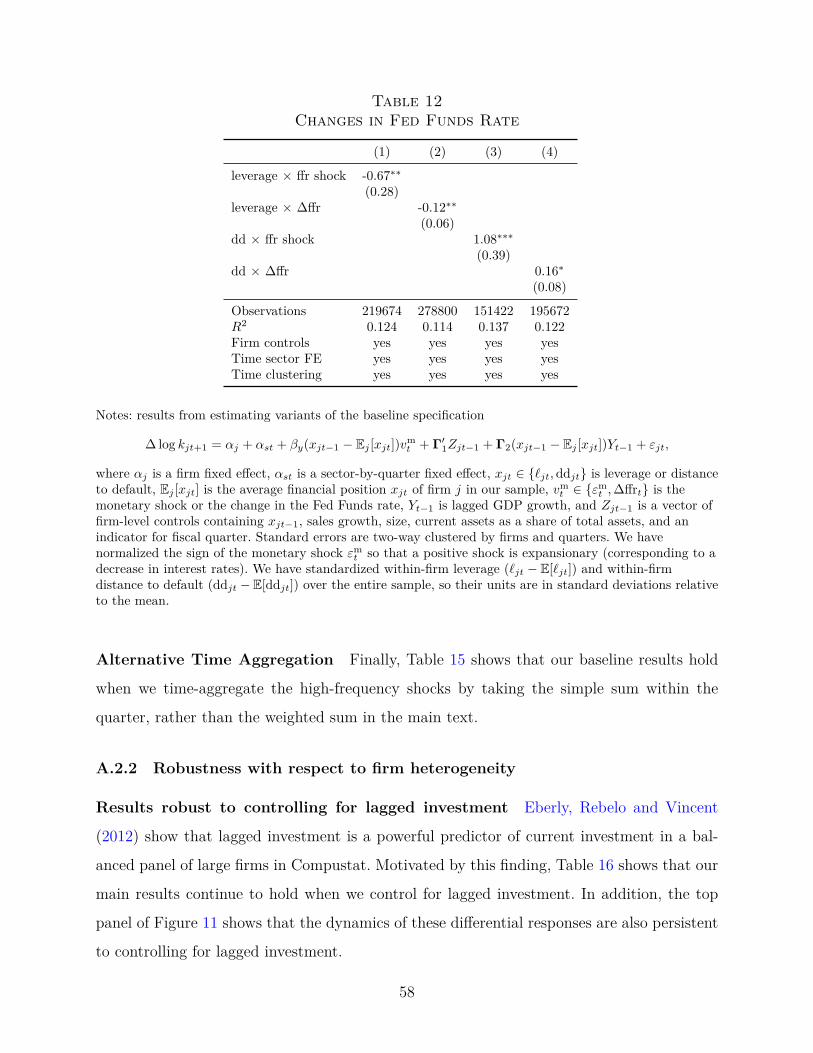
Table 12Changes in Fed Funds Rate

(1) (2) (3) (4)

leverage × ffr shock -0.67∗∗(0.28)

leverage × ∆ffr -0.12∗∗(0.06)

dd × ffr shock 1.08∗∗∗(0.39)

dd × ∆ffr 0.16∗(0.08)

Observations 219674 278800 151422 195672R2 0.124 0.114 0.137 0.122Firm controls yes yes yes yesTime sector FE yes yes yes yesTime clustering yes yes yes yes

Notes: results from estimating variants of the baseline specification

∆log kjt+1 = αj + αst + βy(xjt−1 − Ej [xjt])vmt + Γ′

1Zjt−1 + Γ2(xjt−1 − Ej [xjt])Yt−1 + εjt,

where αj is a firm fixed effect, αst is a sector-by-quarter fixed effect, xjt ∈ {ℓjt,ddjt} is leverage or distanceto default, Ej [xjt] is the average financial position xjt of firm j in our sample, vm

t ∈ {εmt ,∆ffrt} is the

monetary shock or the change in the Fed Funds rate, Yt−1 is lagged GDP growth, and Zjt−1 is a vector offirm-level controls containing xjt−1, sales growth, size, current assets as a share of total assets, and anindicator for fiscal quarter. Standard errors are two-way clustered by firms and quarters. We havenormalized the sign of the monetary shock εm

t so that a positive shock is expansionary (corresponding to adecrease in interest rates). We have standardized within-firm leverage (ℓjt − E[ℓjt]) and within-firmdistance to default (ddjt − E[ddjt]) over the entire sample, so their units are in standard deviations relativeto the mean.

Alternative Time Aggregation Finally, Table 15 shows that our baseline results hold

when we time-aggregate the high-frequency shocks by taking the simple sum within the

quarter, rather than the weighted sum in the main text.

A.2.2 Robustness with respect to firm heterogeneity

Results robust to controlling for lagged investment Eberly, Rebelo and Vincent

(2012) show that lagged investment is a powerful predictor of current investment in a bal-

anced panel of large firms in Compustat. Motivated by this finding, Table 16 shows that our

main results continue to hold when we control for lagged investment. In addition, the top

panel of Figure 11 shows that the dynamics of these differential responses are also persistent

to controlling for lagged investment.

58

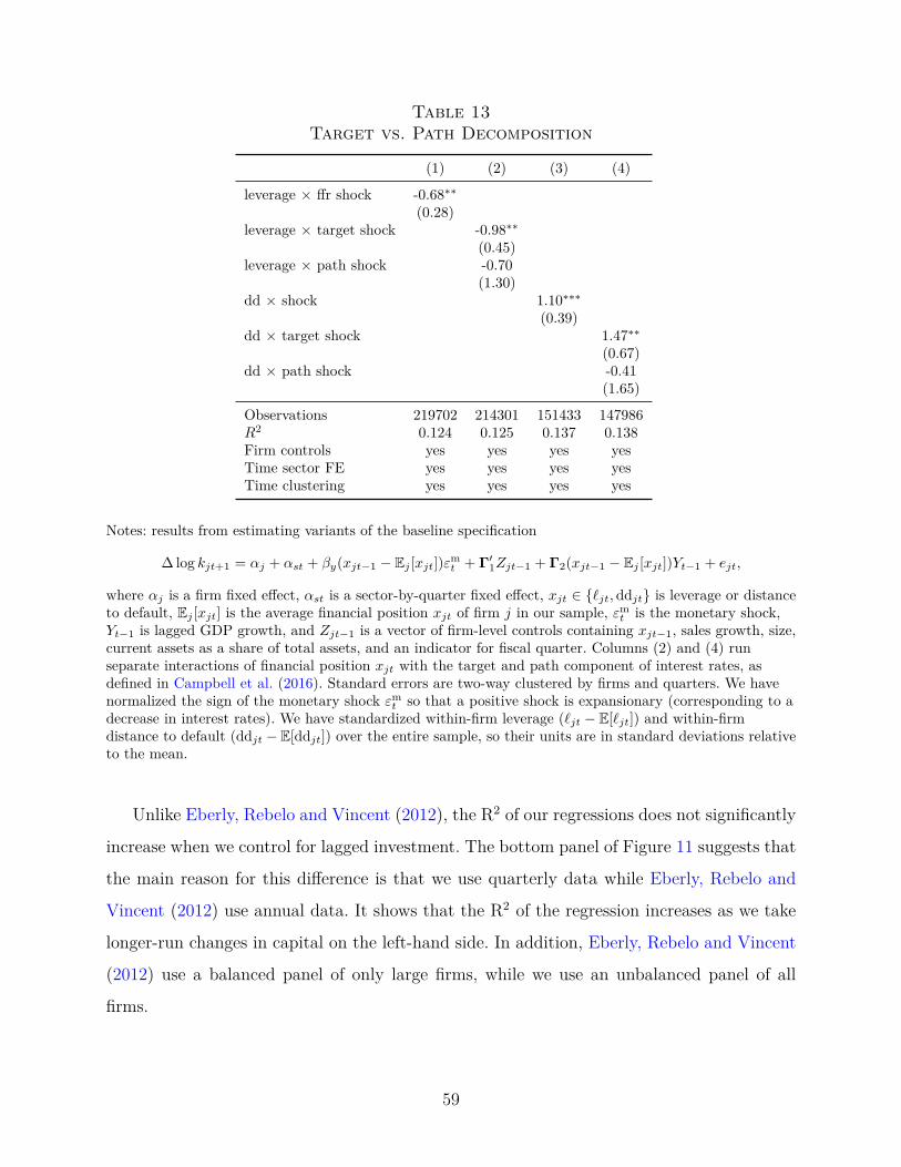
Table 13Target vs. Path Decomposition

(1) (2) (3) (4)

leverage × ffr shock -0.68∗∗(0.28)

leverage × target shock -0.98∗∗(0.45)

leverage × path shock -0.70(1.30)

dd × shock 1.10∗∗∗(0.39)

dd × target shock 1.47∗∗(0.67)

dd × path shock -0.41(1.65)

Observations 219702 214301 151433 147986R2 0.124 0.125 0.137 0.138Firm controls yes yes yes yesTime sector FE yes yes yes yesTime clustering yes yes yes yes

Notes: results from estimating variants of the baseline specification

∆log kjt+1 = αj + αst + βy(xjt−1 − Ej [xjt])εmt + Γ′

1Zjt−1 + Γ2(xjt−1 − Ej [xjt])Yt−1 + ejt,

where αj is a firm fixed effect, αst is a sector-by-quarter fixed effect, xjt ∈ {ℓjt,ddjt} is leverage or distanceto default, Ej [xjt] is the average financial position xjt of firm j in our sample, εm

t is the monetary shock,Yt−1 is lagged GDP growth, and Zjt−1 is a vector of firm-level controls containing xjt−1, sales growth, size,current assets as a share of total assets, and an indicator for fiscal quarter. Columns (2) and (4) runseparate interactions of financial position xjt with the target and path component of interest rates, asdefined in Campbell et al. (2016). Standard errors are two-way clustered by firms and quarters. We havenormalized the sign of the monetary shock εm

t so that a positive shock is expansionary (corresponding to adecrease in interest rates). We have standardized within-firm leverage (ℓjt − E[ℓjt]) and within-firmdistance to default (ddjt − E[ddjt]) over the entire sample, so their units are in standard deviations relativeto the mean.

Unlike Eberly, Rebelo and Vincent (2012), the R2 of our regressions does not significantly

increase when we control for lagged investment. The bottom panel of Figure 11 suggests that

the main reason for this difference is that we use quarterly data while Eberly, Rebelo and

Vincent (2012) use annual data. It shows that the R2 of the regression increases as we take

longer-run changes in capital on the left-hand side. In addition, Eberly, Rebelo and Vincent

(2012) use a balanced panel of only large firms, while we use an unbalanced panel of all

firms.

59

Figure 11: Dynamics Controlling by Lagged Investment(a) Leverage (b) Distance to Default

Interaction coefficient

0 1 2 3 4 5 6 7 8 9 10 11 12-6

-4

-2

0

2

4

6

0 1 2 3 4 5 6 7 8 9 10 11 12-2

0

2

4

6

8

10

R2 of the regression

0 1 2 3 4 5 6 7 8 9 10 11 120.15

0.2

0.25

0.3

0.35

0.4

0.45

0 1 2 3 4 5 6 7 8 9 10 11 120.15

0.2

0.25

0.3

0.35

0.4

0.45

0.5

Notes: dynamics of the interaction coefficient between leverage and monetary shocks over time. Reports thecoefficient βh over quarters h from

log kjt+h− log kjt = αjh+αsth+ρ∆log kjt+βh(xjt−1−Ej [xjt])εmt +Γ′

hZjt−1+Γ′2h(xjt−1−Ej [xjt])Yt−1+ejt,

where αjh is a firm fixed effect, αsth is a sector-by-quarter fixed effect, xjt ∈ {ℓjt,ddjt} is either the firm’sleverage ratio or distance to default, Ej [xjt] is the average of xjt for firm j in the sample, εm

t is themonetary shock,Zjt−1 is a vector of firm-level controls containing xjt−1, sales growth, size, current assets asa share of total assets, and an indicator for fiscal quarter, and Yt−1 is GDP growth. Standard errors aretwo-way clustered by firms and time. Dashed lines report 90% error bands. We have normalized the sign ofthe monetary shocks εm

t so that a positive shock is expansionary (corresponding to a decrease in interestrates). We have standardized within-firm leverage (ℓjt − E[ℓjt]) and within-firm distance to default(ddjt − E[ddjt]) over the entire sample, so their units are in standard deviations relative to the mean.

60

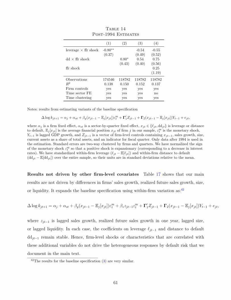
Table 14Post-1994 Estimates

(1) (2) (3) (4)

leverage × ffr shock -0.80∗∗ -0.54 -0.55(0.37) (0.49) (0.52)

dd × ffr shock 0.80∗ 0.54 0.75(0.43) (0.40) (0.56)

ffr shock 0.25(1.19)

Observations 174546 118782 118782 118782R2 0.138 0.150 0.152 0.137Firm controls yes yes yes yesTime sector FE yes yes yes noTime clustering yes yes yes yes

Notes: results from estimating variants of the baseline specification

∆log kjt+1 = αj + αst + βy(xjt−1 − Ej [xjt])εmt + Γ′

1Zjt−1 + Γ2(xjt−1 − Ej [xjt])Yt−1 + ejt,

where αj is a firm fixed effect, αst is a sector-by-quarter fixed effect, xjt ∈ {ℓjt,ddjt} is leverage or distanceto default, Ej [xjt] is the average financial position xjt of firm j in our sample, εm

t is the monetary shock,Yt−1 is lagged GDP growth, and Zjt−1 is a vector of firm-level controls containing xjt−1, sales growth, size,current assets as a share of total assets, and an indicator for fiscal quarter. Only data after 1994 is used inthe estimation. Standard errors are two-way clustered by firms and quarters. We have normalized the signof the monetary shock εm

t so that a positive shock is expansionary (corresponding to a decrease in interestrates). We have standardized within-firm leverage (ℓjt − E[ℓjt]) and within-firm distance to default(ddjt − E[ddjt]) over the entire sample, so their units are in standard deviations relative to the mean.

Results not driven by other firm-level covariates Table 17 shows that our main

results are not driven by differences in firms’ sales growth, realized future sales growth, size,

or liquidity. It expands the baseline specification using within-firm variation as:42

∆ log kjt+1 = αj + αst + βy(xjt−1 − Ej[xjt])εmt + βzzjt−1ε

mt + Γ′

1Zjt−1 + Γ2(xjt−1 − Ej[xjt])Yt−1 + ejt,

where zjt−1 is lagged sales growth, realized future sales growth in one year, lagged size,

or lagged liquidity. In each case, the coefficients on leverage ℓjt−1 and distance to default

ddjt−1 remain stable. Hence, firm-level shocks or characteristics that are correlated with

these additional variables do not drive the heterogeneous responses by default risk that we

document in the main text.42The results for the baseline specification (3) are very similar.

61

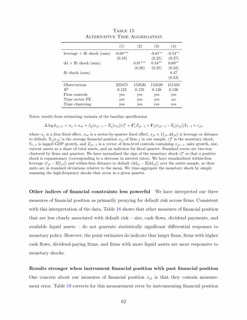
Table 15Alternative Time Aggregation

(1) (2) (3) (4)

leverage × ffr shock (sum) -0.68∗∗∗ -0.61∗∗ -0.54∗∗(0.19) (0.25) (0.27)

dd × ffr shock (sum) 0.81∗∗∗ 0.54∗∗ 0.69∗∗(0.26) (0.25) (0.32)

ffr shock (sum) 0.47(0.53)

Observations 222475 153520 153520 151433R2 0.123 0.135 0.138 0.126Firm controls yes yes yes yesTime sector FE yes yes yes noTime clustering yes yes yes yes

Notes: results from estimating variants of the baseline specification

∆log kjt+1 = αj + αst + βy(xjt−1 − Ej [xjt])εmt + Γ′

1Zjt−1 + Γ2(xjt−1 − Ej [xjt])Yt−1 + εjt,

where αj is a firm fixed effect, αst is a sector-by-quarter fixed effect, xjt ∈ {ℓjt,ddjt} is leverage or distanceto default, Ej [xjt] is the average financial position xjt of firm j in our sample, εm

t is the monetary shock,Yt−1 is lagged GDP growth, and Zjt−1 is a vector of firm-level controls containing xjt−1, sales growth, size,current assets as a share of total assets, and an indicator for fiscal quarter. Standard errors are two-wayclustered by firms and quarters. We have normalized the sign of the monetary shock εm

t so that a positiveshock is expansionary (corresponding to a decrease in interest rates). We have standardized within-firmleverage (ℓjt − E[ℓjt]) and within-firm distance to default (ddjt − E[ddjt]) over the entire sample, so theirunits are in standard deviations relative to the mean. We time-aggregate the monetary shock by simplysumming the high-frequency shocks that occur in a given quarter.

Other indices of financial constraints less powerful We have interpreted our three

measures of financial position as primarily proxying for default risk across firms. Consistent

with this interpretation of the data, Table 18 shows that other measures of financial position

that are less closely associated with default risk – size, cash flows, dividend payments, and

available liquid assets – do not generate statistically significant differential responses to

monetary policy. However, the point estimates do indicate that larger firms, firms with higher

cash flows, dividend-paying firms, and firms with more liquid assets are more responsive to

monetary shocks.

Results stronger when instrument financial position with past financial position

One concern about our measures of financial position xjt is that they contain measure-

ment error. Table 19 corrects for this measurement error by instrumenting financial position

62

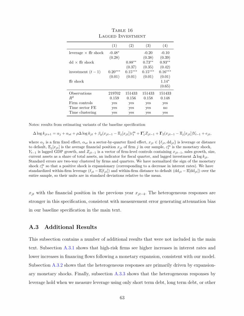
Table 16Lagged Investment

(1) (2) (3) (4)

leverage × ffr shock -0.48∗ -0.20 -0.10(0.28) (0.38) (0.39)

dd × ffr shock 0.88∗∗ 0.73∗∗ 0.93∗∗(0.37) (0.35) (0.42)

investment (t− 1) 0.20∗∗∗ 0.15∗∗∗ 0.15∗∗∗ 0.16∗∗∗(0.01) (0.01) (0.01) (0.01)

ffr shock 1.14∗(0.65)

Observations 219702 151433 151433 151433R2 0.159 0.156 0.158 0.148Firm controls yes yes yes yesTime sector FE yes yes yes noTime clustering yes yes yes yes

Notes: results from estimating variants of the baseline specification

∆log kjt+1 = αj + αst + ρ∆log kjt + βy(xjt−1 − Ej [xjt])εmt + Γ′

1Zjt−1 + Γ2(xjt−1 − Ej [xjt])Yt−1 + ejt,

where αj is a firm fixed effect, αst is a sector-by-quarter fixed effect, xjt ∈ {ℓjt,ddjt} is leverage or distanceto default, Ej [xjt] is the average financial position xjt of firm j in our sample, εm

t is the monetary shock,Yt−1 is lagged GDP growth, and Zjt−1 is a vector of firm-level controls containing xjt−1, sales growth, size,current assets as a share of total assets, an indicator for fiscal quarter, and lagged investment ∆log kjt.Standard errors are two-way clustered by firms and quarters. We have normalized the sign of the monetaryshock εm

t so that a positive shock is expansionary (corresponding to a decrease in interest rates). We havestandardized within-firm leverage (ℓjt −E[ℓjt]) and within-firm distance to default (ddjt −E[ddjt]) over theentire sample, so their units are in standard deviations relative to the mean.

xjt with the financial position in the previous year xjt−4. The heterogeneous responses are

stronger in this specification, consistent with measurement error generating attenuation bias

in our baseline specification in the main text.

A.3 Additional Results

This subsection contains a number of additional results that were not included in the main

text. Subsection A.3.1 shows that high-risk firms see higher increases in interest rates and

lower increases in financing flows following a monetary expansion, consistent with our model.

Subsection A.3.2 shows that the heterogeneous responses are primarily driven by expansion-

ary monetary shocks. Finally, subsection A.3.3 shows that the heterogeneous responses by

leverage hold when we measure leverage using only short term debt, long term debt, or other

63

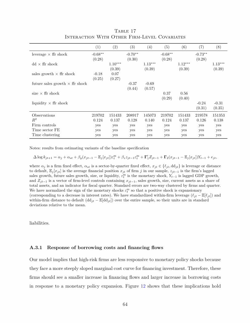
Table 17Interaction With Other Firm-Level Covariates

(1) (2) (3) (4) (5) (6) (7) (8)

leverage × ffr shock -0.68∗∗ -0.70∗∗ -0.68∗∗ -0.73∗∗(0.28) (0.30) (0.28) (0.28)

dd × ffr shock 1.10∗∗∗ 1.13∗∗∗ 1.12∗∗∗ 1.13∗∗∗(0.39) (0.39) (0.39) (0.39)

sales growth × ffr shock -0.18 0.07(0.25) (0.27)

future sales growth × ffr shock -0.37 -0.69(0.44) (0.57)

size × ffr shock 0.37 0.56(0.29) (0.40)

liquidity × ffr shock -0.24 -0.31(0.31) (0.35)

Observations 219702 151433 208917 145073 219702 151433 219578 151353R2 0.124 0.137 0.128 0.140 0.124 0.137 0.126 0.138Firm controls yes yes yes yes yes yes yes yesTime sector FE yes yes yes yes yes yes yes yesTime clustering yes yes yes yes yes yes yes yes

Notes: results from estimating variants of the baseline specification

∆log kjt+1 = αj + αst + βy(xjt−1 − Ej [xjt])εmt + βzzjt−1ε

mt + Γ′

1Zjt−1 + Γ2(xjt−1 − Ej [xjt])Yt−1 + ejt,

where αj is a firm fixed effect, αst is a sector-by-quarter fixed effect, xjt ∈ {ℓjt,ddjt} is leverage or distanceto default, Ej [xjt] is the average financial position xjt of firm j in our sample, zjt−1 is the firm’s laggedsales growth, future sales growth, size, or liquidity, εm

t is the monetary shock, Yt−1 is lagged GDP growth,and Zjt−1 is a vector of firm-level controls containing xjt−1, sales growth, size, current assets as a share oftotal assets, and an indicator for fiscal quarter. Standard errors are two-way clustered by firms and quarter.We have normalized the sign of the monetary shocks εm

t so that a positive shock is expansionary(corresponding to a decrease in interest rates). We have standardized within-firm leverage (ℓjt − E[ℓjt]) andwithin-firm distance to default (ddjt − E[ddjt]) over the entire sample, so their units are in standarddeviations relative to the mean.

liabilities.

A.3.1 Response of borrowing costs and financing flows

Our model implies that high-risk firms are less responsive to monetary policy shocks because

they face a more steeply sloped marginal cost curve for financing investment. Therefore, these

firms should see a smaller increase in financing flows and larger increase in borrowing costs

in response to a monetary policy expansion. Figure 12 shows that these implications hold

64

Table 18Interaction With Other Measures of Financial Positions

(1) (2) (3) (4) (5) (6) (7) (8)

leverage × ffr shock -0.68∗∗ -0.67∗∗ -0.68∗∗ -0.73∗∗(0.28) (0.28) (0.28) (0.28)

dd × ffr shock 1.12∗∗∗ 1.09∗∗∗ 1.09∗∗∗ 1.13∗∗∗(0.39) (0.39) (0.39) (0.39)

size × ffr shock 0.37 0.56(0.29) (0.40)

cash flows × ffr shock -0.02 -0.35(0.46) (0.63)

I{dividends > 0}× ffr shock 0.39 0.24(0.60) (0.64)

liquidity × ffr shock -0.24 -0.31(0.31) (0.35)

Observations 219702 151433 218185 150350 219482 151311 219578 151353R2 0.124 0.137 0.130 0.142 0.125 0.137 0.126 0.138Firm controls yes yes yes yes yes yes yes yesTime sector FE yes yes yes yes yes yes yes yesTime clustering yes yes yes yes yes yes yes yes

Notes: results from estimating variants of the baseline specification

∆log kjt+1 = αj + αst + βy(xjt−1 − Ej [xjt])εmt + Γ′

1Zjt−1 + Γ2(xjt−1 − Ej [xjt])Yt−1 + ejt,

where αj is a firm fixed effect, αst is a sector-by-quarter fixed effect, xjt is leverage, distance to default, size(measured by log of current assets), cash flows, an indicator for whether the firm pays dividends, orliquidity, Ej [xjt] is the average financial position xjt of firm j in our sample, εm

t is the monetary shock,Yt−1 is lagged GDP growth, and Zjt−1 is a vector of firm-level controls containing xjt−1, sales growth, size,current assets as a share of total assets, and an indicator for fiscal quarter. Standard errors are two-wayclustered by firms and quarters. We have normalized the sign of the monetary shock εm

t so that a positiveshock is expansionary (corresponding to a decrease in interest rates). We have standardized each of thedemeaned financial variables xjt − Ej [xjt] over the entire sample, so their units are in standard deviationsrelative to the mean.

true in the data, further validating our mechanism.

Panel (a) of Figure 12 shows that borrowing costs persistently increase for high-risk firms

relative to low-risk firms following a monetary shock. We define borrowing costs as the ratio

of interest and related expenses (xintq, item 22) to total liabilities (ltq, item 54), which

measures the firms’ average borrowing costs on both existing and new borrowing. In contrast,

the interest rate in the model corresponds to the marginal borrowing cost on new borrowing.

Therefore, in the model comparison in Section 6.2, we compare the model’s interest rate

to the data’s average borrowing costs after twelve quarters (which is close to the average

65

Figure 12: Dynamics of Differential Responses of Additional Variables to Monetary Shocks(a) Response of Average Interest Rates

by Leverage by Distance to Default

0 1 2 3 4 5 6 7 8 9 10 11 12-0.5

0

0.5

1

1.5

2

2.5

310-3

0 1 2 3 4 5 6 7 8 9 10 11 12-18

-16

-14

-12

-10

-8

-6

-4

-2

0

210-4

(b) Response of Financing Flowsby Leverage by Distance to Default

0 1 2 3 4 5 6 7 8 9 10 11 12-0.15

-0.1

-0.05

0

0.05

0.1

0 1 2 3 4 5 6 7 8 9 10 11 12-0.04

-0.02

0

0.02

0.04

0.06

0.08

0.1

0.12

Notes: Reports the coefficient βh over quarters h from

yjt+h = αjh + αsth + βh(xjt−1 − Ej [xjt])εmt + Γ′

hZjt−1 + Γ′2h(xjt−1 − Ej [xjt])Yt−1 + ejt,

where yjt+h is either the average interest rate in period t+h or the external financing flows between periodst+ h and t, αjh is a firm fixed effect, αsth is a sector-by-quarter fixed effect, xjt ∈ {ℓjt,ddjt} is either thefirm’s leverage ratio or distance to default, Ej [xjt] is the average of xjt for firm j in the sample, εm

t is themonetary shock, Zjt−1 is a vector of firm-level controls containing xjt−1, sales growth, size, current assetsas a share of total assets, and an indicator for fiscal quarter, and Yt−1 is GDP growth. Standard errors aretwo-way clustered by firms and time. Dashed lines report 90% error bands. We have normalized the sign ofthe monetary shocks εm

t so that a positive shock is expansionary (corresponding to a decrease in interestrates). We have standardized within-firm leverage (ℓjt − E[ℓjt]) and within-firm distance to default(ddjt − E[ddjt]) over the entire sample, so their units are in standard deviations relative to the mean.

66

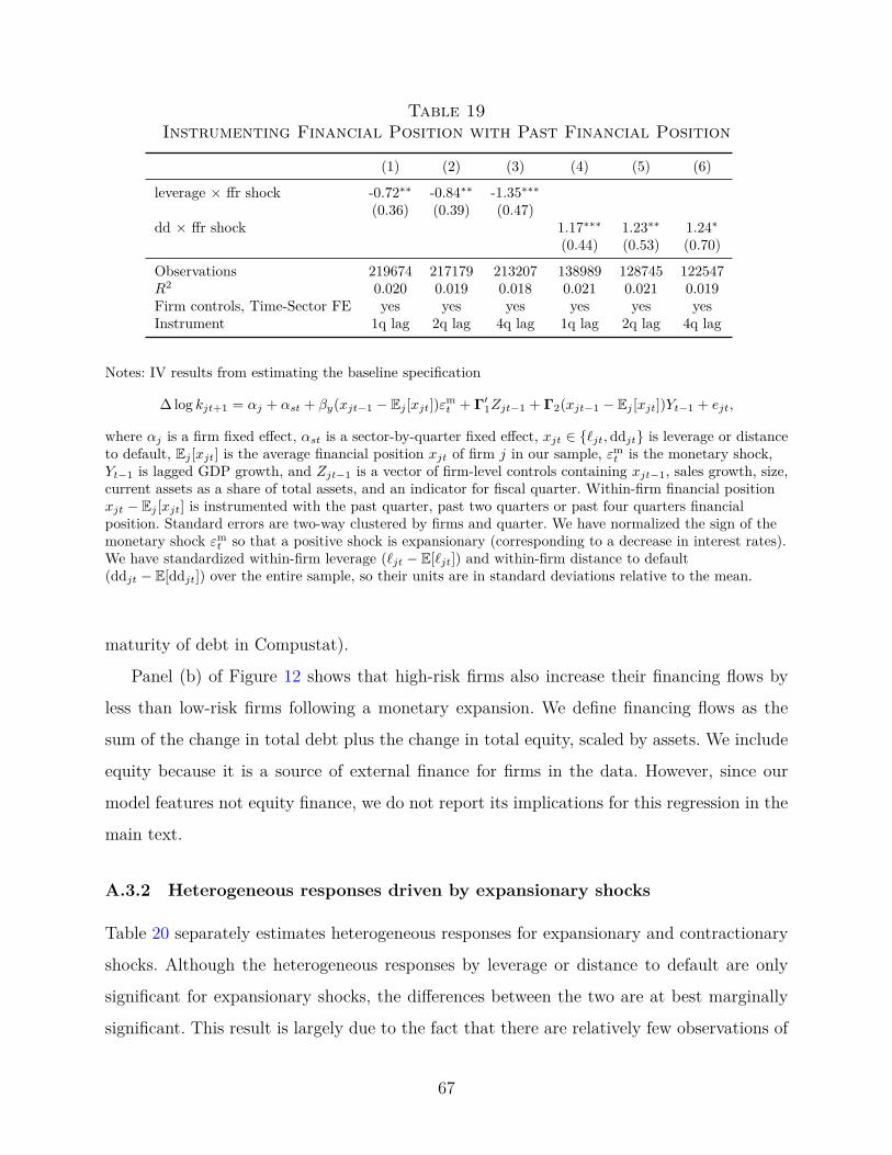
Table 19Instrumenting Financial Position with Past Financial Position

(1) (2) (3) (4) (5) (6)

leverage × ffr shock -0.72∗∗ -0.84∗∗ -1.35∗∗∗(0.36) (0.39) (0.47)

dd × ffr shock 1.17∗∗∗ 1.23∗∗ 1.24∗(0.44) (0.53) (0.70)

Observations 219674 217179 213207 138989 128745 122547R2 0.020 0.019 0.018 0.021 0.021 0.019Firm controls, Time-Sector FE yes yes yes yes yes yesInstrument 1q lag 2q lag 4q lag 1q lag 2q lag 4q lag

Notes: IV results from estimating the baseline specification

∆log kjt+1 = αj + αst + βy(xjt−1 − Ej [xjt])εmt + Γ′

1Zjt−1 + Γ2(xjt−1 − Ej [xjt])Yt−1 + ejt,

where αj is a firm fixed effect, αst is a sector-by-quarter fixed effect, xjt ∈ {ℓjt,ddjt} is leverage or distanceto default, Ej [xjt] is the average financial position xjt of firm j in our sample, εm

t is the monetary shock,Yt−1 is lagged GDP growth, and Zjt−1 is a vector of firm-level controls containing xjt−1, sales growth, size,current assets as a share of total assets, and an indicator for fiscal quarter. Within-firm financial positionxjt − Ej [xjt] is instrumented with the past quarter, past two quarters or past four quarters financialposition. Standard errors are two-way clustered by firms and quarter. We have normalized the sign of themonetary shock εm

t so that a positive shock is expansionary (corresponding to a decrease in interest rates).We have standardized within-firm leverage (ℓjt − E[ℓjt]) and within-firm distance to default(ddjt − E[ddjt]) over the entire sample, so their units are in standard deviations relative to the mean.

maturity of debt in Compustat).

Panel (b) of Figure 12 shows that high-risk firms also increase their financing flows by

less than low-risk firms following a monetary expansion. We define financing flows as the

sum of the change in total debt plus the change in total equity, scaled by assets. We include

equity because it is a source of external finance for firms in the data. However, since our

model features not equity finance, we do not report its implications for this regression in the

main text.

A.3.2 Heterogeneous responses driven by expansionary shocks

Table 20 separately estimates heterogeneous responses for expansionary and contractionary

shocks. Although the heterogeneous responses by leverage or distance to default are only

significant for expansionary shocks, the differences between the two are at best marginally

significant. This result is largely due to the fact that there are relatively few observations of

67

Table 20Expansionary vs. Contractionary Shocks

(1) (2) (3) (4)

leverage × ffr shock -0.68∗∗(0.28)

leverage × pos ffr shock -0.71∗∗(0.30)

leverage × neg ffr shock -0.56(0.96)

dd × ffr shock 1.10∗∗∗(0.39)

dd × pos ffr shock 1.38∗∗∗(0.50)

leverage × neg ffr shock 0.12(0.77)

Observations 219702 219702 151433 151433R2 0.124 0.124 0.137 0.137Firm controls yes yes yes yesTime sector FE yes yes yes yesTime clustering yes yes yes yes

Notes: results from estimating variants of the baseline specification

∆log kjt+1 = αj + αst + βy(xjt−1 − Ej [xjt])εmt + Γ′

1Zjt−1 + Γ2(xjt−1 − Ej [xjt])Yt−1 + ejt,

where αj is a firm fixed effect, αst is a sector-by-quarter fixed effect, xjt ∈ {ℓjt,ddjt} is leverage or distanceto default, Ej [xjt] is the average financial position xjt of firm j in our sample, εm

t is the monetary shock,Yt−1 is lagged GDP growth, and Zjt−1 is a vector of firm-level controls containing xjt−1, sales growth, size,current assets as a share of total assets, and an indicator for fiscal quarter. Columns (2) and (4) containseparate interactions for expansionary and contractionary shocks. Standard errors are two-way clustered byfirms and quarters. We have normalized the sign of the monetary shock εm

t so that a positive shock isexpansionary (corresponding to a decrease in interest rates). We have standardized within-firm leverage(ℓjt − E[ℓjt]) and within-firm distance to default (ddjt − E[ddjt]) over the entire sample, so their units arein standard deviations relative to the mean.

contractionary shocks in our sample, generating large standard errors.

A.3.3 Heterogeneous responses for different measures of leverage

Table 21 decomposes leverage into various types of debt and shows that our results hold for

each of these types of debt.43 In addition, the table shows that our results hold when use43This decomposition sheds light on the role of the “debt overhang” hypothesis in driving our results. Under

this hypothesis, equity holders of highly leveraged firms capture less of the return on investment; since equityholders make the investment decision, they will choose to invest less following the monetary policy shock.However, because investment is long lived, this hypothesis would predict much stronger differences by longterm debt. We find that this is not the case; if anything, the differences across firms are stronger for debtdue in less than one year.

68

Table 21Decomposition of Leverage

(1) (2) (3) (4) (5) (6) (7)

leverage × ffr shock -0.68∗∗(0.28)

net leverage × ffr shock -0.71∗∗(0.30)

ST debt × ffr shock -0.37 -0.44(0.31) (0.31)

LT debt × ffr shock -0.20 -0.35(0.25) (0.24)

other liabilities × ffr shock -0.23(0.28)

liabilities × ffr shock -0.69∗∗(0.31)

Observations 219702 219702 219702 219702 219702 219682 219682R2 0.124 0.125 0.124 0.121 0.125 0.124 0.126Firm controls yes yes yes yes yes yes yesTime sector FE yes yes yes yes yes yes yesTime clustering yes yes yes yes yes yes yes

Notes: results from estimating variants of the baseline specification

∆log kjt+1 = αj + αst + βy(xjt−1 − Ej [xjt])εmt + Γ′

1Zjt−1 + Γ2(xjt−1 − Ej [xjt])Yt−1 + ejt,

where αj is a firm fixed effect, αst is a sector-by-quarter fixed effect, xjt ∈ {ℓjt,ddjt} is leverage or distanceto default, Ej [xjt] is the average financial position xjt of firm j in our sample, εm

t is the monetary shock,Yt−1 is lagged GDP growth, and Zjt−1 is a vector of firm-level controls containing xjt−1, sales growth, size,current assets as a share of total assets, and an indicator for fiscal quarter. “Leverage” refers to leverageconstructed as in the main text. “Net leverage” is leverage net of current assets. “Short term debt” iscurrent debt (coming due in less than one year) divided by total assets. “Long term debt” is total debtminus current debt divided by total assets. “Other liabilities” is other liabilities divided by total assets.“Liabilities” is total debt plus other liabilities divided by total assets. Standard errors are two-wayclustered by firms and quarters. We have normalized the sign of the monetary shock εm

t so that a positiveshock is expansionary (corresponding to a decrease in interest rates). We have standardized within-firmleverage (ℓjt − E[ℓjt]) and within-firm distance to default (ddjt − E[ddjt]) over the entire sample, so theirunits are in standard deviations relative to the mean.

leverage net of current assets.

A.4 Comparison to Existing Literature

In this subsection, we relate our findings to empirical studies documenting heterogeneous

responses across firms with different size, age, and liquidity. Subsection A.4.1 replicates the

results of Gertler and Gilchrist (1994) regarding firm size in our sample and shows that

69

including their measure of size does not affect our results. Subsection A.4.2 replicates the

results of Cloyne et al. (2018) regarding firm age and shows that including their measure

of age also does not affect our results. Finally, subsection A.4.4 reconciles our results with

recent work by Jeenas (2018).

A.4.1 Relation to Gertler and Gilchrist (1994) and firm size

Gertler and Gilchrist (1994) showed that small firms’ sales and inventory holdings were

more sensitive to monetary contractions. In this subsection, we replicate their results in our

sample and show that they do not affect our main findings. Following Gertler and Gilchrist

(1994), we identify a small firm if their average sales over the past ten years is below the

30th percentile of the distribution.44 We then estimate our baseline dynamic model (6) using

this measure of size as the financial position xjt.

Figure 13 replicates the spirit of Gertler and Gilchrist (1994)’s results for investment

in our sample. Panel (a) measures monetary contractions as the Romer and Romer (1990)

dates in our version of Gertler and Gilchrist (1994)’s time period 1972-1989. It shows that

small firms cut investment by more than large firms following a monetary contraction. Panel

(b) show that these results also hold using our measure of monetary shocks εmt in our time

period 1990-2007, although the estimates are only marginally statistically significant.45

Figure 14 shows that our main results are unaffected by controlling for Gertler and

Gilchrist (1994)’s measure of size using the local projection:

log kjt+h − log kjt = αjh + αsth + β1h(xjt−1 − Ej[xjt])εmt + β2hsize

sjt−1ε

mt

+ Γ′1hZjt−1 + Γ2h(xjt−1 − Ej[xjt])Yt−1 + Γ3hsize

sjt−1Yt−1 + ejth. (17)

Panel (a) reports results for xjt = leverage and panel (b) reports results for xjt = distance to

default. In both cases, the dynamics of the differential response β1h are virtually identical to

the main text.46 This occurs because size and our measures of financial position are largely

uncorrelated in our sample. Hence, we view our work as simply focusing on a different feature44These results are similar if we use five or twenty year averages.45Our findings here are consistent with the analysis in Crouzet and Mehrotra (2017).46This result is robust to measuring size with capital or total assets instead of sales.

70

Figure 13: Dynamics of Differential Responses to Monetary Shocks by Size(a) Period 1972–1989 (b) Period 1990–2007

0 1 2 3 4 5 6 7 8 9 10 11 12-10

-8

-6

-4

-2

0

2

4

0 1 2 3 4 5 6 7 8 9 10 11 12-25

-20

-15

-10

-5

0

5

10

15

Notes: Estimated coefficients βh over quarters h from

log kjt+h − log kjt = αjh + αsth + βhsizesjt−1ε

mt + Γ′

1hZjt−1 + Γ′2hsize

sjt−1Yt−1 + εjth,

where αjh is a firm fixed effect, αsth is a sector-by-quarter fixed effect, sizesjt is a measure of firm sizetaking the value of one if firm j is “large” in period t and zero otherwise (see main text for definition), εm

t

is the monetary shock, Yt−1 is lagged GDP growth, and Zjt−1 is a vector of firm-level controls containingsizesjt, sales growth, current assets as a share of total assets, and an indicator for fiscal quarter. Standarderrors are two-way clustered by firm and time. Dashed lines report 90% error bands. We have normalizedthe sign of the monetary shocks εm

t so that a positive shock is expansionary (corresponding to a decrease ininterest rates). Monetary shocks in panel (a) correspond to the Romer and Romer (1990) dates.

of the data than Gertler and Gilchrist (1994).

A.4.2 Relation to Cloyne et al. (2018) and firm age

Recent work Cloyne et al. (2018) argues that younger firms are more responsive to monetary

policy in both the U.S. and the U.K. In this subsection, we replicate the spirit of their results

in our sample and show that they do not affect our main results. Following Cloyne et al.

(2018), we measure age as time since incorporating, which we download from Datastream.

Figure 15 replicates the spirit of Cloyne et al. (2018)’s results in our sample. Following

Cloyne et al. (2018), we classify firms as “young” (whose age since incorporation is less

than fifteen years), “middle aged” (between fifteen and fifty years), and “older” (more than

fifty years). Middle-aged and old firms are less responsive to monetary shocks, although

these differences are not statistically significant for most horizons in our specification and

sample.47

47A potentially important difference between our specifications is that Cloyne et al. (2018) measure mon-etary policy shocks with a VAR approach and use the high-frequency shocks as an instrumental variable.

71

Figure 14: Joint Dynamics of Financial Position and Size(a) Leverage and Size

Leverage Size

0 1 2 3 4 5 6 7 8 9 10 11 12-10

-8

-6

-4

-2

0

2

4

6

8

10

0 1 2 3 4 5 6 7 8 9 10 11 12-25

-20

-15

-10

-5

0

5

10

15

(b) Distance to Default and SizeDistance to Default Size

0 1 2 3 4 5 6 7 8 9 10 11 12-2

0

2

4

6

8

10

0 1 2 3 4 5 6 7 8 9 10 11 12-20

-15

-10

-5

0

5

10

15

20

25

Notes: Estimated coefficients β1h and β2h over quarters h from

log kjt+h − log kjt = αjh + αsth + β1h(xjt−1 − Ej [xjt])εmt + β2hsize

sjt−1ε

mt

+ Γ′1hZjt−1 + Γ′

2h(xjt−1 − Ej [xjt])Yt−1 + Γ′3hsize

sjt−1Yt−1 + ejt,

where αjh is a firm fixed effect, αsth is a sector-by-quarter fixed effect, xjt ∈ {ℓjt, dd jt} is leverage ordistance to default, sizesjt is a measure of firm size taking the value of one if firm j is “large” in period tand zero otherwise (see main text for definition), εm

t is the monetary shock, Yt−1 is lagged GDP growth,and Zjt−1 is a vector of firm-level controls containing xjt−1, sales growth, size, current assets as a share oftotal assets, and an indicator for fiscal quarter. Standard errors are two-way clustered by firms and time.Dashed lines report 90% error bands. Panel (a) runs our baseline specification with leverage xjt = ℓjt.Panel (b) runs our preferred specification with distance to default xjt = dd jt. We have normalized the signof the monetary shocks εm

t so that a positive shock is expansionary (corresponding to a decrease in interestrates). We have standardized the demeaned financial position variables xjt − Ej [xjt] and demeanedliquidity xjt − Ej [xjt] over the entire sample, so their units are in standard deviations relative to the mean.

72

Figure 15: Dynamics of Differential Responses to Monetary Shocks by Age(a) Middle-age Firms (b) Older Firms

0 1 2 3 4 5 6 7 8 9 10 11 12-15

-10

-5

0

5

10

15

0 1 2 3 4 5 6 7 8 9 10 11 12-20

-15

-10

-5

0

5

10

15

Notes: Estimated coefficients βh over quarters h from

log kjt+h − log kjt = αjh + αsth + β′hagejtε

mt + Γ′

1hZjt−1 + Γ′2hagejtYt−1 + εjth,

where αjh is a firm fixed effect, αsth is a sector-by-quarter fixed effect, agejt ≡ [middleagejt oldagejt]′ is a

vector with two dummy variables measuring firm age (see main text for definition), εmt is the monetary

shock, Yt−1 is lagged GDP growth and Zjt−1 is a vector of firm-level controls containing age, size, salesgrowth, current assets as a share of total assets, and an indicator for fiscal quarter. Panel (a) shows theinteractive coefficient associated with the variable middleagejt and Panel (b) shows oldagejt. Standarderrors are two-way clustered by firm and time. Dashed lines report 90% error bands. We have normalizedthe sign of the monetary shocks εm

t so that a positive shock is expansionary (corresponding to a decrease ininterest rates).

Figure 16 shows that our main results are robust to controlling for these measures of

firm age. We view these findings as reflecting the fact that we analyze a different dimension

of the data than Cloyne et al. (2018). We obtain similar results if we interact the monetary

shock with the level of the firm’s age rather than these coarse categories.

A.4.3 Relation to firm volatility literature

In this subsection, we explore the empirical link between firm-level volatility and the re-

sponse to monetary policy. Our motivation is a growing strand of literature that has argued

that firm-level volatility is an important determinant of how those firms respond to shocks

(see, e.g., Vavra (2013) or Bloom et al. (2015)). Indeed, one can view volatility as a proxy

for default risk, since all else equal firms with more volatile cash flows will default more

frequently. We measure volatility voljt as the standard deviation of the firm’s year-on-year

sales growth over the past twenty quarters.

Panel (a) of Figure 17 shows that firms with more volatile sales growth are less respon-

73

Figure 16: Joint Dynamics of Financial Position and Age(a) Leverage and Age

Leverage Middle-aged Firms Older Firms

0 1 2 3 4 5 6 7 8 9 10 11 12-10

-8

-6

-4

-2

0

2

4

6

8

10

0 1 2 3 4 5 6 7 8 9 10 11 12-15

-10

-5

0

5

10

0 1 2 3 4 5 6 7 8 9 10 11 12-20

-15

-10

-5

0

5

10

15

(b) Distance to Default and AgeDistance to Default Middle-aged Firms Older Firms

0 1 2 3 4 5 6 7 8 9 10 11 12-1

0

1

2

3

4

5

6

7

8

9

0 1 2 3 4 5 6 7 8 9 10 11 12-10

-8

-6

-4

-2

0

2

4

6

8

10

0 1 2 3 4 5 6 7 8 9 10 11 12-10

-5

0

5

10

15

20

Notes: Estimated coefficients β1h and β2h over quarters h from

log kjt+h − log kjt = αjh + αsth + β1h(xjt−1 − Ej [xjt])εmt + β′

2hagejtεmt

+ Γ′1hZjt−1 + Γ′

2h(xjt−1 − Ej [xjt])Yt−1 + Γ′3hagejtYt−1 + ejt,

where αjh is a firm fixed effect, αsth is a sector-by-quarter fixed effect, agejt ≡ [middleagejt oldagejt]′ is a

vector with two dummy variables measuring firm age (see main text for definition) εmt is the monetary

shock, Yt−1 is lagged GDP growth, and Zjt−1 is a vector of firm-level controls containing xjt−1, salesgrowth, size, current assets as a share of total assets, and an indicator for fiscal quarter. Standard errorsare two-way clustered by firms and time. Dashed lines report 90% error bands. Panel (a) runs our baselinespecification with leverage xjt = ℓjt. Panel (b) runs our preferred specification with distance to defaultxjt = dd jt. We have normalized the sign of the monetary shocks εm

t so that a positive shock isexpansionary (corresponding to a decrease in interest rates). We have standardized the demeaned financialposition variables xjt − Ej [xjt] and demeaned liquidity xjt − Ej [xjt] over the entire sample, so their unitsare in standard deviations relative to the mean.

74

Figure 17: Dynamics of Differential Responses to Monetary Shocks by Volatility(a) 5-year window (b) 10-year window

0 1 2 3 4 5 6 7 8 9 10 11 12-3

-2.5

-2

-1.5

-1

-0.5

0

0.5

1

1.5

2

0 1 2 3 4 5 6 7 8 9 10 11 12-8

-6

-4

-2

0

2

4

Notes: Estimated coefficients βh over quarters h from

log kjt+h − log kjt = αjh + αsth + βhvoljt−1εmt + Γ′

1hZjt−1 + Γ′2hvoljt−1Yt−1 + εjth,

where αjh is a firm fixed effect, αsth is a sector-by-quarter fixed effect, voljt is the standard deviation of thefirm’s year-on-year sales growth over the past five or ten years, εm

t is the monetary shock, Yt−1 is laggedGDP growth, and Zjt−1 is a vector of firm-level controls containing voljt, sales growth, current assets as ashare of total assets, and an indicator for fiscal quarter. Standard errors are two-way clustered by firm andtime. Dashed lines report 90% error bands. We have normalized the sign of the monetary shocks εm

t so thata positive shock is expansionary (corresponding to a decrease in interest rates). We have standardizedvolatility voljt, so their units are in standard deviations relative to the mean.

sive to monetary policy. Quantitatively, the estimates imply that a firm with one standard

deviation higher volatility has an approximately 0.5 units low semi-elasticity of investment

with respect to monetary policy. Panel (b) shows that these differential responses are larger

if we measure volatility over the past forty quarters rather than the past twenty.

However, Panel (a) of Figure 18 shows that these heterogeneous responses by volatility

become insignificant once we control for heterogeneity in distance to default. We therefore

conclude that the differences by volatility are in fact driven by differences in default risk,

consistent with our model. Panel (b) shows that controlling for leverage has a smaller effect

on the heterogeneous responses by volatility.

A.4.4 Relation to Jeenas (2018) and firm liquidity

In this subsection, we relate our findings to recent work by Jeenas (2018) along two dimen-

sions. First, we show that the differences between our estimated dynamics are accounted for

by permanent heterogeneity in responsiveness across firms. Second, we show that our results

75

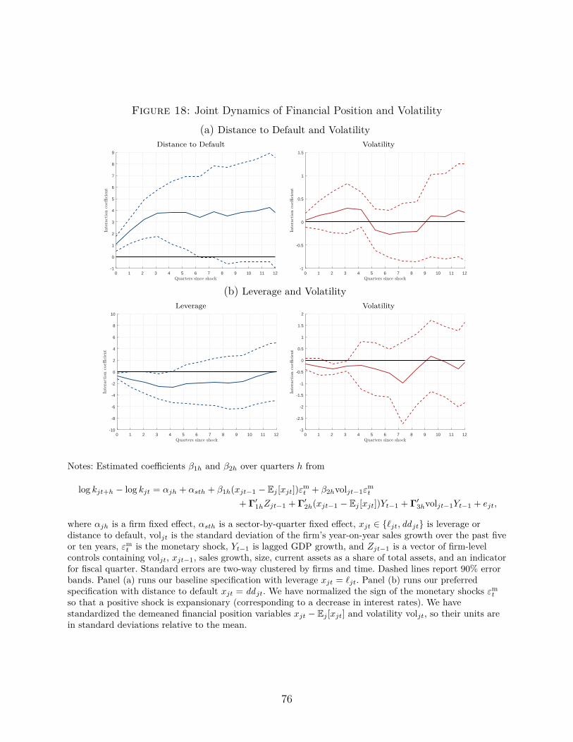
Figure 18: Joint Dynamics of Financial Position and Volatility(a) Distance to Default and Volatility

Distance to Default Volatility

0 1 2 3 4 5 6 7 8 9 10 11 12-1

0

1

2

3

4

5

6

7

8

9

0 1 2 3 4 5 6 7 8 9 10 11 12-1

-0.5

0

0.5

1

1.5

(b) Leverage and VolatilityLeverage Volatility

0 1 2 3 4 5 6 7 8 9 10 11 12-10

-8

-6

-4

-2

0

2

4

6

8

10

0 1 2 3 4 5 6 7 8 9 10 11 12-3

-2.5

-2

-1.5

-1

-0.5

0

0.5

1

1.5

2

Notes: Estimated coefficients β1h and β2h over quarters h from

log kjt+h − log kjt = αjh + αsth + β1h(xjt−1 − Ej [xjt])εmt + β2hvoljt−1ε

mt

+ Γ′1hZjt−1 + Γ′

2h(xjt−1 − Ej [xjt])Yt−1 + Γ′3hvoljt−1Yt−1 + ejt,

where αjh is a firm fixed effect, αsth is a sector-by-quarter fixed effect, xjt ∈ {ℓjt, dd jt} is leverage ordistance to default, voljt is the standard deviation of the firm’s year-on-year sales growth over the past fiveor ten years, εm

t is the monetary shock, Yt−1 is lagged GDP growth, and Zjt−1 is a vector of firm-levelcontrols containing voljt, xjt−1, sales growth, size, current assets as a share of total assets, and an indicatorfor fiscal quarter. Standard errors are two-way clustered by firms and time. Dashed lines report 90% errorbands. Panel (a) runs our baseline specification with leverage xjt = ℓjt. Panel (b) runs our preferredspecification with distance to default xjt = dd jt. We have normalized the sign of the monetary shocks εm

t

so that a positive shock is expansionary (corresponding to a decrease in interest rates). We havestandardized the demeaned financial position variables xjt − Ej [xjt] and volatility voljt, so their units arein standard deviations relative to the mean.

76

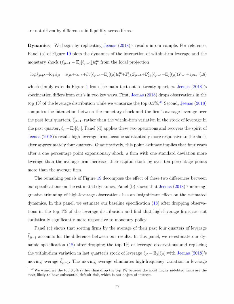
are not driven by differences in liquidity across firms.

Dynamics We begin by replicating Jeenas (2018)’s results in our sample. For reference,

Panel (a) of Figure 19 plots the dynamics of the interaction of within-firm leverage and the

monetary shock (ℓjt−1 − Ej[ℓjt−1])εmt from the local projection

log kjt+h−log kjt = αjh+αsth+βh(ℓjt−1−Ej [ℓjt])εmt +Γ′

1hZjt−1+Γ′2h(ℓjt−1−Ej [ℓjt])Yt−1+εjth, (18)

which simply extends Figure 1 from the main text out to twenty quarters. Jeenas (2018)’s

specification differs from our’s in two key ways. First, Jeenas (2018) drops observations in the

top 1% of the leverage distribution while we winsorize the top 0.5%.48 Second, Jeenas (2018)

computes the interaction between the monetary shock and the firm’s average leverage over

the past four quarters, ℓjt−1, rather than the within-firm variation in the stock of leverage in

the past quarter, ℓjt−Ej[ℓjt]. Panel (d) applies these two operations and recovers the spirit of

Jeenas (2018)’s result: high-leverage firms become substantially more responsive to the shock

after approximately four quarters. Quantitatively, this point estimate implies that four years

after a one percentage point expansionary shock, a firm with one standard deviation more

leverage than the average firm increases their capital stock by over ten percentage points

more than the average firm.

The remaining panels of Figure 19 decompose the effect of these two differences between

our specifications on the estimated dynamics. Panel (b) shows that Jeenas (2018)’s more ag-

gressive trimming of high-leverage observations has an insignificant effect on the estimated

dynamics. In this panel, we estimate our baseline specification (18) after dropping observa-

tions in the top 1% of the leverage distribution and find that high-leverage firms are not

statistically significantly more responsive to monetary policy.

Panel (c) shows that sorting firms by the average of their past four quarters of leverage

ℓjt−1 accounts for the difference between our results. In this panel, we re-estimate our dy-

namic specification (18) after dropping the top 1% of leverage observations and replacing

the within-firm variation in last quarter’s stock of leverage ℓjt −Ej[ℓjt] with Jeenas (2018)’s

moving average ℓjt−1. The moving average eliminates high-frequency variation in leverage48We winsorize the top 0.5% rather than drop the top 1% because the most highly indebted firms are the

most likely to have substantial default risk, which is our object of interest.

77

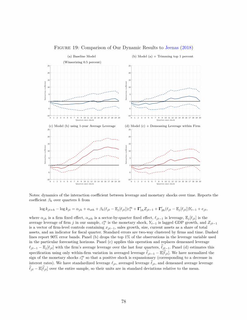
Figure 19: Comparison of Our Dynamic Results to Jeenas (2018)(a) Baseline Model (b) Model (a) + Trimming top 1 percent

(Winsorizing 0.5 percent)

0 1 2 3 4 5 6 7 8 9 10 11 12 13 14 15 16 17 18 19 20-10

-5

0

5

10

15

20

25

0 1 2 3 4 5 6 7 8 9 10 11 12 13 14 15 16 17 18 19 20-10

-5

0

5

10

15

20

25

(c) Model (b) using 1-year Average Leverage (d) Model (c) + Demeaning Leverage within Firm

0 1 2 3 4 5 6 7 8 9 10 11 12 13 14 15 16 17 18 19 20-10

-5

0

5

10

15

20

25

0 1 2 3 4 5 6 7 8 9 10 11 12 13 14 15 16 17 18 19 20-10

-5

0

5

10

15

20

25

Notes: dynamics of the interaction coefficient between leverage and monetary shocks over time. Reports thecoefficient βh over quarters h from

log kjt+h − log kjt = αjh + αsth + βh(ℓjt − Ej [ℓjt])εmt + Γ′

1hZjt−1 + Γ′2h(ℓjt − Ej [ℓjt])Yt−1 + ejt,

where αjh is a firm fixed effect, αsth is a sector-by-quarter fixed effect, ℓjt−1 is leverage, Ej [ℓjt] is theaverage leverage of firm j in our sample, εm

t is the monetary shock, Yt−1 is lagged GDP growth, and Zjt−1

is a vector of firm-level controls containing xjt−1, sales growth, size, current assets as a share of totalassets, and an indicator for fiscal quarter. Standard errors are two-way clustered by firms and time. Dashedlines report 90% error bands. Panel (b) drops the top 1% of the observations in the leverage variable usedin the particular forecasting horizons. Panel (c) applies this operation and replaces demeaned leverageℓjt−1 − Ej [ℓjt] with the firm’s average leverage over the last four quarters, ℓjt−1. Panel (d) estimates thisspecification using only within-firm variation in averaged leverage ℓjt−1 − E[ℓjt]. We have normalized thesign of the monetary shocks εm

t so that a positive shock is expansionary (corresponding to a decrease ininterest rates). We have standardized leverage ℓjt, averaged leverage ℓjt, and demeaned average leverageℓjt − E[ℓjt] over the entire sample, so their units are in standard deviations relative to the mean.

78

within a firm, implying that the estimated dynamics are more strongly driven by perma-

nent heterogeneity across firms. Consistent with this idea, Panel (d) shows that using only

within-firm variation in averaged leverage ℓjt−1 − Ej[ℓjt] renders the long-horizon dynamics

smaller and significantly insignificant, largely consistent with our baseline specification. We

prefer our specification because it maps more directly into our economic model in which het-

erogeneity in leverage is driven by ex-post realizations of idiosyncratic shocks and lifecycle

dynamics across firms. We focus our analysis of the model on the heterogeneous responses

upon impact, which are robustly estimated in both our specification and Jeenas (2018) and

survive the litany of robustness checks in Appendices A.2 and A.3.49

Heterogeneous Responses Not Driven by Liquidity Jeenas (2018) argues that the

dynamics of heterogeneous responses by leverage documented above are driven by differences

in liquidity across firms. Table 18 above shows that the heterogeneous responses upon impact

are not driven by liquidity once we use within-firm variation in our main specification (5).

Figure 20 shows that our dynamics results are not driven by differences in liquidity either.

We estimate the local projection

log kjt+h − log kjt = αjh + αsth + β1h(xjt−1 − Ej[xjt])εmt + β2h(yjt−1 − Ej[yjt])ε

mt (19)

+ Γ′1hZjt−1 + Γ2h(xjt−1 − Ej[xjt])Yt−1 + Γ3h(yjt−1 − Ej[yjt])Yt−1 + ejth,

where yjt − Ej[yjt] is the within-firm variation in liquidity. Panel (a) shows that the point

estimate of the leverage dynamics are similar to those presented in the main text, although

the standard errors are wider given the correlation between leverage and liquidity. Panel (b)

shows that the dynamics of distance to default are strongly and significantly positive, as in

the main text. In that case, the dynamics of liquidity are always statistically insignificant,49An additional difference between our specification and Jeenas (2018)’s is that we control for differences

in cyclical sensitivities while Jeenas (2018) does not. We include these controls because we have found thatthere are significant differences in long-run cyclical sensitivities and that GDP growth is correlated withmonetary shocks over these horizons in our sample. Appendix A.3 shows that excluding these controls doesnot affect the point estimates in our specification but does increase the standard errors. We have also foundthat excluding these controls does not strongly affect the point estimates or standard errors in Jeenas (2018)’sbaseline specification with averaged leverage ℓjt. Excluding these controls slightly increases the responsivenessof high demeaned average leverage firms ℓjt −Ej [ℓjt], but the difference from Panel (d) in Figure 19 is smalland not statistically significant.

79

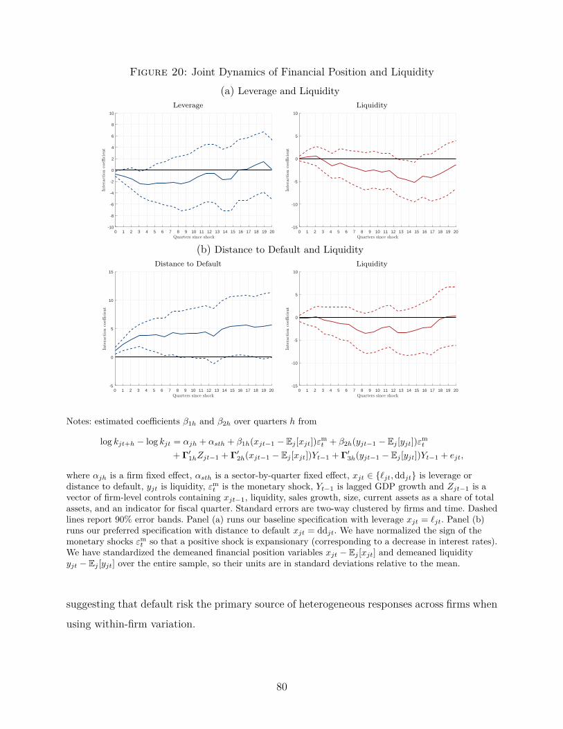
Figure 20: Joint Dynamics of Financial Position and Liquidity(a) Leverage and Liquidity

Leverage Liquidity

0 1 2 3 4 5 6 7 8 9 10 11 12 13 14 15 16 17 18 19 20-10

-8

-6

-4

-2

0

2

4

6

8

10

0 1 2 3 4 5 6 7 8 9 10 11 12 13 14 15 16 17 18 19 20-15

-10

-5

0

5

10

(b) Distance to Default and LiquidityDistance to Default Liquidity

0 1 2 3 4 5 6 7 8 9 10 11 12 13 14 15 16 17 18 19 20-5

0

5

10

15

0 1 2 3 4 5 6 7 8 9 10 11 12 13 14 15 16 17 18 19 20-15

-10

-5

0

5

10

Notes: estimated coefficients β1h and β2h over quarters h from

log kjt+h − log kjt = αjh + αsth + β1h(xjt−1 − Ej [xjt])εmt + β2h(yjt−1 − Ej [yjt])ε

mt

+ Γ′1hZjt−1 + Γ′

2h(xjt−1 − Ej [xjt])Yt−1 + Γ′3h(yjt−1 − Ej [yjt])Yt−1 + ejt,

where αjh is a firm fixed effect, αsth is a sector-by-quarter fixed effect, xjt ∈ {ℓjt,ddjt} is leverage ordistance to default, yjt is liquidity, εm

t is the monetary shock, Yt−1 is lagged GDP growth and Zjt−1 is avector of firm-level controls containing xjt−1, liquidity, sales growth, size, current assets as a share of totalassets, and an indicator for fiscal quarter. Standard errors are two-way clustered by firms and time. Dashedlines report 90% error bands. Panel (a) runs our baseline specification with leverage xjt = ℓjt. Panel (b)runs our preferred specification with distance to default xjt = ddjt. We have normalized the sign of themonetary shocks εm

t so that a positive shock is expansionary (corresponding to a decrease in interest rates).We have standardized the demeaned financial position variables xjt − Ej [xjt] and demeaned liquidityyjt − Ej [yjt] over the entire sample, so their units are in standard deviations relative to the mean.

suggesting that default risk the primary source of heterogeneous responses across firms when

using within-firm variation.

80

B Model Appendix

B.1 Proof of Proposition 1

We prove Proposition 1 in steady state; extending the proof to include transition dynamics

is straightforward. To clarify the economic mechanisms, we work with a simple version of the

model that abstracts from capital-quality shocks (σω = 0), has zero recovery value of debt

(α = 0), and has no exogenous exit shocks (πd = 0). The proof in the full model follows the

same steps with more complicated notation.

Default Threshold As discussed in the main text, firms only default when they have no

feasible choice which satisfies the non-negativity constraint on dividends, i.e., there is no

(k′, b′) such that n− k′ +Q(z, k′, b′)b′ ≥ 0. Define the default threshold n(z) = mink′,b′ k′ −

Q(z, k′, b′)b′. Note that the largest feasible dividend payment of a firm is n−x(z). If n ≥ n(z),

then argmink′,b′ k′ − Q(z, k′, b′)b′ is a feasible choice and the firm will not default. On the

other hand, if n < n(z), then d ≤ 0 for all (k′, b′), violating feasibility.

With this notation in hand, the Bellman equation of a continuing firm in this simple case

is

v(z, n) = maxk′,b′

n− k′ +Q(z, k′, b′)b′ + βE [v(z′, n′)1{n′ > n(z′)}|z, k′, b′] s.t. d ≥ 0, (20)

where n(z′) is the default threshold.

Although the continuation value is kinked at the default point, it is never optimal for a

firm to choose this point (see Clausen and Strub (2017) and the discussion in Arellano et al.

(2016)). Hence, the first order conditions are necessary at the optimum.

Unconstrained Firms Define the unconstrained capital accumulation rule k∗(z) as

k∗(z) = argmaxk′

−k′ + βE [ι(z′, k′) + (1− δ)k′|z] ,

where ι(z, k) = maxl zkθlν −wl. After some algebra, one can show that the expression in the

main text solves this maximization problem (extending the expression to the full model).

81

We will now fully characterize the decision rules for firms that can afford the uncon-

strained capital accumulation rule while have zero probability of default in all future states.

We first claim that such a firm is indifferent over any choice of debt b′ which leaves the firm

unconstrained. To show this, note that since the firm has no default risk it borrows at the

risk-free rate β. In this case, the first order condition for borrowing b′ is β = β, which is

obviously true for any value of b′.

Following Khan, Senga and Thomas (2016), we resolve this indeterminacy by defining the

maximum borrowing policy b∗(z) as the maximal borrowing b′ the firm can do while having

zero probability of default in all future states.50 To derive the maximum borrowing policy

b∗(z), first note that if the firm if the firm invests k∗(z) and borrows b∗(z) in the current

period, its dividends in the next period are

ι(z′, k∗(z)) + (1− δ)k∗(z)− b∗(z)− ξ − k∗(z′) + βb∗(z′),

for a given realization of z′. The requirement that the firm has zero probability of default in

all future states then implies that

b∗(z) = minz′

ι(z′, k∗(z)) + (1− δ)k∗(z)− k∗(z′) + βb∗(z′).

Hence, b∗(z) is the largest amount of borrowing the firm can do and be guaranteed to satisfy

the non-negativity constraint on dividends.51

By construction, if a firm can follow the unconstrained capital accumulation policy k∗(z)

and the maximum borrowing policy b∗(z) while satisfying the non-negativity constraint on

dividends in the current period, it will also satisfy the non-negativity constraint in all future

periods. Moreover, following k∗(z) is indeed optimal for such firms because it solves the

associated first-order condition of these firms. Hence, a firm is unconstrained and follows50Khan, Senga and Thomas (2016) refer to this object as the “minimum savings policy.”51To derive this expression, first re-arrange the non-negativity constraint on dividends conditional on

a realization of the future shocks as an inequality with b′ on the left-hand side. This results in a set ofinequalities for each possible realization of the future shocks. The min operator ensures that all of theseinequalities are satisfied.

82

these decision rules if and only if d = n− k∗(z) + βb∗(z), i.e.,

n > n(z) ≡ k∗(z)− βb∗(z).

Constrained Firms Consider again the constrained Bellman equation (20). We will show

that firms with n ∈ [n(z), n(z)] pay zero dividends. Invert the default threshold n(z) so that

the firm defaults if z′ < z(k′, b′). The Bellman equation (20) can then be written as

v(z, n) = maxk′,b′

n− k′ +Q(z, k′, b′)b′ + β

∫ z

z(k′,b′)

v(z′, n′)g(z′|z)dz′ s.t. d ≥ 0, (21)

where g(z′|z) is the density of z′ conditional on z, z is the upper bound of the support of z,

and Q3(z, k′, b′) is the derivative of the debt price schedule with respect to b′.

Letting λ(z, n) be the Lagrange multiplier on the d ≥ 0 constraint, the first order condi-

tion for b′ is

(1 + λ(z, n))(Q(z, k′, b′) +Q3(z, k′, b′)b′) =

β

[∫ z

z(k′,b′)

(1 + λ(z′, k′, b′)g(z′|z)dz′ + g(z(k′, b′)|z)v(z(k′, b′), n′(k′, b′))∂z(k′, b′)

∂b′

],

where n′(k′, b′) = maxn′ z(k′, b′)(k′)θ(n′)ν −wn′+(1− δ)k′− b′− ξ and λ(z′, k′, b′) = λ(z′, n′)

for the n′ implied by (z′, k′, b′). The left hand side of this expression measures the marginal

benefit of borrowing. The marginal resources the firm receives on borrowing is the debt price,

adjusting for the fact that the marginal cost of borrowing changes on existing debt. The firm

values those marginal resources using the Lagrange multiplier. The right hand side of this

expression measures the discounted marginal cost of borrowing. In states of the world in

which the firm does not default, it must give up one unit of resources, which it values using

the next period’s Lagrange multiplier. In addition, marginal borrowing implies that the firm

defaults in additional future states.

Note that the debt price schedule is Q(z, k′, b′) = β∫ z

z(k′,b′)g(z′|z)dz′, which implies that

83

Q3(z, k′, b′) = −βg(z(k′, b′)|z)∂z(k

′,b′)∂b′

. Plugging this into the first order condition gives

β(1 + λ(z, n))(

∫ z

z(k′,b′)

g(z′|z)dz′ − βg(z(k′, b′)|z)∂z(k′, b′)

∂b′=

β

[∫ z

z(k′,b′)

(1 + λ(z′, k′, b′)g(z′|z)dz′ + g(z(k′, b′)|z)v(z(k′, b′), n′(k′, b′))∂z(k′, b′)

∂b′

]. (22)

We will now show that constrained firms set d = 0. We do so by contradiction: suppose

that a constrained firm sets d > 0, implying that λ(z, n) = 0.

First consider a firm that has zero probability of default in the next period, i.e., z(k′, b′) =

z and ∂z(k′,b′)∂b′

= 0. In this case, the first order condition (22) can be simplified to

0 =

∫ z

z

λ(z′, k′, b′)g(z′|z)dz′.

Since the firm is constrained, λ(z′, k′, b′) > 0 for some positive mass of realizations of z′,

leading to a contradiction.

Now consider a firm that has some positive probability of default, implying that z(k′, b′) >

z and ∂z(k′,b′)∂b′

> 0. In this case, the first order condition (22) can be rearranged to

0 =

∫ z

z(k′,b′)

λ(z′, k′, b′)g(z′|z)dz′ + ∂z(k′, b′)

∂b′g(z(k′, b′)|z)(b′ + v(z′, k′, b′)),

where v(z′, k′, b′) = v(z′, x′) for the x′ implied by (z′, k′, b′). By construction, risky constrained

firms engage in strictly positive borrowing b′ > 0. This implies that the right hand side is

strictly greater than zero, leading to a contradiction.

B.2 Equilibrium Definition

Distribution of Firms We need to derive the evolution of the distribution of firms in

order to precisely define an equilibrium. The distribution of firms in production is composed

of incumbents who do not default and new entrants who do not default. Mathematically,

84

this distribution µt(z, n) is given by

µt(z, n) =

∫ (πdχ

1(nt(z, ω, k, b)) + (1− πd)χ2t (z, nt(z, ω, k, b))

)dµt(z, ω, k, b) (23)

+ µt

∫ (πdχ

1(nt(z, ω, k0, 0)) + (1− πd)χ2t (z, nt(z, ω, k0, 0))

)g(ω)dωdµent(z),

where nt(z, ω, k, b) = maxl ptz(ωk)θlν − wtl + qt(1− δ)ωk − b− ξ is the implied net worth x

of a firm with state (z, ω, k, b) and g(ω) is the p.d.f. of capital quality shocks.

The evolution of the distribution of firms µt(z, ω, k, b) is given by

µt+1(z′, ω′, k′, b′) =

∫(1− πd)χ

2t (z, nt(z, ω, k, b))1{k′

t(z, nt(z, ω, k, b)) = k′} (24)

× 1{b′t(z, nt(z, ω, k, b))

Πt+1

= b′}p(ε|eρ log z+ε = z′)g(ω′)dεdµt(z, ω, k, b)

+ µt

∫(1− πd)χ

2t (z, nt(z, ω, k0, 0))1{k′

t(z, nt(z, ω, k0, 0)) = k′}

× 1{b′t(z, nt(z, ω, k0, 0))

Πt+1

= b′}p(ε|eρ log z+ε = z′)g(ω′)dεdµent(z),

where p(ε|eρ log z+ε = z′) denotes the density of draws ε such that eρ log z+ε = z′.

Equilibrium Definition An equilibrium of this model is a set of vt(z, n), k′t(z, n),

b′t(z, n), nt(z, n), Qt(z, k′, b′), Πt, ∆t, Yt, qt, µt(z, ω, k, b), µt(z, n), Λt,t+1, wt, Ct, and It such

that

(i) Production firms optimization: vt(z, n) solves the Bellman equation (9) with associated

decision rules k′t(z, n), b′t(z, n), and nt(z, n).

(ii) Financial intermediaries price default risk according to (10).

(iii) New Keynesian block: Πt, pt, and qt satisfy (11) and (13).

(iv) The distribution of firms in production µt(z, n) satisfies (23) and the distribution

µt(z, ω, k, b) evolves according to (24).

(v) Household block: the stochastic discount factor is given by Λt,t+1 = βC−σ

t+1

C−σt

. The wage

must satisfy wt = ΨCt. The stochastic discount factor and nominal interest rate are

85

linked through the Euler equation for bonds, 1 = Et

[Λt,t+1

Rnomt

Πt+1

].

(vi) Market clearing: aggregate investment is implicitly defined by Kt+1 = Φ( ItKt)Kt +

(1 − δ)Kt, where Kt =∫kdµt(z, ω, k, b). Aggregate consumption is defined by Ct =

Yt − It − ξ.52

B.3 Analysis of Calibrated Model

In this appendix, we analyze firms’ decision rules in our calibrated steady state and show

that the financial heterogeneity in our model is broadly comparable to that in the data.

Identification of Fitted Parameters Figure 21 reports information to help assess the

sources of identification in our calibration exercise. The top panel reports the local elasticities

of targeted moments with respect to the parameter chosen in our calibration, computed at

the estimated parameters. The patterns which emerge are intuitive. For example, increasing

the volatility of productivity shocks σ increases the dispersion of investment rates across firms

but decreases default rates and leverage ratios (because it makes right-tail positive outcomes

more likely). In contrast, increasing the volatility of capital quality shocks makes left-tail

negative outcomes more likely and therefore increases default rates (consistent with our

discussion in Footnote 16). Increasing the operating cost ξ or decreasing lenders’ recovery

rates α tightens the financial constraints and leads to higher default rates among firms.

Finally, increasing the initial size of new firms k0 or their productivity m makes default less

likely/

The bottom panel of Figure 21 plots the inverse of the mapping in the top panel, i.e., it

plots the local elasticities of estimated parameters with respect to moments as in Andrews,

Gentzkow and Shapiro (2017). This inverse mapping clarifies how variation in targeted mo-

ments would influence estimated parameter values, taking into account the joint dependencies

across moments in the data. An important limitation of this exercise is that the relevant size

of the variation in the moments is not clear; nevertheless, we believe it contains additional

useful information. For example, it shows that the dispersion of investment rates across firms52We normalize the mass of firms in production to 1, so ξ is the total resources lost from the fixed operating

costs.

86

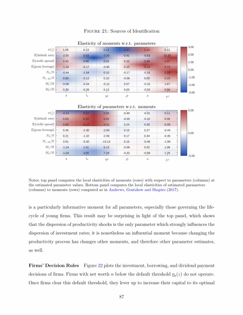
Figure 21: Sources of Identification

1.05

-2.55

2.42

-1.26

-0.44

0.50

-0.06

0.39

0.13

0.63

0.86

-0.17

-1.04

-0.12

-0.34

-0.26

0.13

-3.30

0.02

-0.90

0.10

0.10

-0.12

0.12

-2.57

0.41

0.10

0.10

-0.17

-0.06

0.07

0.03

2.10

-0.63

3.48

-0.14

-0.16

0.00

-0.10

-0.03

0.11

15.30

1.47

3.73

1.23

0.15

1.67

0.56-3.00

-2.00

-1.00

0.00

1.00

2.00

3.00

-0.14

0.03

0.06

0.35

0.21

3.91

-1.24

-1.04

0.27

0.22

-0.17

-1.30

-1.32

-5.30

1.41

3.00

0.60

0.02

-0.31

-2.60

-2.06

-13.14

6.13

7.29

-0.40

-0.05

0.24

0.15

0.17

0.16

-0.06

-0.32

-0.01

-0.10

0.30

0.27

0.34

-0.48

0.02

-0.58

0.11

0.06

-0.05

-0.44

-0.35

-1.99

1.08

1.25-5.00

0.00

5.00

Notes: top panel computes the local elasticities of moments (rows) with respect to parameters (columns) atthe estimated parameter values. Bottom panel computes the local elasticities of estimated parameters(columns) to moments (rows) computed as in Andrews, Gentzkow and Shapiro (2017).

is a particularly informative moment for all parameters, especially those governing the life-

cycle of young firms. This result may be surprising in light of the top panel, which shows

that the dispersion of productivity shocks is the only parameter which strongly influences the

dispersion of investment rates; it is nonetheless an influential moment because changing the

productivity process has changes other moments, and therefore other parameter estimates,

as well.

Firms’ Decision Rules Figure 22 plots the investment, borrowing, and dividend payment

decisions of firms. Firms with net worth n below the default threshold nt(z) do not operate.

Once firms clear this default threshold, they lever up to increase their capital to its optimal

87

Figure 22: Steady State Decision Rules

Notes: Left panel plots decision rules and stationary distribution of firms conditional on idiosyncraticproductivity one standard deviation below the mean. Right panel plots the same objects conditional onproductivity one standard deviation above the mean. The left y-axis measures the decision rules (capitalaccumulation, borrowing, and dividend payments) as a function of net worth n. The right y-axis measuresthe stationary distribution of firms (dashed purple line).

scale k∗t (z). Once capital is at its optimal level k∗

t (z), firms use additional net worth to pay

down their debt until they reach the unconstrained threshold nt(z). Only unconstrained firms

pay positive dividends.

The curvature in the policy functions over the region with low net worth n reflects the

role of financial frictions in firms’ decisions. Without frictions, all non-defaulting firms would

borrow the amount necessary to reach the optimal scale of capital k∗t (z). However, firms with

low net worth n would need to borrow a substantial amount in order to do so, increasing

their risk of default and therefore borrowing costs. Anticipating these higher borrowing costs,

low net worth n firms accumulate capital below its optimal scale.

The right axis of Figure 22 plots the stationary distribution of firms. 53.5% of firms

pay a risk premium, i.e., are “risky constrained.” These firms are in the region with curved

policy functions described above. 45.8% of firms are constrained but do not currently pay

a risk premium, i.e., are “risk-free constrained.” These firms have achieved their optimal

scale of capital k∗t (z) and have linear borrowing policies. The remaining 0.6% of firms are

unconstrained.

Figure 22 makes clear that there are two key sources of financial heterogeneity in the

88

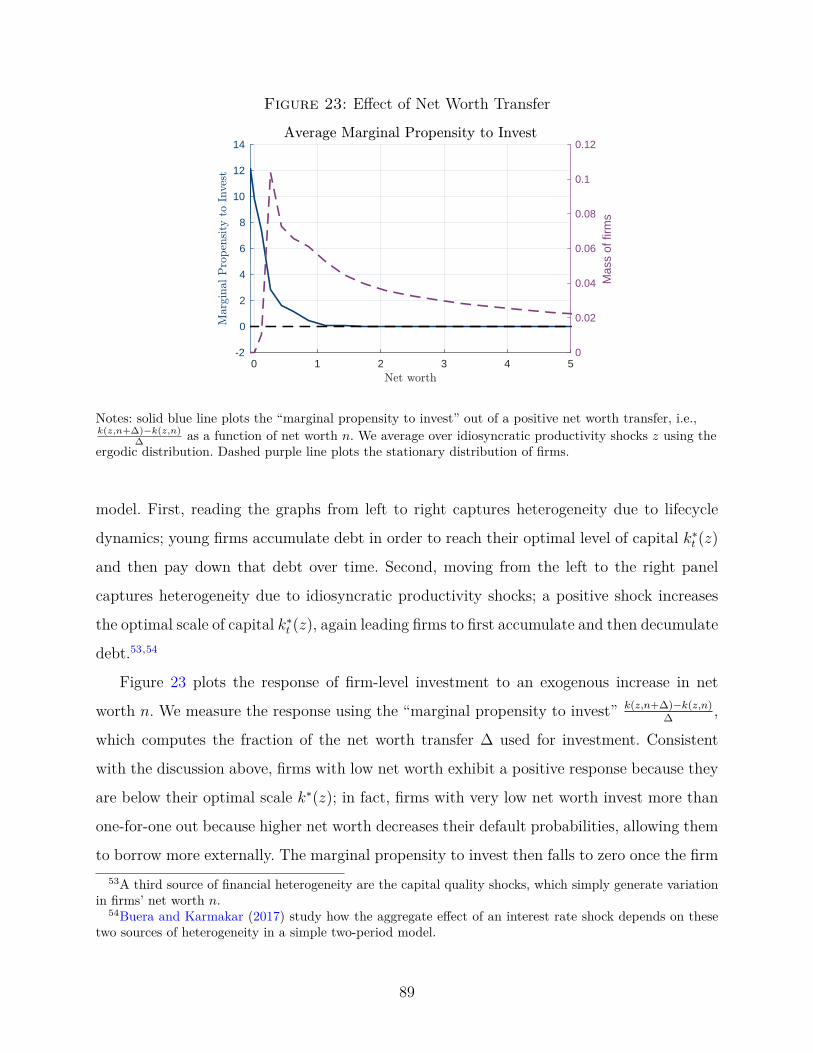
Figure 23: Effect of Net Worth Transfer

0 1 2 3 4 5-2

0

2

4

6

8

10

12

14

0

0.02

0.04

0.06

0.08

0.1

0.12

Mas

s of

firm

s

Notes: solid blue line plots the “marginal propensity to invest” out of a positive net worth transfer, i.e.,k(z,n+∆)−k(z,n)

∆ as a function of net worth n. We average over idiosyncratic productivity shocks z using theergodic distribution. Dashed purple line plots the stationary distribution of firms.

model. First, reading the graphs from left to right captures heterogeneity due to lifecycle

dynamics; young firms accumulate debt in order to reach their optimal level of capital k∗t (z)

and then pay down that debt over time. Second, moving from the left to the right panel

captures heterogeneity due to idiosyncratic productivity shocks; a positive shock increases

the optimal scale of capital k∗t (z), again leading firms to first accumulate and then decumulate

debt.53,54

Figure 23 plots the response of firm-level investment to an exogenous increase in net

worth n. We measure the response using the “marginal propensity to invest” k(z,n+∆)−k(z,n)∆

,

which computes the fraction of the net worth transfer ∆ used for investment. Consistent

with the discussion above, firms with low net worth exhibit a positive response because they

are below their optimal scale k∗(z); in fact, firms with very low net worth invest more than

one-for-one out because higher net worth decreases their default probabilities, allowing them

to borrow more externally. The marginal propensity to invest then falls to zero once the firm53A third source of financial heterogeneity are the capital quality shocks, which simply generate variation

in firms’ net worth n.54Buera and Karmakar (2017) study how the aggregate effect of an interest rate shock depends on these

two sources of heterogeneity in a simple two-period model.

89

Figure 24: Relationship between leverage and net worth

1 2 3 4 5Net worth

-0.5

0

0.5

1

1.5

Leverage

b′

k′

0.02

0.04

0.06

0.08

0.1

0.12

Mas

s of

firm

s

Notes: firms’ optimal leverage choice b′(z,n)k′(z,n) as a function of net worth in steady state. We average over

idiosyncratic productivity z using its ergodic distribution.

reaches its optimal scale k∗(z). The average marginal propensity to invest in steady state is

approximately 0.17.

Finally, Figure 24 shows that there is a strong a monotonic relationship between firms’

leverage and net worth in our model. Given that firms only default when net worth is below

the threshold n(z), this figure implies that there is a monotonically increasing relationship

between leverage and default risk in our model.

Lifecycle Dynamics Figure 25 plots the dynamics of key variables over the firm lifecy-

cle. New entrants begin with a low initial capital stock k0 and, on average, a low draw of

idiosyncratic productivity z. As described above, young firms take on new debt in order to

finance investment, which increases their default risk and credit spreads. Over time, as firms

accumulate capital and productivity reverts to its mean, they reach their optimal capital

stock k∗t (z) and begin paying down their debt.

Investment and Leverage Heterogeneity in the Data Table 22 shows that our model

is broadly consistent with key features of the distributions of investment and leverage not

targeted in the calibration. The top panel analyzes the distribution of investment rates

in the annual Census data reported by Cooper and Haltiwanger (2006). We present the

90

Figure 25: Lifecycle Dynamics in Model

10 20 30 40 500

2

4

6

Cap

ital

10 20 30 40 50-1

0

1

2

Deb

t

10 20 30 40 50-0.5

0

0.5

1

1.5

Leve

rage

10 20 30 40 500.85

0.9

0.95

1

1.05

Pro

duct

ivity

10 20 30 40 500

0.2

0.4

0.6

0.8

Em

ploy

men

t

10 20 30 40 500

2

4

6

8

Ann

ualiz

ed p

.p.

Notes: Average capital, debt, leverage, productivity, employment, and credit spread conditional on age insteady state.

corresponding statistics in our model for a selected sample – conditioning on firms that

survive at least twenty years to mirror the selection into the LRD – and in the full sample.

Although we have calibrated the selected sample to match the dispersion of investment rates,

the mean and autocorrelation of investment rates in the selected sample are also reasonable.

The mean investment rate in the full sample is higher than the selected sample because the

full sample includes young, growing firms.

The bottom panel of Table 22 compare the model-implied distribution of investment rates

and leverage to quarterly Compustat data. We mirror the sample selection into Compustat

by conditioning on firms that survive for at least ten years. According to Wilmer et al.

(2017), the median time to IPO has ranged from roughly six to eight years over the last

decade.55 Our model provides a close match of the persistence of leverage and its correlation

with investment in the selected sample.

Table 23 shows that the model generates a positive measured investment-cash flow sensi-55Our results are robustness to sensitivity analysis around this cutoff.

91

Table 22Investment and Leverage Heterogeneity

Moment Description Data Model Model(selected) (full)

Investment heterogeneity (annual LRD)E[ik

]Mean investment rate 12.2% 9.59% 22.3%

σ(ik

)SD investment rate (calibrated) 33.7% 31.8% 44.8%

ρ(

ik, ik−1

)Autocorr investment rate 0.058 -0.16 -0.16

Joint investment and leverage heterogeneity (quarterly Compustat)ρ(

bk, bk−1

)Autocorr leverage ratio 0.94 0.95 0.09

ρ(ik, bk

)Corr. of leverage and investment -0.08 -0.10 -0.20

Notes: Statistics about the cross-sectional distribution of investment rates and leverage ratios in steadystate. Data for investment heterogeneity are drawn from Cooper and Haltiwanger (2006). Model (selected)for investment heterogeneity corresponds to firms alive for longer than twenty years in a panel simulation,time aggregated to the annual frequency. Model (full) corresponds to the full sample of firms in a panelsimulation, time aggregated to the annual frequency. Data for joint investment and leverage heterogeneitydrawn from quarterly Compustat data. Model (selected) for leverage heterogeneity corresponds to firmsalive for longer than ten years in a panel simulation. Model (full) corresponds to the full sample of firms ina panel simulation.

tivity, consistent with the data. Following Gomes (2001), we compute investment-cash flow

sensitivity using the regression

ijtkjt

= a1CFjt−1

kjt+ a2qjt−1 + εjt, (25)

where CFjt is cash flow and qjt is Tobin’s q. The coefficient a1 captures the statistical co-

movement of investment with cash flow, conditional on the fixed effects and Tobin’s q. In

the model, we identify cash flow as the firm’s flow profits maxl zjt(ωjtkjt)θlνjt − wtl and To-

bin’s q as the ratio of market value to the book value of capital, k. In quarterly Compustat,

we identify cash flow as earnings before tax, depreciation, and amortization (EBITDA) and

Tobin’s q as the market to book value of the firm.

Compustat Firms in the Model and the Data Table 24 compares public and private

firms in our model to the data along three key dimensions. First, public firms are substantially

larger than private firms in our model; however, our model comes nowhere close to the size

gap observed in the data. An important reason for this discrepancy is that, in the data,

92

Table 23Measured Investment-Cash Flow Sensitivity

Without cash flow With cash flowData Model Data Model

Tobin’s q 0.01*** 0.01 0.01*** 0.01cash flow 0.02*** 0.07

Notes: Results from estimating the regression (25). Data refers to quarterly Compustat data. We measurecash flow as earnings before tax, depreciation, and amortization (EBITDA) and Tobin’s q as the market tobook value of the firm. Model refers to simulating a panel of firms from the calibrated model, conditionalon surviving at least ten years. We measure cash flow as the firm’s flow profits maxl zjt(ωjtkjt)

θlνjt − wtland Tobin’s q as the ratio of market value to the book value of capital, k.

Table 24Public vs. private firms in the model and data

Data ModelE[n|public]E[n|private] 62 1.53E[age|public]E[age|private] 2.18 3.28σ( 1

2

njt−njt−1njt+njt−1

|public)

σ( 12

njt−njt−1njt+njt−1

|private)0.58 0.62

Notes: comparison of public and private firms. “Public” firms in the model are those who reach 10 years old(the median time to IPO in Wilmer et al. (2017)). E[n|public]

E[n|private] computes the average size of firms measuredby employment; data comes from Dinlersoz et al. (2018b) Table 3. E[age|public]

E[age|private] computes the average age;

data comes from Dinlersoz et al. (2018b) Table 3.σ( 1

2

njt−njt−1njt+njt−1

|public)

σ( 12

njt−njt−1njt+njt−1

|private)computes the dispersion of growth

rates; data comes from Davis et al. (2006) Figure 2.5.

many firms are born small and never grow; therefore, there is a large mass of permanently

small firms which is outside of our model.56 Second, public firms are older than private firms

in both our model and the data; the gap is larger in our model since we select firms based

solely on age. Finally, the dispersion of growth rates is smaller among public firms in both

the model and data. In our model, private firms’ growth rates are more disperse since they56Gavazza, Mongey and Violante (2018) use permanent heterogeneity in returns to scale to match this

group of permanently small firms. We have solved a related version of our model in which there are twotypes firms: one with low returns to scale, which reach their optimal size relative quickly, and another withthe returns to scale of our baseline model. This model generates a skewed size distribution, as in the data,but by construction does not directly affect the behavior of the large “Compustat” firms in our model. Inaddition, these small firms make up a small share of aggregate investment and are therefore unlikely to havea substantial influence on aggregate dynamics.

93

are more strongly affected by financial frictions.

94