Financial frictions in a DSGE model for Latvia

Dynare Working Papers Serieshttp://www.dynare.org/wp/

Financial frictions in a DSGE model for Latvia

Buss Ginters

Working Paper no. 42

May 2015

142, rue du Chevaleret — 75013 Paris — Francehttp://www.cepremap.fr

http://www.dynare.org/wp/

http://www.cepremap.fr

Financial frictions in a DSGE model for Latvia∗

Ginters Buss†

Bank of Latvia

September 17, 2014

Abstract

This paper builds a dynamic stochastic general equilibrium (DSGE) model forLatvia that would be suitable for policy analysis and forecasting purposes at Bankof Latvia. For that purpose, I adapt the DSGE model with financial frictions ofChristiano, Trabandt and Walentin (2011) to Latvia’s data, estimate it, and studywhether adding the financial frictions block to an otherwise identical (‘baseline’)model is an improvement with respect to several dimensions. The main findingsare: i) the addition of financial frictions block provides more appealing interpre-tation for the drivers of economic activity, and allows to reinterpret their role; ii)financial frictions played an important part in Latvia’s 2008-recession; iii) the fi-nancial frictions model beats both the baseline model and the random walk modelin forecasting both CPI inflation and GDP, and performs roughly the same as aBayesian structural vector autoregression.

Keywords: DSGE model, financial frictions, small open economy, Bayesianestimation, currency union

JEL code: E0, E3, F0, F4, G0, G1

∗I thank Viktors Ajevskis, Rudolfs Bems, Konstantins Benkovskis, Martins Bitans, Dmitry Kulikovand Karl Walentin for feedback. I also thank Andrejs Kurbatskis and several other colleagues at Bankof Latvia for helping with the data. All remaining errors are my own. I have benefited from the programcode provided by Lawrence Christiano, Mathias Trabandt and Karl Walentin for their model.

Disclaimer: This report is released to inform interested parties of research and to encourage discussion.The views expressed in this paper are those of the author and do not necessarily reflect the views of theBank of Latvia.†Address for correspondence: Latvijas Banka, K. Valdemara 2A, Riga, LV-1050, Latvia; e-mail:

[email protected].

1

1 Introduction

This work is an attempt to build a dynamic stochastic general equilibrium (DSGE) modelfor Latvia that would be suitable for policy analysis and forecasting purposes at Bankof Latvia, since the current main macroeconomic model lacks microfoundations. Also,the recent financial crisis has suggested that business cycle modelling should not abstractfrom financial factors, thus modeling financial frictions is deemed to be requisite.

Therefore, I take the model of Christiano, Trabandt and Walentin (2011) (henceforth,CTW) with financial frictions as a starting point. To assess the effect of having financialfrictions mechanism in a DSGE model, I compare the output of the model throughoutthe paper with an otherwise identical model, called the ‘baseline’ model, but lacking themechanism of financial frictions. The baseline model is a standard open economy model,and builds on Christiano, Eichenbaum and Evans (2005) and Adolfson, Laseen, Linde andVillani (2008). The financial frictions model adds the Bernanke, Gertler and Gilchrist(1999, henceforth BGG) financial accelerator mechanism to the baseline model.

I modify the CTW model with respect to monetary policy: since Latvia’s currencyhas been pegged to euro since 2005 and became euro in 2014 when Latvia joined the euroarea, I model the monetary policy as a nominal interest rate peg to the foreign interestrate. The foreign economy is modeled as an identified structural vector autoregression(VAR) in foreign output, inflation, nominal interest rate and technology growth.

The main findings are as follows: i) the addition of financial frictions block providesmore appealing interpretation for the drivers of economic activity, and allows to reinter-pret their role; ii) financial frictions played an important part in Latvia’s 2008-recession;iii) the financial frictions model beats both the baseline model and the random walkmodel in forecasting both CPI inflation and GDP.

The paper is structured as follows. Section 2 overviews the model. Section 3 describesthe estimation procedure, and Section 4 - the results. Section 5 concludes. AppendixA contains the figures and tables. Appendix B contains further computational results.Appendices C and D contain a detailed model’s description.

2 The model in brief

Since the model is almost a replica of Christiano, Trabandt and Walentin (2011, hence-forth CTW), this section is a brief introduction to the model, whereas its formal descrip-tion is relegated to Appendix C. The only noticeable difference between the CTW modeland this one is in the behavior of monetary authority which is modeled as an interestrate peg in this paper.

2.1 Baseline model

The baseline model builds on Christiano, Eichenbaum and Evans (2005) and Adolfson,Laseen, Linde and Villani (2008). The three final goods: consumption, investment andexports, are produced by combining the domestic homogeneous good with specific im-ported inputs for each type of final good. Specialized domestic importers purchase ahomogeneous foreign good, which they turn into a specialized input and sell to domesticimport retailers. There are three types of import retailers. One uses the specialized

2

import goods to create a homogeneous good used as an input into the production ofspecialized exports. Another uses the specialized import goods to create an input used inthe production of investment goods. The third type uses specialized imports to producea homogeneous input used in the production of consumption goods. Exports involve aDixit-Stiglitz (Dixit and Stiglitz, 1977) continuum of exporters, each of which is a mo-nopolist that produces a specialized export good. Each monopolist produces its exportgood using a homogeneous domestically produced good and a homogeneous good derivedfrom imports. The homogeneous domestic good is produced by a competitive, repre-sentative firm. The domestic good is allocated among the i) government consumption(which consists entirely of the domestic good) and the production of ii) consumption, iii)investment, and iv) export goods. A part of the domestic good is lost due to the realfriction in the model economy due to investment adjustment and capital utilization costs.

Households maximize expected utility from a discounted stream of consumption (sub-ject to habit) and hours worked. In the baseline model, the households own the economy’sstock of physical capital. They determine the rate at which the capital stock is accu-mulated and the rate at which it is utilized. The households also own the stock of netforeign assets and determine its rate of accumulation.

The monetary policy is conducted as a hard peg of the domestic nominal interest rateto the foreign nominal interest rate1. The government expenditures grow exogenously.The taxes in the model economy are: capital tax, payroll tax, consumption tax, laborincome tax, and a bond tax. Any difference between government expenditures and taxrevenue is offset by lump-sum transfers. The foreign economy is modeled as an identifiedstructural vector autoregression (VAR) in foreign output, inflation, nominal interest rateand technology growth. The model economy has two sources of exogenous growth: neutraltechnology growth and investment-specific technology growth.

2.2 Financial frictions model

The details are relegated to Appendix C, while a brief summary follows. The financialfrictions model adds the Bernanke, Gertler and Gilchrist (1999, henceforth BGG) finan-cial frictions to the above baseline model. Financial frictions reflect that borrowers andlenders are different people, and that they have different information. Thus the modelintroduces ‘entrepreneurs’ - agents who have a special skill in the operation and man-agement of capital. Their skill in operating capital is such that it is optimal for themto operate more capital than their own resources can support, by borrowing additionalfunds. There is financial friction because the management of capital is risky, i.e. en-trepreneurs can go bankrupt, and only the entrepreneurs costlessly observe their ownidiosyncratic productivity.

In this model, the households deposit money in banks. The interest rate that house-holds receive is nominally non state-contingent.2 The banks then lend funds to en-

1A generalized Taylor rule, including foreign interest rate and nominal exchange rate, was also studiedbut the results are skipped due to the space constraint. In short, the peg system fits the data better.

2These nominal contracts give rise to wealth effects of unexpected changes in the price level, asemphasized by Fisher (1933). E.g., in the case of a shock driving the price level down, households receivea wealth transfer. This transfer is taken from entrepreneurs whose net worth is thereby reduced. Withtightening of their balance sheets, the ability of entrepreneurs to invest is reduced, and this generates aneconomic slowdown.

3

trepreneurs using a standard nominal debt contract, which is optimal given the asym-metric information.3 The amount that banks are willing to lend to an entrepreneur underthe debt contract is a function of the entrepreneur’s net worth. This is how balance sheetconstraints enter the model. When a shock occurs that reduces the value of entrepreneurs’assets, this cuts into their ability to borrow. As a result, entrepreneurs acquire less cap-ital and this translates into a reduction in investment and leads to a slowdown in theeconomy. Although individual entrepreneurs are risky, banks are not.

The financial frictions block brings two new endogenous variables, one related to theinterest rate paid by entrepreneurs and the other - to their net worth. There are also twonew shocks, one to idiosyncratic uncertainty and the other - to entrepreneurial wealth.

The explicit description of both the baseline and the financial frictions models isrelegated to Appendix C.

3 Estimation

I estimate both the baseline and financial frictions models with Bayesian techniques. Theequilibrium conditions of the model are reported in Appendix D.

3.1 Calibration

The time unit is a quarter. A subset of model’s parameters is calibrated and the restare estimated using the data for Latvia and the euro area. The calibrated values aredisplayed in Tables 1 and 2. These are the parameters that are typically calibrated inthe literature and are related to “great ratios” and other observable quantities relatedto steady state values. The values of the parameters are selected such that they wouldbe specific to the data at hand. Sample averages are used when available. The discountfactor, β, and the tax rate on bonds, τb, are set to match roughly the sample average realinterest rate for the euro area. The capital share, α, is set to 0.4.

Table 1 about here

Import shares are set to reasonable values by consulting to the input-output tablesand fellow economists - 45%, 65% and 55% for import share in consumption, investmentand exports, respectively.4 The government expenditure share in the gross domesticproduct (henceforth GDP) is set to match the sample average, i.e. 20.2%. The steadystate growth rates of neutral technology and inflation are set to two percent annually,and correspond to the euro area. The steady state growth rate of investment-specifictechnology is set to zero. The steady state quarterly bankruptcy rate is calibrated to twopercent, up from one percent in the CTW model for the Swedish data. The values of theprice markups are set to the typical values found in the literature, i.e., to 1.2 for exports

3Namely, the equilibrium debt contract maximizes the expected entrepreneurial welfare, subject tothe zero profit condition on banks and the specified return on household bank liabilities.

4The import share in exports might appear to be too high when consulting to the literature ofinternational trade. E.g. the results of Stehrer (2013) suggest, from the value-added perspective, thatshare closer to 30%. Such a calibration would not change the model’s results much but would suggest aslight deterioration of the model’s fit to the data, in terms of marginal data density.

4

and imported exports, and 1.3 for the domestic, imported consumption and importedinvestment, which is supported by the model’s fit in terms of the marginal data density5.Wage markup is set to 1.5 as in CTW.

There is full indexation of wages to the steady state real growth, ϑw = 1. The otherindexation parameters are set to get the full indexation and thereby avoid steady stateprice and wage dispersion, following CTW. Tax rates are calibrated such that those wouldrepresent implicit or effective rates. Three of these are calibrated using Eurostat data6:tax rate on capital income is set to 0.1, the value-added tax on consumption, τ c, and thepersonal income tax rate that applies to labor, τ y, are set to τ c = 0.18 and τ y = 0.3.Payroll tax rate is set to τw = 0.33, down from the official 0.35 (0.24 by employer and0.11 by employee). The elasticity of country risk to net asset position, φa is set to asmall positive number and, in that region, its purpose is to induce a unique steady statefor the net foreign asset position. Transfers to entrepreneurs parameter We/y is kept thesame as in CTW. The country risk adjustment coefficient in the uncovered interest paritycondition is set to zero in order to impose the nominal interest rate peg.

Table 2 about here

Three observable ratios are chosen to be exactly matched throughout the estimation,and therefore three corresponding parameters are recalibrated for each parameter draw:the steady state real exchange rate, ϕ, to match the export share of GDP in the data,the scaling parameter for disutility of labor, AL, to fix the fraction of their time thatindividuals spend working7, and the entrepreneurial survival rate, γ, is set to matchthe net worth to assets ratio8. In the earlier steps of calibration, the depreciation rate ofcapital, δ, was also set to match the ratio of investment over output, but the realized valueof depreciation rate turned out to be rather high (unless the capital share in production,α, was substantially increased but that yielded excessively high capital to output ratio)and sensitive to the initial values, therefore it was decided to fix the quarterly depreciationrate to a more reasonable value of three percent.

3.2 Priors

There are 21 structural parameters, eight first-order autoregressive (henceforth, AR(1))coefficients, 16 VAR parameters for the foreign economy, and 16 shock standard deviationsestimated with Bayesian techniques within Matlab/Dynare environment (Adjemian etal, 2011). The priors are displayed in Tables 3 to 6. The priors are similar to CTW.Less agnostic priors are assigned for the foreign structural VAR model since otherwise

5In this paper, when I speak of the model’s fit, unless otherwise mentioned, I mean the marginal datadensity and the forecasting performance.

6Source: http://epp.eurostat.ec.europa.eu/cache/ITY_PUBLIC/2-29042013-CP/EN/

2-29042013-CP-EN.PDF, accessed in September 6, 20137This fraction of time calibrated to 0.27 is somewhat arbitrary but checked against the model fit with

respect to its neighboring values.8The net worth to assets ratio for Latvia, if the definition of CTW is taken, yields about 0.15.

However, the model fit favors a much larger number, 0.6, which is used in the final calibration. Thelatter number might be rationalized if the net worth was measured not only by the share price index butif it included also the real estate value.

5

the foreign monetary policy appears to be weakly identified9. The prior means of theestimated standard deviations are set closer to their posteriors, and parameters and shockstandard deviations are scaled to be of similar order of magnitude in order to facilitateoptimization.

3.3 Data

The model is estimated using data for Latvia (‘domestic’ part) and the euro area (‘foreign’part). The sample period is 1995Q1 - 2012Q4. I use 18 observable time series to estimatethe financial frictions model and two less to estimate the baseline model. The variablesused in levels are: nominal interest rate, GDP deflator inflation, consumer price index(henceforth CPI) inflation, investment price index inflation, foreign CPI inflation, foreignnominal interest rate and the interest rate spread. The rest of the variables are in termsof the first differences of logs, and these are: GDP, consumption, investment, exports,imports, government expenditures, real wage, real exchange rate, real stock prices, totalhours worked, and foreign GDP. All the differenced variables are demeaned except fortotal hours worked. The domestic inflation rates and the real exchange rate are demeanedas well. All real quantities are in per capita terms. All foreign variables correspond tothe euro area data.

3.4 Shocks and measurement errors

In total, there are 18 exogenous stochastic variables in the theoretic financial frictionsmodel: four technology shocks - stationary neutral technology, ε, stationary marginalefficiency of investment, Υ, unit-root neutral technology, µz, and unit-root investmentspecific technology, µΨ, - a shock on consumption preferences, ζc, and for disutility oflabor supply, ζh, a shock to government expenditure, g, and a country risk premiumshock that affects the relative riskiness of foreign assets compared to domestic assets, φ.There are five markup shocks, one for each type of intermediate good, τ d, τx, τm,c, τm,i,τm,x (d - domestic, x - exports, m, c - imported consumption, m, i - imported investment,m,x - imported exports). The financial frictions model has two more shocks - one toidiosyncratic uncertainty, σ, and one to entrepreneurial wealth, γ. There are also shocksto each of the foreign observed variables - foreign GDP, y∗, foreign inflation, π∗, andforeign nominal interest rate, R∗.

The stochastic structure of the exogenous variables are the following: eight of theseevolve according to AR(1) processes:

εt,Υt, ζct , ζ

ht , gt, φt, σt, γt

9My unreported results show that this is true regardless of the sample span used in the estimationand whether or not the foreign block is estimated separately from the domestic block. Also, the use offoreign CPI inflation instead of the foreign GDP deflator’s inflation (which is used by CTW) improvesthe identification of the foreign monetary policy only marginally. Therefore the results involving theforeign monetary policy should be interpreted with caution. The replacement of the foreign structuralVAR with a full-fledged foreign DSGE block thus might be an improvement but is not considered in thispaper.

6

Five shock processes are i.i.d.:

τ dt , τxt , τ

m,ct , τm,it , τm,xt

and five shock processes are assumed to follow a first-order VAR:

y∗t , π∗t , R

∗t , µz,t, µΨ,t.

As in CTW, two shocks are suspended in the estimation: the shock to unit-root invest-ment specific technology, µΨ,t, and the idiosyncratic entrepreneur risk shock, σt. Thefirst one should correspond to the foreign block but its identification is dubious in theparticular SVAR model; the second has been found to have limited importance in CTW.

There are measurement errors except for domestic interest rate and the foreign vari-ables. The variance of the measurement errors is calibrated to correspond to 10% of thevariance of each data series.

4 Results

The domestic and foreign blocks are estimated separately since Latvia’s economy hasminuscule effect on the euro area. The estimation results for the foreign SVAR modelare obtained using a single Metropolis-Hastings chain with 100 000 draws after a burn-inof 900 000 draws. For the domestic block, the estimation results are obtained using asingle Metropolis-Hastings chain with 100 000 draws after a burn-in of 400 000 draws.Prior-posterior plots are shown in Appendix B.

4.1 Posterior parameter values

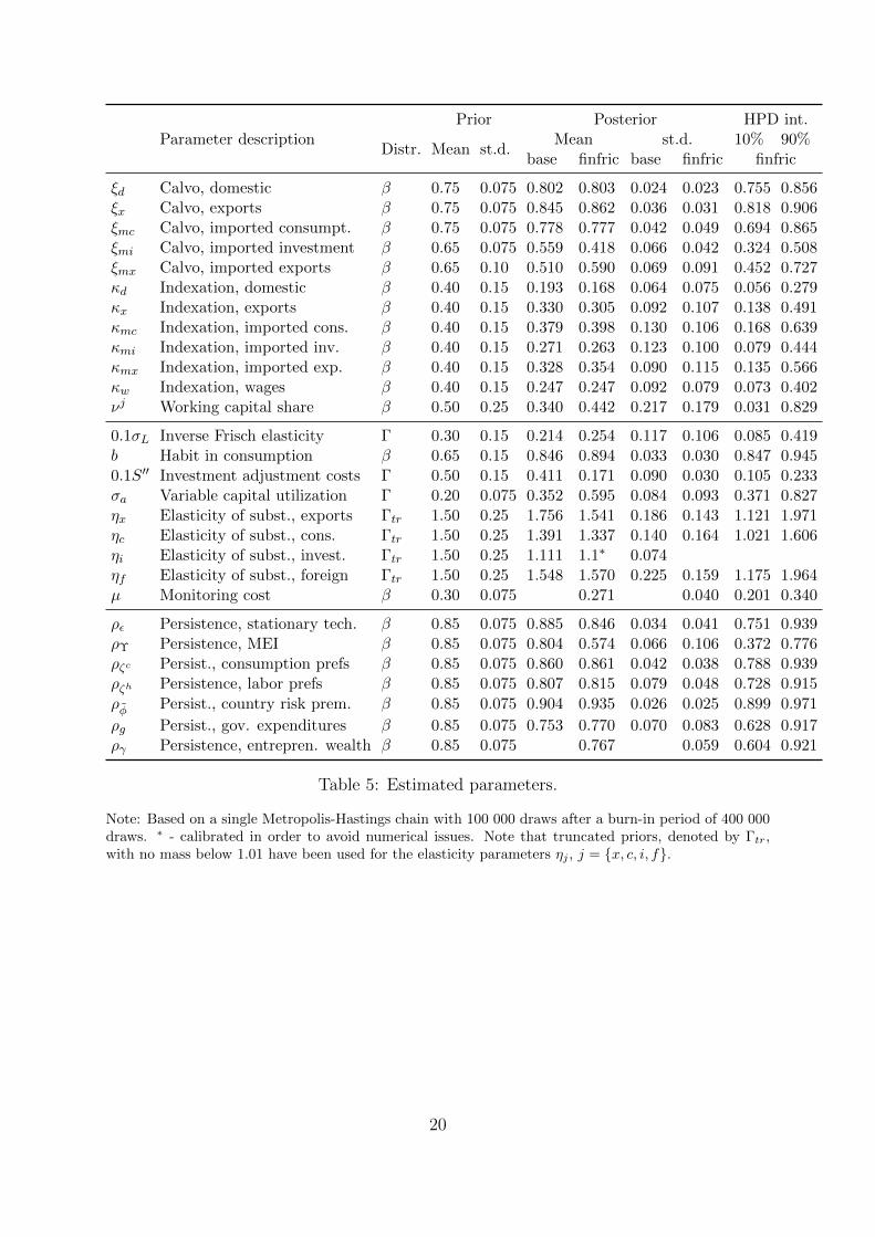
The posterior parameter estimates for the foreign block are reported in Tables 3 and 4, andthose specific to the domestic block - in Tables 5 and 6. The priors were deliberately fixedto be the same across the two models for a more transparent comparison, and favor thebaseline model. The estimated mode of the elasticity of substitution of investment goodsparameter, ηi, is close to unity and thus the parameter is calibrated for the financialfrictions model to 1.1, similar to the posterior mean in the baseline model, in orderto avoid numerical issues. Overall, the estimated posterior means of the parametersare similar between the two models. The most notable difference is in the investmentadjustment costs parameter which is about 2.4 times lower for the financial frictionsmodel compared to the baseline specification. They are statistically significantly differentat 10% significance level. The lower parameter indicates that the financial frictions modelinduces the gradual response that the investment adjustment mechanism was introducedto generate. Also, the estimated persistence parameter of the marginal efficiency ofinvestment (henceforth MEI) shock is reduced (from 0.80 to 0.57) with the introductionof the financial frictions block. Regarding the estimated standard deviations of shocks, thefinancial frictions model assigns a smaller standard deviation to the marginal efficiencyof investment shock, which, apparently, is ‘crowded out’ by the entrepreneurial wealthshock.

Tables 3 - 6 about here

7

4.2 Model moments and variance decomposition

4.2.1 Model moments

Table 7 presents the data and the model means and standard deviations for the ob-served time series. The table shows that there is a substantial variation of growth ratesin the data, especially between the domestic and foreign variables, which is why realquantities, the domestic inflation rates and the real exchange rate are demeaned beforematching the model to the data. The standard deviations are matched rather well buttheir over-estimation is evident for total hours, GDP, imports, as well as for the interestrate spread10. The introduction of the financial frictions block appears to slightly lessenthis over-estimation issue.

Table 7 about here

4.2.2 Conditional variance decomposition

The conditional variance decomposition at eight quarters forecast horizon is reportedin Table 8. (Those at one, four and twenty quarters forecast horizons are reported inAppendix B.).

Table 8 about here

Entrepreneurial wealth shock versus marginal efficiency of investment shockTable 8 shows that the entrepreneurial wealth shock, which is specific to the financialfrictions model and absent from the baseline model, ‘crowds out’ the marginal efficiencyof investment (MEI) shock by reducing its share of explaining the variance of investmentfrom 74% (baseline) to 28% (financial frictions model), the variance of net exports toGDP ratio from 60% to 6%, and the variance of GDP from 15% to 4%. As a reminder,MEI shock enters in the capital accumulation equation ((C.38) in Appendix) and affectshow (efficiently) investment is transformed into capital. This is the shock whose impor-tance is emphasized in Justiniano, Primiceri and Tambalotti (2011), where one of theirinterpretations of this shock being a proxy for the effectiveness with which the financialsector channels the flow of the household savings into a new productive capital.

The entrepreneurial wealth shock explains 10% of the variance of GDP, 45% of thevariance of investment, 35% of the net exports to GDP ratio, 51% of entrepreneurial networth and 69% of the spread between the nominal interest rate paid by the entrepreneurand the risk-free one.

CTW do not report the conditional variance decomposition for the baseline model,but with the financial frictions together with the search and matching frictions in labormarket (without additional shock added) which are absent in my financial frictions model.Also, their model is estimated for Swedish data with inflation-targeting monetary policy.Nevertheless, it is instructive to compare the results of CTW with ours. The results ofCTW suggest that, when financial frictions mechanism is present, MEI shock explains10% of the variance of investment, 7% of the variance of net exports to GDP ratio, and

10CTW note that their use of ‘endogenous prior’ reduces the effect of over-estimated shock standarddeviations. I’m not using such a prior.

8

4% of the variance of GDP. Also, the entrepreneurial wealth shock explains 71% of thevariance of investment, 23% of the variance of the net exports to GDP ratio, 25% ofthe variance of GDP, 64% of entrepreneurial net worth, and 60% of the variance of thespread. CTW briefly mention, but do not report in tables, the effect of shutting down thefinancial shock in their model. In that case, MEI shock becomes more important in thevariance decomposition: it explains 52% of the variance of investment and 6% of GDP.These results are broadly in line with mine except for the variance of investment whichappears to be better explained by the entrepreneurial wealth shock than by MEI shockin Sweden compared to Latvia. The difference is likely due to the milder response ofentrepreneurial net worth to the wealth shock in Latvia compared to Sweden, reflectingthe fact that Swedish financial markets are more developed.

Country risk premium shock Table 8 also reports that the country risk premiumshock is the major driving force of the domestic nominal interest rate and a crucial factorin Latvia’s business cycles. This is more so in the financial frictions model comparedto the baseline. So, for the given sample of 1995Q1-2012Q4, the country risk premiumshock explains 92% of the variance of the domestic nominal interest rate (versus 87% inbaseline), 11% of the variance of investment (versus 5% in baseline), 3% of the varianceof GDP (versus 1% in baseline), 18% of the variance of net exports to GDP ratio (versus10% in baseline) and 13% of the variance of the entrepreneurial net worth.

Comparing to the results of CTW, there are big differences. For Sweden, this shockexplains only 5% of the variance of nominal interest rate, 1% of the variance of investment,and 1% of the variance of net worth, while the variance of GDP is explained by aboutthe same amount as in Latvia, i.e. 3%. The reason for the difference is that, during thespecific historic sample, the domestic nominal interest rate in Latvia has been higher thanthan in the euro area and given that, in the model, Latvia’s currency is hard-pegged tothe euro, the (huge historic) difference between the actual domestic and foreign interestrates is explained by the country risk premium. It is expected that, since Latvia’s joiningthe euro area in 2014, the weight of the country risk premium shock on the domesticinterest rate will diminish, giving more influence to the euro area-wide shocks.

Shocks in the foreign economy block The effect of the foreign interest rate, foreignoutput and foreign inflation shocks on the domestic economy is estimated to be ratherlimited, with the greatest influence being to the domestic nominal interest rate. The unit-root technology shock also has been estimated to have little influence on the domesticeconomy during the particular historic period.

These results are broadly close to the results of CTW who also find negligible role ofthe shock to foreign interest rate, foreign output and foreign inflation to Swedish econ-omy. Though, their estimated effect of the unit-root technology shock is more influential,explaining 4.1% of the variance of Swedish GDP compared to 0.1% for Latvia’s GDP. Thelatter result might be explained by the fact that, during the particular historic episode,Latvia’s economy has been on its more or less idiosyncratic catching-up boom-bust cy-cle, while the more developed Swedish economy has been more reliant on the world-widetechnology growth. Also, CTW estimate this shock based on the trade-weighted foreignvariables, while I use the euro area variables, thus the link (the common technology)between the domestic and foreign variables is looser in my case.

9

Stationary neutral technology shock While touching upon technology shocks, an-other difference between CTW results for Sweden and mine for Latvia is in the effect ofthe stationary neutral technology shock affecting the intermediate goods producers’ pro-duction function. This shock is estimated to have minor influence on Latvia’s economyexcept for total hours worked (11% of the variance explained by this shock).

CTW estimation shows that this shock explains about the same portion of the varianceof hours worked (9%) but also 11% of the variance of consumption (0.1% for Latvia), 9%of the variance of GDP (0.8% for Latvia), 6% of CPI inflation (1% for Latvia) and 8% ofthe domestic nominal interest rate (0.0% for Latvia). Apparently, other domestic shockshave compensated the lack of influence of the stationary technology shock on Latvia’seconomy.

Household preference shocks Noticeable, The consumption preference shock ex-plains 82% of the variation of consumption in Latvia, whereas ‘only’ 45% in Sweden.This difference might be explained by the strong consumption-driven boom that Latviaexperienced starting around 2004 (see the historic shock decomposition below).

The labor preference shock is estimated to have about the same effect on both countriesat least with respect to wages; this shock is estimated to explain 39% of the variance ofreal wages in both Latvia and Sweden. The effects on other labor market variables differ,but this is, most probably, due to the different structure of labor market modeling blockin the models.

Domestic markup shock The domestic markup shock, affecting marginal cost ofproducing the domestic intermediate good, is estimated to explain 27% of Latvia’s CPIinflation (45% in Sweden) and 39% of the variance in real wage (31% in Sweden). Thiscompletes the similarities of this shock across the countries, since, given Latvia’s pegregime, this shock explains 23% of the variance of Latvia’s real exchange rate (0.2% inSweden), while in Sweden, it affects, through Taylor rule, the nominal interest rate, andparts of real economy stronger than in Latvia; e.g. it explains 7% of the variance ofSwedish GDP and 3% of the variance of Swedish investment, while these figures are 2%and 0.1% for Latvia.

Export goods markup shock Table 8 shows that the markup shock on export goodsis estimated to have little effects on Latvia’s economy; the only noticeable ones are the2.5% (up from 1% in baseline) of the variance of GDP and 2% (up from 1% in baseline) ofthe variance of hours worked, while in Sweden these figures are 8% and 10%, respectively.Again, given the model differences, it is hard to point exact source of the discrepancy.A small part of the difference11 is due to the higher calibrated imported goods sharein exports for Latvia (55%) than for Sweden (35%), resulting in a smaller effect of theexports markup on Latvia’s GDP and hence hours worked, since the markup on importedexports is subject to a separate, imported exports markup shock.

Imported markup shocks The imported exports markup shock, indeed, has moreweight on Latvia’s economy than on Swedish: it is estimated to explain 35% of the

11I have checked this claim by recalibrating the model.

10

variance of Latvia’s GDP (16% for Sweden) and 30% of the variance of total hoursworked in Latvia (14% in Sweden).

Regarding the rest of the imported goods markup shocks, the imported consumptionmarkup shock explains the majority, 51% of the variance of the the domestic CPI inflation(up from 39% in baseline and 34% in Sweden), and hence is the major shock affecting thereal exchange rate (it explains 45% (up from 34% in baseline) of the variance of Latvia’sreal exchange rate, while in Sweden, this shock explains, through Taylor rule, 17% of thevariance of the nominal interest rate but less so the real exchange rate. In contrast to thedomestic markup shock, the imported consumption markup shock is estimated to have anon-negligible effect on Latvia’s GDP - it explains almost 4% (up from 1% in baseline) ofthe variance of Latvia’s GDP, while only 0.2% of Swedish GDP. The importance of thiseffect, again, can be explained by the strong consumption-driven boom Latvia’s economyexperienced during the considered sample span.

Finally, the imported investment markup shock explains 7% (down from 10% in base-line) of the variance of investment, 18% (down from 30% in baseline) of the varianceof GDP, and 27% (down from 42.5% in baseline) of the variance of total hours worked.Quite differently, this shock is estimated to have negligible effect on Swedish economy.One explanation for the difference might be the higher calibrated imports share in in-vestment goods for Latvia (65%) than in Sweden (43%) but this must be only a partof the answer. Another eye-catching result is the large difference between the results offinancial frictions and baseline models. Absent of financial frictions block in the model,the imported investment markup shock would claim to explain almost a third of thevariance of Latvia’s GDP at two years forecast horizon, whereas it is less than one fifthwith the financial frictions block added to the model. The rest of the shock appears tobe attracted by consumption-related shocks - the consumption preference shock and theimported consumption markup shock.

Foreign shocks combined Overall, if the foreign shocks are defined as the three for-eign (interest rate, output, inflation) stationary shocks, the country risk premium shock,the world-wide unit root neutral technology shock, the markup shocks on imports (im-ported exports, consumption, investment) and exports - in total, 10 shocks - see thebottom row of Table 8, then they explain 99% of the variance in the domestic nominalinterest rate (up from 95% in the baseline and 28% in Sweden), the overwhelming partexplained by the country risk premium shock. Also, 53% and 62% of the variations ofCPI inflation and GDP, respectively, (versus 43% and 72% in baseline, and 40% and 32%in Sweden) at two year forecast horizon are explained by the foreign shocks, the over-whelming portion coming from markup shocks on imported consumption and domesticgoods (for CPI inflation) and on imported exports and imported investment (for GDP).

Since, in the literature, the sources of business cycles are largely related to fluctuationsin investment, the major source of the variance of investment in Latvia is estimated to bethe entrepreneurial wealth shock. Given the evidence from Sweden, the influence of thisshock is to be expected to grow as Latvia’s firms become more financially integrated.

11

4.3 Impulse response functions

Since Table 8 shows that the entrepreneurial wealth shock is the main driver of thevariance of investment in the financial frictions model and that it ‘crowds out’ MEI shockfrom the baseline model, it is instructive to compare the impulse response functions(henceforth IRF) of these two shocks.

Entrepreneurial wealth shock The IRF to the entrepreneurial wealth shock areplotted in Figure 1, which shows that a positive temporary entrepreneurial wealth shock,γt, drives up the net worth, reduces the expected bankruptcy rate and thus the interestrate spread, and increases the investment (by about the same percentage change as innet worth); GDP goes up accordingly, and so do the real wage and total hours worked.Both exports and imports increase but the latter increases more due to the demand forinvestment goods, thus net exports to GDP ratio decreases slightly. As a consequence,the net foreign assets to GDP ratio worsens, driving up a slight risk premium on thedomestic nominal interest rate. The shock causes the cost of investment to decrease, andconsumption to pick up only steadily. Therefore, CPI inflation decreases, though by asmall amount, and thus the real exchange rate depreciates.

The response of net worth to this and other shocks is quite muted, i.e. its dynamicsappear to die out in a few periods. This observation together with the autocorrelatedmeasurement error of net worth suggest that the stock market price index might be aweak proxy for net worth in Latvia, and thus other potential measures, such as the houseprice index, could be investigated. Such an option is left for future research.

Figure 1 about here

MEI shock Comparing the wealth shock to a temporary MEI shock, Figure 2 showsthat the effect of MEI shock in the baseline model is qualitatively similar to the effectof the wealth shock in the financial frictions model (except for the effect on consumptionwhich decreases initially), but the introduction of financial frictions dampens the effect ofMEI shock on all plotted variables (and consumption now slightly increases). The effectof these shocks on net worth and the spread is opposite; this is how the two shocks aredistinguished in the financial frictions model.

MEI shock increases the amount of capital per investment and thus the price ofcapital decreases. Consumption barely moves, thus MEI shock has a downward pressureon prices.

Figure 2 about here

Country risk premium shock Figure 3 shows the IRF to a temporary country riskpremium shock. As Table 8 shows, this shock is the major cause of the variance of thedomestic nominal interest rate. The effects are qualitatively similar across the modelsbut the financial frictions mechanism somewhat amplifies them. The shock increases thedomestic nominal interest rate which decays towards its steady state with persistence.This is followed by a decrease in consumption and entrepreneurial net worth, an increasein the spread and the bankruptcy rate (both reverse the sign after a year), and a decrease

12

in investment (initially, about twice as much with financial frictions mechanism com-pared to the baseline), GDP, real wage, and total hours worked. Imports decreases morethan exports, resulting in a slight increase in net exports to GDP ratio. CPI inflationdecreases for about two years, after which the sign is reversed. The real exchange ratethus depreciates for the first two years after the shock.

Figure 3 about here

Foreign nominal interest rate shock Table 8 shows that the foreign nominal inter-est rate shock has little influence on the domestic economy during the particular historicperiod; nevertheless, policy-makers are usually interested in what happens after an in-crease in the policy rate, and it is the European Central Bank’s policy rate that mattersfor Latvia after it joined the euro area in 2014. Figure 4 shows that a positive tempo-rary foreign nominal interest shock increases both the foreign and the domestic nominalinterest rate by the same amount, and both decay towards their steady state slowly. Con-sumption, investment and entrepreneurial net worth decrease, bankruptcy rate increasesmarginally (for the first year) and, as a result, so does the spread. GDP decreases, so doreal wage, and total hours worked. There is a negligible increase in net exports to GDPratio due to a decrease in imports. Thus, the net foreign assets to GDP ratio increasesslightly, fostering a decrease of the domestic country risk premium, and therefore, also ofthe domestic nominal interest rate. CPI inflation decreases due to the slower domesticactivity. The domestic inflation decreases by a larger amount than the foreign inflation,resulting in the initial but small depreciation of the real exchange rate. The effect issimilar across the models except for the more persistent dynamics of the nominal interestrate under the financial frictions mechanism.

The impulse response functions are similar between the country risk premium and theforeign nominal interest rate shocks, thus signaling the potential identification issues ofthese two shocks. The particular procedure of estimating the foreign BVAR separatelyfrom the domestic block mitigates the identification problem somewhat. The replacementof the foreign BVAR with a full-blown foreign DSGE block could be a cure since it wouldidentify the foreign monetary policy better but at the cost of model complexity.

The rest of the IRF are plotted in Appendix B.

Figure 4 about here

4.4 Smoothed shock values and historical decomposition

Figures 5 and 6 show the smoothed shock values for the financial frictions model. Thetable summarizing their means and standard deviations are relegated to Appendix B.These figures show that the means of the shocks are about zero. As to the downside, themeasurement errors of the net worth, total hours worked, and real wage appear to beautocorrelated.

Figures 5 and 6 about here

Figures 7 to 13 show the historic shock decomposition of GDP, CPI inflation and theinterest rate spread.

13

GDP Concentrating on the most sizable shocks, Figures 7 - 8 show that the modelidentifies the shock to household consumption preferences as the most important drivingforce of the 2004-boom. During the period of 2004-2007, the values of this shock werepersistently above the sample average (see Figure 5), signifying that households wereespecially keen on spending on consumption goods during that period. The shock ceasedduring the second half of 2007, probably due to the rising costs of living and thus thedecreasing consumer confidence (the latter is backed by the ECFIN consumer surveydata). At that time several other shocks became adverse, including the stationary andunit-root neutral technology shocks, and the risk premium shock (see Figure 5). Startingfrom 2008 and up to 2011, a series of negative entrepreneurial wealth shocks is identifiedto have significantly affected GDP growth (Figure 7). In fact, this shock has become themajor source determining the GDP level during the post-recession episode, see Figure 8.In the model, the dynamics of the entrepreneurial wealth is observable and measured bythe OMX Riga share price index, which plummeted during the recession. In practice, itis likely that the variable captures also a part of the dynamics in the real estate prices(otherwise, the real estate sector is not present in the model), which also fell sharplyduring the recession as a result of the burst of the housing bubble.

Figures 7 - 8 about here

For comparison, Figures 9 - 10 show the growth decomposition delivered by the base-line model (smoothed shock figures are skipped due to space constraints). The baselinemodel identifies MEI shock as one of the most important shocks driving the 2004-boomand the subsequent recession. According to the baseline model, MEI shock has con-tributed negatively over the whole post-recession period, which is not easy to interpret.


Therefore, having the financial frictions block in the model both clarifies and changesthe story. First, the entrepreneurial wealth shock behaves differently than MEI shock,since the former has played little role during the boom period. Thus, consumption pref-erences are left as the single most important factor creating the 2004-boom. Second, theentrepreneurial wealth shock is more easily understandable force that has deepened therecession but ceased to be active during the post-recession episode. On the contrary, inthe baseline model, the ever-active MEI shock during the post-recession period is harderto explicate.

CPI inflation Figure 11 shows that the model identifies the shock to household laborpreferences as the major driving force of Latvia’s CPI inflation up in the 2004-boom,coupled with the imported consumption markup shocks in 2007, and these same shockstogether with the domestic markup shocks drew CPI inflation down in 2009.

The labor preference shock determines the household willingness to work. The modelidentifies that, during the period of 2005-2007 households in Latvia were keen to workless (and to consume more), relative to the sample average (see Figure 7). The disutilityfrom work arose probably due to the rapidly growing economy and thus the relatively easymoney available for spending. Shirking drove wages up to compensate for the household

14

disutility from work; and that in turn, pushed the price of consumption goods up. Begin-ning from late 2008 and continuing until the sample ends in 2012Q4, the labor preferenceshock is identified to have downward pressure on CPI inflation, which could be explainedby the increased necessity to earn a living due to lower wages and fewer vacancies.

The markup shock to imported consumption goods raises the price of imported con-sumption goods. The model identifies that the level of this shock was persistently aboveits sample average during the year 2008, the time at which the consumption preferenceshock had already become flat or even negative, and coinciding with the period of theabove average foreign inflation shock (unaffected by the domestic block, since estimatedseparately) and the peak in both the crude oil and natural gas prices. It is likely that theimported consumption markup shock captures the increase in the cost of energy, sincethe price of energy is not present in the model but through foreign inflation. Apparently,the foreign inflation variable is not able to fully represent the dynamics of imported costs,thus the rest is absorbed by the markup shock. For example, the price of natural gasaffects the heating bills. It was a matter of fact that heating bills rose during the year2008, constituting up to three percentage points of the annual inflation at that time.Overall, the model suggests that the imported consumption markup shock constitutedabout a half of the annual CPI inflation during the year 2008.

The domestic markup shock affects the marginal cost of domestic production before itis affected by the foreign markup shocks. The model identifies a series of negative domesticmarkup shock during 2009 (probably due to the easing in labor market, the reforms inthe public sector, postponed investment projects or dividend payments by firms), andpartly rebalancing during late 2010-2011, which pushed CPI inflation upwards.

The presence of the financial frictions block in the model reduces slightly the role ofMEI shock and stationary technology shock on CPI inflation, see Figure 12.


Interest rate spread Figure 13 shows that the entrepreneurial wealth shock is themain driving force behind the interest rate spread. The increased spread in the 2008-recession is explained mainly by a negative temporary wealth shock. MEI shock has alsocontributed to affect the spread but its role has been different from the wealth shock:MEI shock’s contribution has been mild during the recession episode. Rather, it hascontributed to reduce the spread during the boom period (as the wealth shock but to agreater extent) and during the years 2011-2012 (counteracting the wealth shock). Again,as MEI shock is ad hoc, it is not easy to interpret it.

Figure 13 about here

4.5 Forecasting performance

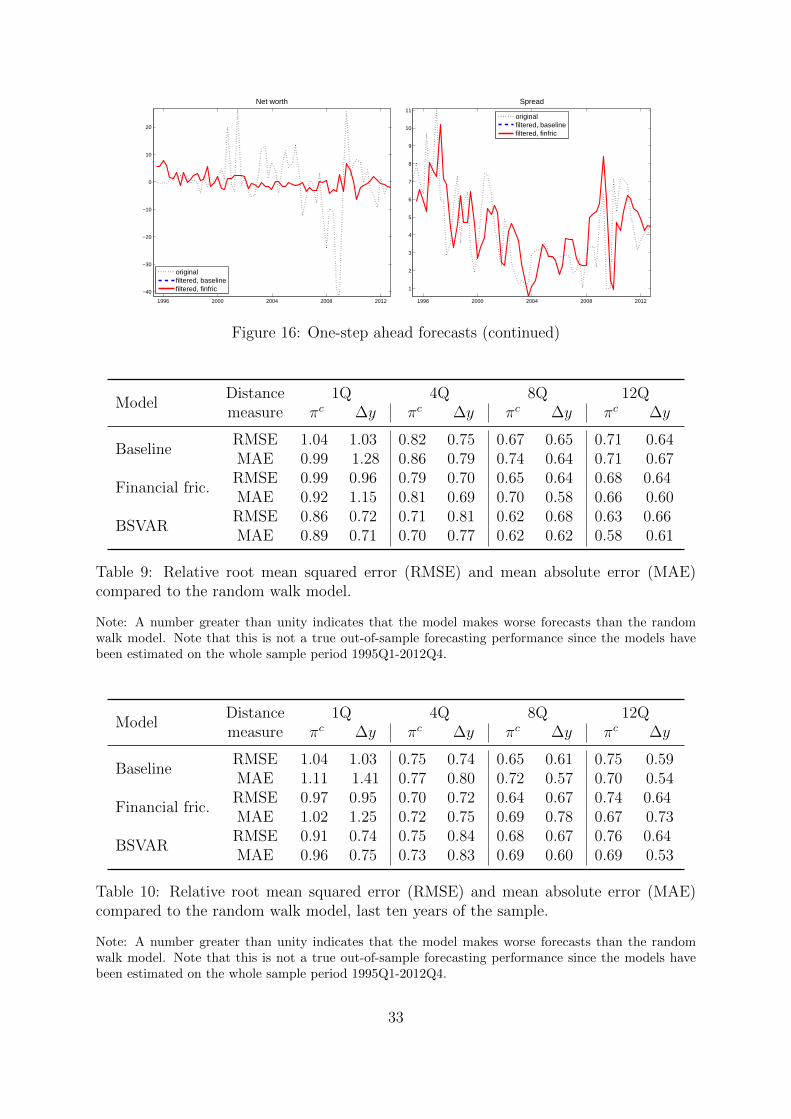
Figures 14 to 16 show one-step ahead forecasts of the baseline and the financial frictionsmodels for all the observables. These are not true out-of-sample forecasts because themodel is calibrated/estimated on the whole sample period 1995Q1-2012Q4. Nevertheless,these figures indicate approximate forecasting performance of the models. Particularly,it is informative to see whether the models tend to yield unbiased forecasts. The results

15

show that the models forecast relatively well. No crucial biases are evident, except forthe CPI inflation which appears to be slightly upward biased. The total hours workedforecasts are rather volatile, inducing this volatility in the GDP series. On the positiveside, the pick up of the interest rate spread in 2009 is forecasted in advance thus indicatingthat the model, potentially, could be applied in forecasting financial stress.

Figures 14 to 16 about here

Table 9 reports the forecasting performance of the baseline and financial frictionsmodels relative to a random walk model (in terms of quarterly growth rates) with respectto predicting CPI inflation and GDP for horizons: one, four, eight and 12 quarters. I alsoreport the forecasting performance of a BSVAR (with the same structure as the foreignBSVAR, and with similar priors), since it is often taken as a benchmark in the literature12.Table 9 shows that both models forecast both variables at least as precisely as the randomwalk model at all horizons considered. Both models outperform the random walk by about30% in forecasting both variables for horizons two to three years, and deliver about thesame precision at a one quarter horizon. Moreover, the financial frictions model tends todeliver somewhat more precise forecasts than the baseline model of both CPI inflationand GDP, and a comparable forecasting precision to that of a BSVAR.

Repeating the exercise for only the last ten years of the sample shows the financialfrictions model still performs roughly as well as the baseline and a BSVAR models (Table10). Thus, the model can be used not only for policy studies but also for forecastingpurposes. The results from our forecasting exercise are similar to those of CTW who alsofind that the financial frictions model tends to outperform slightly the baseline model.

Table 9 about here

5 Summary and conclusions

This paper builds a DSGE model for Latvia that would be suitable to replace the tradi-tional macro-econometric model currently employed as the main macroeconomic modelat Bank of Latvia. For that purpose, I adapt the Christiano, Trabandt and Walentin(2011, henceforth CTW) financial frictions model to Latvia’s data. The monetary policyis altered to become a nominal interest rate peg to the foreign interest rate. I study themodel fit, impulse response functions, conditional forecast variance decomposition, shockhistoric decomposition, and forecasting performance, and compare the outcome to thatof the model without the financial accelerator block (the ‘baseline’ model), as well as tothe findings of CTW.

The main findings are as follows. The addition of financial frictions block providesmore appealing interpretation for the drivers of economic activity, and allows to reinter-pret their role. Financial frictions played an important part in Latvia’s 2008-recession.The financial frictions model beats both the baseline model and the random walk modelin forecasting both CPI inflation and GDP, and performs roughly the same as a BSVAR.

12The particular BSVAR has some economically implausible estimated parameters, since Latvian GDP,CPI inflation and nominal interest rate data do not possess a stable and economically plausible relation-ship over the particular sample span.

16

Overall, the results suggest that the financial frictions model is suitable in both policyanalysis and forecasting exercises, and is an improvement over the model without thefinancial frictions block.

References

[1] Adjemian, Stephane, Bastani, Houtan, Juillard, Michel, Karame, Frederic, Mi-houbi, Ferhat, Perendia, George, Pfeifer, Johannes, Ratto, Marco and Villemot,Sebastien, 2011. “Dynare: Reference Manual, Version 4” Dynare Working Papers,1, CEPREMAP.

[2] Adolfson, Malin, Laseen, Stefan, Linde, Jesper and Villani, Mattias, 2008. “Evaluat-ing an estimated new Keynesian small open economy model”, Journal of EconomicDynamics and Control, vol. 32(8), 2690-2721.

[3] Bernanke, Ben, Mark Gertler and Gilchrist, Simon, 1999. “The financial acceleratorin a quantitative business cycle framework”, Handbook of Macroeconomics, editedby John B. Taylor and Michael Woodford, Elsevier Science, 1341-1393.

[4] Christiano, Lawrence J., Eichenbaum, Martin and Evans, Charles L., 2005. “NominalRigidities and the Dynamic Effects of a Shock to Monetary Policy”, Journal ofPolitical Economy, vol. 113(1), 1-45.

[5] Christiano, Lawrence J., Trabandt, Mathias and Walentin, Karl, 2011.“Introducingfinancial frictions and unemployment into a small open economy model” Journal ofEconomic Dynamics and Control, vol. 35(12), 1999-2041.

[6] Dixit, Avinash K. and Stiglitzh, Joseph E., 1977. “Monopolistic Competition andOptimum Product Diversity”, American Economic Review, vol. 67(3), 297-308.

[7] Erceg, Christopher J., Dale W. Henderson and Andrew T. Levin, 2000. “Optimalmonetary policy with staggered wage and price contracts”’, Journal of MonetaryEconomics, vol. 46(2),281-313.

[8] Fisher, Irving, 1933. “The debt-deflation theory of great depressions”, Econometrica,vol. 1(4), 337-357.

[9] Justiniano, Alejandro, Giorgio Primiceri and Andrea Tambalotti, 2011. “Investmentshocks and the relative price of investment”, Review of Economic Dynamics, vol.14(1), 101-121.

[10] Stehrer, Robert, 2013. “Accounting Relations in Bilateral Value Added Trade”, wiiwWorking Papers 101, The Vienna Institute for International Economic Studies, wiiw.

17

Appendix A Tables and Figures

Parameter Value Description

α 0.400 Capital share in productionβ 0.995 Discount factorωc 0.450 Import share in consumption goodsωi 0.650 Import share in investment goodsωx 0.550 Import share in export goods

φa 0.010 Elasticity of country risk to net asset positionηg 0.202 Government expenditure share of GDPτk 0.100 Capital tax rateτw 0.330 Payroll tax rateτc 0.180 Consumption tax rateτy 0.300 Labor income tax rateτb 0.000 Bond tax rateµz 1.005 Steady state growth rate of neutral technologyµψ 1 Steady state growth rate of investment technologyπ 1.005 Steady state inflation growth targetλw 1.500 Wage markupλd;m,c;m,i 1.300 Price markup for the domestic, imp. consump., imp. investm. goodsλx;m,x 1.200 Price markup for exports and imported exports goodsϑw 1.000 Wage indexation to real growth trendκj 1− κj Indexation to inflation target for j = d;x;m, c;m, i;m,x;wπ 1.005 Third indexing base

φS 0 Country risk adjustment coefficient

Financial frictions model

F (ω) 0.020 Steady state bankruptcy rate100We/y 0.100 Transfers to entrepreneurs

Table 1: Calibrated parameters.

Parameter descriptionPosterior mean

Moment Moment valuebaseline finfric

δ Depreciation rate of capital 0.030 0.030 pii/y 0.255ϕ Real exchange rate 2.16 2.02 SP xX/(PY ) 0.462AL Scaling of disutility of work 16.86 24.46 Lς 0.270γ Entrepreneurial survival rate 0.96 n/(pk′k) 0.600

Table 2: Matched moments and corresponding parameters.

Note: The quarterly depreciation rate of capital is fixed at three percent.

18

Parameter descriptionPrior Posterior HPD int.

Distr. Mean st.d. Mean st.d. 10% 90%

ρµz Persistence, unit-root tech. β 0.50 0.075 0.590 0.063 0.487 0.696a11 Foreign VAR parameter N 0.90 0.05 0.913 0.034 0.852 0.977a22 Foreign VAR parameter N 0.50 0.05 0.521 0.055 0.438 0.605a33 Foreign VAR parameter N 0.90 0.05 0.954 0.023 0.919 0.989a12 Foreign VAR parameter N -0.10 0.10 -0.165 0.091 -0.314 -0.016a13 Foreign VAR parameter N -0.10 0.10 -0.045 0.054 -0.124 0.037a21 Foreign VAR parameter N 0.10 0.10 0.181 0.043 0.097 0.260a23 Foreign VAR parameter N -0.10 0.10 -0.090 0.055 -0.183 -0.008a24 Foreign VAR parameter N 0.05 0.10 0.078 0.041 0.009 0.146a31 Foreign VAR parameter N 0.05 0.10 0.080 0.029 0.032 0.131a32 Foreign VAR parameter N -0.10 0.10 -0.095 0.058 -0.198 0.002a34 Foreign VAR parameter N 0.10 0.10 0.108 0.026 0.068 0.149c21 Foreign VAR parameter N 0.05 0.05 0.021 0.040 -0.048 0.088c31 Foreign VAR parameter N 0.10 0.05 0.145 0.031 0.094 0.196c32 Foreign VAR parameter N 0.40 0.05 0.374 0.053 0.286 0.459c24 Foreign VAR parameter N 0.05 0.05 0.065 0.046 -0.003 0.135c34 Foreign VAR parameter N 0.05 0.05 0.048 0.034 -0.002 0.101

Table 3: Estimated foreign SVAR parameters.

Note: Based on a single Metropolis-Hastings chain with 100 000 draws after a burn-in period of 900 000draws.

DescriptionPrior Posterior HPD int.

Distr. Mean st.d. Mean st.d. 10% 90%

100σµz Unit root technology Inv-Γ 0.25 inf 0.328 0.052 0.248 0.406100σy∗ Foreign GDP Inv-Γ 0.50 inf 0.317 0.055 0.219 0.4151000σπ∗ Foreign inflation Inv-Γ 0.50 inf 0.593 0.118 0.394 0.805100σR∗ Foreign interest rate Inv-Γ 0.075 inf 0.067 0.008 0.054 0.079

Table 4: Estimated standard deviations of SVAR shocks.


19

Parameter descriptionPrior Posterior HPD int.

Distr. Mean st.d.Mean st.d. 10% 90%

base finfric base finfric finfric

ξd Calvo, domestic β 0.75 0.075 0.802 0.803 0.024 0.023 0.755 0.856ξx Calvo, exports β 0.75 0.075 0.845 0.862 0.036 0.031 0.818 0.906ξmc Calvo, imported consumpt. β 0.75 0.075 0.778 0.777 0.042 0.049 0.694 0.865ξmi Calvo, imported investment β 0.65 0.075 0.559 0.418 0.066 0.042 0.324 0.508ξmx Calvo, imported exports β 0.65 0.10 0.510 0.590 0.069 0.091 0.452 0.727κd Indexation, domestic β 0.40 0.15 0.193 0.168 0.064 0.075 0.056 0.279κx Indexation, exports β 0.40 0.15 0.330 0.305 0.092 0.107 0.138 0.491κmc Indexation, imported cons. β 0.40 0.15 0.379 0.398 0.130 0.106 0.168 0.639κmi Indexation, imported inv. β 0.40 0.15 0.271 0.263 0.123 0.100 0.079 0.444κmx Indexation, imported exp. β 0.40 0.15 0.328 0.354 0.090 0.115 0.135 0.566κw Indexation, wages β 0.40 0.15 0.247 0.247 0.092 0.079 0.073 0.402νj Working capital share β 0.50 0.25 0.340 0.442 0.217 0.179 0.031 0.829

0.1σL Inverse Frisch elasticity Γ 0.30 0.15 0.214 0.254 0.117 0.106 0.085 0.419b Habit in consumption β 0.65 0.15 0.846 0.894 0.033 0.030 0.847 0.9450.1S′′ Investment adjustment costs Γ 0.50 0.15 0.411 0.171 0.090 0.030 0.105 0.233σa Variable capital utilization Γ 0.20 0.075 0.352 0.595 0.084 0.093 0.371 0.827ηx Elasticity of subst., exports Γtr 1.50 0.25 1.756 1.541 0.186 0.143 1.121 1.971ηc Elasticity of subst., cons. Γtr 1.50 0.25 1.391 1.337 0.140 0.164 1.021 1.606ηi Elasticity of subst., invest. Γtr 1.50 0.25 1.111 1.1∗ 0.074ηf Elasticity of subst., foreign Γtr 1.50 0.25 1.548 1.570 0.225 0.159 1.175 1.964µ Monitoring cost β 0.30 0.075 0.271 0.040 0.201 0.340

ρε Persistence, stationary tech. β 0.85 0.075 0.885 0.846 0.034 0.041 0.751 0.939ρΥ Persistence, MEI β 0.85 0.075 0.804 0.574 0.066 0.106 0.372 0.776ρζc Persist., consumption prefs β 0.85 0.075 0.860 0.861 0.042 0.038 0.788 0.939ρζh Persistence, labor prefs β 0.85 0.075 0.807 0.815 0.079 0.048 0.728 0.915

ρφ Persist., country risk prem. β 0.85 0.075 0.904 0.935 0.026 0.025 0.899 0.971

ρg Persist., gov. expenditures β 0.85 0.075 0.753 0.770 0.070 0.083 0.628 0.917ργ Persistence, entrepren. wealth β 0.85 0.075 0.767 0.059 0.604 0.921

Table 5: Estimated parameters.

Note: Based on a single Metropolis-Hastings chain with 100 000 draws after a burn-in period of 400 000draws. ∗ - calibrated in order to avoid numerical issues. Note that truncated priors, denoted by Γtr,with no mass below 1.01 have been used for the elasticity parameters ηj , j = {x, c, i, f}.

20

DescriptionPrior Posterior HPD int.

Distr. Mean st.d.Mean st.d. 10% 90%

base finfric base finfric finfric

10σε Stationary technology Inv-Γ 0.15 inf 0.139 0.126 0.016 0.014 0.103 0.149σΥ Marginal efficiency of invest. Inv-Γ 0.15 inf 0.234 0.162 0.056 0.027 0.093 0.230σζc Consumption prefs Inv-Γ 0.15 inf 0.143 0.227 0.029 0.056 0.131 0.320σζh Labor prefs Inv-Γ 0.50 inf 0.739 0.804 0.430 0.283 0.300 1.293

100σφ Country risk premium Inv-Γ 0.50 inf 0.547 0.554 0.044 0.045 0.475 0.632

10σg Government expenditures Inv-Γ 0.50 inf 0.468 0.470 0.044 0.041 0.396 0.544στd Markup, domestic Inv-Γ 0.50 inf 0.383 0.374 0.105 0.089 0.179 0.555στx Markup, exports Inv-Γ 0.50 inf 0.813 1.004 0.298 0.391 0.439 1.556στm,c Markup, imports for cons. Inv-Γ 0.50 inf 0.887 0.812 0.463 0.329 0.278 1.421στm,i Markup, imports for invest. Inv-Γ 0.50 inf 0.895 0.458 0.340 0.078 0.282 0.620στm,x Markup, imports for exports Inv-Γ 0.50 inf 1.052 1.447 0.410 0.643 0.523 2.34910σγ Entrepreneurial wealth Inv-Γ 0.50 inf 0.307 0.042 0.231 0.384

Table 6: Estimated standard deviations of shocks.


Variable ExplanationMean Standard deviation

DataModel

DataModel

baseline finfric baseline finfric

π Domestic inflation 6.08 2.00 2.00 8.39 8.82 8.61πc CPI inflation 5.62 2.00 2.00 6.29 8.80 8.51πi Investment inflation 6.78 2.00 2.00 51.45 49.57 46.49R Nom. interest rate 7.06 6.04 6.04 5.86 5.67 6.40∆h Total hours growth 0.02 0.00 0.00 2.20 6.76 5.69∆y GDP growth 1.37 0.50 0.50 2.31 5.37 4.56∆w Real wage growth 1.06 0.50 0.50 2.35 2.97 2.89∆c Consumption growth 1.47 0.50 0.50 2.84 3.16 3.39∆i Investment growth 1.73 0.50 0.50 16.32 21.34 21.65∆q Real exch. rate growth -0.88 0.00 0.00 2.51 2.29 2.22∆g Gov. expendit. growth 0.44 0.50 0.50 5.46 5.30 5.30∆x Export growth 2.19 0.50 0.50 3.41 3.67 3.66∆m Import growth 2.22 0.50 0.50 6.30 12.24 9.76∆n Stock market growth 1.32 0.50 10.38 14.92spread Interest rate spread 4.29 3.01 2.25 5.48∆y∗ Foreign GDP growth 0.26 0.50 0.50 0.61 0.52 0.52π∗ Foreign inflation 2.01 2.00 2.00 0.72 0.88 0.88R∗ Foreign nom. int. rate 3.16 6.04 6.04 1.61 2.58 2.58

Table 7: Data and (first-order approximated) model moments (in percent).

Note: The inflation and interest rates are annualized.

21

Description model R πc GDP C I NXGDP H w q N Spread

εtStationarytechnology

B 0.0 1.8 0.9 0.4 0.1 0.1 6.1 1.0 1.5F 0.0 1.2 0.8 0.1 0.0 0.5 10.9 0.7 1.0 0.2 0.1

Υt MEIB 5.1 1.2 15.1 1.7 73.6 60.2 6.9 1.5 1.0F 0.1 0.1 3.8 0.1 28.5 5.7 5.4 0.5 0.1 19.0 19.2

ζctConsumptionprefs

B 0.1 0.1 2.0 78.4 0.5 2.1 1.6 0.1 0.1F 0.3 0.3 8.7 81.6 0.2 19.1 6.9 0.2 0.2 0.2 0.1

ζht Labor prefsB 0.0 12.0 3.9 3.0 0.8 0.4 4.1 45.3 10.4F 0.1 8.7 3.1 1.9 0.6 3.5 4.3 39.1 7.5 1.3 0.4

τdtMarkup,domestic

B 0.0 32.0 1.2 0.2 0.1 0.1 0.8 37.7 27.5F 0.0 26.6 1.8 0.1 0.1 0.2 1.5 39.2 22.9 0.6 0.1

τxtMarkup,exports

B 0.0 0.0 1.2 0.0 0.0 0.0 1.0 0.0 0.0F 0.0 0.0 2.5 0.0 0.0 0.1 2.1 0.0 0.0 0.0 0.0

τmctMarkup, imp.for cons.

B 0.0 39.0 1.1 0.1 0.0 0.3 0.9 1.4 34.3F 0.0 50.8 3.8 0.0 0.0 0.9 3.1 2.5 44.7 0.1 0.0

τmitMarkup, imp.for inv.

B 1.1 3.0 29.6 0.2 9.6 14.6 42.5 0.7 2.5F 0.1 0.6 17.9 0.0 6.6 5.6 26.6 0.3 0.5 7.1 6.0

τmxtMarkup, imp.for exp.

B 0.3 0.1 38.9 0.1 0.1 6.8 32.2 0.3 0.1F 0.1 0.1 35.2 0.1 0.1 7.1 29.9 0.2 0.1 0.2 0.1

γtEntrepreneurialwealth

BF 0.8 1.0 10.4 0.2 44.8 35.1 1.9 1.1 0.9 51.5 69.2

φtCountry riskpremium

B 86.7 0.3 1.2 2.4 5.1 10.5 0.7 1.3 0.2F 92.0 0.7 2.7 3.9 11.1 17.8 1.1 3.6 0.6 13.5 2.2

µz,tUnit-roottechnology

B 1.6 0.1 0.1 0.1 0.2 1.4 0.0 0.4 0.3F 1.6 0.1 0.2 0.0 0.2 1.4 0.0 0.4 0.3 0.1 0.0

εR∗,tForeigninterest rate

B 1.6 0.1 0.1 0.2 0.3 0.9 0.0 0.1 0.0F 1.5 0.1 0.1 0.2 0.3 0.8 0.0 0.2 0.0 0.3 0.1

εy∗,t Foreign outputB 3.4 0.2 0.1 0.4 0.7 2.5 0.0 0.2 0.3F 3.4 0.1 0.0 0.6 0.3 2.1 0.0 0.3 0.5 0.1 0.1

επ∗,tForeigninflation

B 0.1 0.0 0.0 0.0 0.0 0.0 0.0 0.0 0.1F 0.1 0.0 0.0 0.0 0.0 0.0 0.0 0.0 0.1 0.0 0.0

5 foreign*B 93.3 0.7 1.4 3.1 6.4 15.3 0.8 2.0 1.0F 98.6 1.1 3.0 4.7 11.9 22.0 1.1 4.4 1.5 14.0 2.4

All foreign**B 94.8 42.8 72.3 3.5 16.1 37.0 77.3 4.5 38.0F 98.7 52.6 62.5 4.8 18.7 35.8 62.8 7.5 46.9 21.4 8.5

Table 8: Conditional variance decomposition (percent) given model parameter uncer-tainty at 8 quarters forecast horizon; posterior mean.

Note: ∗ ‘5 foreign’ is the sum of the foreign stationary shocks, R∗t , π∗t , Y ∗t , the country risk premium

shock, φt, and the world-wide unit root neutral technology shock, µz,t.∗∗ ‘All foreign’ includes the above five shocks as well as the markup shocks on imports and exports, i.e.τmct , τmit , τmxt and τxt . ‘B’ - baseline model, ‘F’ - financial frictions model.

22

Entrepreneurial wealth shock

baseline model financial frictions model foreign5 10 15 20

−0.15−0.1

−0.05

Net foreign assets/GDP (Lev.dev.)

5 10 15 20

−1.5−1

−0.5

Spread (ABP)

5 10 15 200

5

10

Net worth (% dev.)5 10 15 20

00.020.040.06

Real exch. rate (% dev.)

5 10 15 20

0.020.040.060.08

Real wage (% dev.)

5 10 15 20

00.20.4

Total hours (% dev.)5 10 15 20

−20−10

0

x 10−3Net exports/Y (Lev. dev.)

5 10 15 20

0

5

10Investment (% dev.)

5 10 15 200

0.020.04

Consumption (% dev.)5 10 15 20

00.20.40.6

GDP (% dev.)

5 10 15 20

−0.2−0.1

0

CPI inflation (ABP)

5 10 15 200

0.10.2

Nom. interest rate (ABP)

Figure 1: Impulse responses to the entrepreneurial wealth shock, γt.

Note: The units on the y-axis are either in terms of percentage deviation (% dev.) from the steady state,annualized basis points (ABP), or level deviation (Lev. dev.).

Marginal efficiency of investment shock


−0.3−0.2−0.1

0Net foreign assets/GDP (Lev.dev.)

5 10 15 200

0.20.40.60.8

Spread (ABP)

5 10 15 20

−4−2

0

Net worth (% dev.)5 10 15 20

00.020.040.060.08


5 10 15 200

0.050.1

Real wage (% dev.)

5 10 15 20

00.5

11.5


−0.04−0.02

00.02

Net exports/Y (Lev. dev.)

5 10 15 20

05

10

Investment (% dev.)

5 10 15 20−0.2−0.1

00.1


00.5

1

GDP (% dev.)

5 10 15 20−0.3−0.2−0.1

0

CPI inflation (ABP)

5 10 15 200

0.20.40.6


Figure 2: Impulse responses to the marginal efficiency of investment shock, Υt.


23

Country risk premium shock


0.020.040.060.080.10.120.14Net foreign assets/GDP (Lev.dev.)

5 10 15 20−0.2

00.20.4

Spread (ABP)

5 10 15 20−4−2

0

Net worth (% dev.)5 10 15 20

−0.020

0.020.04


5 10 15 20

−0.2−0.1

0

Real wage (% dev.)

5 10 15 20−0.4−0.2

0


05

1015


5 10 15 20

−4−2

0

Investment (% dev.)

5 10 15 20−0.3−0.2−0.1

0


−0.4

−0.20

GDP (% dev.)

5 10 15 20−0.2−0.1

00.1

CPI inflation (ABP)

5 10 15 20

0.51

1.52


Figure 3: Impulse responses to the country risk premium shock, φt.


Foreign nominal interest rate shock


0.010.020.030.040.05


5 10 15 20−0.05

0

0.05

Spread (ABP)

5 10 15 20−0.6−0.4−0.2

0

Net worth (% dev.)5 10 15 20

−505

1015

x 10−3Real exch. rate (% dev.)

5 10 15 20

−0.04−0.02

0

Real wage (% dev.)

5 10 15 20−0.08−0.06−0.04−0.02

00.02


2

4x 10

−3Net exports/Y (Lev. dev.)

5 10 15 20−0.8−0.6−0.4−0.2

0

Investment (% dev.)

5 10 15 20−0.08−0.06−0.04−0.02

0


−0.06−0.04−0.02

0

GDP (% dev.)

5 10 15 20−0.08−0.06−0.04−0.02

0CPI inflation (ABP)

5 10 15 200.05

0.10.15

0.20.25


Figure 4: Impulse responses to the foreign nominal interest rate shock, εR∗,t.


24

1996 2000 2004 2008 2012

−1

−0.5

0

unit−root technology

1996 2000 2004 2008 2012

−0.2

0

0.2

stationary technology

1996 2000 2004 2008 2012

−0.2

0

0.2

0.4marginal efficiency of inv.

1996 2000 2004 2008 2012

−0.6

−0.4

−0.2

0

0.2

0.4consumption preference

1996 2000 2004 2008 2012

−0.1

0

0.1foreign interest rate

1996 2000 2004 2008 2012

−1

0

1

country risk premium

1996 2000 2004 2008 2012

−1

0

1

labor preference

1996 2000 2004 2008 2012

−1

−0.5

0

0.5

foreign output

1996 2000 2004 2008 2012−1

−0.5

0

0.5

1

foreign inflation

1996 2000 2004 2008 2012

−1

0

1

government expenditure

1996 2000 2004 2008 2012

−1

−0.5

0

0.5

1

domestic markup

1996 2000 2004 2008 2012

−1

0

1

2

3

export markup

1996 2000 2004 2008 2012

−1

0

1

import consumption markup

1996 2000 2004 2008 2012−1

−0.5

0

0.5

1

import investment markup

1996 2000 2004 2008 2012

−2

0

2

import export markup

1996 2000 2004 2008 2012

−5

0

5

meas. GDP deflator

1996 2000 2004 2008 2012

−0.5

0

0.5

meas. real wage

1996 2000 2004 2008 2012

−1

−0.5

0

0.5

1

meas. consumption

Figure 5: Smoothed shock processes and measurement errors of the financial frictionsmodel.

25

1996 2000 2004 2008 2012−10

0

10

meas. investment

1996 2000 2004 2008 2012

−2

0

2

4meas. real x−rate

1996 2000 2004 2008 2012−0.5

0

0.5

meas. hours

1996 2000 2004 2008 2012

−1

−0.5

0

0.5

1

meas. output

1996 2000 2004 2008 2012

−1

0

1

meas. exports

1996 2000 2004 2008 2012−4

−2

0

2

4

meas. imports

1996 2000 2004 2008 2012

−4

−2

0

2

4

meas. CPI

1996 2000 2004 2008 2012

−20

0

20

meas. investment price

1996 2000 2004 2008 2012

−2

−1

0

1

2

meas. gov. expend.

1996 2000 2004 2008 2012

−0.5

0

0.5

entrepreneurial wealth

1996 2000 2004 2008 2012

−10

0

10

meas. net worth

1996 2000 2004 2008 2012

−2

−1

0

1

2

meas. spread

Figure 6: Smoothed shock processes and measurement errors of the financial frictionsmodel (continued).

26

2004 2008 2012−8

−6

−4

−2

0

2

4

consumption preference

labor preference

import inv. markup



Figure 7: Decomposition of GDP (quarterly growth rates), 2004Q1-2012Q4.

Note: Financial frictions model. Only those shocks that are greater than 2pp in at least one period.

2004 2008 2012

−20

−15

−10

−5

0

5

10

15

20



labor preference



initial values

Figure 8: Decomposition of GDP (levels), 2004Q1-2012Q4.

Note: Financial frictions model. Only those shocks that are greater than 4pp in at least one period.

27

2004 2008 2012

−6

−4

−2

0

2

4

6

marginal efficiency of inv.


labor preference

import inv. markup


Figure 9: Decomposition of GDP (quarterly growth rates), 2004Q1-2012Q4. Baselinemodel. Only those shocks that are greater than 2.5pp in at least one period.

2004 2008 2012

−15

−10

−5

0

5

10

15

20

25



foreign interest rate

labor preference

import inv. markup

Figure 10: Decomposition of GDP (levels), 2004Q1-2012Q4. Baseline model. Only thoseshocks that are greater than 4.5pp in at least one period.

28

2004 2008 2012

−15

−10

−5

0

5

10

15



labor preference

domestic markup

import cons. markup

meas. pic

Figure 11: Decomposition of CPI, 2004Q1-2012Q4.

Note: Financial frictions model. Only those shocks that are greater than 1.5pp in at least one period.

2004 2008 2012

−15

−10

−5

0

5

10

15



labor preference

domestic markup

import cons. markup

meas. pic

Figure 12: Decomposition of CPI, 2004Q1-2012Q4. Baseline model. Only those shocksthat are greater than 1.5pp in at least one period.

29

2004 2008 2012

−4

−2

0

2

4

6

8




labor preference

import inv. markup


meas. spread

Figure 13: Decomposition of interest rate spread, 2004Q1-2012Q4.

Note: Financial frictions model. Only those shocks that are greater than 0.8pp in at least one period.

30

1996 2000 2004 2008 2012

−10

−8

−6

−4

−2

0

2

4

Output

originalfiltered, baselinefiltered, finfric

1996 2000 2004 2008 2012

−30

−20

−10

0

10

20

Output price inflation


1996 2000 2004 2008 2012

5

10

15

20

25

Interest rate


1996 2000 2004 2008 2012

−6

−4

−2

0

2

4

6

Real wage


1996 2000 2004 2008 2012−14

−12

−10

−8

−6

−4

−2

0

2

4

Consumption


1996 2000 2004 2008 2012

−40

−30

−20

−10

0

10

20

30

Investment


1996 2000 2004 2008 2012

−20

−15

−10

−5

0

5

10

15

Government expenditure


1996 2000 2004 2008 2012

1

2

3

4

5

6

7

Foreign interest rate


Figure 14: One-step ahead forecasts

31

1996 2000 2004 2008 2012

−5

−4

−3

−2

−1

0

1

2

3

4

5

Real exchange rate


1996 2000 2004 2008 2012

−12

−10

−8

−6

−4

−2

0

2

4

Total hours


1996 2000 2004 2008 2012−16

−14

−12

−10

−8

−6

−4

−2

0

2

4

Exports


1996 2000 2004 2008 2012

−25

−20

−15

−10

−5

0

5

10

15

Imports


1996 2000 2004 2008 2012

−10

−5

0

5

10

15

20

CPI inflation


1996 2000 2004 2008 2012

−100

−50

0

50

100

Investment price inflation


1996 2000 2004 2008 2012

0

0.5

1

1.5

2

2.5

3

3.5

Foreign inflation


1996 2000 2004 2008 2012

−3

−2.5

−2

−1.5

−1

−0.5

0

0.5

Foreign output


Figure 15: One-step ahead forecasts (continued)

32

1996 2000 2004 2008 2012

−40

−30

−20

−10

0

10

20

Net worth


1996 2000 2004 2008 2012

1

2

3

4

5

6

7

8

9

10

11

Spread


Figure 16: One-step ahead forecasts (continued)

ModelDistance 1Q 4Q 8Q 12Qmeasure πc ∆y πc ∆y πc ∆y πc ∆y

BaselineRMSE 1.04 1.03 0.82 0.75 0.67 0.65 0.71 0.64MAE 0.99 1.28 0.86 0.79 0.74 0.64 0.71 0.67

Financial fric.RMSE 0.99 0.96 0.79 0.70 0.65 0.64 0.68 0.64MAE 0.92 1.15 0.81 0.69 0.70 0.58 0.66 0.60

BSVARRMSE 0.86 0.72 0.71 0.81 0.62 0.68 0.63 0.66MAE 0.89 0.71 0.70 0.77 0.62 0.62 0.58 0.61

Table 9: Relative root mean squared error (RMSE) and mean absolute error (MAE)compared to the random walk model.

Note: A number greater than unity indicates that the model makes worse forecasts than the randomwalk model. Note that this is not a true out-of-sample forecasting performance since the models havebeen estimated on the whole sample period 1995Q1-2012Q4.

ModelDistance 1Q 4Q 8Q 12Qmeasure πc ∆y πc ∆y πc ∆y πc ∆y

BaselineRMSE 1.04 1.03 0.75 0.74 0.65 0.61 0.75 0.59MAE 1.11 1.41 0.77 0.80 0.72 0.57 0.70 0.54

Financial fric.RMSE 0.97 0.95 0.70 0.72 0.64 0.67 0.74 0.64MAE 1.02 1.25 0.72 0.75 0.69 0.78 0.67 0.73

BSVARRMSE 0.91 0.74 0.75 0.84 0.68 0.67 0.76 0.64MAE 0.96 0.75 0.73 0.83 0.69 0.60 0.69 0.53

Table 10: Relative root mean squared error (RMSE) and mean absolute error (MAE)compared to the random walk model, last ten years of the sample.

Note: A number greater than unity indicates that the model makes worse forecasts than the randomwalk model. Note that this is not a true out-of-sample forecasting performance since the models havebeen estimated on the whole sample period 1995Q1-2012Q4.

33

Appendix B Computational appendix - not for pub-

lication



B 0.0 0.9 1.2 0.2 0.0 0.3 7.2 0.5 0.8F 0.0 0.7 1.1 0.1 0.0 0.8 13.1 0.4 0.6 0.1 0.1

Υt MEIB 0.0 0.0 9.0 1.3 70.0 23.3 6.4 0.4 0.0F 0.0 0.0 3.7 0.0 32.1 12.0 5.7 0.2 0.0 18.2 17.4


B 0.0 0.0 1.9 72.8 0.1 0.7 1.4 0.0 0.0F 0.0 0.1 6.9 75.1 0.2 4.2 5.1 0.2 0.1 0.2 0.1


τdtMarkup,domestic

B 0.0 36.8 1.6 0.2 0.1 0.4 1.0 44.0 30.5F 0.0 29.7 2.4 0.1 0.1 0.8 1.8 46.0 24.8 0.6 0.0

τxtMarkup,exports

B 0.0 0.0 1.6 0.0 0.0 0.1 1.1 0.0 0.0F 0.0 0.0 3.2 0.0 0.0 0.3 2.5 0.0 0.0 0.0 0.0


B 0.0 42.7 1.4 0.1 0.0 0.8 1.0 0.0 36.3F 0.0 53.8 4.6 0.0 0.0 2.6 3.4 0.0 46.1 0.1 0.0


B 0.1 2.4 29.0 0.1 10.6 41.7 41.8 0.6 2.0F 0.0 0.5 16.9 0.0 6.7 29.0 24.3 0.3 0.4 6.9 7.1


B 0.1 0.1 44.8 0.1 0.1 29.8 33.2 0.3 0.1F 0.0 0.1 39.8 0.0 0.1 30.9 31.7 0.2 0.1 0.2 0.2


BF 0.0 0.0 5.4 0.1 37.7 11.9 1.5 0.2 0.0 53.2 52.3


B 97.5 0.1 0.9 2.3 4.1 1.9 0.6 0.9 0.1F 97.6 0.2 2.4 3.0 10.5 5.1 0.6 2.2 0.2 12.9 5.8


B 0.1 0.0 0.1 0.0 0.2 0.3 0.0 0.1 0.1F 0.1 0.0 0.2 0.0 0.1 0.4 0.0 0.1 0.1 0.1 0.0

εR∗,tForeign interestrate

B 1.5 0.0 0.0 0.2 0.2 0.1 0.0 0.1 0.0F 1.4 0.0 0.1 0.2 0.3 0.2 0.0 0.1 0.0 0.3 0.1


εR∗,tForeigninflation

B 0.2 0.0 0.0 0.0 0.0 0.0 0.0 0.0 0.1F 0.2 0.0 0.0 0.0 0.0 0.0 0.0 0.0 0.1 0.0 0.0

5 foreign*B 99.8 0.1 1.0 2.7 4.8 2.8 0.7 1.1 0.3F 100.0 0.3 2.7 3.5 11.2 6.3 0.6 2.5 0.4 13.3 6.0

All foreign**B 100.0 45.4 77.9 3.0 15.5 75.2 77.9 2.1 38.7F 100.0 54.6 67.2 3.6 18.1 69.1 62.6 3.1 47.0 20.5 13.3

Table 11: Conditional variance decomposition (percent) given model parameter uncer-tainty. One quarter forecast horizon. Posterior mean.∗ ‘5 foreign’ is the sum of the foreign stationary shocks, R∗t , π

∗t , Y

∗t , the country risk

premium shock, φt, and the world-wide unit root neutral technology shock, µz,t.∗∗ ‘All foreign’ includes the above five shocks as well as the markup shocks on importsand exports, i.e. τmct , τmit , τmxt and τxt . ‘B’ - baseline model, ‘F’ - financial frictionsmodel.



B 0.0 1.9 0.9 0.3 0.1 0.2 6.1 0.9 1.6F 0.0 1.2 0.8 0.1 0.0 0.7 11.0 0.6 1.0 0.2 0.1

34

Υt MEIB 0.9 0.3 14.4 1.6 74.4 53.3 6.2 1.2 0.2F 0.1 0.1 3.7 0.1 26.2 9.3 4.9 0.4 0.1 18.4 18.8


B 0.0 0.1 1.9 78.9 0.4 1.7 1.6 0.1 0.1F 0.0 0.2 8.8 82.0 0.2 12.9 7.0 0.2 0.2 0.2 0.1


τdtMarkup,domestic

B 0.0 32.7 1.2 0.2 0.1 0.1 0.8 38.5 27.8F 0.0 27.3 1.8 0.1 0.1 0.3 1.5 39.9 23.3 0.6 0.0

τxtMarkup,exports

B 0.0 0.0 1.2 0.0 0.0 0.0 0.9 0.0 0.0F 0.0 0.0 2.5 0.0 0.0 0.2 2.0 0.0 0.0 0.0 0.0


B 0.0 39.3 1.1 0.1 0.0 0.5 0.9 1.3 34.2F 0.0 50.9 3.7 0.0 0.0 1.5 3.0 2.3 44.4 0.1 0.0


B 0.5 3.1 30.2 0.2 8.8 23.3 43.1 0.7 2.6F 0.0 0.6 18.6 0.0 6.3 9.7 27.4 0.2 0.5 7.0 6.8


B 0.2 0.1 39.7 0.1 0.1 11.0 32.6 0.3 0.1F 0.1 0.1 35.8 0.1 0.1 13.0 30.3 0.2 0.1 0.2 0.1


BF 0.1 0.3 9.4 0.1 46.5 31.5 1.7 0.7 0.3 52.0 67.3


B 93.5 0.2 1.1 2.4 5.2 6.7 0.7 1.3 0.2F 95.0 0.6 2.7 3.7 11.4 14.7 0.9 3.5 0.5 13.5 2.3


B 1.0 0.1 0.1 0.1 0.2 0.9 0.0 0.3 0.3F 1.0 0.1 0.2 0.0 0.2 1.1 0.0 0.3 0.3 0.1 0.0


B 1.6 0.1 0.1 0.2 0.3 0.5 0.0 0.1 0.0F 1.5 0.1 0.1 0.2 0.4 0.6 0.0 0.1 0.0 0.3 0.1



B 0.1 0.0 0.0 0.0 0.0 0.0 0.0 0.0 0.1F 0.1 0.0 0.0 0.0 0.0 0.0 0.0 0.0 0.1 0.0 0.0

5 foreign*B 98.3 0.5 1.3 3.0 6.4 9.3 0.7 1.9 0.9F 99.6 0.9 3.1 4.4 12.2 17.7 1.0 4.2 1.3 14.0 2.4

All foreign**B 99.0 43.0 73.4 3.4 15.3 44.1 78.2 4.3 37.8F 99.7 52.5 63.6 4.5 18.7 42.1 63.7 7.1 46.4 21.4 9.3

Table 12: Conditional variance decomposition (percent) given model parameter uncer-tainty. Four quarters forecast horizon. Posterior mean.∗ ‘5 foreign’ is the sum of the foreign stationary shocks, R∗t , π

∗t , Y





B 0.0 1.9 0.9 0.3 0.1 0.1 5.9 1.0 1.6F 0.0 1.3 0.8 0.1 0.0 0.4 10.6 0.7 1.1 0.2 0.1

Υt MEIB 19.6 2.6 15.5 3.5 75.2 59.6 8.0 1.6 2.2F 0.1 0.2 3.8 0.2 26.4 6.6 5.4 0.4 0.2 19.2 17.7


B 0.6 0.2 2.6 78.5 0.5 2.0 1.7 0.2 0.1F 2.7 0.7 9.6 82.7 0.3 23.1 7.5 0.4 0.6 0.2 0.6


τdtMarkup,domestic

B 0.0 30.6 1.2 0.2 0.1 0.1 0.8 35.9 26.4F 0.0 25.4 1.8 0.0 0.1 0.1 1.5 37.4 22.0 0.6 0.1

35

τxtMarkup,exports

B 0.0 0.0 1.2 0.0 0.0 0.0 1.0 0.0 0.0F 0.0 0.0 2.5 0.0 0.0 0.1 2.0 0.0 0.0 0.0 0.0


B 0.0 37.7 1.1 0.1 0.0 0.3 0.9 1.3 33.2F 0.0 49.1 3.7 0.0 0.0 0.7 3.0 2.4 43.5 0.1 0.0


B 1.8 2.9 29.2 0.2 8.7 13.1 41.5 0.7 2.5F 0.1 0.6 17.6 0.0 6.1 4.7 26.0 0.3 0.5 7.1 5.3


B 0.3 0.1 38.2 0.1 0.1 5.8 31.4 0.3 0.1F 0.1 0.1 34.6 0.1 0.1 5.6 29.3 0.2 0.1 0.2 0.1


BF 3.5 2.1 10.5 0.6 47.4 33.0 2.4 1.4 1.8 51.4 68.0


B 70.5 0.6 1.2 2.4 5.6 11.4 0.8 1.4 0.6F 84.6 1.0 2.7 3.7 11.6 16.9 1.3 3.6 0.9 13.4 4.5


B 1.5 0.1 0.1 0.2 0.3 1.6 0.0 0.5 0.5F 1.8 0.1 0.2 0.1 0.2 1.5 0.0 0.4 0.4 0.1 0.1


B 1.4 0.1 0.1 0.2 0.3 1.2 0.0 0.1 0.1F 1.6 0.1 0.1 0.2 0.3 0.9 0.0 0.2 0.1 0.3 0.2



B 0.1 0.0 0.0 0.0 0.0 0.0 0.0 0.0 0.1F 0.0 0.0 0.0 0.0 0.0 0.0 0.0 0.0 0.1 0.0 0.0

5 foreign*B 77.5 1.2 1.5 3.1 6.9 18.3 0.9 2.2 1.7F 93.1 1.5 3.1 4.5 12.4 22.5 1.4 4.5 2.0 14.0 5.2

All foreign**B 79.7 41.9 71.2 3.5 15.7 37.5 75.7 4.6 37.4F 93.3 51.3 61.4 4.7 18.7 33.5 61.6 7.4 46.0 21.4 10.6

Table 13: Conditional variance decomposition (percent) given model parameter uncer-tainty. 20 quarters forecast horizon. Posterior mean.∗ ‘5 foreign’ is the sum of the foreign stationary shocks, R∗t , π

∗t , Y



DescriptionMean Std

base finfric base finfric

100µz Unit root technology -0.00 -0.00 0.27 0.2710ε Stationary technology 0.00 0.00 0.12 0.11Υ MEI 0.01 -0.00 0.22 0.15ζc Consumption prefs -0.00 0.01 0.12 0.19ζh Labor prefs -0.04 -0.03 0.66 0.71

100φ Country risk premium -0.02 -0.02 0.50 0.5110g Government expenditures -0.00 -0.01 0.44 0.44τd Markup, domestic 0.02 0.02 0.34 0.33τx Markup, exports -0.02 -0.03 0.74 0.91τm,c Markup, imports for cons. 0.09 0.08 0.77 0.71τm,i Markup, imports for invest. 0.01 0.01 0.84 0.41τm,x Markup, imports for exports -0.08 -0.12 0.93 1.28100γ Entrepreneurial wealth -0.02 0.30100y∗ Foreign GDP -0.07 -0.07 0.26 0.271000π∗ Foreign inflation 0.01 0.01 0.49 0.49100R∗ Foreign interest rate -0.02 -0.02 0.06 0.06εmeπd measurement πd 0.03 -0.02 2.08 2.29

36

εmeπc measurement πc -0.20 -0.20 2.00 1.98εmeπi measurement πi -0.42 -0.99 11.01 11.97εmew measurement w 0.09 0.09 0.35 0.38εmec measurement c -0.04 -0.01 0.48 0.57εmeI measurement I -0.10 -0.14 6.64 4.56εmeq measurement q 0.05 0.05 1.44 1.45εmeH measurement H 0.06 0.06 0.26 0.29εmey measurement y -0.01 -0.02 0.41 0.47εmex measurement x -0.09 -0.08 0.45 0.47εmeM measurement M -0.14 -0.08 1.55 1.64εmeg measurement g 0.03 0.04 0.69 0.73εmen measurement n -0.60 5.83εmespread measurement spread 0.00 1.22

Table 14: The mean and standard deviation of smoothed shocks.

Stationary neutral technology shock


05

1015

x 10−3Net foreign assets/GDP (Lev.dev.)

5 10 15 20

0.04

0.06

Spread (ABP)

5 10 15 20−0.4−0.2

00.2

Net worth (% dev.)5 10 15 20

00.05

0.1


5 10 15 200

0.050.1

Real wage (% dev.)

5 10 15 20−1.5

−1−0.5

0


−1012


5 10 15 20−0.2

0

0.2

Investment (% dev.)

5 10 15 200

0.020.040.06


0

0.2

0.4

GDP (% dev.)

5 10 15 20

−0.4−0.2

0

CPI inflation (ABP)

5 10 15 20

−0.02−0.01

0Nom. interest rate (ABP)

Figure 17: Impulse responses to the stationary neutral technology shock, εt.


37

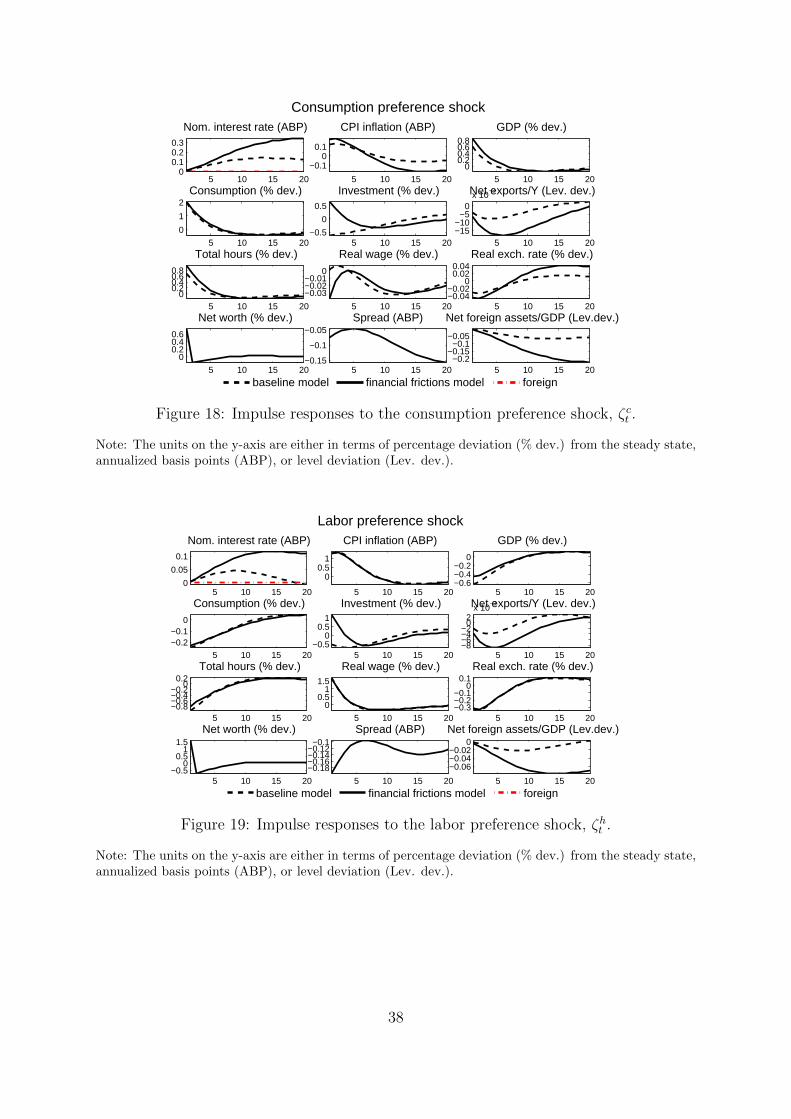
Consumption preference shock


−0.2−0.15

−0.1−0.05


5 10 15 20−0.15

−0.1

−0.05Spread (ABP)

5 10 15 20

00.20.40.6

Net worth (% dev.)5 10 15 20

−0.04−0.02

00.020.04


5 10 15 20

−0.03−0.02−0.01

0

Real wage (% dev.)

5 10 15 200

0.20.40.60.8


−15−10

−50


5 10 15 20−0.5

0

0.5

Investment (% dev.)

5 10 15 20

0

1

2Consumption (% dev.)

5 10 15 20

00.20.40.60.8

GDP (% dev.)

5 10 15 20

−0.10

0.1

CPI inflation (ABP)

5 10 15 200

0.10.20.3


Figure 18: Impulse responses to the consumption preference shock, ζct .


Labor preference shock


−0.06−0.04−0.02

0Net foreign assets/GDP (Lev.dev.)

5 10 15 20

−0.18−0.16−0.14−0.12

−0.1Spread (ABP)

5 10 15 20−0.5

00.5

11.5

Net worth (% dev.)5 10 15 20

−0.3−0.2−0.1

00.1


5 10 15 20

00.5

11.5

Real wage (% dev.)

5 10 15 20−0.8−0.6−0.4−0.2

00.2


−8−6−4−2

02


5 10 15 20−0.5

00.5

1

Investment (% dev.)

5 10 15 20−0.2−0.1

0


−0.6−0.4−0.2

0

GDP (% dev.)

5 10 15 20

00.5

1

CPI inflation (ABP)

5 10 15 200

0.05

0.1


Figure 19: Impulse responses to the labor preference shock, ζht .


38

Government consumption shock


−6−4−2


5 10 15 20

−0.02

−0.01

Spread (ABP)

5 10 15 20

0

0.1

0.2Net worth (% dev.)

5 10 15 20

−10−5

0


5 10 15 20

00.010.02

Real wage (% dev.)

5 10 15 20−0.2

00.20.40.60.8


−10−5

0x 10

−4Net exports/Y (Lev. dev.)

5 10 15 20

00.05

0.1

Investment (% dev.)

5 10 15 20−10

−50

x 10−3Consumption (% dev.)

5 10 15 20−0.2

00.20.40.60.8

GDP (% dev.)

5 10 15 20

00.020.04

CPI inflation (ABP)

5 10 15 20

2468

10x 10

−3Nom. interest rate (ABP)

Figure 20: Impulse responses to the government consumption shock, gt.

Note: The units on the y-axis are either in terms of percentage deviation (% dev.) from the steadystate, annualized basis points (ABP), or level deviation (Lev. dev.). In this model, the governmentconsumption crowds out the private consumption. Total consumption falls due to the worsening of thenet foreign assets position and a subsequent increase in the risk premium to the nominal interest ratethat makes saving activity more appealing.

Domestic markup shock


−8−6−4−2

02


5 10 15 20

−0.04

−0.02

Spread (ABP)

5 10 15 20−1

−0.50

Net worth (% dev.)5 10 15 20

−0.8−0.6−0.4−0.2

0


5 10 15 20−1.5

−1−0.5

0

Real wage (% dev.)

5 10 15 20−0.6−0.4−0.2

0


−2−1

01


5 10 15 20

−0.4−0.2

0

Investment (% dev.)

5 10 15 20−0.08−0.06−0.04−0.02

0


−0.4−0.2

0

GDP (% dev.)

5 10 15 200123

CPI inflation (ABP)

5 10 15 20−5

05

10x 10


Figure 21: Impulse responses to the domestic markup shock, τ dt .


39

Import export markup shock


0.02

0.04


5 10 15 20−0.08−0.06−0.04−0.02

0

Spread (ABP)

5 10 15 20

00.20.40.6

Net worth (% dev.)5 10 15 20

−0.04

−0.02

0


5 10 15 200

0.050.1

Real wage (% dev.)

5 10 15 20−1

0123


00.010.02


5 10 15 200

0.20.40.6

Investment (% dev.)

5 10 15 200

0.020.040.06


−1012

GDP (% dev.)

5 10 15 200

0.050.1

0.15

CPI inflation (ABP)

5 10 15 20−0.1

−0.08−0.06−0.04−0.02


Figure 22: Impulse responses to the imported export markup shock, τmxt .


Import consumption markup shock


0.010.015

0.02


5 10 15 20

−0.04−0.02

0

Spread (ABP)

5 10 15 20

00.20.4

Net worth (% dev.)5 10 15 20

−1.5−1

−0.50


5 10 15 20

00.10.20.3

Real wage (% dev.)

5 10 15 20−0.2

00.20.40.60.8


024


5 10 15 200

0.10.20.3

Investment (% dev.)

5 10 15 20−0.1

−0.050


00.20.40.6

GDP (% dev.)

5 10 15 20

0246

CPI inflation (ABP)

5 10 15 20−0.04

−0.02

0Nom. interest rate (ABP)

Figure 23: Impulse responses to the import consumption markup shock, τmct .


40

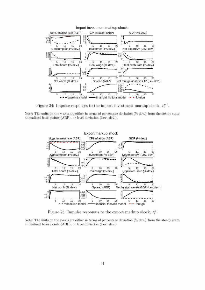
Import investment markup shock


0.020.040.060.08


5 10 15 20

−0.4−0.2

0Spread (ABP)

5 10 15 200

2

4Net worth (% dev.)

5 10 15 20−0.2

−0.1

0


5 10 15 20

−0.1−0.05

0

Real wage (% dev.)

5 10 15 20−1

0123


00.010.02


5 10 15 20−4−2

0

Investment (% dev.)

5 10 15 20

00.020.040.06


−1012

GDP (% dev.)

5 10 15 200

0.20.40.60.8

CPI inflation (ABP)

5 10 15 20

−0.15−0.1

−0.050Nom. interest rate (ABP)

Figure 24: Impulse responses to the import investment markup shock, τmit .


Export markup shock


024


5 10 15 200.01

0.0150.02

0.025

Spread (ABP)

5 10 15 20

−0.2−0.1

0

Net worth (% dev.)5 10 15 20

−505

1015


5 10 15 20−0.03−0.02−0.01

0

Real wage (% dev.)

5 10 15 20−0.6−0.4−0.2

0


−20246


5 10 15 20−0.2−0.1

0

Investment (% dev.)

5 10 15 20−2

02468


5 10 15 20

−0.4−0.2

0

GDP (% dev.)

5 10 15 20−0.06−0.04−0.02

00.02

CPI inflation (ABP)

5 10 15 20−6−4−2

0x 10


Figure 25: Impulse responses to the export markup shock, τxt .


41

Unit−root technology shock


0.020.040.06


5 10 15 20−0.04−0.02

00.02

Spread (ABP)

5 10 15 20

−0.3−0.2−0.1

00.1

Net worth (% dev.)5 10 15 20

−0.020

0.020.040.06


5 10 15 20

0.020.040.06

Real wage (% dev.)

5 10 15 20

−0.020

0.02Total hours (% dev.)

5 10 15 20024


5 10 15 20

−0.4−0.2

0

Investment (% dev.)

5 10 15 200

0.010.020.03


00.05

0.1

GDP (% dev.)

5 10 15 20−0.1

−0.05

0

CPI inflation (ABP)

5 10 15 200.05

0.10.15

0.20.25


Figure 26: Impulse responses to the unit-root technology shock, µz,t.


Foreign inflation shock


123


5 10 15 20−6

−4

−2x 10

−3Spread (ABP)

5 10 15 200

0.010.020.03

Net worth (% dev.)5 10 15 20

00.020.04


5 10 15 20

−15−10

−505

x 10−4Real wage (% dev.)

5 10 15 20

01020

x 10−3Total hours (% dev.)

5 10 15 20

0123


5 10 15 20

−0.03−0.02−0.01

00.01

Investment (% dev.)

5 10 15 20

−2−1

0


5 10 15 20

01020

x 10−3GDP (% dev.)

5 10 15 200

0.020.04

CPI inflation (ABP)

5 10 15 200

0.020.040.060.08


Figure 27: Impulse responses to the foreign inflation shock, επ∗,t.

Note: The units on the y-axis are either in terms of percentage deviation (% dev.) from the steady state,annualized basis points (ABP), or level deviation (Lev. dev.). A temporary positive shock to foreigninflation causes the cost of imported consumption and investment to rise. As a result, consumption andinvestment decrease, imports decrease, and GDP goes up. The effects are small in magnitude, though.

42

0.2 0.4 0.6 0.8 1 1.2 1.40

2

4

6

8

SE_muz_eps

0 1 20

2

4

6

SE_ystar_eps

0 1 20

1

2

3

4

SE_pistar_eps

0.1 0.2 0.3 0.40

20

40

60SE_Rstar_eps

0.2 0.4 0.6 0.80

2

4

6

rhomuz

0.7 0.8 0.9 10

5

10

a11

0.4 0.6 0.80

2

4

6

8

a22

0.7 0.8 0.9 10

5

10

15

a33

−0.6−0.4−0.2 0 0.2 0.40

1

2

3

4

a12

Figure 28: SVAR priors and posteriors.

Note: Prior distribution in gray, simulated distribution in black, and the computed posterior mode indashed green.

−0.4 −0.2 0 0.20

2

4

6

8

a13

−0.2 0 0.2 0.4 0.60

2

4

6

8

a21

−0.4 −0.2 0 0.20

2

4

6

8

a23

−0.2 0 0.2 0.40

5

10

a24

−0.2 0 0.20

5

10

15

a31

−0.4 −0.2 0 0.20

2

4

6

a32

−0.2 0 0.2 0.40

5

10

15

a34

−0.2 0 0.20

5

10

c21

0 0.1 0.2 0.30

5

10

c31

Figure 29: SVAR priors and posteriors (continued).


43

0.2 0.4 0.60

2

4

6

8

c32

−0.2 0 0.20

5

10

c24

−0.1 0 0.1 0.20

5

10

c34

Figure 30: SVAR priors and posteriors (continued).


0.2 0.4 0.6 0.80

10

20

SE_epsilon_eps

0 0.2 0.4 0.6 0.80

5

10

SE_Upsilon_eps

0 0.2 0.4 0.6 0.80

5

10

SE_zetac_eps

0 1 2 30

1

2

3

SE_zetah_eps

0.5 1 1.5 2 2.50

2

4

6

8

SE_phitilde_eps

0.5 1 1.5 2 2.50

5

10SE_g_eps

0 1 20

2

4

SE_taud_eps

0 2 40

1

2

3

SE_taux_eps

0 1 2 30

1

2

3

SE_taumc_eps

Figure 31: Priors and posteriors.

Note: Financial frictions model. Prior distribution in gray, simulated distribution in black, and thecomputed posterior mode in dashed green.

44

0 1 20

2

4

SE_taumi_eps

0 2 4 60

1

2

3

SE_taumx_eps

0.5 1 1.5 2 2.50

5

10SE_gamma_eps

0.5 0.6 0.7 0.8 0.90

5

10

15

xid

0.6 0.8 10

5

10

15

xix

0.5 0.6 0.7 0.8 0.90

2

4

6

8

ximc

0.2 0.4 0.6 0.80

2

4

6

8

ximi

0.4 0.6 0.80

2

4

ximx

0 0.2 0.4 0.6 0.80

2

4

kappad

Figure 32: Priors and posteriors (continued).


0 0.5 10

1

2

3

4kappax

0 0.5 10

1

2

3

kappamc

0 0.5 10

1

2

3

4kappami

0 0.5 10

1

2

3kappamx

−0.2 0 0.2 0.4 0.6 0.80

1

2

3

4

kappaw

0 0.5 10

0.5

1

1.5work_cap_para

0 0.2 0.4 0.6 0.80

1

2

3

4

sigmaLScaled

0.2 0.4 0.6 0.8 10

5

10

b

0 0.5 10

5

10

SppScaled



45

0 0.5 10

2

4

6

sigmaa

1 1.5 2 2.50

0.5

1

1.5

2etax

1 1.5 20

0.5

1

1.5

2

etac

1 2 30

0.5

1

1.5

etaf

0.1 0.2 0.3 0.4 0.50

5

10

mu

0.6 0.8 10

2

4

6

8rhoepsilon

0.2 0.4 0.6 0.8 10

2

4

6rhoUpsilon

0.6 0.8 10

2

4

6

8

rhozetac

0.4 0.6 0.8 10

2

4

6

rhozetah



0.6 0.8 10

5

10

15

rhophitilde

0.2 0.4 0.6 0.8 10

2

4

6rhog

0.2 0.4 0.6 0.8 10

2

4

6rhogamma



Appendix C The model

C.1 The baseline model

As described in Section 2, the three final goods - consumption, investment and exports - are producedby combining the domestic homogeneous good with specific imported inputs for each type of final good.Below we start the model description by going through the production of all these goods.

C.1.1 Production of the domestic homogeneous good

A homogeneous domestic good, Yt, is produced using

Yt =

[∫ 1

0

Y1/λdi,t di

]λd, 1 ≤ λd <∞, (C.1)

46

where Yi,t denotes intermediate goods and 1/λd their degree of substitutability. The homogeneousdomestic good is produced by a competitive, representative firm which takes the price of output, Pt, andthe price of inputs, Pi,t, as given.

The i-th intermediate good producer has the following production function:

Yi,t = (ztHi,t)1−αεtK

αi,t − z+

t φ, (C.2)

where Ki,t denotes the capital services rented by the i-th intermediate good producer. Also, log zt isa technology shock whose first difference has a positive mean, log εt is a stationary neutral technologyshock and φ denotes a fixed production cost. The economy has two sources of growth: the positive driftin log zt and a positive drift in log Ψt, where Ψt is an investment-specific technology shock. The objectz+t in (C.2) is defined as13

z+t = Ψ

α1−αt zt.

In (C.2), Hi,t denotes homogeneous labor services hired by the i-th intermediate good producer.Firms must borrow a fraction νf of the wage bill, so that one unit of labor costs is denoted by

WtRft ,

withRft = νfRt + 1− νf , (C.3)

where Wt is the aggregate wage rate, and Rt is the risk-free interest rate that apply on working capitalloans.

The firm’s marginal cost, divided by the price of the homogeneous good is denoted by mct:

mct = τdt

(1

1− α

)1−α(1

α

)α (rkt)α (

wtRft

)1−α 1

εt, (C.4)

where rkt is the nominal rental rate of capital scaled by Pt and wt = Wt/(z+t Pt). Also, τdt is a tax-like

shock which affects marginal cost but does not appear in a production function.14

Productive efficiency dictates that marginal cost is equal to the cost of producing another unit usinglabor, implying:

mct = τdt(µΨ,t)

αwtR

ft

εt(1− α)(

ki,tµz+,tHi,t

)α (C.5)

The i-th firm is a monopolist in the production of the i-th good and so it sets its price. Price settingis subject to Calvo frictions. With probability ξd the intermediate good firm cannot reoptimize its price,in which case,

Pi,t = πd,tPi,t−1, πd,t := (πt−1)κd(πct )1−κd−κd(π)κd ,

where κd, κd, κd + κd ∈ (0, 1) are parameters, πt−1 is the lagged inflation rate and πct is the centralbank’s (implicit) target inflation rate. Also, π is a scalar which allowing to capture, among other things,the case in which non-optimizing firms either do not change price at all (i.e., π = κd = 1) or that theyindex only to the steady state inflation rate (i.e., π = π, κd = 1). Note that there is a price dispersionin steady state if κd > 0 and if π is different from the steady state value of π.

With probability 1−ξd the firm can change the price. The problem of the i-th domestic intermediategood producer which has the opportunity to change price is to maximize discounted profits:

Et

∞∑j=0

βjυt+j {Pi,t+jYi,t+j −mct+jPt+jYi,t+j} , (C.6)

13The details regarding the scaling of variables are collected in Appendix D.14In the linearized version of the model in which there are no price and wage distortions in the steady

state, τdt is isomorphic to a disturbance in λd, i.e., a markup shock.

47

subject to the requirement that production equals demand. In the above expression, υt is the multiplieron the household’s nominal budget constraint. It measures the marginal value to the household of oneunit of profits in terms of currency. In states of nature when the firm can reoptimize price, it does soto maximize its discounted profits subject to the price setting frictions and to the requirement that itsatisfies demand given by (

PtPi,t

) λdλd−1

Yt = Yi,t. (C.7)

The equilibrium conditions associated with the price setting problem and their derivation are reportedin Appendix D.

The domestic intermediate output good is allocated among alternative uses as follows:

Yt = Gt + Cdt + Idt +

∫ 1

0

Xdi,tdi, (C.8)

where Gt denotes government consumption (which consists entirely of the domestic good), Cdt denotesintermediate goods used (together with foreign consumption goods) to produce final household consump-tion goods, Idt is the amount of intermediate domestic goods used in combination with imported foreigninvestment goods to produce a homogeneous investment good. Finally, the integral in (C.8) denotesdomestic resources allocated to exports. The determination of consumption, investment and exportdemand is discussed below.

C.1.2 Production of final consumption and investment goods

Final consumption goods are purchased by households. These goods are produced by a representativecompetitive firm using the following linear homogeneous technology:

Ct =

[(1− ωc)

1ηc

(Cdt) ηc−1

ηc + ω1ηcc (Cmt )

ηc−1ηc

] ηcηc−1

. (C.9)

The representative firm takes the price of final consumption goods output, P ct , as given. Finalconsumption goods output is produced using two inputs. The first, Cdt , is a one-for-one transformationof the homogeneous domestic good and therefore has price, Pt. The second input, Cmt , is the homogeneouscomposite of specialized consumption import goods discussed in the next subsection. The price of Cmt isPm,ct . The representative firm takes the input prices, Pt and Pm,ct as given. Profit maximization leadsto the following demand for the intermediate inputs in a scaled form:

cdt = (1− ωc)(pct)ηcct

cmt = ωc

(pctpm,ct

)ηcct, (C.10)

where pct = P ct /Pt and pm,ct = Pm,ct /Pt. The price of Ct is related to the price of the inputs by

pct =[(1− ωc) + ωc(p

m,ct )1−ηc

] 11−ηc . (C.11)

The rate of inflation of the consumption good is

πct =P ctP ct−1

= πt

[(1− ωc) + ωc(p

m,ct )1−ηc

(1− ωc) + ωc(pm,ct−1)1−ηc

] 11−ηc

. (C.12)

Investment goods are produced by a representative competitive firm using the following technology:

It + a(ut)Kt = Ψt

[(1− ωi)

1ηi

(Idt) ηi−1

ηi + ω1ηii (Imt )

ηi−1

ηi

] ηiηi−1

,

where investment is defined as the sum of investment goods, It, used in the accumulation of physicalcapital plus investment goods used in capital maintenance, a(ut)Kt. The maintenance is discussed below.

48

See Appendix D for the functional form of a(ut). ut denotes the utilization rate of capital, with capitalservices being defined by

Kt = utKt.

In order to accommodate the possibility that the price of investment goods relative to the price ofconsumption goods declines over time, it is assumed that the investment specific technology shock Ψt is aunit root process with a potentially positive drift. As in the consumption good sector, the representativeinvestment goods producers take all relevant prices as given. Profit maximization leads to the followingdemand for the intermediate inputs in a scaled form:

idt =(pit)ηi (

it + a(ut)kt

µψ,tµz+,t

)(1− ωi) (C.13)

imt = ωi

(pit

pm,it

)ηi (it + a(ut)

ktµψ,tµz+,t

)(C.14)

where pit = ΨtPit /Pt and pm,it = Pm,it /Pt.

The price of It is related to the price of the inputs by

pit =[(1− ωi) + ωi(p

m,it )1−ηi

] 11−ηi

. (C.15)

The rate of inflation of the investment good is

πit =πtµΨ,t

(1− ωi) + ωi

(pm,it

)1−ηi

(1− ωi) + ωi

(pm,it−1

)1−ηi

1

1−ηi

. (C.16)

C.1.3 Exports and imports

Both exports and imports activities involve Calvo price setting frictions and therefore require the presenceof market power. Dixit-Stiglitz strategy is used to introduce a range of specialized goods. This allowsthere to be market power without the counterfactual implication that there is a small number of firmsin the export and import sector. Thus, exports involve a continuum of exporters, each of which isa monopolist which produces a specialized export good. Each monopolist produces the export goodusing a homogeneous domestically produced good and a homogeneous good derived from imports. Thespecialized export goods are sold to foreign competitive retailers which create a homogeneous good thatis sold to foreign citizens.

In the case of imports, specialized domestic importers purchase a homogeneous foreign good whichthey turn into a specialized input and sell to domestic retailers. There are three types of domesticretailers. One uses the specialized import goods to create the homogeneous good used as an input intothe production of specialized exports. Another uses the specialized import goods to create an input usedin the production of investment goods. The third type uses specialized imports to produce a homogeneousinput used in the production of consumption goods. Imported goods are combined with domestic inputsbefore being passed on to final domestic users. There are pricing frictions in both exports and imports.In all cases it is assumed that prices are set in the currency of the buyer (‘pricing to market’).15

Exports. There is a total demand by foreigners for domestic exports, which takes on the followingform:

15Pricing frictions in imports help the model account for the evidence that exchange rate shocks taketime to pass into domestic prices. Pricing frictions in exports help the model to produce a hump-shapein the response of output to a domestic monetary shock, though, as seen in Section 4, it is not the casefor a currency area-wide monetary policy shock.

49

Xt =

(P xtP ∗t

)−ηfY ∗t , (C.17)

where Y ∗t is foreign GDP, P ∗t is the foreign currency price of foreign homogeneous goods and P xt is anindex of export prices defined below. The goods Xt are produced by a representative competitive foreignretailer firm using specialized inputs as follows:

Xt =

[∫ 1

0

X1λxi,t di

]λx, (C.18)

where Xi,t, i ∈ (0, 1) are specialized intermediate goods for export good production. The retailerthat produces Xt takes its output price P xt and its input prices P xi,t as given. Optimization leads to thefollowing demand for specialized exports:

Xi,t =

(P xi,tP xt

) −λxλx−1

Xt. (C.19)

Combining (C.18) and (C.19),

P xt =

[∫ 1

0

(P xi,t) 1

1−λx di

]1−λx

.

The i-th specialized export is produced by a monopolist using the following technology:

Xi,t =

[ω

1ηxx

(Xmi,t

) ηx−1ηx + (1− ωx)

1ηx

(Xdi,t

) ηx−1ηx

] ηxηx−1

,

where Xmi,t and Xd

i,t are the i-th exporter’s use of the imported and domestically produced goods, re-spectively. The marginal cost associated with the CES production function is derived from the multiplierassociated with the Lagrangian representation of the cost minimization problem:

C = min τxt[Pm,xt RxtX

mi,t + PtR

xtX

di,t

]+ λ

{Xi,t −

[ω

1ηxx

(Xmi,t

) ηx−1ηx + (1− ωx)

1ηx

(Xdi,t

) ηx−1ηx

] ηxηx−1

},

where Pm,xt is the price of the homogeneous import good and Pt is the price of the homogeneous domesticgood. Using the first order conditions of this problem and the production function, the real marginalcost in terms of stationary variables, mcxt , is derived as

mcxt =λ

StP xt=

τxt Rxt

qtpctpxt

[ωx (pm,xt )

1−ηx + (1− ωx)] 1

1−ηx, (C.20)

whereRxt = νxRt + 1− νx, (C.21)

StPxt

Pt=StP

∗t

P ct

P ctPt

P xtP ∗t

= qtpctpxt , (C.22)

and qt denotes the real exchange rate defined as

qt =StP

∗t

P ct. (C.23)

From the solution to the same problem, the demand for domestic inputs for export production is

Xdi,t =

(λ

τxt Rxt Pt

)ηxXi,t(1− ωx). (C.24)

The quantity of the domestic homogeneous good used by specialized exporters is

50

∫ 1

0

Xdi,tdi,

which, in terms of aggregates, is [by plugging (C.24) into this integral and derived in Appendix D]

Xdt =

∫ 1

0

Xdi,tdi =

[ωx(pm,xt )1−ηx + (1− ωx)

] ηx1−ηx (1− ωx)(pxt )

−λxλx−1 (pxt )−ηfY ∗t (C.25)

where pxt is a measure of the price dispersion and is defined in Appendix D.Using a similar derivation as for Xd

t ,

Xmt = ωx

[ωx(pm,xt )1−ηx + (1− ωx)] 1

1−ηx

pm,xt

ηx

(pxt )−λxλx−1 (pxt )−ηfY ∗t . (C.26)

The i-th, i ∈ (0, 1), export good firm takes (C.19) as its demand curve. This producer sets pricessubject to a Calvo sticky-price mechanism. With probability ξx, the i-th export good firm cannotreoptimize its price, in which case it updates the price as follows:

P xi,t = πxt Pxi,t−1, π

xt = (πxt−1)κx(πx)1−κx−κx(π)κx , (C.27)

where κx, κx, κx + κx ∈ (0, 1).The equilibrium conditions associated with price setting by exporters that do get to reoptimize their

prices are analogous to the ones derived for the domestic intermediate good producers and are reportedin Appendix D.

Imports. Foreign firms sell a homogeneous good to domestic importers. The importers convert thehomogeneous good into a specialized input (‘brand name it’) and supply that input monopolisticallyto domestic retailers. Importers are subject to Calvo price setting frictions. There are three typesof importing firms: (i) one produces goods used to produce an intermediate good for the productionof consumption, (ii) one produces goods used to produce an intermediate good for the production ofinvestment, and (iii) one produces goods used to produce an intermediate good for the production ofexports.

Consider (i) first. The production function of the domestic retailer of imported consumption goodsis

Cmt =

[∫ 1

0

(Cmi,t)1

λm,c di

]λm,c,

where Cmi,t is the output of the i-th specialized producer and Cmt is an intermediate good used in theproduction of the consumption goods. Let Pm,ct denote the price index of Cmt and let Pm,ci,t denote theprice of the i-th intermediate input. The domestic retailer is competitive and takes Pm,ct and Pm,ci,t asgiven. The demand curve for specialized inputs is given by the domestic retailer’s first order necessarycondition for profit maximization:

Cmi,t = Cmt

(Pm,ct

Pm,ci,t

) λm,cλm,c−1

.

We now turn to the producer of Cmi,t who takes the previous equation as a demand curve. Thisproducer buys the homogeneous foreign good and converts it one-for-one into the domestic differentiatedgood, Cmi,t. The intermediate good producer’s marginal cost is

τm,ct StP∗t R

ν,∗t , (C.28)

whereRν,∗t = ν∗R∗t + 1− ν∗, (C.29)

51

where R∗t is the foreign nominal rate of interest.16

As in the homogeneous domestic good sector, τm,ct is a tax-like shock which affects marginal costsbut does not appear in a production function.17

The total value of imports accounted for by the consumption sector is

StP∗t R

ν,∗t Cmt (pm,ct )

λm,c1−λm,c ,

where

pm,ct =Pm,ct

Pm,ct

is a measure of the price dispersion in the differentiated good, Cmi,t.Now consider (ii). The production function for the domestic retailer of imported investment goods,

Imt , is

Imt =

[∫ 1

0

(Imi,t)1

λm,i di

]λm,i.

The retailer of imported investment goods is competitive and takes output prices, Pm,it , and input prices,Pm,ii,t , as given.

The producer of the i-th intermediate input into the above production function buys the homogeneousforeign good and converts it one-for-one into the differentiated good, Imi,t. The marginal cost of Imi,t is theanalogue of (C.28):

τm,it StP∗t R

ν,∗t ,

which implies the importing firm’s cost is P ∗t (before borrowing costs, exchange rate conversion andmarkup shocks), which is the same cost for the specialized inputs used to produce Cmt .

The total value of imports associated with the production of investment goods is analogous to whatwas obtained for the consumption good sector:

StP∗t R

ν,∗t Imt (pm,it )

λm,i1−λm,i , pm,it =

Pm,ii,t

Pm,it

. (C.30)

Now consider (iii). The production function of the domestic retailer of imported goods used in theproduction of an input, Xm

t , for the production of export goods is

Xmt =

[∫ 1

0

(Xmi,t)

1λm,x di

]λm,x.

The imported good retailer is competitive and takes output prices, Pm,xt , and input prices, Pm,xi,t , asgiven. The producer of the specialized input, Xm

i,t, has marginal cost

τm,xt StP∗t R

ν,∗t .

The total value of imports associated with the production of Xmt is

StP∗t R

ν,∗t Xm

t (pm,xt )λm,x

1−λm,x , pm,xt =Pm,xi,t

Pm,xt

. (C.31)

16The notion here is that the intermediate good firm must pay the inputs with foreign currency andbecause they have no resources themselves at the beginning of the period, they must borrow thoseresources if they are to buy the foreign inputs needed to produce Cmi,t. The financing need is in theforeign currency, so the loan is taken in that currency. There is no risk to this working capital loanbecause all shocks are realized at the beginning of the period and so there is no uncertainty within theduration of the loan about the realization of prices and exchange rates.

17In the linearization of a version of the model in which there are no price and wage distortions in thesteady state, τm,ct is isomorphic to a markup shock.

52

Each of the above three types of intermediate good firm is subject to Calvo price-setting frictions.With probability 1 − ξm,j , the j-th type of firm can reoptimize its price and with probability ξm,j itupdates its price according to

Pm,ji,t = πm,jt Pm,ji,t−1, πm,jt := (πm,jt−1)κm,j (πct )

1−κm,j−κm,j πκm,j , j = c, i, x. (C.32)

The equilibrium conditions associated with price setting by importers are analogous to the onesderived for domestic intermediate good producers and are reported in Appendix D.

C.1.4 Households

Household preferences are given by

Ej0

∞∑t=0

βt[ζct log(Ct − bCt−1)− ζht AL

(hj,t)1+σL

1 + σL

], (C.33)

where ζct denotes a consumption preference shock, ζht a disutility of labor shock, b is the consumptionhabit parameter, hj denotes the j-th household’s supply of labor services and σL denotes the inverseFrisch elasticity. The household owns the economy’s stock of physical capital. It determines the rate atwhich the capital stock is accumulated and the rate at which it is utilized. The household also owns thestock of net foreign assets and determines its rate of accumulation.

Wage setting. The specialized labor supplied by households is combined by labor contractors intoa homogeneous labor services:

Ht =

[∫ 1

0

(hj,t)1λw dj

]λw, 1 ≤ λw <∞.

Households are subject to Calvo wage setting frictions (as in Erceg, Henderson and Levin, 2000).With probability 1 − ξw the j-th household is able to reoptimize its wage and with probability ξw itupdates its wage according to

Wj,t+1 = πw,t+1Wj,t (C.34)

πw,t+1 = (πct )κw(πct+1

)1−κw−κw(π)κw(µz+)ϑw , (C.35)

where κw, κw, ϑw, κw + κw ∈ (0, 1).Consider the jth household that has an opportunity to reoptimize its wage at time t. Denote this

wage rate by Wt. This is not indexed by j because the situation of each household that optimizes itswage is the same. In choosing Wt the household considers the discounted utility (neglecting currentlyirrelevant terms in the household objective) of future histories when it cannot reoptimize (note the i vsj):

Ejt

∞∑i=0

(βξw)i

[−ζht+iAL

(hj,t+i)1+σL

1 + σL+ υt+iWj,t+ihj,t+i

1− τy

1 + τw

], (C.36)

where τy is a tax on labor income, τw is a payroll tax, υt is the multiplier on the household’s period tbudget constraint. The demand for the jth household’s labor services, conditional on it having optimizedin period t and not again since, is

hj,t+i =

(Wtπw,t+i, · · · , πw,t+1

Wt+i

) λw1−λw

Ht+i, (C.37)

where it is understood that πw,t+i, · · · , πw,t+1 = 1 when i = 0. The equilibrium conditions associatedwith this problem, i.e. wage setting of households that do get to reoptimize, are reported in AppendixD.

53

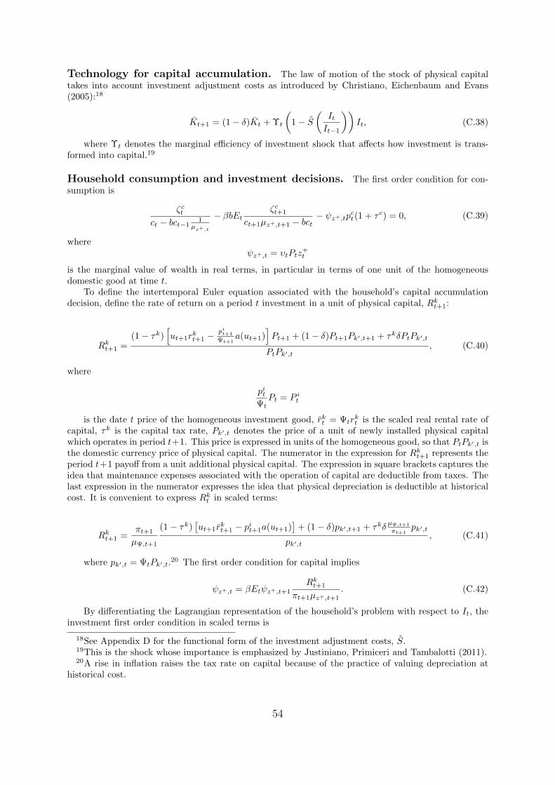
Technology for capital accumulation. The law of motion of the stock of physical capitaltakes into account investment adjustment costs as introduced by Christiano, Eichenbaum and Evans(2005):18

Kt+1 = (1− δ)Kt + Υt

(1− S

(ItIt−1

))It, (C.38)

where Υt denotes the marginal efficiency of investment shock that affects how investment is trans-formed into capital.19

Household consumption and investment decisions. The first order condition for con-sumption is

ζctct − bct−1

1µz+,t

− βbEtζct+1

ct+1µz+,t+1 − bct− ψz+,tp

ct(1 + τ c) = 0, (C.39)

whereψz+,t = υtPtz

+t

is the marginal value of wealth in real terms, in particular in terms of one unit of the homogeneousdomestic good at time t.

To define the intertemporal Euler equation associated with the household’s capital accumulationdecision, define the rate of return on a period t investment in a unit of physical capital, Rkt+1:

Rkt+1 =(1− τk)

[ut+1r

kt+1 −

pit+1

Ψt+1a(ut+1)

]Pt+1 + (1− δ)Pt+1Pk′,t+1 + τkδPtPk′,t

PtPk′,t, (C.40)

where

pitΨtPt = P it

is the date t price of the homogeneous investment good, rkt = Ψtrkt is the scaled real rental rate of

capital, τk is the capital tax rate, Pk′,t denotes the price of a unit of newly installed physical capitalwhich operates in period t+1. This price is expressed in units of the homogeneous good, so that PtPk′,t isthe domestic currency price of physical capital. The numerator in the expression for Rkt+1 represents theperiod t+1 payoff from a unit additional physical capital. The expression in square brackets captures theidea that maintenance expenses associated with the operation of capital are deductible from taxes. Thelast expression in the numerator expresses the idea that physical depreciation is deductible at historicalcost. It is convenient to express Rkt in scaled terms:

Rkt+1 =πt+1

µΨ,t+1

(1− τk)[ut+1r

kt+1 − pit+1a(ut+1)

]+ (1− δ)pk′,t+1 + τkδ

µΨ,t+1

πt+1pk′,t

pk′,t, (C.41)

where pk′,t = ΨtPk′,t.20 The first order condition for capital implies

ψz+,t = βEtψz+,t+1

Rkt+1

πt+1µz+,t+1. (C.42)

By differentiating the Lagrangian representation of the household’s problem with respect to It, theinvestment first order condition in scaled terms is

18See Appendix D for the functional form of the investment adjustment costs, S.19This is the shock whose importance is emphasized by Justiniano, Primiceri and Tambalotti (2011).20A rise in inflation raises the tax rate on capital because of the practice of valuing depreciation at

historical cost.

54

−ψz+,tpit+ψz+,tpk′,tΥt

[1− S

(µz+,tµΨ,tit

it−1

)− S′

(µz+,tµΨ,tit

it−1

)µz+,tµΨ,tit

it−1

]+ βψz+,t+1pk′,t+1Υt+1S

′(µz+,t+1µΨ,t+1it+1

it

)(it+1

it

)2

µΨ,t+1µz+,t+1 = 0. (C.43)

The first order condition associated with capital utilization is, in scaled terms21

rkt = pita′(ut). (C.44)

Financial assets. The household does the domestic economy’s saving. Period t saving occurs bythe acquisition of net foreign assets, A∗t+1, and a domestic asset. The domestic asset is used to financethe working capital requirements of firms. This asset pays a nominally non-state contingent return fromt to t+ 1, Rt. The first order condition associated with this domestic asset is


µz+,t+1

[Rt − τ b(Rt − πt+1)

πt+1

], (C.45)

where τ b is the tax rate on the real interest rate on bond income.22

The tax treatment of domestic agent’s earnings on foreign bonds is the same as the tax treatmentof agent’s earnings on domestic bonds. The date t first order condition associated with the asset A∗t+1

that pays R∗t in terms of foreign currency is

υtSt = βEtυt+1

[St+1R

∗tΦt − τ b

(St+1R

∗tΦt −

StPtPt+1

)]. (C.46)

Recall that St is the domestic currency price of a unit foreign currency. The left side of this expressionis the cost of acquiring a unit of foreign assets. The currency cost is St and this is converted into utilityterms by multiplying by the multiplier on the household’s budget constraint, υt. The term in squarebrackets is the after-tax payoff of the foreign asset in domestic currency units. The period t+ 1 pre-taxinterest payoff on A∗t+1 is St+1R

∗tΦt. Here, R∗t is the foreign nominal rate of interest, which is risk

free in foreign currency units. The term Φt represents a relative risk adjustment of the foreign assetreturn, so that a unit of the foreign asset acquired in t pays off R∗tΦt units of foreign currency in t+ 1.The determination of Φt is discussed below. The remaining term in brackets pertains to the impact oftaxation on returns on foreign assets.23

Scaling the first order condition, (C.46), by multiplying both sides by Ptz+t /St yields


πt+1µz+,t+1

[st+1R

∗tΦt − τ b(st+1R

∗tΦt − πt+1)

], (C.47)

where

st =StSt−1

.

The risk adjustment term has the following form:

Φt = Φ(at, R

∗t −Rt, φt

)= exp

(−φa(at − a)− φs(R∗t −Rt − (R∗ −R)) + φt

), (C.48)

21The tax rate on capital income does not enter here because of the deductibility of maintenance costs.22A consequence of this treatment of the taxation on domestic bonds is that the steady state real

after-tax return on bonds is invariant to π.23If we ignore the term after the minus sign in parentheses, then the taxation is applied to the whole

nominal payoff on the bond, including principal. The term after the minus sign is designed to ensurethat the principal is deducted from taxes. The principal is expressed in nominal terms and is set so thatthe real value at t+ 1 coincides with the real value of the currency used to purchase the asset in periodt. Recall that St is the period t domestic currency cost of a unit (in terms of foreign currency) of foreignassets. So the period t real cost of the asset is St/Pt. The domestic currency value in period t+ 1 of thisreal quantity is Pt+1St/Pt.

55

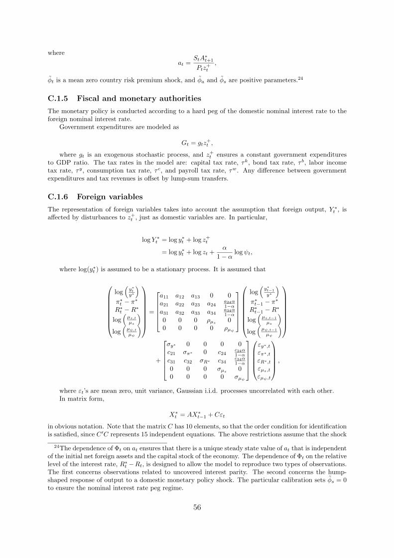
where

at =StA

∗t+1

Ptz+t

,

φt is a mean zero country risk premium shock, and φa and φs are positive parameters.24

C.1.5 Fiscal and monetary authorities

The monetary policy is conducted according to a hard peg of the domestic nominal interest rate to theforeign nominal interest rate.

Government expenditures are modeled as

Gt = gtz+t ,

where gt is an exogenous stochastic process, and z+t ensures a constant government expenditures

to GDP ratio. The tax rates in the model are: capital tax rate, τk, bond tax rate, τ b, labor incometax rate, τy, consumption tax rate, τ c, and payroll tax rate, τw. Any difference between governmentexpenditures and tax revenues is offset by lump-sum transfers.

C.1.6 Foreign variables

The representation of foreign variables takes into account the assumption that foreign output, Y ∗t , isaffected by disturbances to z+

t , just as domestic variables are. In particular,

log Y ∗t = log y∗t + log z+t

= log y∗t + log zt +α

1− αlogψt,

where log(y∗t ) is assumed to be a stationary process. It is assumed that

log(y∗ty∗

)π∗t − π∗R∗t −R∗

log(µz,tµz

)log(µψ,tµψ

)

=

a11 a12 a13 0 0a21 a22 a23 a24

a24α1−α

a31 a32 a33 a34a34α1−α

0 0 0 ρµz 00 0 0 0 ρµψ

log(y∗t−1

y∗

)π∗t−1 − π∗R∗t−1 −R∗

log(µz,t−1

µz

)log(µψ,t−1

µψ

)

+

σy∗ 0 0 0 0c21 σπ∗ 0 c24

c24α1−α

c31 c32 σR∗ c34c34α1−α

0 0 0 σµz 00 0 0 0 σµψ

εy∗,tεπ∗,tεR∗,tεµz,tεµψ,t

,

where εt’s are mean zero, unit variance, Gaussian i.i.d. processes uncorrelated with each other.In matrix form,

X∗t = AX∗t−1 + Cεt

in obvious notation. Note that the matrix C has 10 elements, so that the order condition for identificationis satisfied, since C ′C represents 15 independent equations. The above restrictions assume that the shock

24The dependence of Φt on at ensures that there is a unique steady state value of at that is independentof the initial net foreign assets and the capital stock of the economy. The dependence of Φt on the relativelevel of the interest rate, R∗t −Rt, is designed to allow the model to reproduce two types of observations.The first concerns observations related to uncovered interest parity. The second concerns the hump-shaped response of output to a domestic monetary policy shock. The particular calibration sets φs = 0to ensure the nominal interest rate peg regime.

56

εy∗,t affects the first three variables in X∗t , while επ∗,t only affects the second two, and εR∗,t only affectsthe third.25 Also, the zeros in the last two columns of the first row in A and C imply that the technologyshocks do not affect y∗t .26 Third, the A and C matrices capture the notion that innovations to technologyaffect foreign inflation and the interest rate via their impact on z+

t . Fourth, the assumptions on A and

C imply that log(µψ,tµψ

)and log

(µz,tµz

)are univariate first order autoregressive processes driven by εµψ,t

and εµz,t, respectively.

C.1.7 Resource constraints

The fact that there is potentially steady state price dispersion both in prices and wages complicates theexpression for the domestic homogeneous good, Yt, in terms of aggregate factors of production. Therelationship derived in Appendix D can be expressed as

yt = (pt)λdλd−1

[εt

(1

µΨ,t

1

µz∗,tkt

)α(w− λw

1−λwt ht

)1−α

− φ

], (C.49)

where pt denotes the degree of price dispersion in the intermediate domestic good.

Resource constraint for domestic homogeneous output. Above we defined real, scaledoutput in terms of aggregate factors of production. It is convenient to also have an expression thatexhibits the uses of domestic homogeneous output. Using (C.25),

z+t yt = Gt + Cdt + Idt +

[ωx (pm,xt )

1−ηx + (1− ωx)] ηx

1−ηx(1− ωx)(pxt )

−λxλx−1 (pxt )−ηfY ∗t ,

or, after scaling by z+t and using (C.10)

yt =gt + (1− ωc)(pct)ηcct +(pit)ηi (

it + a(ut)kt

µψ,tµz+,t

)(1− ωi)

+[ωx(pm,xt )1−ηx + (1− ωx)


−λxλx−1 (pxt )−ηxy∗t . (C.50)

When GDP is matched to the data, capital utilization costs are subtracted from yt (see AppendixD):

gdpt = yt − (pit)ηi

(a(ut)

ktµψ,tµz+,t

)(1− ωi).

Trade balance. Expenses on imports and new purchases of net foreign assets, A∗t+1, must equalincome from exports and from previously purchased net foreign assets:

StA∗t+1 + expenses on importst = receipts fromexportst +R∗t−1Φt−1StA

∗t .

Expenses on imports correspond to the purchases of specialized importers for the consumption, invest-ment and export sectors:27

expenses on importst = StP∗t R

ν,∗t

(Cmt (pm,ct )

λm,c1−λm,c + Imt (pm,it )

λm,i1−λm,i +Xm

t (pm,xt )λm,x

1−λm,x

).

25The assumption about εR∗,t corresponds to one strategy for identifying a monetary policy shock, inwhich it is assumed that inflation and output are predetermined relative to the monetary policy shock.

26This reflects the assumption that the impact of technology shocks on Y ∗t is completely taken intoaccount by z+

t , while other shocks to Y ∗t are orthogonal to z+t and they affect Y ∗t via y∗t .

27Note the presence of the price distortion terms here. To understand these terms, recall that, e.g.,Cmt is produced as a linear homogeneous function of specialized imported goods. Because the specializedimporters only buy foreign goods, it is their total expenditures that interests us here. When the importsare distributed evenly across differentiated goods, then the total quantity of those imports is Cmt , andthe value of imports associated with domestic production of consumption goods is StP

∗t R

ν,∗t Cmt . When

there are price distortion among imported intermediate goods then the sum of the homogeneous importgoods is higher for any given value of Cmt .

57

The current account can be written as follows in scaled form, using (C.22):

at+qtpctR

ν,∗t

(cmt (pm,ct )

λm,c1−λm,c + imt (pm,it )

λm,i1−λm,i + xmt (pm,xt )

λm,x1−λm,x

)= qtp

ctpxt xt +R∗t−1Φt−1st

at−1

πtµz+,t, (C.51)

where at = StA∗t+1/(Ptz

+t ).

This completes the description of the baseline model. Additional equilibrium conditions and thecomplete list of endogenous variables are in the Appendix D.

C.2 Financial frictions in the model

C.2.1 Overview of the financial frictions model

A number of the activities in the baseline model require financing. Producers of specialized inputs mustborrow working capital within the period. The management of capital involves financing because theconstruction of capital requires a substantial initial outlay of resources, while the return from capitalcomes in over time as a flow. In the baseline model financing requirements affect the allocations, butnot very much. This is because none of the messy realities of actual financial markets are present. Thereis no asymmetric information between borrower and lender, there is no risk to lenders. In the case ofcapital accumulation, the borrower and lender are actually the same household who puts up financesand later reaps the rewards. When real-world financial frictions are introduced into the model, thenintermediation becomes distorted by the presence of balance sheet constraints and other factors.

This subsection assumes that the accumulation and management of capital involves frictions followingBernanke, Gertler and Gilchrist (1999) (henceforth, BGG). It is assumed that working capital loans arefrictionless.

Recall that households deposit money with banks, and that the interest rate that households receiveis nominally non state-contingent. This gives rise to potentially interesting wealth effects of the sortemphasized by Fisher (1933). The banks then lend funds to entrepreneurs using a standard nominaldebt contract which is optimal given the asymmetric information. The amount that banks are willing tolend to an entrepreneur under the standard debt contract is a function of the entrepreneurial net worth.This is how balance sheet constraints enter the model. When a shock occurs that reduces the value ofthe entrepreneurial assets, this cuts into their ability to borrow. As a result, they acquire less capitaland this translates into a reduction in investment and ultimately into a slowdown in the economy.

Although individual entrepreneurs are risky, banks themselves are not. It is supposed that bankslend to a sufficiently diverse group of entrepreneurs that the uncertainty that exists in individual en-trepreneurial loans washes out across all loans. The net worth of entrepreneurs is empirically measuredby using a stock market index.

Entrepreneurs all have different histories, as they experience different idiosyncratic shocks. Thus, ingeneral, solving for the aggregate variables would require also solving for the distribution of entrepreneursaccording to their characteristics and for the law of motion for that distribution. However, as emphasizedin BGG, the right functional form assumption have been made in the model to guarantee the resultthat the aggregate variables associated with entrepreneurs are not a function of distributions. Theloan contract specifies that all entrepreneurs, regardless of their net worth, receive the same interestrate. Also, the loan amount received by an entrepreneur is proportional to his level of net worth.These characteristics are enough to guarantee the aggregation result. The financial frictions bring a netincrease of two equations over the equations in the baseline model. In addition, they introduce two newendogenous variables, one related to the interest rate paid by entrepreneurs and the other to their networth. The financial frictions also allow to introduce two new shocks. A formal discussion of the modelfollows.

C.2.2 The individual entrepreneur

At the end of period t each entrepreneur has a level of net worth, Nt+1. The entrepreneur’s net worth,Nt+1, constitutes his state at this time, and nothing else about his history is relevant. There are many

58

entrepreneurs for each level of net worth and for each level of net worth there is a competitive bank withfree entry that offers a loan contract. The contract is defined by a loan amount and by an interest rate,both of which are derived as the solution to a particular optimization problem.

Consider a type of entrepreneur with particular level of net worth, Nt+1. The entrepreneur combinesthis net worth with a bank loan, Bt+1, to purchase new installed physical capital, Kt+1, from capitalproducers. The loan the entrepreneur requires for this is

Bt+1 = PtPk′,tKt+1 −Nt+1. (C.52)

The entrepreneur is required to pay a gross interest rate, Zt+1, on the bank loan at the end of periodt + 1, if it is feasible to do so. After purchasing capital, the entrepreneur experiences an idiosyncraticproductivity shock which converts the purchased capital, Kt+1, into Kt+1ω, where ω is a unit mean,log-normally and independently distributed random variable across entrepreneurs with V (logω) = σ2

t .The t subscript indicates that σt is itself the realization of a random variable. This allows to consider theeffects of an increase in the riskiness of individual entrepreneurs and we call σt the shock to idiosyncraticuncertainty. Denote the cumulative distribution function of ω by F (ω;σ) and its partial derivatives byFω(ω;σ) and Fσ(ω;σ).

After observing the period t + 1 shocks, the entrepreneur sets the utilization rate, ut+1, of capitaland rents out capital in competitive markets at the nominal rental rate, Pt+1r

kt+1. In choosing the

capital utilization rate, the entrepreneur takes into account that operating one unit of physical capitalat rate ut+1 requires a(ut+1) of domestically produced investment goods for maintenance expenditures,where a is defined in Appendix D. The entrepreneur then sells the undepreciated part of physical capitalto capital producers. Per unit of physical capital purchased, the entrepreneur who draws idiosyncraticproductivity ω earns a return (after taxes) of Rkt+1ω, where Rkt+1 is defined in (C.40). Because the meanof ω across entrepreneurs is unity, the average return across all entrepreneurs is Rkt+1.

After entrepreneurs sell their capital, they settle their bank loans. At this point the resources availableto an entrepreneur who has purchased Kt+1 units of physical capital in period t and who experiences anidiosyncratic productivity shock ω are PtPk′,tR

kt+1ωKt+1. There is a cutoff value of ω, ωt+1, such that

the entrepreneur has just enough resources to pay interest:

ωt+1Rkt+1PtPk′,tKt+1 = Zt+1Bt+1. (C.53)

Entrepreneurs with ω < ωt+1 are bankrupt and turn over all their resources,

Rkt+1ωPtPk′,tKt+1,

which is less than Zt+1Bt+1, to the bank. In this case, the bank monitors the entrepreneur at thecost

µRkt+1ωPtPk′,tKt+1,

where µ ≥ 0 is a parameter.Banks obtain the funds loaned in the period t to entrepreneurs by issuing deposits to households at

gross nominal rate of interest, Rt. The subscript on Rt indicates that the payoff to households in t + 1is not contingent on the period t + 1 uncertainty. There is no risk in household bank deposits, and thehousehold Euler equation associated with deposits is exactly the same as in (C.45).

There is competition and free entry among banks and banks participate in no financial arrangementsother than the liabilities issued to households and the loans issued to entrepreneurs. It follows that thebank’s cash flow in each state of period t + 1 is zero for each loan amount.28 For loans in the amountBt+1, the bank receives gross interest Zt+1Bt+1 from the fraction 1−F (ωt+1;σt) of entrepreneurs who arenot bankrupt. The bank takes all the resources possessed by bankrupt entrepreneurs, net of monitoringcosts. Thus, the state-by-state zero profit condition is

[1− F (ωt+1;σt)]Zt+1Bt+1 + (1− µ)

∫ ωt+1

0

ωdF (ω;σt)Rkt+1PtPk′,tKt+1 = RtBt+1,

28Absence of state contingent securities markets guarantee that cash flow is non-negative. Free entryguarantees that ex ante profits are zero. Given that each state of nature receives positive probability,the two assumptions imply the state-by-state zero profit condition.

59

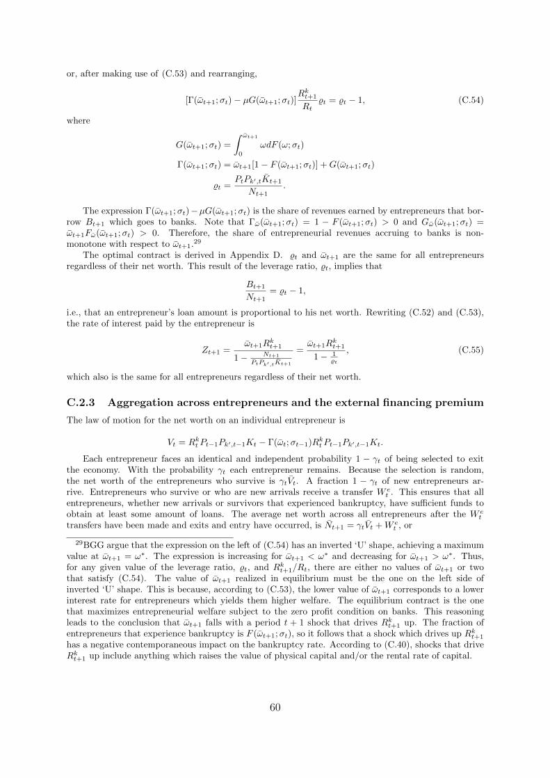
or, after making use of (C.53) and rearranging,

[Γ(ωt+1;σt)− µG(ωt+1;σt)]Rkt+1

Rt%t = %t − 1, (C.54)

where

G(ωt+1;σt) =

∫ ωt+1

0

ωdF (ω;σt)

Γ(ωt+1;σt) = ωt+1[1− F (ωt+1;σt)] +G(ωt+1;σt)

%t =PtPk′,tKt+1

Nt+1.

The expression Γ(ωt+1;σt)−µG(ωt+1;σt) is the share of revenues earned by entrepreneurs that bor-row Bt+1 which goes to banks. Note that Γω(ωt+1;σt) = 1 − F (ωt+1;σt) > 0 and Gω(ωt+1;σt) =ωt+1Fω(ωt+1;σt) > 0. Therefore, the share of entrepreneurial revenues accruing to banks is non-monotone with respect to ωt+1.29

The optimal contract is derived in Appendix D. %t and ωt+1 are the same for all entrepreneursregardless of their net worth. This result of the leverage ratio, %t, implies that

Bt+1

Nt+1= %t − 1,

i.e., that an entrepreneur’s loan amount is proportional to his net worth. Rewriting (C.52) and (C.53),the rate of interest paid by the entrepreneur is

Zt+1 =ωt+1R

kt+1

1− Nt+1

PtPk′,tKt+1

=ωt+1R

kt+1

1− 1%t

, (C.55)

which also is the same for all entrepreneurs regardless of their net worth.

C.2.3 Aggregation across entrepreneurs and the external financing premium

The law of motion for the net worth on an individual entrepreneur is

Vt = Rkt Pt−1Pk′,t−1Kt − Γ(ωt;σt−1)Rkt Pt−1Pk′,t−1Kt.

Each entrepreneur faces an identical and independent probability 1 − γt of being selected to exitthe economy. With the probability γt each entrepreneur remains. Because the selection is random,the net worth of the entrepreneurs who survive is γtVt. A fraction 1 − γt of new entrepreneurs ar-rive. Entrepreneurs who survive or who are new arrivals receive a transfer W e

t . This ensures that allentrepreneurs, whether new arrivals or survivors that experienced bankruptcy, have sufficient funds toobtain at least some amount of loans. The average net worth across all entrepreneurs after the W e

t

transfers have been made and exits and entry have occurred, is Nt+1 = γtVt +W et , or

29BGG argue that the expression on the left of (C.54) has an inverted ‘U’ shape, achieving a maximumvalue at ωt+1 = ω∗. The expression is increasing for ωt+1 < ω∗ and decreasing for ωt+1 > ω∗. Thus,for any given value of the leverage ratio, %t, and Rkt+1/Rt, there are either no values of ωt+1 or twothat satisfy (C.54). The value of ωt+1 realized in equilibrium must be the one on the left side ofinverted ‘U’ shape. This is because, according to (C.53), the lower value of ωt+1 corresponds to a lowerinterest rate for entrepreneurs which yields them higher welfare. The equilibrium contract is the onethat maximizes entrepreneurial welfare subject to the zero profit condition on banks. This reasoningleads to the conclusion that ωt+1 falls with a period t + 1 shock that drives Rkt+1 up. The fraction ofentrepreneurs that experience bankruptcy is F (ωt+1;σt), so it follows that a shock which drives up Rkt+1

has a negative contemporaneous impact on the bankruptcy rate. According to (C.40), shocks that driveRkt+1 up include anything which raises the value of physical capital and/or the rental rate of capital.

60

Nt+1 =γt

{Rkt Pt−1Pk′,t−1Kt −

[Rt−1 +

µ∫ ωt

0ωdF (ω;σt−1)Rkt Pt−1Pk′,t−1Kt

Pt−1Pk′,t−1Kt − Nt

]

× (Pt−1Pk′,t−1Kt − Nt)

}+W e

t . (C.56)

where upper bar over a letter denotes its aggregate average value. Because of its direct effect on en-trepreneurial net worth, γt is referred to as the shock to net worth. For a derivation of the aggregationacross entrepreneurs, see Appendix D.

We now turn to the external financing premium for entrepreneurs. The cost to the entrepreneur ofinternal funds (i.e., his own net worth) is the interest rate Rt which he loses by applying it to capitalrather than buying a risk-free domestic asset. The average payment by all entrepreneurs to the bank isthe entire object in square brackets in (C.56). So, the term involving µ represents the excess of externalfunds over the internal cost of funds. As a result, this is one measure of the financing premium in themodel. Another is Zt+1−Rt, the excess of the interest rate paid by entrepreneurs who are not bankruptover the risk-free rate. This paper calls this the interest rate spread.

Appendix D Model details - not for publication

D.1 Scaling of variables

We adopt the following scaling of variables. The neutral shock to technology is zt and its growth rate isµz,t:

ztzt−1

= µz,t.

The variable Ψt is an investment-specific shock to technology and it is convenient to define thefollowing combination of investment-specific and neutral technology:

z+t = Ψ

α1−αt zt,

µz+,t = µα

1−αΨ,t µz,t. (D.1)

Capital, Kt, and investment, It, are scaled by z+t Ψt. Foreign and domestic inputs into the production

of It (we denote these by Idt and Imt , respectively) are scaled by z+t . Consumption goods (Cmt are imported

intermediate consumption goods, Cdt are domestically produced intermediate consumption goods, and Ctare final consumption goods) are scaled by z+

t . Government expenditure, the real wage and real foreignassets are scaled by z+

t . Exports (Xmt are imported intermediate goods for use in producing exports

and Xt are final export goods) are scaled by z+t . Also, υt is the shadow value in utility terms to the

household of domestic currency and υtPt is the shadow value of one unit of the homogeneous domesticgood. The latter must be multiplied by z+

t to induce stationarity. Pt is the within-sector relative priceof a good. Thus,

kt+1 =Kt+1

z+t Ψt

, kt+1 =Kt+1

z+t Ψt

, idt =Idtz+t

, it =It

z+t Ψt

, itm =Imtz+t

,

cmt =Cmtz+t

, cdt =Cdtz+t

, ct =Ct

z+t

, gt =Gt

z+t

, wt =Wt

z+t Pt

, at :=StA

∗t+1

z+t Pt

,

xmt =Xmt

z+t

, xt =Xt

z+t

, ψz+,t = υtPtz+t , (yt =)yt =

Yt

z+t

, pt =PtPt,

nt+1 =Nt+1

z+t Pt

, we =W et

z+t Pt

.

61

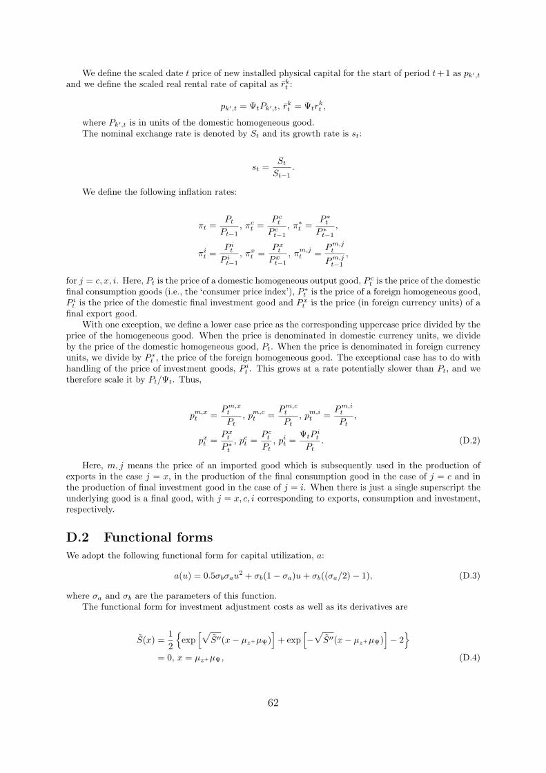
We define the scaled date t price of new installed physical capital for the start of period t+ 1 as pk′,tand we define the scaled real rental rate of capital as rkt :

pk′,t = ΨtPk′,t, rkt = Ψtr

kt ,

where Pk′,t is in units of the domestic homogeneous good.The nominal exchange rate is denoted by St and its growth rate is st:

st =StSt−1

.

We define the following inflation rates:

πt =PtPt−1

, πct =P ctP ct−1

, π∗t =P ∗tP ∗t−1

,

πit =P itP it−1

, πxt =P xtP xt−1

, πm,jt =Pm,jt

Pm,jt−1

,

for j = c, x, i. Here, Pt is the price of a domestic homogeneous output good, P ct is the price of the domesticfinal consumption goods (i.e., the ‘consumer price index’), P ∗t is the price of a foreign homogeneous good,P it is the price of the domestic final investment good and P xt is the price (in foreign currency units) of afinal export good.

With one exception, we define a lower case price as the corresponding uppercase price divided by theprice of the homogeneous good. When the price is denominated in domestic currency units, we divideby the price of the domestic homogeneous good, Pt. When the price is denominated in foreign currencyunits, we divide by P ∗t , the price of the foreign homogeneous good. The exceptional case has to do withhandling of the price of investment goods, P it . This grows at a rate potentially slower than Pt, and wetherefore scale it by Pt/Ψt. Thus,

pm,xt =Pm,xt

Pt, pm,ct =

Pm,ct

Pt, pm,it =

Pm,it

Pt,

pxt =P xtP ∗t

, pct =P ctPt, pit =

ΨtPit

Pt. (D.2)

Here, m, j means the price of an imported good which is subsequently used in the production ofexports in the case j = x, in the production of the final consumption good in the case of j = c and inthe production of final investment good in the case of j = i. When there is just a single superscript theunderlying good is a final good, with j = x, c, i corresponding to exports, consumption and investment,respectively.

D.2 Functional forms

We adopt the following functional form for capital utilization, a:

a(u) = 0.5σbσau2 + σb(1− σa)u+ σb((σa/2)− 1), (D.3)

where σa and σb are the parameters of this function.The functional form for investment adjustment costs as well as its derivatives are

S(x) =1

2

{exp

[√S′′(x− µz+µΨ)

]+ exp

[−√S′′(x− µz+µΨ)

]− 2}

= 0, x = µz+µΨ, (D.4)

62

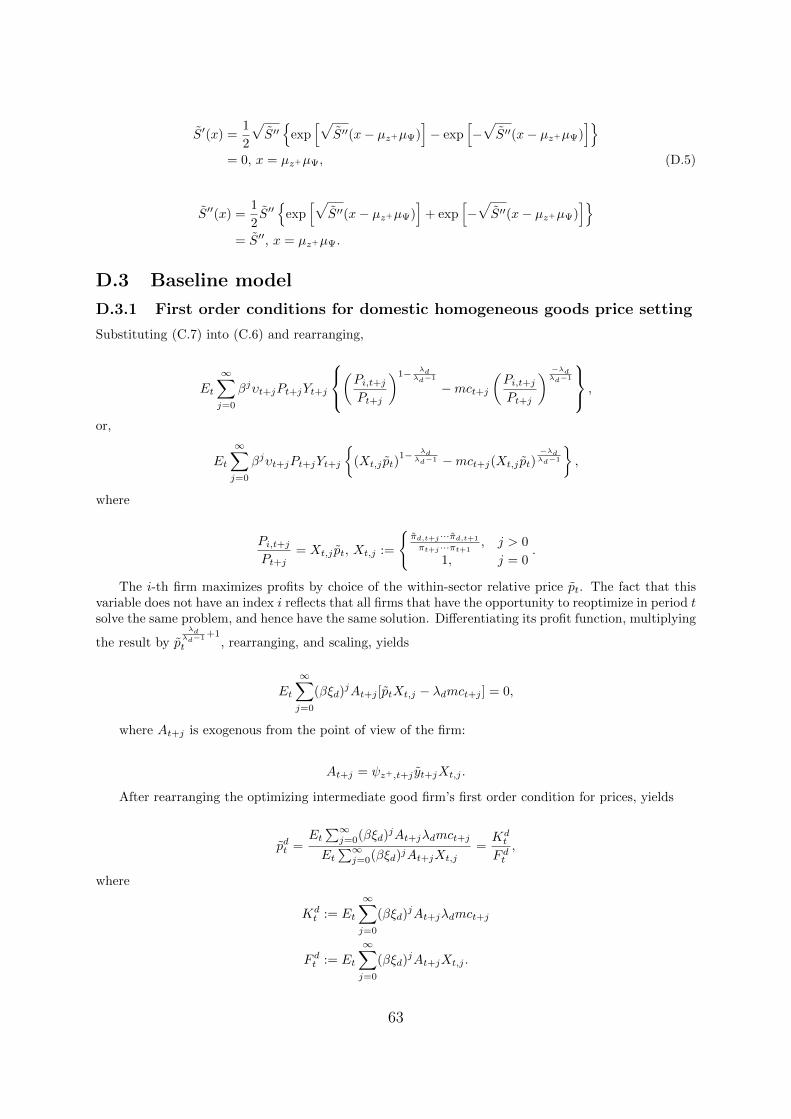
S′(x) =1

2

√S′′{

exp[√

S′′(x− µz+µΨ)]− exp

[−√S′′(x− µz+µΨ)

]}= 0, x = µz+µΨ, (D.5)

S′′(x) =1

2S′′{

exp[√

S′′(x− µz+µΨ)]

+ exp[−√S′′(x− µz+µΨ)

]}= S′′, x = µz+µΨ.

D.3 Baseline model

D.3.1 First order conditions for domestic homogeneous goods price setting

Substituting (C.7) into (C.6) and rearranging,

Et

∞∑j=0

βjυt+jPt+jYt+j

(Pi,t+jPt+j

)1− λdλd−1

−mct+j(Pi,t+jPt+j

) −λdλd−1

,

or,

Et

∞∑j=0

βjυt+jPt+jYt+j

{(Xt,j pt)

1− λdλd−1 −mct+j(Xt,j pt)

−λdλd−1

},

where

Pi,t+jPt+j

= Xt,j pt, Xt,j :=

{πd,t+j ···πd,t+1

πt+j ···πt+1, j > 0

1, j = 0.

The i-th firm maximizes profits by choice of the within-sector relative price pt. The fact that thisvariable does not have an index i reflects that all firms that have the opportunity to reoptimize in period tsolve the same problem, and hence have the same solution. Differentiating its profit function, multiplying

the result by pλdλd−1 +1

t , rearranging, and scaling, yields

Et

∞∑j=0

(βξd)jAt+j [ptXt,j − λdmct+j ] = 0,

where At+j is exogenous from the point of view of the firm:

At+j = ψz+,t+j yt+jXt,j .

After rearranging the optimizing intermediate good firm’s first order condition for prices, yields

pdt =Et∑∞j=0(βξd)

jAt+jλdmct+j

Et∑∞j=0(βξd)jAt+jXt,j

=Kdt

F dt,

where

Kdt := Et

∞∑j=0

(βξd)jAt+jλdmct+j

F dt := Et

∞∑j=0

(βξd)jAt+jXt,j .

63

These objects have the following convenient recursive representations

Et

[ψz+,tyt +

(πd,t+1

πt+1

) 11−λd

βξdFdt+1 − F dt

]= 0

Et

λdψz+,tytmct + βξd

(πd,t+1

πt+1

) λd1−λd

Kdt+1 −Kd

t

= 0.

Turning to the aggregate price index:

Pt =

[∫ 1

0

P1

1−λdit di

]1−λd

=

[(1− ξp)P

11−λdt + ξp(πd,tPt−1)

11−λd

]1−λd(D.6)

After dividing by Pt and rearranging

1− ξd(πd,tπt

) 11−λd

1− ξd= (pdt )

11−λd . (D.7)

In sum, the equilibrium conditions associated with price setting for producers of the domestic ho-mogeneous good are30

Et

[ψz+,tyt +

(πd,t+1

πt+1

) 11−λd

βξdFdt+1 − F dt

]= 0 (D.8)

Et

λdψz+,tytmct + βξd

(πd,t+1

πt+1

) λd1−λd

Kdt+1 −Kd

t

= 0 (D.9)

pt =

(1− ξd)

1− ξd(πd,tπt

) 11−λd

1− ξd

λd

+ ξd

(πd,tπt

pt−1

) λd1−λd

1−λdλd

(D.10)

1− ξd(πd,tπt

) 11−λd

1− ξd

1−λd

=Kdt

F dt(D.11)

πd,t := (πt−1)κd(πct )1−κd−κd(π)κd (D.12)

30After linearizing about the steady state and setting κd = 0,

π − ˆπct =β

1 + κdβEt(πt+1 − ˆπct+1) +

κd1 + κdβ

(πt−1 − ˆπct )

− κdβ(1− ρπ)

1 + κdβˆπct

+1

1 + κdβ

(1− βξd)(1− ξd)ξd

mct,

where a hat indicates log-deviation from steady state.

64

D.3.2 Export demand

Scaling (C.17), yields

xt = (pxt )−ηf y∗t (D.13)

D.3.3 FOCs for export goods price setting

Et

[ψz+,tqtp

ctpxt xt +

(πxt+1

πxt+1

) 11−λx

βξxFx,t+1 − Fx,t

]= 0 (D.14)

Et

[λxψz+,tqtp

ctpxt xtmc

xt + βξx

(πxt+1

πxt+1

) λx1−λx

Kx,t+1 −Kx,t

]= 0 (D.15)

pxt =

(1− ξx)

1− ξx(πxtπxt

)1

1−λx

1− ξx

λx

+ ξx

(πxtπxtpxt−1

) λx1−λx

1−λxλx

(D.16)

1− ξx(πxtπxt

) 11−λx

1− ξx

1−λx

=Kx,t

Fx,t(D.17)

When linearized around steady state and κm,j = 0, eq. (D.14)-(D.17) reduce to

πxt =β

1 + κxβEtπ

xt+1 +

κx1 + κxβ

πxt−1

+1

1 + κxβ

(1− βξx)(1− ξx)

ξxmc

xt

where a hat over a variable indicates log-deviation from steady state.

D.3.4 Demand for domestic inputs in export production

Integrating (C.24),

∫ 1

0

Xdi,tdi =

(λ

τxt Rxt Pt

)ηx(1− ωx)

∫ 1

0

Xi,tdi

=

(λ

τxt Rxt Pt

)ηx(1− ωx)Xt

∫ 1

0(P xi,t)

−λxλx−1 di

(P xt )−λxλx−1

(D.18)

Define P xt , a linear homogeneous function of P xi,t:

P xt =

[∫ 1

0

(P xi,t)−λxλx−1 di

]λx−1−λx

.

Then (P xt

) −λxλx−1

=

∫ 1

0

(P xi,t)−λxλx−1 di

65

and ∫ 1

0

Xdi,tdi =

(λ

τxt Rxt Pt

)ηx(1− ωx)Xt(p

xt )−λxλx−1 (D.19)

where

pxt :=P xtP xt

and the law of motion of pxt is given in (D.16).We now simplify (D.19). Rewriting the second equality in (C.20), yields

λ

Ptτxt Rxt

=StP

xt

Ptqtpctpxt


] 11−ηx

or

λ

Ptτxt Rxt

=StP

xt

PtStP∗tP ct

P ctPt

PxtP∗t


] 11−ηx

or

λ

Ptτxt Rxt

=[ωx(pm,xt )1−ηx + (1− ωx)

] 11−ηx .

Substituting into (D.19),

Xdt =

∫ 1

0

Xdi,tdi =



−λxλx−1 (pxt )−ηxY ∗t

D.3.5 Demand for imported inputs in export production

Scaling (C.26), yields

xmt = ωx

[ωx(pm,xt )1−ηx + (1− ωx)] 1

1−ηx

pm,xt

ηx

(pxt )−λxλx−1 (pxt )−ηf y∗t (D.20)

D.3.6 Value of imports of the intermediate consumption goods producers

It is of interest to have a measure of the value of imports of the intermediate consumption good producers:

StP∗t R

ν,∗t

∫ 1

0

Cmi,tdi.

In order to relate this to Cmt , substitute the demand curve into the previous expression:

StP∗t R

ν,∗t

∫ 1

0

Cmt

(Pm,ct

Pm,ci,t

) λm,cλm,c−1

di = StP∗t R

ν,∗t Cmt (Pm,ct )

λm,cλm,c−1

∫ 1

0

(Pm,ci,t )−λm,cλm,c−1 di

= StP∗t R

ν,∗t Cmt

(Pm,ct

Pm,ct

) λm,c1−λm,c

,

66

where

Pm,ct =

[∫ 1

0

(Pm,ci,t )λm,c

1−λm,c

] 1−λm,cλm,c

.

Thus the total value of imports accounted for by the consumption sector is

StP∗t R

ν,∗t Cmt (pm,ct )

λm,c1−λm,c (D.21)

where

pm,ct =Pm,ct

Pm,ct

.

The derivation for the value of imports used by the investment and export production sectors areanalogous.

D.3.7 Marginal costs of importers

Real marginal cost is

mcm,jt = τm,jt

StP∗t

Pm,jt

Rν,∗t = τm,jt

StP∗t P

ct Pt

P ct Pm,jt Pt

Rν,∗t

= τm,jt

qtpct

pm,jt

Rν,∗t (D.22)

for j = c, i, x.

D.3.8 FOCs for import goods price setting

Et

ψz+,tpm,jt Ξjt +

(πm,jt+1

πm,jt+1

) 11−λm,j

βξm,jFm,j,t+1 − Fm,j,t

= 0 (D.23)

Et

λm,jψz+,tpm,jt mcm,jt Ξjt + βξm,j

(πm,jt+1

πm,jt+1

) λm,j1−λm,j

Km,j,t+1 −Km,j,t

= 0 (D.24)

pm,jt =

(1− ξm,j)

1− ξm,j(πm,jt

πm,jt

) 11−λm,j

1− ξm,j

λm,j

+ ξm,j

(πm,jt

πm,jt

pm,jt−1

) λm,j1−λm,j

1−λm,jλm,j

(D.25)

1− ξm,j(πm,jt

πm,jt

) 11−λm,j

1− ξm,j

1−λm,j

=Km,j,t

Fm,j,t(D.26)

67

for j = c, t, x,31 and where

Ξjt =

cmt j = cxmt j = ximt j = i

.

D.3.9 Wage setting conditions in baseline model

Substituting (C.37) into the objective function, (C.36),

Ejt

∞∑0

(βξw)i[−ζht+iAL

((Wtπw,t+i···πw,t+1

Wt+i

) λw1−λw

Ht+i

)1+σL

1 + σL

+ υt+iWtπw,t+i · · · πw,t+1

(Wtπw,t+i · · · πw,t+1

Wt+i

) λw1−λw

Ht+i1− τy

1 + τw

]Given the rescaled variables,

Wtπw,t+i · · · πw,t+1

Wt+i=Wtπw,t+1 · · · πw,t+1

wt+iz+t+iPt+i

=Wt

wt+iz+t Pt

Xt,i

=Wt

(Wt/Wt

)wt+iz

+t Pt

Xt,i =wt

(Wt/Wt

)wt+i

Xt,i =wtwtwt+i

Xt,i,

where

Xt,i =

{πw,t+i···πw,t+1

πt+iπt+i−1···πt+1µz+,t+i···µz+,t+1, i > 0

1, i = 0.

It is interesting to investigate the value of Xt,i in steady state, as i→∞. Thus,

Xt,i =(πct · · ·πct+i−1)κw(πct+1 · · · πct+i)1−κw−κw(πi)κw(µiz+)ϑw

πt+iπt+i−1 · · ·πt+1µz+,t+i · · ·µz+,t+1

In steady state,

Xt,i =(πi)κw(πi)1−κw−κw(πi)κw(µiz+)ϑw

πiµiz+

=

(πi

πi

)κw(µiz+)ϑw−1

→ 0

31When linearized around steady state and κm,j = 0,

πm,jt − ˆπct =β

1 + κm,jβEt

(πm,jt+1 − ˆπct+1

)+

κm,j1 + κm,jβ

(πm,jt−1 − ˆπct

)− κm,jβ(1− ρπ)

1 + κm,jβˆπct

+1

1 + κm,jβ

(1− βξm,j)(1− ξm,j)ξm,j

mcm,jt .

68

in the no-indexing case, when π = 1, κw = 1 and ϑw = 0.Simplifying using the scaling notation,

Ejt

∞∑i=0


((wtwtwt+i

Xt,i

) λw1−λw

Ht+i

)1+σL

1 + σL

+ υt+iWt+iwtwtwt+i

Xt,i

(wtwtwt+i

Xt,i

) λw1−λw

Ht+i1− τy

1 + τw

]or

Ejt

∞∑i=0


((wtwtwt+i

Xt,i

) λw1−λw

Ht+i

)1+σL

1 + σL

+ ψz+,t+iwtwtXt,i

(wtwtwt+i

Xt,i

) λw1−λw

Ht+i1− τy

1 + τw

]or

Ejt

∞∑i=0


((wtwt+i

Xt,i

) λw1−λw

Ht+i

)1+σL

1 + σLw

λw1−λw (1+σL)

t

+ ψz+,t+iw1+ λw

1−λwt wtXt,i

(wtwt+i

Xt,i

) λw1−λw

Ht+i1− τy

1 + τw

]Differentiating with respect to wt and solving for the wage rate [skipped some math]

w1−λw(1+σL)

1−λwt =

Ejt∑∞i=0(βξw)iζht+iAL

((wtwt+i

Xt,i

) λw1−λw

Ht+i

)1+σL

Ejt∑∞i=0(βξw)i

ψz+,t+iλw

wtXt,i

(wtwt+i

Xt,i

) λw1−λw

Ht+i1−τy1+τw

=ALKw,t

wtFw,t

where

Kw,t := Ejt

∞∑i=0

(βξw)iζht+i

((wtwt+i

Xt,i

) λw1−λw

Ht+i

)1+σL

Fw,t := Ejt

∞∑i=0

(βξw)iψz+,t+i

λwXt,i

(wtwt+i

Xt,i

) λw1−λw

Ht+i1− τy

1 + τw.

Thus, the wage set by reoptimizing households is

wt =

[ALKw,t

wtFw,t

] 1−λw1−λw(1+σL)

.

We now express Kw,t and Fw,t in recursive form [after some skipped math]:

69

Kw,t =ζht H1+σLt + βξwEt

(πw,t+1

πw,t+1

) λw1−λw (1+σL)

Kw,t+1

where

πw,t+1 =Wt+1

Wt=wt+1z

+t+1Pt+1

wtz+t Pt

=wt+1µz+,t+1πt+1

wt(D.27)

Also [after some skipped math],

Fw,t =ψz+,t

λwHt

1− τy

1 + τw+ βξwEt

(wt+1

wt

)(πw,t+1

πw,t+1

)1+ λw1−λw

Fw,t+1.

The second restriction on wt is obtained using the relation between the aggregate wage rate and thewage rates of individual households:

Wt =

[(1− ξw)

(Wt

) 11−λw

+ ξw(πw,tWt−1)1

1−λw

]1−λw.

Dividing both sides by Wt and rearranging,

wt =

1− ξw(πw,tπw,t

) 11−λw

1− ξw

1−λw

Substituting out for wt from the household’s FOC for wage optimization,

1

AL

1− ξw(πw,tπw,t

) 11−λw

1− ξw

1−λw(1+σL)

wtFw,t = Kw,t.

We now derive the relationship between aggregate homogeneous hours worked, Ht, and aggregatehousehold hours,

ht :=

∫ 1

0

hj,tdj.

Substituting the demand for hj,t into the latter expression,

ht =

∫ 1

0

(Wj,t

Wt

) λw1−λw

Htdj

=Ht

(Wt)λw

1−λw

∫ 1

0

(Wj,t)λw

1−λw dj

= wλw

1−λwt Ht, (D.28)

where

wt =Wt

Wt, Wt =

[∫ 1

0

(Wj,t)λw

1−λw dj

] 1−λwλw

70

and

Wt =

[(1− ξw)

(Wt

) λw1−λw

+ ξw

(πw,tWt−1

) λw1−λw

] 1−λwλw

,

so that

wt =

[(1− ξw)(wt)

λw1−λw + ξw

(πw,tπw,t

wt−1

) λw1−λw

] 1−λwλw

=

(1− ξw)

1− ξw(πw,tπw,t

) 11−λw

1− ξw

λw

+ ξw

(πw,tπw,t

wt−1

) λw1−λw

1−λwλw

. (D.29)

In addition to (D.29), we have the following equilibrium conditions associated with sticky wages:

Fw,t =ψz+,t

λww−λw1−λwt ht

1− τy

1 + τw+ βξwEt

(wt+1

wt

)(πw,t+1

πw,t+1

)1+ λw1−λw

Fw,t+1 (D.30)

Kw,t = ζht

(w−λw1−λwt ht

)1+σL

+ βξwEt

(πw,t+1

πw,t+1

) λw1−λw (1+σL)

Kw,t+1 (D.31)

1

AL

1− ξw(πw,tπw,t

) 11−λw

1− ξw

1−λw(1+σL)

wtFw,t = Kw,t. (D.32)

D.3.10 Scaling law of motion of capital

Using (C.38), the law of motion of capital in scaled terms is

kt+1 =1− δ

µz+,tµΨ,tkt + Υt

(1− S

(µz+,tµΨ,tit

it−1

))it. (D.33)

D.3.11 Output and aggregate factors of production

Below we derive a relationship between total output of the domestic homogeneous good, Yt, and aggregatefactors of production.

Consider the unweighted average of the intermediate goods:

Y sumt =

∫ 1

0

Yi,tdi

=

∫ 1

0

[(ztHi,t)

1−αεtKαi,t − z+

t φ]di

=

∫ 1

0

[z1−αt εt

(Ki,t

Hi,t

)αHi,t − z+

t φ

]di

= z1−αt εt

(Kt

Ht

)α ∫ 1

0

Hi,tdi− z+t φ,

71

where Kt is the economy-wide average stock of capital services and Ht is the economy-wide average ofhomogeneous labor. The last expression exploits the fact that all intermediate good firms confront thesame factor prices, and so they adopt the same capital services to homogeneous labor ratio. This followsfrom cost minimization, and holds for all firms, regardless whether or not they have an opportunity toreoptimize. Then,

Y sumt = z1−αt εtK

αt H

1−αt − z+

t φ.

Recall that the demand for Yj,t is

(PtPi,t

) λdλd−1

=Yi,tYt

,

so that

Yt :=

∫ 1

0

Yi,tdi =

∫ 1

0

Yt

(PtPi,t

) λdλd−1

di = YtPλdλd−1

t

(Pt

) λd1−λd ,

where

Pt =

[∫ 1

0

Pλd

1−λdi,t di

] 1−λdλd

. (D.34)

Dividing by Pt,

pt =

∫ 1

0

(PitPt

) λd1−λd

di

1−λdλd

,

or,

pt =

(1− ξp)

1− ξp(πd,tπt

) 11−λd

1− ξp

λd

+ ξp

(πd,tπt

pt−1

) λd1−λd

1−λdλd

. (D.35)

The preceding implies

Yt = (pt)λdλd−1 Yt = (pt)

λdλd−1

[z1−αt εtK

αt H

1−αt − z+

t φ],

or, after scaling by z+t ,

yt = (pt)λdλd−1

[εt

(1

µΨ,tµz+,tkt

)αH1−αt − φ

],

where

kt = ktut. (D.36)

Plugging Ht from (D.28),

yt = (pt)λdλd−1

[εt

(1

µΨ,tµz+,tkt

)α(w

λw1−λwt ht

)1−α

− φ

].

72

D.3.12 Restrictions across inflation rates

We now consider the restrictions across inflation rates implied by the relative price formulas. In termsof the expressions in (D.2), there are the restrictions implied by Pm,jt /pm,jt−1, j = x, c, i, and pxt . Therestrictions implied by the other two relative prices in (D.2), pit and pct , have already been used in (C.16)and (D.33), respectively. Finally, we also use the restriction across inflation rates implied by qt/qt−1 and(C.23). Thus,

pm,xt

pm,xt−1

=πm,xt

πt(D.37)

pm,ct

pm,ct−1

=πm,ct

πt(D.38)

pm,it

pm,it−1

=πm,it

πt(D.39)

pxtpxt−1

=πxtπ∗t

(D.40)

qtqt−1

=stπ∗t

πct. (D.41)

D.3.13 Endogenous variables of the baseline model

In above we derived the following 70 equations:(C.3), (C.4), (C.5), (D.8), (D.9), (D.10), (D.11), (D.12), (D.3), (C.10), (C.11), (C.12), (C.15), (C.16),

(C.14), (D.13), (C.21), (C.20), (C.27), (D.14), (D.15), (D.16), (D.17), (D.20), (C.29), (D.23), (D.24),(D.25), (D.26), (C.32), (D.22), (D.4), (D.5), (D.33), (C.39), (C.41), (C.42), (C.43), (C.44), (C.45), (C.47),(D.30), (D.31), (D.32), (D.29), (C.35), (D.27), (D.28), (D.36), (C.49), (C.51), (C.50), (D.37), (D.38),(D.39), (D.40), (D.41), (C.48),

which can be used to solve for the following 70 unknowns:rkt , wt, R

ν,∗t , Rft , Rxt , Rt, mct, mc

xt , mcm,ct , mcm,it , mcm,xt , πt, π

xt , πct , π

it, π

m,ct , πm,it , πm,xt , pct , p

xt ,

pit, pm,xt , pm,ct , pm,it , pk′,t, kt+1, kt+1, ut, ht, Ht, qt, it, ct, xt, at, ψz+,t, yt, K

dt , F dt , πd,t, pt,Kx,t, Fx,t,

πxt , pxt , {Km,j,t, Fm,j,t, πm,jt , pm,jt ; j = c, i, x}, Kw,t, Fw,t, π

wt , Rkt , Φt, St, S

′t, a(ut), wt, c

mt , imt , xmt , πw.

D.4 Equilibrium conditions for financial frictions model

D.4.1 Derivation of optimal contract

As noted in the text, it is supposed that the equilibrium debt contract maximizes entrepreneurial welfaresubject to the zero profit condition on banks and the specified required return on household bankliabilities. The date t debt contract specifies a level of debt Bt+1 and a state t + 1-contingent rateof interest, Zt+1. We suppose that entrepreneurial welfare corresponds to the entrepreneur’s expectedwealth at the end of the contract. It is convenient to express welfare as a ratio to the amount theentrepreneur could receive by depositing his net worth in a bank:

Et∫∞ωt+1

[Rkt+1ωPtPk′,tKt+1 − Zt+1Bt+1

]dF (ω;σt)

RtNt+1

=Et∫∞

¯ωt+1[ω − ωt+1]dF (ω;σt)R

kt+1PtPk′,tKt+1

RtNt+1

= Et

{[1− Γ(ωt+1;σt)]

Rkt+1

Rt

}%t,

73

after making use of (C.52), (C.53) and

1 =

∫ ∞0

ωdF (ω;σt) =

∫ ∞ωt+1

ωdF (ω;σt) +G(ωt+1;σt).

We can equivalently characterize the contract by a state-t+ 1 contingent set of values for ωt+1 and avalue of %t. The equilibrium contract is the one involving ωt+1 and %t which maximizes entrepreneurialwelfare (relative to RtNt+1) subject to the bank zero profits condition. The Lagrangian representationof this problem is

max%t,{ωt+1}

Et

{[1− Γ(ωt+1;σt)]

Rkt+1

Rt%t + λt+1

([Γ(ωt+1;σt)− µG(ωt+1;σt)]

Rkt+1

Rt%t − %t + 1

)},

where λt+1 is the Lagrange multiplier which is defined for each period t+ 1 state of nature. The FOCsfor this problem are:

Et

{[1− Γ(ωt+1;σt)]

Rkt+1

Rt+ λt+1

([Γ(ωt+1;σt)− µG(ωt+1;σt)]

Rkt+1

Rt− 1

)}= 0

−Γω(ωt+1;σt)Rkt+1

Rt+ λt+1[Γω(ωt+1;σt)− µGω(ωt+1;σt)]

Rkt+1

Rt= 0


Rt%t − %t + 1 = 0,

where the absence of λt+1 from the complementary slackness condition reflects that it is assumed thatλt+1 > 0 in each period t + 1 state of nature. Substituting out for λt+1 from the second equation intothe first, the FOCs reduce to

Et

[1− Γ(ωt+1;σt+1)]Rkt+1

Rt+ Γω(ωt+1;σt)

Γω(ωt+1;σt)−µGω(ωt+1;σt)×(


Rt− 1)

= 0 (D.42)


Rt%t − %t + 1 = 0 (D.43)

for t = 0, 1, 2, . . . ,∞ and for t = −1, 0, 1, 2, . . . respectively.Since Nt+1 does not appear in the last two equations, %t and ωt+1 are the same for all entrepreneurs

regardless of their net worth.

D.4.2 Derivation of aggregation of across entrepreneurs

Let f(Nt+1) denote the density of entrepreneurs with net worth Nt+1. Then, aggregate average networth, Nt+1, is

Nt+1 =

∫Nt+1

Nt+1f(Nt+1)dNt+1.

We now derive the law of motion of Nt+1. Consider the set of entrepreneurs who in period t− 1 hadnet worth N . Their net worth after they have settled with the bank in period t is denoted V Nt , where

V Nt = Rkt Pt−1Pk′,t−1KNt − Γ(ωt;σt−1)Rkt Pt−1Pk′,t−1K

Nt , (D.44)

where KNt is the amount of physical capital that entrepreneurs with net worth Nt acquired in period

t− 1. Clearing in the market for capital requires:

74

Kt =

∫Nt

KNt f(Nt)dNt.

Multiplying (D.44) by f(Nt) and integrating over all entrepreneurs,

Vt = Rkt Pt−1Pk′,t−1Kt − Γ(ωt;σt−1)Rkt Pt−1Pk′,t−1Kt.

Writing this out more fully:

Vt = Rkt Pt−1Pk′,t−1Kt −{

[1− F (ωt;σt−1)]ωt +

∫ ωt

0

ωdF (ω;σt−1)

}Rkt Pt−1Pk′,t−1Kt

= Rkt Pt−1Pk′,t−1Kt

−{

[1− F (ωt;σt−1)]ωt + (1− µ)

∫ ωt

0

ωdF (ω;σt−1) + µ

∫ ωt

0

ωdF (ω;σt−1)

}Rkt Pt−1Pk′,t−1Kt.

Note that the first two terms in braces correspond to the net revenues of the bank, which must equalRt−1(Pt−1Pk′,t−1Kt − Nt). Substituting

Vt = Rkt Pt−1Pk′,t−1Kt −

{Rt−1 +

µ∫ ωt

0ωdF (ω;σt−1)Rkt Pt−1Pk′,t−1Kt

Pt−1Pk′,t−1Kt − Nt

}(Pt−1Pk′,t−1Kt − Nt)

which implies (C.56) in the main text.

D.4.3 Adjustment to the baseline model when financial frictions are intro-duced

Consider the households. Households no longer accumulate physical capital, and the FOC (C.42) mustbe dropped. No other changes need to be made to the household FOCs. Eq. (C.45) can be interpretedas applying to the household’s decision to make bank deposits. The household eq-ns (D.33) and (C.43)pertaining to the law of motion and FOC for investment respectively, can be thought of as reflecting thatthe household builds and sells physical capital, or it can be interpreted as the FOC of many identicalcompetitive firms that build capital (note that each has a state variable in the form of lagged investment).We must add the three equations pertaining to the entrepreneur’s loan contract: the law of motion of networth, the bank’s zero profit condition and the optimality condition. Finally, we must adjust the resourceconstraints to reflect the resources used in bank monitoring and in consumption by entrepreneurs.

We adopt the following scaling of variables, noting that W et is set so that its scaled counterpart is

constant

nt+1 =Nt+1

Ptz+t

, we =W et

Ptz+t

.

Dividing both sides of (C.56) by Ptz+t , we obtain the scaled law of motion for net worth:

nt+1 =γt

πtµz+,t[Rkt pk′,t−1kt −Rt−1(pk′,t−1kt − nt)− µG(ωt;σt−1)Rkt pk′,t−1kt] + we (D.45)

for t = 0, 1, 2, . . .. Eq. (D.45) has a simple intuitive interpretation. The first object in square bracketsis the average gross return across all entrepreneurs in period t. The two negative terms correspond towhat the entrepreneurs pay to the bank, including the interest paid by non-bankrupt entrepreneurs andthe resources turned over to the bank by the bankrupt entrepreneurs. Since the bank makes zero profits,the payment to the bank by entrepreneurs must equal bank costs. The term involving Rt−1 represents

75

the cost of funds loaned to entrepreneurs by the bank, and the term involving µ represents the bank’stotal expenditures on monitoring costs.

The zero profit condition on banks, (D.43), can be expressed in terms of the scaled variables as

Γ(ωt+1;σt)− µG(ωt+1;σt) =RtRkt+1

(1− nt+1

pk′,tkt+1

)(D.46)

for t = −1, 0, 1, 2, . . .. The optimality condition for bank loans is (D.42).The output equation, (C.49), does not have to be modified. Instead, the resource constraint for

domestic homogeneous goods (C.50) needs to be adjusted for the monitoring costs:

yt − dt =gt + (1− ωc)(pct)ηcct + (pit)ηi

(it + a(ut)

ktµψ,tµz+,t

)(1− ωt)

+[ωx(pm,xt )1−ηx + (1− ωx)


−λxλx−1 (pxt )−ηf y∗t , (D.47)

where

dt =µG(ωt;σt−1)Rkt pk′,t−1kt

πtµz+,t.

When the model is brought to the data, measured GDP is yt adjusted for both monitoring costsand, as in the baseline model, capital utilization costs

gdpt = yt − dt − (pit)ηi

(a(ut)

ktµψ,tµz+,t

)(1− ωi).

Account has to be taken of the consumption by existing entrepreneurs. The net worth of theseentrepreneurs is (1−γt)Vt and it is assumed that a fraction, 1−Θ, is taxed and transferred in lump-sumform to households, while the complementary fraction, Θ, is consumed by the existing entrepreneurs.This consumption can be taken into account by subtracting

Θ1− γtγt

(nt+1 − we)z+t Pt

from the right side of (C.9). In practice we do not make this adjustment because we assume Θ issufficiently small that the adjustment is negligible.

The financial frictions brings a net increase of two equations (we add (D.42), (D.45) and (D.46), anddelete (C.42)) and two variables, nt+1 and ωt+1. This increases the size of our system to 72 equationsin 72 unknowns. The financial frictions also introduce the additional shocks, σt and γt.

D.5 Measurement equations

Below we report the measurement equations we use to link the model to the data. Our data series forinflation and interest rates are annualized in percentage terms, so we make the same transformation forthe model variables, i.e. multiplying by 400:

Rdatat = 400(Rt − 1)− ϑ1400(R− 1)

R∗,datat = 400(R∗t − 1)− ϑ1400(R∗ − 1)

πd,datat = 400 log πt − ϑ1400 log π + εmeπ,t

πc,datat = 400 log πct − ϑ1400 log πc + εmeπc,t

πi,datat = 400 log πit − ϑ1400 log πi + εmeπi,t

π∗,datat = 400 log π∗t − ϑ1400 log π∗,

76

where εmei,t denote the measurement errors for the respective variables. In addition, ϑ1 ∈ {0, 1} allowsus to handle demeaned and non-demeaned data. In particular, the data for interest rates and foreigninflation are not demeaned. The domestic inflation rates are demeaned.

We use undemeaned first differences in total hours worked,

∆ logHdatat = 100∆ logHt + εmeH,t.

We use demeaned first-differenced data for the remaining variables. This implies setting ϑ2 = 1below:

∆ log Y datat = 100

logµz+,t + ∆ log

yt − pita(ut)kt

µψ,tµz+,t− dt −

κ

2

N−1∑j=0

(vjt )2(1−F jt )ljt

− ϑ2100(logµz+) + εmey,t

∆ log Y ∗,datat = 100(logµz+,t + ∆ log y∗t )− ϑ2100(logµz+)

∆ logCdatat = 100(logµz+,t + ∆ log ct)− ϑ2100(logµz+) + εmec,t

∆ logXdatat = 100(logµz+,t + ∆ log xt)− ϑ2100(logµz+) + εmex,t

∆ log qdatat = 100∆ log qt + εmeq,t

∆ logMdatat = 100(logµz+,t + ∆ log Importst)− ϑ2100(logµz+) + εmeM,t

= 100

logµz+,t + ∆ log

cmt (pm,ct )

λm,c1−λm,c

+imt (pm,it )λm,i

1−λm,i

+xmt (pm,xt )λm,x

1−λm,x

− ϑ2100(logµz+) + εmeM,t

∆ log Idatat = 100[logµz+,t + logµψ,t + ∆ log it]− ϑ2100(logµz+ + logµψ) + εmeI,t

∆ logGdatat = 100(logµz+,t + ∆ log gt)− ϑ2100(logµz+) + εmeg,t

Note that neither measured GDP nor measured investment include investment goods used for capitalmaintenance. To calculate measured GDP we also exclude monitoring costs and recruitment costs.

The measurement equation for demeaned first-differenced wages is

∆ log(Wt/Pt)data = 100∆ log

Wt

z+t Pt

= 100(logµz+,t + ∆ log wt)− ϑ2100(logµz+) + εmeW/P,t.

Finally, we measure demeaned first-differenced net worth and interest rate spread as follows:

∆ logNdatat = 100(logµz+,t + ∆ log nt)− ϑ2100(logµz+) + εmeN,t

∆ logSpreaddatat = 100∆ log(zt+1 −Rt) = 100∆ log

(ωt+1R

kt+1

1− nt+1

pk′,tkt+1

−Rt

)+ εmeSpread,t

77

Financial frictions in a DSGE model for Latvia

Documents

Transcript of Financial frictions in a DSGE model for Latvia