Financial Fragmentation And Insider Arbitrage

This Draft: February 2010

Preliminary

Stefan Klonner, Goethe University, Frankfurt

Ashok S. Rai, Williams College

Abstract: If there were no impediments to the �ow of capital across space, then the

returns to capital should be equalized. We provide evidence to the contrary. There are

large di¤erences in the return to comparable investments across di¤erent towns in the state

of Tamil Nadu in South India. We explore why these di¤erences are not arbitraged away

�and suggest that if an insider has monopoly power in arbitraging across towns then it is

in his pro�t-maximizing interest to reduce but not eliminate the di¤erences in returns to

capital.

JEL Codes: O16, G21

Keywords: credit constraints, limits to arbitrage

0We are grateful to the Chit Fund company (in South India) for sharing their data and their time.

And to Zhaoning Wang for research assistance. All errors are our own. Klonner: University of Frankfurt,

stefan@klonner.de; Rai: Dept. of Economics, Williams College, Williamstown, MA 01267, arai@williams.edu

1

1 Introduction

The misallocation of capital is widely thought to contribute underdevelopment and pro-

duction ine¢ ciencies (Banerjee and Du�o, 2005, Hsieh and Klenow, 2009). Recent micro-

evidence has documented the ine¢ cient �ow of capital within developing countries. For

instance, de Mel, Woodru¤ and Mckenzie (2009) and Paulson,Townsend and Karaivanov

(2006) �nd that �nance does not �ow to high return entrepreneurs in Sri Lanka and Thai-

land respectively. Banerjee and Munshi (2004) suggest that �nance does not �ow across

ethnic lines in India.

In this paper we investigate the �ows of capital across space. We �nd large and signif-

icant di¤erences in the returns to comparable �nancial investments across location-speci�c

�nancial markets in a southern Indian state. If �nance �owed to its highest use, such

di¤erences should not exist. The natural question then arises: Why doesn�t arbitrage

�borrowing from locations where �nance is cheap and investing in locations where �nance

is scarce �eliminate these di¤erences? We �nd that evidence of limited arbitrage by an

"insider" and suggest a reason why it is costly for non-insiders enter the arbitrage business.

Imagine for illustrative purposes that there are just two locations, L and H. Several

loan transactions take place in each location. Suppose that the average interest rates are

signi�cantly lower in location L than in locationH, even when controlling for any di¤erences

in the size, term, riskiness, contractual features of the loans between L and H: This suggests

�nancial fragmentation: an ine¢ ciency in the allocation of capital over space. Location H

apparently has higher return projects than location L �and capital should be �owing from

L to H �so as to equalize the average returns. If an arbitrageur were to borrow from L

and invest in H; he would make pro�ts as long as the spread in interest rates was higher

than the costs of arbitrage. Note that a wedge between the borrowing and savings interest

rates will create such a transactions cost of arbitrage.

In the paper, we analyze data from 78 locations in the state of Tamil Nadu in south

India. We use data from a non-bank �nancial intermediary that organizes auctions in

di¤erent locations to intermediate between borrowers and savers in that location. There

2

are two advantages of this dataset. First, interest rate in each location are determined

by auction and so should re�ect local productivity shocks. In contrast, commerical bank

interest rates are determined centrally in India and hence are identical across locations.

Secondly, since loan contracts are standardized and explicit across locations and we can

compare interest rates while adjusting for di¤erences in loan characteristics. In contrast,

the spatial variation in interest rates on informal loans by moneylender observed elsewhere

could have arisen because of unobserved variation in contractual terms or riskiness (Banerjee

and Du�o, 2005):

We �nd evidence of �nancial fragmentation across the 78 locations. Put di¤erently,

the interest rates across locations are signi�cantly and substantially di¤erent from each

other even when controlling for loan characteristics (such as the length and amount of the

loan, the collateral required) and riskiness (as measured by ex-post default rates). The

annual interest rates on savings range from 6:56 percent to 12:63 percent Remarkably,

fragmentation occurs even though the company is engaged in arbitrage across locations.

The company participates in about a third of the loan transactions and systematically

borrows when interest rates are low and saves when they are high. We think of this as a

form of insider arbitrage �and �nd that the company�s behavior suggests that it has an

investment opportunity with higher return than the average of the 78 locations it operates

in. While our model suggests that e¢ ciency would be lower (�nancial fragmentation

greater) in the absence of insider arbitrage, we have cannot test this claim because we have

no data on �nancial fragmentation in the absence of an inside arbitrageur. Finally, we

provide some indirect evidence that the transactions costs associated with intermediation

can explain why there are no outside arbitrageurs. These transaction costs (a) limit the

interest-rate spread between locations and hence prevent �nancial e¢ ciency and (b) allow

the insider to make monopoly pro�ts from the interest-rate spreads.

Our paper forms a bridge, then, between the empirical research on �nancial constraints

in development (cited above) and a literature on the limits to arbitrage in �nancial markets

(Shleifer and Vishny, 1997). While much of the latter literature studies how risk aversion,

3

transaction costs or agency di¢ culties can impede arbitrage, Borenstein et al (2008) explore

a similar market power explanation for price di¤erences despite arbitrage opportunities in

California�s electricity market. In their study, regulatory barriers prevent �rms from

exploiting the arbitrage opportunities. In our paper, there are no regulatory di¤erences

across locations that would prevent arbitrage.

The paper proceeds as follows. In Section 2 we provide background on bidding Roscas

in South India and on our dataset. In Section 3 we outline some of the testable implications

from a simple model. We discuss our results in Section 4:

2 Institutional Background

This study uses data on Rotating Savings and Credit Associations (commonly referred to

as Roscas). Roscas intermediate between borrowers and savers but do so quite di¤erently

from banks (Anderson and Baland, 2003; Besley, Coate and Loury, 1994). In this section

we provide some background on how the Roscas in our study operate. We also describe

the sample of Rosca participants that we will use in our subsequent empirical analysis.

Rules

Roscas are �nancial institutions in which the accumulated savings are rotated among par-

ticipants. Participants in a Rosca meet at regular intervals, contribute into a "pot" and

rotate the accumulated contributions. So there are always as many Rosca members as

meetings. In random Roscas, the pot is allocated by lottery and in bidding Roscas the pot

is allocated by an auction at each meeting. Our study uses data on the latter.

More speci�cally, the bidding Roscas in our sample work as follows. Each month

participants contribute a �xed amount to a pot. They then bid to receive the pot in an

oral ascending bid auction where previous winners are not eligible to bid. The highest

bidder receives the pot of money less the winning bid and the winning bid is distributed

among all the members as an interest dividend. The winning bid can be thought of as the

4

price of capital. Consequently, higher winning bids mean higher interest payments. Over

time, the winning bid falls as the duration for which the loan is taken diminishes. In the

last month, there is no auction as only one Rosca participant is eligible to receive the pot.

We illustrate the rules with a numerical example:

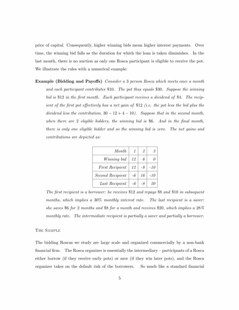
Example (Bidding and Payo¤s) Consider a 3 person Rosca which meets once a month

and each participant contributes $10: The pot thus equals $30. Suppose the winning

bid is $12 in the �rst month. Each participant receives a dividend of $4: The recip-

ient of the �rst pot e¤ectively has a net gain of $12 (i.e. the pot less the bid plus the

dividend less the contribution, 30� 12 + 4� 10). Suppose that in the second month,

when there are 2 eligible bidders, the winning bid is $6: And in the �nal month,

there is only one eligible bidder and so the winning bid is zero: The net gains and

contributions are depicted as:

Month 1 2 3

Winning bid 12 6 0

First Recipient 12 -8 -10

Second Recipient -6 16 -10

Last Recipient -6 -8 20

The �rst recipient is a borrower: he receives $12 and repays $8 and $10 in subsequent

months, which implies a 30% monthly interest rate. The last recipient is a saver:

she saves $6 for 2 months and $8 for a month and receives $20, which implies a 28%

monthly rate. The intermediate recipient is partially a saver and partially a borrower.

The Sample

The bidding Roscas we study are large scale and organized commercially by a non-bank

�nancial �rm. The Rosca organizer is essentially the intermediary �participants of a Rosca

either borrow (if they receive early pots) or save (if they win later pots), and the Rosca

organizer takes on the default risk of the borrowers. So much like a standard �nancial

5

intermediary, the Rosca organizer screens borrowers and secures loan repayments, so that

savers are assured of receiving funds in later rounds.

The data we use is from the internal records of an established Rosca organizer in the

southern Indian state of Tamil Nadu.1 Our sample comprises Roscas that started on

or after January 1, 2002 and ended by November 2005: These Roscas took place in 78

branches of a non-bank �nancial �rm. Our sample comprises 2056 Roscas of 34 di¤erent

durations and contributions. The most common Rosca denomination had 25 participants

and a Rs. 400 monthly contribution (with a total pot of Rs. 10; 000). There were also

Roscas that met for longer durations (30 or 40 months) and with higher and lower monthly

contributions. The average duration of the Rosca in our sample was 29:55 months. These

di¤erent Rosca denominations serve to match borrowers and savers with di¤erent investment

horizons. Descriptive statistics of the Rosca denominations are in Table 1. Descriptive

statistics at the Rosca level are in Table 2.

For each Rosca in our sample, we compute the savings interest rate r as the solution to

T�1Xi=1

(�m+ divi)(1 + r)T�i + (Tm� c) = 0 (1)

where m is the individual monthly contribution, divt is the dividend in month t paid to

each participant, T is the number of rounds/months/participants, and c is commission to

the organizer in each round. The commission c is usually �xed at �ve percent of the value

of the pot, i.e. c = 0:05mT . According to the rules of these Roscas, div1 = divT = 0.

Moreover, for all t = 2; :::; T � 1, the dividend is:

divt =bt � cT

;

where bt is the winning bid in the round-t auction. Notice that the minimum winning bid

for t = 2; :::; T � 1 is c. If none of the Rosca participants is willing to bid more than c in a1Bidding Roscas are a signi�cant source of �nance in South India, where they are called chit funds.

Deposits in regulated bidding Roscas were 12:5% of bank credit in the state of Tamil Nadu and 25% of bank

credit in the state of Kerala in the 1990s, and have been growing rapidly (Eeckhout and Munshi, 2004).

There is also a substantial unregulated chit fund sector.

6

given auction, the round t recipient of the pot is determined through a lottery among the

eligible Rosca participants of that round. She receives the pot at a discount of precisely c.

The savers (last-round winners) in these Roscas are insured against winners of earlier

pots failing to make contributions by the organizer. Rather than asking for physical

collateral, the organizer requires auction winners to provide cosigners before releasing the

loans. Cosigners are required to be salaried employees with a minimum monthly income

that depends on the Rosca denomination. This is because the organizer has a legally

enforceable claim against their future income as collateral for the loan. The organizer may

also verify the auction winner�s income before releasing the loan. For instance, a self-

employed person will be asked for tax returns or bank statements while a salaried employee

will be asked for an earning record. Veri�cation is a form of costly screening because it

takes time and e¤ort.

The only risk that the saver faces therefore is the risk that the organizer itself may go

bankrupt before the Rosca ends. This is indeed a real risk in the Indian context (where

numerous chit fund companies have folded), but it is common to all the savers in all the 78

branches in the sample.

The average annual interest rate for a saver in these Rosca is 9.17 percent per year with

a standard deviation of 1.18 percent. At each location, interest rates are determined locally

through auctions. In contrast, the commercial bank savings rates are determined centrally

and are not based on local supply and demand for credit. So there is no variation. We

have obtained the rates on 3-6 month �xed deposits from the ICICI Bank, a large and well-

networked commercial bank, and those rates were at 6 percent or below for all of the study

period (2002-2005) with the exception of a six month period starting April 2002 when the

rate was 7.75 percent. The interest rates on commercial bank savings are substantially lower

than in the organized Rosca sector. This could re�ect a risk premium that the Rosca saver

must pay (since the organizer of the Roscas is more likely to go bankrupt than ICICI bank).

In addition, there is a uncertainty with the realized interest rate for a Rosca participant

(depending on the composition of the Rosca) that is absent in the commercial bank �xed

7

deposits.

"The Company"

In what follows we shall pay special attention to a particular investor who behaves quite

di¤erently from other Rosca participants. This investor operates in all 78 branches, and

takes several postions in Roscas in each branch. Further, this investor is not considered a

default risk by the Rosca organizer and so does not have to provide cosigners as collateral.

Field conversations and observations indicate that this investor has close business ties to

the Rosca organizer; for that reason it is not charged a commission for participation.

Other participants, by contrast, are location-speci�c, are charged a commission, and need

to provide cosigners when they win early pots. We shall interpret this investor as an

insider and use the term "the company" to refer to the single entity that comprises this

investor and the Rosca organizer in what follows.

3 A Model of Arbitrage in Roscas

In this section we consider a simple model of arbitrage between Roscas in two locations.

Our aim is to clarify how arbitrage can reduce reduce �nancial ine¢ ciencies but also to

point out the incompleteness of such arbitrage when there are barriers to entry.

Consider two spatially separated locations, each with n private agents. Each agent is

endowed with a dollar in the �rst period. Each agent has an investment opportunity with

a �xed investment cost of 2 at date 1 and yield 2p at date 2: Agents do not discount the

future. Agents vary in their productivity p. In each location, agents�types are distributed

according to Fi. For analytical convenience, we assume that each of the density functions

f1 and f2 is symmetric. Denote the corresponding mean and median by �i. Without loss

of generality, we assume �1 > �2, i.e. agents in location 1 are on average more productive

than in location 2. The aggregate cumulative distribution function of types will be denoted

by F , where F (p) = 12 (F1(p) + F2(p)) : The mean of the aggregate distribution of types is

8

� = (�1 + �2)=2 and its median will be denoted by m: We assume private information on

individual types, i.e. each agent observes only her own type and knows the distribution of

types in her location.

In parts of the subsequent analysis, we employ the following additional assumptions:

A1 Fi is unimodal

A2 F2 is a translation of F1, i.e. F2(p) = F1(p+ �1 � �2)

We model simple Roscas with two participants and hence two rounds. There is an

auction only at date 1: Each Rosca participant contributes a dollar at date 1 and the

auction is for the repayment amount b that is due at date 2: The winner of the auction

receives the pot and invests. There is a �xed commission of c charged for any net transfer

in a Rosca. As there are two net transfers in a Rosca, one in the �rst and one in the

second period, the total commission is 2c: We assume that each of the two participants

pays a commission of c when the Rosca is over (for simplicity, c is not part of the winning

bid). So at date 2; the winner pays b to the loser of the �rst-round auction and c to the

organizer. The loser of the �rst-round auction receives b from the winner and also pays c

to the organizer. Consequently, the interest rate on the auction loser�s saving of $1 in the

Rosca is b� 1� c while the winner of the date 1 auction borrows at a rate of b� 1+ c. The

di¤erence between the borrowing and savings rate is 2c. In this way, by slightly abstracting

from the the speci�c rules that are used in practice in the Roscas in our sample, our model

allows to relate the winning bid directly to the implied interest rates. In addition, the

solution of the model is greatly simpli�ed. Modelling two persons according to the actual

rules of our sample Roscas gives identical qualitative results.

No Arbitrage

We �rst show that, in the absence of arbitrage, the interest rate di¤erence across locations is

given by di¤erences in average productivity, �1��2. More formally, an agent�s willingness

9

to pay for the date 1 pot is found by equalizing her payo¤ from winning, 2p� b� c; to her

payo¤ from losing, b� c; which gives

b� = p:

In a Rosca, two individuals of a location are randomly matched. In each Rosca, each

participant is uninformed about the other participant�s type, and hence willingness to pay.

We are thus in a situation of a symmetric, independent, private-value auction. Since the

Roscas we consider have open-ascending bid auctions, the appropriate bidding equilibrium

is most easily found by modelling the auction as a second-price sealed bid auction, which

is payo¤-equivalent. It can be shown that, in such an auction, each bidder determines her

bid by a strictly increasing function hi(p), where hi(p) � p for all p, hence there is some

overbidding relative to one�s valuation of the pot. Denoting by Pi;k:2 the k�th highest order

statistic of a sample of size two drawn from Fi, the di¤erence in interest rates between

branches, or spread for short, is

�r = E[h1(P2:2)� h2(P2:2)]:

Under assumption A2, we have that h2(p) = h1(p)� (�1��2): Denoting �1��2 by �� we

then have that

�r = ��:

When the e¢ ciency of allocations is concerned, the best possible outcome in this scenario

is that, in location i, all projects with a date 2 payo¤ greater than mi are �nanced (i = 1; 2).

E¢ ciency, on the other hand, implies that all projects with a date 2 payo¤ greater than

m are �nanced in each of the two locations. It follows immediately that the aggregate

allocation of capital will be ine¢ cient if �� > 0:

Example with Uniform Distributions We consider uniform speci�cations of F1 and

F2 with an identical range of �,

Fi(b) =(b� �i)�

+1

2; �i �

�

2� b � �i +

�

2:

10

We will assume that the two distributions overlap su¢ ciently, speci�cally

�1 � �2 � �:

When all above-median projects are �nanced in each location, the aggregate payo¤

at date 2 is

�a =��1 + �2 +

�

2

�n

because, in location i, the average payo¤ per doller invested is E[PijPi � mi] =

�i+�=4. A fully e¢ cient allocation of capital, on the other hand, implies an aggregate

payo¤ of

�� =n

�

h��1 + �+

�

2

���1 � �+

�

2

�+��+ �2 +

�

2

���2 � �+

�

2

�i;

where � = (�1 + �2)=2. Notice that2n�

��i � �+ �

2

�dollars are invested in location i

while the respective mean payo¤ is 12��+ (�i +

�2 )�per dollar invested. The amount

which has to be moved from location 2 to location 1 to achieve an e¢ cient allocation

of capital, is

T � =���n:

It can be shown, moreover, that each dollar which is moved from 2 to 1 earns an extra

return of ��=2 on average. The expected welfare di¤erenc between a fully e¢ ciencient

allocation of capital and autarky thus equals

�� ��a = ��2T � =

�2�n

2�(2)

in absolute terms and�� ��a�a

=�2�

4���+ �

4

� (3)

in relative terms.

Insider Arbitrage, No entry

We next consider the case where the company can arbitrage across locations and has

monopoly power. We �nd that interest rate di¤erences persist but they are smaller than

11

inter-locational di¤erences in average productivity, �1��2. In the aggregate, the arbitrager

will borrow in the low productivity location and save in the high productivity location �

while preserving a spread in order to make pro�ts.

The Rosca company has the choice to become a Rosca member herself in each of the

two locations at no cost. We consider the case where the company�s agent enters one Rosca

with each private agent. We assume that the private agent knows of his co-participant�s

identity and that the company�s agent plays a pure strategy in each location, i.e. she bids bi

in all Roscas in location i where the company becomes a member. When the private agent

in location i knows the company-agent�s bi, he will bid bi minus an increment whenever

p < bi and bi plus an increment when p > bi. In both of these cases, the auction price will

be roughly bi.

If the company holds one ticket in each of the branches, its expected pro�t is

�c = b1(1� F1(b1)) + b2(1� F2(b2))� [b1F1(b1) + b2F2(b2)] (4)

Notice that (1�F1(b1)) is the expected number of period 1 pots that the company loses in

location 1, F1(b1) is the number of period 1 pots the company wins in location 1, each of

which generates a liability of b1 in the second period. Hence b1(1�F1(b1)) is the company�s

expected income in the second period from the lost auctions in location 1 and b1F1(b1) the

liability from the won auctions in location 1.

To balance the budget in period one (in expectation), the company cannot lose more

period 1 pots than it wins,

F1(b1) + F2(b2) � (1� F1(b1)) + (1� F2(b2)): (5)

The company maximizes its pro�ts by choice of b1 and b2 subject to (5).

Lemma 1 A strictly positive pro�t of the company implies that she chooses bids such that

�1 > b1 > b2 > �2; (6)

which implies that the di¤erence in interest rates is greater than zero but smaller than

12

the di¤erence in average productivity,

0 < �r < ��:

Proof: It is convenient to rewrite the company�s pro�t as

�c = b1(1� 2F1(b1)) + b2(1� 2F2(b2)) (7)

and the budget-balance constraint as

F1(b1) + F2(b2) � 1 (8)

We �rst proof �1 > b1. To this end, suppose b1 � �1. This implies. We take

each of the following two cases in turn, (i) b2 � �2 and (ii) b2 > �2: Under (i)

1 � 2F1(b1) � 0 and 1 � 2F2(b2) � 0, which implies �c � 0. This contradicts

�c > 0. Under (ii) 1 � 2F1(b1) � 0; 1 � 2F2(b2) > 0, b2 > b1 and (8) implies that

1� 2F2(b2) � �(1� 2F1(b1)). So we can write

�c � b1 [(1� 2F1(b1)) + (1� 2F2(b2))] � b1 [(1� 2F1(b1))� (1� 2F2(b2))] = 0

Second we proof that b2 > �2. To this end, suppose b2 � �2. Based on the previous

result, it is su¢ cient to consider b1 < �1. In this case F1(b1) < 1=2 and F2(b2) � 1=2,

which implies that F1(b1) + F2(b2) < 1. This contradicts (8).

Next we proof that b1 > b2. To this end suppose that b1 � b2 and employ �1 > b1,

which implies F1(b1) < 1=2 and 1� 2F1(b1) > 0; and b2 > �2, which implies F2(b2) >

1=2 and 1� 2F2(b2) < 0. We may now write

�c � b2 [(1� 2F1(b1)) + (1� 2F2(b2))] � 2b2 [1� (F1(b1)� F2(b2))] = 0

where the last inequality follows from (8). But this contradicts �c > 0: �

This lemma implies that (i) interest rates will vary across locations, (ii) the arbitrager�s

rank is positively correlated with the interest rate and (iii) - provided the constraint (8) is

binding - the average rank of the arbitrager is 0.5. The positive correlation between the local

13

interest rate and the arbitrager�s rank follows from �1 > b1; which implies F1(b1) < 1=2;

and b2 > �2, which implies F2(b2) > 1=2: In other words, across locations, the arbitrager is

less likely to win the �rst pot, the higher b:

The way the company intermediates between locations is through its di¤erent average

ranks in the two locations. In location i, the company wins the fraction Fi(bi) of �rst period

pots and 1 � Fi(bi) of second period pots. We say the rank of a Rosca member is zero is

she wins the �rst pot and one if she wins the second pot. The company�s average rank in

location i is 0Fi(bi) + 1(1� Fi(bi)) = 1� Fi(bi):

What about e¢ ciency? Compared to autarkic branches, in location 1 all projects with

a return between b1 and �1 are now �nanced while an identical number of projects - with

return between �2 and b2 - is no longer �nanced in location 2. On the other hand, this

allocation of capital still fails to be e¢ cient. Moreover, since the company and private

agents play a zero-sum game, the company�s pro�ts will be smaller than the e¢ ciency loss

due to the missallocation of capital. We hence have

Lemma 2 With insider arbitrage,

(i) the allocation of capital is not e¢ cient;

(ii) the allocation of capital is more e¢ cient than under autarky.

(iii) the arbitrager�s pro�t is strictly smaller than the loss due to the missallocation

of capital.

The following example illustrates these results:

Example with Uniform Distributions Notice that, for an e¢ cient allocation of funds

in this economy (which in the current setup implies an identical price of credit in the

two locations), an amount of n [�1 � �=2� (�2 � �=2)] = n(�1 � �2) would have to

be transferred by the arbitrager from location 2 to location 1 at date 1.

De�ne

gi(b) = b+Fi(b)� 1

2

fi(b):

14

In general, the solution to the company�s problem of maximizing (7) by choice of b1

and b2 subject to (8) can be charcterized by the two equations

g1(b1) = g2(b2); (9)

F1(b1) + F2(b2) = 1: (10)

For the uniform distributions considered here, this gives

b1 = �1 ��1 � �24

; b2 = �2 +�1 � �24

:

The average rank of the company in the strong and weak location are

rkc1 =1

2+��4�

and rkc2 =1

2� ��4�;

respectively. So the di¤erence in the company�s rank between the strong and weak

location is

�rk = rkc1 � rkc2 =

��2�:

Thus, through the activity of the arbitrager, the interest rate di¤erence is half the

mean productivity di¤erence,

�r =1

2��:

The amount which is transferred from location 2 to 1 in the �rst period is the product

of the rank di¤erence and the number of memberships the company holds in each

location,

Tma = �rkn =��2�n;

which is just half of the amount that would be transferred in an e¢ cient allocation of

funds across the two locations.

The company�s pro�t is

�c;ma =1

2

�2�n

2�; (11)

15

while the payo¤ to the private agents is

�p;ma =n

�

h�b1 + �1 +

�

2

���1 +

�

2� b1

�+�b2 + �2 +

�

2

���2 +

�

2� b2

�i:

The term bi+(�i+�=2)2 is the average payo¤ for one dollar invested in location i and

2n� [(�i + �=2)� bi] the amount invested in location i. Simplifying gives

�p;ma = �a +3

8

�2�n

2�: (12)

It can be shown that each dollar which is moved from location 2 to location 1 earns an

extra return of 78��. The expected welfare di¤erenc between monopolisitc arbitrage

and autarky thus equals

�ma ��a = 7

8��T

ma =7

8

�2�n

2�=7

8(�� ��a) (13)

Put di¤erently, we have that

�ma = �p;ma +�c;ma = �a +7

8

�2�n

2�= �� � 1

8

�2�n

2�:

Hence the di¤erence in welfare between a fully e¢ cient allocation of capital and mo-

nopolistic arbitrage is

�� ��ma = 1

8

�2�n

2�=1

8(�� ��a):

The last equality follows from (2). Hence monopolistic arbitrage reduces the gap

between the aggregate payo¤s with full e¢ ciency and autarky (�2�n

2� ) considerably,

by seven-eighths to be precise. The bulk of this additional surplus, four-eighths, is

captured by the arbitrager, while the remaining three-eighths accrue to the private

agents.

Costless Entry

We next consider a hypothetical case where there is costless entry into arbitrage. By

costless entry, we mean the absence of the participation fee c for an entering arbitrager.

16

Put di¤erently, if outsiders can arbitrage on the same terms as the insider (the company),

then we �nd that interest rate di¤erences will disappear.

Suppose the company bids any pair (b1; b2), satisfying �2 � b2 < b1 � �1. Then

an entrant can become a Rosca member in the two locations, bid b2 plus an increment in

location 2 and b1 minus an increment in location 1. The entrant will win for sure in location

2 at a price of b2 and lose for sure at a price of b1 in location 1. This will yield the entrant

a positive pro�t of b1 � b2. When enough such entrants are active, the company�s pro�ts

will become negative because now the company wins too many auctions in location 1 and

loses too many in 2. The only equilibrium has b1 = b2, i.e. �r = 0; and zero pro�ts for the

compnay.

Note that if private agents in the two locations had access to a common �nancial market

with a cost of intermediation equal to that in Roscas (i.e. 2c for a 1$ loan), then too such

interest rate di¤erences would disappear. Such a �nancial market could, for example, be a

bank that operates branches with identical borrowing and savings rates in both locations,

where these two rates di¤er by precisely 2c.

Insider Arbitrage, Costly Entry

We consider the �nal case where the company can arbitrage costlessly but entrants to

arbitrage must pay the cost c of Rosca membership. We �nd that the di¤erences in interest

rates persist but are smaller than in the no-entry case when the di¤erence in productivity is

su¢ ciently large relative to the cost of entry (�1��2 > 2c), and equal to the no-entry case

when the producitivity di¤erence is not su¢ ciently large (�1 � �2 � 2c): More speci�cally,

the di¤erence in interest rates is capped by max(�1 � �2; 2c):

Suppose the company bids any pair (b1; b2), satisfying �2 � b2 < b1 � �1. Then

an entrant can become a Rosca member in the two locations, bid b2 plus an increment in

location 2 and b1 minus an increment in location 1. The entrant will win for sure in location

2 at a price of b2 and lose for sure at a price of b1 in location 1. But now he faces a total

cost for the two memberships of 2c. So the entrant will make a pro�t of b1 � b2 � 2c. This

17

is positive only when b1 � b2 � 2c. As a consequence, the company cannot sustain a higher

spread than 2c in equilibrium. When c is su¢ ciently large - relative to the di¤erence in

average productivity -, there will be no entrants and the outcome will be the same as with

monopolistic arbitrage and no entry.

We turn to the question of why arbitrage by outsiders (i.e. not the Rosca company)

may be costly in practice. First, the cost of arbitrage predicted by our model due to the

commission charged by the company will in practice equal 10% between the �rst and last

round. For the sample Roscas, this amounts to comparing the interest rate over the entire

duration of a Rosca which is on average 30 months. So a necessary condition for an outsider

arbitrageur to make non-negative pro�ts will be that the interst rate spread in months

between two locations where she participates is at least (roughly) 10=30 = 0:33%. There are,

however, two additional factors that complicate arbitrage by an entrant. First, whenever

the arbitrageur obtains an early pot she has to provide cosigners, which may cause a (non-

monetary) additional cost. Second, the arbitrageur faces uncertainty as he has to subscribe

to Roscas in certain branches upfront, i.e. when Roscas start. If locations experience

productivity shocks while Roscas are going on, however, the interest rate di¤erence between

two locations with an initially large spread may shrink and render the arbitrageur�s pro�ts

negative. To summarize this point, in our institutional setup we would expect only limited

scope for outside arbitrageurs unless interest rate di¤erences between locations substantially

exceed 0.33% per month for the majority of pairs of branches.

Testable Implications

The testable hypotheses arising from our theory so far are:

1. Interest rates do not di¤er across locations

2. (The monthly) interest rate spread across locations is bounded by 1=3% per month

across locations

3. Arbitrager�s rank across locations uncorrelated with interest rates across locations

18

The testable hypotheses are summarized in the following table

Arbitrage

costless entry insider arbitrage, costly entry insider arbitrage, no entry

Interest Rate Variation zero positive, bounded positive

Correlation between r and rank n.a. positive positive

Variation: Cross-Arbitrage

We have so far only considered arbitrage between locations. It is entirely possible that

the company has access to investment opportunities or �nancial markets that other Rosca

participants do not have access to. For instance, the arbitrager may have signi�cantly more

collateral than ordinary Rosca participants and may hence be able to borrow from commer-

cial banks �or the Rosca company may have outside investment opportunities because she

is able to bundle funds and overcome indivisibilities. We consider this possibility within

our basic model. Suppose now that the company has access to a perfect capital market, i.e.

it can borrow/save a dollar and repay/earn R � 1 dollars one period later. In this situation,

the company arbitrages not only between branches, but also between Roscas in general and

the outside capital market. In this scenario, which we term "cross arbitrage", all testable

implications continue to hold except for the company�s average rank, which may now be

greater or smaller than one half (depending on whether R is closer to �1 or �2).

The company�s maximization problem (7) subject to (8) now becomes (the uncon-

strained problem)

maxb1;b2

(b1 �R)(1� 2F1(b1)) + (b2 �R)(1� 2F2(b2)):

Notice that the term bi � R is the period two pro�t for each pot won in location i. The

solution can be characterized by the two equations

g1(b1) = g2(b2) = R: (14)

Notice that the �rst equality is the same as in the situation of pure arbitrage; see (9). It

hence follows that for an appropriate value of R, R0 say, the two scenarios yield the same

19

values of b1 and b2, and hence identical testable implications. However, in general the

previously derived implication "company�s average rank equals one half" will not continue

to hold (whenever R 6= R0). Denoting the company�s average rank by rk 2 [0; 1] (i.e. 0 for

winning early and 1 one for winning late pots only), recall that

rk = 1� F1(b1) + F2(b2)2

:

One can derive the comparative static result,

d rk

dR= �1

2

�f1(b1)

g01(b1)+f2(b2)

g02(b2)

�:

As g0i(bi) will usually be positive (a su¢ cient condition is A1), this multiplier will usually

be negative. This is as expected: the higher the interest rate in the capital market, the

more likely is the company to be a net borrower in Roscas.

Example with Uniform Distributions

We consider the same uniform speci�cations of F1 and F2 as in the previous example.

The conditions (14) imply that

bi =R+ �i2

;

i.e. the company�s bid is simply the average of the capital market interest rate and

the average productivity in location i. As a consequence,

�r =1

2��;

i.e. the interest rate spread accross branches is precisely the same as with pure mo-

nopolistic arbitrage. So, at least in this example, access to a perfect capital market

does not a¤ect sptatial price fragmentation in Roscas.

The average rank of the company is now

rk =1

2

�1 +

�R� �1 + �2

2

��;

i.e. for R = (�1 + �2)=2, the rank is precisely one half (as with pure arbitrage), while

a larger R implies a higher (=later) average rank of the company.

20

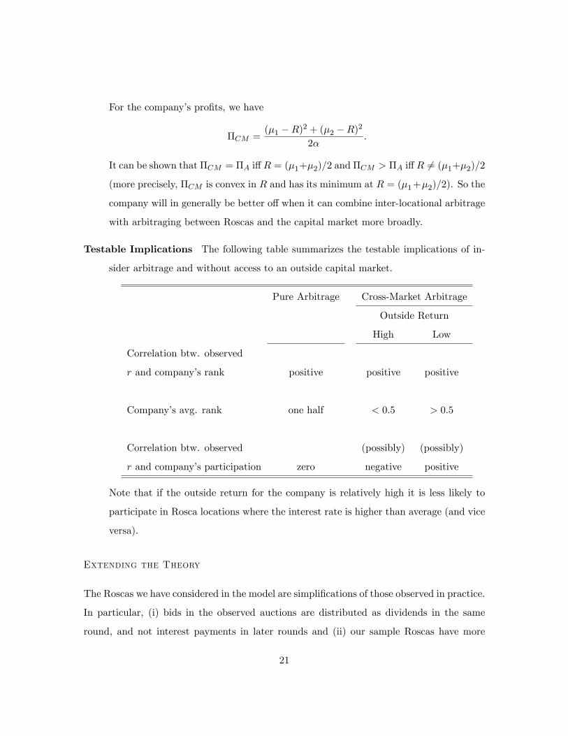
For the company�s pro�ts, we have

�CM =(�1 �R)2 + (�2 �R)2

2�:

It can be shown that �CM = �A i¤R = (�1+�2)=2 and �CM > �A i¤R 6= (�1+�2)=2

(more precisely, �CM is convex in R and has its minimum at R = (�1+�2)=2). So the

company will in generally be better o¤ when it can combine inter-locational arbitrage

with arbitraging between Roscas and the capital market more broadly.

Testable Implications The following table summarizes the testable implications of in-

sider arbitrage and without access to an outside capital market.

Pure Arbitrage Cross-Market Arbitrage

Outside Return

High Low

Correlation btw. observed

r and company�s rank positive positive positive

Company�s avg. rank one half < 0:5 > 0:5

Correlation btw. observed (possibly) (possibly)

r and company�s participation zero negative positive

Note that if the outside return for the company is relatively high it is less likely to

participate in Rosca locations where the interest rate is higher than average (and vice

versa).

Extending the Theory

The Roscas we have considered in the model are simpli�cations of those observed in practice.

In particular, (i) bids in the observed auctions are distributed as dividends in the same

round, and not interest payments in later rounds and (ii) our sample Roscas have more

21

than two rounds. Nonetheless, the testable implications derived for our simpli�ed model

generalize to auctions that take the observed Rosca rules more literally (under certain

assumptions).

More speci�cally, our model considers locations with di¤erences in aggregate productiv-

ity that are known before the Roscas commence �and are observed by the company. One

might be concerned about situations where the di¤erences in productivity across locations

are not know ex-ante. In a world with multi-period Roscas, for instance, such uncertainty

may be even more of a concern. We imagine pure arbitrage occurs by taking positions in

several Roscas and then borrowing from those with interest rates lower than the expected

average for the entire economy and saving in those with interest rates higher than that

average. Further, the information requirements for cross arbitrage are reduced relative to

the pure arbitrage case considered above. With cross arbitrage, the arbitrageur simply

needs to bid according to her outside return; i.e. borrow when the implied borrowing rate

in the Rosca is lower than the outside return, and save otherwise. Note, however that we

have assumed that the arbitrageur is risk-neutral �and indeed the theoretical results would

generalize with many risk-neutral arbitragers � but arbitrage in face of location-speci�c

uncertainty would be limited if the arbitrageurs were all risk averse.

4 Results

Financial Fragmentation

We �rst explore the extent of fragmentation of interest rates accross space. Towards this

we estimate

rdij = ai + udij

by OLS, where d indexes denominations, i branches, and j Rosca groups of denomination d

in branch i. The interest rate r is computed for each Rosca in our sample according to (1).

The resulting branch means bai are plotted in �gure 1, where a numerical branch identi�er22

is on the horizontal axis, and the (monthly) implied interest rate on the the vertical axis.

Figure 2 maps branch interest rates. Statistics of the distribution of the bai�s are set out inTable 3, column 1. Accordingly, the coe¢ cient of variation is 0.099/0.76 = 0.13. From Fig-

ure 2, the 95% con�dence interval for this sample of branch averages is roughly [0:60; 1:00],

hence its width equals almost precisely four times the standard deviation. According to

Table 3, column 1, the hypothesis of equality of all ai�s is rejected at the 1% level.

Now we will control for the denomination of a Rosca and the date when a Rosca takes

place. This is important because a Rosca of a di¤erent denomination is a di¤erent �nancial

product and the portfolio of Rosca denominations varies over branches. Moreover, even

when there is no di¤erence in interest rates over locations at any given point in time, this

interest rate may vary over time. Therefore we also control for the date at which a Rosca

was started. Our sample Roscas were started between January 2001 and October 2003. We

denote by quarterkdij a dummy variable which is equal to one for a Rosca that were started

in quarter k 2 f1; :::; 12g; where k = 1 covers the three months spell Januar to March 2001,

and zero otherwise. We estimate

rdij = �i + d +

12Xk=2

�kquarterkdij + udij : (15)

Rather than reporting the point estimates of this regression, column 2 of table 3 reports

the properties of the estimated branch intercepts. Accordingly, the standard deviation is

reduced by only about 4 percent, from 0.099 to 0.095. The hypothesis of equal interest rates

accross branches is still clearly rejected. From this exercise, we conclude that the bulk of

spatial variation fails to be explained by di¤erences in Rosca denominations or Rosca dates.

It is also interesting to note that the correlation beteween the estimated branch interecepts

in columns 1 and 2 is 0.96.

Fragmentation: Borrower Risk, Collateral Requirements and Screening

The interest rate which we used as the dependent variable in the previous estimations is

a pure savings rate. However, de facto it is an increasing function in the winning bids of

23

each rounds from 2 to n� 1 in the Rosca. Hence it is also a kind of average of the price of

funds implicit in all loans made over the course of a Rosca. An important question hence is

whether spatial di¤erences in our interest rates are due to fundamentally di¤erent borrowing

conditions in local credit markets. Such di¤erences may arise from at least two sources.

On the demand side, borrowers may exhibit di¤erent risk characteristics with respect to

repayment. On the supply side, loan o¢ cers�decisions may di¤er across locations. Both

of these sources of spatial heterogeneity remain unobserved by the researcher, however.

Luckily, data on defaults collateral and screening by the lender are in our data set. We

can hence capture relevant non-monetary characteristics of loans by the default rate, the

number of cosigners required on a loan and the screening e¤ort of the lender. The latter

is captured by an indicator which equals one if the Rosca company veri�ed occupation and

income of a borrower, and zero otherwise. Descriptive statistics of these three variables at

the Rosca level are set out in table 2. Accordingly, 4.78% of dues have not been repaid

by the time a Rosca ends, the company requires an average of 1.1 cosigners per loan and

veri�es the borrower�s income 44% of the time.

Since we are interested in explaining cross-patial variation in interest rates (and not

intra-location variation in interest rates), we will not simply add realizations of the variables

at the Rosca level to estimation equation (15). Instead we shall separately calculate branch-

speci�c �xed e¤ects for default rates and for loan terms (collateral, screening), and use these

branch-speci�c �xed e¤ects to explain the spatial variation in interest rates. Note that if

we had simply added the Rosca default rates to estimation equation (15), we would then

confound the within-branch variation with the across-branch variation. From the theory

section, however, the within-branch variation in Rosca interest rates might simply be a

function of the small number of participants in each Rosca in a speci�c location and not

due to inherent di¤erences in returns to capital across locations.

Instead, we �rst estimate equation (15) with each of the three risk measures as left hand

side variable in turn. This yields branch means net of time and denomination e¤ects. In

a second step, we use these estimated branch �xed e¤ects as explanatory variables in a

24

regression with the estimated interest-rate branch intercepts from equation (15) as the left

hand side variable. This latter regression thus has 78 observations, one for each branch.

To start out, in table 4 we have set out some descriptive statistics of the estimated

branch �xed e¤ects of three regressions (15) with default rate, number of cosigners, and

income veri�cation as the left hand side variable, respectively. According to the resulting

coe¢ cients of variation, these risk measures exhibit substantially greater spatial variation

than the interest rate (where the CV is 0.13).

Column 1 of table 5 summarizes the results of a linear regression speci�cation of the

interest rate branch �xed e¤ects on the estimated �xed e¤ects of the three loan character-

istics variables. Column 2 adds squared terms of the explanatory variables. According to

the results, only defaults are signi�cantly correlated with interest rates, where - as expected

in e.g. a Stiglitz-Weiss world - riskier borrowers have a higher willingness to pay for loans.

Column 3 of table 3 summarizes the distribution of the residuals from this regression. Ac-

cordingly, the standard deviation is reduced to 0.080 after controlling for the risk factors.

The null hypothesis of complete market integration - conditional on loan characteristics -

continues to be rejected, however.

The lower panel of that table gives p-values of tests for equal variances between pairs of

the three samples of estimated �xed e¤ects (or residuals in the case of column 3). While the

di¤erence between the �rst and the second, and the second and third speci�cations are zero,

there is, at least at the 10 percent level, a signi�cant reduction in fragmentation between

the �rst and third speci�cation. Thus risk together with controls for denomination and time

signi�cantly explain about 20 percent of spatial di¤erences in interest rates as measured by

the standard deviation. The remaining 80% remain unexplained, however.

Arbitrage

We next test if there is systematic arbitrage between locations by the company: We measure

the rank (or position) of the winner of a pot on a 0 to 1 scale, where 0 represents a receipt

of the �rst pot �and 1 represents the receipt of the last pot. More precisely, we de�ne the

25

rank of the winner of the t�th pot in the j�th Rosca of denomination d in location i as

rankdijt =t� 1Td � 1

;

where Td denotes the duration (in months) of denomination d. Descriptive statistics on the

company�s participation at the Rosca level are set out in table 2. Accordingly, the company

holds about a third of all Rosca memberships and on average occupies a rank of 0.41, which

indicates that the company on average wins pots earlier than in the middle of a Rosca. These

same variables at the branch level are set out in table 4. According to the coe¢ cient of

variation, the company�s activities exhibits spatial variation on a similar order of magnitude

as the interest rate. The mean rank of the company of .41 indicates that the company is

more interested in early than in late pots, and thus, within our theoretical framework, might

be arbitraging not only across branches but also against an outside investment opportunity

with a higher rate of return than the average in the Roscas. In all but three of the 77

branches, the institutional investor�s rank is below 0:5:

Pro�t maximizing arbitrage by the company (which reduces spatial variation in interest

rates without eliminating them) implies a positive correlation between the local interest rate

and the company�s rank in the respective location. Using only pots won by the company,

we �rst estimate

rankdijt = bi + d +12Xk=2

quarterkdij + vdijt;

where t indexes the round in a Rosca, t = 2; :::; Td. Figure 3 plots the resulting branch

�xed e¤ects bbi on the vertical axis against the estimated �xed e¤ects of (15) in its originalversion (with the interest rate as the dependent variable) on the horizontal axis. Clearly,

there is a positive relationship between these two variables. Hence,the institutional investor

takes relatively early pots (i.e. borrows) where interest rates are relatively low, and waits

to take later pots when interest rates are relatively high. We can also formally reject the

null hypothesis of no arbitrage by the company: the correlation coe¢ cient between the two

variables is 0.48 and signi�cantly bigger than zero at the one percent level. Column 3 of

table 5, moreover, shows that this positive correlation also holds conditional on other loan

26

characteristics. The estimated coe¢ cient of 1.232 suggests that an increase in the company�s

rank by one standard deviation (0.043) comes together with an interest rate that is 0.051

percentage points higher, more than half a (cross-branch) standard deviation of the interest

rate.

Barriers to Entry

So far we have argued that the results support the idea of a monopolist arbitrager (the

company) who intentionally preserves interest rate di¤erences between locations. The nat-

ural question that arises is how the company can keep out potential entrants into arbitrage.

Arbitrage is costly for potential entrants who have to pay the commission fee and provide

cosigners at the time of borrowing; while such costs are not borne by the company. In

this section, we brie�y discuss how the observed interest rate heterogeneity across space

is consistent with commission as a barrier to entry. According to the theory, competitive

costly arbitrage will drive down the interest wedge between any two locations to twice the

commission fee. As our sample Roscas have longer durations than those in the model, this

fee has to be scaled to a fee per month to make it comparable to the monthly interest

rates. Accordingly, the fee of 5% paid to the organizer by the winner of a Rosca auction

amounts to roughly 0.33% in interest rate terms per month. This is calculated as follows:

to arbitrage across any two Roscas requires an entrant to pay the commission twice, and

since the commission is paid for an average Rosca duration of 30 months, the per month

commission is 230 5%. An interest di¤erence of 0.33% between any two branches in ac-

cordance with competitive, albeit costly, arbitrage in this institutional setup. According to

table 3, column 1, the range of interest rates, 0:505; as well as the 95% con�dence band

with a width of about 0.40 is larger than 0:33. However, when we consider all possible

pairs of branches, 97% percent of pairs have a di¤erence not exceeding 0.33. The spatial

distribution of interest rates appears to be largely consistent with insider arbitrage with

costly entry, where the cost is about as large as the commission fee.

27

Within-Branch Variation

We next compare interest rate variation across branches (which has been the focus of the

paper so far) with interest rate variation within a branch. Our theoretical model predicts

that there should be no interest-rate variation within a branch (in two-period Roscas)

because the insider arbitrager equates interest rates in all Roscas each location through its

bidding. But the observed Roscas range in length from 25 to 40 rounds and the company

only takes one-third of all positions on average, leaving considerable room for auctions in

which the company has no role. So we would expect considerable unexploited variation

within Roscas as well. To measure this, we estimate

rdij = di +12Xk=2

�dkquarterkdij + udij (16)

by OLS. The residuals of this regression capture exclusively deviations of Roscas of the

same denomination in the same branch started in the same quarter. The distribution of

the error terms will arguably be due to small sample variation in the composition of Rosca

groups in the same branch and idiosyncratic shocks occuring to Rosca participants which

the limited group size is not able to smooth fully. Hence the dispersion of the residuals from

this regression capture the local interest rate dispersion (and hence fragmentation within a

location) due to the fairly small scale of of intermediation in a Rosca - a feature uncommon

to bank lending, for example. Using the same sample of Roscas underlying the results

in table 3, estimation of (16) yields a regression standard error (which equals the standard

deviation of the residuals) of 0.146. The corresponding cross-branch standard deviation of

the interest rate of 0.095 (table 3, column 2) is roughly two thirds of this �gure.

5 Conclusion

The principle of no-arbitrage, so crucial to economic reasoning, implies that risk-adjusted

interest rates should be equalized across �nancial markets. We have presented evidence

to the contrary. The �nancial markets we study are those organized in di¤erent towns

28

in the South Indian state of Tamil Nadu. The interest rates we analyze are determined

by local auctions. These interest rates accrue to savers who face an identical risk across

markets. What is remarkable about this variation in interest rates is that it persists despite

the presence of an inside arbitrager who borrows in low-interest locations and saves in

high-interest locations. We provide an explanation for why this arbitrager may deliberately

choose to maintain the interest rate spread at the cost of �nancial e¢ ciency and discuss

entry barriers into arbitrage that enable such monopoly pro�ts.

Our results raise questions about the competition between the organized (and regulated)

Roscas in our study and the commercial banking sector. One might expect then that the

variation in interest rates between �nancial markets may depend partly on the presence of

bank branches in those locations. In ongoing research we are studying whether the presence

of bank branches reduces the �nancial ine¢ ciencies across markets. Relatedly, it would be

useful to understand if the liberalization of the Indian economy in the 1990s has promoted

more e¢ cient �ow of �nance across markets. By historically studying the evolution of

interest rates across Rosca locations we hope to provide an insight into this question.

References

[1] Anderson, S. and J. Baland, 2002: The Economics of Roscas and Intrahousehold

Resource Allocation, Quarterly Journal of Economics, 117(3); 963� 995.

[2] Banerjee, A. and K. Munshi. 2004: How E¢ ciently is Capital Allocated? Evidence

from the Knitted Garment Industry in Tirupur.�Review of Economic Studies 71(1):19-

42.

[3] Banerjee, Abhijit and Esther Du�o (2005), �Growth Theory Through the Lens of

Development Economics,� chapter 7 in the Handbook of Economic Growth Vol. 1A,

P.Aghion and S. Durlauf, eds., North Holland.

[4] Besley, T., S. Coate and G. Loury. 1994: Rotating Savings and Credit Associations,

Credit Markets and E¢ ciency. The Review of Economic Studies, 61(4): 701-719

29

[5] Borenstein, Severin, Knittel, Christopher R. and Wolfram, Catherine D., 2008. Ine¢ -

ciencies and Market Power in Financial Arbitrage: A Study of California�s Electricity

Markets. The Journal of Industrial Economics, Vol. 56, Issue 2, pp. 347-378.

[6] de Mel, S., Mckenzie, D. and C. Woodru¤, Returns to Capital in Microenterprises:

Evidence from a Field Experiment. forthcoming, Quarterly Journal of Economics.

[7] Klenow, P. and C-T Hsieh, forthcoming "Misallocation and Manufacturing TFP in

China and India" Quarterly Journal of Economics

[8] Eeckhout, J. and K. Munshi, 2004: Economic Institutions as Matching Markets. Man-

uscript, Brown University.

[9] Paulson, Anna L., Robert Townsend and Alex Karaivanov 2006: Distinguishing Limited

Liability from Moral Hazard in a Model of Entrepreneurship," Journal of Political

Economy Vol. 114. No. 1, pp. 100 -144

[10] Shleifer, A. and R. Vishny 1997. The Limits to Arbitrage. Journal of Finance, 52:1,

35-55.

30

Table!1.!Descriptive!Statistics,!Rosca!DenominationsDuration!(Months)

Contribution!(Rs./month)

Pot!(Rs.) FrequencyRelative!

Frequency25 400 10,000 488 23.7425 600 15,000 8 0.3925 800 20,000 9 0.4425 1,000 25,000 278 13.5225 2,000 50,000 214 10.4125 4,000 100,000 80 3.8925 8,000 200,000 2 0.1025 12,000 300,000 1 0.0525 20,000 500,000 3 0.1530 500 15,000 282 13.7230 1,000 30,000 98 4.7730 1,500 45,000 2 0.1030 2,000 60,000 22 1.0730 2,500 75,000 11 0.5430 3,000 90,000 7 0.3430 4,000 120,000 1 0.0530 5,000 150,000 53 2.5830 10,000 300,000 22 1.0730 20,000 600,000 4 0.1930 25,000 750,000 1 0.0530 30,000 900,000 2 0.1040 250 10,000 176 8.5640 375 15,000 1 0.0540 500 20,000 3 0.1540 625 25,000 85 4.1340 750 30,000 2 0.1040 1,250 50,000 77 3.7540 1,500 60,000 3 0.1540 2,500 100,000 99 4.8240 3,750 150,000 2 0.1040 5,000 200,000 4 0.1940 7,500 300,000 4 0.1940 12,500 500,000 4 0.1940 12,500 500,000 3 0.1540 15,000 600,000 1 0.0540 25,000 1,000,000 4 0.19

Sum 2056 100.00

Table!2.!Descriptive!Statistics,!Sample!Roscas

Mean Std.!Dev. Minimum MaximumDuration!(months) 29.64 5.99 25.00 40.00Contribution!(Rs./month) 1,468.12 2,462.76 250.00 30,000.00Pot!(Rs.) 44,277.72 81,223.17 10,000.00 1,000,000.00Date!of!first!auction August!30,!2002 181!(days) Jan!2,!2002 Sept!13,!2003Monthly!Interest!Rate!(%) 0.74 0.22 0.00 1.59Default!Rate!(%) 4.78 2.55 0.00 19.68Cosigners 1.10 0.62 0.00 3.89Income!Verification 0.44 0.25 0.00 0.97Company!Participation 0.32 0.19 0.00 0.95Company!Rank 0.41 0.10 0.08 0.83

Number!of!observations:!2,056

Table!3.!Monthly!savings!rates,!summary!of!estimated!fixed!effects/residuals

Without!Controls With!Controls Net!of!Defaults,(time,!denomination) collateral,!screening

(1) (2) (3)Mean 0.760Standard!Dev. 0.099 0.095 0.080Range 0.505 0.475 0.463Test!for!Equality!(p) 0.000 0.000 0.000

Test!for!Equal!Variances!(p"value):!!!!!!!(1)!and!(2) 0.716!!!!!!!(1)!and!(3) 0.069!!!!!!!(2)!and!(3) 0.147

Number!of!observations:!78

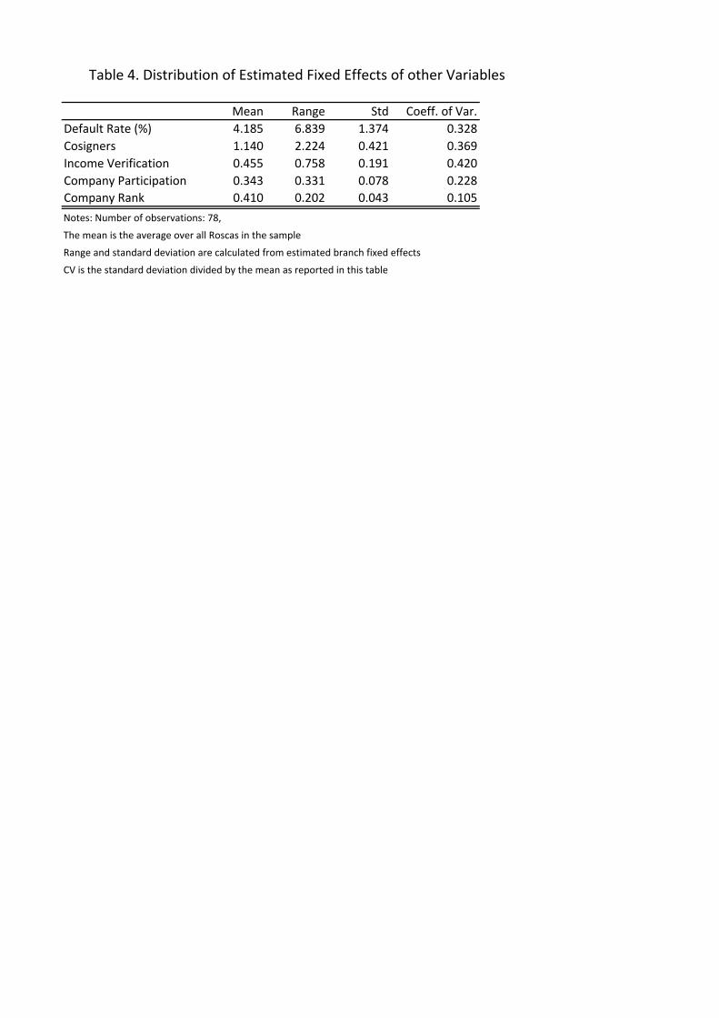
Table!4.!Distribution!of!Estimated!Fixed!Effects!of!other!Variables

Mean Range Std Coeff.!of!Var.Default!Rate!(%) 4.185 6.839 1.374 0.328Cosigners 1.140 2.224 0.421 0.369Income!Verification 0.455 0.758 0.191 0.420Company!Participation 0.343 0.331 0.078 0.228Company!Rank 0.410 0.202 0.043 0.105

Notes:!Number!of!observations:!78,

The!mean!is!the!average!over!all!Roscas!in!the!sample

Range!and!standard!deviation!are!calculated!from!estimated!branch!fixed!effects

CV!is!the!standard!deviation!divided!by!the!mean!as!reported!in!this!table

Table!5.!Explaining!Spatial!Interest!Rate!DifferencesDependent!Variable:!Branch!intercepts!from!interest!rate!regression

(1) (2) (3)Intercept 0.666 *** 0.805 *** 0.418 ***

(0.045) (0.093) (0.091)Defaults 0.028 *** "0.042 0.001

(0.007) (0.030) (0.008)Defauts!Squared 0.009 **

(0.004)Cosigners 0.034 "0.003 0.038

(0.023) (0.131) (0.021)Cosigners!Squared 0.016

(0.045)Screening "0.083 "0.122 "0.110

(0.052) (0.359) (0.053) **Screening!Squared 0.036

(0.313)Company's!Participation "0.599 ***

(0.142)Company's!Rank 1.232 ***

(0.284)

R"Squared 0.23 0.24 0.42Number!of!observations 78 78 78

Notes:all!explanatory!variables!are!estimated!branch!fixed!effects!from!a!regression!of!the!explanatory!variable!on!branch!FEs!denomination!and!time!dummies

Figure!1.!Distribution!of!Branch!Interest!Rates

Figure!2.!Map!of!Branch!Interest!Rates

Figure!3.!Scatter!Plot!of!Company's!Rank!and!Local!Interest!Rates

Figure!4.!Scatter!Plot!of!Company's!Participation!and!Local!Interest!Rates