133

William A. Barnef I and Ge Zhou

William A. Barnett is a professor of economics at WashingtonUniversity, St Louis. Ge Zhou recently received a doctorate ineconomics from Washington University, St Louis. Research onthis project was partially supported by NSF grant SES 9223557We wish to thank William Brainard for his comments, whichsubstantially influenced the final revision of this paper

Financial Firms’ Productionand Supply-Side MonetaryAggregation Under Dynamic

Uncertainty

HIS PAPER IS FOCUSED ON the productiontheory of the financial firm and supply-sidemonetary aggregation in the framework of dy-namics and risk. On the demand side, there hasbeen much progress in applying consumer de-mand theory to the generation of exact mone-tary aggregates and integrating them intoconsumer demand system modeling~However,on the supply-side, monetary services areproduced by financial firms through financialintermediation, and, hence, exact supply-sidemonetary aggregation must be based uponfinancial firm output aggregation. Most of theliterature on exact aggregation theory is basedupon perfect certainty, which often is a reasona-ble assumption regarding contemporaneous con-sumer goods allocation decisions. Risk, however,is an important consideration in modeling thedecisions of financial intermediaries. Further-more, that risk not only applies to future prices

and interest rates, but also to contemporaneousinterest rates and thereby to the contemporane-ous user costs of produced monetary services.In this paper we derive a model of financialfirm behavior under dynamic risk, and we findthe exact monetary services output aggregate.We estimate the Euler equations that comprisethe first-order conditions for optimal behaviorby financial firms.

Barnett (1978,1980) introduced economicaggregation and index number theory to demand-side monetary aggregation by applying Diewert’s(1976) results on superlative index numbers. Theproposed Divisia index in Barnett’s work is anelement of Diewert’s superlative index numberclass. Analogous to demand-side monetary aggre-gation, Hancock (1985,1987), Barnett (1987), andBarnett, Hinich and Weber (1986) have providedresults on supply-side monetary aggregation.2

They use neoclassical economic theory to model

1See Barnett, Fisher and Serletis (1992).2Demand-side” and supply-side” imply respectively thedemand tor monetary services by consumers and manu-facturing firms, and the production of monetary services byfinancial intermediaries. Barnett (1987) has shown that con-sumer’s demand for money and manufacturing firm’s de-mand for money result in the identical aggregationproblem, at least in the perfect certainty case. However,supply-side aggregation of produced monetary services

creates uniquely different aggregation problems resultingfrom the existence of required reserves, which alter theuser cost of produced monetary services. For furtherresults regarding demand for monetary services bymanufacturing firms, see Robles (1993) and Barnett andVue (1991).

MARCH/APRtL 1994

134

financial firms’ production, so the existing eco-nomic aggregation and index number theory aredirectly applicable. In fact, throughout the litera-ture on applying economic aggregation and in-dex number theory to monetary aggregation,researchers usually assume perfect certainty.Exceptions are Barnett and Yue (1991) and Poter-ba and Rotemberg (1987), who generalize todemand-side exact monetary aggregation underrisk. Supply-side monetary aggregation underrisk has not previously been the subject ofresearch.

Introduction of dynamics and uncertainty intosupply-side monetary aggregation requiresextensions of earher research in this area. Afinancial firm’s portfolio is generally diversifiedacross different investment instruments, and theportfolio’s rate of return is unknown at the timethat the investment decision is made. Hence, theassumption of perfect-certainty and single-periodmodeling is not appropriate. Furthermore, super-lative index numbers, such as the discrete timeDivisia index, have known tracking ability onlyunder the assumption of perfect certainty. In thispaper, we develop a dynamic approach to supply-side monetary aggregation under uncertainty.

Historically, the literature on financial inter-mediation has produced many diverse models,often linked only weakly with neoclassical eco-nomic theory and having various objectives. Theearly view of the creation of money by financialfirms, primarily viewed to be banks, was thedeposit multiplier approach. By this theory in itsoriginal form, the process of creating money issimply determined by the reserve requirementratio. Another approach is based upon theMiller-Modigliani theorem, which asserts theirrelevance of financial firms to the real econo-my in a setting of a perfect capital market. Inrecent years, many economists have questionedthe appropriateness of either of those two verydifferent propositions and attempts have beenmade to extend those theories by weakening theunderlying assumptions.

Another approach is based upon the capital-asset pricing model (CAPM). Under the assump-tions of that model, either the financial firm’sportfolio rate of return is normally distributedor investors have a quadratic utility function de-fined over end-of-period wealth. Under either of

those assumptions, the financial firm’s optimalportfolio behavior can be represented by max-imizing utility over the portfolio’s expected rateof return and variance. This approach has beenuseful in modeling the optimal portfolio allocationdecision conditionally upon the real resource in-puts, which are not explained endogenously.Another important approach is represented byDiamond and Dybvig (1983). They apply tradi-tional consumption-production theory and usean intertemporal model subject to privately ob-served preference shocks to examine the equi-librium between banks and depositors. Thestudies in this tradition have been successful inexplaining bank runs. However, banks, servingsolely as a production technology to depositors,play only a passive role in that approach.

Another approach is represented by Hancock(1985, 1987), Barnett (1987), and Barnett, Hinichand Weber (1986). They treat the financial inter-mediary in the same manner as a conventionalproduction unit and use neoclassical firm theoryto model a financial intermediary’s productionof output services and employment of inputssubject to the firm’s technological feasibility con-straint.3 This approach fully models the roleplayed by financial firms as producers of mone-tary services. Moreover, it provides the neededtools to apply existing economic aggregation the-ory to aggregation over financial firms’ outputmonetary services, which comprise the econo-my’s inside money. However, those studies havenot developed a dynamic model of financialfirms’ production under uncertainty. This paperprovides that difficult extension of financial firmmodeling and output aggregation under neoclas-sical assumptions with dynamic risk.

With the theoretical model of a financialfirm’s monetary services production and thederived exact theoretical output aggregate, weestimate the model’s parameters and test forweak separability of output services from factorinputs. We then substitute the parameter esti-mates into the weakly separable output aggrega-tor function to generate the estimated exactsupply-side monetary aggregate.4 lb this end,we develop a procedure for testing weakseparability and for estimating the parametersof a flexible functional form specification ofbank technology. The estimation is accomplished

3The papers of Tobin (1961) and Brainard and Tobin (1963,1968) were the first to argue forcefully for the use of micro-economics and equilibrium theory in modeling the financialfirm.

4Diewert and Wales (1987) and Blackorby, Schworm andFisher (1986) have illustrated the difficulty of maintainingflexibility, regularity and weak separability simultaneously.

FEDERAL RESEF yE BANK OF ST. LOWS

135

through Hansen and Singleton’s (1982) general-ized method of moments approach to estimatingEuler equations.

Our empirical results are based upon com-mercial banking data. Our evidence indicatesthat banks’ outputs are weakly separable fromfactor inputs in the transformation function.Moreover, even under uncertainty, the Divisia in-dex provides a better approximation to theestimated theoretical aggregate than does thesimple-sum or CE index.~These findings supportthe existence of a supply-side monetary ag-gregate and the potential usefulness of theDivisia index to aggregate over the weaklyseparable monetary assets on the supply side ofmoney markets. The result is a measure of in-side money, in the sense of monetary servicesproduced by private financial firms.

The paper proceeds as follows. In the nextsection, we construct our theoretical model ofmonetary service production by financial firmsunder dynamic uncertainty The model reducesto a dynamic stochastic choice problem, forwhich we derive the Euler equations. In thethird section, we present our approach to flexi-ble parametric specification, weak separabilitytesting and parameter estimation using Hansenand Singleton’s (1982) generalized method of mo-ments estimation. The fourth section formulatesthe empirical application using banking industrydata. The fifth section contains the empiricalresults, including parameter estimates, weakseparability test results, the estimated theoreticalaggregate, and the comparison among indexnumber approximations to the estimated exactaggregate, where the index numbers consideredinclude the Divisia, simple-sum and CE indexes.Section 6 brings together the demand side withthe supply side to investigate the implications ofour model in general equilibrium. Section 7 pro-vides a graphical illustration of the errors-in-the-variables problem produced by the use of thesimple-sum index as a measure of the monetaryservice flow. The final section presents a fewconcluding remarks.

THEORETICAL MODELIn this section, we derive our theoretical model

of monetary services production by financialfirms under dynamic uncertainty Consider afinancial firm which issues its own liabilities andreinvests the borrowed funds in primary finan-cial markets. In this process, real resources suchas labor, materials and capital are used as fac-tors of production in creating the services ofthe produced liabilities. Those produced liabili-ties are deposit accounts providing monetaryservice combinations that would not have exist-ed in the economy without the financial firm.The liabilities of the financial firms include, forexample, demand deposits and passbook ac-counts, and are assets to the depositors. Thevalue added through the creation of those assetsby a financial intermediary is that firm’s contri-bution to the economy’s inside money services.Without the existence of financial firms and theaccounts that they create, investors in moneymarkets would be limited to the use of primarymoney-market securities as the short maturityassets in their portfolios. While the producedliabilities of financial firms may not appear tobe “outputs” to an accountant looking at thefirm’s balance sheet, the produced liabilities offinancial firms are the outputs of the firms’production technologies.°

The financial firm’s profits are made from theinterest rate spread between the financial firm’sfinancial assets (loans) and the firm’s producedliabilities. That spread must exceed the realresource costs, in order for the firm to profitfrom its operation. Let Y, be the real balances ofthe financial firm’s asset (loan) portfolio duringperiod t.

7 Let R, be the portfolio rate of return,which is unknown at the beginning of eachperiod. Financial firms also hold excess reservesin the form of cash, which has a nominalreturn of zero. The real balance of cash holdingis C,. Let y~,be real balances in the firm’s ithproduced account type and h~be holding costper dollar for that liability, where i’~’1,-~,L

8Theamount of the jth real resource used is z~,and

5The formula for computing the Divisia index is in Barnett(1980). Further details regarding the data sources usedwith the index are in Thornton and Yue (1992), who alsoprovide instructions on downloading the data from the Fed-eral Reserve Bank of St. Louis’ public electronic bulletinboard, called FRED. The formula for computing the CE(‘currency equivalent”) index is in Rotemberg, Driscoll andPoterba (1991).

°SeeBarnett (1987).7As used in this paper, portfolio is the sum of allinvestments.

8The holding cost lift is defined as h1,=r~,÷R,kt.In this for-mula, r~is the account’s net interest rate, which is definedsuch that all the benefits (for example, service charges)and costs (for example, deposit insurance) generated bythe borrowed funds have been factored into the interestrate, and R,k1, is the implicit tax rate on the financial firmfrom the existence of a reserve requirement on that ac-count type. Required reserves are assumed to yield nointerest and hence, produce an opportunity cost to thefinancial firm, since the firm otherwise could have investedthe required reserves at a positive rate of return.

MAROII/APRtL 1994

136

its price is wp, where j=1)..,J. Let P, be thegeneral price index, which is used to deflatenominal to real units. All financial transactionsare contracted at the beginning of each period,but interest is paid or received at the end of theperiod. The cost of employing resource ~ ispaid at the start of the period.

The firm’s variable profit at the beginning ofperiod t in accordance with Hancock’s (1991,equation 3.1) formula, is

(1) ii~, = (i+ii,~) Y,1P,,—Y,P,+C,,P,

1--C~P,

+ 5 [y,,P,—(i+h,,)y,,,P,,] —~

i—i f—I

The first two terms in equation I represent thenet cash flow generated from rolling over theloan portfolio during period t. The third andfourth terms represent the change in the nomi-nal value of excess reserves. The fifth term isthe net cash flow from issuing produced finan-cial liabilities. The last term is total payments forreal resource inputs.

Portfolio Y, investment, however, is constrainedby total available funds, under the assumptionthat all earnings are paid out as dividends. Therelationship is

(2) 1~P, ~ (i—k1,) y,,P,—C,P,— ~1=l f—I

where k1, is the reserve requirement ratio forthe ith produced account type, with 0 k1, 1.

Rearranging, equation 2 can be seen to state

that total deposits ~ y,,P,, are allocated to

required reserves, excess reserves, investment inloans, and payments for all real resource inputs.Substituting 2 into I to eliminate 1’,, we obtainthe firm’s profit function subject to its balancesheet constraint:

(3) ir, = ~ [E(i+R,_,) (1—k, ,_~)

/—i

— (i+h, ,~)]y1,3~,+k,~y11I~}

— ~ (1 +R,,) 145, ,1z1 ,~, -

f—I

We assume the financial firm chooses the levelof borrowed funds, excess reserves, and realresource inputs to maximize its expected dis-counted intertemporal utility of variable profits,

subject to the firm’s technology. We further as-sume the financial firm’s intertemporal utilityfunction is additively separable. l’hen, the firm’smaximization problem can be expressed by thefollowing dynamic choice problem:

(4) Max E,[>1 (_iu_) s—i U(ir)]s-I

si. C)(y,, , .., y,~,C~,z Is~ , z,,) = 0V S t,

where E, denotes expectation conditional on theinformation known at time t, p is the subjectiverate of time preference and is assumed to beconstant, U is the utility function, ir, is the vari-able profit at period s given by equation 3, andC) is the firm’s transformation function, definingthe firm’s efficient production technology from

(5) 0(y1, ,..-, .v,~C5, z,,,, z,,) =0 V s t.

In accordance with the usual properties of aneoclassical transformation function, C) is con-vex in its arguments. In addition, the inputs aredistinguished from the outputs by the inequalityconstraints:°

0, o Vj=1aç 3%

and

0 V i=1 ,.., L

We also assume that C) is continuous andsecond-order differentiable.

Substituting equation 3 into 4, we have

(8) Max E, ~ (——)‘‘U(~ {UI+R,,) (1-k,,,)

—(i+h1 ,_~y,-,,1

P,1

+k1

y11

P,}

—R51

C,,P,,—~ (1+R,,) ,1z~, f_1)}

st. C)(y11,..., y,,, C~,z,1,..., z,,) = 0 V s t.

We now proceed to derive the Euler equations,comprising the first-order conditions, for thisstochastic optimal control problem. We useBellman’s method. To do so, we must put the de-cision into Bellman’s form, which requires iden-tifying the state and control variables anddetermining that the decision, stated in terms ofthose variables, is in the form providing knownEuler equation structure.

9See Barnett (1987), Hall (1973) and Diewert (1973).

FEDERAL RESERVE SAN-K OF ST. LOINS

137

We assume that the financial firm behavescompetitively so that the prices h,3, andare taken as given by the firm. In addition, h,3,and w~31are nonstochastic, since they are laggedone period. From the same perfect competitionassumption, it follows that R,, k

15, and i~are

random processes that are not controllable bythe firm. We select as state variables duringperiod 5: y,5, V i, z, V j, C1, H,, H, k13, h13,V i ~ Vj, P

11, and P

1. We choose y1, V i and

z~Vj to be the control variables during period s.

Define w to be the vector of all of the statevariables, and define u to be the vector of allcontrol variables. Let A be the subset of statevariables defined by A3 = (Rd k~,h,

3, V i, ~

V j,P1). We assume that A, follows a first-order

Markov process, with transitions governed bythe conditional distribution function F1A1 IA3).Hence, the transition equation for state variables(R

3,, R3, k~,hjg_1 V i, ~ V j, P,_,, P) is im-

plicitly defined by F(A141JA5). The transitionequations for y,,, V i and z1,, V j are the trivialidentities

(9) y,~= y~,V

and

(10) z~.= V s.

The role played by these two equations in ourapplication of Bellman’s method follows from thefact that each of the variables in equations 9and 10 are included both among the controland state variables, although with a time shiftdistinguishing them in each of their roles?0Hence, with the appropriate time shift in thesubscript, equations 9 and 10 can be viewedas connecting together some of the control andstate variables. This connection accounts for thefunction of those equations as transition equa-tions. In particular, the left-hand sides can beidentified as next-period state variables, whilethe right-hand sides can be identified as current-period control variables. Hence, each of thoseequations can be interpreted as defining theevolution of a state variable conditionally on acontrol variable. The transition equation for C3_1

is implicitly determined by the transformationfunction 5.

The objective function in equation 8 is an in-finite summation of discounted utilities of varia-ble profits, starting at period t. Recalling thetime shifts appearing in our definition of thestate and control variables during period s, wesee that the discounted utility of variable profitat period s depends only on that period’s statevariables and control variables. By examining thetransition equations, it is evident that each statevariable is a function of only previous controlsand not of previous values of the states. In par-ticular, if we let g represent the vector of alltransition functions, we can rewrite the dynamicdecision problem as

Max E, {~ (—1—)~’t][ir(w,, ii)]]

~ 1+p

st. w34, = g(u3), s t.

This dynamic problem meets all of the condi-tions to be a recursive problem in the Bellmanform. Using Bellman’s principle, we can derivethe first-order conditions for solving the dynam-ic problem 8. ‘The Bellman recursive equationis

v(w,) = max E,{L]lir,(w,, u,)IUt

+ ~ v(iv,41) J n~, st. tv,4

, =

where v(w,) is the optimized value of the objec-tive function.

The first-order conditions for the Bellmanequation are

Dir,(11) E, [— (ir,) — (w,, u,)øir, 3u,

~ )IwI= °-

1+~2 3u, ‘ Sw, 141 I

The functional form of v is unknown. However,

since !~-=o we can use the Benveniste and3w,

‘°Theuse of such trivial identities as transition equations(laws of motion) in optimal control and dynamic program-ming is not unusual. For example, it is common in optimalgrowth models to define current capital stock to be a statevariable, while next period’s capital stock is defined to be acontrol, with those state and control variables tied togetherby a trivial identity. The nontrivial dynamics is found in theobjective function of such models. See, for example, Sar-gent (1987, p. 24).

MARCH/APRfL 1994

Scheinkman equations to eliminate Th~Jw,41)?~8w,

The general form of the Benveniste and

Scheinkman equations is

SirSi’ SU(w) - (ir) .L (w, U,)Sw, Sir, ‘8w,

+ _LE,L~!~ Dv(w,, u,) (it’,

4)J-

I+p tSw, 8w,

Since = 0, the above equation impliesSw

dir(12) —~-~- (w,) = (ir) —i- (w,, U,).

Sw, 8 ‘ Sw,

Substituting 12 into 11, we get

Sir(13) E, (ir,) -~ (it’,, U,)

Sir,

+ 18W SU(U) (÷,)1+i Sii, ‘ 8;

S-n-(iv,~,,U,

91) Fw,J = 0.

8 w

A very general specification of utility torepresent risk is the hyperbolic absolute riskaversion (HARA) class, defined by

(14) U(ir,) = ~ (—p--— irp i-p

where p, h and d are three parameters to beestimated. The foliowing useful utility functionsare fully nested special cases of the HARAclass:’~

a. risk neutrality: p=i, U(ir)=hii-,,

b. quadratic: p=2, U(ir,) = —(1/2) (—hr, + d)’,

c. negative exponential: p= —co and d=i,U(ir,) = —

d. power: d=0 and p<i, U(-,r,) = (ir?/p),

e. logarithmic: d=p=o, U(ir,) = log ir,.

‘The general HARA specification for U(ir,) satis-

138

fies the relevent theoretical regularity conditionswhen the domain of U(ir,) is constrained to

{ir,: ~ ir,+d>o} with h constrained to satisfy

h >0. When p >1, absolute risk aversion (Arrow-Pratt) is decreasing, and when p >1, absoluterisk aversion is increasing. The power utilityfunction special case is very widely used. Sincethat functional form exhibits constant relativerisk aversion (CRRA), the power utility functionoften is called the CRRA or isoelastic case?3

Differentiating (14) with ir,, we get

(15) -~-~ = h (—p--— ir,+df’,8; I-p

Using equations 13 and 15 along with the de-fined state variables, control variables and tran-sition equations, we obtain

(16) E,{i~k~(_!L 11-+w~’1-p

and

+P,—1---- [(1+R) (1—k,,)—(i+h,)1+p

SQ/Dy (JL. +d)}+ B, - rn ~~i-p

= 0 Vy,1, i=1,...,I

(17) E,[P1B,5 Q/Szk (_IL. ir,91+d)~SQ/DC, i—p

— - ir,91+d)(I+R)~,

= 0 Vz,,,j=1,...,J.

Equations 16 and 17 are a system of I+inonlinear equations. Theoretically from 16 and17 plus the transformation function 5, wecould solve for (Y11, ..., Y,,, C,, Z,,, ...,z,,).However, in practice the solution could beproduced only numerically, since a closedform algebraic solution rarely exists for suchEuler equations.

11See Sargent (1987) for an excellent presentation of dynam-ic programming.

‘2See Ingersoll (1987, pp. 37-40). In case (d) below, imposingthe restriction d—O alone on equation 14 will not producethe exact form provided for the power function. However,the form acquired subject to that sole restriction is a posi-tive affine transformation of the power function. Hence bothforms represent the same risk behavior.

13See, for example, Barnett and Yue (1991).

FEDERAL RESERVE SANK OF St LOWS

139

Sir, 1911+12 dir, ‘~‘ 8z,, (w,91,

- SQ/8z SU

Sd/ac (w,, U) ~

Sir,(it’,

91, U,

91)]] = 0

SC,,

“While the risk-neutral case is acquired directly by makingthose substitutions in the original decision problem, theresulting Euler equations are not acquired simply by mak-ing those substitutions in the risk-averse Euler equations,16 and 17. The reason is that a cancellation within theEuler equations that is produced when the rate of discountis the constant, p. does not apply when the rate of dis-count becomes the variable, R,. In particular, after replac-ing p with 1.Q and p with R,, it also is necessary tomultiply the two terms within equation 17 by 1I(li-R,) to getthe risk neutral case Euler equations. No such adjust-

ment is needed within equation 16, since no relevant fac-tors cancelled out in the derivation of equation 16. Thisobservation also is relevant to the risk-neutral Euler equa-tions 80 and 81 below.

lSSee, for example, Debreu (1959, ch. 7) and Duffie (1991,section 6.3). Regarding the complications produced by in-complete markets, see Magill and Shafer (1991, section 4).

and

SU S-zr(20) K, {— (ir,) —..—~ (w,, ti)Sir, 871

In the following discussion, we extend thedynamic decision 8 into the more general caseincorporating learning by doing technologicalchange. In the econometric literature on es-timating returns to scale in manufacturing,increasing returns to scale usually are found,despite the fact that increasing returns to scaleviolates the second-order conditions for profitmaximization. We believe that a likely source ofthis paradox is the potential to confound techno~logical change with returns to scale, whenlearning by doing technological change existsbut is not incorporated within one’s model.

Let y, be the vector of y,, for all i and z, bethe vector of z,, for ali j. We then write themaximization problem as

(18) Max E,[~ (_.L)~’U(ir)]1+p

Q(y,, C,, z,, J’3~I) = 0 V

The appearance of y31 in the transformationfunction represents learning by doing. Firmtechnology improves through experience.

At the present stage of this research, we arenot using the learning by doing extension of ourmodel in our empirical work, so we only pro-vide the Euler equations below, without supply-ing the details of the derivation. Those Eulerequations under learning by doing are

(19) E,[ 42 (ii) -i: (w,, U)

1 SU Sir,+ -j—~-—[-a-- (iç91

)5~

1-, (w,91, U,÷

1)

i 8Q/Sy,~,— i+p SQ/SC, ~t’I+if ~1+l

SU Sir,(ir,÷3) (w,92, ti,93

)Sir, SC,,

5~8Y~( )DU(— SQ/SC, ii~, U, -

r (w U,÷)]] = 0

Vz,

Equations 19 and 20 are generalizations of(16) and (17). If learning by doing is excluded byimposing SQ/Sy, l=0, then (19) and (20) reduceto (16) and (17), respectively. In the rest of thecurrent paper, we return to the special case ofno technological change.

A further nested special case is also interest-ing. We acquire risk neutrality by setting p = 1.As is conventional under risk neutrality dis-counting is acquired objectively by replacing thesubjective rate of time discount, p, by RtY4 Onereason for interest in that special case is that, ingeneral equilibrium theory, the assumption ofcomplete contingent claims markets combinedwith perfect competition can be shown, undercertain additional assumptions, to produce theconclusion that firms wili be risk neutral, evenif their owners are risk-averse. The risk aversionof the owners then is captured within thecontingent claims prices, which are taken asgiven by the firms’ managers under perfectcompetition?~

While this theoretical issue is interesting, wedo not consider it alone to be a convincing rea-son to impose risk neutrality on the manage-ment of an industry that behaves in a mannerexhibiting clear risk aversion. However, we areinterested in that fact that the Divisia index,along with virtually all of the literature on indexnumber theory is produced under the assump-tion of perfect certainty. This fact would suggestthat the tracking ability of such index numbersmay degrade as the level of risk aversion in-

MAROM/APRiL 1994

140

creases. Hence, we produce results both withand without risk neutrality imposed, as a meansof exploring the extent to which the trackingability of index numbers is degraded in the riskaverse case relative to the risk-neutral case.

Under risk neturality our Euler equations

reduce to’°

(19’) E[P B,(1—k,) — r,, + ~ ~ SQ~’3y311+R, ‘ 1+R, SQ/ac,

and

= 0 V j’,,, i=1,...,J

-. IL 30/8 -(20 )L,[P, 1+R, DQ/3c, ~ = 0 V ¶j=1 ,...,.J.

The assumption of perfect competition is itselfsufficient for the existence of a representativefirm. See Debreau 1959, p. 45, result 1. Hence,the theory acquired from our model can beapplied with data aggregated over banks?’

SIJrPLY~s:l1)EMONETARY.A.GGREG.~-YFION.ANI.) A WE.A.K

SEPA.RABLEJTY ‘FEET

Having formulated our dynamic model offinancial firm production under uncertainty andhaving derived the Euler equations, we can pro-ceed to investigate the exact supply-side mone-tary aggregates that are generated, if the firm’soutput monetary services are weakly separablefrom inputs.

SuppIv~ShIe4gflf3pp~~flfl

Most money in modern economies is insidemoney which is simultaneously an asset and aliability of the private sector. Inside money pro-vides net positive services to the economy as aresult of the value added that is created by the

financial intermediation that produces the insidemoney In our model, the borrowed funds thatare outputs produced by financial intermediariesare inside money Inside money may take vari-ous forms such as demand deposits, interest-bearing checking accounts, small time deposits,and checkable money market deposit accounts.The sum of the dollar value in such accountsdoes not measure the services of inside moneyany more than the sum of subway trains androller skates measures transportation services,since the components of the aggregate are notperfect substitutes. The aggregation-theoreticexact quantity aggregate does, however, measurethe service flow?~

The procedures involved in identifying andgenerating the exact quantity aggregates ofmicroeconomic theory are described in detailby Barnett (1980). The approach necessarilyinvolves two steps: identification of the compo-nents over which exact aggregation is admissibleand determination of the aggregator function de-fined over those components. The first step de-termines whether or not an exact aggregateexists, and the second step creates the exact ag-gregate that is consistent with microeconomictheory. The second step cannot be appliedunless the first step succeeds in identifying acomponent cluster that satisfies the existencecondition. That existence condition, which is thebasis for the first stage clustering of compo-nents, is blockwise weak separability. In accor-dance with the definition of weak separability, ablocking of components is admissible if and onlyif the goods in the block can be factored outof the structure of an economy through a sub-function. In other words, it must be possible toformulate the economic structure in the formof a composite function, with the goods in thecluster being the sole variables entering into theinner function of the structure. If that condition

leobset-ve that only one time subscript exists in the risk-neutral Euler equations, so that the solution becomes stat-ic. Once the nonlinear utility function has been removedfrom the objective function, the terms with common timesubscripts can be grouped together. However, under riskaversion, even under our assumption of intertemporalstrong separability, more than one time subscript exists wi-thin the utility function for each time period, since bothcurrent and lagged t appear as subscripts in equation 3for each value of profit, ‘r,. Hence, the dynamics found wi-thin the objective function of equation 4 cannot be re-moved by regrouping terms.

“In fact, Debreu’s theorem can be used to aggregate overall firms of all types in the economy to produce the ag-gregated technology of the country. The representative firmmaximizes profits subject to that aggregated technology.However, we use the theorem only to aggregate over the

firms in one industry. It should be observed that the easeof aggregation over firms under perfect competition is inmarked contrast with the complexity of the theorems onaggregating over consumers.

‘8See, for example, Blackorby, Schworm and Fisher (1986)regarding the importance of using appropriately aggregatedoutput data from firms.

FEDERAL RESERVE SANK OF St LOWS

141

is satisfied, an exact quantity aggregate existsover the goods in the cluster and the aggregatorfunction that produces the exact aggregate overthose goods is the inner function within thecomposite function.

Let y=(y1,,...,y,,)’ and x=(C,, z,,,...,z,,)’ where yis the vector of the firm’s outputs and x is thevector of the firm’s inputs. The transformationfunction becomes

Q(yx)=0.

An exact supply-side aggregator exists over all ofthe elements of y if and only if y is weaklyseparable from x within the structure of Q.Mathematically, that statement is equivalent tothe existence of two functions H and y0 suchthat

Q(yx) =

where y0(y) is a convex function of y.’~In aggre-gation theory y0(y) is called the output aggrega-tor function. Furthermore, suppose that y0 (y) islinearly homogeneous in y. Under this assump-tion, if each y, grows at the same common rate,the theoretical aggregate y

0(y) will grow at that

rate. Clearly, without that condition, y0 (y) couldnot serve as a reasonable aggregate.10

As shown by Leontief (1947a, 1947b), theweak separability condition is equivalent to

(21) —~— (SQ(v~x)/SY1)= 0 for all k.Sick 8Q(y,x)/Dy1

If a subset of the components of y were weaklyseparable from all of the other variables in Q,then an exact output aggregate would exist onlyover the services of that subset of componentsand not over the services of all outputs. If wecan test for the separability structure of thetransformation function and acquire the func-tional form of y0(y), when y is weakly separablefrom x, then we could estimate the parametersof y0 (y) to acquire an econometric estimate ofthe exact output aggregate.

Although aggregation theory can provide uswith the tools to estimate the exact aggregatorfunction, the resulting aggregate is specificationand estimator dependent. Alternatively theliterature on statistical index number theoryprovides nonparametric approximations to aggre-gator functions when the existence of the aggre-gator can be demonstrated through a weakseparability test. Statistical index numbers pro-vide only approximations to the theoretical ag.gregate, however, and when uncertainty exists,little is known about the tracking ability ofstatistical index numbers as approximations tothe exact aggregates of microeconomic theoryIn this paper we consider the Divisia, simple-sum and CE indexes to explore their abil-ities to track the econometrically estimated exactoutput aggregate.21 We produce our econometricestimate of the exact theoretical aggregate, forcomparison with the index numbers, by usinggeneralized method of moments (GMM) estima-tion of the parameters of the Euler equationsunder rational expectations. We do the GMMestimation both under risk aversion and underthe imposition of risk neutrality to investigatesensitivity of our conclusions to risk aversion.

Flexibility; Regularity and WEakSeparability

In empirical applications, there are two widelyused approaches to testing for the weak separa-bility condition that is necessary for economicaggregation: the nonparametric, nonstochasticapproach based upon revealed preference andthe statistical, parametric approach.22 Since weare working from within a parametric specifica.tion, the conventional parametric approach totesting the hypothesis is to-be preferred. In fact,we shall see that weak separability will be astridtiy nested null hypothesis within our para-metric specification, and, hence, conventionalstatistical testing is available immediately. In ad-dition, the nonparametric approach, at its cur-rent state of development, is nonstochastic and,hence, has unknown power.

‘9See Barnett (1987).20Without linear homogeneity of Ye. the exact aggregate

would become the distance function, rather than y0, andwould reduce to y0, only under linear homogeneity of y0.We do not pursue that generalization in this study, but seeBarnett (1980) for details.

21The Divisia monetary aggregate index was introduced byBarnett (1978, 1980). The simple-sum index is the tradition-al monetary index acquired by simply adding up the com-

ponent quantities without weights. The CE index is the cur-rency equivalence aggregate, originated by Rotemberg(1991) and Rotemberg, Driscoll and Poterba (1991). For analternative interpretation of the CE index as an economicmonetary stock index connected with the Divisia serviceflow, see Barnett (1991).

2lSee Swofford and Whitney (1987).

MARCH/APRIL 1994

142

Restrictive parametric specifications can biasinferences. As a result, flexible functional formshave been developed and are widely used incurrent studies. A flexible functional form,by definition, has enough free parameters toapproximate locally to the second-order anyarbitrary function.23 However, using flexiblefunctional forms creates a new problem. Thesemodels, unlike earlier, more restrictive models,may not globally satisfy the regularity conditionsof economic theory including the monotonicityand curvature conditions. It would be desirableto be able to impose global theoretical regularityon these models, but most of the models in theclass of flexible functional forms lose their flexi-bility property, when regularity is imposed.~~Weuse a model that permits imposition of regulari-ty without compromise of flexibility.

While flexibility and regularity are desirable inany neoclassical empirical study, weak separabil-ity in some blocking of the goods is also neededto permit aggregation over the goods in that block,We again are presented with the risk of losingflexibility by imposing a restriction, and in factimposing weak separability on many flexiblefunctional forms greatly damages the specifica-tions’ flexibility. For example, imposing weakseparability on the translog function does greatdamage to its flexibility.~’Because of the difficul-ties in imposing regularity and separability simul-taneously without damage to flexibility parametrictests of weak separability have been slow to ap-pear and have been applied only to the static,perfect certainty case in which duality theory isavailable. In our case of dynamic uncertaintyvery little duality theory is currently available.

In this section, we develop an approach thatpermits testing and imposing blockwise weakseparability within a globally regular and locallyflexible transformation function that is arisingfrom a dynamic, stochastic choice problem. Ourapproach uses Diewert and Wales’ (1991) sym-

metric generalized McFadden functional form tospecify the technology of the firm.~°In the dis-cussion to follow, we first specify the model’sform under the null hypothesis of weak separa-bility in outputs. We then provide the moregeneral form of the model that remains validwithout the imposition of weak separability

Using the notations defined previously if y isweakly separable from x, then

Q(jsx)=H(y0 (y),x).

We further assume that the transformationfunction is linearly homogenous. Instead ofspecifying the form of the full transformationfunction Q directly and thereafter imposingweak separability in y, we impose weak separa-bility directly by specifying H(y0,x) and y,, (y)separately. We acquire our weakly separableform for Q by substituting y0 (y) into H(y0,x).Since our specifications of y

0(y) and H(y0,x) are

both flexible, it follows that our specification ofQ is flexible, subject to the separabilityrestriction.

We specify H to be the symmetric generalizedMcFadden functional form

(22) H(y,,x) = aj0+a’x + j~’,,x’] A / a’x,

with a’x O, where a0, a’=(a an), and Aconsist of parameters to be estimated. Thematrix A is (n+1)x(n+1) and symmetric. Thevector u’=(a,,..,, a,) is a fixed vector of non-negatvie constants.2’ The division by a’x in 22makes H linearly homogeneous in y0 and x-

lb conform with the partitioning of the vector(y0,x’), we partition the matrix A as

A = CA,, AizIA,, A

where A,, is a scalar, A,, is a ixn row vector,

‘3The flexibility here is sometimes called Diewert-flexible orsecond-order flexible. See Diewert (1971). The flexibility ap-plies only locally. However, Gallant (1981, 1982) introducedthe Fourier semi-nonparametric functional form, which canprovide global flexibility asymptotically. Barnett, Gewekeand Wolfe (1991) have developed the alternative seminon-parametric asymptotically ideal model (AIM), which isglobally flexible asymptotically and has advantages interms of regularity.

245ee Gallant and Golub (1984), Lau (1978) and Diewert andWales (1927). However, if we can choose a model whoseregularity region contains the data, then the regularity willbe satisfied without imposing additional restrictions.

“See Blackorby, Primont and Russell (1977). Denny andFuss (1977) propose a partial solution to avoid destroying

flexibility. Their approach is to impose weak separabilityconditions at a point. However, local weak separability isnot sufficient for the existence of a global aggregatorfunction.

‘6Diewert and Wales (1987) alternatively also developed thegeneralized Barnett model. Although we have not usedthat model in this study, the generalized Barnett model hasbeen applied to the analogous perfect-certainty case byBarnett and Hahm (1994). Regarding the merits of thegeneralized Barnett model in testing for weak separability,also see Blackorby, Schworm and Fisher (1986).

“We use the term “fixed constants” to designate constantsthat the researchers can select a priori and treat as cons-tants during estimation.

FEDERAL RESERVE BANK OF ST. WLIIS

143

A,, is an oxi column vector, and A an nxn (29) yjy) = fry + ~ y’By/jJ’y,symmetric matrix. Since A is symmetric, it fol-lows that A,, =A’31. with the parameters satisfying

Let (y,~x*) 0be the point about which the (30) p’,~= 1,

functional form is locally flexible. That point isselected by the researcher in advance, in a man- (31) y; = fryt,ner analogous to the selection of the pointabout which a ‘Taylor series is expanded. Since

andthe transformation function is assumed to belinearly homogeneous, the specification in theabove form is not parsimonious, and hence, we (32) Byt = 0,,,,further can restrict the model without losing thelocal flexibility property.28 We therefore impose where b’=(b3~ibm)~and the mxm symmetric

matrix B consists of parameters to be estimated,(23) a’xt = 1, (~‘ff~,’’I~m~is a fixed vector of nonnegative

constants, and y#o is the point at which local(24) A,,y’ +A,,xt = 0, flexibility of equation 29 is maintained.and Substituting 29 into 28, we get(25) A,y,~+Axt = 0,,,

(33) Qlly,x) = H(y0(y),x)where 0,, is an n-dimensional vector of zeros.Under 23, 24 and 25, it can be verified thatthe number of free parameters in equation 22 = a0 (h’y+~(fl’yY’y’By)+a’xequals the minimum number of free parametersneeded to maintain flexibility. +1 (a’xY’x’Ax

2Solving 24 and 25 for A,, and A,,, we have

(26) A, = _Axt/y,,~ ~(ya’xY’x~’Ax4h’y+1 (f3’yY’y’By)

and +1 ~

(27) A,, = x*~Axt/y:z. 2

Substituting 26 and 27 into 22 yields +1 (f3’yY~y’By)’,

(28) H(y,~x)= a,,y0+a’,x + ~ (a’,xi’x’Ax

which is a flexible functional form for Q(yx)— (afx)~’x*~Ax(y,/y) and satisfies weak separability in outputs.

+ A (&xr’x*~Ax*(y,/y,~)’. Neoclassical curvature conditions require2 0

1y,x) and y0(y) to be convex functions, and neo-classical monotonicity requires SQ/dy 0 and

Diewert and Wales (1987) have proved that 50/5~<~ Diewert and Wales (1987), theoremH(y,,,x), defined by equation 28, is flexible at (10) have shown that H(y0,x), defined by 28, and(y,~xt). y0(y), defined by 29, are globally convex if and

In a similar way we define y,,(y) to be only if A and B are positive semidefinite.

“A flexible functional form is parsimonious if it has the mini-mum number of parameters needed to maintain flexibility.Diewert and Wales (1988) have acquired the minimumnumber of parameters needed to provide a second-orderapproximation to an arbitrary function. If a specification foran arbitrary function with n variables is flexible, it musthave at least 1+n+n(n+l)/2 independent parameters. In ourcase, the linear homogeneity imposes 1+n extra con-straints on the first and second derivatives of H, so theminimum number of parameters needed to acquire flexibili-ty is reduced by 1+n.

MARCH/APRiL 1994

144

For Q(yx) to be convex, we further need

~ SH(y0x) ~

Sy,

If 34 holds, then Q(j~x)is globally convex in~x), when H(y,,,x) is convex in (y,,,x) and y,,(y) isconvex in j’.”

If the unconstrained estimates of A and B arenot positive semidefinite symmetric matrices,positive semidefiniteness can be imposed with-out destroying flexibility by the substitution

(35) A = qq’

and

(36) B = uu~

where q is a lower triangular n x n matrix and uis a lower triangular mxm matrix.’°In estima-tion, we replace A and B by lower triangularmatrixes qq’ and uu~so that the function 33 isglobally convex if 34 is true.

Monotonicity restrictions are difficult to im-pose globally However, we can impose localmonotonicity with simple restrictions. Differen-tiating 33 with respect to (35x), we get

(37) ~ = a,~Eb+1 (2(fl’y)’Uy—Q3’yY’fly’By)]Sy 2

and

— (y~atx)’x*~Ax[b.i.i(2(/3’y)’By

2

—(j3’y12/3y’By)] + ~

[b4 (2(fl’y)’By—(13’y)2/3y’By)]

(b’y4 (fJ’yY’y’By)

(38) 1

= a+~[2(a’x)’A,v—(a’xi’ax’Ax]— [(y a!xi’Ax* — (y,~aFx)’yax* ‘Ax]

(fry+1- (fi’yY’y’By)

—~ (y~za1x)2y*2ax’Axt(b’y

(40) SQa

Applying the method of squaring technique,we impose on 39 and 40 the monotonicityconditions”

(41) SO(y*x*) = ;b O

Equation 41 assures that the monotonicity condi-tions are satisfied locally at ~yt,xt).

We have shown that the functional form de-fined by equation 33 and restricted to satisfyequations 23, 30-32, 34-36 and 41 is flexible,locally monotone, and globally convex, providedthat the assumed weakly separable structure istrue. Although we do not impose global ,nonoto-nicity we do check and confirm that monotonic-ity is satisfied at each observation within ourdata. In the following discussion, we will definea more general flexible functional form thatdoes not require weak separability.

The number of independent parameters inequation 33 is

n(n+1) m(m-1)(42) 1+n+

We know that the minimum number of param-eters required to maintain flexibility for a linear-ly homogeneous function with n+rn variables is

(n+m) (n+m-i-1)(43) 1+n+m+ ____________ — (1+n+m).

Subtracting 42 from 43, we get n(m—1), which isthe number of additional parameters that mustbe introduced into equation 33 to acquire

“See Diewert and Wales (1991) for the proof.“See Lau (1978) and Diewert and Wales (1987).“See Lau (1978).

If we evaluate these derivatives at (y~xt), wehave

(39) SQ—=a bSy 0

and

and ~?~c2(y*,x*)= a 0.Sx

FEDERAL RESERVE BANK OF St LOUIS

145

a flexible functional form for a general transfor-mation function. Let

(44) Q(y,x) = H~y,,(y),x)+c’y+y’cx/(y’y+A’x),

where y and A are vectots of nonnegative fixedconstants, the vector c’ = (c,, ... ,c,) and the m xnmatrix C are new parameters to be estimated,and the division by y’y+A’x makes Q linearlyhomogeneous. Because of the linear homogenei-ty property, we have more free parameters thanneeded for flexibility and, hence, we can im-pose the following additional restrictionswithout losing local flexibility:

(45) .y~y*+Af;~~*=1,

(46) ifyt=0,

where q and u are lower triangular matrices in-troduced for reasons described above, and v isan unrestricted mxn matrix. Then V20(y*,x*) isa positive semidefinite symmetric matrix.32

Using 50-52, we rewrite 47, 48 and 32 as

(53) y*Iv=0~,

(54) v(q’x”) = 0,,,,

and

(55) u’yt = 0.

The function defined by 44 and satisfying23, 30-31, 45-46 and 50-55 is a flexible function-al form for a general transformation function at(y~x*).In addition, local convexity is satisfied.

(47) y8’C=O’,,

and

We now turn to imposing local monotonicityDifferentiating 44 with respect to (y,x) andevaluating at (y~xt),we have

(48) Cxt= 0,,,,

where (y~x*)is the point at which local flexibil-ity is maintained. Under equations 45-48, thenumber of new free parameters added into 44is exactly equal to n(m—1). Diewert and Wales(1991) have proved that the function 44 is aflexible functional form at (y~,xt)for a generalnonseparable transformation function.

Global convexity is difficult to impose in thiscase. However, we can derive the restrictions forlocal convexity at ly’~xt).Deriving the Hes-sian matrix of 44 and evaluating at (y~~x*),wehave

(49) V’Q(y’~x~)=

a0B+bb’xt’Axt /V0t1 C_bx*~44y~C_Ax*bP/y~ A

If VZQ(y*,x*) is positive semidefinite, thenQ~~x*)is convex at (y~x*).Let

(50) A = qqc

(51) C = vqc

and

(52) B = a;’[vv’+uu’],

(57) Sc)— = a.Sx

As above, we use the method of squaring toimpose nonnegativity on 56 and nonpositivity on57. The estimated results then satisfy localmonotonicity.

Comparing 33 with 44, we see that weakseparability of outputs in 44 is equivalent to:

(58) 110x = Om and Vmx,,= °,,,x,

Note that under the null hypothesis, H0, equa-tion 44 reduces to 33. Hence, y is weaklyseparable from x if and only if H,, is true.

We have dcrived two flexible functional formswith appropriate regularity properties. Onestructure holds in the general case and theother under the null hypothesis of weak sep-arability. We now are prepared to test weakseparability and to estimate the parameters ofthe transformation function. The basic tool isHansen and Singleton’s generalized method ofmoments (GMM) estimator.

“See Lau (1978) and Diewert and Wales (1991).

(56) SQ

= a,,b + C

and

MARCH/APRIL 1994

146

Substituting the functional form given byeither 33 or 44 into the Euler equations 16 and17, we obtain our structural model, which con-sists of a system of integral equations. A closedform solution to such Euler equations rarely ex-ists. However, GMM permits estimating non-linear rational expectations models defined interms of Euler equations. Hansen (1982) hasproved that under very weak conditions, theGMM estimates are consistent and asymptoticallynormally distributed.3’

In the GMM framework, there are two methodsof testing hypotheses.” The first approach ap-plies Hansen’s asymptotic x’ statistic to test forno overidentifying restrictions. We impose theweak separability restrictions 58 on the flexiblefunctional form 44, estimate the restricted sys-tem, and then run Hansen’s test for no overiden-tifying restrictions. Since 44 reduces to 33 afterimposing the weak separability restrictions, wecan substitute equation 33 itself directly into theEuler equations to impose the null for testing. Ifthe test of no overidentifying restrictions is re-jected, then the restrictions imposed under thenull hypothesis are rejected, where in our casethe null is the weakly separable structure im-posed on the transformation function.

‘rhe second approach to hypothesis testingwith GMM is based on the asymptotically nor-mal distribution of the GMM parameter estima-tors. Let U be the vector of parameters to beestimated in equation 44. Then the GMM esti-mator U has an asymptotically normal distribu-tion with mean U and covariance matrix E.

Let -r be an [n(rn—1)lxl vector which containsall n(m —1) independent parameters in the vectorC and the matrix v The hypothesis of weakseparability can be rewritten now as T=0 orequivalently as a set of linear restrictions of theform

(59) SU=-r=0,

where S is an [n(m—1)]x[(n+m+1)/21 matrixwhose elements are all zeros and ones.

From the known asymptotic distribution of 0,we have

(60) V’~(50—56) ~

where ‘F is the number of observations. Underthe null hypothesis, H0: SO = 0, we have

+ ~ N(0,SES’J,

where + = SB. We obtain the following x’statistic

(61) 0 = (½+)‘[S>S’f’ (‘j~+)

= Ti’Es~Si~’+ ~

Although E is unknown, we can replace it by aconsistent estimate without changing the asymp-totic results. The test is one sided, with the nullof separability rejected if 0 is large.

EMPIRICAL APPLICATION

Barnett and Hahm (1994), and Hancock (1985,1987, 1991) have analyzed monetary serviceproduction by the banking industry in detail,under the assumptions of perfect certainty andneoclassical joint production. The balance sheetof a bank consists of fund-providing functionsand fund-using functions. The fund-providingfunctions include demand deposits, timedeposits and nondeposit funds.” The fund-usingfunctions include investment, real estate mort-gage loans, installment loans, credit card loansand industrial loans. In our theoretical model,the sources of funds are the firm’s borrowedfunds, and the uses of funds are the firm’s port-folio. ‘The total available funds on the balancesheet are total assets minus premises and otherassets.

On the average, demand deposits and timedeposits account for over 85 percent of totalavailable funds. The equity capital included inthe non-deposit funds can be treated as a fixedfacto,- that does not enter the variable profit

“Hansen (1982), Hansen and Singleton (1982), and Neweyand West (1987) provide a detailed discussion of GMMestimation.

‘4See Mackinlay and Richardson (1991).“Demand deposits consist of checking accounts, official

checks, money orders, treasury tax accounts and loan ac-counts. Time deposits consist of regular savings, moneymarket deposit accounts, other time accounts, retirementaccounts, and certificates of deposit under $100,000. Non-

deposit funds consist of equity capital, federal funds pur-chased, borrowed money, capital notes and debentures,time deposits of $100,000 and over, other money marketinstruments, and other liabilities.

FEDERAL RESERVE BANK OF St LOUIS

147

function.” For these reasons, we only choosedemand deposits and time deposits as borrowedfunds in our model. ‘Turning to inputs, excessreset-yes are total cash balances minus requiredreserves. Other real resource inputs are labor,materials and capital.’~Capital is treated asfixed, and we include only variable factors in

the transformation function. An obvious direc-tion for possible future extension of thisresearch would be the incorporation of some orall capital as variable factors to produce infer-ences applicable to a longer run perspectivethan that implicit in our definition of variableand fixed factors.

Using equations 16 and 17, the Euler equa-tions are

(62) F,

(1—k,,) - (1+h,,)

SQ/Sn ii~ SQ/SC’1 (1—~-ir,4,+d) ]=O,

(63) F,

- (1+h,,)

SQ/ST It+R, ~] ~ }=o,

(64) F ‘[PR SQ/SE,‘SQ/SC

and

(65)

—(1+R}w,,]

E, [~fl SQ/SM,SQ/SC,

—(1+R)w,,] ~ +i)+d)~’}=0,

where B, is demand deposits, T, is time deposits,L, is labor input, M, is materials input, and w,,and iv,, are the prices of labor and materialsrespectively.

Using the notations in section three, we canwrite

y’=W,,T,) and x’=(C,,L,,M,).

If the weakly separable structure of the trans-formation function is true, then equation 33 isthe transformation function. As discussed in sec-tion three, the weak separability hypothesis canbe tested by applying Hansen’s x’ statistic.

‘Fhe derivatives of Q with respect to its argu-ments are given by equations 37 and 38. Thefixed constants and the center of the local ap-proximation need to be selected before estima-tion. We choose

7 =1, yt’=U,l), and xt’=(l,t,l)

as the center of approximation. lb locate thatcenter within the interior of the observations,we rescale the data about the midpoint obser-vation

(66) ~=x~ / ?~ V i=1, 2, 3 and

;;~=y~/y V 1=1, 2,

where t~represents the midpoint observation.”We correspondingly rescale each price by mul-tiplication by the midpoint observation. Thatrescaling of prices keeps dollar expenditures oneach good unaffected by the rescaling of itsquantity.

We select the fixed nonnegative constants a,and /3, such that

(67) a,. =

andI—’

(68) /3, = ~J/~[~

V 1=1, 2, 3

V i=1, 2,

where ~ and ‘ are the sample means of ~ and ~respectively. Note that a, and /3, satisfy equations23 and 30, as is tequired. With our data sam-

“See Barnett (1987). Equity capital includes preferred andcommon stocks, surplus, undivided profits and reserves,and valuation reserves.

~ includes managerial labor and nonmanagerial labor.Materials include stationery, printing and supplies, tele-phone, telegraph, postage, freight and delivery.

“The data point at which all quantities are set to unity canbe arbitrary.

M.AR.CH/APRIL 1994

148

pIe, we find a,=0.33, a,=0.35, a,=0.32, (3,=0.58,and /3, = 0.42.

Before estimating the independent parameters,we need only impose the inequality restrictions.Equation 31 implies b, = i—b,, and the monoto-nicity condition (41) requires b, 0. Hence, italso follows that b,. 1. Combining these condi-tions, we can replace b, and b, by

(69) b, = sin’R) and b, = cos’(E,)

and estimate ~. Since Qlly,x)=0, we also normal-ize a,,=1.

The monotonicity condition 41 requiresa, 0, which we impose by replacing a, by—~ V 1=1,2,3, where a, V 1=1,2,3, are the newparameters to be estimated. The convexity con-ditions are imposed by replacing A and B bythe lower triangular matrices qq’ and uu’respectively where q and u are

q,,0 0

ii = ci,, q,,, 0

‘b1 q,, q,,

and

LI = [ti~10U,, U,,

Equation 32 implies

(70) [a,, o 1 lu,, uJ Ni = Io]Eu,, u,,J to u,,J tiJ 101

Solving 70, we get u,, = —u,, and u,, = 0. Sub-stituting them into equation 36, we have

(71) B = u:,[~ ~.

The above discussion identifies all the in-dependent parameters to be estimated in thespecification of the transformation function.They are F,, u,1, the lower triangular matrix q,and the vector

The primary data source is the Federal Reserve’sFunctional Cost Analysis (FCA).” We got ourdata from the Federal Reserve Bank of St. Louis.The data used are the National Average FCAReport, which contains annual data from t966to 1990. Hence, there are a total of 25 observa-tions in our annual data. Monthly data is notavailable from the FCA. From the FCA, we ac-quired banks’ portfolio rate of return, the netinterest rates on demand deposits and timedeposits, and the nominal quantity of demanddeposits, time deposits and cash balances.~°Theprices and quantities of labor and materials areaggregate producer prices and quantity indexesfrom the data in the FCA Report and the Surveyof Current Business.” The required reserve ratiois from the Federal Reserve Bulletin. The implicitprice deflator is the implicit GNP deflator fromthe Citibank data base. We deflate the nominaldollar balances of all financial goods to convertthem into real balances.

EMPIRIC.AL.RESUUI/S

We use the GMM estimator in the TSP main-frame version (version 4.2) to estimate ourmodel. In the disturbances we allow for condi-tional heteroskedasticity and second-ordermoving average serial correlation. Using thespectral density kernels in TSP, our estimatedresults are robust to heteroskedasticity, auto-correlation and positive semidefinite weightingmatrix. To use the GMM method, instrumentalvariables must be selected. We choose as instru-ments the constant, the federal funds rate, thediscount window rate, the composite bond rate(maturities over 10 years), the holding cost ofdemand deposits and time deposits, the laggedbanks’ portfolio rate of return, excess cashreserves, and capital. In estimation, we replace Itby It’ to impose nonnegativity of the resultingIt’. ‘that nonnegativity is needed for regularityin the definition of the HARA class.

The GMM parameter estimates, subject toimposition of weak separability of outputs frominputs, are reported in ‘Table 1. All three para-meters in the utility function are statistically

“The Functional Cost Analysis program is a cooperativeventure between the Federal Reserve Banks and the par-ticipating banks. This program is designed to assist a par-ticipating bank in increasing overall bank earnings as wellas to improve the operational efficiency of each bankfunction.

‘°Thenet interest rate equals the interest paid minus servicecharges earned plus FDIC insurance premiums paid.

4’See Barnett and Hahm (1994) for a detailed discussionabout the aggregation of labor and material.

FEDERAL RESERVE BANK OF St LOUIS

149

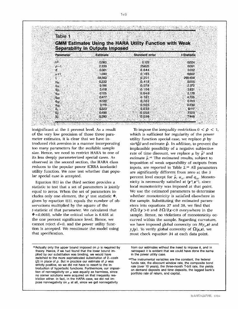
Table 1

GMM Estimates Using the HARA Utility Function with WeakSeparability in Outputs ImposedParameter Estimate Standard error f-Statistic

h 0.003 0.122 0.024p -1 2330 25.625 0.09 1d 0.001 0 044 0.012

1.090 0 165 6.60258382 0.201 2904590232 0418 0.555

q,. 0186 0.078 2372q21 0418 0 106 3.931q,1 0105 0.048 2178

0.477 0 101 4.7250120 0 162 0.743aiic 0.505 0.2300323 0.035 9.117

a? 0.436 0058 75230.280 0.038 7.448

insignificant at the 5 percent level. As a resultof the very low precision of those three para-meter estimates, it is clear that we have in-troduced risk aversion in a manner incorporatingtoo many parameters for the available samplesize. Hence, we need to restrict HARA to one ofits less deeply parameterized special cases. Asobserved in the second section, the HARA classreduces to the popular power (CRRA isoelastic)utility function. We now test whether that popu-lar special case is accepted.

Equation (61) in the third section provides astatistic to test that a set of parameters is jointlyequal to zeros. When the set of parameters in-cludes only one element, the x’ test statistic 0,given by equation (61), equals the number of ob-servations multiplied by the square of thet-statistic of that parameter. We calculated that0=0.0033, while the critical value is 6.635 atthe one percent significance level. Hence, wecannot reject d=0, and the power utility func-tion is accepted. We reestimate the model usingthat specification.

‘Tb impose the inequality restriction 0 < p < i,

which is sufficient for regularity of the powerutility function special case, we replace p bysin’(~)and estimate ~. In addition, to prevent theimplausible possibility of a negative subjectiverate of time discount, we replace ~zby ji’ andestimate ~L42 The estimated results, subject toimposition of weak separability of outputs frominputs, are reported in ‘Table 2.” All parametersare significantly different from zero at the 5percent level except for ~i, u,,, and q,,. Monoto-nicity is necessarily satisfied at (y’, xt), sincelocal monotonicity was imposed at that point.We use the estimated parameters to determinewhether monotonicity is satisfied elsewhere inthe sample. Substituting the estimated param-eters into equations 37 and 38, we find thatSQ/Sy>0 and SQ/Sx<o everywhere in thesample. Hence, no violations of monotonicity oc-curred within the sample. Regarding curvature,we have imposed global convexity on H(y0,x) andy0(y). lb verify global convexity of Q(y,x), wemust check equation 34 at each data point.

42Actually only the upper bound imposed on p is required bytheory. Hence, if we had found that the lower bound im-plied by our substitution was binding, we would haveswitched to the more sophisticated substitution of 2—cosh@) in place of p. But in practice our estimate of p wasstrictly positive, so we did not have to resort to the in-troduction of hyperbolic functions. Furthermore, our imposi-tion of nonnegativity on ~, was equally as harmless, sinceno corner solutions were acquired on that inequality res-triction either. In fact, in the HARA case, we did not im-pose nonnegativity on ,~at all, since we got nonnegativity

from our estimates without the need to impose it, and inretrospect it is evident that we could have done the samein the power utility case.

“The instrumental variables are the constant, the federalfunds rate, the discount window rate, the composite bondrate (over 10 years), the three-month T-bill rate, the yieldson demand deposits and time deposits, the lagged bank’sportfolio rate of return, and capital.

MARCH/APRiL 1994

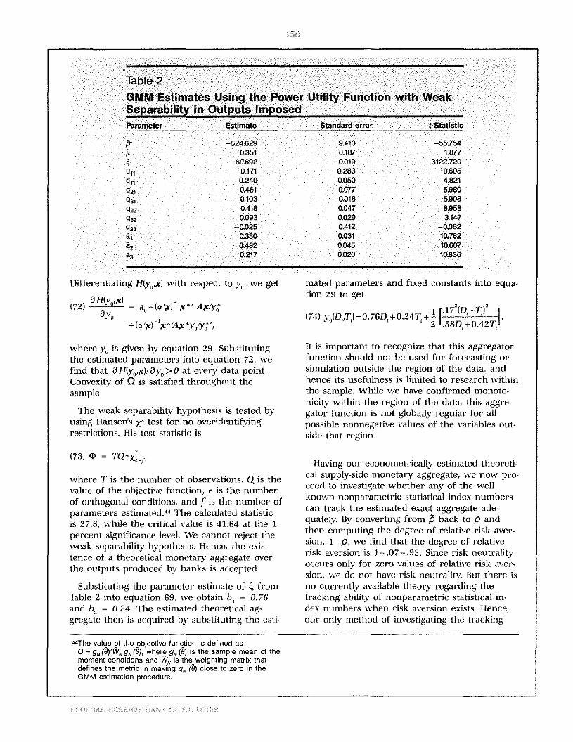
Table 2GMM Estimates Using the Power Utility Function with WeakSeparability in Outputs ImposedParameter Estimate Standard error f-Statistic

—524.629 9.410 —55.754ji 0351 0187 1877

60692 0.019 3122.720u1 0171 0.283 0.605

0.240 0.050 4.8210.461 0.077 5.9800.103 0.016 5.908

q22 0418 0.047 8.9580093 0029 3147

—0.025 0412 —0.062a 0.330 0031 10.762

0482 0045 10.6070.217 0020 10.836

Differentiating H(y,,y) with respect to y0, we get

(72) OH(y~x)= a0

_(atx)’y*T Ax/y

+(a~xY’x*/Ax*~v/w*2

where j’0

is given by equation 29. Substitutingthe estimated parameters into equation 72, wefind that QH(y,,x)I&y,>o at every data point.Convexity of C) is satisfied throughout thesample.

The weak separability hypothesis is tested byusing Hansen’s x’ test for no overidentifyingrestrictions. His test statistic is

CD =

where T is the number of observations, Q is thevalue of the objective function, e is the numberof orthogonal conditions, and f is the number ofparameters estimated.’~The calculated statisticis 27.6, while the critical value is 41.64 at the 1percent significance level. We cannot reject theweak separability hypothesis. Hence, the exis-tence of a theoretical monetary aggregate overthe outputs produced by banks is accepted.

Substituting the parameter estimate of t~.from‘Table 2 into equation 69, we obtain b, = 0.76and b, = 0.24. The estimated theoretical ag-gregate then is acquired by substituting the esti-

mated parameters and fixed constants into equa-tion 29 to get

1 i.17’W —T)’(74) y0(D,,T,)=0.76D,+0.24T,-i-— I ‘

2 t.58D,+o.42T,

It is important to recognize that this aggregatorfunction should not be used for forecasting orsimulation outside the region of the data, andhence its usefulness is limited to research withinthe sample. While we have confirmed monoto-nicity within the region of the data, this aggre-gator function is not globally regular for allpossible nonnegative values of the variables out-side that region.

Having our econometrically estimated theoreti-cal supply-side monetary aggregate, we now pro-ceed to investigate whether any of the wellknown nonparametric statistical index numberscan track the estimated exact aggregate ade-quately By converting from ~ back to p andthen computing the degree of relative risk aver-sion, 1— p, we find that the degree of relativerisk aversion is t— .07=93. Since risk neutralityoccurs only for zero values of relative risk aver-sion, we do not have risk neutrality But there isno currently available theory regarding thetracking ability of nonparametric statistical in-dex numbers when risk aversion exists. Hence,our only method of investigating the tracking

“The value of the objective function is defined asQ = g,(9)’W,g,(’6), where g,(6) is the sample mean of themoment conditions and WN is the weighting matrix thatdefines the metric in making gN (8) close to zero in theGMM estimation procedure.

151

ability of the more easily computed nonparamet-nc statistical indexes is to estimate the exact in-dex econometrically as we just have done, andcompare its behavior with that of the statisticalindex numbers.

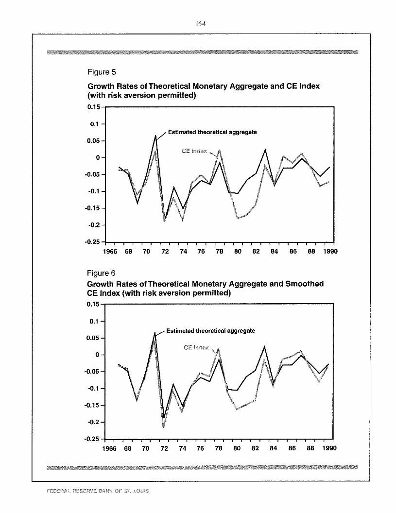
In this paper, we compare the estimated theo-retical aggregate with the Divisia, simple-sumand CE indexes. Rotemberg, Driscoll and Poterba(1991) have found that the growth rate of theCE index is very volatile with monthly data.Hence, they have proposed (see their footnote11) a method of smoothing that index’s growthrates by replacing the index’s weights by 13-month, centered moving averages. Since we areusing annual data, there already is a form ofsmoothing implicit in the data construction.Nevertheless, in addition to computing the annu-al contemporaneous CE index, we compute thesmoothed index in accordance with the methodselected by Rotemberg, Driscoll and Poterba.

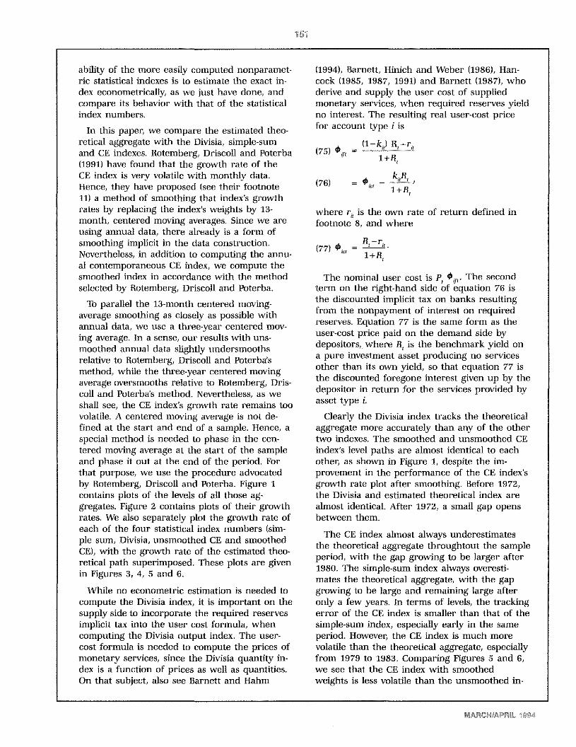
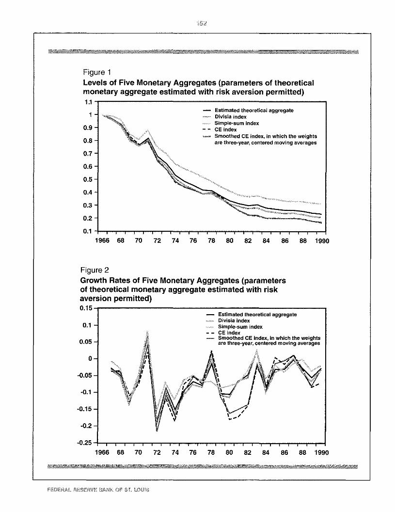
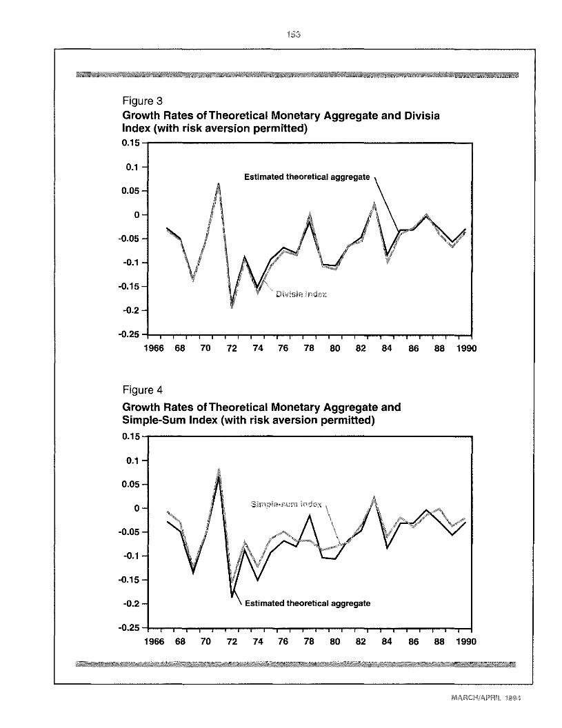
lb parallel the 13-month centered moving-average smoothing as closely as possible withannual data, we use a three-year centered mov-ing average. In a sense, our results with uns-moothed annual data slightly undersmoothsrelative to Rotemberg, Driscoll and Poterba’smethod, while the three-year centered movingaverage oversmooths relative to Rotemberg, Dris-coil and Poterba’s method. Nevertheless, as weshall see, the CE index’s growth rate remains toovolatile. A centered moving average is not de-fined at the start and end of a sample. Hence, aspecial method is needed to phase in the cen-tered moving average at the start of the sampleand phase it out at the end of the period. Forthat purpose, we use the procedure advocatedby Rotemberg, Driscoil and Poterba. Figure 1contains plots of the levels of all those ag-gregates. Figure 2 contains plots of their growthrates. We also separately plot the growth rate ofeach of the four statistical index numbers (sim-ple sum, Divisia, unsmoothed CE and smoothedCE), with the growth rate of the estimated theo-retical path superimposed. These plots are givenin Figures 3, 4, 5 and 6.

While no econometric estimation is needed tocompute the Divisia index, it is important on thesupply side to incorporate the required reservesimplicit tax into the user cost formula, whencomputing the Divisia output index. The user-cost formula is needed to compute the prices ofmonetary services, since the Divisia quantity in-dex is a function of prices as well as quantities.On that subject, also see Barnett and Hahm

(1994), Barnett, Hinich and Weber (1986), Han-cock (1985, 1987, 1991) and Barnett (1987), whoderive and supply the user cost of suppliedmonetary services, when required reserves yieldno interest. The resulting real user-cost pricefor account type i is

(1—k.) H —r.

1+R,

k.B(76) = 0~,—

1+11,

where r, is the own rate of return defined infootnote 8, and where

=

(77) °~ 1 + B,

The nominal user cost is P, 0~.The secondterm on the right-hand side of equation 76 isthe discounted implicit tax on banks resultingfrom the nonpayment of interest on requiredreserves. Equation 77 is the same form as theuser-cost price paid on the demand side bydepositors, where B, is the benchmark yield ona pure investment asset producing no servicesother than its own yield, so that equation 77 isthe discounted foregone interest given up by thedepositor in return for the services provided byasset type i.

Clearly the Divisia index tracks the theoreticalaggregate more accurately than any of the othertwo indexes. The smoothed and unsmoothed CEindex’s level paths are almost identical to eachother, as shown in Figure 1, despite the im-provement in the performance of the CE index’sgrowth rate plot after smoothing. Before 1972,the Divisia and estimated theoretical index arealmost identical. After 1972, a small gap opensbetween them.

The CE index almost always underestimatesthe theoretical aggregate throughtout the sampleperiod, with the gap growing to be larger after1980. The simple-sum index always overesti-mates the theoretical aggregate, with the gapgrowing to be large and remaining large afteronly a few years. In terms of levels, the trackingerror of the CE index is smaller than that of thesimple-sum index, especially early in the sameperiod. However, the CE index is much morevolatile than the theoretical aggregate, especiallyfrom 1979 to 1983. Comparing Figures 5 and 6,we see that the CE index with smoothedweights is less volatile than the unsmoothed in-

MARCH/APRIL 1994

152

Figure 1Levels of Five Monetary Aggregates (parameters of theoreticalmonetary aggregate estimated with risk aversion permitted)ii

1—

0.9 -

0.8 -

0,7 -

0-6 -

0.5 -

0.4 -

0.3-

0.2 -

01

1966

Figure 2Growth Rates of Five Monetary Aggregates (parametersof theoretical monetary aggregate estimated with riskaversion permitted)0.15

0.1

0.05 -

0-

-0.05 -

-0.1 -

-0.15-

-0.2 -

-0.25

— Estimated theoretical aggregateDivisia indexSimple-sum index

— — CE indexSmoothed CE index, in which the weightsare three-year, centered moving averages

I I I I

68 70 72 74 76 78 80 82 84 86 88 1990

— Estimated theoretical aggregateDivisia indexSimple-sum index

— — CE index— Smoothed CE index, in which the weights

are three-year, centered moving averages

1966I I I I I I

68 70 72 74 76 78 80 82 84 86 88 1990

FEDERAL RESERVE BANK OF ST. LOUIS

153

Figure 3Growth Rates of Theoretical Monetary Aggregate and DivisiaIndex (with risk aversion permitted)0.15

0.1 -

0-05 -

0-

-0-05 -

—0.1 -

-0.15-

-0.2 -

-0.25

1966

Figure 4

Growth Rates of Theoretical Monetary Aggregate andSimple-Sum Index (with risk aversion permitted)0,15-

0-1 -

0.05 -

0-

-0-05 -

-0.1 -

-0.15-

-0-2 -

-0.25

1966

Estimated theoretical aggregate

Divisia index

I I I I I I I I I I I I I I I I I I I I

68 70 72 74 76 78 80 82 84 86 88 1990

Simpie-surn index

Estimated theoretical aggregate

I I I I I I I I I I I I I I I I I I J I

68 70 72 74 76 78 80 82 84 86 88 1990

MARCH/APRIL 1994

154

Figure 5

Growth Rates of Theoretical Monetary Aggregate and CE Index(with risk aversion permitted)

1966

Figure 6Growth Rates of Theoretical Monetary AggregateCE Index (with risk aversion permitted)

1966

and Smoothed

1990

0.15

0.1 -

Estimated theoretical aggregate

0.05 -

0-

-0.05 -

-0.1 -

-0.15-

-0.2 -

-0.25 I I I I I I I I I I I I I I I I $ I I $ I I I

68 70 72 74 76 78 80 82 84 86 88 1990

015

0.1 -

Estimated theoretical aggregate0.05-

0-

-0.05 -

—0.1 -

-0.15-

-0.2 -

-0.25

68 70 72 74 76 78 80 82 84 86 88

FEDERAL RESERVE BANK OF ST. LOUiS

155

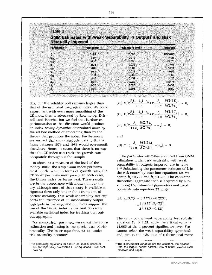
Table 3GMM Estimates with Weak Separability in Outputs and RiskNeutrality ImposedParameter Estimate Standard error t-Statistic

61 82 0.005 11968.80u. 0.27 0019 1431q.- 018 0.005 32.78q21 0.38 0022 17.01

0.07 0.007 10140.44 0.023 19.090.11 0063 1.66

q33 a16 0.132 1 250.33 0.002 16274050 0003 16439023 0006 3650

dex, but the volatility still remains larger thanthat of the estimated theoretical index. We couldexperiment with even more smoothing of theCE index than is advocated by Rotemberg, Dris-coll, and Poterba, but we feel that further ex-perimentation in that direction would producean index having dynamics determined more bythe ad hoc method of smoothing than by thetheory that produces the index. Furthermore,we suspect that smoothing adequate to fix theindex between 1979 and 1983 would oversmoothelsewhere. Hence, it seems that there is no waythat the CE index can track the growth ratesadequately throughout the sample.

In short, as a measure of the level of themoney stock, the simple-sum index performsmost poorly, while in terms of growth rates, theCE index performs most poorly. In both cases,the Divisia index performs best. These resultsare in the accordance with index number the-ory although most of that theory is available inrigorous form only under the assumption ofperfect certainty. Our weak separability test sup-ports the existence of an inside-money outputaggregate in banking, and our plots support theuse of the Divisia index as the best currentlyavailable statistical index for tracking that out-put aggregate.

For comparison purposes, we repeat the aboveestimation and testing in the special case of riskneutrality. The Euler equations, 62-65, underrisk neutrality become~’

11(1—k )—r B 00./3D(78) E{P ‘ “ “-i-P ‘ I] = 0,

‘1+11, 30/ac,

(79) 11{p~1kzI)rZ~~pB, 00/aT, =1+11, ‘1+11, 30/0C,

B 30/3L(80) UP,—’— aoiac~—w,,} = 0,

and

B 30/dM(81)E[P ‘ ‘ —w] = o.‘l+B, 30./ac,

The parameter estimates acquired from GMMestimation under risk neutrality, with weakseparability in outputs imposed, are in table346 Substituting the parameter estimate of ~ inthe risk-neutrality case into equations 69, weobtain b,=0.777 and b2=0.223. The estimatedtheoretical aggregate then is acquired by sub-stituting the estimated parameters and fixedconstants into equation 29 to get

(82) y,JD,,T,) = 0.777D,+O.223T,

~-_ [.275W1_T~) -2 t.58D,+0.427

The value of the weak separability test statistic,equation 73, is 9.25, while the critical value is21.666 at the 1 percent significance level. Wecannot reject the weak separability hypothesisand, hence, the existence of a theoretical mone-

45ln producing equations 80 and 81 as special cases ofthe corresponding risk-averse Euler equations, recall foot-note 14.

~The instrumental variables are the constant, the discountrate, the lagged banks’ portfolio rate of return, excess cashreserves and capital.

MARCH/APRiL 1994

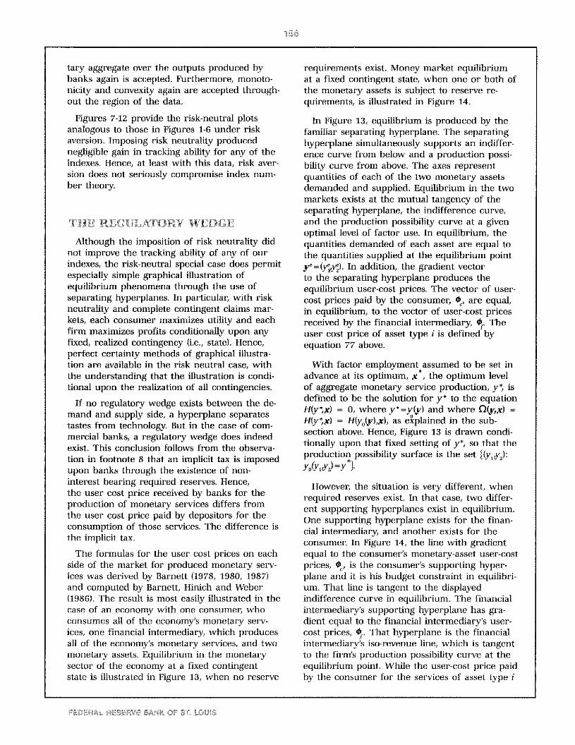
156

tary aggregate over the outputs produced bybanks again is accepted. Furthermore, monoto-nicity and convexity again are accepted through-out the region of the data.

Figures 7-12 provide the risk-neutral plotsanalogous to those in Figures 1-6 under riskaversion. Imposing risk neutrality producednegligible gain in tracking ability for any of theindexes. Hence, at least with this data, risk aver-sion does not seriously compromise index num-ber theory

¶1711E RE(II.JL.XI1)RY ‘WEDGE

Although the imposition of risk neutrality did

not improve the tracking ability of any of ourindexes, the risk-neutral special case does permitespecially simple graphical illustration ofequilibrium phenomena through the use ofseparating hyperplanes. In particular, with riskneutrality and complete contingent claims mar-kets, each consumer maximizes utility and eachfirm maximizes profits conditionally upon anyfixed, realized contingency (i.e., state). Hence,perfect certainty methods of graphical illustra-tion are available in the risk neutral case, withthe understanding that the illustration is condi-tional upon the realization of all contingencies.

If no regulatory wedge exists between the de-mand and supply side, a hyperplane separatestastes from technology. But in the case of com-mercial banks, a regulatory wedge does indeedexist. This conclusion follows from the observa-tion in footnote 8 that an implicit tax is imposedupon banks through the existence of non-interest bearing required reserves. Hence,the user cost price received by banks for theproduction of monetary services differs fromthe user cost price paid by depositors for theconsumption of those services. The difference isthe implicit tax -

The formulas for the user cost prices on eachside of the market for produced monetary serv-ices was derived by Barnett (1978, 1980, t987)and computed by Barnett, Hinich and Weber(1986). The result is most easily illustrated in thecase of an economy with one consumer, whoconsumes all of the economy’s monetary serv-ices, one financial intermediary, which producesall of the economy’s monetary services, and twomonetary assets. Equilibrium in the monetarysector of the economy at a fixed contingentstate is illustrated in Figure 13, when no reserve

requirements exist. Money market equilibriumat a fixed contingent state, when one or both ofthe monetary assets is subject to reserve re-quirements, is illustrated in Figure 14.

In Figure 13, equilibrium is produced by thefamiliar separating hyperplane. The separatinghyperplane simultaneously supports an indiffer-ence curve from below and a production possi-bility curve from above. The axes representquantities of each of the two monetary assetsdemanded and supplied. Equilibrium in the twomarkets exists at the mutual tangency of theseparating hyperplane, the indifference curve,and the production possibility curve at a givenoptimal level of factor use. In equilibrium, thequantities demanded of each asset are equal tothe quantities supplied at the equilibrium point

= (y~,,y~)- In addition, the gradient vectorto the separating hyperplane produces theequilibrium user-cost prices. The vector of user-cost prices paid by the consumer, O~,are equal,in equilibrium, to the vector of user-cost pricesreceived by the financial intermediary, ¶ Theuser cost price of asset type i is defined byequation 77 above.

With factor employment assumed to be set inadvance at its optimum, xt, the optimum levelof aggregate monetary service production, y ~, isdefined to be the solution for y~to the equationH(y’~x)= 0, where y~=y(y) and where O(j~x)=H(y*,x) = H(y0(yLx), as e&plained in the sub-section above. Hence, Figure 13 is drawn condi-tionally upon that fixed setting of y~,so that theproduction possibility surface is the set

y0(y,,y2) =yt}-

However, the situation is very different, whenrequired reserves exist. In that case, two differ-ent supporting hyperplanes exist in equilibrium.One supporting hyperplane exists for the finan-cial intermediary, and another exists for theconsumer. In Figure 14, the line with gradientequal to the consumer’s monetary-asset user-costprices, 4~,is the consumer’s supporting hyper-plane and it is his budget constraint in equilibri-um. That line is tangent to the displayedindifference curve in equilibrium. The financialintermediary’s supporting hyperplane has gra-dient equal to the financial intermediary’s user-cost prices, ‘~. That hyperplane is the financialintermediary’s iso-revenue line, which is tangentto the firm’s production possibility curve at theequilibrium point. While the user-cost price paidby the consumer for the services of asset type i

FED ER-A L RESERVS SANK OF St LOUiS

1-57

Figure 7Levels of Five Monetary Aggregates (parameters of theoreticalmonetary aggregate estimated with imposed risk neutrality)

0-9 -

0.8 -

0.7 -

0.6 -

0.5 -

0,4 -

0,3 -

0.2 -

0.1 -

Figure 8Growth Rates of Five Monetary Aggregates (parametersof theoretical monetary aggregate estimated subjectto imposed risk neutrality)

0.05-

0-

-0M5 -

-0_I -

-0.15-

-0.2-

-0.25 -

1966 68 70 72 74 76 78 80 82 84 86 88

1990

1990

1,1

1— Estimated theoretical aggregate-~ Divisia index

Simple-sum index— — CE index— Smoothed CE index, in which the weights

are three-year, centered moving averages

I I~I $ I I1 I I~rI II~t I I I I I I I I

1966 68 70 72 74 76 78 80 82 84 86 88

0.15

0.1 -

Estimated theoretical aggregateDivisia indexSimple-sum indexCE indexSmoothed CE index, in which the weightsare three-year, centered moving averages

I I

MARCH/APRiL 1994

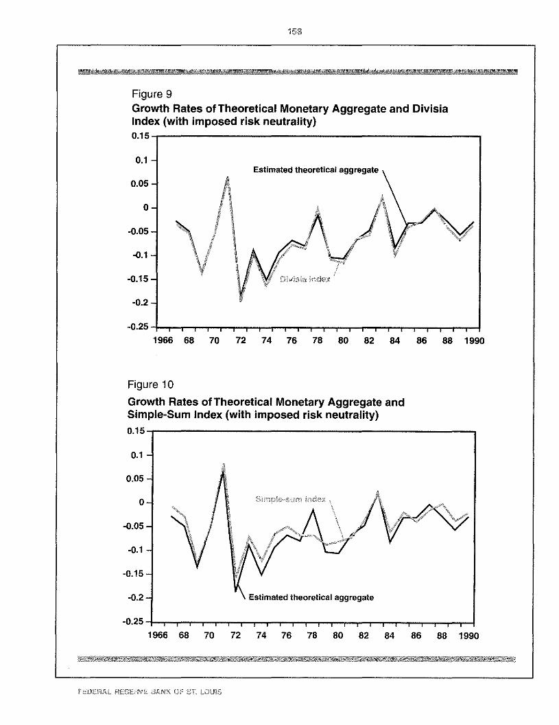
158

Figure 9Growth Rates of Theoretical Monetary Aggregate and DivisiaIndex (with imposed risk neutrality)

Growth Rates of Theoretical Monetary Aggregate andSimple-Sum Index (with imposed risk neutrality)0.15-

I I I r I

86 88 1990

0.15

0.1Estimated theoretical aggregate

0.05 -

0—

-0.05 -

-0_i -

-0.15

-0.2 -

-0.25

1966

Figure 10

I I I I

68 70 72 74 76 78 80 82 84 86 88 1990

Simpie-sun~index

0.1 -

0_os -

0-

-0.05 -

-0_i -

-0.15-

-0.2 -

-0.25

1966

Estimated theoretical aggregate

I I I I I I I I I I I I I I I I I

68 70 72 74 76 78 80 82 84

FEDERAL RESERVE SANK OF ST. LOWS

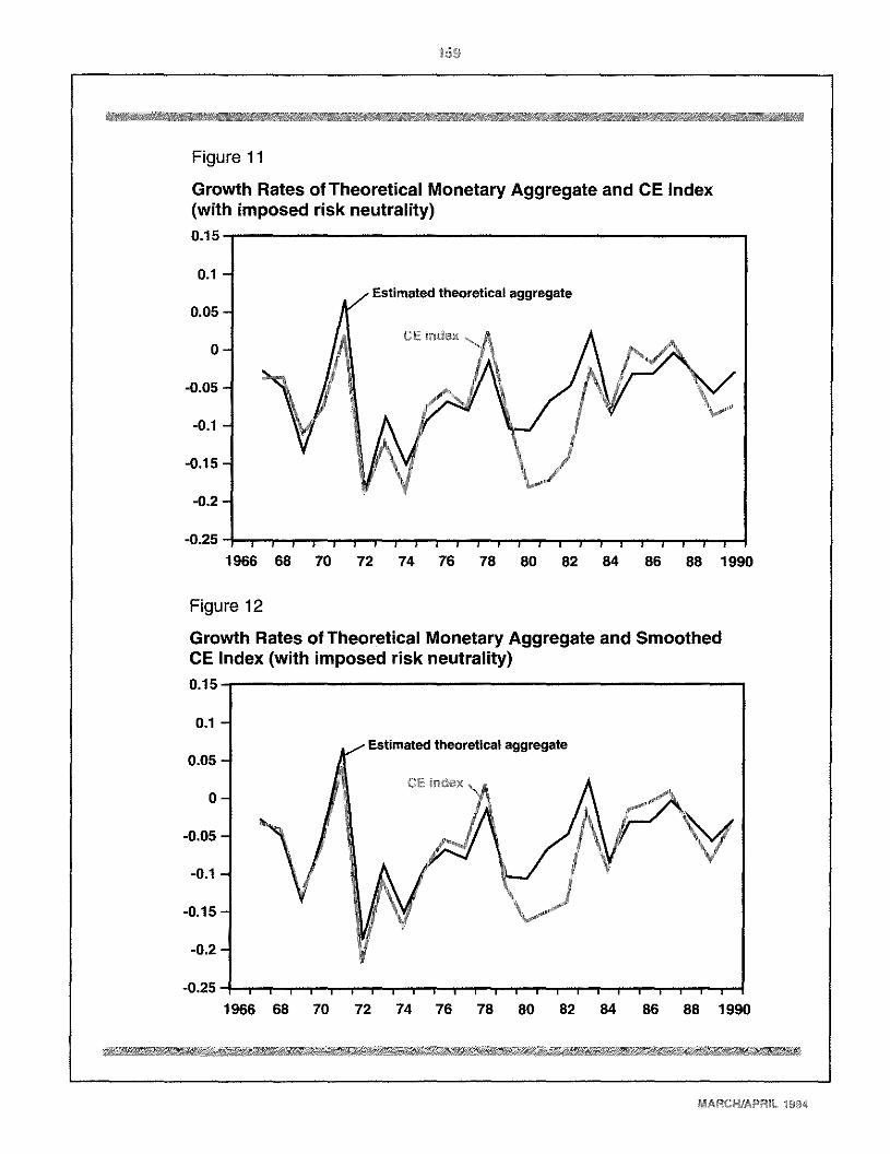
159

Figure 11

Growth Rates of Theoretical Monetary Aggregate and CE Index(with imposed risk neutrality)

1966

Figure 12

Growth Rates of Theoretical Monetary AggregateCE Index (with imposed risk neutrality)

1966

and Smoothed

0.15

0.1 -

Estimated theoretical aggregate0.05-

0-

-0.05 -

-0.1 -

-0.15-

-0.2 -

-0.25 I I I I I I I I I I I I I I I I I I I I I I

68 70 72 74 76 78 80 82 84 86 88 1990

0.15

0,1 -

Estimated theoretical aggregate0.05 -

0-

-0_os -

-0.1 -

-0.15-

-0.2 -

-0.25

68 70 72 74 76 78 80 82 84 86 88 1990

MARCH/APRfL 1994

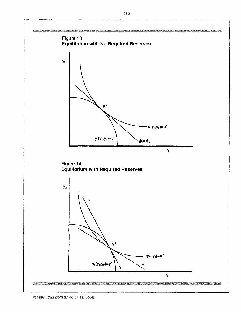
160

Figure 13Equilibrium with No Required Reserves

Y2

Figure 14Equilibrium with Required Reserves

Y2

ye

ye

Vi

FEOERAL RESERVE BANK OF ST. LOWS

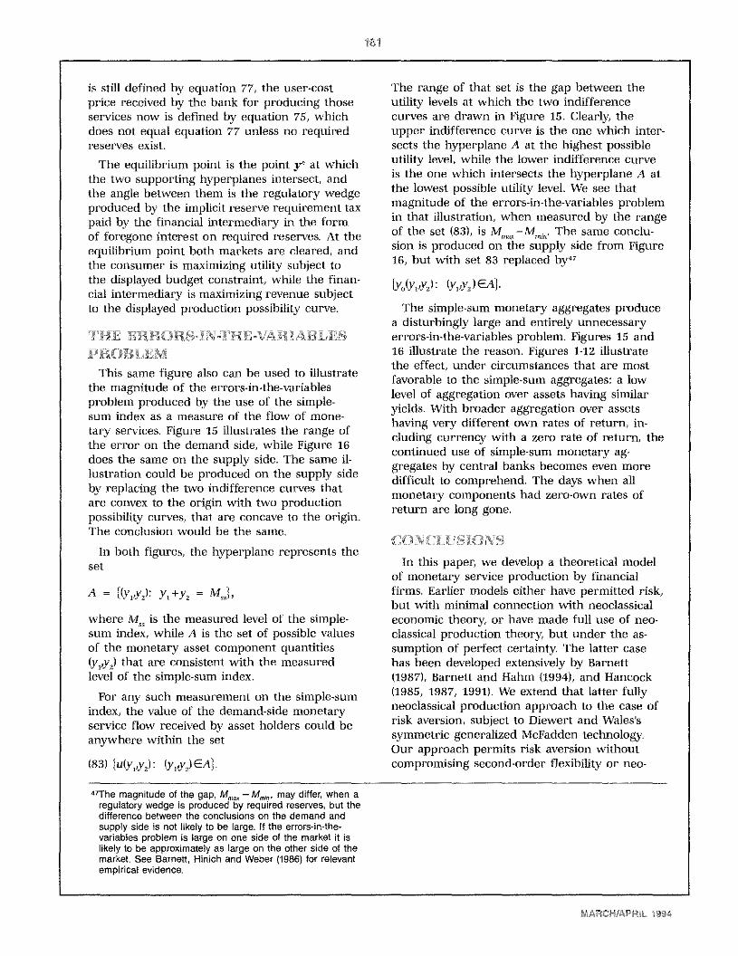
161

is still defined by equation 77, the user-costprice received by the bank for producing thoseservices now is defined by equation 75, whichdoes not equal equation 77 unless no requiredreserves exist.

The equilibrium point is the point y at whichthe two supporting hyperplanes intersect, andthe angle between them is the regulatory wedgeproduced by the implicit reserve requirement taxpaid by the financial intermediary in the formof foregone interest on required reserves. At theequilibrium point both markets are cleared, andthe consumer is maximizing utility subject tothe displayed budget constraint, while the finan-cial intermediary is maximizing revenue subjectto the displayed production possibility curve.

rfijf, EDRORS-iN~FHE-VA.Ri/%B.LE-S

EL OR LEM

This same figure also can be used to illustratethe magnitude of the errors-in-the-variablesproblem produced by the use of the simple-sum index as a measure of the flow of mone-tary services. Figure 15 illustrates the range ofthe error on the demand side, while Figure 16does the same on the supply side. The same il-lustration could be produced on the supply sideby replacing the two indifference curves thatare convex to the origin with two productionpossibility curves, that are concave to the origin.The conclusion would be the same.

In both figures, the hyperplane represents the

set

A = {(y,,y): y1+y~= M,j,

where is the measured level of the simple-sum index, while A is the set of possible valuesof the monetary asset component quantities(y,,y

2) that are consistent with the measured

level of the simple-sum index.

For any such measurement on the simple-sumindex, the value of the demand-side monetaryservice flow received by asset holders could beanywhere within the set

(83) {u(y,,y): (y1,y)EA}.

The range of that set is the gap between theutility levels at which the two indifferencecurves are drawn in Figure 15. Clearly, theupper indifference curve is the one which inter-sects the hyperplane A at the highest possibleutility level, while the lower indifference curveis the one which intersects the hyperplane A atthe lowest possible utility level. We see thatmagnitude of the errors-in-the-variables problemin that illustration, when measured by the rangeof the set (83), is ~ The same conclu-sion is produced on the supply side from Figure16, but with set 83 replaced by47

{y,(y1,y~): (y,,y,)EA}.

The simple-sum monetary aggregates producea disturbingly large and entirely unnecessaryerrors-in-the-variables problem. Figures 15 and16 illustrate the reason. Figures 1-12 illustratethe effect, under circumstances that are mostfavorable to the simple-sum aggregates: a lowlevel of aggregation over assets having similaryields. With broader aggregation over assetshaving very different own rates of return, in-cluding currency with a zero rate of return, thecontinued use of simple-sum monetary ag-gregates by central banks becomes even moredifficult to comprehend. The days when allmonetary components had zero-own rates ofreturn are long gone.

In this paper, we develop a theoretical modelof monetary service production by financialfirms. Earlier models either have permitted risk,but with minimal connection with neoclassicaleconomic theory or have made full use of neo-classical production theory but under the as-sumption of perfect certainty. The latter casehas been developed extensively by Barnett(1987), Barnett and Hahm (1994), and Hancock(1985, 1987, 1991). We extend that latter fullyneoclassical production approach to the case ofrisk aversion, subject to Diewert and Wales’ssymmetric generalized McFadden technology.Our approach permits risk aversion withoutcompromising second-order flexibility or neo-

47The magnitude of the gap, Mms, — Mmm, may differ, when aregulatory wedge is produced by required reserves, but thedifference between the conclusions on the demand andsupply side is not likely to be large. If the errors-in-the-variables problem is large on one side of the market it islikely to be approximately as large on the other side of themarket. See Barnett, Hinich and Weber (1986) for relevantempirical evidence.

MARCH/APRiL 1994

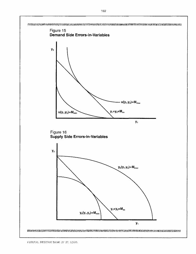
162

Figure 15Demand Side Errors-in-Variables

ViFigure 16

Supply Side Errors-in-Variables

V2

Vi

FEOERAL RESERVE BANK OF ST LOUIS

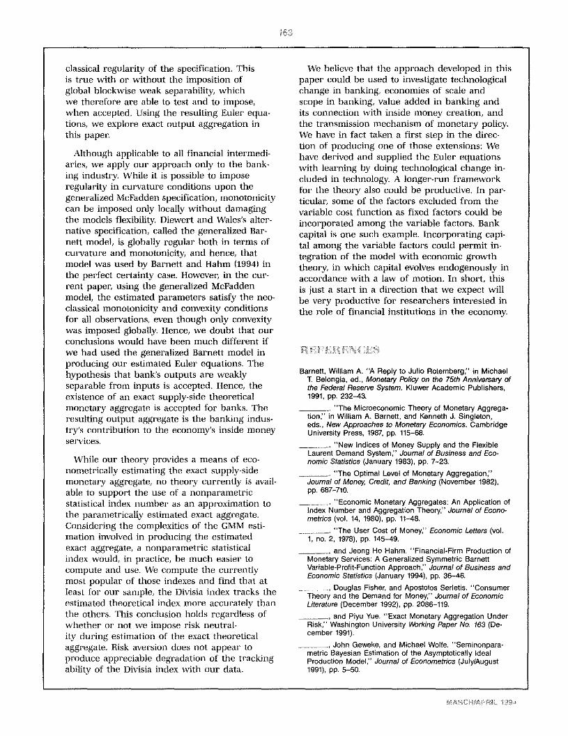
163

classical regularity of the specification. Thisis true with or without the imposition ofglobal blockwise weak separability whichwe therefore are able to test and to impose,when accepted. Using the resulting Euler equa-tions, we explore exact output aggregation inthis paper.

Although applicable to all financial intermedi-aries, we apply our approach only to the bank-ing industry While it is possible to imposeregularity in curvature conditions upon thegeneralized McFadden specification, monotonicitycan be imposed only locally without damagingthe models flexibility. Diewert and Wales’s alter-native specification, called the generalized Bar-nett model, is globally regular both in terms ofcurvature and monotonicity and hence, thatmodel was used by Barnett and Hahm (1994) inthe perfect certainty case. However, in the cur-rent paper, using the generalized McFaddenmodel, the estimated parameters satisfy the neo-classical monotonicity and convexity conditionsfor all observations, even though only convexitywas imposed globally. Hence, we doubt that ourconclusions would have been much different ifwe had used the generalized Barnett model inproducing our estimated Euler equations, Thehypothesis that bank’s outputs are weaklyseparable from inputs is accepted. Hence, theexistence of an exact supply-side theoreticalmonetary aggregate is accepted for banks. Theresulting output aggregate is the banking indus-try’s contribution to the economy’s inside moneyservices.

While our theory provides a means of eco-nometrically estimating the exact supply-sidemonetary aggregate, no theory currently is avail-able to support the use of a nonparametricstatistical index number as an approximation tothe parametrically estimated exact aggregate.Considering the complexities of the GMM esti-mation involved in producing the estimatedexact aggregate, a nonparametric statisticalindex would, in practice, be much easier tocompute and use. We compute the currentlymost popular of those indexes and find that atleast for our sample, the Divisia index tracks theestimated theoretical index more accurately thanthe others. This conclusion holds regardless ofwhether or not we impose risk neutral-ity during estimation of the exact theoreticalaggregate. Risk aversion does not appear toproduce appreciable degradation of the trackingability of the IJivisia index with our data.

We believe that the approach developed in thispaper could be used to investigate technologicalchange in banking, economies of scale andscope in banking, value added in banking andits connection with inside money creation, andthe transmission mechanism of monetary policyWe have in fact taken a first step in the direc-tion of producing one of those extensions: Wehave derived and supplied the Euler equationswith learning by doing technological change in-cluded in technology. A longer-run frameworkfor the theory also could be productive. Jn par-ticular, some of the factors excluded from thevariable cost function as fixed factors could beincorporated among the variable factors. Bankcapital is one such example. Incorporating capi-tal among the variable factors could permit in-tegration of the model with economic growththeory in which capital evolves endogenously inaccordance with a law of motion. In short, thisis just a start in a direction that we expect willbe very productive for researchers interested inthe role of financial institutions in the economy

Barnett, William A. “A Reply to Julio Rotemberg,” in MichaelT. Belongia, ed., Monetary Palky on the 75th Anniversary ofthe Federal Reserve System. Kluwer Academic Publishers,1991, pp. 232—43.

_______ “The Microeconomic Theory of Monetary Aggrega-tion,” in William A. Barnett, and Kenneth J. Singleton,eds., New Approaches to Monetary Economics. CambridgeUniversity Press, 1987, pp. 115—68.

_______- “New Indices of Money Supply and the FlexibleLaurent Demand System,” Journal of Business and Eco-nomic Statistics (January 1983), pp. 7—2a

_______ “The Optimal Level of Monetary Aggregation:’Journal of Money, Credit, and Banking (November 1982),pp. 687—710.

______ “Economic Monetary Aggregates: An Application ofIndex Number and Aggregation Theory,” Journal of Econo-metrics (vol. 14, 1980), pp. 11—4&

_______ “The User Cost of Money,” Economic Letters (vol.1, no. 2, 1978), pp. 145—49.

______ and Jeong Ho Hahm. “Financial-Firm Production ofMonetary Services: A Generalized Symmetric BarnettVariable-Prof it-Function Approach’ Journal of Business andEconomic Statistics (January 1994), pp. 36—46.

Douglas Fisher, and Apostolos Serletis. “ConsumerTheory and the Demand for Money,” Journal of EconomicLiterature (December 1992), pp. 2086—119.

_______ and Piyu Vue. “Exact Monetary Aggregation UnderRisk,” Washington University Working Paper No. 163 (De-cember 1991).

_______ John Geweke, and Michael Wolfe. “Seminonpara-metric Bayesian Estimation of the Asymptotically IdealProduction ModeL” Journal of Econometrics (July/August1991), pp. 5—50.

MARCH/APRIL 1-994

16-4

_______ Melvin J. Hinich and Warren E. Weber. “TheRegulatory Wedge Between the Demand-Side and Supply-Side Aggregation-Theoretic Monetary Aggregates,” Journalof Econometrics (October/November 1986), pp. 165—85.

_______ and Yul W. Lee. “The Global Properties of the Mm-flex Laurent, Generalized Leontief, and Translog FlexibleFunctional Forms,” Econometrica (November 1985), pp.1421 —37.

_______ Edward K. Offenbacher, and Paul A. Spindt. “TheNew Divisia Monetary Aggregates:’ Journal of PoliticalEconomy (December 1984), pp. 1049—85.

Belongia, Michael t, and James A. Chalfant. “The ChangingEmpirical Definition of Money: Some Estimates from aModel of the Demand for Money Substitutes:’ Journal ofPolitical Economy (April 1989), pp. 387—97.

Bernanke, Ben, and Mark Gertler. “Banking and Macroeco-nomic Equilibrium’ in William A. Barnett, and Kenneth J.Singleton, eds., New Approaches to Monetary Economics.Cambridge University Press, 1987, pp. 89—111.

Bhattacharya, Sudipto, and Douglas Gale. “PreferenceShocks, Liquidity, and Central Bank Policy,” in William A.Barnett, and Kenneth J. Singleton, eds., New Approachesto Monetary Economics. Cambridge University Press, 1987,pp. 69—88.

Blackorby, Charles, William Schworm, and Timothy Fisher.“Testing for the Existence of Input Aggregates in an Econ-omy Production Function:’ University of British ColumbiaDiscussion Paper No. 86-26 (1986).

_______ Daniel Primont, and R. Robert Russell. “On Test-ing Separability Restrictions with Flexible FunctionalForms,” Journal of Econometrics (March 1977), pp. 195—209.

Brainard, William, and James Tobin. “Pitfalls in FinancialModel Building:’ The American Economic Review (May1968, Papers and Proceedings 1967), pp. 99—122.

_______ “Financial Intermediaries and the Effectiveness ofMonetary Controls:’ The American Economic Review (May1963, Papers and Proceedings 1962), pp. 383—400.

Brown, Randall S., Douglas W. Caves, and Laurits R.Christensen. “Modeling the Structure of Cost and Produc-tion for Multiproduct Firms:’ Southern Economic Journal(July 1979), pp. 256—73.

Debreu, Gerard. Theory of Value, An Axiomatic Analysis ofEconomic Equilibrium, Cowles Foundation Monograph 17,Yale University Press, 1959.

Denny, Michael, and Melvyn Fuss. “The Use of Approxima-tion Analysis to Test for Separability and Existence of Con-sistent Aggregates,” The American Economic Review (June1977), pp. 404—18.

Diamond, Douglas W., and Phillip H. Dybvig. “Bank Runs,Deposit Insurance, and Liquidity:’ Journal of Political Econ-omy (June 1983), pp. 401—19.

Diewert, W. E. “Exact and Superlative Index Numbers:’ Jour-nal of Econometrics (May 1976), pp. 115—45.

________- “Functional Forms for Profit and TransformationFunctions,” Journal of Economic Theory (June 1973), pp.284—316.

_______ “An Application of the Shephard Duality Theorem:A Generalized Leontief Production Function,” Journal of Pa-litical Economy (May/June 1971), pp. 481—507.

_______ and T,J. Wales. “Flexible Functional Forms andTests of Homogeneous Separability:’ University of BritishColumbia Discussion Paper Na 91-12 (1991).

_______ “A Normalized Quadratic Semiflexible FunctionalForm,” Journal of Econometrics (March 1988), pp. 327—42.

_______ “Flexible Functional Forms and Global CurvatureConditions,” Econometrica (January 1987), pp. 43—68.

Duffie, Darrell. “The Theory of Value in Security Markets:’ inWerner Hildenbrand, and Hugo Sonnenschein, eds., Hand-book of Mathematical Economics, vol. IV. North-Holland,1991.

Gallant, A. Ronald. “Unbiased Determination of ProductionTechnologies’ Journal of Econometrics (vol. 20, 1982),pp. 2B5—a2a

“On the Bias in Flexible Functional Forms and anEssentially Unbiased Form: The Fourier Flexible Form:’Journal of Econometrics (vol. 15, 1981), pp. 211—45.

_______ and Gene H. Golub. “Imposing Curvature Restric-tions on Flexible Functional Forms,” Journal of Economet-rics (December 1984), pp. 295—321.

Hall, Robert E. “The Specification of Technology with SeveralKinds of OutpuL” Journal of Political Economy (July/August1973), pp. 878—92.

Hancock, Diana. A Theory of Production for the FinancialFirm. Kluwer Academic Publishers, 1991.

“Aggregation of Monetary Goods: A ProductionModel,” in William A. Barnett, and Kenneth J. Singleton,eds., New Approaches to Monetary Economics, CambridgeUniversity Press, 1987, pp. 200-18.

_______- “The Financial Firm: Production with Monetary andNonmonetary Goods:’ Journal of Political Economy (Oc-tober 1985), pp. 859-80.

Hansen, Lars Peter. “Large Sample Properties of GeneralizedMethod of Moments Estimators,” Econometrica (July 1982),pp. 1029—54.

_______ and Kenneth J. Singleton. “Generalized Instrumen-tal Variable Estimation of Nonlinear Rational ExpectationsModels:’ Econometrica (September 1982), pp. 1269—86.

Ingersoll, Jonathan E. Theory of Financial Decision Making.Rowman and Littlefield Publishers, Inc., 1987.

Jacklin, Charles J., and Sudipto Bhattacharya. “Distinguish-ing Panics and Information-Based Bank Runs: Welfare andPolicy Implications,” Journal of Political Economy (June1988), pp. 568—92.

Lau, L. J. “Testing and Imposing Monotonicity, Convexity andQuasi-Convexity Constraints,” in Melvyn Fuss, and DanielMcFadden, eds., Production Economics: A Dual Approachto Theory and Application. North-Holland, 1978, pp. 409—53.

Leontief, Wassily. “Introduction to a Theory of the InternalStructure of Functional Relationships,” Econometrica (Oc-tober 1947a), pp. 361—73.

_______ “A Note On The Interrelation Of Subsets Of In-dependent Variables Of A Continuous Function With Con-tinuous First Derivatives:’ Bulletin of the AmericanMathematical Society (April 1947b), pp. 343—50.

Mackinlay, A. Craig, and Matthew P. Richardson, “UsingGeneralized Method of Moments to Test Mean-Variance Ef-ficiency:’ Journal of Finance (June 1991), pp. 511—27.

Magill, Michael, and Wayne Shafer. “Incomplete Markets,” inWerner Hildenbrand and Hugo Sonnenschemn, eds,, Hand-book of Mathematical Economics, vol. IV, North-Holland,1991.

Newey, Whitney K., and Kenneth D. West. “A Simple, PositiveSemi-Definite, Heteroskedasticity and Autocorrelation Con-sistent Covariance Matrix:’ Econometrica (May 1987),pp. 703—08.

Poterba, James M., and Julio J. Rotemberg. “Money in theUtility Function: An Empirical Implementation:’ in WilliamA. Barnett, and Kenneth J. Singleton, eds., New Approachesto Monetary Economics. Cambridge University Press, 1987,pp. 219—40.

FEDERAL RESEP;VE BANK O-FST. LOU-IS

165

Robles, Barbara J. “The Optimal Demand for Money in U.S.Manufacturing: A Dynamic Micro Theoretic Approach,”University of Colorado at Boulder Discussion Paper No,93—15 (June 1993).

Rotemberg, Julio J. “Monetary Aggregates and Their Uses,”in Michael T. Belongia, ed., Monetary Policy on the 75thAnniversary of the Federal Reserve System. Kluwer Aca-demic Publishers, 1991, pp. 223—31.

_______ John C. Driscoll, and James Poterba, “Money, Out-put, and Prices: Evidence from a New Monetary Ag-gregate,” NBER Working Paper Na 3824 (August 1991).

Sargent, Thomas J. Dynamic Macroeconomic Theory. HarvardUniversity Press, 1987.

Swofford, James L., and Gerald A. Whitney. “NonparametricTests of Utility Maximization and Weak Separability forConsumption, Leisure, and Money:’ Review of Economicsand Statistics (August 1987), pp. 458—64.

Thornton, Daniel L,, and Piyu Yue, “An Extended Seriesof Divisia Monetary Aggregates:’ this Review(NovemberlDecember 1992), pp. 35—52.

Tobmn, James, “Money, Capital, and Other Stores ofValue’ The American Economic Review (May 1961),pp. 26—46.

Woodland, Alan D. “On Testing Weak Separability,” Journal ofEconometrics (December 1978), pp. 383—98.

MARCH/APRiL 199-4