Financial distress, bankruptcy law and the business cycle …suarez/suarez-sussman.pdf · ·...
42
Javier Suarez · Oren Sussman Financial distress, bankruptcy law and the business cycle Abstract This paper explores the business cycle implications of financial distress and bankruptcy law. We find that due to the presence of financial imperfections the effect of liquidations on the price of capital goods can generate endogenous fluctuations. We show that a law reform that ‘softens’ bankruptcy law may increase the amplitude of the cycle in the long run. In contrast, a policy of bailing out businesses during the bust or actively managing the interest rate across the cycle could stabilize the economy in the long run. A comprehensive welfare analysis of these policies is provided as well. Keywords bankruptcy law · business cycles · financial distress · liquidation JEL Classification Numbers E32 · E44 · G33 ––––––––––––––––––––––––––––––––––– We acknowledge useful conversations and correspondence with Patrick Bolton, Robert Chirinko, Julian Franks, Nobuhiro Kiyotaki, Jorge Padilla, Todd Pulvino, Raghuram Rajan, and Rafael Repullo. We would also like to thank seminar participants at the LSE-FMG Conference on Financial Stability: Theory and Applications, the European Summer Symposium in Financial Markets, University of Alicante, Bank of Israel, Ben-Gurion University, CEMFI, University of Cyprus, London Business School, London Guildhall University, University of Sussex, the Technion, and Tel-Aviv University for helpful comments. ––––––––––––––––––––––––––––––––––– Javier Suarez CEMFI, Casado del Alisal 5, 28014 Madrid, SPAIN E-mail: suarez@cemfi.es Oren Sussman Saïd Business School, Park End Street, Oxford, OX1 1HP, UK E-mail: [email protected]
-
Upload
truongcong -
Category
Documents
-
view
217 -
download
2
Transcript of Financial distress, bankruptcy law and the business cycle …suarez/suarez-sussman.pdf · ·...
Javier Suarez · Oren Sussman
Financial distress, bankruptcy law and the business cycle
Abstract This paper explores the business cycle implications of financial distressand bankruptcy law. We find that due to the presence of financial imperfectionsthe effect of liquidations on the price of capital goods can generate endogenousfluctuations. We show that a law reform that ‘softens’ bankruptcy law mayincrease the amplitude of the cycle in the long run. In contrast, a policy ofbailing out businesses during the bust or actively managing the interest rateacross the cycle could stabilize the economy in the long run. A comprehensivewelfare analysis of these policies is provided as well.
Keywords bankruptcy law · business cycles · financial distress · liquidationJEL Classification Numbers E32 · E44 · G33
–––––––––––––––––––––––––––––––––––We acknowledge useful conversations and correspondence with Patrick Bolton, Robert Chirinko,
Julian Franks, Nobuhiro Kiyotaki, Jorge Padilla, Todd Pulvino, Raghuram Rajan, and Rafael
Repullo. We would also like to thank seminar participants at the LSE-FMG Conference on
Financial Stability: Theory and Applications, the European Summer Symposium in Financial
Markets, University of Alicante, Bank of Israel, Ben-Gurion University, CEMFI, University
of Cyprus, London Business School, London Guildhall University, University of Sussex, the
Technion, and Tel-Aviv University for helpful comments.
–––––––––––––––––––––––––––––––––––
Javier Suarez
CEMFI, Casado del Alisal 5, 28014 Madrid, SPAIN
E-mail: [email protected]
Oren Sussman
Saïd Business School, Park End Street, Oxford, OX1 1HP, UK
E-mail: [email protected]

1 Introduction
The interrelations between financial distress, bankruptcy law and macroeconomic
fluctuations are capturing growing interest among policy makers and academics
alike. For example, [13] in his analysis of the Asian Crisis argues that policy
makers failed to understand these interrelations, and as a result implemented
policies that exacerbated the crisis. It is implied that macroeconomic effects
should be taken into consideration when bankruptcy law is designed, and that
bankruptcy and distress should be taken into consideration when macroeconomic
policy is implemented.
Several authors have noticed the importance of the general equilibrium impli-
cations of financial distress in the context of the ongoing debate on bankruptcy
law. This debate has centered on the social desirability of soft laws, such as US’
Chapter 11, that give borrowers an opportunity to reorganize, or hard laws, like
the UK Bankruptcy Code, which is essentially a procedure for the enforcement of
default-contingent liquidation rights.1 In particular, [12] argue that once we take
into consideration the “general equilibrium aspects of asset-sales ... [particularly
when] the shock that causes the seller’s distress is industry or economy-wide ...
the policy of automatic auctions for the assets of distressed firms, without the
possibility of Chapter 11 protection, is not theoretically sound.”2 This suggests
that, once the macroeconomic effects are considered, the merits of a soft bank-
ruptcy law would be evident.
In this paper we offer an explicitly dynamic, general equilibrium analysis of
bankruptcy law in its relation with financial distress, asset sales, and macro-
economic fluctuations. We compare the possibility of softening bankruptcy law
to alternative stabilization policies such as bail-outs or an active interest-rate
policy (which one might interpret as monetary policy). To keep things analyt-
ically tractable, we model bankruptcy law in a framework similar to [14]. An
important characteristic of this framework is that macroeconomic fluctuations1See [6].2Similarly [10] argues that “Immediate cash liquidation of distressed firms’ assets via Chapter
7 of the U.S. bankruptcy code could result in suboptimal outcomes” (p. 941).
1

are generated endogenously, through a (deterministic) mechanism entirely due
to agency problems between lenders and borrowers. In the current model, even
without any external shock, the dynamics of debt accumulation and asset liqui-
dation can push the economy from boom to bust and vice-versa; crucially, the
rationality of expectations is maintained throughout.3
A central element in the analysis is the contractual relationship between bor-
rowers and lenders. We follow [8] in that debt is enforced under a threat of
liquidation, and viable projects may be liquidated as a result of the agency prob-
lem between the lender and the borrower. This framework allows two simple
formalizations of a softening in bankruptcy law: either an increase in the bor-
rower’s bargaining power or an increase in the systematic ‘dilution’ of lenders’
liquidation rights by courts. We analyze both formalizations.
We obtain four main results. First, as noted above, it is possible to construct
an equilibrium where the dynamics of debt, financial distress, and asset liquida-
tion are the sole forces behind economic fluctuations. During a boom, high prices
of capital goods push new business into high levels of debt and collateral. Those
of them which fall into financial distress will have to liquidate assets, which will
depress the prices (and production) of new capital goods and push the economy
into a bust. However, the low prices of capital goods during the bust will create a
favorable environment for new businesses, which will be able to start-up with low
levels of debt and collateral, will be less vulnerable to financial distress, and will
push the economy back into a boom. Some recent empirical results corroborate
the idea that industry busts create opportunities for financially unconstrained
firms.4
3We do not intend to argue that booms and recessions occur with deterministic regularity nordo we deny the importance of uncertainty. Actually we see our mechanism as complementaryto the type of propagation mechanisms analyzed by [2] or [9]. However, we think that a settingwhere financial distress and asset liquidations are solely responsible for the business cycle canhelp to clarify the interrelations between these important phenomena.
4 [10] studies the market for second-hand narrow-body aircraft in the US and shows thatduring industry busts, non-distressed firms with high debt capacity are actively buying aircraftat discount prices (see his Figure 1 and Table V). Similarly, [5] studies the 1989-1991 real-estatebust in the US. He shows that during that period, Real Estate Investment Trusts (henceforthREITs) that were less sensitive to financial distress bought assets from those REITs that weremore sensitive to financial distress. Moreover, the former were characterized by better stock
2

Second, softening bankruptcy law is not a socially desirable policy. The unan-
ticipated enactment of a softer bankruptcy law would produce a temporary debt
relief (through renegotiations that would favor the borrowers) and, thus, a tempo-
rary reduction in the amount of liquidations, perhaps smoothing the immediate
bust if the timing is right. However, in later periods, as lenders would rationally
foresee how a softer law erodes their bargaining position or dilutes their nomi-
nal liquidation rights, they would demand larger collateralization of their debt,
so as to guarantee that their participation constraints are satisfied.5 In some
cases, the new law may lead to even larger liquidations during busts, increas-
ing the amplitude of business fluctuations. Although we do not have an explicit
political-economy analysis, these results suggest that soft bankruptcy laws may
be enacted by myopic legislators who are willing to use bankruptcy law to accel-
erate the recovery from economic recession at the expense of long-term stability.6
Third, contrary to what the previous finding might suggest, rational expec-
tations do not make all possible policies ineffective. In fact, alternative stabiliz-
ing policies, such as bail-outs (during the bust) or an active interest-rate policy
(directed to decrease interest charges during busts) may have an endurable sta-
bilizing effect. The crucial difference between these policies and a softening in
bankruptcy law is that the former systematically transfer wealth from the less
to the more financially constrained, while the latter provokes a purely transitory
relief and then leads to contract adjustments that, if anything, make things worse
for cyclicality.
Fourth, we show that long-term equilibria are constrained Pareto efficient but,
under some stabilizing policies, the gains of winners, who happen to be the most
financially constrained, exceed the losses of the losers (where gains and losses are
partly due to lower and greater amounts of asset liquidation). Hence, over the
cycle, financial frictions can be diminished, at a gain in terms of overall expected
market performance.5See [11] for a corroboration of this mechanism. They show that following the 1978 reform of
US bankruptcy law, the cost of secured borrowing increased while credit availability decreased.6As reported by [3], early US legislation often consisted of ad-hoc debt relief. For example, in
1841, following the bank panic of 1837, a law gave some 1% of the adult, white, male populationthe opportunity to cancel large amounts of debt. The law was repealed in 1843.
3

income.
The rest of the paper is organized as follows. Section 2 presents the model.
Section 3 considers the benchmark economy without financial frictions. Section
4 characterizes the equilibrium debt contract. Section 5 discusses the existence
of a competitive rational-expectations equilibrium. In Section 6 we analyze the
effects of softening bankruptcy law, while in Section 7 we examine the effect of
other stabilizing policies. The welfare analysis is in Section 8 and the conclusions
in Section 9.
2 The Model
Consider a discrete time (t = 0, 1, 2, . . . ), small open economy with overlapping
cohorts of entrepreneurs. There are two commodities: a perishable consumption
good which is used as a numeraire and a capital good. The relative price of
the capital good in terms of the consumption good in period t is denoted by qt.
The capital good is not tradable across countries, hence its price in the home
economy may differ from the world price. In contrast the consumption good
can be shipped costlessly from one country to another, which allows a complete
integration of the home financial market into the world’s market.7 Hence, the
financiers, which will play a prominent role in the model below, can be either
locals or foreigners, with no material distinction between them. We assume that
the default-free interest rate is constant over time and we normalize it to zero.
All agents are risk-neutral.8
Each period a measure-one continuum of two-period-lived entrepreneurs is
born. Entrepreneurs have exclusive access to an investment project each. These
projects are the only means to produce the consumption good in the (home)
economy. In order to be started-up, the project of a t-born entrepreneur requires
the investment of one unit of capital at t (see Figure 1 for details about the7The assumption that consumption goods are tradable and capital goods are not is the
simplest — not necessarily the most realistic — way to model a system where capital-good pricesfall in response to an increased supply of liquidated capital goods.
8Thus utility can be measured in units of the consumption good, as we do below.
4
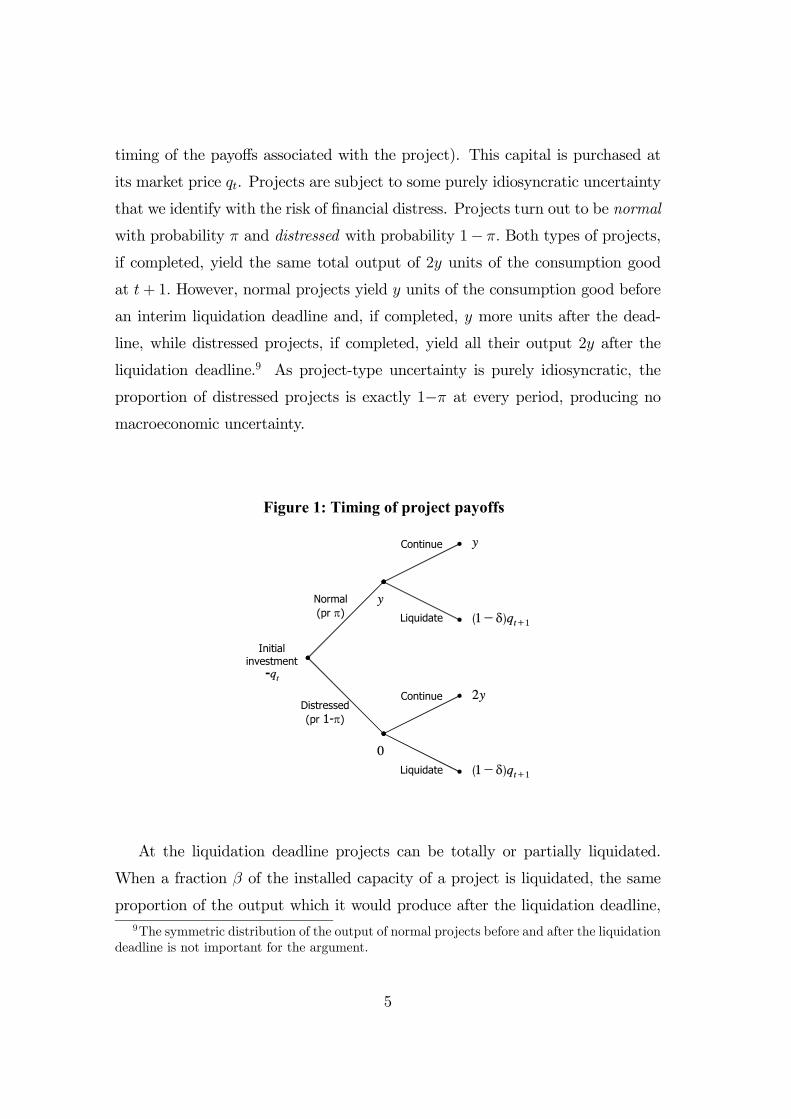
timing of the payoffs associated with the project). This capital is purchased at
its market price qt. Projects are subject to some purely idiosyncratic uncertainty
that we identify with the risk of financial distress. Projects turn out to be normal
with probability π and distressed with probability 1− π. Both types of projects,
if completed, yield the same total output of 2y units of the consumption good
at t+ 1. However, normal projects yield y units of the consumption good before
an interim liquidation deadline and, if completed, y more units after the dead-
line, while distressed projects, if completed, yield all their output 2y after the
liquidation deadline.9 As project-type uncertainty is purely idiosyncratic, the
proportion of distressed projects is exactly 1−π at every period, producing nomacroeconomic uncertainty.
Initial investment -qt
Normal (pr π)
Distressed (pr 1-π)
Continue
Liquidate (1-δ)qt+1
Continue
Liquidate (1-δ)qt+1
y
2y
y
0
Figure 1: Timing of project payoffs
At the liquidation deadline projects can be totally or partially liquidated.
When a fraction β of the installed capacity of a project is liquidated, the same
proportion of the output which it would produce after the liquidation deadline,9The symmetric distribution of the output of normal projects before and after the liquidation
deadline is not important for the argument.
5

if continued, is lost. However, for each initial unit of capital which is liquidated,
1−δ units can be sold to the entrepreneurs of the next cohort. So the liquidation
value of a period t start-up is (1 − δ)qt+1, which depends on both the physical
depreciation of capital before the liquidation deadline, δ, and the price of capital
at t+ 1.
Entrepreneurs are born penniless, so their projects have to be externally fi-
nanced. We assume that the relationship between financiers and entrepreneurs is
burdened by an agency problem: the output of a project is observable by both the
entrepreneur and her financiers, but it is not verifiable by the judge or court on
whom the enforcement of the contract depends (see [7]). Hence output-contingent
cash flow rights cannot be contracted upon.10 In contrast, the settlement of pay-
ments is verifiable so if a promised repayment is not settled, the relevant judge
or court can safely infer that the entrepreneur has defaulted. Also, as commonly
assumed in the literature, liquidation and the proceeds from the sale of liquidated
assets are verifiable. This allows an incomplete contract to be implemented that
fixes some repayment to be settled some time before the liquidation deadline and,
contingent upon the event of default, gives financiers the right to liquidate all or
a part of the project.
Such a contract leaves room for strategic default , that occurs when a non-
distressed entrepreneur defaults just in order to renegotiate some better terms.
The renegotiation will take place after it is already known whether the project’s
early output is y or 0, but before the liquidation deadline. We model the rene-
gotiation as a take-it-or-leave-it-offer game in which the financier makes the offer
with probability λ and the entrepreneur with probability 1−λ. Hence, the lower
is λ, the softer is the lending relationship for the entrepreneur.
It is quite common to view Chapter 11 of the US bankruptcy code as a court-
supervised renegotiation process.11 Such ‘supervision’ is rarely neutral: typically,10The “observable but not verifiable” assumption — like others in the model — is made for
analytical tractability rather than realism. Observability avoids the need to model bargainingunder asymmetric information; non-verifiability introduces an agency problem between debtorand creditor. This assumption could be partially relaxed (e.g. a certain part of the cash couldbe verifiable) without affecting the results.11See [1].
6

it tilts the terms of the contract in favor of one of the parties. The literature
considers Chapter 11 as tilted towards the entrepreneur, while the British law,
that insists on the strict enforcement of contracts, is put at the other end of the
bankruptcy-law spectrum.12
Formally, one can model the effects of moving from a tougher environment to
an American-type bankruptcy law as either a change in the bargaining power in
favor of the entrepreneur (i.e. a lower λ), or as a direct dilution of the liquidation
rights held by the secured lenders. We consider both formalizations.
In contrast with the consumption good in the above projects, capital can
be instantaneously produced and, thus, the industry that produces it bears no
agency problem. We assume that this industry is perfectly competitive and has
a technology described by a constant-returns-to-scale Cobb-Douglas production
function:
Nt = AXγt L
1−γt , (1)
where Nt is the period-t production of new capital, Xt and Lt are the inputs of
consumption good and labor, and γ ∈ [0, 1] is the elasticity to the consumptiongood input. For simplicity we assume that the supply of labor is inelastic and
equal to one. Moreover, we assume that
α ≡ 1γA−(1/γ) < y, (2)
which guarantees that the price of capital is low enough to make all projects to
be continued in the first-best economy (see Section 3).
Lastly, we assume that the economy starts functioning at t = 0 with an initial
condition given by some supply of old capital O0 > 0 coming from the liquidations
of the previous generation of entrepreneurs.12The British approach still leaves plenty of room for renegotiations, but they take place
out of court, and the law makes no attempt to affect the ‘natural’ outcome of the bargainingprocess; see [6].
7

3 Verifiable cash flows: the first best
To start with, it is useful to analyze, as a benchmark, an economy which is identi-
cal to the one just described except because entrepreneurs are not burdened with
an agency problem. We show that under our parametric assumptions projects are
never liquidated and the economy converges to a (unique) stationary equilibrium
after one period.
The supply of new capital can be derived by ordinary marginal-cost pricing
considerations. Remembering that the supply of labor is fixed and normalized to
one, the industry’s supply function becomes:
Nt =³qtα
´θ, (3)
where
θ ≡ γ
1− γ. (4)
The magnitude of α relative to y is fixed by assumption (2). The price-elasticity
is constant and equals θ, which rises from zero to infinity as γ moves from zero
to one.
We can now state the main result of this section.
Proposition 1 If project output is verifiable, the unique equilibrium features qt =
α for all t ≥ 1. No project is ever liquidated.
Proof. We start by establishing an upper bound to the market-price of capital:
since the demand of new capital never exceeds one, (3) implies qt ≤ α.
Next, we show that within this range of feasible prices, no project is ever liqui-
dated, and no project is ever left idle. Note that in the absence of cash-verifiability
problems the Modigliani-Miller theorem holds so all investment and liquidation
decisions are taken so as to maximize NPV. Consider first the liquidation decision
for the t-born cohort. By assumption (2), we have (1− δ)qt+1 < y, so a normal
project is never discontinued. As distressed projects have even greater continua-
tion value, 2y, their continuation is even more profitable. Thus no project is ever
8

liquidated in this economy, regardless of financial distress. Hence, when started
up, each project’s output has an expected present value of 2y. Since qt < 2y
investments have positive NPV and will be funded. It follows that from t = 1
onwards, the demand for new capital is exactly one, so its price is α, by (3).
Things are slightly different at t = 0, where some capital O0 is offered for sale
by the previous generation. In this case, the market clearing price of capital is
q0 = α (1−O0)1/θ < α.¥ (5)
4 Unverifiable cash flows: the contract
Our contract problem is similar to [4] and [8]: unverifiable cash flows can be
directly appropriated by the entrepreneur, who can only be induced to repay to
his financiers under a liquidation threat. The main difference is that the price
of capital has a critical effect on the problem. As we show in this section, the
start-up price qt affects the entrepreneur’s financial requirements and thus his
financiers’ participation constraint, while the liquidation price qt+1 affects his
incentives to default strategically.
When cash-flows are unverifiable, the first best is no longer attainable. If the
contract establishes that the project is never liquidated, as in the first-best case,
then, by the liquidation deadline and no matter the project has yielded some
output or not, the entrepreneur will claim that his project is distressed and he
has nothing with which to repay the financier at that stage. But obviously once
the project has yielded all its output the entrepreneur will simply ‘take the money
and run’. Although by the liquidation deadline the financier may know that the
entrepreneur is cheating (remember that output is observable), he cannot prove it
in court (since output is in that precise sense unverifiable). Evidently, if financiers
foresee this course of action, they will not fund to the entrepreneur in the first
place, despite all projects have positive NPV.
The standard incomplete-contract solution in this context is to provide the
financier with the right to liquidate all or a fraction of the project in case of
default. To illustrate how this will induce the entrepreneur to repay, suppose
9

that an entrepreneur born at t is obliged to repay a certain amount Rt < y in
period t + 1. Suppose that the project is not distressed but the entrepreneur
refuses to pay Rt. If the financier has to choose between fully liquidating the
project for (1 − δ)qt+1 and forgiving the entrepreneur, he will obviously choose
the first option.13 The entrepreneur would foresee the action and avoid (strategic)
default. A more refined version of this argument should take into consideration
the possibility of renegotiation between the entrepreneur and the financier. Figure
2 depicts the sequence of events, including the possibility of renegotiation, when
the project yields some early cash flow x before the liquidation deadline (in a
non-distressed project, we have x = y).
Project yields early
cash x
Repay R
Default
Leave it stand
Liquidation threat
Agree on R’<x
Liquidate
(2y-R, R) (requires x>R )
(2y, 0)
(2y-R’, R’)
(x, (1-δ)qt+1)
Figure 2: Events after early cash flow x realizes
If the financier has the chance to make the entrepreneur a take-it-or leave it
offer, he will be able to appropriate up to the project’s continuation value y. If
the entrepreneur has the chance to make the financier a take-it-or-leave-it offer he
would push his repayment down to the liquidation value of the capital, (1−δ)qt+1.13Remember that: (i) the financier cannot operate the project by himself, and that (ii) capital
will fully depreciate if the project is continued up to t+1. Hence, the best the financier can dois to liquidate the project and sell the remaining capital in the second-hand market at t+ 1.
10

Thus, the entrepreneur will choose not to default as long as the repayment Rt is
no larger than the expected renegotiated payment R0t = λy + (1− λ)(1− δ)qt+1.
Unfortunately, this solution involves a deadweight loss. When the project is
distressed (that is, if x = 0 in Figure 2), the entrepreneur faces a genuine cash
shortage and she has no choice but to default. In such a case, it is still in the
financier’s best interest to fully liquidate the project. Although the project still
has a continuation value that exceeds its liquidation value, the entrepreneur does
not have the liquidity to buy out the financier’s liquidation rights, nor can she
credibly commit to pay at t+ 1. In sum, if the lender is given the right to fully
liquidate the project, full liquidation will follow in case of distress.
However, the financier’s liquidation rights need not be so large. They should
be just sufficient to induce repayment when the project is not distressed. In
general, only a fraction βt of the capital will be pledged as collateral so that,
in case of default, lenders only have the right to liquidate such a fraction of
the project. In this case, the entrepreneur will choose not to default insofar as
Rt ≤ βt[λy + (1− λ)(1− δ)qt+1].
A contract is thus a pair (Rt,βt), where Rt is the debt-repayment, βt is the
collateral, and t is the date at which the contract is signed. The contract problem
for the entrepreneur born at t has the following form:
maxβt,Rt π(2y −Rt) + (1− π)(1− βt)2ys.t.:
(6)
πRt + (1− π)βt(1− δ)qt+1 = qt (participation constraint) (7)
Rt ≤ βt[λy + (1− λ)(1− δ)qt+1] (incentive constraint) (8)
π(2y −Rt) + (1− π)(1− βt)2y ≥ 0 (positive-profit constraint) (9)
Rt ∈ [0, y], βt ∈ [0, 1] (feasibility constraints) (10)
The participation constraint (7) holds with equality, reflecting that entrepreneurs
have all the bargaining power at the contracting stage.
When solving the program (6)-(10), we focus on βt; the repayment Rt can
always be obtained recursively, but its analysis is of limited interest for our ar-
gument. We analyze the problem with the aid of Figure 3, where the downward-
11

sloping PC line represents equation (7), and the shaded area above the upward-
sloping IC line represents the set of incentive-compatible contracts as defined in
equation (8). The two lines intersect at point
β (qt, qt+1) ≡ qt(1− δ) (1− λπ) qt+1 + λπy
. (11)
0
Figure 3: The contract problem
Rt
βtIC
1
PC
(1-λ)(1-δ)qt+1+ λy
optimal contract
feasible set
Proposition 2 The optimal contract is βt = β (qt, qt+1), provided that β (qt, qt+1) ≤1. When β (qt, qt+1) > 1, the entrepreneur is credit-rationed and the project re-
ceives no funding.
Proof. We start by showing that the problem’s constraints can be reduced to
equations (7), (8), and βt ≤ 1 only. First notice that under (10), constraint (9)is redundant, while Rt ≤ 0 and βt ≤ 0 are clearly incompatible with (7) and
(8). Second, substituting βt = 1 into equation (7) we get Rt = λ (1− δ) qt+1 +
(1− λ) y, as represented in Figure 3; but then it follows that the constraint
Rt ≤ y will never be binding since qt+1 ≤ α < y by assumption (2) (recall from
Proposition 1 that qt+1 would reach its maximum value of α if no project started
up at t were liquidated).
12

Hence, the feasible set for the program (6)-(10) is determined by (7), (8) and
the feasibility constraint βt ≤ 1. Graphically, the feasible set is the section of thePC line that belongs to the IC set (shaded) and is below the βt = 1 line: the
bold segment in Figure 3. Clearly, if the IC and the PC lines intersect at a point
with βt > 1, then the feasible set is empty and the project is credit-rationed.
Substituting equation (7) into (6), the objective function (6) can be written
as
v(qt, qt+1) = 2y − qt − (1− π)βt [2y − (1− δ) qt+1] . (12)
It follows that the objective function is maximized when βt is minimized. Hence,
the optimal contract is the point with the lowest βt within the feasible set.
Namely, β (qt, qt+1), provided that β (qt, qt+1) ≤ 1.¥
The economic intuition behind Proposition 2 is best described through equa-
tion (12). It decomposes the entrepreneur’s profit into the first-best output of the
project, minus the purchase-price of the unit of capital invested in it, minus the
expected deadweight loss that results from the agency problem. The latter term
equals the probability of default, times the fraction of the project that the lender
can liquidate in case of default βt, times the difference between the continuation
and liquidation values of the project. The optimal contract should minimize the
expected deadweight loss, and that is done by minimizing the size of the collat-
eral. Clearly, the smaller is the collateral, the smaller is the scope for losses due
to premature liquidation.
Proposition 1 provides one of the model’s basic building blocks, establishes a
relationship between market prices and agency problems. Note that
∂β
∂qt> 0 and
∂β
∂qt+1< 0. (13)
Namely, when the current price of capital increases, entrepreneurs’ funding re-
quirements increase and debt repayments must increase as well. Each entrepre-
neur will have to provide more collateral in order to ensure his financiers that he
has no incentive to engage in strategic default. In contrast, when the next-period
13

price of capital increases, strategic default becomes less attractive, permitting
repayments to be enforced with less collateral. In short, the underlying incen-
tive problem is more severe when the purchase price of capital is high and its
liquidation price is low.
Lastly, notice that the contract that we have just characterized shares many
features with real-world debt contracts; particularly, the repayment Rt is not
conditional on the project’s output and is enforced through a liquidation threat
whose effectiveness is tied to the value of the collateralized assets. We shall
henceforth refer to the financier as a lender, and to the entrepreneur as a borrower.
More importantly, identifying the financial arrangement as ‘debt’ enables us to
interpret what happens after default as ‘bankruptcy’ and to analyze the effects
of bankruptcy law.
5 Competitive non-rationing equilibria
We construct a competitive equilibrium by combining the supply schedule (3)
with the solution of the contract problem derived in Section 4. We limit our-
selves to non-rationing equilibria. Tractability is the only reason: non-rationing
equilibria are governed by a first-order non-linear difference equation (equation
(22) below) which is complicated enough. Because every entrepreneur is funded
in such an equilibrium and the size of both the population of entrepreneurs and
their projects are fixed, investment per cohort is constant over time (and equal
to one). In contrast, once the entrepreneurs are credit-rationed (at some date),
investment is no longer constant and prices follow a second-order non-linear dif-
ference equation, which is much more difficult to analyze.
To facilitate the presentation, let:
a ≡ (1− δ) (1− λπ) , b ≡ λπy, c ≡ (1− δ) (1− π) , (14)
so that
β (qt, qt+1) ≡ qtaqt+1 + b
. (15)
Formally, the equilibria on which we focus are defined as follows:
14

Definition 1 A competitive, rational-expectations, non-rationing equilibrium is
a sequence {qt}∞t=0 that satisfies³qt+1α
´θ= 1− cβt, (16)
βt = β (qt, qt+1) , (17)
β (qt, qt+1) ≤ 1, (18)
and the initial condition (5).
Note the important differences between this economy and the benchmark
economy described in Section 3. With verifiable cash flows, no project is ever
liquidated, the production of capital equals one in every period, and the price of
capital is constant and equal to α. With unverifiable cash flows, a fraction βt of
the capital invested in each project at date t is pledged as collateral, of which
a fraction c becomes reusable, through liquidation and sale in the second-hand
market, at t+1. As reflected in the market clearing condition (16), the production
of new capital will typically be lower than one and its price will typically be lower
than α.
Our endogenous-cycles results depend crucially on the non-linear nature of
price dynamics. This non-linearity complicates the analysis of existence. Solving
for βt in (16) and substituting the resulting expression into equation (17) gives
the temporal equilibrium condition
g (qt+1) = β (qt, qt+1) , (19)
where
g (qt+1) ≡ 1c
·1−
³qt+1α
´θ¸. (20)
Equation (19) allows us to explicitly solve for qt, giving rise to a well-defined
backward looking difference equation
qt = φ (qt+1) . (21)
15

However, since our dynamic system is forward looking (i.e. with an initial condi-
tion given by (5)), we are interested in the difference equation
qt+1 = f(qt) ≡ φ−1 (qt) , (22)
which will be well-defined if any price qt prevailing at some period t can be
associated with a unique price qt+1 at t + 1 (in other words, if φ is monotonic
and, hence, invertible over the relevant range). Additionally, for a sequence of
prices produced by such difference equation to correspond to a non-rationing
equilibrium, we should make sure that all pairs (qt, qt+1) in the sequence satisfy
the non-rationing constraint (18). The following lemma shows that, if we assume
α ≤ b, (23)
then the difference equation is well-defined, the non-rationing constraint is satis-
fied, and there exists a unique stationary non-rationing price q∗.
Lemma 1 Under assumption (23), there exists a well-defined sequence of com-
petitive, rational-expectations, non-rationing equilibrium prices, and a unique sta-
tionary price q∗.
Proof. See the Appendix.
In Figure 4 we plot the values of g (qt+1) and β (qt, qt+1) against the values of
qt+1, for a given value of qt. The graphs of both functions are downward sloping.
The graph of g crosses the vertical axis at 1/c and the horizontal axis at α,
and it is concave for θ > 1 and convex for θ < 1. The graph of β crosses the
vertical axis at qt/b and falls asymptotically towards the horizontal axis; it is
always convex and shifts upwards when qt increases. Assumption (23) guarantees
that the intercept of g is above the intercept of β for all qt ≤ α, which in turn
guarantees that, for any given qt, the graphs of g and β intersect at least once at
some qt+1 < α. Actually, for θ > 1, the concavity of g directly implies that this
intersection is unique and defines the value of f(qt). For θ < 1, the problem might
in principle be more complicated but, as shown in the lemma, it happens that
16

(23) is also sufficient for uniqueness. Importantly, the fact that the intercept of β
is below the intercept of g implies that the graph of β crosses the graph of g from
below, so when qt increases, β shifts upwards, and the intersection occurs at a
lower qt+1. In other words, the difference equation has negative slope (f 0(qt) < 0).
0
Figure 4: Analysis of the f function
qt+1
βt
α
c1
g, θ>1
g, θ<1 β
bα
qt↑
Figure 5 depicts the graph of the difference equation (22). The stationary price
q∗ corresponds to its intersection with the 45◦ line. It is well-known that with a
non-linear monotonically decreasing difference equation like ours, the equilibrium
will consist on a sequence of prices that cyclically converge to either the stationary
price q∗ (stable equilibrium) or a limit cycle with a periodicity of two (periodic
equilibrium). To analyze the latter, we define
f2 (q) ≡ f [f (q)] . (24)
17

0
Figure 5: Limit cycles
qt
qt+1
45o
α
f
f2
bust start-up
boom start-up
qL qH
q*
Hence,
Proposition 3 If f 0 (q) > −1, the equilibrium converges to the stationary point.If f 0 (q) < −1, the equilibrium converges to a two-period stable limit cycle.14
Proof. See the Appendix.
Since we will focus on limit cycles, their mechanics is worth some further
elaboration.15 If a limit cycle exists, then long-run equilibrium prices would
fluctuate from qL to qH and vice versa. A low spot price, qL, indicates that the
demand for new capital is at a relatively low level. That is due to a relatively large
amount of capital coming from liquidations and offered for sale in the second-
hand market. In such a period, the production of the consumption good is also
relatively low due to so much premature liquidation. It seems reasonable to dub14This proposition does not show that the limit cycle is unique. However, simulating the
model, we never found more than one limit cycle. In case of several limit cycles, the resultsabove apply to the one next to the stationary point.15We focus on limit cycles just because this is where the results are most dramatic, as all
effects survive for the long run. A weaker version of the results can be derived by examiningthe dynamics of the system around its (stable) stationary point.
18

such a period a ‘bust’. For similar reasons, we dub a period with high capital
prices a ‘boom’.
Since each entrepreneur operates for two periods, each goes through both a
boom and a bust. However, entrepreneurs differ greatly according to the period
at which they start up. Someone starting up in a boom would operate under
tighter financial conditions, relative to a bust start-up: she has to borrow a
larger amount in order to finance the purchase of expensive capital, and has to
repay the debt when capital prices are depressed. Even if she is not distressed,
she has a stronger incentive to default strategically; if distressed, her capital will
be liquidated at a lower price (see Figure 5). Hence, to get funding, she will have
to mortgage a larger fraction of her project (see the partial derivatives in (13)).
Hence, the mechanics of our equilibrium cycle: suppose that period t is a
boom. Then period-t start-ups would be forced to pledge a large amount of
collateral against the funds they borrow. As lenders foreclose all the collateral
of distressed entrepreneurs, the supply of second-hand capital at t + 1 would
increase, depressing its price and pushing the economy into the bust. However,
the low price of capital would ease financial conditions for t+ 1 start-ups, which
would be able to borrow against less collateral. But then, the supply of second-
hand capital at t+ 2 would be relatively small, which would push capital prices
and production back into a boom. And so on.
More insight into the mechanics of the cycle can be obtained with the aid
of Figure 6, a bifurcation diagram. The model is simulated with the following
parameters: π = 0.6, λ = 0.5, δ = 0.10, α = 5 and y = 17.5. One may verify
that assumption (23) is satisfied. The stationary price q∗ and the two periodic
prices, qL and qH are plotted (when they exist) against various levels of θ. As
one should anticipate from Figure 4, the stationary point increases with θ, as the
g function moves outwards. Also consistent with Figure 4 is that as θ increases,
the slope of the g curve increases and shifts in the β curve (due to changes in qt)
tend to have smaller effects on qt+1. The f function becomes flatter, excluding
periodic equilibria for high θs. Intuitively, when the price-elasticity of the supply
of new capital increases, the price of capital becomes less sensitive to changes in
19

the supply of second-hand capital so cyclicality is less pronounced. For low θs,
large price changes generate great variability in financial constraints along the
cycle, and feed back into the cycle itself.
Figure 6: Bifurcation diagramπ=0.6, λ=0.5, δ=0.1, α =5, y=17.5
θ
q
q*
qL
qH
It is noteworthy that our model seems to capture the essence of the notion
of ‘financial instability’. Consider an economy with a stable limit cycle, and an
initial condition that is just off the stationary point q∗. Since the stationary point
is not stable (see Proposition 3), the economy will start oscillating away from q∗.
Initially, the amplitude of these oscillations is very small; we can make them as
small as we wish by bringing the initial point closer to q∗. But gradually, the
cycle will build up until it converges to the limit cycle. This build-up of ‘insta-
bility’ is wholly endogenous, and will take place without the economy absorbing
any exogenous shock. Rather, market prices coordinate lenders and borrowers
into collateral positions that amplify the cycle. Moreover, the whole equilibrium
is driven by financial factors: we know, from Proposition 1 that without finan-
cial frictions in the form of non-verifiable cash-flows, the system would converge
up-front to an equilibrium with stable prices and output (and with higher net
20

income).
6 Bankruptcy-law reform
Since the fluctuations in our model are driven by the endogenous dynamics of
collateralized borrowing and asset liquidation, it is interesting to examine how
court involvement in the resolution of financial distress would affect the business
cycle. As noted above, authors such as [12] have argued that once bankruptcy
law is analyzed within a proper general-equilibrium framework, the rationale for
Chapter 11 becomes evident. Our model seems to provide prima facie support to
such a claim: since liquidations are driven by financial distress rather than neg-
ative continuation values, and since distressed asset-sales have an adverse price
effect, which by itself tightens the financial constraints of other business (of the
same cohort), a softer bankruptcy law might help to stabilize the economy. How-
ever, the analysis below demonstrates the fallacy of this argument in a dynamic
equilibrium framework.
Our model offers two ways through which court involvement can soften bank-
ruptcy law. Firstly, the court can dilute the liquidation rights of the secured
lenders, disallowing them to exercise their rights on a certain part of the collat-
eral. Thus, the effective collateral, β, decreases below the nominal collateral, βN .
Secondly, the court can establish bargaining procedures that favor the borrower.
In the context of our model, decrease λ. We analyze both formalizations.
In line with the observations of [3], we assume that the reform is announced
when the economy is already in a bust. We also assume that the reform is not
anticipated in advance, so that the current debt contracts were signed under the
expectation that the contract would be implemented under the old law. Clearly,
in a situation like that contracts might be renegotiated, which previously hap-
pened only off the equilibrium path. One might think that in such a case it
matters whether the parties renegotiate before or after the uncertainty about fi-
nancial distress is resolved. As a matter of fact, in our case it makes no difference
and we thus assume, without loss of generality, that renegotiations take place
21

ex-post, after the uncertainty is resolved.
6.1 A dilution of liquidation rights
Let βN be the lender’s ‘nominal’ liquidation rights as written in the debt contract,
and assume that the bankruptcy court cancels a fraction ξ while enforcing the
contract, so that the ‘effective’ liquidation rights are
β = (1− ξ)βN . (25)
Proposition 4 A small dilution factor ξ has no long-run effect. Introducing it
in the bust produces a transitory stabilizing effect.
Proof. To see why the long-run equilibrium is unaltered, note that if the nominal
collateral is βN = β/ (1− ξ), then after dilution the effective collateral remains
the same, and the program (6)-(10), remains the same in terms of effective col-
lateral. Hence, the equilibrium conditions in Definition 1 remain unaltered, and
so is the long-run equilibrium. The argument holds for small ξs only because the
inflation of nominal collateral may lead to the violation of the feasibility condition
βN ≤ 1.In the short run, however, before contract terms are fully adjusted, the dilution
decreases the effective collateral supporting the existing credit relationships: the
incentive constraint (8) no longer holds so that the repayment R will have to
be renegotiated downwards.16 The smaller amount of liquidation will have a
positive, short-run effect on prices, capital production, and output. Clearly, if
the reform takes place in the bust, the effect is stabilizing.¥
In terms of Figure 3, the dilution would move the effective β downwards,
away from the optimal-contract point. Being below the IC line, the parties will
have to adjust the repayment R, moving horizontally. Note that the renegotiated
contract will be below the original participation constraint, which implies that the16Recall that in the absence of unexpected events such as a reform in bankruptcy law, contract
renegotiations are an off-the-equilibrium-path phenomenon.
22
law-reform generates a one-off wealth transfer from lenders to borrowers, which
explains the short-run stabilizing effect of the policy. In the long run, both the
IC and the PC curves are not affected.
6.2 Giving the borrower more bargaining power
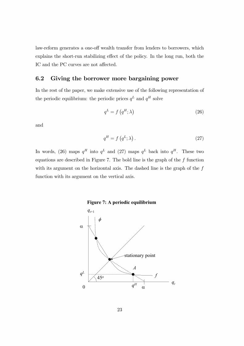
In the rest of the paper, we make extensive use of the following representation of
the periodic equilibrium: the periodic prices qL and qH solve
qL = f¡qH ;λ
¢(26)
and
qH = f¡qL;λ
¢. (27)
In words, (26) maps qH into qL and (27) maps qL back into qH . These two
equations are described in Figure 7. The bold line is the graph of the f function
with its argument on the horizontal axis. The dashed line is the graph of the f
function with its argument on the vertical axis.
0
Figure 6: A periodic equilibrium
qtα
α
qt+1
45o
qH
qLf
φ
A
stationary point
Figure 7: A periodic equilibrium
23

We can now analyze the effect of a reform that softens bankruptcy law by
giving more bargaining power to the borrower:
Proposition 5 For a ‘moderately-cyclical’ economy, a reform that gives the bor-
rower more bargaining power will increase the long-run amplitude of the business
cycle; this reform will have no short-run effects.
Proof. See the Appendix.
Intuitively, when λ decreases the IC line of Figure 3 would rotate counter-
clockwise. Again, repayments will be renegotiated, moving the contracts hori-
zontally and towards the left, at exactly the same β, so that the one-off wealth
transfer from lenders to borrowers will have no short-run effect on the amount of
liquidation. In the long run (for given market prices), the feasible set will shrink.
The borrower will have to pledge a greater fraction of her capital as collateral in
order to commit herself not to default strategically, now that she has more bar-
gaining power. With more collateral there will be more liquidations, a stronger
effect of financial distress on the price of capital and a greater cyclicality of the
economy.
If a real-world softening of bankruptcy law (such as, say, the introduction of
Chapter 11 in the US) is a mixture of the two formalizations that we have just
explored, then introducing it in the bust will have a short-run stabilizing effect,
but it will increase cyclicality in the long run.17 So it seems that such a policy
is a dubious stabilizing policy, specially once its short-run benefits pass and its
dynamic general equilibrium implications come into effect.17This result leaves two possible (not necessarily mutually exclusive) interpretations for the
observation that US bankruptcy law was softened during busts ([3]). The first is a political-economy one: a Chapter-11 type of law reform is a policy introduced by a myopic governmentthat simply ignores the long-run effects. The second interpretation is a more of a historical-institutional one: initially, bankruptcy legislation was an ad-hoc debt relief policy, employedby a government that still lacked more refined instruments such as monetary and fiscal policy.The application of the law created legal precedents and ended up being implemented both inbooms and in busts, exacerbating the economy’s cyclicality.
24

7 Other stabilizing policies
The absence of stabilizing long-run effects in bankruptcy law reform is due to the
adjustment of contract terms that follows the rational anticipation of the way
the contract will be enforced under the new law. However, rational expectations
and subsequent adjustments in the equilibrium do not invalidate all possible
stabilizing policies. In particular, in this section we show that bail-outs and an
active management of interest rates along the cycle (monetary policy?) can have
long-run stabilizing effects. The key difference is that these policies involve a
sustained transfer of wealth from less to more financially-constrained agents.18
7.1 Bail outs
Suppose that the government initiates a policy of recompensing the debt of
(some) borrowers in the bust (remember that bust borrowers are those that hav-
ing started up during the boom, when the price of capital is high, carry over a
larger amount of collateralized debt). Suppose that the subsidy is funded by a
lump-sum tax on the businesses that mature during the boom (i.e. those started
up during the bust, when the price of capital is low). Of course, the govern-
ment operates under the same informational constraints as the private sector:
cash-flows are non-verifiable. Thus the government cannot run a bail-out policy
exclusively for the firms that declare default since in such case all firms would
declare default. So we assume that the government recompenses the debt of a
fraction ψ of all companies, chosen at random. In contrast, the tax can only be
levied on the firms serving their debt, whose incentive constraint will be tightened
by this additional repayment requirement.
From the description above it should be clear that the tax, T , inserts a wedge
between what a borrower pays, say R0 = R + T, and what its lender gets, R.
SubstitutingR0 forR in the incentive constraint (8), working through the contract
problem again, substituting the result in the equilibrium condition, and focusing18Our model has no money and thus no monetary policy. Still, it is reasonable to expect
that real-world monetary policy might achieve the effect on real interest rate charges that our‘active interest-rate policy’ requires.
25

on a periodic equilibrium, we getµqH
α
¶θ
= 1− cqL + πT
aqH + b. (28)
Note that, for given prices of capital, the tax tightens the incentive constraint
and thus forces an increase in the collateral taken up by the lender.
For the subsidized cohort of entrepreneurs, the bail-out policy decreases the
probability of default from (1− π) to (1− π) (1− ψ). Substituting the new prob-
abilities of success and failure into the participation constraint (7) and taking the
same steps as with equation (28) we getµqL
α
¶θ
= 1− (1− ψ) cqH
aqL + b+ λψ (1− π) [y − (1− δ) qL]. (29)
Bail-outs relax the participation constraint of the entrepreneurs who start pro-
ducing in the bust and thus (for given prices of capital) allow for a reduction
in the amounts of collateral that they offer. Additionally, as less projects are
liquidated (notice that parameter c is factored by 1− ψ), even less capital good
gets finally liquidated.
To close the system, we assume that the government balances its budget in
every period so
ψRL = πT , (30)
where
RL =qH£λy + (1− λ) (1− δ) qL
¤aqL + b+ λψ (1− π) [y − (1− δ) qL]
(31)
is the debt-repayment of bust entrepreneurs.
Proposition 6 A small-scale bail-out policy would decrease the long-run ampli-
tude of the business-cycle.
Proof. See the Appendix.
26

7.2 Active interest-rate policy
The structure of an active interest-rate policy is even simpler: bust repayments
are subsidized, while boom repayments are taxed. Namely, prices are determined
by the system
qH = fH¡qL;T
¢, (32)
qL = fL¡qH ; s
¢, (33)
where T and s must satisfy the government’s budget constraint
π (T − s) = 0. (34)
The functions fH and fL are implicitly defined by equations with the same form
as (28) (where, in the case of fL, −s replaces T ).
Proposition 7 A small-scale active interest-rate policy would decrease the am-
plitude of the business-cycle in the long run.
Proof. See the Appendix.
Why are the results in this section so different than those of the previous
section? The reason is that the fluctuations in this economy are driven by finan-
cial constraints. Financial constraints can be relaxed through wealth transfers
from the less constrained to the more constrained agents —in our case, from the
entrepreneurs who start producing in the boom to those who start producing in
the bust. As we have seen, bankruptcy-law reform does not generate such an
effect. If anything, it makes the incentive constraint more binding and, thus, ex-
acerbates the problems associated with financial constraints. More “traditional”
measures such as interest-rate or bail-out policies perform the stabilizing role
more effectively.
27

8 Welfare analysis
What are the welfare properties of the type of stabilizing policies described above?
In answering this question, we must draw a clear line between those welfare-
improving mechanisms that could be directly implemented by private agents and
those that can only be implemented by the government. This distinction is more
difficult to make within incomplete-contracts models, since some of the policies
may consist in widening an implicitly restricted set of contracting possibilities.
Indeed, the contract we have considered leaves room for a type of improve-
ment that government subsidies and taxes might achieve but, in principle, private
agents might also achieve by themselves. Specifically, consider a subsidy to the
initial investment sI , so that the debt contract becomes β¡qt − sI , qt+1
¢; since
investment always equals one, this subsidy requires a government budget B = sI .
For given market prices and a ‘small’ subsidy, the marginal effect on β of this
kind of government expense is
dβ
dB= − 1
aqt+1 + b. (35)
Now, consider an alternative subsidy sL to liquidation prices under which the
debt contract features β¡qt, qt+1 + s
L¢and the required government budget is
B = cβ¡qt, qt+1 + s
L¢sL. Then
dβ
dB= −a
c
1
aqt+1 + b. (36)
Since a > c, it follows that a balanced-budget policy combining a tax on the initial
investment of a given generation of entrepreneurs with a subsidy that supports the
liquidation prices of their projects could reduce the dead-weight losses associated
with their debt contracts. Notice, however, that this policy could be replicated
by the private agents without the need of government intervention. In essence,
entrepreneurs could borrow in excess of the initial cost of investment, keep the
difference in a safe account and commit it to indemnifying lenders against credit
losses. Without contradicting our initial constraints on contract design, estab-
lishing a cash payment contingent on the verifiable event of liquidation should be
28

feasible. This self-provided insurance scheme has pure strategic value: facing a
higher liquidation value, the lender would be a tougher bargainer vis-a-vis bor-
rowers who defaulted strategically, but then the amount of collateralized assets
necessary to prevent strategic default would diminish and, thus, the amount of
capital liquidated in the case of genuine distress.
Interestingly, the above opportunity to improve on the original debt contract
vanishes when the lender already has all the bargaining power, λ = 1, since then
a = c. It is easy to check that with λ = 1 interest-payment subsidies such as those
analyzed in a previous section are as effective (per unit of government expense)
as the two subsidies considered above. Hence we will simplify the discussion on
tax/subsidy schemes by focusing on the case with λ = 1. On the other hand, bail-
outs are in general less effective than more targeted tax/subsidy schemes as they
allocate a significant part of the budget to firms which are not cash-constrained,
so we shall not consider them any further. Finally, softer bankruptcy laws will
not be considered either as we have shown that their stabilizing effect is, at best,
limited to the short-run.
We thus focus on tax/subsidy schemes based on the subsidization of the
initial investment of some entrepreneurs and ask whether they bring about a
Pareto-improvement in the laissez-faire equilibrium (16)-(18). The definition
of constrained Pareto optimality that we use deserves some comments. First,
we consider the welfare of both entrepreneurs and the workers employed in the
capital-good industry. As lenders always receive the (zero) market rate of return,
they can be safely ignored. Second, we assume that lump-sum taxes can be im-
posed on workers, but not on entrepreneurs. The reason is that the government
faces the same enforcement problem as the lenders, so it could only extract cash
from the entrepreneurs that revealed themselves as not being distressed, that is,
by imposing a tax on debt repayments. But taxing debt repayments will undo
the effect of the subsidy to the initial investment.
A first question to analyze is whether a subsidy to the initial investment s,
financed by lump-sum taxes on the workers T , may increase the price of the
capital good and, hence, wages w sufficiently so as to compensate the workers for
29

the tax imposed on them. That would require a strong ‘multiplier effect’: start-
up subsidies would decrease collateral requirements and thus liquidations, this
would increase the demand for new capital and thus the price of capital. This,
in turn, will improve enforceability (see equation (13)), decrease liquidation even
further, and cause a further increase in the price of capital. Although financial
imperfections might, in principle, allow for such a multiplier effect to be welfare
increasing, this is not the case.
Consider first a stable steady state equilibrium with
q = f (q − s) , w = (1− γ) q³ qα
´θ− T , T = s. (37)
It tuns out that
∂w
∂q=³ qα
´θ< 1, (38)
so a necessary condition for the existence of a Pareto improvement is dqds> 1.
However,
1 >dq
ds|s=0= − f 0 (q)
1− f 0 (q) > 0 (39)
since stability requires −1 < f 0(q) < 0.A similar, albeit more cumbersome, reasoning applies to a periodic equilib-
rium. In this case it is convenient to describe the tax-subsidy scheme as consisting
of a subsidy τs for the boom cohort and a subsidy (1− τ) s for the bust cohort,
with τ ∈ [0, 1], so that
qL = f(qH − τs), qH = f(qL − (1− τ) s). (40)
A Pareto improvement would require that both boom and bust start-ups are
better off
dv(qH − τs, qL)
ds> 0,
dv(qL − (1− τ) s, qH)
ds> 0, (41)
where v is defined in (12), and that both boom and bust workers are also better
30

off19 µqH
α
¶θdqH
ds+
µqL
α
¶θdqL
ds> 1. (42)
We can now prove:
Proposition 8 With λ = 1, any long-term equilibrium, periodic or stationary,
is constrained Pareto efficient.
Proof. See the Appendix.
Thus, in what sense might a stabilizing policy be socially desirable? Apart
from additional non-modeled considerations (such as imperfect consumer-debt
markets that do not allow long-lived workers to smooth consumption over the
cycle), one might think that a stabilizing policy that spreads financial constraints
more evenly over the boom and the bust might decrease their overall ‘average’
effect upon the economy. We prove that this is actually the case, at least for
the case where f is concave, which is usually the case for periodic equilibria (see
Figure 6).
Proposition 9 Suppose that f is concave. With λ = 1, a stabilizing interest-
rate policy (namely a subsidy to more-constrained start-ups financed by a tax on
less-constrained start-ups) will increase the through-the-cycle value of the entre-
preneurial sector. Such a policy, however, may make workers worse off.
Proof. See the Appendix.
9 Conclusions
In this paper we provide an analysis of the interrelations between cyclical move-
ments in financial distress and various policy measures intended to mitigate the
consequences of financial distress, including bankruptcy law. The analysis is de-
veloped in the context of a dynamic model of entrepreneurial financing where19As workers can be lump-sum taxed, we can abstract from the exact allocation of taxes and
welfare across boom and bust participants.
31

asset liquidations are a second-best implication of the existence of a contract
enforcement problem. We show the contribution of this problem to the emer-
gence of cyclical movements in the economy. Our main finding is that softening
bankruptcy law produces no reduction in cyclicality, while other, more traditional
measures such as like bail-outs, active interest-rate policies or various subsidies to
financially constrained firms may have stabilizing effects and increase aggregate
net income.
The model is deliberately simple since the joint analysis of financial distress,
bankruptcy law, and macroeconomic stability in a dynamic general-equilibrium
setup can easily become mathematically intractable. Future research could re-
lax some of our assumptions in order to gain realism. For example, one could
consider more realistic distributions of project cash flows, allow for a verifiable
component in them, and add states of nature where projects have a negative
continuation value so that liquidation is socially efficient. Another challenge is to
model projects that last more than two periods; in that case, the relevant invest-
ment and liquidation decisions might depend on the entire path of future prices,
leading to more complex (and possibly more realistic) dynamics of liquidation
and prices. Such a model should surely be analyzed numerically.
32
Appendix
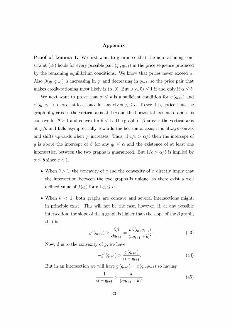
Proof of Lemma 1. We first want to guarantee that the non-rationing con-
straint (18) holds for every possible pair (qt, qt+1) in the price sequence produced
by the remaining equilibrium conditions. We know that prices never exceed α.
Also β(qt, qt+1) is increasing in qt and decreasing in qt+1, so the price pair that
makes credit-rationing most likely is (α, 0). But β(α, 0) ≤ 1 if and only if α ≤ b.We next want to prove that α ≤ b is a sufficient condition for g (qt+1) and
β (qt, qt+1) to cross at least once for any given qt ≤ α. To see this, notice that, the
graph of g crosses the vertical axis at 1/c and the horizontal axis at α, and it is
concave for θ > 1 and convex for θ < 1. The graph of β crosses the vertical axis
at qt/b and falls asymptotically towards the horizontal axis; it is always convex
and shifts upwards when qt increases. Thus, if 1/c > α/b then the intercept of
g is above the intercept of β for any qt ≤ α and the existence of at least one
intersection between the two graphs is guaranteed. But 1/c > α/b is implied by
α ≤ b since c < 1.
• When θ > 1, the concavity of g and the convexity of β directly imply that
the intersection between the two graphs is unique, so there exist a well
defined value of f(qt) for all qt ≤ α.
• When θ < 1, both graphs are concave and several intersections might,
in principle exist. This will not be the case, however, if, at any possible
intersection, the slope of the g graph is higher than the slope of the β graph,
that is,
−g0 (qt+1) > ∂β
∂qt+1=aβ(qt, qt+1)
(aqt+1 + b)2 . (43)
Now, due to the convexity of g, we have
−g0 (qt+1) > g (qt+1)
α− qt+1 . (44)
But in an intersection we will have g (qt+1) = β(qt, qt+1) so having
1
α− qt+1 >a
(aqt+1 + b)2 (45)
33
is a sufficient condition for uniqueness. It turns out that the above inequal-
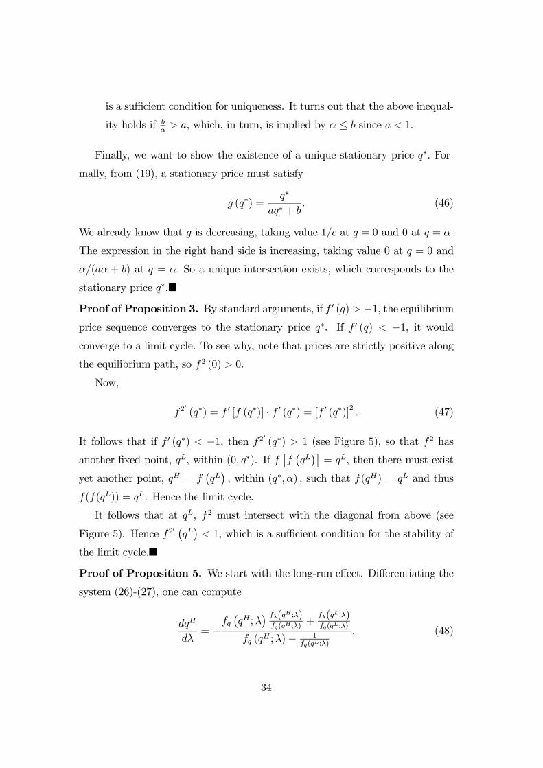
ity holds if bα> a, which, in turn, is implied by α ≤ b since a < 1.
Finally, we want to show the existence of a unique stationary price q∗. For-
mally, from (19), a stationary price must satisfy
g (q∗) =q∗
aq∗ + b. (46)
We already know that g is decreasing, taking value 1/c at q = 0 and 0 at q = α.
The expression in the right hand side is increasing, taking value 0 at q = 0 and
α/(aα + b) at q = α. So a unique intersection exists, which corresponds to the
stationary price q∗.¥
Proof of Proposition 3. By standard arguments, if f 0 (q) > −1, the equilibriumprice sequence converges to the stationary price q∗. If f 0 (q) < −1, it wouldconverge to a limit cycle. To see why, note that prices are strictly positive along
the equilibrium path, so f2 (0) > 0.
Now,
f20(q∗) = f 0 [f (q∗)] · f 0 (q∗) = [f 0 (q∗)]2 . (47)
It follows that if f 0 (q∗) < −1, then f20 (q∗) > 1 (see Figure 5), so that f2 has
another fixed point, qL, within (0, q∗). If f£f¡qL¢¤= qL, then there must exist
yet another point, qH = f¡qL¢, within (q∗,α) , such that f(qH) = qL and thus
f(f(qL)) = qL. Hence the limit cycle.
It follows that at qL, f2 must intersect with the diagonal from above (see
Figure 5). Hence f20 ¡qL¢< 1, which is a sufficient condition for the stability of
the limit cycle.¥
Proof of Proposition 5. We start with the long-run effect. Differentiating the
system (26)-(27), one can compute
dqH
dλ= −
fq¡qH ;λ
¢ fλ(qH ;λ)fq(qH ;λ)
+fλ(qL;λ)fq(qL;λ)
fq (qH ;λ)− 1fq(qL;λ)
. (48)
34

Note that we have
dqi
dλ|f(qi;λ)=const= −fλ (q
i;λ)
fq (qi;λ), (49)
for i = L,H, so (48) can be written as
dqH
dλ=fq¡qH ;λ
¢ · dqHdλ|f(qH ;λ)=const +dqL
dλ|f(qL;λ)=const
fq (qH ;λ)− 1fq(qL;λ)
. (50)
Equation (50) has the following graphical interpretation: the denominator is the
difference between the slopes of the f and the φ functions at point A of Figure
7, the numerator is the sum of the vertical shifts in f and φ due to the change
in λ. The denominator of (50) must be positive: by Proposition 3, f is steeper
than φ at the stationary point, so at point A, φ is steeper than f –recall that
both derivatives are negative.
Also one can clearly see that
dqH
dλ|f(qH ;λ)=const= πqH
y − (1− δ) qL
aqL + b> πqL
y − (1− δ) qH
aqH + b=dqL
dλ|f(qL;λ)=const
(51)
but, in a moderately cyclical economy qH will be close to the stationary point,
implying that fq¡qH ;λ
¢< −1, so the numerator of equation (50) is negative and
thus, dqH
dλ< 0.
By a parallel reasoning, it also follows that dqL
dλ> 0. Namely, the amplitude of
the cycle falls when λ increases. Remember that λ measures the lender’s power.
Hence, a softer system (lower λ) would increase the amplitude of the business
cycle.
As for the short-run, note that after an unanticipated fall in λ the incentive
constraint (8) no longer holds and repayments, R, will be renegotiated downwards
following strategic default. However collateral and, thus, liquidations in case of
financial distress will not vary.¥
Proof of Proposition 6. The logic of the proof is the same as in Proposition
5. Let the functions fH and fL be implicitly defined by (28) and (29) so as to
describe situations with bail-outs and taxes, respectively:
qH = fH¡qL;T
¢and qL = fL
¡qH ,ψ
¢. (52)
35

Note that with ψ = 0, we would have fH = fL = f. We consider a small-scale
bail-out policy as a perturbation of Figure 5, which depicts the ψ = 0 case.
Similar to the differential (50) we now have
dqH
dψ=fLq¡qH ;ψ
¢ · dqHdψ|fL(qH ;ψ)=const +dqL
dT|fH(qL;T )=const ·dTdψ
fLq (qH ;ψ)− 1
fHq (qL;T )
, (53)
where
dqH
dψ|fL(qH ;ψ)=constantψ=0
=qH¡aqL + b
¢+ λ (1− π)
£y − (1− δ) qL
¤(aqL + b)
> 0. (54)
From the government’s budget constraint (30), we have
dqL
dT| fH(qL;T)=constψ=0
·dTdψ
= −RL < 0. (55)
But we already know that the denominator of (53) is positive so we conclude that
dqH
dψ|ψ=0< 0. (56)
The geometrical interpretation of the result is that both curves in Figure 5 move
leftward at point A, so unambiguously qH falls when ψ increases. For similar
reasons, qL increases when ψ increases.¥
Proof of Proposition 7. The proof is very similar to the previous one. We
have:
dqH
dT=fLq¡qH ; s
¢ · dqHds· dsdT|fL(qH ;s)=const +dqL
dT|fH(qL;T )=const
fLq (qH ; s)− 1
fHq (qL;T )
, (57)
which is negative since
− dsdT
|fL(qH ;s)=const= dqL
dT|fH(qL;T )=const< 0 and
ds
dT= 1.¥ (58)
Proof of Proposition 8. The case of a stationary equilibrium is already dis-
cussed above. As for a periodic equilibrium, we start by noting that when λ = 1,
the entrepreneur’s welfare function can be reduced to
v (qt, qt+1) = 2y − y (2− π)β (qt, qt+1) . (59)
36

Hence, condition (41) can be rewritten as
d
dsβ¡qH − τs, qL
¢< 0,
d
dsβ¡qL − (1− τ) s, qH
¢< 0. (60)
Differentiating and evaluating the derivative at s = 0, we get
dqH
ds− τ < β
¡qH , qL
¢ dqLds,dqL
ds− (1− τ) < β
¡qL, qH
¢ dqHds. (61)
By plotting the two conditions in¡dqL/ds, dqH/ds
¢space, it is possible to see
that they are satisfied within a cone that opens towards the south-west quadrant;
the points (0, τ) and (0,− (1− τ)) lie on the boundaries of that cone. In the same
space, one can plot condition (42) and see that it is satisfied above a downwards-
sloping straight line passing through the pointsµ0,
1
1− cβ (qL, qH)¶and
µ1
1− cβ (qH , qL) , 0¶. (62)
Since τ < 1 and 1/£1− cβ ¡qL, qH¢¤ > 1, it follows that if a Pareto improving
subsidy exists, then both
dqH
ds> 0 and
dqL
ds> 0. (63)
In such a case, a necessary condition for (42) is that
dqH
ds+dqL
ds> 1. (64)
We show now that this is never the case for a periodic equilibrium. Differentiating
(40) we compute
dqH
ds=− (1− τ) f
0 ¡qL¢− τf
¡qH¢f¡qL¢
1− f (qH) f (qL) , (65)
dqL
ds=−τf 0 ¡qH¢− (1− τ) f (1− τ)
¡qH¢f¡qL¢
1− f (qH) f (qL) , (66)
so that
dqH
ds+dqL
ds=− (1− τ) f
0 ¡qL¢− τf
0 ¡qH¢− f ¡qH¢ f ¡qL¢
1− f (qH) f (qL) . (67)
37
Note that 0 < f¡qH¢f¡qL¢= df2(qH)
dq< 1 within a (stable) periodic equilibrium
so that the denominator in (65) and (66) is positive. Hence, condition (63) can
be written as
− (1− τ) f0 ¡qL¢> τf
¡qH¢f¡qL¢and (68)
−τf 0 ¡qH¢ > (1− τ) f¡qH¢f¡qL¢, (69)
while condition (64) can be written as
− (1− τ) f0 ¡qL¢− τf
0 ¡qH¢> 1. (70)
Obviously, the last condition is violated if both−f 0 ¡qL¢ and−f 0 ¡qH¢ are smallerthan 1. However, within a periodic equilibrium one derivative can exceed 1 (in
which case the other must be smaller than 1 due to the stability condition).
Suppose, without loss of generality, that −f 0 ¡qL¢ > 1. Then, we can best satisfycondition (70) by minimizing τ within the limits imposed by conditions (68) and
(69). That means setting
τ =−f 0 ¡qL¢1− f 0 (qL) . (71)
However, substituting this value of τ into (70), we get
− (1− τ) f0 ¡qL¢− τf
0 ¡qH¢=
−f 0 ¡qL¢1− f 0 (qL) +
f0 ¡qL¢f0 ¡qH¢
1− f 0 (qL)
<−f 0 ¡qL¢1− f 0 (qL) +
1
1− f 0 (qL) = 1. (72)
So a Pareto improvement is impossible.¥
Proof of Proposition 9. Given
qL = f¡qH − s¢ , and qH = f
¡qL + s
¢, (73)
the effect of the tax on prices is
dqL
ds= −f
0 ¡qH¢− f 0 ¡qL¢ · f 0 ¡qH¢1− f 0 (qL) · f 0 (qH) > 0, (74)
dqH
ds=
f 0¡qL¢− f 0 ¡qL¢ · f 0 ¡qH¢
1− f 0 (qL) · f 0 (qH) < 0. (75)
38
Due to the concavity of f , we have¯̄̄dqH
ds
¯̄̄>¯̄̄dqL
ds
¯̄̄. Now compute the effect of s
on βH = β¡qH − s, qL¢ and βL = β
¡qL − s, qH¢:
dβH
ds=
1
aqL + b
·dqH
ds− 1− aβH dq
L
ds
¸< 0, (76)
and
dβL
ds=
1
aqH + b
·dqL
ds+ 1− aβLdq
H
ds
¸> 0. (77)
However
dβH
ds+dβL
ds=
·1
aqH + b− 1
aqL + b
¸+dqH
ds
·1
aqL + b− aβL
aqH + b
¸+dqL
ds
·1
aqH + b− aβH
aqL + b
¸. (78)
The first two terms are unambiguously negative. Even if the third is positive,
since 1aqL+b
− aβL
aqH+b> 1
aqH+b− aβH
aqL+b, it follows that dβ
H
ds+ dβL
ds< 0. Using (59) we
conclude that the value of the entrepreneurial sector increases.
However, since boom-prices fall by more than bust-prices rise, and since³qH
α
´θ>³qL
α
´θ, the effect on wages throughout the entire cycle is negative (see
(42)).¥
39

References
[1] Berkovitch, E., Israel, R., Zender, J. F.: Optimal bankruptcy law and firm-
specific investment, European Economic Review 41, 487-497 (1997)
[2] Bernanke, B., Gertler, M.: “Agency costs, net worth, and business fluctua-
tions, American Economic Review 79, 14-31 (1989)
[3] Berglöf, E., Rosenthal, H.: The political economy of american bankruptcy:
the evidence from roll call voting, 1800-1978, mimeo (2001)
[4] Bolton, P., Scharfstein, D.: Optimal debt structure and the number of cred-
itors, Journal of Political Economy 104, 1-25 (1996)
[5] Brown, D.: Liquidity and liquidation: evidence from real estate investment
trusts, Journal of Finance 55, 469-485 (1998)
[6] Franks, J., Nyborg, K., Torous, W.: A comparison of US, UK and German
insolvency codes, Financial Management 25, 86-101 (1996)
[7] Hart, O.: Firms, contracts, financial structure. Oxford: Oxford University
Press (1995)
[8] Hart, O., Moore, J. H.: Default and renegotiation: a dynamic model of debt,
Quarterly Journal of Economics 113, 1-41 (1998)
[9] Kiyotaki, N., Moore, J. H.: Credit cycles, Journal of Political Economy 105,
211-248 (1997)
[10] Pulvino, T. C.: Do Asset fire sales exist? An empirical investigation of
commercial aircraft transactions, Journal of Finance 53, 939-978 (1998)
[11] Scott, J., Smith, T. C.: The effect of the Bankruptcy Reform Act of 1978
on small business loan pricing, Journal of Finance 16, 119-140 (1986)
[12] Shleifer, A., Vishny, R.: Liquidation values and debt capacity: a market
equilibrium approach, Journal of Finance 47, 1343-1365 (1992)
40

[13] Stiglitz, J. E.: Globalization and its discontents, London: Alnen Lane (2002)
[14] Suarez, J., Sussman, O.: Endogenous cycles in a Stiglitz-Weiss economy,
Journal of Economic Theory 76, 47-71 (1997)
41