Financial Crises in Emerging Markets: The Lessons from … · Jeffrey D. Sachs, Aaron Tornell, and...
69
JEFFREY D. SACHS Harvard University AARON TORNELL Harvard University ANDRES VELASCO New YorkUniversity Financial Crises in Emerging Markets: The Lessons from 1995 THE MEXICAN PESO crisis of December 1994, and its reverberations in the financial markets of developing countries around the world, has intensified the debate over the nature of balance of payments crises in developing countries. Many simple explanations have been given for the crisis and its aftermath, but none of them does very well at account- ing for the main patterns of behavior in emerging markets during late 1994 and 1995. For example, many observers claim that it was Mexi- co's yawning current account deficit in 1994 that led to the drying up of capital inflows, and thereby to the collapse of the peso. Nonetheless, countries such as Malaysia and Thailand ran comparably large current account deficits in 1990-94 (as a percentage of GDP) without suffering reversals of capital inflows. Other observers claim that investor panic spread contagiously from Mexico throughout emerging markets. This story fits well with the strong adverse market reactions experienced by Argentina and Brazil in early 1995, but not with the experiences of In preparing this paper we benefited from conversations with Guillermo Calvo, Mauricio Cardenas, William Easterly, Michael Gavin, Leonardo Hernandez, Philip Lane, Ross Levine, Paul O'Connell, Steve Radelet, Carmen Reinhart, Liliana Rojas- Suarez, Nouriel Roubini, Rodrigo Valdes, Luis Viceira, and Andrew Warner, to all of whom we are grateful. We also wish to thank Carmen Reinhart, Liliana Rojas-Suarez, and Andrew Warner for sharing their data. Pablo Cabezas, Gerardo Esquivel, Moon Koo Lee, Jessica Pepp, and especially Daniel Wolfenzon provided outstanding research assistance. The Center for International Affairs at Harvard University, the Harvard Institute for International Development, and the C. V. Starr Center for Applied Econom- ics at New York University provided financial support. 147
Transcript of Financial Crises in Emerging Markets: The Lessons from … · Jeffrey D. Sachs, Aaron Tornell, and...

JEFFREY D. SACHS Harvard University
AARON TORNELL Harvard University
ANDRES VELASCO New York University
Financial Crises in Emerging Markets: The Lessons from 1995
THE MEXICAN PESO crisis of December 1994, and its reverberations in the financial markets of developing countries around the world, has intensified the debate over the nature of balance of payments crises in developing countries. Many simple explanations have been given for the crisis and its aftermath, but none of them does very well at account- ing for the main patterns of behavior in emerging markets during late 1994 and 1995. For example, many observers claim that it was Mexi- co's yawning current account deficit in 1994 that led to the drying up of capital inflows, and thereby to the collapse of the peso. Nonetheless, countries such as Malaysia and Thailand ran comparably large current account deficits in 1990-94 (as a percentage of GDP) without suffering reversals of capital inflows. Other observers claim that investor panic spread contagiously from Mexico throughout emerging markets. This story fits well with the strong adverse market reactions experienced by Argentina and Brazil in early 1995, but not with the experiences of
In preparing this paper we benefited from conversations with Guillermo Calvo, Mauricio Cardenas, William Easterly, Michael Gavin, Leonardo Hernandez, Philip Lane, Ross Levine, Paul O'Connell, Steve Radelet, Carmen Reinhart, Liliana Rojas- Suarez, Nouriel Roubini, Rodrigo Valdes, Luis Viceira, and Andrew Warner, to all of whom we are grateful. We also wish to thank Carmen Reinhart, Liliana Rojas-Suarez, and Andrew Warner for sharing their data. Pablo Cabezas, Gerardo Esquivel, Moon Koo Lee, Jessica Pepp, and especially Daniel Wolfenzon provided outstanding research assistance. The Center for International Affairs at Harvard University, the Harvard Institute for International Development, and the C. V. Starr Center for Applied Econom- ics at New York University provided financial support.
147

148 Brookings Papers on Economic Activity, 1:1996
neighboring Chile and Colombia, which witnessed only slight and tran- sitory adverse market reactions.
In this paper, we examine the financial events following the deval- uation of the Mexican peso to uncover new lessons about the nature of financial crises. We explore why some emerging markets were hit by financial crises during 1995, while others were not. To this end, we ask whether there exists some set of fundamentals that helps to explain the variation in financial crises across countries, or whether the varia- tion just reflects contagion. We present a simple model identifying three factors that determine whether a country is vulnerable to financial crisis: a large appreciation of the real exchange rate, a weak banking system, and low levels of foreign exchange reserves. We find that for a set of twenty emerging markets, differences in these fundamentals go far in explaining the difference in the experiences of emerging markets in 1995.' We also find that many of the alternative hypotheses that have been put forth to explain such crises are not supported by the data.
In our interpretation, Mexico was subject to a self-fulfilling specu- lative attack in late December 1994. While there were many reasons for a devaluation of the Mexican peso at that time, the speculative attack and the magnitude of the resulting currency depreciation went far beyond what was "inevitable," based on Mexico's fundamental conditions.2 There is ample evidence that the attack was, indeed, un- expected and represented a self-fulfilling panic: peso holders suffered extraordinary losses. Had the peso crisis truly been foreseen (as argued recently, for example, by Paul Krugman), nominal interest rates would have reflected this expectation, and there would have been no such losses on peso-denominated assets.3
After the unexpected Mexican crisis, nervous investors looked at other emerging financial markets for indications of which currencies might be vulnerable to similar attacks. Market expectations had become pessimistic, in the sense that investors expected that their fellow inves- tors would withdraw their funds whenever the fundamentals suggested
1. Our sample includes Argentina, Brazil, Chile, Colombia, India, Indonesia, Ko- rea, Jordan, Malaysia, Mexico, Pakistan, Peru, the Philippines, South Africa, Sri Lanka, Taiwan, Thailand, Turkey, Venezuela, and Zimbabwe. The selection of these countries is discussed below.
2. We argue this point at length in Sachs, Tornell, and Velasco (1996a). 3. See Krugman (1996).

Jeffrey D. Sachs, Aaron Tornell, and Andres Velasco 149
the possibility of a self-fulfilling panic. Therefore the possibility of panic, which had existed before December 1994, in several countries became thefact of a panic after December 1994. Vulnerable countries (that is, those with poor fundamentals) that had sustained investor con- fidence and capital inflows until December 1994 suddenly lost that confidence, as investors feared that their fellow investors would lose nerve. Several of these countries, in turn, succumbed to speculative panics in early 1995: for example, Argentina, Brazil, and the Philip- pines. This spreading panic has been dubbed the "Tequila effect."
Because financial investors try to avoid short-term capital losses, they flee from countries in which they expect that a large nominal exchange rate depreciation will soon take place. Thus each investor assesses the likelihood that the country will devalue, should capital inflows reverse. A sudden reduction in the capital account can be met by running down reserves. However, if an external gap remains, an abrupt reduction in the current account deficit is necessary to close it. This adjustment can take place through two mechanisms: a fall in ab- sorption, that is, a reduction in domestic consumption or investment; or a real exchange rate depreciation (which, in the short term, can only be achieved by means of a nominal depreciation). The depreciation will be greater the more appreciated is the real exchange rate relative to the level compatible with lower capital inflows; and also, the more unwill- ing the government is to endure a recession due to a period of overval- uation and high interest rates. A key determinant of the latter decision is the health of the banking system. When banks have high bad-loan ratios, a recession is likely to generate many bankruptcies. Therefore the weaker the banking system, the less likely the government is to engineer a recession.
Our hypothesis helps to account for a subtle characteristic of the Tequila effect-it only reached previously weakened countries. Strong countries, with plentiful foreign exchange reserves or solid fundamen- tals (a real exchange rate that was not overvalued and a strong banking system), suffered only very short-lived downturns in capital inflows. In contrast, countries with weak fundamentals and scant reserves, relative to their short-term liabilities, were vulnerable to self-fulfilling investor panics. As a result, the shift in expectations generated by the Mexican crisis induced a pessimistic equilibrium in the weak countries. However, since a unique equilibrium existed in the financial markets of strong coun-

150 Brookings Papers on Economic Activity, 1:1996
tries, panics could not occur there. Our hypothesis does not yield predic- tions about the exact timing of financial crises because the framework is based on the existence of multiple equilibria in financial markets.
The preceding argument points to three measures of a country's "fundamental risk" of a financial crisis in the aftermath of the Mexican devaluation. First, a real exchange rate appreciation during the capital inflow period, relative to past average values, indicates a greater risk of currency depreciation. Second, a very rapid increase in commercial bank lending to the private sector in the years immediately before the 1994 crisis indicates a greater risk of reversals of investor confidence. Presumably, the prior boom in bank lending indicates greater weak- nesses in bank balance sheets and, therefore, more vulnerability. Third, when capital inflows suffer a reversal, not only do gross inflows dry up, but also, holders of liquid domestic liabilities try to convert them into foreign exchange and flee the country. Thus, as suggested by Guillermo Calvo, reserves must be compared with a broad measure of liquid monetary assets (that can be converted into foreign exchange) in order to determine a country's vulnerability to panic.4 In this paper, we consider the ratio of M2 (currency plus demand and savings deposits in commercial banks) to reserves. If this ratio is high, a self-fulfilling panic among bank depositors is more likely to occur.5
Even though M2 includes the liabilities of private banks, it is the relevant yardstick with which to assess reserve adequacy because it measures the potential amount of liquid monetary assets that agents can convert into foreign exchange. Consider the scenario of a bank run, in which each depositor tries to withdraw funds from the banking system, believing that other depositors will do the same. The run could begin as a result of expectations of a currency devaluation. Once it has started, there are two main courses of action available to the central bank. To permit the withdrawal of funds, it could extend domestic credit to com- mercial banks. The withdrawn funds, in turn, would be used to purchase foreign exchange, and the central bank would be forced to sell foreign
4. Calvo (1995). 5. In standard models of the balance of payments, following Krugman (1979), vul-
nerability to a speculative attack usually results from a drain of reserves after an exces- sive flow of domestic credit expansion. In our view, a currency can be subject to attack even when domestic credit policy is tight, if the stock of M2 greatly exceeds the stock of foreign exchange reserves.

Jeffrey D. Sachs, Aaron Tornell, and Andres Velasco 151
exchange reserves, at least until these reserves run out and the domestic currency is devalued. Alternatively, the central bank could decide not to extend domestic credit, so that the panic would lead to bank defaults and, presumably, to a deep contraction in the real economy. In most cases, the central bank will not choose to let the banking system implode. Thus the threat of devaluation depends on the stock of reserves as compared to the stock of credit that must be extended by the central bank in response to the panic. This stock of credit, in turn, depends on the level of M2. In Argentina in 1995 both these extremes were avoided: some domestic credit was provided, backed by an emergency international loan. Devaluation was prevented, and the banking sector was (mostly) saved, but still at the cost of a sharp contraction of the real economy.
To test our hypothesis, we construct a crisis index that is a weighted average of the percent change in reserves and the devaluation rate with respect to the U.S. dollar, between November 1994 and each of the first six months of 1995. We find that for our set of twenty emerging markets, a high ratio of M2 to reserves, a high initial real exchange rate, and a significant increase in bank lending to the private sector before 1994 all tend to increase the crisis index in 1995. Moreover, these three explanatory variables predict almost 70 percent of the var- iation in the crisis index.
The literature provides several hypotheses about how capital inflows, subsequent policy reactions, and the vulnerability of an economy to shocks are linked. For each hypothesis, it is possible to find a few country case examples in support. However, it is not clear that any one can be applied broadly, to many countries. Using multiple regression analysis, we explore whether any of these hypotheses helps to explain the variability of the crisis index in our sample of twenty emerging markets, after controlling for real exchange rate appreciation, a bank lending boom, and the ratio of M2 to reserves. Because regression analysis cannot incorporate subtle variations in the policy regime or the timing of events across countries, we focus in greater depth on eight countries that received large capital inflows in 1990-94: Argentina, Mexico, and the Philippines (which fared badly), and Chile, Colombia, Indonesia, Malaysia, and Thailand (which fared well).6
6. A chronology of monetary and banking policy events in these countries is avail- able from the authors upon request.

152 Brookings Papers on Economic Activity, 1.1996
We find, first, that the size of previous current account deficits, in 1994 and before, does not explain why a financial crisis did or did not occur in 1995. Second, the size of earlier capital inflows (as a share of GDP) does not contribute much to explaining the variability in the crisis index. However, their composition (short-term versus long-term flows) does explain part of this variation. Last, we find some weak evidence that expansionary government spending explains why certain countries suffered financial crises.
The fact that countries with low reserves, substantial real exchange rate appreciation, and weak banking systems as of late 1994 were, on average, more vulnerable to currency attacks in 1995 raises the impor- tant question why some countries experienced more appreciation and greater lending booms than others. We examine this issue with special reference to the sample of eight countries mentioned above. A striking fact in the data is that the Latin American countries experienced sharper real appreciations than did the East Asian economies. Some have argued that this was the result of differences in the size of capital inflows; others have argued that the variation was due to differences in the extent of the sterilization of those inflows. Still others have argued that the explanation lies in whether a country was in the midst of a stabilization program, as well as in regional differences in the nominal exchange rate policies adopted; the East Asian economies pursued more flexible nominal exchange rate policies that aimed at stabilizing the real ex- change rate. These simple explanations account for some, but not all, of the cross-country variation. Another possibility is that differences in economic structure-such as the existence of a large, labor-intensive manufacturing export sector in the East Asian countries, that makes it easy to shift labor to the nontradeables sector-may account for some of the variation in real exchange rate behavior. If so, Latin America's distinctive economic structure may help to explain the region's vulner- ability to currency attacks.
We also focus on why bank lending booms occurred in some coun- tries but not in others. The liberalization of the capital account is an often mentioned culprit of financial crisis, but we find little evidence to suggest that such liberalization necessarily precedes a lending boom. The connection between domestic financial deregulation and the rapid expansion of lending, on the other hand, is much clearer. Both within

Jeffrey D. Sachs, Aaron Tornell, and Andre's Velasco 153
our group of eight countries and more broadly, domestic financial lib- eralization that is not coupled with enhanced prudential supervision seems to lead to a sharp expansion in lending by both banks and non- bank financial institutions, and (often, but not always) eventually, to a financial crash. The recent experience of Mexico, and to a lesser extent Argentina, is instructive in this respect.
The plan of the paper is as follows. In the next section we present a theoretical model that brings together our three fundamentals to deter- mine the circumstances in which multiple equilibria and self-fulfilling currency attacks can occur. We show that multiple equilibria arise when real appreciation and current sensitivity to recession (possibly as a result of a previous boom in bank lending) are within a certain range, and foreign reserves are low. We then test the model empirically and show that financial crises occurred only in countries with weak fundamentals and low foreign exchange reserves, relative to M2. We next pit our approach against some popular alternatives, and find them wanting on the basis of cross-country experiences. We then turn to real exchange rate behavior, and ask why appreciations took place in some countries and not in others. We also examine the genesis of lending booms in our sample of eight Latin American and East Asian countries, and consider the possible connection between the differences in their origins and cross-country differences in policy. Finally, we draw conclusions and suggest some areas for future work.
Explaining the Tequila Effect
Does the extent of exchange rate devaluation and losses of foreign exchange reserves across emerging markets merely reflect contagion, or does it reflect differences in fundamentals? If one conditions on a large shock having taken place in December 1994, can one predict the extent of financial crises across emerging markets by using a parsimon- ious model based on precrisis information?
To answer these questions, consider an investor trying to decide whether to buy financial assets in an emerging market during a period of turbulence and possible flow reversals. For a given nominal return, the real return can be adversely affected by a large depreciation, the

154 Brookings Papers on Economic Activity, 1:1996
imposition of capital controls, or outright expropriation, among other factors. Even if the "bad" policy that causes the capital loss is viewed as transitory, a diversified international investor, wary of the heightened uncertainty and able to relocate resources at relatively low cost, typi- cally will park his or her wealth elsewhere until the dust settles. Usu- ally, when panic sets in and capital inflows suffer a reversal, not only do gross inflows dry up, but also the government, unable to roll over short-term debt, may have to amortize obligations to foreigners earlier than anticipated. The net effect is a massive transfer of resources out of the country.
At this point the government is confronted with unpleasant choices. By letting the exchange rate depreciate, it could inflict a capital loss on international investors and reduce the magnitude of the required transfer of resources. In addition, if the capital inflow has been financing a current account deficit, this deficit has to be reduced abruptly in order to close the external gap. This adjustment could take place through one of two mechanisms: either by generating a recession and reducing ab- sorption; or by generating a real exchange rate depreciation that would induce a transfer of resources from the nontradeables to the tradeables sector, thus improving the current account. Since prices are sticky in the short run, a sudden and large real exchange rate depreciation can be achieved only by means of a nominal depreciation. But an unex- pected nominal depreciation will cause capital losses for financial inves- tors; they would prefer that the adjustment take place through higher unemployment.
The actual policy mix that is adopted (that is, devaluation versus recession) depends on the preferences of the government and on the constraints that it faces. First, the more appreciated the real exchange rate is (relative to the level that would close the external gap) and the less responsive tradeables are to changes in the real exchange rate, the greater is the nominal depreciation necessary to reduce the current account deficit to the level compatible with lower capital inflows. Sec- ond, the more vulnerable a country is to a sudden contraction in aggre- gate demand, the less likely its government is to choose recession over depreciation as the method of adjustment. No country relishes a con- traction in absorption and the recession that is likely to accompany it, but some countries are better prepared to face this prospect than others. Recent experience suggests that the key difference is in the health of

Jeffrey D. Sachs, Aaron Tornell, and Andres Velasco 155
domestic banks.7 A healthy banking system may be able to resist a recession that would destroy a weaker system with widespread bank- ruptcy and the associated economic disruption. The recent Mexican episode clearly suggests that it was worries about the health of the banks (and about the political repercussions that bankruptcies would bring in an election year) that prevented the central bank from raising interest rates high enough to stop the drain of reserves over the course of 1994.
It follows that for a given level of international liquidity, the coun- tries in which financial investors are most likely to experience a capital loss due to a nominal devaluation are those where the real exchange is appreciated and the banking system is weak. We refer to this combi- nation as "weak fundamentals." If investors do not invest in a country with weak fundamentals, then the government will implement a sharp nominal devaluation in order to bring about the necessary adjustment in the external accounts, thus justifying investors' expectations. This does not occur in countries with sufficiently strong fundamentals.
Consider, though, the role of different levels of international liquid- ity, or more specifically, the size of a country's gross reserves relative to its short-term debt. Ceteris paribus, the larger the stock of obligations that cannot be rolled over in the event of a crisis (such as Mexico's short-term dollar-denominated debt, the infamous cetes and tesobonos), the larger the required adjustment. Countries differ widely in their levels of international liquidity. Thus if a country has weak fundamen- tals but high net reserves ratios, it is possible that a reversal in capital inflows will not induce a devaluation because the government might simply run down reserves. Understanding this, investors may not fear a capital loss when reserves ratios are high. Therefore a financial crisis need not take place in such a country.
A Minimal Model
In order to refine the above argument and clarify our use of terms, we present a minimal model. The model is static, with simple behav- ioral assumptions for investors and the government, rather than behav- ior derived from first principles. It also disregards the intertemporal
7. See Rojas-Suarez and Weisbrod (1995), Gavin and Hausmann (1995), and Folkerts-Landau and Ito (1995).

156 Brookings Papers on Economic Activity, 1. 1996
aspects of both individual behavior (the consumption-savings choice) and government behavior (public debt management). Given that we focus on situations of potential credit rationing, in which intertemporal choices are limited at best, little is lost with this simplification.8
Consider a government that is managing a pegged exchange rate, with nominal exchange rate E0 (domestic currency per unit of foreign currency) and real exchange rate E0IP, where P is the ratio of the domestic price level to the foreign price level, which is taken as pre- determined in the short term. For simplicity, we set P equal to one. The government pegs the exchange rate as long as foreign exchange reserves, R, are sufficient to finance a net capital outflow, K. Thus there is no devaluation as long as K ' R. In the event that K > R, a deval- uation occurs. Then the government establishes a new nominal ex- change rate, El, in order to achieve a target real exchange rate. Thus the next-period exchange rate, E, equals Eo when K ? R, and equals El when K > R. We denote the size of the devaluation as D = (E/ IE0) - 1. Thus D equals zero when K ' R, and equals (ET - E10)IE otherwise.
The target ET reflects a host of structural variables (the terms of trade, the degree of trade and financial liberalization, and expectations of future long-term capital flows, among others). In addition, the target exchange rate must reflect the health of the banking system. When the banking sector is basically sound, the government will set ET at e, the long-run real exchange rate (recalling that P = 1). When the banking sector is in crisis, however, the government will tend to choose a real exchange rate more depreciated than e, since it will not want to maintain high interest rates in order to defend the exchange rate. This is because the recessionary effects of high interest rates are likely to generate widespread bankruptcies among banks when they are weak.9 Below, we judge banking sector vulnerability in terms of whether or not the economy has experienced a lending boom (LB) immediately before the period under examination, on the grounds that this will be associated
8. The model is similar, in spirit, to models of speculative attacks with multiple equilibria, such as those of Calvo (1995); Obstfeld (1994); Sachs, Tornell, and Velasco (1996b); and Velasco (1995).
9. If the domestic banking system also has large stocks of liabilities denominated in domestic currency, the government may choose to "help" banks by engineering a depreciation that is sufficiently large to reduce the value of such debts substantially.

Jeffrey D. Sachs, Aaron Tornell, and Andres Velasco 157
with a weaker overall bank portfolio. The target real exchange rate may therefore be written as
(1) E1T = e f(LB), f'(LB) > 0, f(O) = 1.
Thus the potential course of the exchange rate can be summarized as
E )f(LB) - I if K > R (2) D =t(EO
t0 if K ' R.
According to equation 2, a devaluation occurs when there is a capital outflow in excess of reserve levels. The size of the devaluation is greatest when either the exchange rate is initially appreciated relative to its long-run average, so that elE0 is high; or there has been a preceding boom in bank lending, so that f(LB) is large.
The possibility of multiple equilibria arises because capital move- ments depend on anticipated exchange rate behavior. There is a peculiar circularity here: the devaluation depends on a capital outflow, but the capital outflow depends on the expectation of a devaluation. As a simple illustration, suppose that there are N small investors who each hold assets, k, in the banking system of the country. In the event that all of the investors try to flee the country with all of their funds, the size of the incipient capital outflow would be K = Nk. The investors' rule is simple: withdraw funds in the event that a devaluation, D, is expected to exceed a percentage, 0, and maintain funds in the country as long as D is expected to be less than or equal to 0. The most obvious rationale for this lower bound is as follows. Suppose that the investors own bonds denominated in domestic currency. They will be willing to hold these bonds as long as an expected devaluation is lower than the differential between domestic and foreign interest rates.
Thus for investor j,
(3) k = I j (3) kj ( ~~~~k if D > 03.
By symmetry, total capital outflows are
(4) K O f D -VkifD
0

158 Brookings Papers on Economic Activity, 1:1996
Consider two alternative cases. On the one hand, suppose that fun- damentals are healthy, in the sense that (elE,) x f(LB) - 1 c 0. 10
When this condition applies, any devaluation-if there was one- would be smaller than the investors' threshold for capital flight. There- fore, even in the event of a devaluation, K = 0. Since K = 0 < R, there would not be a devaluation in this case, according to equation 2.
On the other hand, suppose that fundamentals are unhealthy, in the sense that (elE,) x [f(LB) - 1] > 0. In this case, a devaluation would be larger than the investors' threshold for moving funds out of the country. Therefore K would equal Nk if a devaluation did in fact occur; but would a devaluation occur? If K = Nk < R, then it would not: the government would be able to defend the exchange rate against a capital outflow. If K = Nk > R, however, a devaluation might or might not occur. If each investor expects exchange rate stability (that is, D equals zero), then each keeps k equal to zero, and no devaluation occurs. But if each investor expects a devaluation, however, then K = Nk > R and D > 0. Therefore there is a region of multiple equilibria where a devaluation may become a self-fulfilling prophecy.''
To summarize, a balance of payments crisis and a devaluation (D >
0) are possible only if
(5) (If(LB) - 1 > 0 and R < Nk. E,,
Returning to the question whether the Tequila effect was due to contagion or fundamentals, the model suggests that if a country had weak fundamentals (that is, real exchange rate appreciation, or a weak banking system, or both) in addition to low levels of international liquidity, it was the likely victim of a currency crisis. The shock may simply have hastened the demise of the policy regime. If a country had very strong fundamentals, then the Tequila effect would likely pass it
10. If the real exchange rate is not overvalued and banks are not bankrupt, (elE,) x f(LB) - I could be very close to zero. Therefore the condition (elE,) x f(LB) - I c 0 could be satisfied even if 0 is small.
I 1. One way to overcome the multiple equilibria would be for a single lender to lend an overall amount that is greater than or equal to R, thereby preventing the expectation of devaluation from becoming self-fulfilling. This is generally impossible with inflows to an entire country, because such inflows tend to be much larger than the amount of capital that could be mobilized by any single creditor.

Jeffrey D. Sachs, Aaron Tornell, and Andres Velasco 159
by or, at worst, cause a temporary decline in asset prices that would soon be reversed, leaving little or no trace behind.
Empirics
Our theoretical model suggests that the countries that are most vul- nerable to a reversal of capital inflows are those with weak fundamentals (a weak banking system, or an overvalued real exchange rate, or both) and low reserves relative to their liquid liabilities. These countries are more likely to respond to a capital outflow with a nominal devaluation than countries with strong fundamentals, thus validating the fears of investors. Therefore a negative shock like the Mexican crisis of Decem- ber 1994 is more likely to be contagious between such countries. In this section we show that the Mexican crisis did not spread randomly across emerging markets in 1995. The crisis affected countries with weak fundamentals and low reserve ratios, but not countries with strong fundamentals or high reserve ratios.
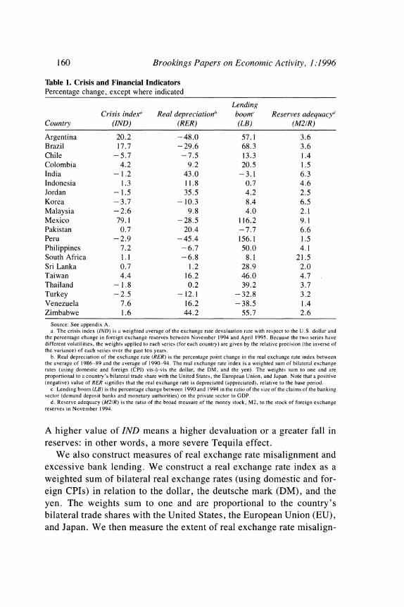
We measure the extent of financial crisis in 1995 with a crisis index (denoted IND) that measures pressures on the foreign exchange market. IND is a weighted average of the devaluation rate with respect to the U.S. dollar and the percentage change in foreign exchange reserves between the end of November 1994 and the end of each of the first six months of 1995. For each country, the two series have different vola- tilities. Accordingly, the weights that we apply to each series for each country are given by the relative precision of each series over the past ten years. 2 The rationale for this index is as follows. If capital inflows reverse, the government can let the exchange rate depreciate. Alterna- tively, it can defend the currency by running down reserves or by increasing interest rates. Since there are no reliable and comparable cross-country interest rate data, we construct the index using levels of reserves and exchange rates. The values for IND are listed in table 1.
12. Similar indexes have been used by Eichengreen, Rose, and Wyplosz (1995) for the case of Europe, by Frankel and Rose (1996) to study currency crises in developing countries, and by Kaminsky and Reinhart (1996) to study banking and balance of pay- ments crises. Barro (1995) and Calvo and Reinhart (forthcoming) use the stock market index to measure the extent of the financial crisis.
160 Brookings Papers on Economic Activity, 1:1996
Table 1. Crisis and Financial Indicators Percentage change, except where indicated
Lending Crisis index' Real depreciation" boom" Reserves adequacy"
Country (IND) (RER) (LB) (M21R)
Argentina 20.2 -48.0 57.1 3.6 Brazil 17.7 -29.6 68.3 3.6 Chile -5.7 -7.5 13.3 1.4 Colombia 4.2 9.2 20.5 1.5 India -1.2 43.0 -3.1 6.3 Indonesia 1.3 11.8 0.7 4.6 Jordan -1.5 35.5 4.2 2.5 Korea -3.7 -10.3 8.4 6.5 Malaysia -2.6 9.8 4.0 2.1 Mexico 79.1 -28.5 116.2 9.1 Pakistan 0.7 20.4 -7.7 6.6 Peru -2.9 -45.4 156.1 1.5 Philippines 7.2 -6.7 50.0 4.1 South Africa 1.1 -6.8 8.1 21.5 Sri Lanka 0.7 1.2 28.9 2.0 Taiwan 4.4 16.2 46.0 4.7 Thailand -1.8 0.2 39.2 3.7 Turkey -2.5 -12.1 -32.8 3.2 Venezuela 7.6 16.2 - 38.5 1.4 Zimbabwe 1.6 44.2 55.7 2.6
Source: See appendix A. a. The crisis index (IND) is a weighted average of the exchange rate devaluation rate with respect to the U.S. dollar and
the percentage change in foreign exchange reserves between November 1994 and April 1995. Because the two series have different volatilities, the weights applied to each series (for each country) are given by the relative precision (the inverse of the variance) of each series over the past ten years.
b. Real depreciation of the exchange rate (RER) is the percentage point change in the real exchange rate index between the average of 1986-89 and the average of 1990-94. The real exchange rate index is a weighted sum of bilateral exchange rates (using domestic and foreign (CPI) vis-a-vis the dollar, the DM, and the yen). The weights sum to one and are proportional to a country's bilateral trade share with the United States, the European Union, and Japan. Note that a positive (negative) value of RER signifies that the real exchange rate is depreciated (appreciated), relative to the base period.
c. Lending boom (LB) is the percentage change between 1990 and 1994 in the ratio of the size of the claims of the banking sector (demand deposit banks and monetary authorities) on the private sector to GDP.
d. Reserve adequacy (M2IR) is the ratio of the broad measure of the money stock, M2, to the stock of foreign exchange reserves in November 1994.
A higher value of IND means a higher devaluation or a greater fall in reserves: in other words, a more severe Tequila effect.
We also construct measures of real exchange rate misalignment and excessive bank lending. We construct a real exchange rate index as a weighted sum of bilateral real exchange rates (using domestic and for- eign CPIs) in relation to the dollar, the deutsche mark (DM), and the yen. The weights sum to one and are proportional to the country's bilateral trade shares with the United States, the European Union (EU), and Japan. We then measure the extent of real exchange rate misalign-
Jeffrey D. Sachs, Aaron Tornell, and Andres Velasco 161
ment by measuring the percentage change in the real exchange rate index from the average of 1986-89 to the average of 1990-94.' This change variable is termed RER. A positive value of RER signifies that the real exchange rate is depreciated relative to the base period, while a negative value signifies appreciation relative to the base period. We expect that the Tequila effect will strike countries with a low value of RER. Although this way of measuring misalignment is common in the literature, it has serious shortcomings, such as not controlling for long- run productivity changes or terms-of-trade shocks that can shift the long-run value of RER. 4 In defense of our approach, we are trying to identify countries that experienced extreme overvaluations during a span of four years. If our index indicates a real appreciation of the order of 30 to 60 percent, it is very unlikely that this was caused by a pro- ductivity shock as opposed to a misalignment. The values for the percentage change in the real exchange rate index are also listed in table 1.
The weakness of the banking sector cannot be assessed directly, by comparing ratios of nonperforming loans to total assets, because, to the best of our knowledge, there exists no broad cross-country set of com- parable bank balance sheets. Hence we rely instead on an indirect measure of the vulnerability of the financial system: the magnitude of the increase in bank lending between 1990 and 1994. We presume that when bank lending expands very sharply during a short period of time, banks' ability to screen marginal projects declines, so that they are more likely to end up with a large share of weak borrowers in their portfolios. High risk areas, such as credit cards and consumer and real estate loans, tend to grow disproportionately in such lending booms. In addition, particularly in developing countries, the limited oversight capacity of the regulators is soon overwhelmed. Thus a bank lending boom is likely to produce a banking sector portfolio that is extremely
13. We take the average of the real exchange rate from 1990-94 as the end point, instead of the rate in 1994, in order to capture the idea that in a country that has had an overappreciated currency for a longer period, firms in the tradeable sector are more likely to have exited. Thus the longer the period of real appreciation, the greater the real exchange rate devaluation needed to bring about a given improvement in the trade balance. Moreover, none of the twenty countries in our sample, except Venezuela, experienced a sharp nominal depreciation during the first eleven months of 1994.
14. In the case of Mexico, Warner (1996) computes the equilibrium exchange rate controlling for these factors.

162 Brookings Papers on Economic Activity, 1:1996
vulnerable to the vagaries of the business cycle. 15 To identify cases of lending boom, we first measure the size of the banking sector's claims on the private sector, BIGDP, where B denotes bank loans to the private sector. (We include the claims of demand deposit banks and monetary authorities.)'6 We then look at the percentage change in this ratio be- tween 1990 and 1994, which we denote as LB = [(BIGDP),9941 (B/GDP)990] - 1. We assume that countries with a very large increase in bank lending are cases of lending booms (LB high), and therefore, vulnerable banking sectors. The values for LB are listed in table 1.
If, in a time of capital inflow reversal, the central bank is not willing to let the exchange rate suffer a sharp depreciation, it must be prepared to cover all its liquid liabilities with reserves. These liabilities include not only direct liabilities-the monetary base-but also the liquid lia- bilities of commercial banks, which can be withdrawn quickly. If the central bank does not intervene in a run on banks, bankruptcies could easily follow. Given the well-documented aversion of governments to bank bankruptcies, the larger the liquid bank liabilities, the larger the contingent claims on the central bank. Therefore, as argued by Calvo, the correct yardstick with which to evaluate the abundance of reserves is a broad measure of money, such as M2, compared with the stock of foreign exchange reserves. In the empirical analysis below we use the ratio of M2 to foreign exchange reserves (M21R) in November 1994 as the indicator of reserve adequacy. The values for this ratio are listed in the last column of table 1.
Since we are interested in countries that were exposed to international capital flows, we consider the countries in the Emerging Stock Markets Factbook of the International Finance Corporation. This sample con- sists of the emerging markets in which foreigners can invest in stocks and other financial instruments with relative freedom. We exclude tran- sition economies (China, Hungary, and Poland), countries that belong to the EU (Greece and Portugal), and Nigeria, for which there are no data available for claims on the private sector. Our resulting sample consists of twenty countries: Argentina, Brazil, Chile, Colombia, India, Indonesia, Korea, Jordan, Malaysia, Mexico, Pakistan, Peru, the Phil-
15. See Rojas-Suarez and Weisbrod (1995) and Gavin and Hausmann (1995). 16. We do not include nonbank financial institutions because these data are not
available for all the countries in our sample.

Jeffrey D. Sachs, Aaron Tornell, and Andre's Velasco 163
ippines, South Africa, Sri Lanka, Taiwan, Thailand, Turkey, Vene- zuela, and Zimbabwe.
To compute the real exchange rate indexes, we calculate the trade weights from the Direction of Trade Statistics of the International Mon- etary Fund (IMF). For the countries with multiple exchange rates, we obtain data on parallel exchange rates from the World Currency Year- book and the Country Reports on Economic Policy and Trade Practices published annually by the U.S. Congress. The rest of the data are from the International Financial Statistics (IFS) cd-rom. For the cases in which data are missing from the IFS, we use current country sources and the Recent Economic Developments country studies from the IMF. In each case, we check that the data are compatible with the available IFS data.
As shown above, if a country has a strong banking sector and a real exchange rate that is not very overvalued, then even if capital inflows were to reverse, expected depreciation would be below the threshold that induces investors to flee from the country. Therefore when a coun- try has sound fundamentals, investors will not attack it. Similarly, if fundamentals are weak but M21R is low, there will not be a speculative attack. In other words, a speculative crisis arises only when both fun- damentals and reserves are vulnerable.
To implement the model, we classify countries as strong or weak on fundamentals and reserves by ranking them with regard to RER, LB, and M21R. We first use a broad classification, under which most coun- tries are deemed to be in the region where a self-fulfilling attack is possible. We then restrict the definition, so that fewer countries are classified as being in the vulnerable region, and observe-how the results change as we alter the classification. In the broader classification, a country has strong fundamentals if its real depreciation is in the highest quartile of the sample and its bank lending boom is in the lowest quartile. Otherwise, a country has weak fundamentals and is presumed to be vulnerable to a self-fulfilling attack. We create a dummy variable for weak fundamentals, such that DWF is equal to one for weak funda- mentals and equal to zero for strong fundamentals. Similarly, a country has high foreign exchange reserves if its ratio of M2 to reserves is in the lowest quartile of the sample. Otherwise, we consider its reserves to be in the danger zone. Thus the dummy variable for low reserves,

164 Brookings Papers on Economic Activity, 1:1996
DLR, is equal to one for countries above the bottom quartile for the money-to-reserves ratio and equal to zero otherwise.
These definitions of DWF and DLR cast a wide net. They deem thirteen of the twenty countries vulnerable to a self-fulfilling reversal of capital inflow: Argentina, Brazil, Indonesia, Jordan, Korea, Malaysia, Mex- ico, the Philippines, South Africa, Taiwan, Thailand, Turkey, and Zim- babwe. The seven countries deemed not vulnerable are Chile, Colom- bia, India, Pakistan, Peru, Sri Lanka, and Venezuela. Below, we consider increasingly stringent definitions of the two dummy variables and show that our results are relatively robust to this modification.
The basic equation regresses the crisis index, IND, on the levels of RER and LB, taking into account the strength or weakness of these fundamentals and the adequacy of foreign exchange reserves. The main idea is that the effects of RER and LB on IND should be nonlinear, and should be large only when both DWF and DLR are equal to one. We implement this idea by estimating the equation in the following form:
IND = J3 + 2(RER) + 3(LB) + 34(DLR x RER) + 35(DLR X LB) + 36(DLR x DwF X RER)
+ 37(DLR x DWF X LB) + E.
The coefficients f2 and 33 capture the effects of the fundamentals on the crisis index in countries with high reserves (DLR = 0) and strong fundamentals (DWF = 0). According to our model, these coefficients should be zero. The effects of the fundamentals on the crisis index in countries with low reserves (DLR = 1) but strong fundamentals (DWF
= 0) are given by 32 + 34 and 33 + 35. Our model again predicts that J2 + I4 = 33 + J5 = 0. That is, countries with strong funda- mentals are not likely to suffer an attack, even if they have low reserves. Last, 32 + 34 + 16 and 13 + J5 + 37 capture the effects of the fundamentals on the crisis index in countries with low reserves and weak fundamentals. In these countries, we expect ,B2 + 34 + ,B6 to be negative: a more devalued real exchange rate as of November 1994 should lead to a smaller value of IND in 1995. Conversely, we expect ,B3 + ,B5 + ,B7 to be positive: a larger bank lending boom should lead to a larger value of IND in 1995.
Table 2 presents the results of the regression as we vary the terminal month of the dependent variable over a period of six months (from

?N ) r--
t- r
t (f) (f (f i o6
- 6 CO CO C-
' m ;
os~~~~~~~~C _- rs 0rs r r - m m 011 o 0 u : u:m_ o 1=
w f} r-o )- - o, ? Pt -o O O O O0,r
4n~~~~~~~~~~~~~~~~zC
Cn oN > > > > m m > > t m q~~~~00 C 00 tf 00 -004 -1 W- )2 .2 q
o _ - m Csv t- t- t- o) o 0S "C r- tf O t-to C) o , C
.~~~~~~~~~~~~~~~~~~~~~~~ 0 C\ m ?N O ,C ?m - W) m OOO :rn
t~~~~~~~~~~~~~~~~~~~~~~~" C.t
Sv . > ? ? ~ O ? N ? N ~ 00 t OO O "CO ZO .- _
Q 2 < ?<3 ?<3~~~~~~~~~~~
"C _ l ItI_ 3=
c;~~ ~ ~~~~~~~~~~ "C W) e0 c
> 22 I c o <~~~~~~~~~~~~~~~~~~~~~~~~~~~~~~~~~~~~~~~~~~~~~~~~~~~~~~~~~~~~~IIt-'
su oZ~~~~~~~~~~~~~~~~~~~~~~~~~~~
u~~~~~~~~~~~~~~~~~~~~~~~~~~~~~~~~~~~~~~~~~~~~~~~~~~c u LwC
z~~~ <= = = = 1

166 Brookings Papers on Economic Activity, 1:1996
January through June 1995). The relative effects on the three categories of countries just described are as expected. The sign of each set of coefficients stays constant across the six cases. In order to evaluate alternative hypotheses regarding the causes of financial crises in the next section, we use as a benchmark the crisis index for the period November 1994 through April 1995. For countries with low reserves and weak fundamentals, RER and LB enter the regression equation with the expected signs: the point estimate of 32 + ,B4 + 36 is - 2.65, and that of ,B3 + 35 + ,B7 is 3.83. Wald tests indicate that the hypotheses that 32 + P4 + 36 = 0 and P3 + ,35 + ,B7 = 0 can be rejected at the 10 percent significance level (their p values are 0.07 and 0.04, respectively). As can be seen from the table, these hypotheses can also be rejected for the periods from November through March and Novem- ber through May. As expected, RER and LB do not affect the likelihood of an attack in countries with low reserves but strong fundamentals: the estimates of ,B2 + ,B4 and ,B3 + ,35 are not significantly different from zero at the 10 percent significance level (Wald tests of the hypotheses ,B2 + 1X4 = 0 and ,B3 + 3 5 = 0 have associated p values of 0.72 and 0.12, respectively). The same is true for the other five periods. Last, in contrast to the zero values that we would expect, the estimates of ,B2 and ,B3 are positive and significantly different from zero at the 5 percent and 10 percent level, respectively, for the periods ending in April, May, and June. These estimates correspond to the four countries with high reserves in our sample (Chile, Colombia, Sri Lanka, and Venezuela).
The regression results support the idea that the level of central bank reserves, relative to short-term liabilities, is important in determining whether a country is vulnerable to a self-fulfilling panic. An interesting case in point is the comparison of Mexico and Peru. Both countries experienced a sharp real appreciation (29 percent and 45 percent, re- spectively) and a lending boom (116 percent and 156 percent, respec- tively), but only Mexico scores high on the crisis index. The difference is that Peru did not have low foreign exchange reserves, relative to M2. Specifically, in Peru the ratio of M2 to reserves was only 1.4, while in Mexico the ratio was 9. 1.
Table 2 shows that during the first six months of 1995, between 51 percent and 71 percent of the variation in the crisis index was explained by movements in the real exchange rate, the lending boom, and the dummies. This suggests that contagion was not random. The Mexican

Jeffrey D. Sachs, Aaron Tornell, and Andres Velasco 167
crisis was mainly contagious to countries with low reserves that had experienced real exchange rate appreciations, or steep increases in bank lending to the private sector, or both, during 1990-94.
If we fit a simpler equation that uses only a dummy variable for foreign exchange reserves, instead of the equations presented in table 2, we obtain similar results. For the period from November 1994 through April 1995, the fitted equation (with standard errors in paren- theses) is
IND - -18.29 - 1.93(RER) + 3.66(LB) (28.39) (1.12) (1.65)
+7.06(RER x DHR) - 2.36(LB x DHR), R2 = 0. 65. (2.42) (1.39)
To make the interpretation easier, we use a dummy variable for high reserves, DHR = 1 - DLR. It follows that the coefficients on RER and LB correspond to countries with low reserves. Thus the second and third coefficients show that in such countries, a higher real appreciation and a larger lending boom increase the crisis index.
The regression results are robust to changes in the definition of the dummy variables. Table 3 presents the regression results for different definitions of the dummies. The sign and significance of the estimates of P2 + 43, j3 + 15, j2 + j4 + P6, and P3 + j5 + j7 remain the same as in the benchmark equation if we add one or two countries to each of the high reserves group, the low lending boom group, and the low appreciation group. If we add three more countries to these groups, the only change is that the estimate of j2 + j4 + 36 becomes insignificant. Also, the results are not affected if we eliminate one country from each of the high reserves group, the low lending boom group, and the low appreciation group.
Moreover, our regression results are not driven by a single country. Table 4 presents the regression results when we eliminate from the sample one country at a time out of those with the largest changes in their crisis indexes. In each case, the sign and significance of the esti- mates of 12 + 14, 13 + 15, 12 + 14 + 16, and 13 + 15 + 17 remain essentially the same as in the benchmark equation.
It is interesting to note that the percentage change in M21GDP be- tween 1990 and 1994 does not perform as well as the lending boom

-ci ~~~~~~t N \C " O W)C -00 00 en N\.000N --
0C- e r- l, 0 01 - CI '
-c--- f -o ooo o00 "c- -o- t CI icl ON I) en~ 1)0 00
C1)0 01)0 (.)o ~ ci 0 ri) oNoo1- 10 1 0-c-- c- 1 o f ) - 1. "D6 - - 0-0
0 u 010
') 0- O00 C) )r-I C I 0~0 O)r- 00O r- r-i If)c- c oll, CI -of-- -of' 0 c ) O)ct-0 10of c)ll 0 C-I) of0CI c I) 0 ) >011-
-ofc r-W) - 1 )0 0
0 01 01.01C! lc 0 0 0 0 - 0
00 ON or- O)oc O) c- -ojo ocO-) 0"o O)o00 ciI 0 o -of riO) ) NC 0 r- -- -of-, 0cl, 111- c-I) -of O) f) O) 0 1
01~~~~~~~~~~~~~~~~~~~~~~~~~~~
~~ ci- o~01 CIA 00- WI) NOCr c~n ' 1)Oc c-1 )0 It 00 CII 00_o
11)010 di r Of - C~IA) Oc ON Oc. nc- 0 If')-
r-1616ci C - 16 icli 11o ct ci- 06 6 6 6 6 6 Eo.
I I I <~~~~~~~~~~~~~~~~~~~~~~~~~~~~~a
00:zN Oof110 c-If) 1)1) 00 N-I) 001
I 01~~~~~~~~~~~ I~~~~.-' .0 ~~~~~~~~~~~~~01~~~
0 r
O <.01>1~~~~~~~~~~~~~~~Z< = =<

7J ON r- r- ON r- \.c r- ON ON 00 \C CIA ON \C r- 00 It m c-A c-A oo w-) oo r- c) c;N w-) Z c) c-A r- r- WI) 00 C) C) C
ON m tn tn' rli tn' cl; M' rli 0 O' M'
Izu r- C-A r- C-A C-A 00 00
llc "P 17 17 r! ,I: O O m tn C-A W-) C-A "D m C-A oo
CL
u
C
ol 11-0 00 ol CIA m
rn c-A c-A W') 01-1 CIA 00 00 CIA
C-i 116 cl cl 00'
00 00 110 00 It m CIA 00 W') 00 r- 00 CIA Izu CIA 't 00 0,-, 't r- o", 00 CIA - ,C W') 0,-, 01-1 It r- 00 CIA
r- 01-1 01-1 r- 00 110 m C) 01-1 oll, 110 Izu
0c) ('4 00 0c) CIA r- ON 00 CIA W')
00 C-A 00 W-) C-, "t 110 tn
r- oo w c-A o6 4 r-: 4 r o6 4 6 6
It 00 00 01-1 01-1 WI) It 110 110 ON C) WI) ON 00 CIA WI) 00 ON WI) r- C-A C-A C) C-, 00 00 "C C-, C)
00
(:;N 00 00 00 cq r- 00 M
rl
C< C<
x x x x
u
<= <= <= U
+ + + + = 0
CA CA m m Z <= <= <= <= Lz

170 Brookings Papers on Economic Activity, 1:1996
variable (LB, measured as the percentage change in BIGDP). If we replace our lending boom variable by the percentage change in M21 GDP in the benchmark regression, the point estimate of ,B2 + ,B4 + 36 would be negative but insignificantly different from zero. The point estimate of ,B3 + ,35 + ,B7 would be positive but insignificantly dif- ferent from zero. Moreover, the R2 statistic for this regression is 0.29, down from 0.69 in the regression using the lending boom variable. This reflects the fact that M21GDP is a broader measure of liquidity (or financial deepening) that need not be correlated with the degree of bank vulnerability. Bank vulnerability seems to play the more important role in determining a country's vulnerability to crisis in 1995.
The finding that a high ratio of M2 to reserves is helpful in predicting the extent of a financial crisis lends some support to the Calvo hypoth- esis that central banks implicitly must be prepared to defend currencies against the overall stock of liquid monetary assets. A high ratio of M2 to reserves makes countries more vulnerable to speculative attacks. Similarly, the finding that real exchange rate appreciation increases the likelihood of a financial crisis echoes the argument of Rudiger Dorn- busch, Ilan Goldfajn, and Rodrigo Valdes. ' However, this finding should be qualified: the real exchange rate only has a powerful effect when a country's reserves are low, relative to the stock of money.
Other Possible Determinants of Financial Crises
There are several alternative hypotheses in the literature regarding the vulnerability of an economy to capital flow reversals. Many of these are supported by case-study comparisons of the experiences of a few countries, but their broader applicability is less clear. In what follows, we consider a handful of these hypotheses and evaluate their broad explanatory power. First, using multiple regression analysis, we check whether any of them help to explain the variability of IND, after con- trolling for RER, LB, and M21R. Second, we compare their predictions with the experiences of eight countries: Argentina, Mexico, and the Philippines (which fared badly); and Chile, Colombia, Indonesia, Ma- laysia, and Thailand (which fared well).
17. Dornbusch, Goldfajn, and Valdes (1995).

Jeffrey D. Sachs, Aaron Tornell, and Andres Velasco 171
Excessive Capital Inflows Make a Financial Crisis More Likely
In its simplest form, this view argues that what comes in must even- tually go out: large capital inflows today may (but need not) lead to large outflows tomorrow. Its implications are weighty if, as argued by Calvo, Leonardo Leiderman, and Carmen Reinhart among others, cap- ital flows are largely exogenous to emerging markets, so that a sudden flight may be triggered by circumstances far beyond policymakers' control.'8 Some developing economies (for example, Korea in the 1960s) have taken in large amounts of foreign capital over long periods of time with few harmful effects, but it is alleged that this occurred in periods of much more stable capital flows. In today's world of fickle private capital movements, it is argued, large inflows leave a country exposed to the latest mood of Wall Street traders.
To explore whether this view is supported by the data, we add to our benchmark regression the average ratio of capital inflows to GDP from 1990 to 1994, alone and interacted with the low reserves dummy and the low reserves and weak fundamentals dummy (we denote the corre- sponding coefficients by 138, 139, and ,B10, respectively). We estimate this regression imposing two restrictions: 132 + 134 = 0 and 133 + 135 = 0. As can be seen from table 5, the estimates of 138, 139, and 1310 are insignificant. Moreover, we cannot reject the null hypotheses that 138 + 139 = 0 and 138 + 139 + P130 = 0. We obtain the same results when we include the percentage change in capital inflows as a share of GDP between 1990 and 1994 (table 6). Thus, if the level of capital inflows influences the likelihood of financial crisis, it probably does not do so directly, but rather, by affecting the real exchange rate and bank lending.
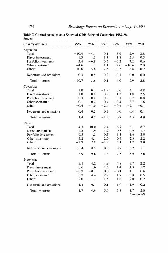
Moreover, the hypothesis that high capital inflows make a financial crisis more likely does not fare well in our subsample of eight countries, as can be seen from table 7. True, troubled Mexico's capital inflows in 1989-94, measured by the average capital account surplus (including errors and omissions) of 5.6 percent of GDP, may seem risky, but this pales in comparison to the 9.9 percent and 10. 1 percent surpluses posted by Malaysia and Thailand (arguably the Asian economies least affected by the Tequila shock), respectively, and the 6.3 percent posted by Chile (Latin America's star performer during this period). In fact, the regional
18. Calvo, Leiderman, and Reinhart (1994).

- o > m o~~~~C o t -t o i
Cll
OC rn r-w
zt rI > W) 00 0 't x ?m U < o x o t o v o m x o t ckl~~~~~~~~~7
r . - S x t - o t m > o N t -~~~~~~~~~~~~~~~~~~~~~~C .2 F%- - ? x - o - o o o o c c~~~~~
x ?:D~~~~~~~~~~~~~ k Ow~~~~~~~~~~~~~~~~~~~c
rA w) c
00~ ~ ~ "C rnrA -
+ _ S G . ?0
BJ~~~~~~~~- VJ *' _ o
_ -,Z O r O X N 3.
MS~~~~~~~~~c S EtX m 4 4> b N oe.
A- O ^' _ t O m N m O O O O C Q~~~~~~~~~~~~~~~~~~~~~~~~-t
eS q w ::n~~~~~~~~~~~~~~~~~~Q v X Q ? Q~~~~~~~~~~~~~~~~~~C Q ti _ _ _ D q s O~~~~~~~~~~Q
Qn OC O r~~~~~~~~~~~~~~~~~~~C _4 Z

o o W) 'IC rn 0 0 0 (ON W)
0 0 O rq 'IC V) rli r- o o o o +
V) W)
o o "t 4 V) 4 r- V) rn
Z
oc, V) r- W) C4 C14 00 'IC CZ Ci 0 ON 'IC 'IC 00 CD C14
0 0 V) (ON V) W) 00 CZ
CZ ct E
CZ 4 > v
v cq -tp a,
14i lc (ON 0 C14 00 00 00 00 C14 00 en 1. t) - en o kf) 'tt 00 r- CD
CZ
CZ
CZ CZ
r- (ON OC (ON (ON CZ W) OC W) W) (ON >
ci
7D
4j 00 00 (ON 00 'IC 00 00 C14 0 re) (ON - 00 re)
CZ 4j CZ
CZ CZ >
E ct E
CZ C
v CZ v
CZ v C
10- V) UU ul
C'S x x
CZ 14i CZ
> O >
ci.. a, v CZ CZ
-C
Z-10 C 00 oo oo C
Z <= <=
174 Brookings Papers on Economic Activity, 1:1996
Table 7. Capital Account as a Share of GDP, Selected Countries, 1989-94 Percent
Country and item 1989 1990 1991 1992 1993 1994
Argentina Total -10.4 -4.1 0.1 3.9 2.9 2.8 Direct investment 1.3 1.3 1.3 1.8 2.5 0.5 Portfolio investment 3.4 -0.9 0.3 -0.2 7.2 0.6 Other short-runL -4.6 1.1 1.1 2.6 -10.6 2.0 Other" -10.6 -5.6 -2.5 -0.3 3.8 -0.2
Net errors and omissions -0.3 0.5 -0.2 0.1 0.0 0.0
Total + errors -10.7 -3.6 -0.1 4.0 2.9 2.8
Colombia Total 1.0 0.1 -1.9 0.6 4.1 4.8 Direct investment 1.0 0.9 0.8 1.3 1.8 2.5 Portfolio investment 0.3 0.0 0.2 0.1 0.7 0.8 Other short-runL 0.1 0.2 -0.4 -0.4 3.7 1.6 Other" -0.4 -1.0 -2.4 -0.4 -2.1 -0.1
Net errors and omissions 0.4 0.2 0.7 0.0 0.4 0.1
Total + errors 1.4 0.2 -1.3 0.7 4.5 4.9
Chile Total 4.3 10.0 2.4 6.7 6.1 8.7 Direct investment 4.5 1.9 1.2 0.8 0.9 1.7 Portfolio investment 0.3 1.2 0.5 1.1 1.6 2.0 Other short-runL 3.2 4.1 2.0 0.9 2.3 2.2 Otherh -3.7 2.8 -1 .3 4.1 1.2 2.9
Net errors and omissions -0.4 -0.5 0.9 0.7 -0.2 -1.1
Total + errors 3.9 9.6 3.3 7.5 5.9 7.6
Indonesia Total 3.1 4.2 4.9 4.8 3.7 2.2 Direct investment 0.6 1.0 1.3 1.4 1.3 1.2 Portfolio investment -0.2 -0.1 0.0 -0.1 1.1 0.6 Other short-run!, 0.7 4.4 2.2 1.7 -0.8 0.5 Otherh 2.0 -1.1 1.5 1.8 2.0 -0.2
Net errors and omissions -1.4 0.7 0.1 -1.0 -1.9 -0.2
Total + errors 1.7 4.9 5.0 3.8 1.7 2.0 (continued)

Jeffrey D. Sachs, Aaron Tornell, and Andre's Velasco 175
Table 7. (continued) Percent
Country and item 1989 1990 1991 1992 1993 1994
Malaysia Total 3.4 4.1 11.8 15.0 17.0 2.1 Direct investment 4.4 5.4 8.5 8.9 7.9 6.2 Portfolio investment -0.3 - 0.6 0.4 - 1.9 - 1. - 2.3 Other short-run" -0.1 -0.5 2.1 2.7 -1.4 1.0 Other" -0.7 -0.3 0.9 5.3 11.5 -2.8
Net errors and omissions -0.9 2.5 -0.3 0.1 5.4 -0.7
Total + errors 2.4 6.6 11.5 15.1 22.3 1.4
Mexico Total 0.5 3.4 8.7 8.1 9.2 3.4 Direct investment 1.5 1.1 1.6 1.3 1.2 2.1 Portfolio investment 0.1 - 1.6 4.2 5.7 7.7 2.0 Other short-run" -0.4 -0.4 0.1 1.8 -0.5 -1 .4 Other" -0.7 4.4 2.8 -0.8 0.7 0.6
Net errors and omissions 2.2 0.5 -0.8 -0.3 -0.9 -0.4
Total + errors 2.7 3.9 7.9 7.8 8.3 2.9
Phillipines Total 3.2 4.6 6.4 6.1 5.6 7.7 Direct investment 1.3 1.2 1.2 0.4 1.4 2.9 Portfolio investment 0.7 - 0.1 0.2 0.1 -0.3 -0.7 Other short-run!, 0.1 0.9 1.8 -0.3 1.0 0.9 Other" 1.1 2.7 3.2 5.9 3.5 4.6
Net errors and omissions 0.9 1.3 -0.3 -1.0 0.5 0.3
Total + errors 4.1 6.0 6.1 5.1 6.1 8.1
Thailand Total 9.1 10.6 11.9 8.8 9.0 9.9 Direct investment 2.4 2.7 1.9 1.8 1.2 0.1 Portfolio investment 2.1 0.0 -0.1 0.8 4.4 1.7 Other short-run!, 2.2 4.6 5.6 3.2 1.1 -1.7 Other"' 2.5 3.4 4.5 3.0 2.3 9.7
Net errors and omissions 1.3 1.7 0.4 -0.5 -0.2 -1.1
Total + errors 10.4 12.3 12.3 8.3 8.7 8.8
Source: International Monetary Fund, Balance of Pai 'vinens Slialislic.s for all countries except the following: Argentina 1994: IMF, Ar-geniliinta-Rec enii E-ono,no1ic- DevelopmnenIs ( 1995); Colombia 1993-94: Inter-American Development Bank's worldwide web page.
a. "Other short-run' is constructed by identifying short-term flows within the category 'other investments'" in the IMF's standard presentation of the capital account.
b. "Other" is constructed as a residual.

176 Brookings Papers on Economic Activity, 1:1996
average of capital inflows for Latin America (3.2 percent) is substan- tially below that of Asia (7.3 percent). And dividing the countries into those strongly influenced by the Tequila effect (Argentina and the Phil- ippines, in addition to Mexico) and those less so, we find that, on average, the latter enjoyed a larger capital account surplus (6.2 percent) than the former (3.6 percent). '9
It Is the Composition of Capital Inzflows That Matters
This hypothesis comes in two varieties. The first emphasizes that short-term flows (equities, short-maturity bonds, and deposits in local banks) can turn around easily, while longer-term flows (long-maturity bonds and loans, and especially, foreign direct investment) cannot. The second focuses on the effects of each kind of flow: long-term capital inflows such as foreign direct investment are good because they increase the productive capacity of the country and produce the revenues nec- essary to cover future capital outflows (if they occur), while short-term flows may be associated with consumption booms or inefficient invest- ment projects.20 However, both varieties of the hypothesis have the same flavor: foreign direct investment is desirable; "hot" (that is, short- term) money is not.
To determine whether this dichotomy is important, we add to the benchmark regression, one at a time, the average ratio of short-term capital inflows (defined as the sum of portfolio investment, other short- term flows, and errors and omissions) to GDP from 1990 to 1994, and the percentage change in this variable between 1990 and 1994. As can be seen from table 5, the average ratio of short-term capital inflows does seem to matter (with marginal statistical significance) for the pre- diction of financial crises in countries with low reserves and weak fundamentals (the hypothesis that 18 + 19 + 1310 = 0 is rejected with a p value of 0.09). However, as can be seen in table 6, the percentage
19. Our results on the composition of capital inflows are related to those of Claes- sens, Dooley, and Warner (1995).
20. The link with inefficient investment projects can be rationalized in the following way. If domestic banks are borrowing abroad and lending this money at home, they will be unwilling to finance long-term investment projects with short-term borrowing, pre- ferring to direct the resources to more liquid credit card or consumption loans. And if, in fact, these resources end up in the hands of a domestic real investor, the investor must be willing to finance a project with short loans-a high risk strategy that could reveal something about the quality of the management or the project.
Jeffrey D. Sachs, Aaron Tornell, and Andres Velasco 177
change in short-term capital inflows does not enter significantly. Fur- thermore, when fundamentals are strong, neither the average nor the percentage change cnter significantly.
In the subsample of eight countries, the evidence that short-term capital inflows matter is weaker. As can be inferred from table 7, the "gang of three" troubled countries (Argentina, Mexico, and the Phil- ippines) received, on average, a smaller share of GDP in the form of short-term inflows (1.4 percent) than did the relatively untroubled na- tions (2.2 percent). Within Latin America, unscathed Chile actually absorbed more hot money (3.5 percent of GDP), on average, than did collapsing Mexico (2.9 percent). These are averages over 1989-94, and it could be argued that with short-term flows only the last year is significant. But this consideration scarcely changes the conclusions. If one considers 1993 (1994 is already tainted by the shock in some countries), the average of short-term inflows for the countries that later came under attack (Argentina, Mexico, and the Philippines) is 1.4 percent of GDP, while for the other countries it is 3.0 percent.
Large Current Account Deficits during the Period of Inflows Make a Financial Crisis More Likely
In the case of Mexico, the large and growing current account deficit has often been singled out as a key determinant of the crisis.2' This story has two strands. In one, large deficits lead to high external debt until the country either becomes insolvent (the present value of con- ceivable trade balance surpluses does not suffice to cover external ob- ligations) or faces a borrowing constraint (lenders understand that the country will have no incentive to repay any additional debt).22 In either case, lending ceases, and the country finds itself in a crisis. The second strand stresses that even when insolvency or credit limits are not ini- tially at issue, large external deficits expose a country to the fickleness of capital markets. If investors suddenly decide to stop financing its deficits, the country must undergo a sudden and painful adjustment. If, in addition, this adjustment creates severe economic disruption (labor
21. Dornbusch and Werner (1994) stressed this point even before the collapse; Dornbusch, Goldfajn, and Valdes (1995) have stressed it since.
22. Atkeson and Rios-Rull (1996) emphasize the role of borrowing constraints in the case of Mexico.

178 Brookings Papers on Economic Activity, 1:1996
unrest, the need to levy highly distortionary taxes, and so forth), ex post, the country may have difficulty paying, thus validating the pes- simistic expectations of investors. In this case there would be multiple equilibria. 23
The recent experience of Mexico has stimulated such concerns, but can one generalize the link between large current account deficits and vulnerability to financial crises in other emerging markets? Malaysia and the Philippines are instructive examples. As can be seen from table 8, those countries' current accounts were large and variable over the last decade. During 1989-94, Malaysia's average deficit was reasona- bly high: 4 percent of GDP, as compared to Mexico's 5.4 percent. It was also extremely variable, increasing from 2 percent of GDP in 1990 to almost 9 percent in 1991, falling for a couple of years, and then rising to almost 6 percent in 1994. Malaysia is not unique among Asian countries in this regard. Over 1989-94, the average current account deficit for an Asian country in the smaller sample was 4.1 percent of GDP; the corresponding figure for a Latin American country was 2.1 percent. Over the same period, the average external deficit for Argen- tina, Mexico, and the Philippines was 3.5 percent of GDP, while for the five countries that were not hit by crisis it was 2.9 percent-which is not enough of a difference to account for the variation in depth among the financial crises that occurred in early 1995.
Regressions for the larger sample of emerging markets tell a similar story. In tables 5 and 6 we include in the benchmark regression the average ratio of the current account to GDP from 1990 to 1994 and the percentage change in this ratio over the same period, alone and inter- acted with the low reserves dummy and the low reserves and weak fundamentals dummy (we again denote the corresponding coefficients by 38, 19, and I 10, respectively). Again in this case, we cannot reject the null hypotheses that 18 + 19 = 0 and 18 + 19 + 310 = 0. The same is true for the percentage change in the ratio of the current account to GDP for the period 1990-94.
Even if change in the current account does not seem to matter, do its components have an independent effect?24 A plausible view is that
23. See Calvo (1995) for such an explanation of the Mexican case. 24. As Feldstein and Horioka (1980) point out, saving and investment are highly
correlated in the medium run, even in environments in which one might expect a high degree of capital mobility (for example, industrialized countries). This point is even

Jeffrey D. Sachs, Aaron Tornell, and Andres Velasco 179
Table 8. Current Account as a Share of GDP, Selected Countries, 1989-94 Percent
Country and item 1989 1990 1991 1992 1993 1994
Argentina Current account - 1.7 3.2 -0.3 - 2.9 - 2.9 - 2.8
Investment 15.5 14.0 14.6 16.7 18.2 19.9 Saving 13.8 17.2 14.3 13.8 15.3 17.1
Chile Current account -2.5 - 1.8 0.3 - 1.7 -4.6 - 1.5
Investment 25.5 26.3 24.5 26.8 28.8 26.8 Saving 23.0 24.5 24.8 25.1 24.2 25.3
Mexico Current account - 2.8 - 3.0 - 5.1 - 7.3 - 6.4 - 7.6
Investment 22.2 22.8 23.4 24.4 23.2 23.5 Saving 19.4 19.8 18.3 17.1 16.8 15.8
Colombia Current account -0.5 1.3 5.7 2.1 -4.2 -4.8
Investment 20.0 18.5 16.0 17.2 19.9 19.8 Saving 19.5 19.9 21.6 19.3 15.7 15.0
Philippines Current account -3.4 -6.1 -2.3 - 1.9 -6.0 -4.3
Investment 21.6 24.2 20.2 21.3 24.0 24.0 Saving 18.2 18.1 17.9 19.5 17.9 19.7
Thailand Curent account - 3.5 - 8.5 - 7.7 - 5.7 - 5.6 - 5.9
Investment 35.1 41.1 42.2 39.6 39.9 40.1 Saving 31.6 32.6 34.5 33.9 34.3 34.3
Malaysia Current account 0.8 - 2.0 - 8.9 - 3.7 - 4.4 - 5.9
Investment 28.6 31.3 35.9 33.5 35.0 38.5 Saving 29.4 29.3 27.0 29.7 30.6 32.6
Indonesia Current account - 1.2 -2.8 -3.7 -2.2 - 1.3 - 1.6
Investment 35.2 36.1 35.5 35.9 33.2 34.0 Saving 34.0 33.3 31.8 33.7 31.9 32.4
Source: International Monetary Fund, Iniiernialiotnail Finan11c1ial Sitilislics tor all countries except the following: Argentina 1994: IMF, Argeniinita-Rec enl1 E o,wo,nic Dev'elopmnens ( 1995): Colombia 1994: IMF, Colombhia-Receni Econom,ic De- veloptenes ( 1995); the Philippines 1994: IMF, Phili;;ines-Recenl Economic Develo;lmens ( 1995).

180 Brookings Papers on Economic Activity, 1:1996
a current account deficit caused by an increase in investment is of less concern (because productive capacity and hence the ability to repay debt are increasing) than one caused by a fall in saving. This view does not receive support from our regression analysis. As presented in tables 5 and 6, the average and percentage changes in the ratios of saving to GDP and investment to GDP for the period 1990-94 do not seem to explain why some countries suffered a financial crisis in 1995 and others did not.
Loose Fiscal Policy Lies behind Financial Crisis
Imprudent fiscal policy has often been singled out as a cause of financial and currency crisis in emerging markets, particularly in Latin America. A country's fiscal stance may matter directly; for instance, a large public sector borrowing requirement over time may lead to bal- looning public debt and investor discomfort. Perhaps more important, a fiscal deficit may underlie many of the often mentioned culprits of financial crisis, such as current account deficit, real appreciation, and high monetary growth. Any effect that these factors seem to have on the likelihood of crisis may actually be the result of fiscal policy.
As important as a country's fiscal stance may be in theory, however, it is important to notice that irresponsible fiscal behavior was not among the central causes of the recent troubles. In the case of Mexico, the government ran budget surpluses in 1992 and 1993, and a deficit of less than 1 percent of GDP in 1994; the country's public debt, at about 40 percent of GDP, was less than 60 percent of the OECD average.25 The same is true of Argentina (where in 1992-94 the deficit averaged 0.5 percent of output) and to a lesser extent of the Philippines (with an average deficit of 1.6 percent of GDP in the same period).26 Neverthe- less, fiscal performance was better, on average, in the countries that escaped crisis. For the period 1989-94 as a whole, the countries without
more relevant in the case of emerging markets, which are imperfectly integrated into world financial markets.
25. See Sachs, Tornell, and Velasco (1996a) for details and discussion. 26. Such numbers have to be interpreted with caution. Talvi (1996) stresses that in
the context of a consumption boom, any measure of the deficit that is not cyclically adjusted can be extremely misleading. This point seems to have some validity for Mexico and Argentina, where the recessions of 1993 caused incipient (and ultimately, substan- tial) deficits, making sharp fiscal adjustment necessary.

Jeffrey D. Sachs, Aaron Tornell, and Andres Velasco 181
crises show an average surplus of 0.6 percent of GDP, as opposed to the average deficit of 1.7 percent of GDP for Argentina, Mexico, and the Philippines. OnCe again, though, while these differences are not trivial, they are not large enough to account for the huge disparities in observed outcomes.
To check for the influence of fiscal policy more generally, in tables 5 and 6 we include as predictors in our regressions the average and percent change over the period 1990-94 in the ratio of government consumption to GDP. Only the percentage change in government con- sumption does seem to matter in the prediction of financial crisis, but once again, only in countries with low reserves and weak fundamentals (the hypothesis that 18 + 39 + 310 = 0 is rejected with ap value of 0.03). Government consumption does not enter significantly in the other cases. We do not perform a regression with the fiscal deficit because we lack comparable cross-country data for 1993 and 1994.
The Crucial Real Exchange Rate
As the results presented above show, a big share of the cross-country variation in the crisis index is explained by variations in the real ex- change rate and in the patterns of bank lending in the 1990s, and by the ratio of reserves to monetary assets. It is natural to ask what accounts for the changes in these variables. In this section we focus on the behavior of the real exchange rate in our subsample of eight countries. The following section deals with the genesis of the bank lending booms.
The conventional wisdom is that capital inflows and outflows (and terms-of-trade shocks) explain much of the short-run variation in the real exchange rate. The standard story is that capital inflows stimulate overall absorption, so that the demand for both traded and nontraded goods must rise. If the economy is open, it faces a very elastic supply of tradeables at world prices. The supply of nontradeables, on the other hand, is much less elastic, reflecting the fact that resources have to be redeployed to the home goods sector if its output is to increase. The capital inflow, therefore, naturally increases the relative price of non- traded goods.
But this conventional wisdom does not fit well with the data. The most striking fact about the large sample of emerging markets-and

- I . t ON
x t * xS) x~~~~~~~~~~~~~~~~~~k) s0 0 kS) 010 'I 7E r -. I
X~~ ~~ i-Q ro o c
o c
o C
kr IA It I II
2 MD~~~~~~~~~~~~~~~~~~~~~~~~~~~~~~~~~~~~~~~~~~F t ( :, c l> un
X 3- Xc onri > 'S) O t- riri > N - su
CO
QCO4 c _mc
_ ~ ~ ~ ~ ~ ~ - .> 3 3
Y CES b b X N N O1~) s c -NI) X
Jeffrey D. Sachs, Aaron Tornell, and Andres Velasco 183
about our subsample of eight cases, in particular-is the lack of cor- relation between the size of capital inflows and real exchange rate behavior. In table 9 we classify countries according to the size of their real appreciation. The countries with the largest real appreciation (Ar- gentina and Mexico) experienced an average capital account surplus (that is, capital inflow) of 3.6 percent of GDP over 1990-94; for the countries in the middle group (Chile and the Philippines), the average surplus was 6.5 percent; and it was 6.7 percent for the countries with the least appreciation (Colombia, Indonesia, Malaysia, and Thailand).
There are three other generic explanations for the variation in the real exchange rate. First, similar capital inflows might lead to different changes in absorption (and therefore to differences in the demand for nontradeables) across countries. Second, although the resulting changes in absorption might be similar, structural differences across countries might make the associated price responses differ. Third, in the short run, nominal exchange rate policy may limit the extent of appreciation, even if fundamentals have changed. We consider each explanation in turn.
Similar Capital Inflows Lead to Different Changes in Absorption
One possibility is that capital comes in, but the inflow does not lead to additional demand for goods and services. This could happen for several reasons. We focus on two: the sterilization of inflows and an offsetting fiscal contraction.
In theory at least, a country with an active central bank could simply buy up the inflow, leaving demand unchanged. The balance of payments identity is helpful to see this point: CA + AR = KA, where CA is the current account, KA is the capital account, and AR is the change in the level of reserves. If the whole of the capital account surplus goes into reserve accumulation (AR = KA), the current account need not regis- ter a deficit. In practice, however, a sterilization of this magnitude- several percentage points of GDP per year-is not easily accomplished, since the associated costs can be quite high, in the form of central bank losses or the disintermediation of the banking system.27
27. Traditional open market operations (that is, the sale of bonds by the central bank) affect the central bank's balance sheet (higher foreign exchange reserves are matched by higher domestic bond liabilities), but ensure that the money base is un-

184 Brookings Papers on Economic Activity, 1:1996
All the countries in the crisis group (Argentina, Mexico, and the Philippines), except for Argentina, engaged in sterilization of some sort, but with differing intensities and degrees of success. All the Asian countries engaged in substantial open market operations, and all but Indonesia used reserve requirements in a countercyclical manner. In addition, Malaysia and Indonesia-along with Singapore and Taiwan (not in our crisis group)-moved around government deposits and pen- sion fund assets to lower deposits held by commercial banks. In Latin America, Chile and Colombia came close to the Asian modus operandi, implementing active sterilization on all fronts-in particular, early in the inflow period. Mexico is a peculiar case because it generously issued cetes and tesobonos as part of its open market operations, but then moved in the other direction by setting required bank reserves against peso deposits to zero. To summarize the evidence, differences in ster- ilization do not seem to account for the large differences in real ex- change rate outcomes.
Alternatively, domestic absorption might fail to rise in response to capital inflows because of countercyclical fiscal policy. Clearly, if a cut in the government deficit is of similar magnitude to an increase in private spending, aggregate demand will be largely unchanged. More important for our purposes, since government expenditure generally falls largely on nontraded goods, a cut in government spending in response to an increase in capital inflows will directly diminish excess demand in the nontraded sector, thus helping to limit increases in the real exchange rate.28 The behavior of government consumption in our
changed after a capital inflow. However, open market operations are fiscally costly because the bonds used to sterilize the money supply typically carry much higher interest rates than the central bank could earn by depositing the additional foreign exchange reserves abroad. A less direct kind of sterilization relies on changes in required bank reserves (and therefore in the monetary multiplier) to ensure that the money supply remains unchanged, even if the monetary base has risen. But here the problem is that high reserve requirements encourange disintermediation, and may cause financial activ- ity to curb markets over which the central bank has no control. Additionally, countries can attempt to prevent inflows from being intermediated by the domestic banking system (and thereby lent again) by requiring borrowers-in particular, public enterprises-to deposit loan proceeds with the central bank, rather than with commercial banks.
The literature on the mechanics and effects of sterilization has grown tremendously in the last couple of years. A few of the useful contributions are Calvo (1991), Reisen (1993), Frankel (1994), and Spiegel (1995).
28. Corbo and Hernandez (1994) stress this point.
Jeffrey D. Sachs, Aaron Tornell, and Andre's Velasco 185
sample does provide evidence that the countries that contracted fiscal expenditures experienced less appreciation. As table 9 shows, Mexico, in the group with the highest appreciation, expanded government con- sumption by an average of 0.8 percentage point of GDP between the period 1986-89 and the period 1990-94.29 For countries in the middle group, government consumption was approximately constant (as a share of GDP) between these two periods, while for the countries with the least appreciation, it fell by 3.9 percentage points of GDP.
Differences in Structure
Another reason why Asia and Latin America might differ with re- spect to real exchange rate movements is the differences in the under- lying productive structures of their economies. An argument in favor of this explanation might go as follows. In Latin America the tradeables sector is very resource intensive, while the nontradeables sector is more labor intensive. Therefore a change in the relative prices of nontrade- ables and tradeables would be required to induce a movement of labor between the two sectors. When demand for nontradeables rises (for example, because of a capital inflow), an increase in the relative price of nontradeables accompanies the flow of labor from tradeables to non- tradeables. In East Asia, by contrast, where tradeables manufactures are largely labor intensive, a flow of labor between nontradeables and tradeables can occur without sizeable movements in the price of non- tradeables relative to tradeables. In graphic terms, the production pos- sibility frontier between tradeables and nontradeables is nearly linear for Asian countries, while for Latin American countries, it is strongly bowed outward. If this view is correct, the real exchange rate in Latin American countries would be highly sensitive to shifts in domestic absorption caused by changes in capital inflows. In Asian countries, the real exchange rate would hardly vary with capital inflows.
One implication of this hypothesis is that, after controlling for other more conventional sources of variability, the real exchange rate should be less volatile in countries with large, labor-intensive tradeables sec- tors. To see whether there is evidence to support this hypothesis, we estimate regressions using the same sample of countries as in the pre-
29. No information is available on the behavior of government consumption in Argentina.
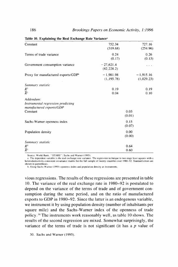
186 Brookings Papers on Economic Activity, 1:1996
Table 10. Explaining the Real Exchange Rate Variancea
Constant 752.34 727.16 (319.68) (254.96)
Terms of trade variance 0.24 0.26 (0.17) (0.15)
Government consumption variance -27,621.4 (82,228.2)
Proxy for manufactured exports/GDP" - 1,981.98 - 1,915.16 (1,195.78) (1,029.23)
Slu,nnary statistic R_2 0.19 0.19 R2 0.04 0.10
Acddenidwl/n: Inistrumenztcil regressioni predicting inanqftwctured exI)orts!GDP Constant 0.03
(0.01)
Sachs-Warner openness index 0.15 (0.07)
Population density 0.00 (0.00)
Slu mnnariy stcatistic R2 0.64 R2 0.60
Source: World Bank. "STARS': Sachs and Warner (1995). a. The dependent variable is the real exchange rate variance. The regression technique is two-stage least squares with a
heteroskedasticitv-consistent covariance matrix for the full sample of twenty countries over 1980-92. Standard errors are shown in parentheses.
b. Using Sachs-Warner ( 1995) openness index and population density as instruments.
vious regressions. The results of these regressions are presented in table 10. The variance of the real exchange rate in 1980-92 is postulated to depend on the variance of the terms of trade and of government con- sumption during the same period, and on the ratio of manufactured exports to GDP in 1980-92. Since the latter is an endogenous variable, we instrument it by using population density (number of inhabitants per square mile) and the Sachs-Warner index of the openness of trade policy.3' The instruments work reasonably well, as table 10 shows. The results of the second regression are mixed. Somewhat surprisingly, the variance of the terms of trade is not significant (it has a p value of
30. Sachs and Warner (1995).

Jeffrey D. Sachs, Aaron Tornell, and Andre's Velasco 187
0.18). The variance of government consumption has the wrong sign and is insignificant. Most important for our purposes, the share of manufactured exports in GDP has the expected sign (a higher ratio means less variability for the real exchange rate), but has a p value of 0. 12. When we run the same regression eliminating the variance of government consumption as a regressor (given the poor performance of the fiscal variable), the p value falls to 0.08. Thus there is weak evi- dence to suggest that the larger a country's tradeables sector, the lower the variability in its real exchange rate resulting from fluctuations in world interest rates and domestic demand.
Nominal Exchange Rate Policy
The explanations discussed so far have focused on the degree to which the equilibrium real exchange rate changes in response to capital inflows and other fundamentals. An alternative line of explanation fo- cuses not on the underlying fundamentals, but on the degree to which nominal exchange rate policy can prevent the real exchange rate from appreciating, even if the underlying equilibrium relative price of non- traded goods has changed. This is what the policy of "real exchange rate targeting" seeks to achieve."3
Most economists would agree that if the capital inflow, and therefore the change in the "fundamental" real exchange rate, are more or less permanent, real exchange rate targeting cannot succeed in the long run: repeated nominal devaluations will simply elicit repeated increases in prices and will fail to affect the real exchange rate. But as usual, definitions of the long run vary widely. If there is enough price sticki- ness over plausibly short periods, and if capital inflows are also short- lived, so that a brief period is all that is at stake, then nominal exchange rate policy may well have some ability to prevent real appreciation.32
31. Those who advocate such policy would probably prefer to say that since capital inflows are typically transitory, they do not change the long-run equilibrium real ex- change rate. Hence real exchange rate targeting simply attempts to keep the current real exchange rate from deviating too far from its "'long-run level."
32. Calvo, Reinhart, and Vegh (1995) make a different point concerning the poten- tial virtues of targeting: even if it is inflationary, it may improve welfare. Consider a standard maximizing model in which domestic money is held because of a cash-in- advance constraint. Suppose that the foreign nominal (but not the real) interest rate falls temporarily. If domestic policy is static, consumption and the current account will undergo a welfare-reducing fluctuation. If, by contrast, the rate of nominal exchange

188 Brookings Papers on Economic Activity, 1:1996
The evidence from our subsample of eight countries is instructive as to the effects of real exchange rate targeting. Indonesia, Colombia, and Chile have explicitly attempted to target the real exchange rate. An important aspect of policy in these three countries was not simply to attempt to target some arbitrary and constant real exchange rate, inde- pendent of circumstances. Both Colombia and Chile explicitly cited changing fundamentals (oil in Colombia, higher flows of foreign direct investment in Chile) as reasons for allowing nominal and real appreci- ation at several junctures over the five-year period. Note, also, that these attempts at targeting were not without cost: in the 1990s Chile and Colombia experienced slower convergence to international inflation rates than did Mexico and, especially, Argentina, in spite of their vir- tuous fiscal policies. The same is true of Indonesia in comparison with Thailand and Malaysia. To summarize, an accommodating nominal exchange rate policy may be able to limit real appreciation over the short to medium run, although probably at some expense, in terms of inflation.
Lending Booms, Banking Crises, and Currency Crises
Our empirical work suggests that the countries that experienced lend- ing booms were more likely to suffer currency crises as a result of the Tequila effect. In this section we examine why this might be so, and ask why some countries experienced lending booms while others did not.
The observation that banking and currency difficulties often go hand in hand is hardly new: the link has been evident in crises ranging from the United States in the 1930s to Chile in the early 1980s.33 Theoreti-
rate depreciation is temporarily increased to offset the foreign shock, domestic con- sumption will be flat, the current account will remain balanced, and welfare will not fall. l
33. Wigmore (1987) argues that the failure of the Federal Reserve to protect the U.S. banking system in the winter of 1932-33 was the result of its fear that providing lender-of-last-resort credit to the banks would undermine the U.S. dollar's link to gold. In Chile in 1982, high interest rates under a fixed exchange rate helped to precipitate a banking collapse. The associated expansion of domestic credit contributed to the demise of the exchange rate peg; see Velasco (1991) for details.

Jeffrey D. Sachs, Aaron Tornell, and Andres Velasco 189
cally, the link between these "twin crises" is not hard to ascertain. Abrupt changes in the demand for money (caused, for instance, by expectations of a devaluation and an incipient speculative attack) can cause a sharp fall in bank deposits. But under a fractional reserve system, banks do not have sufficient cash in hand to cover their liabil- ities: in the absence of an injection of liquidity from the outside (typi- cally from the central bank), it is very likely that payments will cease and a bank panic will occur. Even if the banks could wait until loans matured in order to satisfy depositors' demands (which would take time, given their essential role as maturity transformers), the ensuing adjust- ment would be neither easy nor painless. The resulting credit squeeze on borrower firms would send interest rates sky high. In emerging markets, banks are the main source of corporate credit, and most firms cannot turn around and borrow from the world market, no matter how deregulated the capital account may be. The need to avoid a wave of bankruptcies and serious economic disruption serves as yet another reason for the government to step in.
One implication of this situation is that the monetary base is not the only claim on the central bank that can be called in when times are bad. In fact, since bank liabilities are covered by implicit or explicit govern- ment guarantees, all M2 is potentially a liability of the central bank. Therefore the expansion of liquidity generated by a bank run can feed a speculative attack on the reserves of the central bank.
Bank portfolios can be weakened suddenly by an exogenous shock. But bad luck is not the only culprit of bank weakness. More often than not, portfolios are weakened endogenously by swift expansions of credit: boom leads to bust. As Michael Gavin and Ricardo Hausmann persuasively argue, the empirical link between lending booms and fi- nancial crises is very strong.34 Rapid growth in the ratio of bank credit to GDP preceded financial troubles in Argentina (1981), Chile (1981- 82), Colombia (1982-83), Uruguay (1982), Norway (1987), Finland (1991-92), Japan (1992-93), and Sweden (1991). Among the eight countries in our subsample, there was substantial lending growth during the period 1990-94 in Argentina, Mexico, and the Phillippines, which were the countries that experienced the greatest increases in their crisis
34. Gavin and Hausmann (1995).

190 Brookings Papers on Economic Activity, 1:1996
indexes during 1995. By contrast, Indonesia and Malaysia, which were much less severely affected by the Tequila shock, did not experience prior lending booms.
With regard to lending booms, it is extremely important to distin- guish levels of lending from rates of increase. All the Asian countries, except the Philippines, show very high ratios of private sector credit to output. This indicates nothing but financial deepening and, in and of itself, is no cause for concern. On the other hand, sharp increases in lending to the private sector within a short period of time are worrying. Such jumps are likely to lower average loan quality.
Why were there lending booms in some of the countries in our sample? A commonly cited culprit is swift liberalization of the capital account, followed by a surge in inflows that, presumably, was inter- mediated by the banking sector. There are two problems with this explanation. First, while there have been incremental moves toward liberalization in all of the countries in the sample, in almost all cases the capital account has been quite open for a long time. For instance, Indonesia liberalized its capital account in the 1970s, well ahead of its current account; Mexico, except for a brief period of controls during the 1982 crisis, has always remained open to capital movements. The two partial exceptions are Colombia and Chile, and even they have reasonably open capital accounts by any measure.35 Thus it is difficult to draw a clear link between an extreme policy change on the external front and a subsequent lending boom.
The second problem is that there is no obvious correlation between the size of the capital inflow and the subsequent behavior of bank credit. Such a correlation only seems to exist in the case of Mexico, where both capital inflows and bank lending grew tremendously. Malaysia and Chile, and to a lesser extent Colombia, experienced very large capital account surpluses that had no obvious effect on bank behavior.36
35. In both these countries the main restrictions are taxes on short-term inflows, which were instituted in the early 1990s. Chile also requires that portfolio flows remain in the country for at least one year.
36. Calvo, Leiderman, and Reinhart (1994) offer the intriguing conjecture that the composition of capital flows is important in this regard: foreign direct investment typi- cally is not intermediated by the banking system, while other flows are. To some extent, this may explain the bank behavior in Malaysia (where there had been a massive boom in foreign direct investment) and in Chile (which was among the countries that received the greatest increase in foreign direct investment in Latin America).

Jeffrey D. Sachs, Aaron Tornell, and Andre's Velasco 191
But if the liberalization of the capital account does not seem to have played a role in causing lending booms, domestic financial liberaliza- tion does appear to have been influential. Financial liberalization typi- cally is accompanied by aggressive behavior on the part of banks. In order to raise deposits, banks increase interest rates and fund more risky projects. Given the existence of deposit insurance (implicit or explicit), depositors find it profitable to move to these banks. Although the pur- pose of prudential regulation is to impede this tendency, during the early years of liberalization the capacity for oversight is usually poor. Consequently, when significant capital inflows take place in the early stages of financial liberalization, the lending boom that follows is likely to be associated with an increase in the riskiness and vulnerability of bank portfolios. Moreover, since lending expands rapidly, it is difficult to determine the ability to pay of borrowers who can repay old debts with easy credit. The weaknesses of the banking system do not surface until capital inflows reverse.
During the late 1970s and the 1980s, the progression from bank privatization and deregulation to lending boom to eventual bust was observed in a number of countries. In Latin America, Argentina, Chile, and Colombia went through this cycle.37 In Asia, the same was true for Indonesia and Malaysia.38 In Indonesia, for example, the cycle became evident in 1989-90, when financial liberalization was followed by a lending boom. In Mexico the privatization and deregulation of the banking system in the early 1990s had a similar effect.
The type of deregulation that a country implemented also made a difference. For instance, Colombia launched a wide-ranging program to modernize its financial system in 1990.19 Barriers to entry were relaxed, reserve requirements were rationalized, and most (but not all) interest rates were freed. But at the same time, supervision was strengthened, and all banks were forced to comply with the capitaliza- tion standards of the Basel Accord. A country's policy stance was often determined by previous experience. In the early 1980s both Chile and Colombia experienced credit booms and financial crises that led to bank interventions, liquidations, and bailouts-at a substantial cost to tax-
37. See Balifo and Sundarajan (1991) for studies from a set of countries that includes Argentina, Chile, Uruguay, and the Philippines.
38. See Folkerts-Landau and others (1995). 39. See Edwards (1995).

192 Brookings Papers on Economic Activity, 1:1996
payers. The lesson of these episodes was deeply ingrained in the minds of policymakers, and in subsequent years both governments made the enhancement of bank supervision a priority. Bank problems following liberalization in Indonesia and Malaysia in the late 1970s and early 1980s also caused these countries to pay greater attention to bank oversight. The strong performance of all four countries in 1995 re- warded this policy emphasis.
During the period 1989-94, attitudes toward bank regulation and oversight varied widely across countries. There was no dichotomy be- tween laissez faire and thorough going interventionism-no country in our subsample subscribed to the latter in this period. Rather, some countries-Malaysia, Thailand, and to a lesser extent Indonesia, the Philippines, Colombia, and Chile-intervened at the margins to dis- courage those bank activities that were viewed as potentially too risky, and some did not. The Asian countries, in particular, instituted specific limits on commercial bank borrowing abroad and ceilings on domestic relending in areas such as consumer and real estate credits.4" All of these countries, to varying degrees, resorted to sterilization and changes in reserve requirements in an effort to limit credit growth. Sterilization seems to have been particularly important in Indonesia, Malaysia, and Thailand. In these countries, periods of aggressive sterilization coin- cided with low growth in bank assets, and periods of relaxation of sterilization coincided with rapid expansion.4"
A third possible cause of a lending boom is a recent stabilization episode. Deposits are highly correlated with money demand, and there- fore, with expected inflation. When a policy turnaround puts an end to hyperinflation, deposits swell, and so do bank loans. This effect, which is nothing but a beneficial payoff (greater financial intermediation) from
40. In Malaysia, measures to limit the credit-creating capacities of banks were instituted in 1993; in particular, restrictions on consumption credits, such as credit cards and credit for the purchase of motor vehicles. In Indonesia, the prudential regulation of commercial banks was tightened in 1991; in particular, by raising the required capital- to-assets ratio. Measures to discourage external borrowing, such as limits on commercial banks' foreign currency exposure and external loans, were also instituted. Thailand, too, created disincentives to foreign borrowing: in 1990 a 10 percent withholding tax on interest paid on foreign loans was reinstated (having been suspended for two years). In addition, the Thai authorities set limits on the relending capacities of banks, partic- ularly on loans for "nonproductive" activities, such as consumer and luxury real estate loans.
41. See Folkerts-Landau and Ito (1995).

Jeffrey D. Sachs, Aaron Tornell, and Andres Velasco 193
stabilization, probably explains some of the sharp increase in lending that occurred in Argentina, for example. It does not, however, explain the experience of Mexico, where stabilization occurred in 1988-89 but there was no increase in credit until 1991-94.
Conclusions
Are currency and financial crises the inevitable punishment for a country's misdeeds? Or are they simply prompted by contagion and animal spirits, striking guilty and innocent countries alike? In this paper we examine these questions by analyzing how twenty emerging markets fared in the face of the Tequila effect and its aftermath. Our main conclusion is that some degree of previous misbehavior was a necessary condition for crisis. This misbehavior took the form of overvalued real exchange rates and recent lending booms, coupled with low reserves, relative to the short-term commitments of the central bank. In the ab- sence of these fundamental weaknesses, contagion was at worst short- lived, and the Tequila effect left no hangover. At the same time, how- ever, an important element of self-fulfilling panic, or contagion, is evident in the aftermath of the Mexican crisis. Crises that could have occurred, did not, before the Mexican episode.
We also find that some common explanations for the occurrence of financial crises are not supported by the data from our sample. The behavior of current accounts, the size of capital inflows, and fiscal policy stances during the period 1990-94, in and of themselves, do not explain why some countries experienced greater financial crises than others in the aftermath of the December 1994 devaluation. Any explan- atory power that these variables do have is through their effect on the real exchange rate and credit to the private sector. For instance, the average current account deficit of hard-hit Argentina was 1. 1 percent, while the deficit of Malaysia (which did not experience a crisis) was 5.0 percent. Similarly, Argentina experienced capital inflows averaging only 1.2 percent per year, while in Malaysia, capital inflows averaged 11.4 percent.
Thus prudence in managing both exchange rates and banking systems seems to pay off. But this begs the question how overvaluation and lending frenzies can best be avoided. A striking fact in the data is that

194 Brookings Papers on Economic Activity, 1:1996
large capital inflows are associated with massive real appreciation in some countries, and with real depreciation in others. The Asian coun- tries, in particular, seem to have been able to absorb large quantities of foreign resources (as a percent of GDP) without experiencing sharp changes in relative prices. In part, this was probably related to their offsetting fiscal restraint. The performance of Chile, Colombia, and Indonesia seems to suggest that flexible and pragmatic management of the nominal exchange rate also matters. Finally, the underlying eco- nomic structure may play a role. We provide some preliminary evidence to suggest that countries with large, labor-intensive tradeables sectors find it easier to reallocate labor between tradeables and nontradeables without inciting massive shifts in relative prices.
Furthermore, large inflows of foreign capital need not cause a frenzy in bank lending and a growing stock of bad loans, as the experiences of Malaysia and Chile show. The domestic regulatory environment is more determinative of whether a crisis will occur, but here the policy questions are many. In particular, the capital adequacy and liquidity standards typically emphasized in developed economies may not be sufficient to regulate the volatile environment of emerging markets. Much more must be learned-and put into practice by vigilant regula- tors-in order to avoid further repetitions of the boom and bust financial cycle.
APPPENDIX A
Data
THIS APPENDIX describes the construction of the data presented in the text. Line references in parentheses are to the International Financial Statistics cd-rom.
Real Exchange Rate Depreciation
We use the percentage change in the weighted average of the bilateral real exchange rates (using CPIs) with respect to the yen, the dollar, and the DM as a proxy for real exchange rate depreciation. The weights

Jeffrey D. Sachs, Aaron Tornell, and Andres Velasco 195
sum to one and are proportional to the bilateral trade shares with Japan, the United States, and the European Union. The extent of depreciation is measured as the percentage increase in the real exchange rate index between its average during 1986-89 and its average during 1990-94. To construct the index, we compute the trade shares from the IMF's Direction of Trade Statistics (various years), and we use average nom- inal exchange rates (line rf from the IFS cd-rom) and CPIs (line 64). For countries with multiple exchange rates, we use the parallel rate. For Venezuela, our source is the periodical VenEconomy (Caracas: VenEconomia Distribuidores, various issues); for India, it is the World Currency Yearbook (Philip P. Cowitt, Brooklyn, N.Y.: International Currency Analysis, Inc.) for 1986-89 and the U.S. Congress's Country Reports on Economic Policy and Trade Practices for 1990-92. Since India abandoned its multiple exchange rate regime in 1993, for subse- quent years we use the official rate from the IFS cd-rom.
Lending Boom
For each year, we calculate the ratio of claims on the private sector by deposit money banks and monetary authorities (line 32d) to GDP (line 99b). When inflation is high, this ratio is biased upward because the available annual figure for claims on the private sector corresponds to the figure for December, while nominal GDP reflects the average price level over the entire year. To correct for this bias, we multiply the biased ratio by the ratio of the average price level to the price level for December. When inflation is low, this factor is basically equal to one. The variable used in the regression is the percentage change in this ratio from 1990 to 1994 (the period of capital inflows). Claims on the private sector for Indonesia are taken from Key Indicators of De- veloping Asian and Pacific Countries (Manila: Asian Development Bank, various issues) (hereafter, Key Indicators); and for South Africa, from the Quarterly Bulletin (Pretoria: South African Reserve Bank, various issues).
Ratio of M2 to Reserves
This ratio is calculated for November 1994. To obtain the figure for reserves, we convert total reserves minus gold (line 11) to national currency, using the average exchange rate for November (line rf). For

196 Brookings Papers on Economic Activity, 1:1996
M2, we use the sum of money (line 34) and quasi-money (line 35). For Indonesia, the value of M2 is obtained from Key Indicators, since the corresponding IFS series does not go beyond 1992.
Crisis Index
The crisis index is the depreciation rate of the real exchange rate plus the negative of the percentage change in reserves between November 1994 and a given month in 1995. Each of the two components is weighted by its precision (the inverse of the variance) over the sum of precisions. Precisions are calculated using ten years of monthly data. India and Venezuela had multiple exchange rates during part of this ten-year period. For India, we calculate the precisions using data start- ing in 1993, the year in which the country returned to a single exchange rate regime. For Venezuela, we calculate the precisions using data for the parallel rate starting in June 1994, when the country adopted a multiple exchange rate regime.
Current Account
The current account (line 78al) is converted to national currency using the annual average exchange rate (line rf). Current account data are not available for the following countries in the years specified: Argentina (1994), Colombia (1993, 1994), India (1993, 1994), Paki- stan (1994), the Philippines (1994), and Zimbabwe (1994). The missing data are obtained using the respective IMF Recent Economic Develop- ments (various years) for these countries. We measure the figure from the report as a share of GDP, and enter it in the regression in two different ways: as the average over the period 1990-94, and as the percentage change from 1990 to 1994. In the cases of India and Zim- babwe, since data are not available for 1994, we use 1993 as the end point.
Investment and Saving
To obtain measures of investment and saving, we use gross fixed capital formation (line 93e). We use other sources for Turkey, Zim- babwe, and India because national account data are not available for these countries in the IFS data base for all the years that we consider.

Jeffrey D. Sachs, Aaron Tornell, and Andres Velasco 197
For Turkey, we use data from the Organisation for Economic Co- operation and Development's National Accounts. For Zimbabwe, we obtain data from the World Bank's World Tables (Baltimore: Johns Hopkins University Press, various years). Data for 1994 are not avail- able for India and Zimbabwe. For these countries, we obtain the in- vestment and savings variables for that year using 1993 as the end point. Saving is constructed as the sum of investment and the current account.
Government Consumption
Government consumption is taken from line 91f of the IFS cd-rom. Since data are not available for Argentina, the country is excluded from the regression that includes this variable.
Capital Inflows
We construct this variable by adding the capital account (78bc), the financial account (line 78bj), and net errors and omissions (line 78ca). The sum is converted to national currency using the annual average exchange rate (we use the IMF's new definition of the balance of pay- ments; see the fifth edition of the Balance of Payments Manual). This measure of capital inflows is similar to the "old" definition of the capital account. Data are missing for Argentina (1994), Colombia (1993, 1994), India (1993, 1994), Pakistan (1994), the Philippines (1994), and Zimbabwe (1994). We use the respective IMF Recent Economic Developments (various years) for these countries to complete the series, although not even these data are available for India and Zimbabwe.
Short-Term Capital Inflows
The source for short-term capital inflows is the IMF's Balance of Payments Statistics. This variable is the sum of portfolio investment (line 4600 of this publication), errors and omissions (line 4998), and other short-term flows. The latter is constructed by identifying short- term flows within the category of "other investments" in the IMF's standard presentation of the capital account (lines 4727, 4733, 4734, 4768, 4771, 4777, 4789, 4792, and 4700).

198 Brookings Papers on Economic Activity, 1:1996
Taiwan
Taiwan is not included in any IMF or World Bank data base. Our main source for data on Taiwan is Key Indicators. However, monthly figures for reserves and the nominal exchange rate are from the Monthly Bulletin of Statistics of the Republic of China (Taipei: Directorate- General of the Budget, Accounting and Statistics, various issues) and various issues of the Economist.

Comments and Discussion
Guillermo A. Calvo: This is a very interesting paper that pulls together the various experiences associated with the infamous Tequila effect. It identifies three main factors that explain the depth of the crisis: an appreciated currency, larger than normal expansion in bank credit, and low levels of international reserves. As a yardstick for the adequacy of reserves, the authors select the ratio of M2 to foreign exchange reserves, not the conventional ratio of reserves to one month's worth of imports, the idea being that balance of payments crises take the form of a run against currency and are rarely associated with an import spree. Em- pirical estimates show that the first two factors have significant coeffi- cients if reserves are sufficiently low. Even more interesting, the paper argues that popular candidate factors like current account and fiscal deficits do not appear to be significant, confirming results obtained earlier by Jeffrey Frankel and Andrew Rose, and Graciela Kaminsky and Carmen Reinhart. '
The authors do not intend that their empirical results give a full explanation of the Mexican crisis or the Tequila effect. Rather, they test the hypothesis that the more vulnerable a country was before the Tequila episode, the more profound its crisis was likely to be. (The crisis index is a weighted average of devaluation and loss of interna- tional reserves after the Mexican crisis.)
I find myself in almost complete agreement with the point of view espoused in this paper, that balance of payments crises stem, first and foremost, from financial and structural vulnerabilities. The latter may
1. Frankel and Rose (1996); Kaminsky and Reinhart (1996).
199

200 Brookings Papers on Economic Activity, I :1996
be partially caused by flow disequilibria, but a balance of payments crisis may take place even though a country has been faithfully follow- ing IMF-type advice if, for instance, it has concentrated a large chunk of its domestic debt in short-run maturities (like Mexico's tesobonos). Furthermore, if they run a tight financial sector, countries can avoid balance of payments crises even though flow disequilibria are large, as has been the case in Peru. These results are important because they call into serious question a major tenet of the "Washington consensus" after the Tequila shock, namely, that economies that run current account deficits of more than 4 percent should be quarantined.
Turning to the empirical estimates, which constitute the heart of the paper, I feel that the variable for bank lending booms (LB) is well chosen. As Gavin and Hausmann show, an unusual expansion of bank credit foretells trouble.2 However, the role of the real exchange rate is much less clear. Japan's success was happily accompanied by a con- stantly appreciating currency. Why should Mexico have been different? There are models that explain why an appreciation may have very different implications in Japan than in a country like Mexico.
Suppose, for example, that a not fully credible trade liberalization is put into effect. Since individuals believe that this is a temporary policy, they will take advantage of present lower prices and prompt an expen- diture boom. The latter, in turn, is likely to induce a real appreciation of the currency. An expenditure boom, under some circumstances, can be socially costly and-independent of whether trade liberalization is continued or eventually abandoned-must come to an end; that is, it is not sustainable. Presumably, the "bad" appreciation is what bothers investors and may induce a run like that in Mexico. On the other hand, if the expenditure boom was associated with credible programs, the likelihood of such a run would be much smaller. The paper, however, makes no attempt to distinguish bad from good currency appreciations.
Consequently, I suspect that the real exchange rate effect reported in the paper may be a reflection of other factors, like credibility, and that it would be much more useful for policy purposes to try to identify these directly. In this respect, I suggest generating a variable that would capture the expenditure booms associated with bad currency apprecia- tion. If the real exchange rate appreciation is driven by a lack of cred-
2. Gavin and Hausmann (1995).
Jeffrey D. Sachs, Aaron Tornell, and Andres Velasco 201
ibility, individuals are more likely to expand consumption than invest- ment, especially than investment in highly durable goods, whose profitability depends on the nature of the trade regime. Thus consump- tion booms could be an appropriate indicator for bad and unsustainable currency appreciations.
The theoretical model discusses the pros and cons of a devaluation. According to the model, a devaluation is an effective pill against reces- sion. The idea is that devaluation facilitates an expenditure switch against tradables, and thus accommodates the decline in the current account deficit necessitated by capital outflows, without the need of a recession. But this Econ. 1 price effect ignores all the financial effects of a devaluation. In Mexico, for example, the banks had borrowed in dollars and, essentially, lent in pesos. Hence a successful devaluation that increased the real exchange rate might have resulted in a major negative shock in banks' balance sheets. This is not just idle thought: it appears to have been a major consideration behind the decision to prop up the Mexican peso after the crisis of December 1994. In Argen- tina, the disruption could have been many times larger. Therefore, I do not see a clear trade-off.
Turning to the metric used for reserves adequacy (the M2-to-reserves ratio or its inverse), a plausible alternative to the index employed in this paper would be to adjust the ratio of M2 to reserves by its first-log- difference standard deviation. In a related paper I find that Mexico displays a much higher standard deviation than Austria (by a factor of more than 4 to 1).3 Thus a ratio of M2 to reserves that would be considered dangerously high in Mexico is almost without risk in Austria.
A major puzzle that remains largely unanswered in this and other papers on the subject is why Mexico's output fell so sharply, despite massive international assistance, and why Argentina's unemployment grew to unprecedented levels (more than 18 percent), even though an open balance of payments crisis was prevented by the timely imple- mentation of an IMF program. If, as this paper suggests, financial muscle is a key factor in keeping a country from slipping into the abyss, why are the economies of Mexico and Argentina in such terrible con- dition? The paper suggests that the international assistance should have
3. See Calvo (1996).

202 Brookings Papers on Economic Activity, 1:1996
helped these countries to cushion the negative effects of a specula- tive attack. Was the assistance insufficient, or the IMF programs inadequate?
It is too early to tell. However, there is some evidence of both. For example, investors refused to roll over the tesobonos even after the Mexican package had been agreed on, and despite exceptionally high interest rates. A possible explanation is that the package had a clear time limit, it was temporary. If there had been no need for the funds to be disbursed, the treasury would most likely have declared victory and withdrawn its support. But this is not likely to have restored permanent stability to Mexico, because investors already knew that without the treasury the equilibrium would be bad. Hence the only credible path involved heavy use of foreign assistance. This explains the unwilling- ness to roll over Mexican debt despite the package, but why did interest rates remain so high?
This question requires explicit consideration of the associated IMF programs. The bottom line is that Mexico's current account deficit fell from 8 percent (as a share of GDP) to zero. This represents a major adjustment. Fiscal policy was strongly procyclical. Thus there is some evidence that the stabilization program itself may help to explain the sharp downturn in output. If this was foreseen by investors, it would likely be translated into a higher country risk factor, which would explain the high interest rates.
Was there any alternative? My short answer is, no. Relevant alter- natives would have involved much larger international assistance. This was not politically feasible. The courageous measures undertaken by the IMF and the treasury had already led them to the boundaries of their institutional mandates.
I conclude by highlighting some lessons from the approach taken in this paper, with special reference to emerging markets:4
-Debt structure is a key factor of macroeconomic stability. Short- term debt can induce crises based on self-fulfilling expectations. The type of debt holders also seems to matter. Domestic holders may attach a liquidity factor to domestic debt, either because the debt is interme- diated by banks or because it is being used in repos. This liquidity factor is likely irrelevant to foreign holders. Therefore large foreign
4. See also Calvo (1996).

Jeffrey D. Sachs, Aaron Tornell, and Andres Velasco 203
holdings of domestic debt may make its demand highly sensitive to expected net returns, and thus facilitate self-fulfilling prophesies.
-Domestic financial liberalization is desirable, but should be un- dertaken with a great deal of caution. Policymakers should keep a wary eye on sudden surges of bank credit, even though the credit is directed toward the private sector and interest rates are free. High bank reserves- to-deposit ratios, possibly with remunerated reserves, are advisable until monetary aggregates are stabilized.
-The choice of the exchange rate regime should take account of financial considerations (for example, the degree of currency substitu- tion, dollarization, the soundness of the banking system, and so forth). This prescription contrasts with the standard literature on this subject, which emphasizes aspects like the degree of price stickiness and the relative importance of nominal as against real shocks.
-Beware of false accounting. Appropriate measures of the fiscal deficit and the adequacy of reserves are hard to come by, and standard measures can be highly misleading. As Gavin and others and Ernesto Talvi have recently shown, emerging markets have highly procyclical fiscal revenues.5 Thus during a capital inflows episode, for instance, fiscal accounts may look deceptively healthy. For its part, reserves adequacy should be measured against all short-term government liabil- ities. These include not only M2 but all short maturity debt, independent of the currency denomination.
Richard N. Cooper: With Calvo, I like the basic thrust of this paper. My remarks focus on some quibbles and some observations stimulated by the paper.
The main results are built around the fitted equation that purports to give some explanation of what the authors call the crisis index, or to indicate the likelihood of a financial crisis. But what exactly is the nature of this fitted equation? Does it characterize the behavior of pri- vate actors? It is a peculiar formulation. Multiplying two variables in which there is some a priori interest is a bit arbitrary, particularly when one variable is defined as being in the upper quartile of a universe that is not fully explained. It raises the questions of how many experiments were run, and whether an effort was made to maximize the R2.
5. Gavin and others (1996); Talvi (1996).

204 Brookings Papers on Economic Activity, 1:1996
It reminds me of the early history of applied statistics in both the sciences and the social sciences. A lot of effort was devoted to curve fitting, to finding a curve that fits a particular set of data as well as possible. It is worth keeping in mind that while they use a sample of eight countries, the authors are basically addressing one episode- worldwide reaction to the Mexican crisis in the early months of 1995.
A normative or policy interpretation is possible. If the Brookings papers circulate as widely as many of us hope that they do, the financial community and governments around the world will discover this equa- tion and build their expectations around it. In future there will not be any financial crises of the type that occurred in early 1995, because governments will be sure to keep the variables above or below the thresholds indicated in this paper, and the private sector, observing that governments have done so, will behave properly. That can only be tested in the future. It would have been helpful, however, if the authors had tested this equation on at least one past episode that was not used to fit it. An equation fitted around a single episode does not give high confidence.
The most interesting results of the paper are the negative ones. The authors examine a number of hypotheses that have been broached in financial, policy, or academic circles, largely generalizations from this Mexican episode, and show that they do not stand up under close scrutiny in a wider universe. In particular, they look at the size of the current account deficit: 8 percent of GDP is often said to be too high for stability. The authors mention Malaysia as a nice counterexample. They could just as well have mentioned Hungary, although its govern- ment recently took major constrictive action. Peru's current account deficit is up in this range in 1996. Should the financial community worry seriously about Peru? The authors' equation clearly says no, so long as M2 is adequately low relative to reserves. The negative results are interesting and a little sobering; they warn against generalizing casually about the world from a single episode.
The authors draw the conventional, unfavorable comparison of booms based on consumption with booms based on investment. They argue that booms based on investment might not have such a large impact on the price of nontradeable goods because investment is largely composed of imported goods. I would like to challenge that assumption.
A large part of most investment booms is construction, and construc-
Jeffrey D. Sachs, Aaron Tornell, and Andre's Velasco 205
tion is quintessentially a nontradeable, except in those rare cases where whole teams of construction workers are imported from Korea or else- where. In contrast, the consumption boom in Chile in the late 1970s and early 1980s was largely in importable consumer durables. In these examples, it is measured investment, not consumption, that drives up the price of nontradeables. However, it is an artifact of accounting conventions that economists consider construction-particularly hous- ing construction-as investment, and purchases of consumer durables as consumption.
The authors write as though they know the relative price of nontrade- ables. I urge caution about identifying the "real exchange rate" as it is normally measured (and is here) with the relative price of nontrade- ables, and encourage attempts to approximate the latter directly, for example, by measuring the price of export goods for which supply is somewhat elastic relative to value-added prices in retail or construction. My guess is that there is only a weak correlation between such measures and that used by the authors, which involves consumer price index comparisons adjusted by market exchange rates.
In searching for determinants or predictors of financial crises, the authors curiously neglect history and reputation. I would have thought that the simplest and most straightforward explanation for why Mexico, Argentina, and Venezuela ran into trouble, while Thailand, Malaysia, and Korea did not, is that the former had run into trouble before, while the latter had knuckled down and handled their equally large negative shocks in a much smoother way. The latter countries, unlike the former, have no recent history of agonizing debt rescheduling combined with serious domestic pressure for outright debt repudiation.
Since the issue here is expectations, the most natural observation would seem to be that when countries are hit by a negative shock of some kind, modestly risk-averse investors-whether based in New York or London, or indeed in Mexico City, Buenos Aires, or Singapore- would hold on to their Thai and Malaysian investments but dump their investments in Mexico and Argentina and Venezuela. History and ex- perience and the associated reputations of these countries indicate that course of action. This obvious hypothesis is remarkably absent in the discussion, except insofar as it may be captured indirectly in some of the included variables.
Mexico provides the precipitating event in the episode under discus-
206 Brookings Papers on Economic Activity, 1:1996
sion, so it is worth noting that apparently it was Mexican residents, rather than foreigners, who dumped Mexican securities first and sold in large volume. Foreigners were still holding on after the assassination of presidential candidate Colossio and the other events of March 1994. Indeed, they continued to invest in Mexico through October, and to hold their assets even through November and most of December.
The formal model distinguishes between domestic and foreign hold- ers of assets, with an (unstated) assumption that foreigners are the more skittish. But it is usually the domestic holders that have the more nu- anced inside knowledge; such knowledge can be, and probably is, con- veyed to the major financial centers, but it is less likely to be absorbed by the decisionmakers there. The Mexican experience also serves as a warning not to look just at liabilities to foreigners, as is often done (but not here), when assessing the financial exposure of a country.
One of the big puzzles is that when the December 1994 peso deval- uation occurred, many members of the financial community seemed genuinely surprised-in spite of the fact that economists like Dorn- busch, John Williamson, and other members of the Brookings Panel had been saying for many months, "Mexico is in trouble. It is over- extended. It is financially fragile." The financial community simply did not believe the warnings, or the analysis underlying them.
Anyone who believes, or even uses, rational expectations should worry a lot about this particular episode. When Mexico did devalue, parts of the New York financial community expressed disbelief. It was inconceivable. The Mexicans could not do that. They had violated our trust-a false trust it turned out to be-regardless of the fact that many economists had been saying that devaluation was perfectly sensible and, in fact, sooner or later would be required. The Mexican episode under- lines the profound weakness of the typical assumption of rational ex- pectations, that all agents use the same model of the world, and that it is the correct model.
The Mexican episode and its associated Tequila effect also under- lines the well-known but little-understood point that any modern finan- cial system is basically a house of cards. Such a system necessarily involves maturity transformation, and therefore it relies on the law of large numbers: that is to say, independent, imperfectly correlated trans- actions. That is especially true for banks. But it holds for financial

Jeffrey D. Sachs, Aaron Tornell, and Andre's Velasco 207
markets in general, and it holds for financial markets in particular countries, such as Mexico and Argentina. When something signals all individual transactcrs to move in the same direction in the same short interval, the basic fragility of any financial system is revealed. This is not a new point; it has attracted the attention of economists since the early nineteenth century.
Finally, what, if any, policy guidelines can one draw from this ex- perience and from this paper? Obviously, countries have to follow good policies, but as this paper shows, following good monetary and fiscal policies is not by itself sufficient. In addition to good policies, they have to have a sound financial structure. Yet, as I have just indicated, in some fundamental sense there is no such thing as a sound financial structure that serves its economies well. Most financial structures are intrinsically unsound, in that a one-sided decision on the part of all agents can throw them into deep trouble. Can collective (governmental) actions reduce that prospect?
Two questions, in particular, need to be addressed. The first is whether countries such as the ones discussed here should integrate themselves more completely into the world financial market suddenly or gradually. For those who like hydraulic images, if the water in a blocked channel is at two different levels, should one remove the ob- stacle quickly, or should one first pump some water from the upper level to the lower level to slow the rush when the obstacle is finally removed? This is a live issue that many countries face. Should they liberalize capital movements in one go, as is being called for by mem- bers of the international financial community and, increasingly, by the international financial institutions? Or, should they maintain some brakes on capital movements until their economies are more thoroughly integrated into the world market, to avoid problems of huge financial surges? Or, are huge surges, in fact, less likely if integration is under- taken quickly?
The second policy issue is whether the international community should organize itself institutionally to deal with one-sided surges. An ad hoc package was put together for Mexico and, like Calvo, my own view is that under the circumstances, it was the right thing to do. The damage to real economies would have been much greater without it. But was the Mexican package a one-time solution, or should there be a

208 Brookings Papers on Economic Activity, 1:1996
financial lender of last resort on an international scale? And if so, how could it be organized so as to minimize perverse incentive effects both for private players and for national policymakers?
General discussion: The Mexican currency crisis of December 1994 figured prominently in the general discussion at the meeting. James Tobin asserted that the severity of the Mexican crisis was hardly justi- fied by government policies in the years leading up to the collapse of the exchange rate regime. He recalled that Mexico apparently received the standard punishment for a country running large budget deficits and with substantial monetary inflation when neither the budget deficit nor inflation were out of control at the time. He concluded that Mexico was punished for crimes it did not commit, and discussed the factors that might have contributed to the severity of its currency crisis. He noted that in previous Mexican currency crises, investors anticipated that the country might default on some of its international debt and took this into account when negotiating the terms of debt contracts. However, during the late 1980s and early 1990s, institutions like the IMF and a number of commercial and central banks worked to improve the cred- ibility of Mexico in the international financial community by recom- mending that it drop exchange controls. The Mexican government fol- lowed this policy advice, despite the fact that the market for its debt was known to be very thin under adverse economic conditions. Tobin argued that the abolition of exchange controls for countries like Mexico was premature, and noted that even some advanced European nations, like France, maintained restrictions on convertibility into the early 1980s. He concluded that developed countries bear some of the blame for the severity of the Mexican currency crisis because they rushed this and other underdeveloped countries into complete convertibility with- out allowing for a safety net in the form of limited exchange controls.
James Duesenberry agreed with Tobin that the benefits of unre- stricted capital movements to a country like Mexico, especially in the short run, are hardly worth the costs. He noted that the benefits of correctly lining up interest rates between the United States and Mexico are probably small, relative to the cost of sudden speculative shocks and their aftermath. But while he agreed that capital controls would, in principle, be one way of approaching this problem, he cautioned that these are hard to enforce in underdeveloped countries and therefore are

Jeffrey D. Sachs, Aaron Tornell, and Andre's Velasco 209
not a viable policy option. Duesenberry concluded that floating ex- change rates represent the credible alternative to a policy that pegs the peso against the dollar, while conceding that floating rates would leave a considerable amount of instability and uncertainty.
Alan Blinder observed that Mexico's decision to peg its currency against the dollar, even when such a policy was not fully credible because of its large current account deficit, was intended as a poison pill that would force Mexican policymakers to pursue stabilization pol- icies for fear that devaluation would destroy their credibility with for- eign lenders. Blinder emphasized that this represented a high risk strat- egy because the government could not credibly give up its option to devalue. International and Mexican investors recognized this, and when a worsening current account deficit made a devaluation increasingly likely, they moved their assets to short-term and very liquid invest- ments. As a result, just before the collapse of the peso there was an avalanche waiting to happen since a large number of investors were poised to withdraw from Mexico. In retrospect, Blinder concluded, the Mexican crisis is an example of a poison pill that backfired, since the pegged peso policy ultimately increased the severity of the crisis.
Takatoshi Ito and Benjamin Friedman discussed how the emergence of mutual funds as major players in international financial markets exacerbated the Mexican currency collapse. Ito noted that dedicated bond and equity funds barely changed their holdings during the crisis because the managers of these funds have an explicit mandate to be in a certain market, such as Mexico or Latin America. It was mainly global bond and equity fund managers who sold heavily during the crisis and bought assets in other, safer countries. Friedman cautioned that holding a security via an open-end mutual fund might give the owner the illusion of liquidity because he can redeem his shares with a phone call, and that this ease of redemption might have added to the severity of the peso collapse. He noted that a typical retail investor who holds an equity in Mexico or some other emerging market is probably well aware that he is in a highly illiquid market. By contrast, if this same investor were to hold a share in an open-end mutual fund that held Mexican equities, he might readily redeem his shares, thus forcing fund managers to sell illiquid securities. Ito added that the peso crisis might have been less severe had it not taken place during the Christmas week, when the market was particularly thin and fund managers were in the process of

210 Brookings Papers on Economic Activity, 1:1996
rebalancing their portfolios in time for their balance sheet reporting deadline of December 31, thereby adding to market volatility.
Among those who contemplated institutional changes aimed at pre- venting similar crises in the future, Gregory Mankiw doubted that a currency board alone would have protected Mexico from severe eco- nomic disruption. A currency board might have helped Mexico to avoid the peso crisis, but at the cost of severe disruption to the banking sector. He observed that while the foremost goal of any central bank must be the preservation of the unit of account, the health of the banking sector is also vital to the functioning of an economy. Therefore, the Mexican central bank really had two objectives in the period leading up to the crisis: the preservation of the unit of account and the continued solvency of the banking system. Mankiw maintained that joint implementation of a currency board and narrow banking, whereby demand deposits are fully backed by short-term liquid assets, might have satisfied both pol- icy goals of the Mexican central bank because the former would prob- ably have avoided an exchange rate crisis, while the latter would have made bank runs unlikely.
Laurence Kotlikoff suggested that it would be easier for Mexico simply to dollarize and get out of the business of having its own cur- rency altogether. He imagined that under these circumstances, Mexico would take the dollar as its currency and adopt all U.S. financial insti- tutions and regulations, such as deposit insurance. Kotlikoff explained that this move would eliminate a lot of uncertainty in financial markets and allow Mexico much improved access to international lenders. Rich- ard Cooper responded by noting that the value of retaining the peso is measured in seigniorage, which amounts to about 1.5 to 2 percent for a middle-income country such as Mexico. He emphasized that seig- niorage represents an important source of revenue for the Mexican government, especially since tax evasion and the secondary economy are substantial. To this, Mankiw responded that the seigniorage prob- lem could be resolved by ordering the U.S. Treasury to turn over to the Mexican government the extra seigniorage arising from the dollar's use in Mexico.
Commenting on the role of the Tequila effect during the peso crisis, Ito observed that a number of countries, including Argentina and Thai- land, instituted measures to shore up their currencies against speculative attacks as soon as the Mexican currency crisis began. The behavior of

Jeffrey D. Sachs, Aaron Tornell, and Andres Velasco 211
these and other countries could be described by a reaction function, and a country's success in fending off speculative attacks would depend on a threshold specific to each country. Ito reasoned that some countries might well have suffered devaluations in the wake of the December 1994 peso crisis if they had not had the time and the means to implement policies that kept them from crossing their thresholds. Ito also used the example of an emerging markets mutual fund to illustrate how the Tequila effect might work. Managers of a Latin American mutual fund might respond to a Mexican currency crisis by selling their holdings in other Latin American countries in order to raise cash with which to meet expected share redemptions. An emerging markets fund manager might react to a peso crisis by selling shares in Thailand and Hong Kong, and thus contagion might occur simply because of fund man- agers' behavior. Ito added that while he found such a Tequila effect plausible, he has not seen evidence of one.
A number of participants also discussed the extent to which markets anticipated the December 1994 peso crisis, and what could be inferred about investor rationality from the degree of surprise in financial mar- kets when the peso actually collapsed. In response to Cooper's formal comments, Mankiw thought it unlikely that the peso crisis casts doubt on the rationality of investors on Wall Street. While he agreed that investors consistently ignored economists, who were overwhelmingly predicting a currency crisis in the period leading up to December 1994, he observed that this may have been perfectly rational in light of the profession's track record. Cooper replied that investors' decisions to ignore economists might indeed have been perfectly rational. However, he noted that the extent of surprise on Wall Street when the peso collapsed is hard to reconcile with rationality, given that devaluation was seen as a sensible and necessary action by a wide variety of cal- culations, even at the time. Blinder reported that at the time of the peso crisis, a number of central bankers and private investors claimed that the volume of tesobonos was secret and unknown to them; this despite the fact that the tesobonos were issued in public auctions, and the quantities were announced every single time. Blinder thought this ex- perience a good illustration that market participants were not acting rationally at the time of the peso crisis. Ito emphasized that financial markets were completely surprised by the collapse of the peso. From conversations with market participants, he had learned that a great deal

212 Brookings Papers on Economic Activity, 1:1996
of trust was placed in the pronouncements of the Mexican government, and that many investors suffered substantial losses, having borrowed in dollars and lent in pesos. Velasco agreed that the peso's collapse was largely unanticipated, noting that in the months before the crisis, interest rate spreads between peso and dollar assets were very stable. Financial markets did not reflect a rising probability of devaluation in the months leading up to December 1994.

Jeffrey D. Sachs, Aaron Tornell, and Andre's Velasco 213
References
Atkeson, Andrew, and Victor Rios-Rull. 1996. "Balance of Payments and Borrowing Constraints: An Alternative View of the Mexican Crisis." Jour- nal of International Economics (forthcoming).
Balifno, Toma's J. T., and Vasudevan Sundarajan, eds. 1991. Banking Crises: Cases and Issues. Washington: International Monetary Fund.
Barro, Jason. 1995. "When the First Domino Falls." Unpublished paper. Harvard University (September).
Calvo, Guillermo A. 1991. "The Perils of Sterilization." International Mon- etary Fund Staff Papers 38(4): 921-26.
. 1995. "Varieties of Capital-Market Crises." Unpublished paper. Uni- versity of Maryland (April).
. 1996. "Capital Flows and Macroeconomic Management: Tequila Les- sons." Unpublished paper. University of Maryland (February).
Calvo, Guillermo A., Leonardo Leiderman, and Carmen M. Reinhart. 1993. "Capital Inflows and Real Exchange Rate Appreciation in Latin America: The Role of External Factors." International Monetary Fund Staff Papers 40(1): 108-51.
. 1994. "The Capital Inflows Problem: Concepts and Issues." Contem- porary Economic Policy 12(3): 54-66.
Calvo, Guillermo A., Carmen M. Reinhart, and Carlos A. Vegh. 1995. "Tar- geting the Real Exchange Rate: Theory and Evidence." Journal of Devel- opment Economics 47(1): 97-133.
Calvo, Sara, and Carmen M. Reinhart. Forthcoming. "Capital Flows to Latin America: Is There Evidence of Contagion Effect?" In Capital Flows to Emerging Markets, edited by Morris Goldstein. Washington: Institute for International Economics.
Claessens, Stijn, Michael P. Dooley, and Andrew Warner. 1995. "Portfolio Capital Flows: Hot or Cold?" World Bank Economic Review 9(1): 153-74.
Corbo, Vittorio, and Leonardo Hernandez. 1994. "Macroeconomic Adjust- ment to Capital Inflows: Latin American Style versus East Asian Style." Policy Research Working Paper 1377. Washington: World Bank (November).
Dornbusch, Rudiger, Ilan Goldfajn, and Rodrigo 0. Vald6s. 1995. "Currency Crises and Collapses." BPEA, 2: 1995, 2 19-70.
Dornbusch, Rudiger, and Alejandro Werner. 1994. "Mexico, Stabilization, Reform, and No Growth." BPEA, 1:1994, 253-97.
Edwards, Sebastian. 1995. Crisis and Reform in Latin America: From Despair to Hope. New York: Oxford University Press.
Eichengreen, Barry, Andrew K. Rose, and Charles Wyplosz. 1995. "Exchange

214 Brookings Papers on Economic Activity, 1:1996
Market Mayhem: The Antecedents and Aftermath of Speculative Attacks." Economic Policy 21 (October): 249-312.
Feldstein, Martin, and Charles Horioka. 1980. "Domestic Saving and Inter- national Capital Flows." Economic Journal 90(358): 314-29.
Folkerts-Landau, David, and Takatoshi Ito. 1995. International Capital Mar- kets: Developments, Prospects, and Policy Issues. Washington: International Monetary Fund.
Folkerts-Landau, David, and others. 1995. "Effect of Capital Flows on the Domestic Financial Sectors in the APEC Developing Countries." In "Cap- ital Flows in the APEC Region," edited by Mohsin S. Kahn and Carmen M. Reinhart. Occasional Paper 122. Washington: International Monetary Fund (March).
Frankel, Jeffrey A. 1994. "Sterilization of Money Inflows: Difficult (Calvo) or Easy (Reisen)?" Working Paper 159. Washington: International Monetary Fund (December).
Frankel, Jeffrey A., and Andrew K. Rose. 1996. "Currency Crashes in Emerg- ing Markets: An Empirical Treatment." International Finance Discussion Paper 534. Washington: Board of Governors of the Federal Reserve System (January).
Gavin, Michael, and Ricardo Hausmann. 1995. "The Roots of Banking Crises: The Macroeconomic Context." Unpublished paper. Inter-American Devel- opment Bank.
Gavin, Michael, and others. 1996. "Managing Fiscal Policy in Latin America and the Caribbean: Volatility, Procyclicality, and Limited Creditworthi- ness." Unpublished paper. Inter-American Development Bank (March).
Kaminsky, Graciela L., and Carmen M. Reinhart. 1996. "The Twin Crises: The Causes of Banking and Balance-of-Payments Problems." International Finance Discussion Paper 544. Washington: Board of Governors of the Fed- eral Reserve System (March).
Krugman, Paul. 1979. "A Model of Balance-of-Payments Crises." Journal of Money, Credit, and Banking 11 (3): 311-25.
. 1996. "Are Currency Crises Self-Fulfulling?" In NBER Macroeco- nomics Annual 1996, edited by Ben S. Bernanke and Julio Rotemberg. Cambridge, Mass.: MIT Press (forthcoming).
Obstfeld, Maurice. 1994. "The Logic of Currency Crises." Cahiers Econo- miques et Monetaires (Bank of France) 43: 189-213.
Reisen, Helmut. 1993. "Southeast Asia and the 'Impossible Trinity.' " Inter- national Economic Insights 4(3): 21-23.
Rojas-Suarez, Liliana, and Steven R. Weisbrod. 1995. "Financial Fragilities in Latin America: The 1980s and 1990s." Occasional Paper 132. Washing- ton: International Monetary Fund (October).
Sachs, Jeffrey D., Aaron Tornell, and Andres Velasco. 1996a. "The Collapse

Jeffrey D. Sachs, Aaron Tornell, and Andre's Velasco 215
of the Mexican Peso: What Have We Learned?" Economic Policy (forth- coming).
. 1996b. "The Mexican Peso Crisis: Sudden Death or Death Foretold?" Journal of International Economics (forthcoming).
Sachs, Jeffrey D., and Andrew Warner. 1995. "Economic Reform and the Process of Global Integration." BPEA, 1:1995, 1-95.
Spiegel, Mark M. 1995. "Sterilization of Capital Inflows Through the Banking Sector: Evidence from Asia." Working Paper PB95-06. Federal Reserve Bank of San Francisco, Center for Pacific Basin Monetary and Economic Studies (June).
Talvi, Ernesto. 1996. "Exchange Rate-Based Stabilization with Endogenous Fiscal Response." Working Paper 324. Washington: Inter-American Devel- opment Bank (March).
Velasco, Andr6s. 1991. "Liberalization, Crisis, Intervention: The Chilean Financial System, 1975-85." In Banking Crises: Cases and Issues, edited by Tomas J. T. Balinio and Vasudevan Sundarajan. Washington: Interna- tional Monetary Fund.
. 1995. "When Are Fixed Exchange Rates Really Fixed?" Unpublished paper. New York University (December).
Warner, Andrew M. 1996. "Was Mexico's Exchange Rate Overvalued in 1994?" Development Discussion Paper 524. Cambridge, Mass.: Harvard Institute for International Development (February).
Wigmore, Barrie A. 1987. "Was the Bank Holiday of 1933 Caused by a Run on the Dollar?" Journal of Economic History 47(3): 739-55.