Financial Conditions Indexes: A Fresh Look after the ... · Bruce Kasman (JP Morgan Chase ... A...

Financial Conditions Indexes: A Fresh Look after the Financial Crisisproceedings of the u.s. monetary policy forum 2010

The Initiative on Global Markets

the university of chicago booth school of business

The massive global movements of capital, products, and talent in the modern economy have fundamentally changed the nature of business in the 21st Century. They have also generated confusion among policymakers and the public. Chicago Booth School of Business (Chicago Booth) will continue our role as a thought leader on how these markets work, their effects, and the way they interact with policies and institutions.

The Initiative on Global Markets organizes our efforts. It supports original research by Chicago Booth faculty, prepares our students to make good decisions in a rapidly changing business environment, and facilitates the exchange of ideas with policymakers and leading international companies about the biggest issues facing the global economy.

The Initiative spans three broad areas:

❖❖ International business

❖❖ Financial markets

❖❖ The role of policies and institutions

By enhancing the understanding of business and financial market globalization, and by preparing MBA students to thrive in a global environment, the Initiative will help improve financial and economic decision-making around the world.

The Initiative on Global Markets was launched with a founding grant from the Chicago Mercantile Exchange (CME) Group Foundation and receives ongoing financial support from the CME Group Foundation and our corporate partners: AQR Capital Management, Barclays Bank PLC, John Deere, and Northern Trust Corporation.

Foreword2

U.S. Monetary Policy Forum 2010 Report: Financial Conditions Indexes: A Fresh Look after the Financial Crisis

3

References28

Appendix31

Comments by William C. Dudley56

Comments by Narayana Kocherlakota62

Comments on the Panel Discussion by Anil K Kashyap67

Comments on the Panel Discussion Comments Charles L. Evans71

Comments to the Panel Discussion by Daniel K. Tarullo78

Participant List84

Acknowledgements92

Table of Contents

2

Foreword

The U.S. Monetary Policy Forum (USMPF) is an annual conference that brings academics, market economists, and policymakers together to discuss U.S. monetary policy. A standing group of academic and private sector economists (the USMPF panelists) has rotating responsibility for producing a report on a critical medium-term issue confronting the Federal Open Market Committee (FOMC).

The 2010 USMPF panel includes private-sector members David Greenlaw (Morgan Stanley), Jan Hatzius (Goldman Sachs), Ethan Harris (Bank of America Merrill Lynch), Peter Hooper (Deutsche Bank), Bruce Kasman (JP Morgan Chase), and Kim Schoenholtz, as well as academic panelists Anil Kashyap (Chicago Booth), Frederic Mishkin (Columbia), Matthew Shapiro (Michigan), and Mark Watson (Princeton). Hyun Song Shin (Princeton) took temporary leave from the panel to serve as an advisor to the President of the Republic of Korea.

This volume reports the results of the fourth USMPF conference, held on February 26, 2010 in New York, N.Y. The conference, despite a blizzard that nearly shut the city was attended by over 100 central bankers, academics, business economists, and journalists. The meeting began with a presentation of this year’s report, followed by a luncheon address titled “Debt and the Aftermath of the Global Financial Crisis: Is This Time Different?” by Kenneth Rogoff, Thomas D Cabot Professor of Public Policy at Harvard University, and ended with a panel discussion.

The fourth USMPF report, “Financial Conditions Indexes: A New Look after the Financial Crisis” authored by Hatzius, Hooper, Mishkin, Schoenholtz and Watson, focuses on measuring the condition of the financial sector and determining how financial conditions might inform monetary policy decision-making. Following the authors’ presentation, William Dudley, President of the Federal Reserve Bank of New York, and Narayana Kocherlakota, President, Federal Reserve Bank of Minneapolis offered their comments. After the conference the Federal Reserve Bank of New York has agreed to take over the job of updating the index that was featured in the report.

This year’s policy panel was entitled “Financial Regulatory Reform” and was moderated by David Wessel, economics editor of the Wall Street Journal. The discussion featured presentations by Daniel Tarullo and Charles Evans, Governor of the Federal Reserve System and President of the Federal Reserve Bank of Chicago, respectively, as well as by panel member Kashyap.

The USMPF is sponsored by the Initiative on Global Markets at the University of Chicago Booth School of Business.

Anil K Kashyap and Frederic S. Mishkin, Co-Directors Chicago, Illinois, and New York, New York, August 2010.

3

Financial Conditions Indexes: A Fresh Look after the Financial Crisis*

proceedings of the u.s. monetary policy forum 2010

Jan Hatzius

Peter Hooper

Frederic Mishkin

Kermit L. Schoenholtz

Mark W. Watson

This Draft: April 13, 2010

* Affiliations are Hatzius (Goldman Sachs), Hooper (Deutsche Bank), Mishkin (Graduate School of Business, Columbia University, and National Bureau of Economic Research), Schoenholtz (Leonard N. Stern School of Business, New York University), and Watson (Department of Economics and Woodrow Wilson School, Princeton University, and National Bureau of Economic Research). We are

grateful to our discussants (William Dudley and Narayana Kocherlakota) and to the participants in the 2010 U.S. Monetary Policy Forum for their helpful contributions. We thank Christine Dobridge, David Kelley, and Torsten Slok for help with the analysis. We also thank

Lewis Alexander, Anil Kashyap, Serena Ng, Hyun Shin, and Kenneth West for valuable comments and advice, and we thank the Columbia University Macroeconomics Lunch Group and a seminar faculty group at NYU Stern School of Business for their suggestions. Finally,

we thank Bloomberg, Citi, the Federal Reserve Bank of Kansas City, Simon Gilchrist, Macroeconomic Advisers, and the OECD for generously sharing their credit spread and financial conditions data. The views expressed here are those of the authors only and not necessarily of the institutions with which they are affiliated. All errors are our own. Data and replications files for the FCI and other

results in this paper can be downloaded at http://www.princeton.edu/~mwatson/

Abstract

This report explores the link between financial conditions and economic activity. We first review existing measures, including both single indicators and composite financial conditions indexes (FCIs).

We then build a new FCI that features three key innovations. First, besides interest rates and asset prices, it includes a broad range of quantitative and survey-based indicators. Second, our use of unbalanced

panel estimation techniques results in a longer time series (back to 1970) than available for other indexes. Third, we control for past GDP growth and inflation and thus focus on the predictive power of financial conditions for future economic activity. During most of the past two decades for which comparisons are

possible, including the last five years, our FCI shows a tighter link with future economic activity than existing indexes, although some of this undoubtedly reflects the fact that we selected the variables partly based on our observation of the recent financial crisis. As of the end of 2009, our FCI showed financial conditions at somewhat worse-than-normal levels. The main reason is that various quantitative credit measures (especially issuance of asset backed securities) remained unusually weak for an economy that

had resumed expanding. Thus, our analysis is consistent with an ongoing modest drag from financial conditions on economic growth in 2010.

5

financial conditions indexes: a fresh look after the financial crisis

1. introduction

Starting in August of 2007, the U.S. economy was hit by the most serious financial disruption since the Great Depression period of the early 1930s. The subsequent financial crisis, which receded during the course of 2009, was followed by the most severe recession in the post World War II period, with unemployment rising by over five and half percentage points from its lows, and peaking at over ten percent.

This shock to the U.S. (and the world) economy has brought to the fore the importance of financial conditions to macroeconomic outcomes. In this paper we examine why financial condition indexes might prove to be a useful tool for both forecasters and policymakers, analyze how they are constructed, and provide new econometric research to see how useful a tool they can be.

2. the whys and hows of financial conditions indexes

To understand the usefulness of financial condition indexes, we will start by discussing why financial conditions matter, and then will turn to how they have been constructed in practice.

2.1 why financial conditions matter

Financial conditions can be defined as the current state of financial variables that influence economic behavior and (thereby) the future state of the economy. In theory, such financial variables may include anything that characterizes the supply or demand of financial instruments relevant for economic activity. This list might comprise a wide array of asset prices and quantities (both stocks and flows), as well as indicators of potential asset supply and demand. The latter may range from surveys of credit availability to the capital adequacy of financial intermediaries.

A financial conditions index (FCI) summarizes the information about the future state of the economy contained in these current financial variables. Ideally, an FCI should measure financial shocks – exogenous shifts in financial conditions that influence or otherwise predict future economic activity. True financial shocks should be distinguished from the endogenous reflection or embodiment in financial variables of past economic activity that itself predicts future activity. If the only information contained in financial variables about future economic activity were of this endogenous variety, there would be no reason to construct an FCI: Past economic activity itself would contain all the relevant predictive information.1

Of course, a single measure of financial conditions may be insufficient to summarize all the predictive content. To simplify the exposition, we assume in this section that a single FCI is an adequate summary statistic. Later, in the empirical section of the paper, we relax and examine that assumption.

The vast literature on the monetary transmission mechanism is a natural starting place for understanding FCIs. In that literature, monetary policy influences the economy by altering the financial conditions that affect economic behavior. The structure of the financial system is a key determinant of the importance of various channels of transmission. For example, the large corporate bond market in the United States and

1 For this reason, an assessment of the marginal predictive value of an FCI should purge the FCI of its endogenous predictive content. We will see later in the empirical section of this paper that existing FCIs include some mix of exogenous financial shocks and endogenous predictive components. In constructing a new FCI, we use standard econometric procedures to remove the endogenous component in order to isolate and study the impact of exogenous financial shocks.

6

u.s. monetary policy forum 2010

its broadening over time suggest that market prices for credit are more powerful influences on U.S. economic activity than would be the case in Japan or Germany today, or in the United States decades ago. The state of the economy also matters: For example, financial conditions that influence investment may be less important in periods of large excess capacity.

The recent analysis of the monetary transmission mechanism by Boivin et al. (2009) classifies these channels as neoclassical and non-neoclassical.2 The first category is comprised of traditional investment-, consumption- and trade-based channels of transmission. The investment channel contains both the impact of long-term interest rates on the user cost of capital and the impact of asset prices on the demand for new physical capital (Tobin’s q). The consumption channel contains both wealth and intertemporal substitution effects. Both the investment- and consumption-based channels may be affected by changes in risk perceptions and risk tolerance that alter market risk premia. Finally, the trade channel captures the impact of the real exchange rate on net exports.

The second category – or non-neoclassical set – of transmission channels includes virtually everything else. Prominent among this category are imperfections in credit supply arising from government intervention, from institutional constraints on intermediaries and from balance sheet constraints of borrowers.

These credit-related channels work in complex ways that depend on prevailing institutional and market practices. For example, factors that aggravate or mitigate information asymmetries between lenders and borrowers – such as an increase in aggregate uncertainty – can alter credit supply. In addition, the behavior of intermediaries is subject to threshold effects – like runs – that are sudden and highly nonlinear and may radically alter the link between the policy tool and economic prospects. Consequently, factors that affect the vulnerability of financial arrangements – such as changing uncertainty about the risk exposures of leveraged intermediaries – also may play an important role in assessing financial conditions.

Naturally, the importance of these different transmission categories may change over time. For example, a “credit view” – which emphasizes some of the non-neoclassical factors – might highlight the impact of the depletion of bank capital and the decline in borrower net worth in explaining the weak response of the U.S. economy to low policy rates in the early 1990s. A neoclassical assessment of the 1998-2002 period might highlight the role of stock prices in driving investment and, to a lesser extent, consumption.

Note that both categories of transmission channels allow for a loose link (or even for the loss of a link) between the setting of the policy tool – typically, the rate on interbank lending – and the behavior of the economy. The financial conditions that matter for future economic activity are subject to shocks from sources other than policy, in addition to policy influences. In the two examples in the previous paragraph, these shocks would include changes in the net worth of lenders and borrowers, or in the relationship between asset prices and economic fundamentals.

The impact of the policy tool on financial conditions also need not be stable (let alone linear) over time. This consideration would seem particularly important when policy tools are used beyond the usual range of variation. Indeed, at the zero interest rate bound for monetary policy, the conventional policy tool itself is no longer available.

2 An alternative classification might distinguish between financial shocks that are directly related to monetary policy and those that are due to other factors. In this taxonomy, an FCI could be designed to measure the impact of financial variables on real activity over and above the direct effects of monetary policy via a risk-free yield curve. We employ this approach in Section 5.2 below, where we show that most of the predictive power of financial conditions for real activity reflects influences other than the evolution of monetary policy.

7


Naturally, policymakers would like to know how less conventional policy tools affect financial conditions and the economy. Following the financial crisis of 2007-09, three unconventional policy approaches are of particular importance: (1) a commitment to keep policy rates low (hereafter, a policy duration commitment); (2) quantitative easing (QE; the supply of reserves in excess of the level needed to keep the policy rate at its target); and (3) credit easing (CE; changes in a central bank’s asset mix aimed at altering the relative prices of the assets available to the private sector).3

To understand the impact of such unconventional tools, it is again necessary to focus on the specific channels by which these tools affect financial conditions. In theory, a full and complete understanding of the channels of monetary transmission could allow us to anticipate the economic impact of unconventional policy shifts. We could try to address questions such as “At the zero bound, what scale of QE or CE is expected to be equivalent in terms of future economic stimulus to a step-reduction of the conventional policy rate?” Or, “how long a policy duration commitment is needed to achieve the same effect?” Or, how much does it matter if the commitment is conditional (say, on the evolution of inflation prospects) or unconditional (that is, fixed in time)? How different is the economic stimulus if the central bank purchases $1 trillion or $2 trillion of mortgage-backed securities?

In practice, of course, our understanding of monetary policy transmission is far less evolved. First, in economies with sophisticated financial systems, the transmission channels are diverse and change over time. Some channels occasionally may be blocked (for example, when intermediaries are impaired or key markets fail to function), thereby altering the impact of policy changes. Second, across economies with different financial systems, the variance in the importance of specific transmission channels can be large. Third, our experience with unconventional policies is exceptionally brief and limited. At this stage, no central bank that undertook QE or CE in 2008-09 has exited from that policy stance. And, until this episode, no major central bank (aside from the Bank of Japan) had used such policies since the Great Depression.

So how does the policy transmission framework help us understand and appreciate the potential utility of an FCI? To simplify, imagine that the link between a particular FCI and the future growth rate of the economy is one-for-one. In this stylized world – depicted in the schematic in Figure 2.1 – a one-unit rise (decline) in the FCI leads to a one-percentage-point increase (decrease) in the pace of economic activity. Then, since policy is transmitted to the economy solely via financial conditions, the FCI would indicate whether a change in policy will alter economic prospects. It would summarize all the information about financial conditions – arising from both policy and from non-policy influences – that is relevant for the economic outlook. If policymakers changed their policy tool – conventional or unconventional – with a goal of altering economic behavior, the FCI would inform them if they will succeed.

Of course, nothing about monetary policy or its assessment is so simple. First, the link between financial conditions and economic activity evolves over time. Changing mechanisms of finance mean that the indicators needed to capture the financial state also change. As an example, consider how the rising share of ARMs over recent decades alters the impact of short-term interest rates on the cost of home mortgages

3 Unlike the Bank of Japan in the late 1990s and earlier in this decade, the Federal Reserve did not target any specific level of reserves as a part of its unconventional policy apparatus. The Fed’s policy focus was on credit policies that influence relative asset prices (yields), suggesting that the changing size of the balance sheet was principally a by-product of credit interventions. Nevertheless, for analytic purposes, it is useful to distinguish changes in the size of the central bank balance sheet (QE) from changes in the mix of the central bank balance sheet (CE).

8


and on housing activity. Or, consider how the expansion of highly leveraged shadow banks in the decades after 1980 altered the link between the level of interest rates and the supply of credit.

Second, the importance of factors other than monetary policy on financial conditions varies over time. Bouts of euphoria and pessimism can prompt asset bubbles and crashes even in periods where monetary policy tools are set close to long-run norms. Long periods of stability can erode risk awareness (consider the impact of steadily rising house prices over the period from the Second World War to 2006). And, pro-cyclical aspects of regulation, accounting and institutional risk management can amplify the cyclicality of credit supply and the swings in market risk premia that affect economic prospects. In recent years, the impact of such non-monetary influences on financial conditions seems unusually high.

Third, the response of financial conditions to policy changes – even aside from non-policy shocks – may change. Imagine, for example, that a central bank chooses to lower interest rates in response to an oil price shock. How will long-term interest rates and equity prices change? Presumably, a central bank that gains anti-inflation credibility over time will experience a changing response to its policy actions.

Fourth, forces other than financial conditions also affect the performance of the real economy. Examples include productivity shocks, commodity prices, and the “animal spirits” of consumers and business managers. While there is a financial aspect to most of these forces, the assumption that their only impact on the real economy occurs via financial conditions is clearly too strong.

In light of these considerations, policymakers cannot know the extent to which a policy change will alter an FCI, or the extent to which a change in an FCI foreshadows a change in the economy. Even so, an effective FCI may provide policymakers with a useful guide, especially in periods when the link between policy setting and financial conditions seems weak, or when the policy tools in use are stretched beyond their normal range. Just as a Taylor-type rule can inform (and helpfully constrain) the use of policy discretion, an FCI can serve as one guide to the effective stance of policy, after taking into account all the other factors that affect financial variables.

Consider, for example, the period of Federal Reserve rate hikes from 2004 to 2006. In this era of the “Greenspan conundrum,” a number of FCIs in wide use suggested that broad financial conditions remained accommodative despite rising policy interest rates and a flattening yield curve. The same FCIs also showed the most extremely restrictive conditions in late 2008, even after the funds rate hit zero, the authorities had introduced a policy duration commitment, the Fed balance sheet had doubled in size, excess reserves had ballooned by a factor of 50, and policymakers had undertaken or announced plans for massive purchases of securities with some degree of credit risk. Indeed, a comparison of the paths for a specific FCI that we will construct later over previous periods of policy tightening or periods of policy easing shows that the 2004-06 and 2007-09 episodes are outliers in opposite directions. Precisely for that reason, they provide useful information to policymakers.

To be sure, FCIs are not underpinned by a structural model derived from stable underlying microeconomic foundations. As such, their stability and predictive power is questionable. They are certainly vulnerable to the Lucas critique: Policy changes (or, more precisely, policy regime changes) reduce their utility. However, structural models with a role for a credit sector and for unconventional monetary policy are only now beginning to be explored, and they remain rudimentary (see Gertler and Kiyotaki, 2009 and Brunnermeier and Sannikov, 2009). It may be many years before such structural models can provide a reasonable basis for assessing specific policy choices. From a practical point of view, then, the use of

9


reduced-form statistical techniques like those employed in creating FCIs is virtually the only means currently available to assess the impact of specific unconventional policy choices at the zero bound.

2.2 which variables to include in an fci

In principle, the range of potential financial measures to include in an FCI is quite vast. Consider, for example, the neoclassical channels of transmission. There is a long list of financial price measures that influence the user cost of capital, including the interest rates that firms pay to borrow (both short- and long-term) and the price at which they could raise new equity capital. Not surprisingly, equity prices, the shape of the yield curve and measures of credit risk have long been used as financial indicators of future economic activity, and are common components of FCIs. Similarly, prices that affect household wealth – including those of equities and houses – or consumer interest rates that affect the tradeoff between consumption today and consumption tomorrow would be natural candidates for an FCI.

The non-neoclassical or credit channels point to an even broader array of possible FCI components, including measures of liquidity, of borrower risk, and of the capacity and willingness of intermediaries to lend. In light of information asymmetries, the value of collateral often is critical in determining whether borrowers can obtain credit, so the asset prices of key types of collateral may be useful in an FCI. Uncertainty about the value of collateral also can be an obstacle to obtaining credit, so the volatility of these asset prices may be relevant, too. Finally, liquidity conditions (including the ability to roll over debt and to sell assets easily) and the status of their own capital also influence the propensity of intermediaries to lend. For some intermediary-related indicators – like the excess cost of an interbank loan above the expected policy rate – it is difficult to disentangle the liquidity component from the borrower-risk component, but both matter for the credit channels of transmission.

In contrast to the neoclassical channels, which are generally measured via asset prices or interest rates, some of the non-neoclassical channels may be measured via quantity indicators or even surveys. The volume of transactions helps to quantify actual access to credit. In addition, survey measures of lending standards and conditions may be useful in assessing prospective access to credit.

2.3 how fcis have been constructed in practice

Early research on financial conditions centered on the slope of the yield curve. Studies published in the late 1980s and early 1990s found the yield curve to be a reliable predictor of economic activity (Estrella and Hardouvelis, 1991; Harvey 1988; Laurent 1989; Stock and Watson, 1989). The spread between the fed funds rate and 10-year Treasury yield has been a key component of the Conference Board’s index of leading indicators since 1996. Credit risk, as measured by the commercial paper- Treasury bill spread, has also been used as a leading indicator of output since the late 1980s (Friedman and Kuttner 1992; Stock and Watson, 1989), and Gilchrist, Yankov, and Zakrajšek (2009) have recently proposed improved credit risk spreads with good forecasting performance over the past decade. The yield curve has been found to outperform other financial variables in terms of predicting recessions, though stock market performance has been found by some to be a useful recession predictor as well (Estrella and Mishkin, 1998). Stock market variables have been included in indexes of leading indicators since the 1950s (Zarnowitz, 1992).

The Bank of Canada (BOC) pioneered work on broader financial condition measures in the mid-1990s, when it introduced its monetary conditions index (MCI, Freedman, 1994). For the BOC, the exchange

10


rate was the most important additional variable. Its MCI, therefore, consisted of a weighted average of its refinancing rate and the exchange rate. The weights were determined via simulations with macroeconomic models designed to quantify the relative effect of a given percentage change in each variable on GDP or final demand. In the case of Canada, a relatively open economy, the exchange rate was given a weight equal to about one-third that of the refinancing rate. For a more closed economy like the United States, the weight given to the exchange rate is considerably smaller. The MCI was used to help evaluate how much adjustment in the refinancing rate might be needed to offset the macroeconomic effects of a swing in the exchange rate in order to maintain a desired stance of monetary conditions or degree of monetary accommodation.

Over the course of the late 1990s, MCIs along the lines constructed by BOC became a widely used tool to assess the stance of monetary policy in many countries. Moreover, the scope of variables augmenting the effects of policy rates was broadened to include long-term interest rates, equity prices, and even house prices (on the grounds that rising house prices increased the borrowing capacity of households). These broader measures became known as financial condition indexes (FCIs) in order to distinguish them from MCIs.

A variety of methodologies for constructing FCIs have been developed over time, and tend to fall into two broad categories: a weighted-sum approach and a principal-components approach. In the weighted-sum approach, the weights on each financial variable are generally assigned based on estimates of the relative impacts of changes in the variables on real GDP. These estimates or weights have been generated in a variety of ways, including simulations with large-scale macroeconomic models, vector autoregression (VAR) models, or reduced-form demand equations.

The second broad approach is a principal components methodology, which extracts a common factor from a group of several financial variables. This common factor captures the greatest common variation in the variables and is either used as the FCI or is added to the central bank policy rate to make up the FCI (this latter method is a combination of the weighted-sum approach and the principal-components approach).

In most cases, financial condition indexes are based on the current value of financial variables, but some take into account lagged financial variables as well. Some FCIs can be interpreted as summarizing the impact of financial conditions on growth, others can be interpreted as measuring whether financial conditions have tightened or loosened.

Though the specific variables included in various FCIs differ considerably, there are commonalities. Most FCIs include some measure of short-term interest rates, long-term interest rates, risk premia, equity market performance, and exchange rates. In the weighted-average approach, some FCIs use the outright levels of each variable, and some standardize the variables by subtracting the variable’s mean and dividing by its standard deviation in each case. The components are predominantly rates or financial prices (or derivatives of prices). In a few cases a stock market wealth or market capitalization variable is included. One FCI uses a Federal Reserve survey of lending standards; another FCI incorporates energy prices and a measure of narrow money. None of the FCIs include stock or flow measures of any broader categories of credit.

In what follows, we consider seven well-established FCIs: the Bloomberg FCI, the Citi FCI, the Deutsche Bank (DB) FCI, the Goldman Sachs (GS) FCI, the Kansas City Federal Reserve Financial Stress Index

11


(KCFSI), the Macroeconomic Advisers Monetary and Financial Conditions Index, and the OECD FCI. While a number of other FCIs have been developed, these particular indexes span a wide range of construction methodologies and financial variables, and most are generally available.4 Figure 2.2 plots the various FCIs. Table 2.1 includes a comprehensive list of the variables included in each index considered and Table 2.2 provides a summary of each index’s methodology. A short description of each index follows.

Bloomberg Financial Conditions Index

The Bloomberg FCI is readily accessible to those in financial markets and updated daily, making it a convenient measure to track financial conditions. The index is an equally weighted sum of three major sub-indexes: money market indicators (one-third weight), bond market indicators (one-third weight), and equity market indicators (one-third weight) (Rosenberg, 2009). Each major sub-index is then made up of a series of underlying indicators, which receive an equal weight in that subindex. Each indicator is standardized to show the number of standard deviations above or below the index’s 1991 to mid-2007 average (the Z-score). The overall FCI is also standardized in that manner. The index consists of 10 variables in total, with history available from 1991.

Citi Financial Conditions Index

The Citi FCI is a weighted sum of six financial variables, where the weights were determined according to reduced-form forecasting equations of the Conference Board’s index of coincident indicators (the six-month percent change in the coincident index) (D’Antonio, 2008). The variables in the index include corporate spreads, money supply, equity values, mortgage rates, the trade-weighted dollar, and energy prices; all nominal values are deflated. The FCI uses various transformations and lags of the indicators, according to what anticipates movements in the coincident index at a horizon of roughly six months. This index is available from 1983.

Deutsche Bank Financial Conditions Index

Deutsche Bank utilizes a principal components approach in its FCI (Hooper, Mayer and Slok, 2007; Hooper, Slok and Dobridge, 2010). The first principal component is extracted from a set of seven standardized financial variables that include the exchange rate, and bond, stock, and housing market indicators. The FCI is then set to the weighted sum of this principal component and the target federal funds rate, where the weights are determined in a regression of real GDP growth on the financial variables and lagged GDP growth. The level of the index can be interpreted as the percentage point drag or boost to GDP from financial conditions at a point in time, depending on whether the index is negative or positive, respectively. The Deutsche Bank index is available from 1983.

Goldman Sachs Financial Conditions Index

The Goldman Sachs FCI is a weighted sum of a short-term bond yield, a long-term corporate yield, the exchange rate, and a stock market variable (Dudley and Hatzius, 2000; Dudley, Hatzius and McKelvey, 2005). The Federal Reserve Board’s macroeconomic model (the FRB/US model), together with Goldman Sachs modeling, were used to determine the weights. Since 2005, the long-term corporate yield has been measured as a sum of the 10-year swap rate and the 10-year credit default swap spread (CDX); prior to 2005, the less-liquid Moody’s A-rated corporate bond index was used. As the CDX only started trading in

4 Other U.S. financial conditions indexes include those developed by Beaton, Lalonde and Luu (2009); Goodhart and Hoffmann (2001); Montagnoli and Napolitano (2006); and Swiston (2008).

12


2003, a longer-dated FCI—from 1980—was created by splicing the old and new indexes. An increase in the Goldman Sachs FCI indicates tightening of financial conditions, and a decrease indicates easing. The index is set so that October 20, 2003 = 100. Unlike the other indexes, the Goldman Sachs index exhibits a noticeable downward trend because it uses levels of the financial variables, as opposed to using spreads or using changes in the variables as in most other indexes.

Federal Reserve Bank of Kansas City Financial Stress Index

This index was developed in early 2009, and is a principal-components measure of 11 standardized financial indicators (Hakkio and Keeton, 2009). The financial variables chosen by the Federal Reserve Bank of Kansas City can be divided into two categories: yield spreads and asset price behavior. They were chosen to satisfy three criteria: 1) be available monthly with a history extending back to at least 1990; 2) be market prices or yields; and 3) represent at least one of five financial stress features that were identified by the Kansas City Federal Reserve (including increased uncertainty about assets’ fundamental values, or decreased willingness to hold risky assets). A positive index value indicates that financial stress is higher than its longer term average, and vice versa for a negative value. The series is updated monthly and history is available from 1990.

Macroeconomic Advisers Monetary and Financial Conditions Index

Macroeconomic Advisers constructed its monetary and financial conditions index in the late 1990s to take into account the dynamic effects of financial variables on GDP over time (Macroeconomic Advisers, 1998). They developed a “surface impulse response” methodology in aggregating the five different financial variables into an FCI: a real short rate, real long rate, dividend ratio, real exchange rate, and real stock market capitalization. Response functions were generated by estimating the partial effects of changes in the financial variable on real GDP growth over time using simulations with MA’s large-scale macroeconomic model. The response functions were then inverted and aggregated so that the MA FCI at any point in time shows the combined effects of current and past changes in each of the financial variables on real GDP growth in the current period. The index incorporates 38 quarters of financial variable lags and is available from 1982:Q4.

OECD Financial Conditions Index

The OECD FCI was constructed in 2008 and is a weighted sum of six financial variables (Guichard and Turner, 2008), where the variables are weighted according to their effects on GDP over the next four to six quarters. One major difference between this index and others is that it includes a variable for tightening of credit standards: the Federal Reserve Senior Loan Officer Survey’s series for the net percent of banks tightening standards for large and medium-sized firms. The OECD set the index weights from a regression of the output gap on a distributed lag of the financial indicators. The weights were normalized relative to the change in interest rates, so that a one unit increase in the FCI is equivalent to the GDP effects of a one-percentage-point increase in the real long-term interest rate. A one-unit increase in the FCI indicates that tighter financial conditions could reduce real GDP by about 0.6 percentage points over the next 4 to 6 quarters. The OECD FCI has history back to 1995.

When we compare movements in these different indexes in Figure 2.2, we see the following:

❖❖ Despite wide ranges of coverage and methodologies, all the indexes show a large deterioration of financial conditions during the past two years and a strong bounce back (to about neutral) by the latter part of 2009.

13


❖❖ There is some noticeable disagreement about how stimulative financial conditions were during the years leading up to the current crisis, and about whether or not the deterioration in the recent crisis was unprecedented relative to experience over the past two decades.

❖❖ Some of this disagreement may hinge on the relative weight placed on monetary policy, which tends to run counter to and mitigate the effects of swings in private market financial conditions. Indexes that showed the deterioration of financial conditions during the recent crisis to be unprecedented did not include the level of fed funds or closely related short term rate. Indexes that include the level of the policy rate or a close substitute showed the recent decline to be closer in magnitude to the decline that occurred around the beginning of the decade.

3. testing the predictive power of financial conditions

In this section we turn to an empirical investigation of how well financial conditions anticipate movements in real economic activity. We begin by assessing the predictive performance of single financial variables that have been viewed as useful leading indicators — the term spread, stock returns, and so on. We then turn to the performance of the broader measures of financial conditions as captured by the FCIs discussed in Section 2.

3.1 prediction tests with single-variable financial indicators.

To establish a baseline for judging performance, we begin by assessing the predictive performance of five individual financial variables that are commonly considered to be useful leading indicators:

1. The term spread (the spread between 10-year Treasury notes and the federal funds rate).

2. Real M2 (nominal M2 deflated by the personal consumption expenditures deflator).

3. The S&P 500 stock price index.

4. The level of the federal funds rate as a key indicator of monetary policy.

5. The short-term credit spread (the spread between the three-month commercial paper rate and the three-month Treasury bill rate).

The first three of these are well established as the financial components of the Conference Board’s index of leading indicators. The other two are commonly used as well.5

To gauge the performance of these five indicators, we considered their ability to predict (over horizons of two and four quarters ahead) the growth of four different measures of real economic activity: real GDP, payroll employment, the index of industrial production (IP), and the civilian unemployment rate. Our interest was in determining how well the financial variables would perform after taking into account each activity variable’s autoregressive structure (the ability of the variable’s recent historical movements to predict its future movements). The analysis was done both in-sample and post-sample. Our approach is in the spirit of Bernanke (1990), who tested the marginal forecasting power of various interest rate

5 The literature on the forecasting performance of these and other financial indicators is vast. Stock and Watson (2003) surveys the pre-2003 literature.

14


spreads for economic activity and inflation after taking into account the autoregressive structure of each variable.

The in-sample regression specification we employed was:

(1) y

t+h – y

t = β

0 + ∑ φ

i Δ y

t+1– i + ∑ γ

i x

t+1– i + e

t+i

py

i=1

px

i=1

where yt denotes the real activity indicator (the logarithms of real GDP, employment, or IP or the level of

unemployment rate), and xt denotes the financial indicator (the first difference of the federal funds rate,

the first difference of the logarithm of real M2, the first difference of the logarithm of the SP500, or the level of the interest rate spreads). Our data are quarterly, and h denotes the forecast horizon (so that h= 2 or 4 quarters). The parameters p

y and p

x denote the number of lags of ∆y and x used in the regressions,

which were fixed at py= p

x= 4 for the in-sample analysis.

In-sample results

Table 3.1 shows results for these in-sample regressions estimated using data for most of the past five decades, but not including the current recession (t = 1961:Q1 – 2006:Q4). (Forecasts for the current recession are examined in the post-sample results below.) The table is divided into two panels, the top panel showing the results for growth over the next two quarters and the bottom panel showing the results for growth over the next four quarters. In each panel, the activity variable y being predicted is shown in the top row and the financial indicator x being used to predict it is listed in the left column. Three statistics are given for each regression:

R2x/Δy is the partial R2 for the lags of x given the lags of ∆y, which shows the proportion of the overall

variance in the activity variable that is explained by the financial variables net of the variance explained by the autoregressive component of the regression.

F is the F-statistic testing the hypothesis that the coefficients on the lags of x are zero with its p-value shown in parentheses. (A p-value less than 0.05 means that the estimated coefficients on lags of x are statistically significantly different from zero at the 5% significance level.)

QLR is the Quandt likelihood ratio F-statistic which tests the null hypothesis that the coefficients on lags of x are stable over the sample period. Again, p-values are shown in parentheses, and a p-value that is less than 0.05 (corresponding to QLR statistics greater than 4.1) indicates statistically significant evidence of instability in the coefficients.6

The results indicate that the financial variables are useful in explaining the variance in the two and four-quarter ahead growth of the activity variables. The partial R2s generally fall in range of 0.1 to 0.2, and the F-statistics are uniformly significant at the 5% level. However, the QLR statistics show substantial evidence of instability (31 of the 40 QLR statistics are significant at the 5% level). While the specific source of instability is unclear, the outcome should not be surprising. The potential for instability was

6 The QLR (Quandt Likelihood Ratio) test statistic is a version of the familiar Chow-test for structural instability, which is used when there is uncertainty about the potential break-date in the coefficients. The QLR test statistic is the largest of the Chow F-statistics computed for every possible break-date in the middle 70% of the sample period. For a textbook discussion of the test see Stock and Watson (2007, Chapter 14).

15


highlighted in Section 2 that focused on the conceptual background of financial conditions indicators. Just to recall, such in-sample instability can arise for a wide variety of reasons, including financial innovation, structural changes in the economy, and threshold effects (and other nonlinearities that are not captured in the linear model). Inclusion of the lagged activity indicators may not eliminate these sources of instability. The statistical fit was generally at least as good for 4-quarter-ahead results as for 2-quarter-ahead predictions, and there was no evidence of a greater incidence of instability at the longer horizon. Among the five separate financial factors, the stock market index exhibited greater stability, especially at the 4-quarter horizon, but it also explained a somewhat smaller portion of the total variance than the others.

Post-sample tests

Our post-sample prediction analysis is carried out using “pseudo-out-of-sample” calculations that rely on the same regression specification used above, but estimated recursively through the forecast period.7 Specifically, forecasts at time period t are constructed by estimating the regression coefficients using data from the beginning of the sample through period t; these estimated regression coefficients are then used to forecast y

t+h. The process is repeated to construct forecasts at time t+1, and so on through the end of the

sample (2009:Q4). The lag lengths on the x’s and ∆y’s were chosen (at each forecast date) by BIC, a standard method for estimating lag-lengths.8 The pseudo-out-of-sample predictions were started in 1971 to allow for a minimum of 40 quarterly observations in the regressions used for the initial forecast. As a benchmark for comparison, we also constructed pseudo-out-of-sample forecasts using an autoregressive model (which had the same form of the model above, but excluded the financial variable (x) regressors).

Table 3.2 shows the root mean square forecast errors (RMSE) computed for the post-sample predictions produced by the various equations. The quarterly results are aggregated (averaged) into the eight 5-year subperiods since 1970 shown in the top row of the table. As with the in-sample results in Table 3.1, this table too is split in half, with the top half devoted to 2-quarter ahead predictions and the bottom half 4-quarter-ahead predictions. In each half, the top panel of data shows the RMSE for the autoregressive (AR) models (excluding financial factors) for each of the four real activity variables. The rows below show results for the equations with each of the five financial factors (listed in the first column). In the top half of the table (for h = 2) we show somewhat more detailed results for the fed funds model to help explain the results below. Each of the rows for fed funds shows the root mean square forecast error relative to the associated RMSE for the AR model. For example, in the first subperiod, 1970:Q1-1974:Q4, the relative RMSE for predicting real GDP was 1.03 (that is, the RMSE using fed funds was 1.03 times greater than the corresponding RMSE for the autoregressive model). Similarly, the relative RMSEs for employment, IP, and unemployment were 1.08, 1.24 and 1.09, respectively. The average of these four relative RMSEs, 1.11, is reported in the next line down. And in the lines that follow, similarly constructed averages are reported for the other four financial indicators. The more detailed results underlying these averages for the other indicators are presented in the appendix tables.

7 These are called “pseudo-” out-of-sample, because they were not actually computed in real-time over the sample period. Importantly, in our context, they do not reflect revisions in the real activity indicators or real M2.

8 BIC (Bayes information criteria), also called the SIC (Schwartz information criteria), balances the tradeoff between improved model fit (reducing a regression’s sum of squared residuals) and increases in sampling error (larger coefficient standard errors) associated with augmenting the forecasting model with additional lags. See Stock and Watson (2007, Chapter 14). In this application we allow p

y to take on values between 0 and 4,

and px to take on values between 1 and 4 (so that at least one lag of x enters the regression).

16


Several notable patterns emerge in the results:

❖❖ First, in the benchmark autoregressive models, prediction errors dropped substantially after mid-1985 and remained low for the next 20 years. We view this pattern as evidence of the Great Moderation. The recent reemergence of pronounced volatility of economic activity is evident in the substantial rise of the RMSE of the AR models in the latest subperiod.

❖❖ Second, at both two and four-quarter forecast horizons, the models including financial indicators generally improved on AR forecasts (relative RMSEs < 1) through the mid-1980s, after which their performance was relatively worse. The five simple financial indicators generally did not enhance – indeed they tended to worsen – the accuracy of post-sample prediction of economic activity during the Great Moderation. During the most recent period, with increased economic volatility, the simple financial indicator models, on average, were about on a par with the AR models.

❖❖ Third, the financial indicator models performed especially poorly relative to the AR models in the second half of 1980s. The result should not come as a surprise in light of the in-sample results pointing to instability.9 While the specific reasons for this breakdown are not immediately evident, the discussion in Section 2.1 highlighted several potential explanations.

❖❖ Fourth, among the five simple indicator models, the stock market variable outperformed the AR model over the past decade, perhaps reflecting the relative importance of wealth effects on private spending during the 2001 and 2007-09 recessions. The credit spread also did relatively well during the most recent five years.10 These findings are consistent with our earlier observation that the credit spread and especially the stock market variable showed greater evidence of in-sample stability.

These results – including the evidence of in-sample instability and, with some exceptions, the failure to outperform simple autoregressive relationships in post-sample predictions in recent decades – are consistent with results found by earlier researchers (Stock and Watson (2003)).

We see two ways to account for the evidence of instability in using simple financial indicators to predict real economic activity. Either “financial conditions” are unstable predictors of activity, or the simple indicators we have considered are unstable indicators of financial conditions more broadly. The tests we consider next should shed some light on this issue.

9 The pattern of instability also surfaces when carrying out the analysis using regressions estimated over 40-quarter rolling samples (that is, 40-quarter fixed sample period lengths) rather than recursive estimates (that is, using fixed starting points with sample periods that lengthen with each new observation). Overall, these rolling regressions did not perform better than the recursive results, but they marginally outperformed the recursive regressions during the latter 1980s.

10 We also carried out the analysis using the credit spreads constructed in Gilchrist, Yankov, and Zakrajšek (2009; hereafter GYZ) that are available for the post-1990 period. GYZ construct 20 spreads that differ in maturity and default risk. Over the final two five-year periods (2000:Q1-2004:Q4, and 2005:Q1-EOS), the average RMSEs were 0.98 and 0.78 for h = 2 and 1.22 and 0.87 for h = 4. Results using a single principal component from the 20 spreads were similar (0.96 and 0.71 for h = 2 and 1.13 and 0.83 for h = 4). Thus, consistent with results reported in GYZ, we find that their default spreads forecast relatively well during the 2000’s.

17


3.2 prediction tests with financial conditions indexes.

As we discussed in Section 2, FCIs pool information across multiple financial indicators, and therefore tend to be more representative of broad financial conditions than any single indicator could be. To see if this pooling of information improves performance in predicting real activity, we have used the same pseudo-out-of-sample analysis outlined above for the various FCIs described in Section 2.

Before showing the results, we highlight two features of the FCIs previously discussed in Section 2 that make this exercise different from the exercise using the individual financial indicators. First, a long history is available for the individual indicators, but the available history for the FCIs is much shorter. The various FCIs are available over different sample periods; the Goldman-Sachs (GS) index starts in 1980:I and has the longest history, while the OECD index starts in 1995:I and has the shortest history. The second feature is that several of the FCIs were constructed by fitting real activity measures over some portion of the period that we used for our post-sample tests. This may impart an upward bias to their measured forecasting accuracy in our tests of their performance in predicting real activity.11

Pseudo-out-of-sample forecasts were computed as in the previous section, but with the various FCIs used as the x variables in the regressions. The results for this forecasting exercise are summarized in Table 3.3, which shows the average relative RMSEs for each FCI over the same 5-year periods used in Table 3.2. The limited history of the FCIs leads to a large number of blank entries in the table because forecasts are constructed from regressions using a minimum of 40 quarterly observations. Thus, for example, because the GS FCI begins in 1980:Q1, the first 2-quarter ahead forecast was constructed in 1991:Q4 to allow for a maximum of 4 lags.

The key findings in Table 3.3 can be summarized as follows:

❖❖ Pooling of information appears to improve the predictive ability of financial indicators, at least during periods of unusual financial stress. The FCIs outperformed the single financial indicator models on average, and the best of the FCIs outperformed the stock market index (the best of the single indicator models). However, the average performance of the FCIs was not better than that of the stock market index.

❖❖ During the 1990s, some of the available FCIs did not do as well as the AR model (relative RMSEs > 1.0) or the single indicator models. After 2000, the FCIs showed a noticeable improvement relative to both the AR model and the single financial indicator models.

❖❖ There is some evidence that in-sample overfitting is not a significant factor: During the most recent five-year period, the DB (PC) and the DB (FCI) performed comparably despite the former’s advantage of being constructed explicitly to predict GDP.

❖❖ Over the past decade, the KCFSI performed near the average of the FCIs, so we use it below as representative.

11 For this reason we also used the principal component (PC) portion of the DB index, which is not subject to such a bias and should therefore give us some indication on the potential significance of this bias. Because the GS index exhibits substantial low-frequency (“trending”) behavior, we carried out the analysis using two versions of the index, level and first-difference. Figure 2.2 shows the year-over year difference in the GS index.

18


4. construction of a new financial conditions index

We seek to address three limitations of earlier financial conditions indexes. First, previous FCIs cover only a limited span of history. Second, the narrowness of the underlying series included in the indexes results in the exclusion of potentially important financial conditions. Third, previous FCIs do not purge their measures of endogenous movements related to business cycle fluctuations or of monetary policy influences and so are less representative of the shocks to the financial system.

In this section we develop a new, broader index of financial conditions in an effort to overcome the limitations of previous indexes. An important goal was to see if we could improve predictive performance compared to existing FCIs, especially in light of the perceived importance of shifts in financial conditions in driving the most recent recession and recovery. Accordingly, we established two criteria for the design and construction of a new index. First, it needed to cover a wide range of financial variables, substantially wider than the coverage of any of the existing FCIs covered. Second, it needed to have a relatively long history, ideally going back at least to the early 1970s. As we will see, there is a tension between wide cover-age and long history (many interesting financial variables have become available only relatively recently), but we were able to overcome some of this tension by using econometric methods designed for unbalanced panel datasets. Third, we purged the underlying series that make up the financial conditions index of cyclical influences.

4.1 selection of financial variables

The 45 variables we selected to include in our index are listed in Table 4.1. Our starting point for the selection of these variables was the coverage of existing FCIs – we wanted to begin with a relatively full representation of the variables included in the FCIs surveyed in Section 2 (as laid out in Table 2.1). This did not mean complete coverage of all the variables in Table 2.1, as there is a fair amount of overlap of very similar but not identical variables used in the different FCIs; for example, while Table 2.1 lists several broad measures of the stock market, we felt that only one was needed. We chose not to include the fed funds rate or a close substitute (such as the short-term Treasury rate). At a later stage in this analysis, we also purge the FCI of monetary policy influences that may arise from including the yield curve in the FCI.

Next, we wished to fill in areas that were not fully covered by existing FCIs. Most FCIs are dominated by interest rate level or spread variables and by asset price variables, which we have captured as indicated in rows 1-20 of Table 4.1. We have added several price and spread variables that were not included in other FCIs, including new-car loan rates, jumbo mortgage rates, and home prices. (These variables are denoted by the “X” in the third column of Figure 4.1.)

Existing FCIs also include few quantity or flow variables, and only one FCI included a survey variable. During the recent financial meltdown, these indicators appeared to become much more important than they had been in the past. At the same time, price signals became potentially less reliable as markets seized up, nonprice credit conditions tightened dramatically, and credit flows slowed abruptly. In an effort to capture these effects, we added 15 financial stock and flow variables to the list, including a

19


representative sample of bank and non-bank credit variables in a variety of markets. We also included seven survey indicators of financial conditions from the Fed’s Senior Loan Officer Survey of bank lending conditions, the University of Michigan’s survey covering consumer credit conditions, and the National Federation of Independent Business survey of small business credit conditions.12

4.2 historical coverage

Not all of the financial indicators we selected have histories going back as far as desired. This unbalanced nature of our data panel is exhibited in Figure 4.1. For clarity, the start date of each of our financial indicators is given in the fifth column of Table 4.1. Only one-fourth of the 45 series go back to the beginning of the 1970s, but two-thirds go back to the early 1980s, and about 90% to the mid-1990s. Fortunately, nearly half of the variables in the new areas we have chosen to stress – stocks outstanding, flows, and surveys – go back to the 1970s. Many of the more recent series have become available as new markets emerged over time, including, for example, those relating to securitized consumer and business credit and credit default swaps.

4.3 econometric approach

Like some of the FCIs discussed above, we summarize the information in the indicators using principal components. However, our methods differ from standard applications in three key ways. First, we allow for unbalanced panels (that is, for data series that begin and end at different points in the sample). Second, we eliminate variability in the financial variables that can be explained by current and past real activity and inflation so that the principal components reflect exogenous information associated with the financial sector rather than feedback from macroeconomic conditions.13 Third, we summarize the financial variables using more than a single principal component. This subsection summarizes the methods used to compute the principal components of the 45 financial series. The forecasting performance of these principal components is discussed in the next subsection.

12 A natural question is whether the richness of our FCI also allows us to capture the vulnerabilities associated with high levels of financial leverage, which have become so obvious during the financial crisis. The answer is “not really.” We do include broker-dealer leverage, measured as the ratio of total assets to total equity capital of broker-dealers, as well as several indicators that proxy for leverage in the broader economy, such as the market capitalization of financial stocks and the economywide level of debt. However, our empirical approach is only able to identify the predictive power of a decline in leverage for subsequent economic weakness, not that of a high level of leverage. The reason is that most if not all leverage measures are statistically non-stationary, so we need to transform them into growth rates before including them in our analysis. At least in theory, a different statistical approach that aims to capture “cointegrating” relationships between the levels of different variables may be capable of capturing such information. However, such an approach would probably need to impose considerably more theoretical structure on the relationship between financial measures and economic outcomes than we do in our more flexible econometric approach.

13 In effect, we measure financial conditions relative to the setting that would be typical at a particular stage of the business cycle. For example, this approach means that the impact on our FCI of a 250-basis-point spread between the yields of Baa corporate bonds and 10-year Treasuries may be restrictive during an economic expansion and accommodative during a recession.

20


Let Xit denote the i’th financial indicator at time t, Y

t denote a vector of macroeconomic indicators

(the growth rate of real GDP and inflation in our implementation) and consider the regression equation

(2) Xit = A

i(L)Y

t + v

it

where vit is uncorrelated with current and lagged values of Y

t, and thus represents the financial variable

purged of its relation with current and lagged Y. Suppose that vit can be decomposed as

(3) vit = λ

i'F

t + u

it

where Ft is a k×1 vector of unobserved financial factors, and u

it captures “unique” variation in v

it that is

unrelated to Ft and Y

t. Under the assumption that the u

it are uncorrelated (or “weakly” correlated) across

the financial variables, the vector Ft captures the covariation or comovement in the financial indicators.

Thus, the goal of the econometric analysis is to estimate Ft.

There is a large literature on estimating common factors in models such as this. Much of the modern literature (see surveys in Bai and Ng (2008) and Stock and Watson (2006, 2010)) studies so called “approximate dynamic factor models” in which F

t and u

it are serially correlated, and data are available on

a reasonably large number of indicators (i = 1, …, n where n is large) over a reasonably large sample period (t = 1, …, T where T is large). A key result in this literature is that least squares estimators of F (principal components) are sufficiently accurate that they can be used in subsequent regression analysis (including predictive regressions like ours) with no first-order loss in efficiency or modification of standard regression inference procedures. Moreover, a large empirical literature, has found these estimates useful for structural analysis (e.g., Bernanke, Boivin, Eliasz (2005), Boivin and Giannoni (2006)) and forecasting (see the surveys Stock and Watson (2006) and Eickmeier and Ziegler (2008) surveys). Motivated by these results, we will consider least squares estimates of F.

The details of our calculations are as follows. Each of the variables listed in Table 4.1 is transformed as indicated in the fourth column in the table (differenced, log-differenced, etc.), and then standardized to have mean zero and unit variance. Each series was then regressed on current and two lagged values of growth in real GDP and inflation (constructed from the GDP price deflator). The residuals from these regressions, say v̂it , are estimates of v

it. The factors are then estimated by least squares. That is, F̂t solves

min ˆ '{ }, { } , ( )λ λi tF i t it i tv F∑ −

2. The unbalanced panel nature of our dataset is accommodated by summing over non-missing observations.14, 15, 16

14 When the panel is balanced, the solution to the least squares problem provides the principal components of v̂it which can be computed as the eigenvectors of the sample covariance matrix. In the unbalanced panel, iterative methods can be used to find the least squares solution.

15 Because λi'Ft = λ

i'H-1HF

t for any non-singular matrix H, only the column space of the factors can be identified from the

data, and so an arbitrary normalization is imposed on the least squares problem. However, only the column space of Ft

matters for our predictive regressions (the fitted value from a regression of y onto F is the same as the fitted value from the regression of y onto HF), so the normalization has no effect on the forecasts.

16 We carried out estimation of the factors for all dates in which we have data on 11 or more financial indicators.

21


Solving the least squares requires that k, the number elements in F, be specified. In the balanced panel model, Bai and Ng (2002) propose estimators of k based on the minimized sum of squared residuals (equivalently the maximized average R2) that results from different values of k. The columns labeled R2 in Table 4.1 shows how the R2 for each indicator varies as k increases from k = 0 factors (so that only Y is included in the regression) to k = 4 factors. As k increases from 0 to 4, the average R2 (shown in the last row of Table 4.1) increases steadily from 0.29 to 0.65, suggesting considerable uncertainty in the appropriate value of k. Our examination of the fits for the individual series suggested that substantial differences between the fit of the 1-factor and 2-factor models for several series, but less substantial differences between the 2-factor and 3- or 4-factor fits. Because of this uncertainty, we will consider 1, 2, and 3 factor models in our empirical work.

The final column of Table 4.1 shows the estimated values of the λis for the one-factor model. In this case,

F̂t is the financial conditions index, and the weight that each financial indicator i has in the index is proportional to its lambda coefficient. Figures 4.2 and 4.3 show rankings of the indicators by their lambda values. In Figure 4.2 the ranking is by the absolute values of the lambdas, and in Figure 4.3 it is by the actual values. In about half the cases, lambda is negative, indicating a worsening of financial conditions when the indicator increases. This was generally the case for interest rates and spreads, for example. Positive lambdas (where an increase indicates an improvement in financial conditions) generally prevailed among credit flows and asset prices.

5. evaluation of the new financial conditions index

In this section, we evaluate our new FCI by first seeing how well it predicts the growth of economic activity relative to the AR model, the five single-variable indicators and the existing financial conditions indexes. We also assess the extent to which the wider coverage of our index and the econometric enhancements used in constructing the new index improved its predictive performance. The breadth of the new index allows us to consider whether some types of financial variables do better than others by assessing the relative predictive performance of various subsets of the included variables. Next, we consider factors that may have contributed to the pervasive finding of forecasting instability among FCIs, including our new one. Finally, we review what the index portends for the period ahead in 2010.

5.1 prediction tests with new fci

The one-factor variant of our FCI is shown in Figure 5.1. The series is standardized to have mean zero and unit standard deviation over the sample period, so that it is measured in standard deviation units. With one notable exception, the new FCI follows a pattern that is broadly similar since the early 1990s to those we reviewed in Figure 2.2: both showed a substantial deterioration in financial conditions near the start of the millennium and more recently, with the recent move being somewhat more severe. Both also show a substantial rebound over the past year from crisis lows. The one notable exception is that most recently (in the second half of 2009, our index shows a substantial deterioration whereas the alternative FCIs did not. We will discuss the reasons for this deterioration, an interesting result, at the end of this section.17 Going back further, our index showed substantial deteriorations in the mid-1970s and early 1980s, both periods of severe recession, and an impressive spike down in 1987 coinciding with the stock market crash in October of that year.

17 To update our FCI through the fourth quarter of 2009, we estimated a number of series obtained from the Flow of Funds, as described in the data Annex.

22


How well does the new index predict economic activity? Table 5.1 summarizes the pseudo-out-of-sample forecasting results based on regression models with one, two and three factors. The results are shown in the same format as we discussed for Tables 3.2 and 3.3 (the data entries are the average relative RMSEs using those for the AR models in Table 3.2 as the benchmark). For purposes of comparison, the table also shows the average prediction errors of the AR model, representative single variable and existing FCI models (the S&P 500 and the KCFSI) from Table 3.2, as well as the averages across the single variables and all the existing FCIs we surveyed.

The key results can be summarized as follows:

❖❖ The one-factor variant generally performed at least as well as the two- and three-factor versions. Evidently, while more than a single factor is needed to capture the co-movement in the 45 financial variables, only the dominant factor helps forecast future real activity. In what follows, we focus on the one-factor version.

❖❖ The one-factor FCI generally tracked future GDP growth better than the AR model—this was especially so during the recent downturn as evident in Table 5.1 and Figure 5.2 (which compares the new FCI and AR predictions of GDP growth). However, the FCI substantially underperformed the AR model during the late 1990s, a period when financial conditions appeared to be worsening but economic growth was robust.

❖❖ The new FCI did better than the average single financial indicator in most subperiods, including both the period of the early 1990s and the past decade. It also outperformed the best of the single-factor indicators, the stock market index, over the past five years, but underperformed significantly in a couple of the earlier subperiods. These patterns are evident both in Table 5.1, which compares prediction errors averaged across activity variables and in Figures 5.3a and 5.3b, which show the predicted and actual rates of real GDP growth using the new FCI, the S&P500 and the existing FCIs.

❖❖ Our FCI did somewhat better than other FCIs over three of the four subperiods for which we have results for both sets, but worse during one (the second half of the 1990s).

❖❖ Like the other FCIs, our new FCI performed noticeably better after 2000, especially over the most recent five-year period, than it did earlier.

While constructive, these findings cause us to raise several notes of caution. First, the variability of the results over time, with noticeable degradation of relative performance in the late 1980s and latter 1990s, is once again indicative of instability in the relationship between financial conditions and real economic activity. Second, the relatively poor performance of our FCI during the second half of the 1990s in particular suggests that that period merits closer inspection. Third, the better performance during the most recent five years (relative to both the average of the alternative FCIs and KC Fed’s index as representative of one of the better performing FCIs) may reflect selection bias in our choice of variables to include in the index: naturally, our selection was governed in part by an understanding of the types of financial variables that were used for monitoring and measuring the recent financial crisis. In this sense, we did not seek to mitigate observer bias.

23


5.2 testing the new fci’s enhancements of the existing technology

The key features of our FCI that distinguish it from extant FCIs are (1) its broader coverage of existing and more recent financial variables, including indicators other than rates, spreads and asset prices, (2) the use of unbalanced panel estimation techniques to substantially lengthen the history of the FCI, and (3) the purging of financial variables of macroeconomic influences (represented by A(L)Y

t in equation 2,

Section 4.2 above).

To gauge the effects of these enhancements, we ran prediction tests with several different versions of the new FCI, including a (nearly) balanced panel variant, a decomposition of the index by type of financial variable, and a version that was not purged of macroeconomic influences. The results of these tests are presented in Table 5.2.

Balanced panel. We constructed a variant of our new FCI that limited the financial variables included to those with histories going back to at least 1980 (that is, 29 of the 45 variables), so that the panel was “balanced” back to 1980 but not before. The relative predictive performance of this variant provides some indication of how increasing the number of financial variables in the index, especially in more recent years, may have affected new FCI’s performance.

The baseline new FCI outperforms the narrower, balanced panel variant over the past two decades on average, including the most recent period, suggesting meaningful gains from the wider coverage. However, during the 1980s, the balanced panel variant outperformed signficantly.

Decomposition tests. The richness of the coverage of our FCI across a variety of types of financial variables allows us considerable latitude to test whether some types of variables do better than others in predicting movements in economic activity. Table 4.1 groups the 45 financial series underlying our FCI into five categories (interest rate levels and spreads (15 series), asset prices (5 series), stock and flow quantities (16 series), surveys (7 series), and 2nd moment or risk measures (3 series)). Figure 5.4 decomposes the FCI into components associated with variables in these categories.18 A cursory inspection of the panels in this figure indicates that historically, interest rate spreads have been the most important source of movement of our FCI. They explain most of the steady decline in the FCI during the later 1990s and more recently. In the most recent period of the financial crisis, all five categories contributed to the decline in our FCI.

The results shown in Table 5.2 summarize our forecast tests for a slightly more nuanced decomposition of the individual series, where the interest rate or spread variables have been subdivided into liquidity indicators and credit indicators. The specific indicators in each category are listed in the appendix. The results indicate that no single component stood out as consistently better: Some outperformed in some subperiods and others in other subperiods. The overall FCI often did better than any of its major components. This was especially true during the most recent period when the overall FCI outperformed each of the separate categories (as well as the star performer among individual financial variables, the stock market index) by wide margins. This result suggests that there are significant benefits to be gained from pooling a large set of financial indicators. But the force of this observation may be weakened by the

18 At each date, the FCI is a linear combination of the 45 variables, where the weights change through time because of the unbalanced nature of the data set. Each panel in Figure 5.4 shows the contribution to the overall FCI of the group of variables indicated in the headline.

24


aforementioned selection bias in our construction of the new FCI. Moreover, in at least one subperiod (the latter 1990s), the overall index did significantly worse than its subcomponents.

Purging macro influences. Our third test entailed using the index constructed with all 45 variables, but where the input variables were not purged of the effects of movements in economic activity (GDP growth and inflation--i.e., those effects represented by A(L)Y

t in equation 2, as discussed in Section 4.2 above).

The second to last row in each half of Table 5.2 shows prediction results for the unpurged index. A comparison with the top row of each table indicates that purging the underlying variables of macro influences yields noticeably better forecasting results during the early 1990s and over the past ten years, especially the most recent period. But purging yields worse results (than the unpurged variant) during other periods.19

Figure 5.5 displays the effects of purging the FCI of macro influences in a bit more detail. During the mid-1970s and early 1980s the unpurged index was significantly more negative than the purged index. That is, the financial indicators (particularly the interest rates and spreads, which dominate the index in this period) suggested severe disruptions in the financial sector, but much of this could be explained by the prevailing level of real activity and inflation. Looking at the most recent (2009:Q4) values of the indexes, the unpurged index is essentially neutral, while the purged index shows a significant drop from 2009:Q2 to 2009:Q4. The unpurged index shows that, viewed in isolation, financial conditions are near their average values. In contrast, the purged index suggests that, conditional on the pace of the recovery in the second half of 2009, financial conditions remain a drag on future real activity.

Purging the funds rate. Our fourth test was to include the federal funds rate in the list of macro influences to be purged before constructing our FCI. The resulting FCI is shown graphically in Figure 5.6, and the forecast performance is shown in the last row of each half of Table 5.2. The results show that the forecast performance of the alternative FCI is generally not too different from our benchmark FCI; it is modestly worse for most subperiods, but less bad for the 1995-1999 period.

Combined with the poor performance of the fed funds rate in the single-indicator results shown in Tables 3.1 and 3.2, these results suggest that pure monetary shocks contributed relatively little to the prediction of future economic activity during our sample period – a result consistent with structural VAR exercises that show that monetary policy shocks explain little of the variance of output (e.g., Christiano, Eichenbaum, and Evans (1999)). Consequently, purging the FCI of their influence has only a slight impact on its utility as a forecasting tool. In light of the perceived utility of the term structure as an economic predictor, this result may come as somewhat of a surprise. But it is also consistent with our finding (Section 3, Table 3.2) that the term structure has not been particularly useful as a single-variable financial indicator in predict-ing economic activity since the mid-1980s.

At the same time, there is evidence that monetary policy actions have been substantially more important in specific episodes. Figure 5.6 shows that some of the biggest supportive effects from the funds rate –

19 There were two local minima in the least squares function defining the non-purged FCI. The index corresponding to the lowest of these had unusual variation patterns over the last decade in the sample while the index corresponding to the largest of the two local minima behaved much like the FCI plotted in Figure 5.1. Moreover, the index associated with the larger of two minima produced more accurate forecasts than the other index. For these reasons we used the index associated with the largest of the two local minima as the non-purged index. The purged FCI corresponds to usual principal component.

25


i.e., the biggest gaps between the purged and unpurged FCI – occurred around the stock market crash of 1987 and during the recent financial crisis. Moreover, our exclusive focus on the federal funds rate as a gauge of monetary policy probably understates policy’s impact during these episodes. In the fall of 1987, for example, the FOMC’s statement affirming its “readiness to serve as a source of liquidity” to the financial system may have been more important in cushioning the impact of the crash than the 50-basis-point cut in the federal funds rate target. Similarly, in late 2008 and early 2009, the sharp cut in the funds rate to near zero percent was only one aspect of the Fed’s response to the crisis. Other measures – including the various liquidity facilities, the asset purchases, and the “stress test” for major banks – were also very important. If we were able to include these adequately in our index, we would probably find an even bigger impact from monetary policy during crisis episodes.

5.3 possible sources of instability

Our tests indicate that our new FCI is a more reliable predictor of activity during recent periods, especially the crisis episode, but was less so earlier. This instability may be cause for concern. It points to the need to understand both the evolution of financial conditions and its underlying causes in order to use FCIs effectively. For example, we find that purging the index of macroeconomic influences yields substantially better results (than not purging) in some periods (the early 1990s and the 2000s, especially most recently), but worse results in other periods. The periods of success have been associated with episodes of considerable financial distress—the S&L crisis of the early 1990s, the dot-com bubble burst of the early 2000s, and the more severe financial crisis in recent years. While these episodes may have been triggered by monetary policy restraint, the scale of turmoil was not closely related to the degree of restraint.

Our discussion in Section 2.1 noted the extent to which FCIs historically have been considered as a way to broaden measurement of the monetary transmission mechanism. But it also noted that at times, exogenous influences other than changes in monetary policy can be the dominant driver of broad financial conditions. This pattern has prevailed in recent years, and may help to explain why several FCIs functioned better more recently. To illustrate this point empirically, Figure 5.7 shows the path of the new FCI and the fed funds target in recent decades. The shading in Figure 5.7 denotes periods of Fed policy easing and the non-shaded areas periods of Fed tightening. Until the recent episode, financial conditions generally deteriorated when the Fed tightened, and improved when the Fed eased. During the recent crisis, however, financial conditions tightened dramatically even as the Fed eased aggressively. The episodes of Fed tightening are summarized in Figure 5.8, which shows the maximum, minimum, and average paths of the FCI during periods of Fed tightening prior to the most recent one (which began in 2004).20 The path of the FCI beginning in 2004 does show a slight deterioration of financial conditions as the Fed tightened, but the response is unusually weak. The results for easing cycles summarized in the same format in Figure 5.9 are more dramatic: In the most recent cycle, the FCI worsens for much of the period more than in any prior easing cycle.

These observations suggest that financial conditions indexes do better in predicting activity during periods dominated by exogenous financial disturbances. This pattern favors the strategy of purging macroeconomic influences from financial conditions measures in order to focus on the pure financial shocks.

20 The maximums and minimums are across all cycles (except for the most recent one) for any given period.

26


5.4 what our fci tells us about the period ahead

We noted at the outset of this section that our FCI shows an evolution of financial conditions after the spring of 2009 that differs from the pattern of other FCIs. Whereas the existing FCIs show the current level of financial conditions to be back at or slightly better than “normal” levels, our index has deteriorated substantially over the past two quarters. Indeed, it has retraced more than a third of the sharp rebound that had occurred earlier in 2009. This setback suggests that financial conditions are somewhat less supportive of growth in real activity than suggested by other FCIs.

How do we explain this result? We cannot rule out statistical variance in the data around a turning point as a contributing factor. However, there may very well be an important behavioral explanation for the retreat of financial conditions. To show this, Figure 5.10 decomposes the changes from 2009:Q2 to 2009:Q4 in both the unpurged and purged versions of our FCI into the five main indicator categories: interest rates, asset prices, quantitative indicators, surveys, and second moments. On an unpurged basis, the interest rate, survey, and second moment indicators improved, although some of this improvement was offset by a deterioration elsewhere.21 However, on a purged basis, the interest rate and second moment indicators show only a modest improvement, while the asset price, survey and especially quantitative indicators deteriorated substantially. The deterioration in the quantitative indicators was concentrated in non-mortgage ABS issuance, commercial mortgage debt, and repo loans.

By way of interpretation, we see two main reasons for the difference between the new FCI and other measures: 1) the broader range of indicators included and 2) the purging of the direct impact of the business cycle on financial conditions. Regarding 1), the improvement in financial conditions since the spring of 2009 has been concentrated in indicators that are included in virtually all financial conditions indexes, namely interest rates, credit spreads, and stock prices. In contrast, several components of our FCI that have not been previously included – particularly quantity indicators related to the performance of the “shadow banking system” such as ABS issuance and repo loans, as well as total financial market cap and surveys of bank lending standards – failed to improve much (or at least anywhere near as much as normally could be anticipated during an economic recovery). This is seen in Table 5.3 and Figure 5.11. The table shows the top contributors (across components of our FCI) to the decline in the overall FCI during the second half of 2009. ABS issuance is clearly at the top of the list. Figure 5.11 indicates that ABS issuance remained relatively subdued during the second half of 2009. This suggests that the continued woes of the shadow banking system could continue to weigh on the pace of the recovery, despite the recovery in more traditional measures of financial conditions.

Regarding the second factor, it is noteworthy that the purged FCI has deteriorated relative to the unpurged index. This gap means that the evolution of financial conditions since mid-2009 has fallen short of past experience in the presence of a GDP rebound. In other words, any improvement of financial conditions was more than accounted for by the impact of past economic growth. Consequently, the implications of current financial conditions for future growth appear somewhat less favorable than traditional FCIs may imply.

21 It may seem surprising that the asset price indicators show no net improvement, given the large increase in equity prices since the spring. However, note that our asset price indicators generally enter the FCI as (log) changes rather than levels, and the pace of asset price improvement has slowed since the spring.

27


6. concluding remarks

In this paper, we studied financial condition indexes and find that they can help predict economic activity. Among single-variable indicators, a broad stock market index outperforms as a predictor over the next two to four quarters. A representative sample of available FCIs typically outperformed the single-variable indicators (yield curve, credit spreads, and so on), but some did not outperform the stock market index.

We focused on improving the predictive capabilities of FCIs by: (1) expanding the data history; (2) expanding the data coverage; and (3) disentangling macroeconomic and policy influences from pure financial shocks. Accordingly, we developed and tested a new FCI that addresses these matters. While our analysis was done at a quarterly frequency, it would be possible to construct a broad FCI at a monthly interval, using both monthly and quarterly data. One notable disadvantage of the new FCI is that its size and estimation make it more cumbersome to update and use.

In forecasting tests, the new FCI outperformed a variety of alternative measures in recent years, but not so during earlier periods. In analyzing this performance, we found that both purging the FCI of macro-economic influences and expanding coverage to a wide number and variety of variables contributed to its relatively better performance in recent years. The exclusion of macroeconomic influences contributed to this improvement somewhat more than the expansion of coverage. The overall index performed noticeably better in recent years than any of its major subcomponents (rates/spreads, asset prices, surveys, quantities, and so on).

Our finding that the relative predictive performance of our new FCI was unstable over time reconfirmed earlier findings of instability for an array of financial indicators. Our index seemed to work especially well in times of unusual financial stress emanating from within asset markets. Purging our index of macroeco-nomic influences seemed to be most effective in improving its performance during these periods.

Finally, given the nature of the recent financial and economic crisis, gauging the path of financial conditions overall as they bear on prospects for economic activity will be an especially important ingredient in the economic forecasts prepared for policymakers and investors alike. The estimated level of our FCI as of the end of 2009 pointed to credit conditions that remained somewhat tighter than the norm, implying a continuing, if modest, drag from overall financial conditions on economic growth during 2010.

28


References

Bai, J., and S. Ng (2002), “Determining the Number of Factors in Approximate Factor Models,” Econometrica, 70, 191-221.

__________ (2008), “Large Dimensional Factor Analysis,” Foundations and Trends in Econometrics, 3(2): 89-163.

Beaton, K., R. Lalonde, and C. Luu (2009), “A Financial Conditions Index for the United States,” Bank of Canada Discussion Paper, November.

Bernanke, B. (1990), “On the Predictive Power of Interest Rates and Interest Rate Spreads,” New England Economic Review, November, pages 51-68.

Bernanke, B.S., J. Boivin, and P. Eliasz (2005), “Measuring the Effects of Monetary Policy: A Factor- Augmented Vector Autoregressive (FAVAR) Approach,” Quarterly Journal of Economics, 120, 387-422.

Boivin, J., and M. Giannoni (2006), “DSGE Models in a Data-Rich Environment,” NBER Working Paper no. 12772, December.

Boivin, J., M. Kiley, and F. Mishkin (2009), “How Has the Monetary Transmission Mechanism Evolved Over Time?” prepared for the third Handbook of Monetary Economics; presented at the Federal Reserve Conference on Key Developments in Monetary Policy, October 9, 2009.

Brunnermeier, M. and Y. Sannikov (2009), “A Macroeconomic Model with a Financial Sector,” working paper.

Christiano, L.J., M. Eichenbaum, and C.L. Evans (1999), “Monetary Policy Shocks: What Have We Learned and to What End?”, in J.B. Taylor and M. Woodford (eds), Handbook of Macroeconomics, Vol. 1A, Amsterdam: Elsevier.

D’Antonio, P., Appendix, pages 26-28, in DiClemente, R. and K. Schoenholtz (September 26, 2008), “A View of the U.S. Subprime Crisis,” EMA Special Report, Citigroup Global Markets Inc.

Dudley, W., and J. Hatzius (June 8, 2000). The Goldman Sachs Financial Conditions Index: The Right Tool for a New Monetary Policy Regime. Global Economics Paper No. 44.

Dudley, W., J. Hatzius, and E. McKelvey (April 8, 2005). Financial Conditions Need to Tighten Further. US Economics Analyst, Goldman Sachs Economic Research.

Eickmeier, S. and C. Ziegler (2008), “How successful are dynamic factor models at forecasting output and inflation? A meta-analytic approach,” Journal of Forecasting, 27(3), 237-265.

Estrella, A., and G. Hardouvelis (1991), “The term structure as a predictor of real economic activity,” Journal of Finance 46, 555-576.

Estrella, A., and F, Mishkin (1998), “Predicting U.S. Recessions: Financial Variables as Leading Indicators,” Review of Economics and Statistics 80, 45-61.

29


Freedman, C. (1994). The use of indicators and of the monetary conditions index in Canada. In Balino, T.J.T. and Cottarelli, C. (eds), Frameworks for Monetary Stability: Policy Issues and Country Experiences, IMF, Washington, D.C.

Friedman, B. and K. Kuttner (1992), “Why Does the Paper-Bill Spread Predict Real Economic Activity?” in Business Cycles, Indicators and Forecasting, Stock, J. and M. Watson, eds., Chicago: University of Chicago Press.

Gertler, M.and N. Kiyotaki (2009), “Financial Intermediation and Credit Policy in Business Cycle Analysis,” prepared for the third Handbook of Monetary Economics; presented at the Federal Reserve Conference on Key Developments in Monetary Policy, October 9, 2009.

Gilchrist, S., V. Yankov and E. Zakrajsek (2009), “Credit Market Shocks and Economic Fluctuations: Evidence from Corporate Bond and Stock Markets,” Journal of Monetary Economics, May 2009.

Goodhart, C. and B. Hofmann (February 2001), “Asset Prices, Financial Conditions, and the Transmission of Monetary Policy,” FRB San Francisco, Paper prepared for the conference on ‘Asset Prices, Exchange Rates, and Monetary Policy’ Stanford University, March 2-3, 2001.

Guichard, S. and D. Turner (September 2008), “Quantifying the effect of financial conditions on US activity,” OECD Economics Department Working Papers.

Hakkio, C. S. and W. R. Keeton (2Q 2009), “Financial Stress: What is it, how can it be measured, and why does it matter?” Federal Reserve Bank of Kansas City Economic Review.

Harvey, C. (1988), “The Real Term Structure of and Consumption Growth,” Journal of Financial Economics, 22, pp. 305-333.

Hooper, P., T. Mayer and T. Slok (June 11, 2007). “Financial Conditions: Central Banks Still Ahead of Markets,” Deutsche Bank, Global Economic Perspectives.

Hooper, P., T. Slok and C. Dobridge (January 6, 2010), “Improving Financial Conditions Bode Well for Growth,” Deutsche Bank, Global Economic Perspectives.

Laurent, R. (1989), “Testing the Spread,” Federal Reserve Bank of Chicago, Economics Perspectives, 12:1, pp. 3-14.

Macroeconomic Advisers, 1998, “From the U.S. Economic Outlook,” Technical Notes: September 5.

Montagnoli, A. and O. Napolitano (March 2006), “Financial Condition Index and interest rate settings: a comparative analysis,” WP No. 8.2005, University of Naples, Italy.

Rosenberg, M. (December 3, 2009), “Financial Conditions Watch,” Bloomberg.

Stock, J. and M. Watson, (1989), “New Indexes of Coincident and Leading Economic Indicators,” in Blanchard O. and S. Fischer (eds.), NBER Macroeconomics Annual (Cambridge, MA: MIT), 352-94.

30


__________ (2003), “Forecasting Output and Inflation: The Role of Asset Prices,” Journal of Economic Literature, Vol. 41, No. 3, 788-829.

___________ (2006), “Forecasting with Many Predictors,” ch. 6 in Handbook of Economic Forecasting, ed. by Elliott, G., C. Granger, and A. Timmermann, Elsevier, 515-554.

___________ (2007), Introduction to Econometrics, Second Edition, Pearson, Addison-Wesley: Boston.

___________ (2010), “Dynamic Factor Models,” Prepared for the Oxford Handbook of Economic Forecasting, M. Clements and D. Hendry (eds.), Oxford University Press.

Swiston, A. J. (June 2008). “A U.S. Financial Conditions Index: Putting Credit Where Credit is Due,” IMF Working Paper.

Zarnowitz, V. (1992). “Composite Indexes of Leading, Coincident, and Lagging Indicators,” in Zarnowitz, V. (ed.) Business Cycles: Theory, History, Indicators and Forecasting, University of Chicago Press, 316-356.

31


Appendix

Variables used in the subindexes in Table 5.2:

Price Subindex

1 10-Year Treasury Note Yield at Constant Maturity

2 FedFunds/3monthTBill Spread

3 2YrT-note/3monthTbill Spread


5 Baa/10yr T-note Spread

6 High Yield / Baa Spread

7 Auto finance company loan rate, new Car/Two-yr Treasury Spread

8 30-yr Conventional mortgage/ 10yrTBond Spread

9 Jumbo/30yr Conventional Spread

10 TED Spread (Using Constant Maturity T-bill)

11 3-month LIBOR/OIS

12 Bank rate on new Car Loans, 48-month/Two-year Treasury Spread

13 Bank rate on Personal Loans, 24-month/Two-year Treasury Spread

14 Citigroup Bond Yields:Credit {Corp} Spread/Finance

15 Banks CDS Spread

16 Real Broad Trade-Weighted Exchange Value of the US$

17 Wilshire 5000

18 Financial Market Cap (percent of S&P 500)

19 Loan Performance National House Price Index (SA)

20 Price of Oil Relative to 2Year MA (PPI Crude Oil)

21 Correlation of Returns on Equities and Treasuries

22 Idiosyncratic Bank Stock Volatility

23 Monthly Average VIX

32


Quantity Subindex

1 Bank Credit: All Commercial Banks (SA)

2 Commercial Paper Outstanding:All Issuers (SA)

3 Commercial Paper Issuance (Relative to 24Month MA)

4 ABS Issuance (Relative to 24Month MA)

5 CMBS Issuance (Alert Database) (Relative to 24Month MA)

6 Money Stock:MZM {Zero Maturity} (SA)

7 State & local Government:Liability:Credit Market Instruments (SA)

8 Nonfederal Sectors:Liability:Credit Market Debt Outstanding (SA)

9 Private Nonfinancial Debt, SA

10 Total Finance:Liabilities:Security RPs (NSA)

11 ABS Issuers:Assets; Consumer Credit (NSA)

12 ABS Issuers:Asset; Mortgages on 1-4 Family Structures (NSA)

13 ABS Issuers:Asset; Commercial Mortgages (NSA)

14 Total Non-mortgage ABS Issuance (NSA) Relative to 8Q MA)

15 Broker Dealer Leverage

Survey Subindex

1 NFIB:%Reporting that Credit Was Harder to Get Last Time, Net (SA)

2Michigan Survey:Interest Rates/Credit Reason Good/Bad Conditions for Buying Large HH Goods Spread

3Michigan Survey:Interest Rates/Credit Reason for Good/Bad Conditions for Buying Houses Spread

4Michigan Survey:Interest Rates/Credit Reason for Good Less Bad Conditions for Buying Autos Spread

5 FRB Sr. Of. Banks Tightening C&I Loans to Large Firms (%)

6 FRB Sr. Of.:Banks Tightening C&I Loans to Small Firms (%)

7 FRB Sr. Of.:Banks Willingness to Lend to Consumers (%)

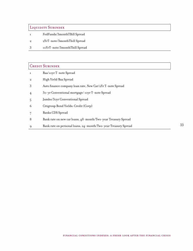
33


Liquidity Subindex

1 FedFunds/3monthTBill Spread



Credit Subindex

1 Baa/10yr T-note Spread

2 High Yield/Baa Spread

3 Auto finance company loan rate, New Car/2Yr T-note Spread

4 30-yr Conventional mortgage/ 10yr T-note Spread

5 Jumbo/30yr Conventional Spread

6 Citigroup Bond Yields: Credit {Corp}

7 Banks CDS Spread

8 Bank rate on new car loans, 48-month/Two-year Treasury Spread

9 Bank rate on personal loans, 24-month/Two-year Treasury Spread

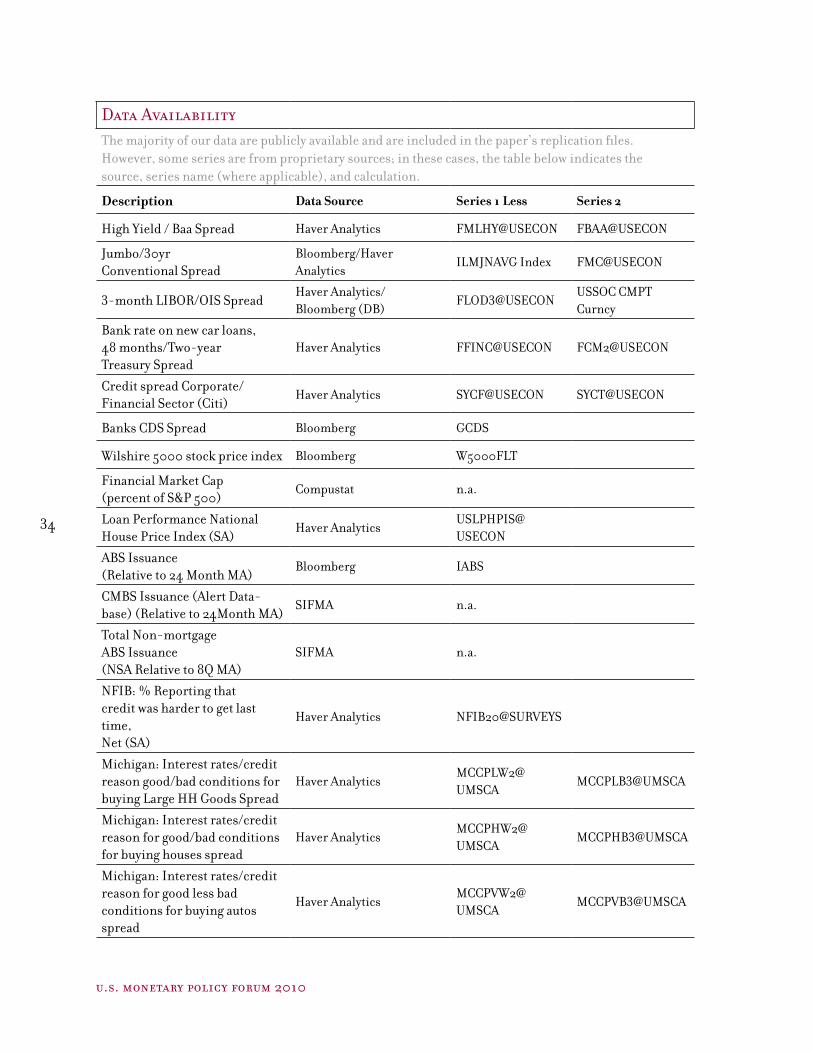
34


Data AvailabilityThe majority of our data are publicly available and are included in the paper’s replication files. However, some series are from proprietary sources; in these cases, the table below indicates the source, series name (where applicable), and calculation.

Description Data Source Series 1 Less Series 2

High Yield / Baa Spread Haver Analytics FMLHY@USECON FBAA@USECON

Jumbo/30yr Conventional Spread

Bloomberg/Haver Analytics

ILMJNAVG Index FMC@USECON

3-month LIBOR/OIS SpreadHaver Analytics/ Bloomberg (DB)

FLOD3@USECONUSSOC CMPT Curncy

Bank rate on new car loans, 48 months/Two-year Treasury Spread

Haver Analytics FFINC@USECON FCM2@USECON

Credit spread Corporate/ Financial Sector (Citi)

Haver Analytics SYCF@USECON SYCT@USECON

Banks CDS Spread Bloomberg GCDS

Wilshire 5000 stock price index Bloomberg W5000FLT

Financial Market Cap (percent of S&P 500)

Compustat n.a.

Loan Performance National House Price Index (SA)

Haver AnalyticsUSLPHPIS@USECON

ABS Issuance (Relative to 24 Month MA)

Bloomberg IABS

CMBS Issuance (Alert Data-base) (Relative to 24Month MA)

SIFMA n.a.

Total Non-mortgage ABS Issuance (NSA Relative to 8Q MA)

SIFMA n.a.

NFIB: % Reporting that credit was harder to get last time, Net (SA)

Haver Analytics NFIB20@SURVEYS

Michigan: Interest rates/credit reason good/bad conditions for buying Large HH Goods Spread

Haver AnalyticsMCCPLW2@UMSCA

MCCPLB3@UMSCA

Michigan: Interest rates/credit reason for good/bad conditions for buying houses spread

Haver AnalyticsMCCPHW2@UMSCA

MCCPHB3@UMSCA

Michigan: Interest rates/credit reason for good less bad conditions for buying autos spread

Haver AnalyticsMCCPVW2@UMSCA

MCCPVB3@UMSCA

35


figure 2.1 a stylized view of financial conditions and the transmission mechanism

financialconditions

policy otherfactors

inflation and

ouptut

36


Table 2.1: Financial Condition Index VariablesVariable Bloomberg Citi

DeutscheBank

Goldman Sachs

KC FedMacro

AdvisersOECD

Yield Spreads

3m LIBOR/3m Treasury (TED) spread X X

2yr swap rate/2yr Treasury spread X

10yr swap rate X

10yr credit default swap spread X

Off-the-run/on-the-run 10yrTreasury spread X

10yr Treasury/Federal funds effective rate spread X

Aaa/10yr Treasury spread X

Baa/10yr Treasury spread X X

Baa/Aaa spread X

High-yield bond/Baa spread X

Consumer ABS /5yr Treasury spread X

Commercial paper/3mTreasury bill spread X

LIBOR/OIS spread X

Muni/10yr Treasury spread X

High yield/10yr Treasury spread X X X

Agency/Treasury spread X

Swaps/Treasury spread X

30yr conventional mortgage rate/10yr Treasury spread X

Investment-grade options-adjusted credit spread X

Interest rates

Federal funds rate X X

10yr Treasury yield X(1)

3m LIBOR X

3m euro-dollar rate X

Aaa corporate bond yield X

Effective mortgage rate X(1)

Behavior of Asset Prices

Correlation between stock & Treasury returns X

Implied volatility of stock prices (VI X index) X X

Idiosyncratic volatility of bank stock prices X

Cross-section dispersion of bank stock returns X

S&P 500 index X X X

Wilshire 5000 index X(1)

Stock market capitalization/GDP X

Dividend/price ratio (S&P 500) X

Median existing 1-family home price X

Trade-weighted dollar X(1) X X X X (1)

Other

Bank lending standards for medium and small firms X

Household equity wealth X

Zero-maturity money stock X(1)

CPI energy price index X(1)

Note: (1) Adjusted for inflation using various inflation measures; Unless indicated, variables are in nominal terms.

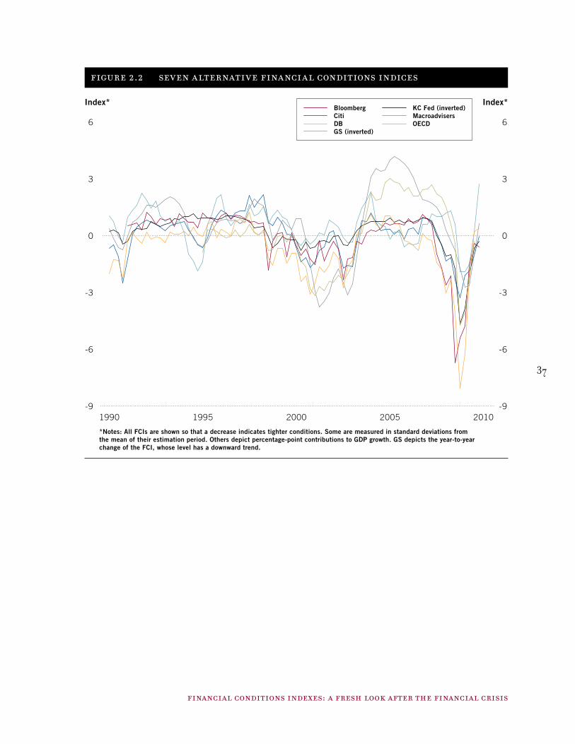
37


figure 2.2 seven alternative financial conditions indices

Index*

*Notes: All FCIs are shown so that a decrease indicates tighter conditions. Some are measured in standard deviations from the mean of their estimation period. Others depict percentage-point contributions to GDP growth. GS depicts the year-to-year change of the FCI, whose level has a downward trend.

Index*

1990 1995 2000 2005 2010

BloombergCitiDBGS (inverted)

KC Fed (inverted)MacroadvisersOECD

-9

-6

-3

0

3

6

-9

-6

-3

0

3

6

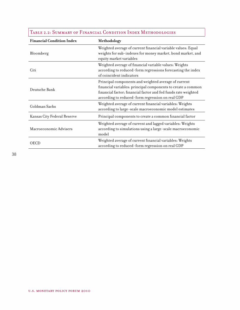
38


Table 2.2: Summary of Financial Condition Index Methodologies

Financial Condition Index Methodology

BloombergWeighted average of current financial variable values: Equal weights for sub-indexes for money market, bond market, and equity market variables

CitiWeighted average of financial variable values: Weights according to reduced-form regressions forecasting the index of coincident indicators

Deutsche Bank

Principal components and weighted average of current financial variables: principal components to create a common financial factor; financial factor and fed funds rate weighted according to reduced-form regression on real GDP

Goldman SachsWeighted average of current financial variables: Weights according to large-scale macroeconomic model estimates

Kansas City Federal Reserve Principal components to create a common financial factor

Macroeconomic AdvisersWeighted average of current and lagged variables: Weights according to simulations using a large-scale macroeconomic model

OECDWeighted average of current financial variables: Weights according to reduced-form regression on real GDP

39


Table 3.1: Results from In-Sample Regressions 1961:1 – 2006:iv

yt+h

– yt = β

0 + ∑ φ

i Δ y

t+1– i + ∑ γ

i x

t+1– i + e

t+i

4

i=1

4

i=1

(a) h = 2Real GDP IP Employment Unemployment Rate

Financial

IndicatorR2

x/∆yF QLR R2

x/∆yF QLR R2

x/∆yF QLR R2

x/∆yF QLR

FedFunds 0.2011.38

(0.000)6.12

(0.002)0.14

8.36 (0.000)

3.00 (0.212)

0.077.65

(0.000)3.75

(0.078)0.11

5.08 (0.000)

5.23 (0.008)

Term Spread 0.084.08

(0.003)9.03

(0.000)0.05

2.85 (0.022)

8.21 (0.000)

0.033.75

(0.005)7.36

(0.000)0.12

5.50 (0.000)

4.48 (0.026)

Credit Spread 0.2014.71

(0.000)10.71

(0.000)0.26

14.92 (0.000)

10.72 (0.000)

0.1110.61

(0.000)10.75

(0.000)0.24

9.79 (0.000)

12.37 (0.000)

Real M2 0.188.75

(0.000)6.38

(0.001)0.17

6.94 (0.000)

4.64 (0.021)

0.065.06

(0.000)5.99

(0.002)0.08

3.26 (0.011)

2.08 (0.567)

SP500 0.096.72

(0.000)5.83

(0.003)0.16

5.55 (0.000)

3.81 (0.072)

0.096.47

(0.000)5.50

(0.005)0.15

5.83 (0.000)

2.57 (0.350)

(b) h = 4Real GDP IP Employment Unemployment Rate

Financial

IndicatorR2

x/∆yF QLR R2

x/∆yF QLR R2

x/∆yF QLR R2

x/∆yF QLR

FedFunds 0.2610.74

(0.000)6.38

(0.001)0.27

10.27 (0.000)

4.87 (0.014)

0.159.17

(0.000)5.15

(0.009)0.26

8.66 (0.000)

8.41 (0.000)

Term Spread 0.132.82

(0.024)10.81

(0.000)0.10

2.64 (0.032)

11.01 (0.000)

0.083.32

(0.010)12.73

(0.000)0.26

5.48 (0.000)

9.13 (0.000)

Credit Spread 0.1210.17

(0.000)11.56

(0.000)0.21

12.21 (0.000)

21.85 (0.000)

0.118.28

(0.000)16.41

(0.000)0.24

10.27 (0.000)

19.56 (0.000)

Real M2 0.237.78

(0.000)9.96

(0.000)0.23

6.76 (0.000)

6.05 (0.002)

0.104.63

(0.001)8.53

(0.000)0.15

2.84 (0.023)

2.64 (0.326)

SP500 0.073.97

(0.003)2.72

(0.297)0.16

5.78 (0.000)

3.42 (0.123)

0.105.09

(0.000)4.56

(0.023)0.17

4.57 (0.001)

3.02 (0.207)

Notes: R2 x/∆y

denotes the partial R2 for the lags of x conditional on the lags if Δy. F denotes the F-statistic associated with the null hypothesis that all of the γ

i coefficients are equal to zero, where the p-value is

shown in parentheses. QLR is the “sup-Chow” F-statistic testing for stability of the γi coefficients

(p-value in parentheses). These test statistics using HAC covariance estimators with 2 lags for h = 2 and 8 lags for h = 4.

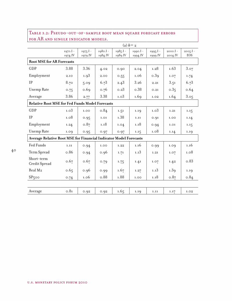
40


Table 3.2: Pseudo-out-of-sample root mean square forecast errorsfor AR and single indicator models.

(a) h = 21970.I - 1974.IV

1975.I - 1979.IV

1980.I - 1984.IV

1985.I - 1989.IV

1990.I - 1994.IV

1995.I - 1999.IV

2000.I - 2004.IV

2005.I - EOS

Root MSE for AR Forecasts

GDP 3.88 3.36 4.02 0.90 2.04 1.28 1.63 3.07

Employment 2.10 1.93 2.00 0.55 1.06 0.39 1.07 1.74

IP 8.70 5.09 6.73 2.43 3.26 2.21 3.51 6.73

Unemp Rate 0.75 0.69 0.76 0.23 0.38 0.21 0.35 0.64

Average 3.86 2.77 3.38 1.03 1.69 1.02 1.64 3.05

Relative Root MSE for Fed Funds Model Forecasts

GDP 1.03 1.00 0.84 1.51 1.19 1.03 1.21 1.15

IP 1.08 0.95 1.01 1.38 1.11 0.91 1.00 1.14

Employment 1.24 0.87 1.18 1.04 1.18 0.94 1.01 1.15

Unemp Rate 1.09 0.95 0.97 0.97 1.15 1.08 1.14 1.19

Average Relative Root MSE for Financial Indicator Model Forecasts

Fed Funds 1.11 0.94 1.00 1.22 1.16 0.99 1.09 1.16

Term Spread 0.86 0.94 0.96 1.71 1.13 1.21 1.07 1.08

Short-term Credit Spread

0.67 0.67 0.79 1.75 1.41 1.07 1.42 0.83

Real M2 0.65 0.96 0.99 1.67 1.27 1.13 1.39 1.19

SP500 0.74 1.06 0.88 1.88 1.00 1.18 0.87 0.84

Average 0.81 0.92 0.92 1.65 1.19 1.11 1.17 1.02

41


(b) h = 41970.I - 1974.IV

1975.I - 1979.IV

1980.I - 1984.IV

1985.I - 1989.IV

1990.I - 1994.IV

1995.I - 1999.IV

2000.I - 2004.IV

2005.I - EOS

Root MSE for AR Forecasts

GDP 3.55 2.46 3.33 0.99 1.75 1.01 1.41 3.17

Employment 2.13 1.78 2.20 0.65 1.33 0.38 1.46 2.52

IP 8.19 4.13 5.64 2.33 2.50 2.16 3.54 6.87

Unemp Rate 1.58 1.08 1.56 0.51 0.75 0.32 0.69 1.63

Average 3.86 2.36 3.18 1.12 1.58 0.97 1.78 3.55

Average Relative Root MSE for Financial Indicator Model Forecasts

Fed Funds 0.84 1.02 0.84 1.36 1.25 1.06 1.12 1.15

Term Spread 0.75 0.87 0.90 1.98 1.26 1.40 1.09 1.05

Short-term Credit Spread

0.71 0.78 0.80 1.43 1.33 0.90 1.40 0.89

Real M2 0.47 0.95 0.89 1.63 1.38 1.19 1.43 1.14

SP500 0.76 1.14 0.89 1.73 1.00 1.04 0.87 0.89

Average 0.71 0.95 0.86 1.63 1.24 1.12 1.18 1.02

Notes: The top panels of the tables show the root mean square forecast errors (RMSE) for the AR models over the indicated sample periods for the real activity variable listed in the first column of the table. The bottom panels shows the corresponding RMSE of the forecasts based on the financial indicators relative to the AR forecasts. The four entries for each financial indicator correspond to the four real activity variables (GDP, IP, Employment, Unemployment Rate). The last rows the table shows the average relative RMSE across the real activity and financial indicators.

42


Table 3.3: Average Relative RMSE for Various FCI forecasting models(a) h = 2

FCI 1970.I - 1974.IV

1975.I - 1979.IV

1980.I - 1984.IV

1985.I - 1989.IV

1990.I - 1994.IV

1995.I - 1999.IV

2000.I - 2004.IV

2005.I - EOS

BLOOMBERG 0.94 0.92

CITI 0.93 0.78 0.88

DB (PC) 0.91 0.91

DB (FCI) 0.90 0.87

GS 1.26 1.02 0.84 0.94

KCFSI 0.95 1.00

MA 1.17 0.96 0.95

OECD 1.11

Average all FCIs 1.26 1.04 0.90 0.95

Average from Table 3.2

0.81 0.92 0.92 1.65 1.19 1.11 1.17 1.02

(b) h = 4

FCI 1970.I - 1974.IV

1975.I - 1979.IV

1980.I - 1984.IV

1985.I - 1989.IV

1990.I - 1994.IV

1995.I - 1999.IV

2000.I - 2004.IV

2005.I - EOS

BLOOMBERG 1.41 0.80

CITI 1.02 0.75 0.83

DB (PC) 1.15 0.78

DB (FCI) 1.18 0.78

GS 1.28 1.03 0.81 0.91

KCFSI 0.81 0.84

MA 1.29 0.92 0.83

OECD 0.90

Average all FCIs 1.28 1.12 1.00 0.83

Average from Table 3.2

0.71 0.95 0.86 1.63 1.24 1.12 1.18 1.02

Notes: GS refers to the Goldman Sachs FCI in first difference. DB (PC) and DB (FCI) refer to the Deustche Bank principal component and FCI. See Table 3.2 for additional notes.

43


Tabl

e 4.

1: F

inan

cial

Ind

icat

ors

Des

crip

tion

NU

TSo

urce

Star

tEn

dR

2 – N

umbe

r of F

acto

rsΛ

1

Inte

rest

Rat

es0

12

34

110

-Yea

r Tre

asur

y N

ote

Yiel

d at

Con

stan

t Mat

urit

y2

Fede

ral R

eser

ve B

oard

1970

:2

2009

:4

0.15

0.

32

0.40

0.

430.

46-0

.36

2Fe

dFun

ds/3

mon

thTB

ill S

prea

dX

1 Fe

dera

l Res

erve

Boa

rd19

70:2

20

09:4

0.

42

0.62

0.

62

0.68

0.68

-0.4

3

32Y

rT-n

ote/

3mon

thTb

ill S

prea

dX

1 Fe

dera

l Res

erve

Boa

rd19

76:3

20

09:4

0.

03

0.27

0.

34

0.48

0.76

0.2

5

410

YrT-

note

/3m

onth

Tbill

Spr

ead

X1

Fede

ral R

eser

ve B

oard

1970

:2

2009

:4

0.21

0.

39

0.57

0.

750.

77 0

.38

5Ba

a/10

yr T

-not

e Sp

read

1 Fe

dera

l Res

erve

Boa

rd19

70:2

20

09:4

0.

39

0.44

0.

82

0.82

0.83

-0.0

6

6H

igh

Yiel

d / B

aa S

prea

d1

Mer

rill

Lync

h/

Fede

ral R

eser

ve B

oard

1997

:1

2009

:4

0.73

0.

92

0.95

0.

950.

95-0

.17

7A

uto

fina

nce

com

pany

loan

rate

, new

Car

/ Tw

o-yr

Tre

asur

y Sp

read

X1

Fede

ral R

eser

ve B

oard

1976

:3

2009

:4

0.06

0.

40

0.41

0.

710.

730.

46

830

-yr C

onve

ntio

nal m

ortg

age/

10yr

TBon

d Sp

read

1 Fe

dera

l Res

erve

Boa

rd19

71:2

20

09:4

0.

23

0.34

0.

42

0.54

0.66

-0.2

3

9Ju

mbo

/30y

r Con

vent

iona

l Spr

ead

X1

Deu

tsch

e Ba

nk19

98:3

20

09:4

0.

60

0.94

0.

94

0.96

0.96

-0.4

4

10TE

D S

prea

d (U

sing

Con

stan

t Mat

urit

y T-

bill)

1 Fe

dera

l Res

erve

Boa

rd19

81:4

20

09:4

0.

32

0.72

0.

76

0.75

0.84

-0.6

1

113-

mon

th L

IBO

R/O

IS1

Bloo

mbe

rg/F

eder

al R

eser

ve B

oard

2002

:1

2009

:4

0.71

0.

97

0.97

0.

970.

98-0

.35

12Ba

nk ra

te o

n ne

w C

ar L

oans

, 48-

mon

th/

Two-

year

Tre

asur

y Sp

read

X1

Wal

l Str

eet J

ourn

al/

Fede

ral R

eser

ve B

oard

1976

:3

2009

:4

0.37

0.

59

0.81

0.

800.

870.

37

13Ba

nk ra

te o

n Pe

rson

al L

oans

, 24-

mon

th/

Two-

year

Tre

asur

y Sp

read

X1

Fede

ral R

eser

ve B

oard

1976

:3

2009

:4

0.72

0.

81

0.85

0.

840.

930.

22

14Ci

tigr

oup

Bond

Yie

lds:

Cred

it {C

orp}

Spr

ead/

Fina

nce

X1

Citi

1980

:1

2009

:4

0.28

0.

73

0.75

0.

730.

78-0

.65

15Ba

nks

CDS

Spre

adX

1 D

euts

che

Bank

2004

:4

2009

:4

0.88

0.

99

0.99

0.

990.

99-0

.10

Pric

es

16R

eal B

road

Tra

de-W

eigh

ted

Exch

ange

Val

ue o

f the

US$

5

Fede

ral R

eser

ve B

oard

1973

:2

2009

:4

0.02

0.

19

0.20

0.

210.

29-0

.24

17W

ilshi

re 5

000

5 W

ilshi

re A

ssoc

iate

s19

71:2

20

09:4

0.

09

0.36

0.

46

0.46

0.49

0.48

18Fi

nanc

ial M

arke

t Cap

(per

cent

of S

&P

500)

X5

Stan

dard

and

Poo

r’s

1976

:4

2009

:4

0.04

0.

34

0.41

0.

410.

400.

38

19Lo

an P

erfo

rman

ce N

atio

nal H

ouse

Pri

ce In

dex

(SA

)X

5 Fi

rstA

mer

ican

Cor

e Lo

gic

1976

:2

2009

:4

0.31

0.

57

0.60

0.

660.

690.

43

20Pr

ice

of O

il R

elat

ive

to 2

Year

MA

(PPI

Cru

de O

il)X

4 W

all S

tree

t Jou

rnal

1970

:2

2009

:4

0.13

0.

18

0.28

0.

300.

26-0

.18

Qua

ntit

ies

21Ba

nk C

redi

t: A

ll Co

mm

erci

al B

anks

(SA

)X

5 Fe

dera

l Res

erve

Boa

rd19

70:2

20

09:4

0.

28

0.32

0.

33

0.53

0.59

0.02

22Co

mm

erci

al P

aper

Out

stan

ding

:All

Issu

ers

(SA

)X

5 Fe

dera

l Res

erve

Boa

rd19

70:2

20

09:4

0.

32

0.39

0.

52

0.58

0.71

-0.1

7

23Co

mm

erci

al P

aper

Issu

ance

(Rel

ativ

e to

24M

onth

MA

)1

Fede

ral R

eser

ve B

oard

2002

:1

2009

:4

0.79

0.

97

0.98

0.

980.

99-0

.14

44


Des

crip

tion

NU

TSo

urce

Star

tEn

dR

2 – N

umbe

r of F

acto

rsΛ

1

Qua

ntit

ies,

cont

.0

12

34

24A

BS Is

suan

ce (R

elat

ive

to 2

4Mon

th M

A)

1 Bl

oom

berg

1997

:1

2009

:4

0.32

0.

92

0.92

0

.93

0.9

6 0

.68

25CM

BS Is

suan

ce (A

lert

Dat

abas

e) (R

elat

ive

to 2

4Mon

th M

A)

1D

euts

che

Bank

1992

:1

2009

:4

0.29

0.

79

0.79

0

.82

0.9

0 0

.51

26M

oney

Sto

ck:M

ZM {Z

ero

Mat

urit

y} (S

A)

5 Fe

dera

l Res

erve

Ban

k of

St.

Loui

s19

74:2

20

09:4

0.

13

0.30

0.

49

0.5

5 0

.52

0.2

1

27St

ate

& lo

cal G

over

nmen

t:Lia

bilit

y:

Cred

it M

arke

t Ins

trum

ents

(SA

)X

5 Fe

dera

l Res

erve

Boa

rd19

70:2

20

09:4

0.

04

0.13

0.

22

0.5

4 0

.55

0.2

1

28N

onfe

dera

l Sec

tors

:Lia

bilit

y:

Cred

it M

arke

t Deb

t Out

stan

ding

(SA

)X

5 Fe

dera

l Res

erve

Boa

rd19

70:2

20

09:4

0.

47

0.50

0.

50

0.8

8 0

.88

0.0

6

29Pr

ivat

e N

onfi

nanc

ial D

ebt,

SAX

5 Fe

dera

l Res

erve

Boa

rd19

70:2

20

09:4

0.

52

0.54

0.

55

0.8

5 0

.85

0.0

2

30To

tal F

inan

ce:L

iabi

litie

s:Se

curi

ty R

Ps (N

SA)

X5

Fede

ral R

eser

ve B

oard

1974

:2

2009

:4

0.07

0.

31

0.42

0

.43

0.5

0 0

.36

31A

BS Is

suer

s:A

sset

s; C

onsu

mer

Cre

dit (

NSA

) X

5 Fe

dera

l Res

erve

Boa

rd19

92:2

20

09:3

0.

16

0.67

0.

73

0.7

5 0

.85

0.3

0

32A

BS Is

suer

s:A

sset

; Mor

tgag

es o

n 1-

4 Fa

mily

Str

uctu

res

(NSA

) X

5 Fe

dera

l Res

erve

Boa

rd19

88:2

20

09:4

0.

22

0.73

0.

76

0.7

6 0

.88

0.6

2

33A

BS Is

suer

s:A

sset

; Com

mer

cial

Mor

tgag

es (N

SA)

X5

Fede

ral R

eser

ve B

oard

1993

:2

2009

:4

0.28

0.

75

0.75

0

.81

0.9

2 0

.34

34To

tal N

on-m

ortg

age

ABS

Issu

ance

(NSA

) Rel

ativ

e to

8Q

MA

)1

Deu

tsch

e Ba

nk19

94:1

20

09:4

0.

28

0.90

0.

90

0.8

9 0

.94

0.7

8

35Br

oker

Dea

ler L

ever

age

X5

Fede

ral R

eser

ve B

oard

1970

:2

2009

:4

0.03

0.

14

0.20

0

.19

0.2

3 0

.24

Surv

eys

36N

FIB:

%R

epor

ting

that

Cre

dit

Was

Har

der t

o G

et L

ast T

ime,

Net

(SA

)X

1N

atio

nal F

eder

atio

n of

In

depe

nden

t Bus

ines

s19

86:1

20

09:4

0.

42

0.69

0.

69

0.8

4 0

.84

-0.2

2

37M

ichi

gan

Surv

ey:I

nter

est R

ates

/Cre

dit R

easo

n G

ood/

Bad

Cond

itio

ns fo

r Buy

ing

Larg

e H

H G

oods

Spr

ead

X1

Uni

vers

ity

of M

ichi

gan

1978

:1

2009

:4

0.68

0.

81

0.82

0

.83

0.9

1 -0

.29

38M

ichi

gan

Surv

ey:I

nter

est R

ates

/Cre

dit R

easo

n fo

r Goo

d/Ba

d Co

ndit

ions

for B

uyin

g H

ouse

s Sp

read

X1

Uni

vers

ity

of M

ichi

gan

1980

:2

2009

:4

0.70

0.

86

0.87

0

.86

0.9

3 -0

.35

39M

ichi

gan

Surv

ey:I

nter

est R

ates

/Cre

dit R

easo

n fo

r Goo

d Le

ss

Bad

Cond

itio

ns fo

r Buy

ing

Aut

os S

prea

dX

1U

nive

rsit

y of

Mic

higa

n19

78:1

20

09:4

0.

56

0.75

0.

80

0.8

2 0

.89

-0.3

6

40FR

B Sr

. Of.

Ban

ks T

ight

enin

g C&

I Loa

ns to

Lar

ge F

irm

s (%

)X

1U

nive

rsit

y of

Mic

higa

n19

90:2

20

09:4

0.

45

0.81

0.

83

0.8

3 0

.88

-0.4

5

41FR

B Sr

. Of.

:Ban

ks T

ight

enin

g C&

I Loa

ns to

Sm

all F

irm

s (%

)X

1U

nive

rsit

y of

Mic

higa

n19

90:2

20

09:4

0.

54

0.86

0.

87

0.8

7 0

.91

-0.4

8

42FR

B Sr

. Of.

:Ban

ks W

illin

gnes

s to

Len

d to

Con

sum

ers

(%)

X1

Uni

vers

ity

of M

ichi

gan

1970

:2

2009

:4

0.24

0.

59

0.60

0

.63

0.6

6 0

.58

2nd

Mom

ents

43Co

rrel

atio

n of

Ret

urns

on

Equi

ties

and

Tre

asur

ies

1 A

utho

rs’ c

alcu

lati

ons

base

d on

St

anda

rd a

nd P

oor’

s an

d

US

Trea

sury

dat

a19

76:3

20

09:4

0.

18

0.38

0.

47

0.5

1 0

.69

0.2

3

44Id

iosy

ncra

tic

Bank

Sto

ck V

olat

ility

1 G

oldm

an S

achs

1973

:1

2009

:4

0.20

0.

52

0.71

0

.72

0.7

7 -0

.53

45M

onth

ly A

vera

ge V

IX

1 Ch

icag

o O

ptio

ns E

xcha

nge

1986

:1

2009

:4

0.24

0.

73

0.81

0

.8

0.8

2 -0

.64

Ave

rage

R2

0.29

0.41

0.49

0.57

0.65

45


Notes for Table 4.1: In the column labeled NU, an “X” denotes variable was not used in any of the alternative FCIs we have surveyed. The column labeled T shows the transformation (1=level, 2=first difference, 4 = logarithm, 5 = first difference of logarithm). The start and end dates indicate the periods the series was used in to estimate the factors. The five columns labeled R2 show the R2 for model including A(L)Y, and then sequentially adding 0, 1, and 4 factors. The column labeled Λ

1 shows the

estimated value of Λ for the single factor model.

figure 4.1 number of financial indicators by date

No. of Indicators No. of Indicators

1970 1975 1980 1985 1990 1995 2000 2005 20100

5

10

15

20

25

30

35

40

45

0

5

10

15

20

25

30

35

40

45

46


figure 4.2 ranking of variables by their lambdas in single factor model

0.0 0.1 0.2 0.3 0.4 0.5 0.6 0.7 0.8

34. Total Non-mortgage ABS Issuance (0.78)24. ABS Issuance (0.68)

14. Citigroup Bond Yields:Credit {Corp} Spread (0.65)45. Monthly Average VIX (0.64)

32. ABS Issuers:Asset: Home Mtgs. (0.62)10. TED Spread (Constant Maturity T-bill) (0.61)

42. FRB: Banks Willingness to Lend to Cons. (0.58)44. Idiosyncratic Bank Stock Volatility (0.53)25. CMBS Issuance (Alert Database) (0.51)

41. FRB: Banks Tight. C&I Loans to Small Firms (0.48)17. Wilshire 5000 (0.48)

7. Auto fin company loan rate, new Car Treas Spread (0.46)40. FRB: Banks Tight. C&I Loans to Large Firms (0.45)

9. Jumbo/30yr Conventional Spread (0.44)19. Loan Performance National House Price Index (0.43)

2. FedFunds/3monthTBill Spread (0.43)18. Financial Market Cap (percent of S&P 500) (0.38)

4. 10-YrT-note/3monthTbill Spread (0.38)12. Bank Rate: New Car Loans, Treas Spread (0.37)

39. U. Mich: Buying Conds. Autos (0.36)30. Total Finance:Liabilities:Security RPs (0.36)

1. 10-Yr Treas Note Yld at Constant Maturity (0.36)38. U. Mich: Buying Conditions Houses (0.35)

11. 3-m LIBOR/OIS (0.35)33. ABS Issuers: Asset; Comm. Mtgs. (0.34)

31. ABS Issuers: Assets; Cons. Credit (0.3)37. U. Mich: Buying Conditions Large HH Goods (0.29)

3. 2Yr T-note/3m Tbill Spread (0.25)35. Broker Dealer Leverage (0.24)

16. Real Broad TW Exchange Value of the US$ (0.24)43. Correl of Returns on Equities and Treas (0.23)

8. 30-yr Conv. mtg/ 10-yrTBond Spread (0.23)36. NFIB: %Reporting Credit Harder to Get (0.22)

13. Bank Rate on Personal Loans, Treas Spread (0.22)27. S&L Govt: Liability: Credit Market Instruments (0.21)

26. Money Stock: MZM (0.21)20. Price of Oil (PPI Crude Oil) (0.18)

22. Comm. Paper Outst: All Issuers (0.17)6. High Yld / Baa Spread (0.17)

23. Comm. Paper Issuance (0.14)15. Banks CDS Spread (0.1)

28. Nonfed Sectors: Credit Market Debt Outst. (0.06)5. Baa/10yr T-note Spread (0.06)

29. Private Nonfinancial Debt (0.02)21. Bank Credit: All Commercial Banks (0.02)

Financial Indicator (lambda absolute value)*

*Numbers preceding variable name correspond to line numbers in Table 4.1.

Absolute value of lambda L1 (ABS)

47


figure 4.3 ranking of variables by their lambdas in single factor model

Financial Indicator (lambda value)*

*Numbers preceding variable name correspond to line numbers in Table 4.1.

Lambda Value (L1)

-0.6 -0.4 -0.2 0.0 0.2 0.4 0.6 0.8

34. Total Non-mortgage ABS Issuance (0.78)24. ABS Issuance (0.68)

32. ABS Issuers:Asset: Home Mtgs. (0.62)42. FRB: Banks Willingness to Lend to Cons. (0.58)

25. CMBS Issuance (Alert Database) (0.51)17. Wilshire 5000 (0.48)

7. Auto fin company loan rate, new Car Treas Spread (0.46)19. Loan Performance National House Price Index (0.43)

18. Financial Market Cap (percent of S&P 500) (0.38)4. 10-YrT-note/3monthTbill Spread (0.38)

12. Bank Rate: New Car Loans, Treas Spread (0.37)30. Total Finance:Liabilities:Security RPs (0.36)

33. ABS Issuers: Asset; Comm. Mtgs. (0.34)31. ABS Issuers: Assets; Cons. Credit (0.3)

3. 2Yr T-note/3m Tbill Spread (0.25)35. Broker Dealer Leverage (0.24)

43. Correl of Returns on Equities and Treas (0.23)13. Bank Rate on Personal Loans, Treas Spread (0.22)

27. S&L Govt: Liability: Credit Market Instruments (0.21)26. Money Stock: MZM (0.21)

28. Nonfed Sectors: Credit Market Debt Outst. (0.06)29. Private Nonfinancial Debt (0.02)

21. Bank Credit: All Commercial Banks (0.02)5. Baa/10yr T-note Spread (-0.06)

15. Banks CDS Spread (-0.1)23. Comm. Paper Issuance (-0.14)

22. Comm. Paper Outst: All Issuers (-0.17)6. High Yld / Baa Spread (-0.17)

20. Price of Oil (PPI Crude Oil) (-0.18)36. NFIB: %Reporting Credit Harder to Get(-0.22)

8. 30-yr Conv. mtg/ 10-yrTBond Spread (-0.23)16. Real Broad TW Exchange Value of the US$ (-0.24)

37. U. Mich: Buying Conditions Large HH Goods (-0.29)38. U. Mich: Buying Conditions Houses (-0.35)

11. 3-m LIBOR/OIS (-0.35)39. U. Mich: Buying Conds. Autos (-0.36)

1. 10-Yr Treas Note Yld at Constant Maturity (-0.36)2. FedFunds/3monthTBill Spread (-0.43)

9. Jumbo/30yr Conventional Spread (-0.44)40. FRB: Banks Tight. C&I Loans to Large Firms (-0.45)41. FRB: Banks Tight. C&I Loans to Small Firms (-0.48)

44. Idiosyncratic Bank Stock Volatility (-0.53)10. TED Spread (Constant Maturity T-bill) (-0.61)

45. Monthly Average VIX (-0.64)14. Citigroup Bond Yields:Credit {Corp} Spread (-0.65)

48


figure 5.1 new fci: first principal component of 45 financial indicators

Index* Index*

1970 1975 1980 1985 1990 1995 2000 2005 2010-3

-2

-1

0

1

2

3

4

-3

-2

-1

0

1

2

3

4

*Index measured in terms of number of standard deviations away from historical mean.

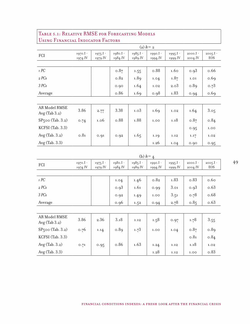
49


Table 5.1: Relative RMSE for Forecasting Models Using Financial Indicator Factors

(a) h = 2

FCI 1970.I - 1974.IV

1975.I - 1979.IV

1980.I - 1984.IV

1985.I - 1989.IV

1990.I - 1994.IV

1995.I - 1999.IV

2000.I - 2004.IV

2005.I - EOS

1 PC 0.87 1.55 0.88 1.60 0.93 0.66

2 PCs 0.82 1.89 1.04 1.87 1.01 0.69

3 PCs 0.90 1.64 1.02 2.03 0.89 0.73

Average 0.86 1.69 0.98 1.83 0.94 0.69

AR Model RMSE Avg (Tab 3.2)

3.86 2.77 3.38 1.03 1.69 1.02 1.64 3.05

SP500 (Tab. 3.2) 0.74 1.06 0.88 1.88 1.00 1.18 0.87 0.84

KCFSI (Tab. 3.3) 0.95 1.00

Avg (Tab. 3.2) 0.81 0.91 0.92 1.65 1.19 1.12 1.17 1.02

Avg (Tab. 3.3) 1.26 1.04 0.90 0.95

(b) h = 4

FCI 1970.I - 1974.IV

1975.I - 1979.IV

1980.I - 1984.IV

1985.I - 1989.IV

1990.I - 1994.IV

1995.I - 1999.IV

2000.I - 2004.IV

2005.I - EOS

1 PC 1.04 1.46 0.82 1.83 0.83 0.60

2 PCs 0.93 1.61 0.99 3.01 0.93 0.63

3 PCs 0.92 1.49 1.00 3.51 0.78 0.68

Average 0.96 1.52 0.94 2.78 0.85 0.63

AR Model RMSE Avg (Tab 3.2)

3.86 2.36 3.18 1.12 1.58 0.97 1.78 3.55

SP500 (Tab. 3.2) 0.76 1.14 0.89 1.73 1.00 1.04 0.87 0.89

KCFSI (Tab. 3.3) 0.81 0.84

Avg (Tab. 3.2) 0.71 0.95 0.86 1.63 1.24 1.12 1.18 1.02

Avg (Tab. 3.3) 1.28 1.12 1.00 0.83

50


figure 5.2 real gdp growth: forecast using autoregressive and new fci models (h=2)*

Q/Q% AR

*2 quarters horizon

Q/Q% AR

1970 1975 1980 1985 1990 1995 2000 2005 2010-8

-6

-4

-2

0

2

4

6

8

10

-8

-6

-4

-2

0

2

4

6

8

10

ActualAutoregressiveNew FCI

figure 5.3a real gdp growth: forecast using sp500 and new fci (h=2)*

Q/Q% AR

*2 quarters horizon

Q/Q% AR

1990 1995 2000 2005 2010

ActualS&P 500New FCI

-8

-6

-4

-2

0

2

4

6

8

-8

-6

-4

-2

0

2

4

6

8

51


figure 5.3b real gdp growth: forecast using alternative fcis (h=2)*

Q/Q% AR

*2 quarters horizon

Q/Q% AR

1990 1995 2000 2005 2010

ActualCITIDB (PC)

GS (FD)KCSFIMacroadvisers

-8

-6

-4

-2

0

2

4

6

8

-8

-6

-4

-2

0

2

4

6

8

52


Table 5.2: Relative RMSE for Subsets of Financial Indicators(a) h = 2

Subset 1970.I - 1974.IV

1975.I - 1979.IV

1980.I - 1984.IV

1985.I - 1989.IV

1990.I - 1994.IV

1995.I - 1999.IV

2000.I - 2004.IV

2005.I - EOS

New FCI 0.87 1.55 0.88 1.60 0.93 0.66

Balanced Panel 0.82 1.35 0.91 2.20 0.88 0.75

Price 2.29 1.13 1.54 0.82 0.80

Quantity . . . . 1.08

Surveys . . . 1.17 0.91

Liquidity 1.43 0.89 1.81 0.84 0.98

Credit . 1.42 1.11 0.96 0.90

Not purged of either macro influence or fed funds

0.73 1.38 1.08 0.97 1.10 0.86

Purged of both macro influence and fed funds

1.01 1.58 0.95 1.30 0.94 0.74

(b) h = 4

Subset 1970.I - 1974.IV

1975.I - 1979.IV

1980.I - 1984.IV

1985.I - 1989.IV

1990.I - 1994.IV

1995.I - 1999.IV

2000.I - 2004.IV

2005.I - EOS

New FCI 1.08 1.40 0.81 1.93 0.77 0.60

Balanced Panel 0.85 1.22 0.90 3.01 0.73 0.68

Price 0.97 1.04 1.61 0.75 0.72

Quantity . . . . 0.80

Surveys . . . 1.62 0.77

Liquidity 0.85 0.72 2.95 0.75 0.87

Credit . 1.50 1.19 0.92 0.89

Not purged of either macro influence or fed funds

0.89 1.30 1.03 0.84 1.09 0.89

Purged of both macro influence and fed funds

1.21 1.29 0.87 1.22 0.86 0.73

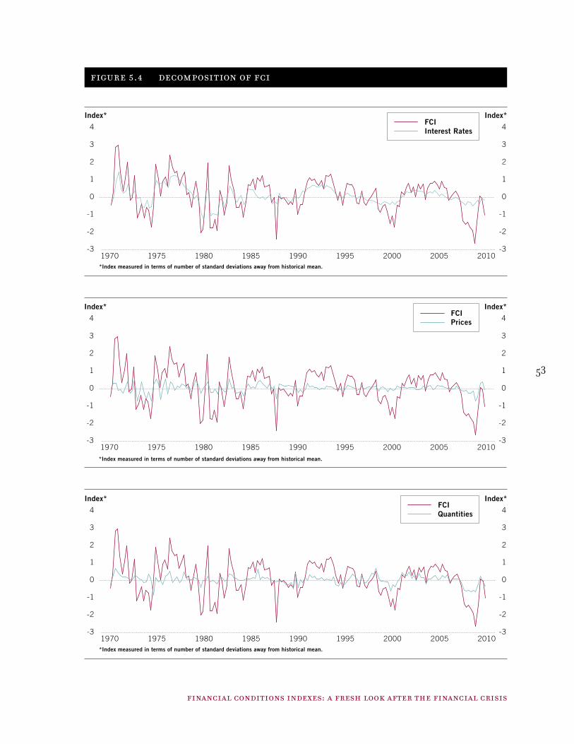
53


figure 5.4 decomposition of fci

Index* Index*

1970 1975 1980 1985 1990 1995 2000 2005 2010-3

-2

-1

0

1

2

3

4

-3

-2

-1

0

1

2

3

4


FCIInterest Rates

Index* Index*

1970 1975 1980 1985 1990 1995 2000 2005 2010-3

-2

-1

0

1

2

3

4

-3

-2

-1

0

1

2

3

4


FCIPrices

Index* Index*

1970 1975 1980 1985 1990 1995 2000 2005 2010-3

-2

-1

0

1

2

3

4

-3

-2

-1

0

1

2

3

4


FCIQuantities

54


figure 5.4 decomposition of fci, cont.

Index* Index*

1970 1975 1980 1985 1990 1995 2000 2005 2010-3

-2

-1

0

1

2

3

4

-3

-2

-1

0

1

2

3

4


FCISurveys

FCI2nd Moments

Index* Index*

1970 1975 1980 1985 1990 1995 2000 2005 2010-3

-2

-1

0

1

2

3

4

-3

-2

-1

0

1

2

3

4


55


figure 5.5 fci with and without purging of business cycle

Index* Index*

1970 1975 1980 1985 1990 1995 2000 2005 2010


-4

-3

-2

-1

0

1

2

3

4

-4

-3

-2

-1

0

1

2

3

4

With A(L)Y adjustmentWithout A(L)Y adjustment

figure 5.6 fci and fci purged of fed fund shocks

Index* Index*

1970 1975 1980 1985 1990 1995 2000 2005 2010


-4

-3

-2

-1

0

1

2

3

4

-4

-3

-2

-1

0

1

2

3

4

BenchmarkAdding Fed Funds to Y

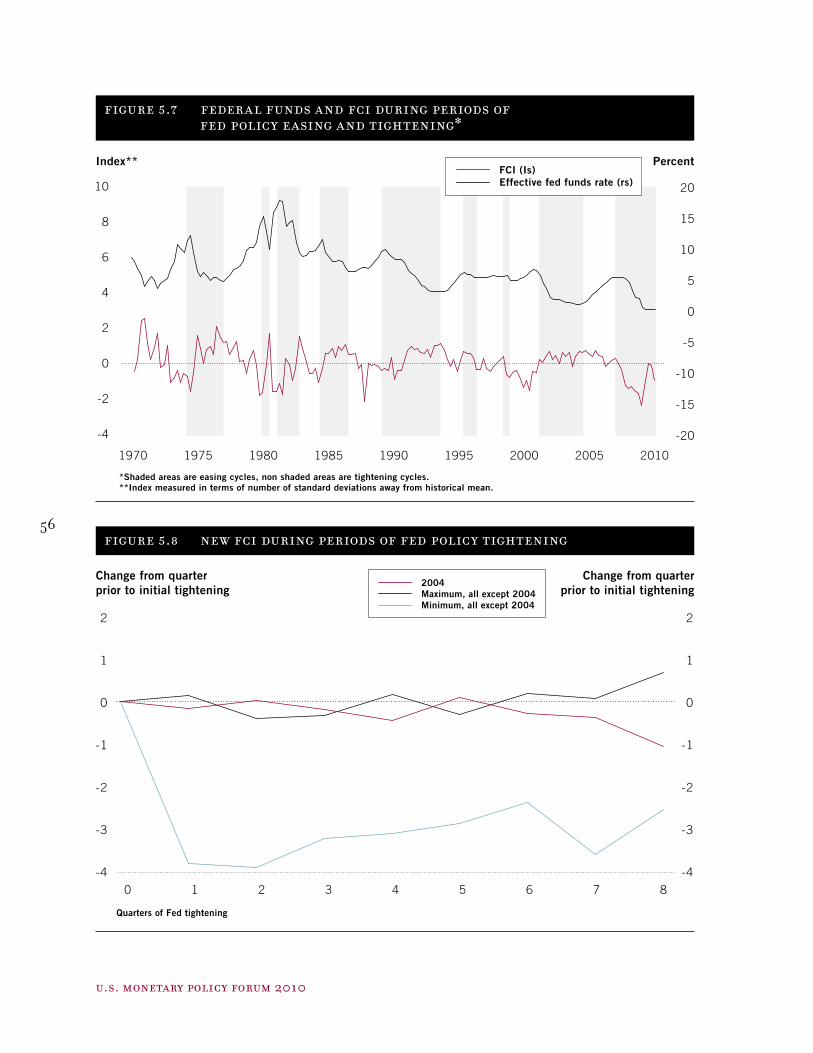
56


figure 5.7 federal funds and fci during periods of fed policy easing and tightening*

Index** Percent

1970 1975 1980 1985 1990 1995 2000 2005 2010

*Shaded areas are easing cycles, non shaded areas are tightening cycles.**Index measured in terms of number of standard deviations away from historical mean.

10

8

6

4

2

0

-2

-4

FCI (Is)Effective fed funds rate (rs)

-20

-15

-10

-5

0

5

10

15

20

figure 5.8 new fci during periods of fed policy tightening

Change from quarter prior to initial tightening

Quarters of Fed tightening

Change from quarterprior to initial tightening

0 1 2 3 4 5 6 7 8

2004Maximum, all except 2004Minimum, all except 2004

-4

-3

-2

-1

0

1

2

-4

-3

-2

-1

0

1

2

57


figure 5.9 new fci during periods of fed policy easing

Change from quarter prior to initial easing

Quarters of Fed easing

Change from quarterprior to initial easing

0 1 2 3 4 5 6 7 8

2007Maximum, all except 2007Minimum, all except 2007

-3

-2

-1

0

1

2

3

4

5

-3

-2

-1

0

1

2

3

4

5

figure 5.10 changes in financial conditions from 2009q2 to 2009 q4

Index* Index*


-1.2

-1.0

-0.8

-0.6

-0.4

-0.2

0.0

0.2

0.4

0.6

-1.2

-1.0

-0.8

-0.6

-0.4

-0.2

0.0

0.2

0.4

0.6

TotalInterestRates

AssetPrices

Quantities Surveys2nd

Moments

UnpurgedPurged

58


Table 5.3: Top contributors to decline in new FCI (2009:Q2 to 2009:Q4)

IndicatorFCI

(purged)FCI

(non purged)Difference

Total Non-mortgage ABS Issuance (Relative to 8Q MA)

-0.20 -0.01 -0.19

Financial Market Cap (percent of S&P 500) -0.19 -0.02 -0.17

ABS Issuers: Assets; Consumer Credit -0.10 -0.03 -0.08

Total Finance: Liabilities - Security RPs -0.10 -0.01 -0.10

Wilshire 5000 -0.10 -0.02 -0.08

ABS Issuers: Asset - Commercial Mortgages -0.09 -0.01 -0.08

FRB SLO: Banks Tightening C&I Loans to Small Firms

-0.08 0.06 -0.14

FRB SLO: Banks Tightening C&I Loans to Large Firms

-0.08 0.05 -0.12

ABS Issuance (Relative to 24M MA) -0.07 0.02 -0.09

Loan Performance National House Price Index -0.07 0.00 -0.07

Sum -1.08 0.02 -1.11

Notes: Columns 2 and 3 show the change from 2009:Q2 to 2009:Q4 in the contribution to the FCI from the indicator shown in column 1.

59


figure 5.11 abs issuance still subdued

$ bln/qtr $ bln/qtr

1993 1995 1997 1999 2001 2003 2005 2007 20090

100

200

300

400

0

100

200

300

400ABS Issuance (Bloomberg data)Total Non Mortgage ABS Issuance (SIFMA)

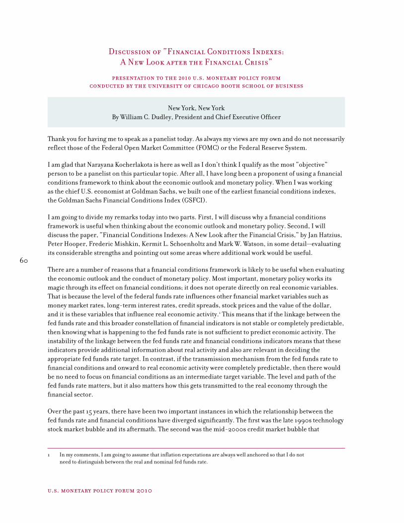
60


Thank you for having me to speak as a panelist today. As always my views are my own and do not necessarily reflect those of the Federal Open Market Committee (FOMC) or the Federal Reserve System.

I am glad that Narayana Kocherlakota is here as well as I don’t think I qualify as the most “objective” person to be a panelist on this particular topic. After all, I have long been a proponent of using a financial conditions framework to think about the economic outlook and monetary policy. When I was working as the chief U.S. economist at Goldman Sachs, we built one of the earliest financial conditions indexes, the Goldman Sachs Financial Conditions Index (GSFCI).

I am going to divide my remarks today into two parts. First, I will discuss why a financial conditions framework is useful when thinking about the economic outlook and monetary policy. Second, I will discuss the paper, “Financial Conditions Indexes: A New Look after the Financial Crisis,” by Jan Hatzius, Peter Hooper, Frederic Mishkin, Kermit L. Schoenholtz and Mark W. Watson, in some detail—evaluating its considerable strengths and pointing out some areas where additional work would be useful.

There are a number of reasons that a financial conditions framework is likely to be useful when evaluating the economic outlook and the conduct of monetary policy. Most important, monetary policy works its magic through its effect on financial conditions; it does not operate directly on real economic variables. That is because the level of the federal funds rate influences other financial market variables such as money market rates, long-term interest rates, credit spreads, stock prices and the value of the dollar, and it is these variables that influence real economic activity.1 This means that if the linkage between the fed funds rate and this broader constellation of financial indicators is not stable or completely predictable, then knowing what is happening to the fed funds rate is not sufficient to predict economic activity. The instability of the linkage between the fed funds rate and financial conditions indicators means that these indicators provide additional information about real activity and also are relevant in deciding the appropriate fed funds rate target. In contrast, if the transmission mechanism from the fed funds rate to financial conditions and onward to real economic activity were completely predictable, then there would be no need to focus on financial conditions as an intermediate target variable. The level and path of the fed funds rate matters, but it also matters how this gets transmitted to the real economy through the financial sector.

Over the past 15 years, there have been two important instances in which the relationship between the fed funds rate and financial conditions have diverged significantly. The first was the late 1990s technology stock market bubble and its aftermath. The second was the mid-2000s credit market bubble that

1 In my comments, I am going to assume that inflation expectations are always well anchored so that I do not need to distinguish between the real and nominal fed funds rate.

New York, New York By William C. Dudley, President and Chief Executive Officer

presentation to the 2010 u.s. monetary policy forum conducted by the university of chicago booth school of business

Discussion of “Financial Conditions Indexes: A New Look after the Financial Crisis”

61


culminated in the recent financial crisis. During these episodes, the relationship between the fed funds rate and financial conditions was particularly unstable. As a result, developments in the financial markets became very important in the conduct of monetary policy.

In this respect, I would note that financial conditions indicators have implications for “Taylor Rule” formulations for monetary policy. As you all know, Taylor-type rules provide a short-hand metric for the appropriate stance of monetary policy. In such rules, the fed funds rate is set at a level equal to the equilibrium real fed funds rate, plus the inflation objective, plus the weighted deviation of output from its potential and of the inflation objective from actual or, if forward looking, expected inflation. Often, analysts and economists assume that the equilibrium real fed funds rate is equal to 2 percent, its long-term historical value. Although, in principle, such rules allow the equilibrium rate to be time varying, it typically is assumed to be constant.

I have always been uncomfortable with this usage of a 2 percent equilibrium real rate assumption because it ignores the possibility that the equilibrium rate changes in response to technology shocks or in response to changes in how monetary policy is transmitted via the financial system to the real economy. For example, in the late 1990s, when trend productivity growth shifted upward, it seemed logical that this would also push up the equilibrium short-term real interest rate. That is because higher productivity growth, by raising the return on capital, spurs greater investment, thereby driving the equilibrium rate higher. Similarly, if stock prices rose sharply in response to higher productivity growth, this should also lead to a higher equilibrium real rate through the effect of greater stock market wealth on consumer spending. Higher stock prices meant that financial conditions were easier. This needed to be offset by a somewhat higher fed funds rate target.

Financial conditions also appear to have become more important in terms of their influence on business cycles. On the one hand, the fed funds rate has been more stable and the range of the fed funds rate over the cycle has been smaller. However, on the other hand, relative to what has happened to the fed funds rate target, financial conditions have become more volatile. The hypothesis that Ed McKelvey and I put forward in 1997 in response to evidence of the so-called “Great Moderation” seems to be well supported by the past two economic downturns and their aftermaths:

Put simply, longer stretches of economic growth imply greater leverage and complacency and thus, greater financial problems when recessions do occur. In brief, longer U.S. business cycles logically lead to four linked consequences—more financial leverage, longer bouts of balance sheet repair, more subdued recoveries and longer periods of decline in inflation and interest rates during the early stages of recovery.2

If the economy is more stable, then market participants will have more appetite for risk. This works fine during the expansion stage, when growth is relatively stable. However, when a recession finally arrives, it is a bigger shock than when recessions were more frequent. This surprise results in a more substantial adjustment in financial conditions. Ironically, the increased stability of the business cycle during the expansion phase appears to increase the volatility and importance of financial conditions when recessions do occur.

2 See The Brave New Business Cycle: No Recession in Sight, William Dudley and Edward McKelvey, January 1997, Goldman Sachs Economic Research Group.

62


At this stage, incorporating indicators of financial conditions into forecasting and into evaluating the conduct of monetary policy probably requires relying on constructing a “rough and ready” index. Macroeconomic models—especially dynamic stochastic general equilibrium models—do not incorporate robust financial sectors. Instead, these models have implicitly assumed that the monetary transmission mechanism and the financial intermediation process always works smoothly and predictably.3

Events of the past decade confirm that financial conditions matter and that the fed funds rate is not a sufficient statistic with which to assess the impact of monetary policy on the real economy. Of course, this is not news to the Federal Reserve, which has explicitly taken financial conditions into account in its conduct of monetary policy. This is evident in the transcripts of the FOMC meetings that are publicly available and the numerous references to financial conditions in the FOMC minutes that go back more than a decade.

An analysis of the FOMC minutes over the past decade indicates that references to financial conditions have been frequent, especially recently. Figure 1 illustrates the percentage of paragraphs in the minutes (excluding the directive and some other paragraphs associated with administrative matters such as the election of the chairman) that mention the phrase “financial conditions.” As can be seen, there have been frequent references over the past decade. One peak occurred in 2000 when the stock market peaked and began to deflate. Thereafter, references fell off a bit until rising sharply again recently. Clearly, the recent financial crisis has underscored the importance of financial conditions.

Today’s paper makes clear the importance of financial conditions. The paper’s analysis of the many financial conditions indexes that have been constructed as proxies for overall financial conditions finds that many of these indexes have done better than the fed funds rate or other single-variable financial indicators as predictors of real economic activity.

However, as the paper also makes very clear, the indexes that have been developed are still very rudimentary. In particular, most financial conditions indexes are ad hoc and incomplete. In their review of the existing financial condition indexes, the authors find considerable differences across the indexes in the way that they are constructed and in terms of the variables included.

In addition, there is another difficulty. As the financial system changes over time, both in terms of structure and in terms of financial products, the financial variables that we might determine to be important are also changing. For example, in the wake of the recent financial crisis, the variables that the paper’s authors call “neoclassical”—such as the yield curve and stock market prices—appear to have become less important relative to the variables that the authors term “non-neoclassical”—such as quantity and survey measures of credit availability. Variables that would work best 10 years ago as forecasting tools may no longer be very useful. As the structure of the financial system changes, the identity of variables that capture financial conditions naturally changes.

Let me now discuss the paper in more detail. I will do this in two steps. First, I will discuss the considerable contributions of the paper. Second, I will talk about where the paper might be extended and other areas of future research that might seem appropriate.

3 Adding financial intermediation to these models has become a very active area of research. See, for example, the recent work of Vasco Curdia and Michael Woodford in “Credit Spreads and Monetary Policy,” Federal Reserve Bank of New York Staff Report No. 385.

63


In general, I liked the paper. I think it makes some important contributions in how to construct a more complete and robust financial conditions index. In particular, I thought the paper makes two important points:

Financial conditions should measure financial innovations, not changes in financial variables that are due to past changes in economic activity. The endogenous components of financial conditions should be removed in the construction of a financial conditions index.

Both neoclassical (yield curve and stock prices) and non-neoclassical (credit availability) variables should be included. The GSFCI that I helped to develop only included neoclassical indictors and I think that was (and is) a shortcoming.

The authors deserve considerable credit for constructing a financial conditions index (FCI) that is more rigorous and complete than any that have been developed in the past—45 financial variables divided across five categories. Moreover, this is not just innovation for its own sake. The new FCI does a better job than single-factor models in forecasting real gross domestic product (GDP).

So what are the shortcomings of this approach? First, including 45 variables may generate good results more because the additional variables add greater flexibility to soak up variability in real GDP, rather than providing a more solid theoretical underpinning. As the authors note, the variables were selected, in part, on the basis of what we know today about which variables are likely to be important. But this type of selection process—even if conducted on a pseudo real-time basis—introduces selection bias, which the authors do admit could be important.

Second, despite the inclusion of a large number of variables, some important ones may still be missing. In particular, leverage variables—such as the leverage ratio of the major securities dealers—may be an important component of financial conditions. The work of Tobias Adrian and Hyun Shin suggests that the increase in leverage of the major securities was a major factor that fueled the asset bubble preceding the recent crisis. If this was indeed the case as seems likely, this type of variable should also be included in a financial conditions framework.4

Third, as the authors note, the resulting FCI is complex; it is difficult to estimate, update and to communicate what the results mean. I think FCIs have value as heuristic devices in highlighting what is important. One loses that benefit when the number of variables becomes large and the indexes become complex.

Fourth, it would be interesting to know how financial conditions indexes for other countries and regions would differ. The authors focus only on the United States. Thus, it is difficult to know whether the value of financial conditions indexes are specific to the United States or should be applied more broadly.

Fifth, I thought the paper could have gone further in exploring the implications of its results. The focus of the paper is on how to construct a financial conditions index that does a good job of forecasting economic activity. The paper does not tackle the implications for monetary policy stemming from developments in financial conditions as measured by the new FCI. If financial conditions evolve in an unanticipated way, how should this influence the conduct of monetary policy?

4 See, for example, Tobias Adrian and Hyun Shin, manuscript in preparation for the forthcoming Handbook of Monetary Economics, volume 3, currently circulated as Federal Reserve Bank of New York Staff Reports, No. 398, October 2009.

64


In particular, the authors note that during the 2003-06 period, financial conditions tightened less than expected given the rise in the fed funds rate and, during the 2007-08 period tightened even as the Federal Reserve slashed its fed funds rate target. These results raise a number of interesting questions. In particular, does the behavior of the new FCI imply that the Federal Reserve should have tightened more aggressively during the 2003-06 period or eased more aggressively during the 2007-09 period? The paper’s results seem to imply this, but it would be interesting to see whether this is the case or not.

It also would be useful to know how qualitatively important these differences are. If the differences are worth only a few basis points on the fed funds rate, then having a good indicator of financial conditions is not going to be a very important input in the formulation of monetary policy. In contrast, if a shift in financial conditions implies that the fed funds rate path was “off” by a hundred basis points relative to what actually occurred, then this obviously has big implications for monetary policy. The development of equilibrium models that incorporate financial conditions in a meaningful manner might prove helpful in answering these types of questions.5

In addition, I would like to know how the various linkages have changed over time. Is the linkage between the fed funds rate and financial conditions as measured by the new FCI loosening over time or not? If so, why is this happening? Is it due to financial market innovation or the growth in share of the non-bank financial sector? I also would like to know how the linkage between financial conditions and the real economy is changing over time. If this is happening, what are the implications for macroeconomic stability and monetary policy?

Finally, I would like to know about the dynamic properties of the new FCI. Are particularly high (expansive) readings dangerous and should they be taken as suggestive of asset bubbles? Should the Federal Reserve try to prevent such occurrences because loose financial conditions precede episodes of financial instability? In this respect, when financial conditions become unusually expansive, is the fed funds rate the right tool to use to constrain or counteract such expansiveness? Or would it be better to use macroprudential tools such as leverage limits or loan-to-value requirements on residential real estate to keep financial conditions from becoming unusually expansive in the first place? I could imagine circumstances in which macroprudential tools might be used to tighten up the relationship between the fed funds rate and financial conditions. Would the use of such tools be helpful in achieving greater macroeconomic stability?

At this stage, there are many more questions than answers. I would strongly encourage the authors and others to continue their work on financial conditions and in exploring how developments in the financial sector influence both the real economy and monetary policy. The financial crisis has demonstrated that financial market developments matter greatly. The paper successfully makes the case that it would be useful to have a good set of summary statistics to serve as benchmarks to keep track of such developments. It also would be useful to have a better understanding of how shifts in financial conditions should be considered in the ongoing conduct of monetary policy.

5 The work of Vasco Curdia and Michael Woodford referenced above is one step in this direction.

65


figure 1 “financial conditions” annual average % mentioned

Percent Percent

2000 2001 2002 2003 2004 2005 2006 2007 2008 20090

2

4

6

8

10

12

0

2

4

6

8

10

12

66


introduction

In this paper, the authors construct a new financial conditions index (FCI). As its name suggests, an FCI is a summary statistic that gauges how well financial markets are working. Before I continue, let me make the usual disclaimer and stress that the following views are mine, and not necessarily those of my colleagues in the Federal Reserve. The FCI in this paper has three novel features relative to earlier indices. First, it is constructed from a large number (45!) of distinct data series. These different series cover different sample periods (different beginning and end dates). The authors are able to use all of these distinct sources of information because they exploit relatively novel unbalanced panel estimation techniques to construct their index.

Second, the authors purge their FCI of information related to current and lagged GDP growth and inflation. They do so to better isolate information in financial markets themselves, as opposed to other parts of the economy.

Finally, prior FCIs are constructed to be the principal component of a number of underlying data series. Implicitly, these constructions are assuming that the underlying data series are largely driven by a single factor. The authors allow for the possibility that their 45 data series are generated by multiple factors (specifically three).

The authors use pseudo-out-of-sample forecasting exercises to evaluate their new FCI in terms of its ability to predict future GDP growth. Generally speaking, they find that the new FCI does somewhat better than a basic autoregressive (AR) model (in which lags of past GDP growth are used to forecast future GDP growth) and prior FCIs. The superior performance is especially pronounced in the past five years. However, the new FCI does considerably worse than these alternative models in the latter part of the 1990s.

I enjoyed reading this paper. I was especially impressed by how the authors exploited high-powered econometrics to combine information from so many distinct sources.

The authors focus on the use of the FCI as a forecasting tool. This is indeed an important question, and we learn much from their analysis. In my remarks, I will focus on a related but distinct question: How should we measure financial market conditions so as to best guide monetary policymakers’ decisions?

My discussion will begin with a brief—and certainly overly simplistic—description of three kinds of financial market frictions: collateral scarcity, asymmetric information, and illiquidity. (Admittedly, these terms are used in a variety of ways in the economics literature, and you will have to wait to hear how I’m

New York, New York By Narayana Kocherlakota, President, Federal Reserve Bank of Minneapolis


Discussion of “Financial Conditions Indexes: A New Look after the Financial Crisis”

67


using them.) Especially in light of the past two and a half years, it seems reasonable to think that the severity of these frictions may vary over time. I will argue, though, that the different frictions translate into different policy responses. As a result, economic theory strongly suggests that one needs more than a single variable to get a measure of financial market conditions that is useful for policymakers. I will try to provide some (crude!) guidance about how to parse the data to arrive at the relevant information.

three frictions

I discuss three frictions in asset markets and appropriate policy responses to their becoming more severe. Throughout, it is worth keeping in mind that government interventions typically have some administrative costs. These costs mean that interventions are certainly inappropriate when the frictions are relatively small in size.

Collateral

In frictionless credit markets, firms are fully able to capitalize their flow of future profits. In practice, lenders realize that borrowers may be able to hide or divert profits. As a result, a firm’s borrowing capacity is generally affected by the market value of its holdings of collateral. Appropriate notions of collateral vary from context to context. However, whatever their form, collateral requirements impose a connection between a firm’s ability to borrow and the market value of its collateral.

Thus, suppose that firms are using land as a form of collateral, and land falls in value by 20%. Then, some firms will be forced to forgo projects that they would have otherwise undertaken. The quantity of investment will fall. Perhaps more surprisingly, the equilibrium interest rate will fall. Intuitively, borrowers’ demand for loans is capped by the market value of collateral. A fall in the market value of collateral leads to a fall in loan demand. To equilibrate markets, the supply of loans must also fall— and that can only happen if interest rates decline.

There are a number of useful policy responses to collateral shocks of this kind. The problem is that firms don’t have enough collateral. Suppose that the government gives Treasury debt to all firms. Those with good projects now have a source of funding: They can sell their Treasury debt (or borrow against it). Of course, creating this new Treasury debt means that the government must tax in the future. However, as long as the credit constraint is sufficiently tight, the social losses created by this taxation are less than the gains generated by loosening the firms’ borrowing constraints.1

On the other hand, some seemingly useful policy responses are ineffective. Lowering the fed funds rate (and thereby the real interest rate) cannot generate more investment. Loan demand is constrained by the availability of collateral, not by the cost of funds to borrowers. Indeed, the above policy response (handing out more government debt to firms) necessarily raises interest rates.

Banks are firms, and so a good response may well require handing out Treasury debt to banks. Nonetheless, it may not be effective to give Treasury debt only to banks (as opposed to all firms). Banks will not be able to use this source of funds to make loans if firms are collateral-constrained.

1 These social gains exist because the government has a power that private lenders do not. The collateral constraint exists because borrowers can divert profits before repaying lenders. Governments can impose sales and other taxes that seize firm revenues before they can be diverted.

68


Asymmetric Information

Firms may have private information about their projects or their collateral. This private information confronts lenders with an extra form of risk and constrains their willingness to lend. Correspondingly, increases in private information lead to falls in the amount of lending and to spikes in the spreads between corporate lending rates and default-free Treasuries. Indeed, in extremis, private information problems can actually shut down lending entirely.

The government’s ability to respond to this friction depends critically on its level of information. If a government has no more information than lenders, then the government must lose money on any program that seeks to expand the scope of lending. (If this were not true, then lenders would have adopted that same program.) At least in this sense, taxpayers are made worse off by government interventions.

However, in some markets, governments may well have superior information to lenders. For example, through the bank supervision process, the Federal Reserve acquires a great deal of information that is not shared with markets. With this extra information, the Federal Reserve can safely lend through the discount window to potential borrowers at a lower rate than the borrowers would receive in private markets. There is a valuable synergy between the Fed’s role in bank supervision and its ability to intervene usefully in interbank lending markets.

Illiquidity

Financial markets vary in their liquidity. In liquid markets, a seller gets the same price per unit regardless of the quantity sold or the speed of sale. In illiquid markets, selling rapidly or selling a lot leads to large price per unit declines relative to selling slowly or selling little.

Liquidity shows up in asset prices and can influence allocations of real resources. For example, agency mortgage-backed securities (MBSs) issued by Fannie Mae and Freddie Mac are guaranteed against default risk. But they still contain prepayment risk. The buyers of agency MBSs can usually diversify much of this risk by selling the asset. Now imagine, though, that the secondary markets for agency MBSs become much less liquid. Buyers of agency MBSs cannot diversify away the associated prepayment risk, and so demand a higher yield per unit of risk held. (Technically, we say that the market price of agency MBS prepayment risk rises.) Agency MBS risk premia rise, and home buyers end up facing higher mortgage rates.

The government can respond usefully to such an event. Suppose that the government buys a large amount of MBSs. Their generated flow of income will not greatly affect the government’s revenue stream, and so the government faces relatively little additional risk by buying the MBSs. However, buyers now have to hold a lot less risk in the form of agency MBSs. The market price of agency MBS prepayment risk declines. This form of government intervention is desirable because the government can cheaply diversify its position, while a private agent cannot.

If the market remains illiquid, then government sales of agency MBSs would lead to increases in their risk premium (because MBS buyers are forced to hold more risk). But eventually, the agency MBS market will become liquid once more. At this point, the government can reverse its operation and sell its MBSs in secondary markets without affecting their risk premium.

69


how do we see the frictions in the data?

I have talked about three frictions and the associated policy responses. Admittedly, the frictions almost certainly overlap to a greater extent than my discussion implies. For example, markets may well become more illiquid when collateral constraints tighten and/or private information problems worsen.

But, in general, these are three distinct frictions with three distinct policy responses. A single FCI cannot capture their separate fluctuations. To understand appropriate policy responses, one needs to identify (at least) three distinct financial condition factors (FCFs).

I think that the authors do a useful first step in this direction. In Table 5.2, they distinguish several FCFs based on subsets of their 45 data series. They document that these FCFs do not have superior predictive performance relative to their preferred FCI. However, this exercise could be made even more useful by using theoretical considerations to map various kinds of credit market frictions into distinct choices of subsets of variables.

My discussion of the various frictions provides some initial insights into how we can determine their relative severity using financial markets data. For all of them, of course, we should see loan quantities decline. How else would they show up in financial markets data?

Friction 1 (collateral): Collateral prices fall, and interest rates decline. Credit market risk spreads do not change.

Friction 2 (private information): Credit market spreads increase, and loan standards tighten.

Friction 3 (illiquidity): The market price of a given asset’s risk rises.

I have to say that separate frictions are probably not essential in thinking about the period from late 2007 through mid-2009. It seems clear—both from the authors’ work and from more casual empiricism—that all three of these frictions increased greatly in severity during this period.

But the current picture is murkier. I would certainly say that at this point, credit market spreads are sufficiently low that friction 2 seems hardly relevant. It is harder to tell about friction 3. The market price of agency MBS prepayment risk has fallen, but this decline may well be due to the large Fed holdings of agency MBSs.

But net borrowing remains low. This indicates to me that friction 1—low borrowing capacity because of collateral constraints—may still be significant. Both short-term and medium-term real interest rates (as measured by TIPS bonds) are low relative to their historical averages. Land is an important source of collateral, and its price remains low. (More generally, as of 2009:3, nonfinancial noncorporate net worth is down about 17% from 2007.) It is true that credit market spreads have vanished, but this is not a relevant consideration when thinking about friction 1.

70


It is exactly this kind of analysis that makes me think that using multiple FCFs to gauge financial market conditions might be so important. This point is reinforced by the recent behavior of the eight FCIs in the authors’ paper. The first seven all rose in the second half of 2009, but the authors’ own FCI fell. Clearly, there are at least two distinct factors responsible for these movements. My message is that knowing these distinct factors matters for understanding how policymakers should respond to worsening financial market conditions.

Conclusions

In many ways, my remarks parallel the sophisticated discussion of financial market imperfections in the introduction to this paper. To use their language, the authors point out that our modeling of such imperfections is still rudimentary. They argue that this state of play means that one has to use reduced-form statistical techniques to create FCIs.

I agree with them that the extant modeling is rudimentary, and it is likely to remain so for some time. Nonetheless, even these simple models have important insights. I hope that these model-based insights become more central in future attempts to construct measures of strains in financial markets.

71


By Anil K Kashyap1, University of Chicago Booth School of Business, NBER and Federal Reserve Bank of Chicago

I will not start by thanking myself for putting me on this panel. But I would like to thank Dave Wessel, Governor Tarullo and President Evans for participating. The normal temptation for an academic who gets an audience with such a distinguished group of policymakers is to promote one’s latest and greatest new idea. But having tried that on numerous occasions with pretty limited success I am going to take a differ tact. Instead, I am going to say some things that I think many and perhaps most policymakers already understand and agree with, but perhaps feel uncomfortable pushing. So I am going speak primarily to the members of the audience who are not policymakers and especially the press to try to change their thinking on the so-called Volcker rule.

In particular, I will make a frontal assault on the wisdom of having the Volcker rule as the headline feature of regulatory reform efforts. For these purposes I will define the Volcker rule as restricting banks from making speculative investments that do not benefit their customers. I want to attack it on theoretical grounds, question its empirical relevance, and explain why I believe it is even bad politics.

Theoretical Considerations

Starting with the theory, there are fundamentally two theories of what banks do and why they are special. One emphasizes the role that banks play in monitoring customers who want to borrow money. The other stresses the importance of offering liquidity on demand.2 When thinking about regulating banks it is critical to decide which of the two motives matters. I want to stress the liquidity provision theory and think about its implications.

Let’s take perhaps the simplest version of that theory. It is based on the proposition that there is an underlying demand for payment services that someone must offer. It can be summarized as saying we have checking accounts because using them is much more efficient than carrying around large amounts of cash. So there is an intrinsic demand for debit type payment options.

Now let’s think about how this preference will be met. To successfully offer demand deposits, a bank needs ready access to funds and to develop the infrastructure to predict when cash will be withdrawn. But notice that solving this problem is identical to figuring out when a customer might draw on a line of credit. For the bank, it makes little difference whether money is flying out the door because a customer writes a check or draws on a commitment. Either way, the bank has to have the money ready.

1 These remarks are my own personal views and should not be associated with the organizations with which I am affiliated.

2 A lot of recent work by my colleagues, Douglas Diamond and Raghu Rajan, try to put the two together.


Let’s Not Pursue the Volcker Rule

72


But this means the same buffer stock of funds that a bank would hold to service checking withdrawals allows it to also offer loan commitments. So it will necessarily be cheaper for banks to offer each product than any other organization that was only offering one of the two products.

This theory explains lots of banking regularities, both historical and current. Most importantly, it explains why since medieval times banks have always offered overdraft protection (the historical version of a loan commitment). But it also explains why, looking across banks, those which are more deposit-intensive tend to offer more commitments.

Finally, it explains why in a crisis the banking system can be a source of stability. During many times of stress a flight to safety pushes people to move their money into the banking system. This inflow delivers cash to the banks exactly when some of their customers may need to borrow, so the banks can continue lending. This pattern was carefully documented in the Asia financial crisis.

Why does this perspective on the banks matter for regulation and the Volcker rule? First, it is fashionable to talk about narrow banks that only offer deposits and invest in safe securities. This seems like the simplest and most direct way to stop the banks from needing bailouts and contributing to economic instability. The theory explains why we do not see these types of banks occurring naturally. It also tells us that splitting the lending operations and deposit-taking operations would entail major efficiency costs. For the same reasons why insurance companies want to offer insurance on different types of risks, banks find it efficient to take deposits and offer commitments.

Second, the lending side of the bank may naturally want to hedge certain types of risks that emerge once a loan commitment is drawn upon. For instance, this might include eliminating foreign currency risk, or interest rate risk. There is no good reason to ask the banks to shoulder these risks. How theoretically is the Volcker rule to be applied to identify these worthy hedging activities and separate them from gambling?

Empirical Relevance

Let me know move away from my theoretical concerns and turn to some empirical problems.

First, measuring the importance of proprietary trading is challenging. There are no published financial statements that allow us to separate this activity from total trading revenue. Direct measurement of this part of the business is therefore impossible. But, based on what the banks say, they believe proprietary trading to be small. For instance, Goldman Sachs’ CFO estimated that about 10% of their trading revenue was from “walled-off proprietary business that has nothing to do with clients.” Bank analysts have used that number to extrapolate to other large institutions (which generally have less trading revenue than Goldman). For example, a report by Wells Fargo estimates that Morgan Stanley would have roughly 3 to 4 percent of revenue from prop-trading and Bank of America and JP Morgan would have less than 2 percent.

Of course, if one wants to cast a wide net to say clients do not benefit from anything involving a derivative security, then the magnitude of the alleged gambling is much larger. But in this case, then the concern over killing all hedging becomes paramount.

73


Second, let’s look back at the central problems for the financial system and the main costs to the taxpayer from this crisis. They have had virtually nothing to do with proprietary trading by banks. Under the Volcker rule, the problems at Bear Stearns, Lehman Brothers, and AIG would have been identical to what we saw. These institutions would have been exempt from restrictions on their activities. If we learned anything from the crisis it is that firms that are deeply inter-connected to the financial system can wreak havoc, regardless of their size, and that the inability to gracefully wind down such firms is a major shortcoming of the current system.

Third, if we were to restrict activities, the crisis suggests that the obvious place to focus is on Prime- Brokers. I hope none of the people in this room are still trying to recover their money from Lehman’s UK brokerage, but it would not surprise me if someone were in that position.

In the Lehman bankruptcy we learned the extent to which a broker was using securities (and extra collateral) provided by clients to support lending. As Lehman got into trouble some clients pulled their money and this forced Lehman to contract (or find new funding). Once the failure occurred some clients were not able to recover their securities.

There is a vigorous debate currently underway as to whether client assets should be segregated from the broker’s funds. This would certainly have made the failure less traumatic. But it also would force assets that could circulate in the market providing other services, for example for shorting purposes or to back further secured loans, to sit idle.

Because of this tradeoff deciding how far to go regarding segregation is challenging. But I think there is no doubt that if we want to talk about limits on bank activities this is THE area to be discussing.

Political Considerations

Finally, let me close by explaining why I think all the attention on the Volcker rule is also bad politics.

I see a close analogy to the TARP debate. Remember that initially it was sold as request for Congress to allow the Treasury to buy toxic assets. Many of us kept asking for an explanation as to how this would work, while arguing instead that a capital injection for the banks was needed. When the Treasury changed its mind and switched course, the public and the politicians felt misled and lost confidence in the process. (As Alan Blinder likes to point out, the public’s band width on these matters is pretty limited: he notes that because the TARP request was for 700 billion and the stimulus was 787, so that both figures started with a 7, the average person can’t tell them apart! I think he is right.)

Once again we see that the administration’s headline recommendation does not pass the sniff test – no one can explain how the Volcker rule would have helped in the last crisis, and the reason, as I just explained, is that it wouldn’t. On the other hand, I think all experts would tell you that getting resolution authority would make a huge difference. The next time a Lehman event looms we want to be able to have many more tools to use to fail the firm or to sell it off more smoothly. The fact that we do not have any better options than we did in September 2008 is a major disappointment.

I am sure that people from the administration would claim I am being unfair and that the Volcker rule is just one part of its package of reforms and that they want resolution authority too. Technically speaking that is true. The administration has put out several reform proposals, including some that are pretty comprehensive and that I would be prepared to support.

74


But the details on this legislation are critical and as the President is fond of pointing out there are many entrenched interests who oppose reform. The global linkages in the financial system mean that many of the reforms require international cooperation that will take sustained efforts. I think harmonizing bankruptcy rules will be a task measured in years. For this reason, it is essential to focus on getting started on this immediately before the next crisis.

The Volcker rule is particularly bad on this front because it is so easy to remember: diagnosis, the banks were gambling, solution, we need to stop it. Who can be against this idea? The public is sure to remember this idea.

Keep in mind also, the way international meetings work. Much of the task of financial reform has fallen to the Group of Twenty nations. There will be meetings later in the year where heads of state gather to discuss financial reform and various other issues. Imagine the table where all 20 leaders are seated and they each take turns to start the meeting by giving 6 minutes of opening remarks – this means it takes 2 hours just to finish introductions! If the Americans keep pushing this kind of reform, then it is guaranteed that this will be on agenda. What elected leader will be able to pass up the chance to beat up the banks over their reckless gambling? Most politicians would rather go to the dentist than talk or think about financial regulation reform. So once they are given the chance to rail against reckless bankers that will be the end of the discussion – it will simply suck the oxygen out of the room. Serious reform discussions will be totally crowded out.

So while I admire Paul Volcker and I thank him for many contributions to central banking, on this issue I hope he does not succeed. Instead, I hope the next time the President wants to talk about financial regulatory reform, and he needs a sound bite, he switches to talking about putting financial institutions through bankruptcy and how it is not fair that the man on the street can be taken to bankruptcy court, but large banks can’t. I think that is a message that would resonate but would be much better priority.

Thanks for your attention.

75


Evans: It’s a pleasure to be here. Today, I would like to offer a few comments on regulatory reform with a slightly different perspective from that which has been presented so far in the conference.

We’ve had a number of similar conferences in Chicago in recent years that were devoted to the financial crisis: Our Bank Structure Conference, the Fall International Financial Conference and others. Often I am frustrated by presentations that offer smart criticism without constructive commentary. Although the criticism by itself is useful, I would like to propose that we require our invited experts to put something explicitly constructive on the table.

I may not deliver on that myself just now, but I will do my best to put forward some comments specifically related to the current discussion on macro-prudential regulation. Today, I would like to offer my thoughts on some of the reform proposals that are being discussed. I should note that my remarks reflect my own views and are not those of the Federal Open Market Committee or the Federal Reserve System.

We are slowly emerging from the worst financial crisis since the 1930s. The hardships created by these exceptional circumstances for households and businesses are well known. Governments and regulators around the world have responded to the crisis with a variety of aggressive and innovative policy actions, including giving special assistance to specific institutions.

Now, we are engaged in a vigorous debate on how best to address the major weaknesses in our financial regulatory framework that were revealed by the crisis. Our goal, clearly, is to avoid another crisis of this magnitude. Financial reform will not be easy. We face complex problems that will require a comprehensive, multi-pronged approach. But reform is critical for ensuring our long-term economic stability.

To highlight some of the changes that are being considered, there are proposals that would assign monetary policy a more active role in fighting asset bubbles; proposals that would strengthen current microprudential regulations; proposals that would introduce a systemic regulator and macroprudential regulations; and proposals that would create resolution authority – particularly for systemically important financial institutions.

Time does not permit me to discuss the specifics of each of these proposals today. Instead, I would like to offer my thoughts on some of the challenges we are likely to face in implementing even the most well-thought-out policies.

Let me be clear. I don’t bring up these potential challenges as roadblocks to the healthy debate that is underway. Rather, I offer them as issues we need to consider as we build a better financial infrastructure.

One preemptive action that is being debated concerns the role of monetary policy in combating asset bubbles. Given the rapid rise in some asset prices prior to the recent crisis, there are increasing calls for

By Charles L. Evans, President, Federal Reserve Bank of Chicago

Panel Discussion, U.S. Monetary Policy Forum, February 26, 2010


76


central banks to be more proactive in responding to signs that an asset bubble may be emerging and to raise their target rates in order to lower asset prices that, by historical standards, seem unusually high. In previous forums, I have discussed why I view these proposals with skepticism.1 I won’t cover the same ground here again. Instead, let me just note that I am skeptical about our ability to easily and definitively sort out in real time whether a rapid increase in asset prices is associated with overvaluation. That is, how confidently can we state that we are in the midst of a bubble? I also think that monetary policy is too blunt a tool for pricking bubbles: It can’t be targeted precisely and it will affect other financial and macroeconomic variables in addition to the suspected bubble asset. In addition, the typical changes in interest rates that a central bank might contemplate are likely to be too small to produce big changes in asset prices.

Fortunately, monetary policy is not the only tool that policymakers have to deal with financial exuberance. In my view, redesigning regulations and improving market infrastructure offer more promising paths. Regulation may or may not be sufficient to avoid all of the events that create crises, but it should go a long way toward doing so. Better supervision and a sound regulatory infrastructure can also increase the resiliency of markets and institutions and their ability to withstand adverse shocks that do occur.

Within the existing structure, regulators have the ability to promote better, more resilient financial markets, either through rule-making or by serving as a coordinator of private initiatives. They can also encourage more and better disclosure of information—a key element of effective risk management. A number of initiatives along these lines have been taken and additional ones are being considered.2

We can use existing regulatory tools more effectively, but we also need to address the shortcomings of current regulations. The ongoing work of the Basel Committee on Banking Supervision regarding the possible introduction of liquidity standards and adjustments to the existing capital requirements are examples of such efforts.

While such enhancements to micro-prudential regulations are necessary, I would argue that they are not close to being sufficient to address the complex issues we faced during the recent crisis. Success in preventing and controlling potential risks requires very early and courageous action by policymakers. Typically, risks and problems in the financial system build over a number of years. There is an awful amount of uncertainty as to whether risks are developing; how they will be perpetuated; and when to take action. Microprudential regulations alone are not likely to resolve these issues.

Let me illustrate the sort of problems a microprudential regulator faces with a specific example. As you know, the problems with residential mortgages, particularly with subprime mortgages, were one of the key areas that precipitated the current crisis. Currently, the U.S. financial system faces problems with commercial real estate (CRE) loans. At the end of 2009, depository institutions in the U.S. held over $1.5 trillion in commercial real estate and construction loans on their books. In addition, there are currently nearly $800 billion in commercial mortgage-backed securities (CMBS) outstanding. Over the past two years, delinquencies on these loans and securities have been rising at an uncomfortably rapid rate.

1 For instance, see Evans (2009a and 2009b).

2 For instance, in recent years, regulators have actively supported the development of the Trade Information Warehouse (a central repository for trade reporting of over-the-counter credit derivatives contracts) and clearing houses for credit default swaps, such as ICE Trust.

77


Figure 1 shows that of the over $1 trillion in commercial real estate loans held by depository institutions today, nearly 4 percent are noncurrent.3 This ratio was about 0.5 percent before the crisis (June 2007). The picture is even worse for the riskier construction and land development loans. While these loans total less than $0.5 trillion, the noncurrent portion had risen from 1.5 percent at the end of June 2007 to nearly 16 percent by the end of last quarter. For CRE loans packaged into securities, serious delinquencies represent 4 percent of all CMBS currently outstanding, up from nearly zero before the crisis.

Does such a fast rise in CRE and CMBS delinquencies mean that bank examiners missed clear signs of forthcoming problems and failed to take action? Commercial real estate loans are a key problem area for the banks in my District. I went to my supervisory staff and said: “I know you are struggling with commercial real estate loan portfolios. What are the difficulties? What do you think we needed to have done in the past in order to avoid the current problems?”

I have to admit that their response made me pause. They said “You know, Charlie, if we wanted to avoid the current situation, we needed to act very, very early – probably in 2004 or 2005.” That is a full two to three years before the onset of problems in the sector. Clearly, we needed to act very early. But at that time, it would have been difficult to argue convincingly in favor of reigning in this lending. The economy was coming out of the jobless recovery and just beginning to gain traction. And the banking industry had proven it could maintain profits through a recession, it had reduced problem loans back to historically low levels, and it appeared to have more than sufficient capital to cushion against potential losses.4

Given previous problems with commercial real estate loans, my supervisors understood the potential risks. Here is a typical situation they faced. Imagine you are an examiner and you go out to review a large financial institution in 2005. The institution is warehousing commercial real estate loans prior to securitization during a period when CMBS issuance is just taking off and, for every $1,000 in CRE loans, only $6 are noncurrent. Nonetheless, as an examiner, you have a discussion with the bank managers and you learn about their lending practices, and you kind of wonder, “How well-controlled is all of this?”

The loan officers will give you some very good arguments about what their business is and how the risks are being controlled. First, they are not really storing the loans on their books. They are underwriting the loans with the full intention of packaging them into securities. They have to build up a critical mass before securitization, but they are not going to keep the loans.

From the banks’ perspective, they are not in the storage business. They are in the transportation business. It is rather short term – 60, 90 days. Presumably, the risk is only proportional to how long they are holding on to it – which is not very long. Furthermore, during this period, real estate prices are going up, delinquencies are negligible, and banks have a variety of hedges in place. They look at commercial real estate prices and think, if needed, they can get out of their portfolio at little cost. And even if some losses materialize, they have adequate capital.

3 Noncurrent loans are those that are 90 days or more past due plus loans in nonaccrual status.

4 At the end of 2004, return on equity at all commercial banks in the U.S. was 13.08 percent, near its historical peak of 16.23 percent in the second quarter of 1993. Return on assets were similarly high, and net charge-offs accounted for only 0.68 percent of total loans, well below 1.31 percent reached at the end of 2001.

78


I have some interesting people on my staff who can push back in a pretty challenging fashion. But at the end of the day, after carefully considering the banks’ arguments, they think: “All right, I guess the loan officers are looking at this pretty reasonably and are protecting their institution.” And the risk to the deposit insurance fund from all this activity seems pretty small. So, you end up being convinced that the activity is probably okay.

Today, with hindsight, we know that while most of the micro risks appeared very small at the time, their sum was far less than the macro risk that was silently building up. That’s the key thing: A collection of negligible micro risks can add up to a far greater macro risk. Focusing on individual institutions and controlling risks on a firm-by-firm basis are not enough for detecting and controlling system wide stress points.

That is why we need macroprudential supervision and regulation. Suppose for a particular class of assets, values decline on an economy-wide basis. This means losses are going to be taken at the macro level. Perhaps managers at a few individual banks can be smart, foresee the price declines, and liquidate their positions in time to avoid large losses at their institution. But the macro economy has to take these losses, and that’s where we get stuck. Not everyone can get through the exit door at once; someone has to end up bearing the macro losses.

This is why macroprudential regulations that aim to assess and control systemwide risks should play a critical role in our regulatory structure. For instance, dynamic capital requirements and loan loss provisions that vary over the cycle can temper some of the boom–bust trends we have seen in the past. History shows that during boom times, when financial institutions are perhaps in an exuberant state, they may not price risks fully in their underwriting and risk-management decisions. During downturns, faced with eroding capital cushions, increased uncertainty, and binding capital constraints, some institutions may become overcautious and excessively tighten lending standards. Both behaviors tend to amplify the business cycle. Varying required capital loan loss provisions over the cycle could serve to offset some of this volatility.

We saw the advantages of a systemic, macroprudential approach firsthand during the implementation of the Supervisory Capital Assessment Program (SCAP) – the so-called “stress tests.” Last spring, the Federal Reserve led a coordinated examination of the largest 19 U.S. banks. We reviewed the institutions simultaneously, applying a common set of assumptions and scenarios across all of them. Such an approach provided us with a view of these banks in their totality, as well as the financial condition of individual institutions on a stand-alone basis. The horizontal view was essential in assessing how risks taken individually by each bank are correlated and how they can add up to more than the sum of individual components. The review also had a forward-looking element that assessed the likely condition of the banks under a specific set of adverse economic conditions and determined the amount of capital the banks would need under these “stress” conditions. Such procedures also enable supervisors to identify best practices in risk management and to push banks with weak controls to improve and adopt these industry best practices. Indeed, supervisors at the Federal Reserve have already begun to adopt such an approach.

79


However, even with such macroprudential strategies, we are going to face challenges. Let’s think about what, as a hypothetical macroprudential regulator, we would have to do. What should be the early call focus? What should we be looking at? When should we be looking at it? How confident are we that that we are actually going to be able to identify the problem? A macroprudential regulator is confronted with the same type of questions a microprudential regulator faces, but at a systemwide level.

Consider these questions within the context of commercial real estate. The facts are, today, CMBS and CRE loans have large delinquencies. Could anyone have made this call confidently in time to arrest the problems we face today?

Recall that the outstanding volume of CMBS ramped up in 2004, 2005. At the same time, commercial real estate prices (shown in the top panel of Figure 2) continued to rise well into 2007. On the bottom panel, we see the performance of loans originated during this period, depending on when the loans were made. Loans originated later in the credit cycle are performing worse than older loans. For instance, loans underwritten in 2005 did not reach a 1 percent delinquency rate until about 42 months (3.5 years) after origination. In contrast, loans made in 2008 reached the 1 percent delinquency mark only six months after origination. The progressively worsening performance of loans originated later in the credit cycle is likely due to looser underwriting standards that supported the issuance boom.

With the benefit of hindsight, I can point to the inflection point in volume and say “I should have put my finger on that right then.” At that point in the credit cycle, “shouting” would have been an important part of risk-control, as it would have emphasized potential risks to the market players.

But I can’t imagine that supervisors’ concerns would have been taken seriously in 2005 or 2006 – even if they started going out and shouting to the heavens that there is a big, big problem and we need to do more about it. Recall that, at that time, real estate prices were ramping up and delinquencies were low. Indeed, in 2007, the Federal Reserve, along with other bank regulators, issued a supervisory guidance on concen-trations in commercial real estate.5 We also gave a number of speeches prior to the crisis about risk pricing and about market exuberance – to little avail. These warnings were largely ignored and we got a lot of push-back from banks. During boom periods when risks are silently building up, there are a lot of people with a lot of money at stake who will come out against such pronouncements. So, if policymakers do not follow words with actions, then we are not likely to make much progress. Shouting and supervision – together – are essential.

I raised some potential issues with both micro- and macro-prudential regulations. How do we address these issues? This is where we would take full advantage of our multi-pronged approach to regulatory reform. If we are not certain that a particular approach may not be as effective as we would like, we can put more pressure on other levers to obtain a desired amount of risk control. So, if we think that macro-prudential regulations may have some potential operational issues, we would need to implement more stringent capital and liquidity requirements than we would otherwise to overcome these issues.

5 See, “ SR 07-1 Interagency Guidance on Concentrations in Commercial Real Estate” available at http://www.federalreserve.gov/boarddocs/srletters/2007/SR0701.htm(external). More recently, the Federal Reserve issued a supervisory guidance on managing interest rate risk (“SR 10-1 Interagency Advice on Interest Rate Risk,” available at http://www.federalreserve.gov/boarddocs/srletters/2010/sr1001.htm(external)) and highlighted it in speeches (for instance, see Kohn (2010)). In addition, the Federal Reserve - along with the other Federal banking agencies - issued a policy statement on funding and liquidity risk management on March 17, 2010 (available at: http://www.federalreserve.gov/newsevents/press/bcreg/20100317a.htm).

80


This is why we need a multi-pronged approach to a robust regulatory structure: a structure that takes full advantage of the existing tools supervisors have; a structure that supplements the existing one with dynamic capital requirements and a comprehensive approach to risk management; a structure that includes a macroprudential supervisor than can monitor and assess incipient risks across institutions and markets and, when necessary, impose higher regulatory requirements on firms that pose systemic risks.

However, even with such a structure, it would be hubris on the part of policymakers to assume that we would be able to prevent financial stress at all financial institutions. Therefore, we also need to contain the disruptive spillovers that result from the failure of systemically important institutions without resorting to bailouts or ad hoc rescues. A necessary element of this is having a mechanism for resolving the failure of a systemically important institution.6 This is something we currently lack in many cases, though there are proposals now under discussion that would provide this resolution power.

Another issue that arises in the regulatory reform debate is whether the central bank should be entrusted with supervision and regulation responsibilities. There are many synergies between monetary policy and supervision and regulation that I and others have discussed in previous speeches.7 Let me point out a couple of reasons why it might be optimal for a central bank to have a key role in financial stability and regulation.

The reality is that central banks have the unique ability to act as the lender-of-last-resort during financial crises. The central bank cannot use this tool effectively if it is not knowledgeable about the financial condition of the institutions it might lend to, particularly if such loans need to be made at very short notice.

The lender-of-last-resort role inevitably thrusts the central bank into efforts to promote financial stability and avoid crises. If, however, central banks have no supervision and regulation tools, they are constrained to act with the only tool at their disposal – monetary policy.

I already mentioned that I am skeptical about using monetary policy to control financial exuberance. But without supervisory powers, there may be no choice. We know that time consistency issues can lead a central bank to choose inflationary outcomes in the short run, even though there is no long-run tradeoff between output growth and price stability. Ken Rogoff pointed out that one way to deal with this issue would be to appoint a conservative central banker who would be tougher than the public. This would ensure that appropriate decisions would be made and appropriate actions would be taken.

Now, consider the reaction function of a central banker that has the additional responsibility for financial stability – but not the additional tools provided by a supervision and regulation role. Such a central banker might have to act against exuberance in financial markets more actively than it would otherwise. That would be entirely necessary and appropriate to preserve financial stability. However, that policy may not be the most appropriate one at that time for addressing the traditional goals of monetary policy of maximum sustainable employment and price stability. A central bank with three goals and only one lever is a recipe for producing some difficult policy dilemmas.

6 See Evans (2009c) for my views on the advantages of resolution authority and the issues it would address.

7 For instance, see Bernanke (2010), Evans (2010), Kashyap (2010), and Volcker (2010).

81


To sum up, it is clear that, in order to avoid a situation like the one we have faced in the past two years, we need to fortify our regulatory lines of defense. We need to change the rules of regulation to be more efficient and effective in their design and implementation. But we also need to openly acknowledge the challenges policymakers and regulators are likely to face in containing potential financial crises. Despite all the challenges, I believe that we can design a more effective regulatory structure through discussions such as the one we are having today.

Thank you.

figure 1 commercial real estate (cre)

Noncurrent Loans/Total Loans*(Percent)

Noncurrent Loans/Total Loans*(Percent)

*Noncurrent loans are loans that are 90 days or more delinquent plus loans in nonaccrual basis. For CMBS, the delinquency rate shown is for loans that are 60 days or more delinquent.

2007 Q22009 Q4

0

5

10

15

20

0

5

10

15

20Construction and Development Loans

(Outstanding: $452 billion)CRE Loans

(Outstanding: $1,091 billion)CMBS

(Outstanding: $800 billion)

82


figure 2 commercial real estate - cmbs

Real Estate Prices(MIT Center for Real Estate Commercial Index)

CMBS Delinquencies by Vintage(60+ days delinquent as a percent of CMBS conduit since month of origination)

Percent

50

100

150

200

250

50

100

150

200

250

1999 2000 2001 2002 2003 2004 2005 20102006 2007 2008 2009

1 6 11 16 21 26 31 36 41 46 51

Q4 2009

Feb 2009

0

2

4

6

0

2

4

6

Source: Trepp LLC

20052006

20072008

83


References

Bernanke, Ben S., 2010, The Federal Reserve’s Role in Bank Supervision, Testimony before the U.S. House Committee on Financial Services, Washington, DC, March 17. http://www.federalreserve.gov/newsevents/testimony/bernanke20100317a.htm

Evans, Charles L., 2009a. “The International Financial Crisis: Asset Price Exuberance and Macroprudential Regulation.” Remarks given at the 2009 International Banking Conference on September 24, 2009 in Chicago, IL. Available at: http://www.chicagofed.org/webpages/publications/speeches/2009/09.24_IBC_speech.cfm

Evans, Charles L., 2009b. “Should Monetary Policy Prevent Bubbles?” Remarks given at the ‘Asset Price Bubbles and Monetary Policy” Conference on November 13, 2009 in Paris, France. Available at: http://www.chicagofed.org/webpages/publications/speeches/2009/11.13_BoF_speech.cfm

Evans, Charles L., 2009c. “Too-Big-To-Fail: A Problem Too Big to Ignore” Remarks given at the European Economics and Financial Center on July 1, 2009 in London, England. Available at: http://www.chicagofed.org/webpages/publications/speeches/2009/07.01_EEFC_Speech.cfm

Evans, Charles L., 2010a. CFA Society of Chicago Distinguished Speaker Series: Luncheon Economic Forecast.” Remarks delivered on March 4, 2010 in Chicago, IL. Available at: http://www.chicagofed.org/webpages/publications/speeches/2010/03_04_CFA_speech.cfm

Evans, Charles L. 2010b, CFA Society of Chicago Distinguished Speaker Series: Luncheon Economic Forecast, March 4. http://www.chicagofed.org/webpages/publications/speeches/2010/03_03_CFA_speech.cfm

Kashyap, Anil K, 2010 Examining the Link between Fed Bank Supervision and Monetary Policy, Testimony before the House Financial Services Committee, March 17. http://www.house.gov/apps/list/hearing/financialsvcs_dem/kashyap.pdf

Kohn, Donald L., 2010. “Focusing on Bank Interest Rate Risk Exposure.” Remarks delivered at the Federal Deposit Insurance Corporation’s Symposium on Interest Rate Risk Management on January 29, 2010 in Arlington, Virginia. Available at: http://www.federalreserve.gov/newsevents/speech/kohn20100129a.htm(external)

Volcker, Paul, 2010, Statement, Testimony before the House Financial Services Committee, March 17. http://www.house.gov/apps/list/hearing/financialsvcs_dem/kashyap.pdf

84


It is a pleasure to participate in this year’s U.S. Monetary Policy Forum. To begin the discussion of regulatory reform, I will first explain my view that the imperative for financial regulatory reform has much deeper roots than the imprudent mortgage lending, tightly wound wholesale financing channels, and other factors that were direct contributors to the recent financial crisis. Next, I will summarize the status of the reform proposals to address systemic risk, as well as the changes that are already in train, before ending with a few observations on the relationship between the scope of the systemic risk problem and the reform agenda.

The Roots of the Financial Crisis

It is interesting and important to inquire carefully into the immediate causes of the financial crisis. But an appropriately tailored response must begin by recognizing that the crisis arose following profound changes in both the organization and regulation of financial markets that began in the 1970s. Starting in 1933, the New Deal established a regulatory system that largely confined commercial banks to traditional lending activities within a circumscribed geographic area, with attendant limits on price competition and a federal deposit insurance backstop meant to forestall bank runs. This approach fostered a commercial banking system that was, for the better part of 40 years, quite stable and reasonably profitable, though not particularly innovative in meeting the needs of depositors and borrowers.

The turbulent macroeconomic developments of the 1970s, along with technological and business innovations, helped produce an increasingly tight squeeze on the traditional commercial banking business model. The squeeze came on both the liability side of bank balance sheets, in the form of more-attractive savings vehicles such as money market mutual funds, and on the asset side, with the growth of public capital markets and international competition. Large commercial banks reacted, among other ways, by seeking removal or relaxation of the regulations that confined bank activities, affiliations, and geographic reach--a request to which supervisory agencies and legislators were generally sympathetic because of the potential threat to the viability of the traditional commercial banking system.

The period of relative legal and industry stability that followed the New Deal legislation thus gave way in the 1970s to a nearly 30-year period during which many prevailing restrictions on banks were relaxed, both through administrative action by the bank regulatory agencies and through a series of legislative changes culminating in the Gramm-Leach-Bliley Act of 1999. By the turn of the century, the Depression-era cluster of restrictions on commercial banks had been replaced by a regulatory environment in which they could operate nationally, conduct a much broader range of activities, and affiliate with virtually any kind of financial firm.

Remarks by Daniel K. Tarullo, Member, Board of Governors of the Federal Reserve System

presented to the 2010 u.s. monetary policy forum conducted by the university of chicago booth school of business

Financial Regulatory Reform

85


These changes enabled a series of acquisitions that resulted in a number of very large, highly complex financial holding companies centered on large commercial banks. At the same time, independent investment banks had grown into a group of very large, complex, and highly leveraged firms. Of course, financial engineering had been rapidly changing the character of the financial services sector as a whole. Among other things, securitization and associated derivative instruments were merging capital markets and traditional lending activities, thereby fueling the growth of the shadow banking system.

The regulatory system had also evolved, notably through progressively more detailed capital requirements and increasing demands that banking organizations enhance their own risk-management systems. Supervisors counted on capital and risk management to be supple tools that could ensure stability even as financial activities changed rapidly. Truthfully, though, there was no wholesale transformation of financial regulation to match the dramatic changes in the structure and activities of the financial industry. In particular, the regulatory system did not come close to adequately accounting for the effects of securitization and other capital market activities on both traditional banking and systemic risk.

Meanwhile, as shown by the intervention of the government when Bear Stearns and American International Group were failing, and by the repercussions from the failure of Lehman Brothers, the universe of financial firms that appeared too big to fail during periods of stress included more than insured depository institutions and, indeed, reached beyond the circle of firms subject to mandatory prudential regulation. The extension of funds by the Treasury Department from the Troubled Asset Relief Program and of guarantees by the Federal Deposit Insurance Corporation (FDIC) from the Temporary Liquidity Guarantee Program to each of the nation’s largest institutions revealed the government’s conclusion in the fall of 2008 that a very real threat to the nation’s entire financial system was best addressed by shoring up the largest financial firms.

Regulatory Reform: The Consensus to Date

The crisis thus arose against the backdrop of a regulatory system that had not adjusted to the extensive integration of traditional lending with capital market activities, which had created new sources of systemic risk. The already significant too-big-to-fail problem was further amplified by the government’s actions in 2008 to prevent a complete collapse of the financial system. The internal information and risk-management systems of many financial firms were revealed as inadequate to the task of identifying the scope of market and credit risks, much less ensuring the soundness of those firms, in a period of severe stress. Proposed reforms to counteract systemic risk should, both individually and as a whole, be evaluated by reference to these quite fundamental deficiencies in the regulatory system.

Despite substantial disagreements over some reform proposals--such as the creation of an independent consumer financial services protection agency and the possible reallocation of responsibilities among the regulatory agencies--a fair degree of consensus has been reached on some elements of a legislative reform package. Accordingly, and with full recognition that there are still important differences on the specifics of the legislation, my summary of the reform agenda as it has evolved to this point will include some proposed legislative elements, as well as various administrative measures being pursued by the regulatory agencies under existing statutory authority.

It is perhaps instructive to organize this agenda by reference to the “three pillars” of financial regulation enunciated by the Basel Committee on Banking Supervision--minimum prudential requirements, supervisory oversight, and market discipline. Although the Basel Committee formulated the three-pillar

86


approach in the context of the Basel II arrangement for capital requirements, this frame of reference can also be applied to the broader set of reform measures.

As to minimum prudential rules, U.S. banking agencies are joining with our international counterparts in the Basel Committee to modify capital and liquidity requirements. Increased capital requirements for trading activities and securitization exposures have already been agreed. A consultative paper issued late last year advances additional capital proposals, including improvements in the quality of capital used to satisfy minimum capital rules, with a particular emphasis on the importance of common equity, and a first set of measures designed to reduce the traditional pro-cyclicality of capital requirements.1 Additional work on capital requirements for market risk is also under way. Finally, the bank regulatory agencies are implementing strengthened guidance on liquidity risk management and weighing proposals for quantitative liquidity requirements.

To a considerable extent, these changes strengthen rules that existed prior to the crisis and thus build on existing approaches, even as they underscore the problems with the pre-crisis regulatory regime. Several potential regulatory devices with a more direct systemic focus have also garnered substantial interest, both here and abroad. Prominent among them are proposals to (1) impose special taxes or capital charges on firms based on their systemic importance, (2) require systemically important firms to issue or maintain contingent capital instruments that would convert to common equity in periods of stress, and (3) reduce pro-cyclical tendencies by establishing special capital buffers that would be built up in boom times and drawn down as conditions deteriorate. Each of these ideas has substantial appeal, but, as has become clear, each also presents considerable challenges in the transition from a good idea to a fully elaborated regulatory mechanism.

Many legislative proposals would extend the perimeter of regulation so that rules designed to promote financial stability would apply to firms that currently are not subject to prudential regulation because they do not own a commercial bank. The legislation passed by the House, for example, would subject any firm whose failure could have serious systemic consequences to consolidated supervision, including minimum capital and liquidity requirements.

Supervisory oversight is being reoriented in several notable ways. As I mentioned earlier, the crisis revealed the serious shortcomings in the risk-management systems of many large firms. As we found during the Supervisory Capital Assessment Program that the Federal Reserve led early last year, the risk-management prerequisite of good information management was simply lacking at many firms. Accordingly, we are placing increased emphasis on the ability of firms to assess their own capital needs, particularly in periods of stress, both to supplement minimum capital requirements and to ensure that relevant information on firm risks is readily available to supervisors.

More fundamentally, the supervisory perspective of the Federal Reserve has been refocused by modifying the scope of consolidated supervision and by coordinating much more closely the supervision of our largest financial institutions. In the years preceding the crisis, supervision of bank holding companies was principally focused on protecting the commercial banks within a holding company. Too little attention was paid to the risks faced, and created, by the entire holding company, including in affiliates principally involved in trading and other capital market activities. Supervisory attention is now focused

1 Basel Committee on Banking Supervision (2009), Strengthening the Resilience of the Banking Sector--Consultative Document (Basel, Switzerland: Bank for International Settlements, December), available at www.bis.org/publ/bcbs164.htm.

87


on the risks that may develop anywhere within large holding companies, regardless of whether there is an immediate threat to the federally insured bank.

Legislative proposals to remove the Gramm-Leach-Bliley constraints placed on the Federal Reserve’s ability to obtain information from, and address unsafe and unsound practices in, the subsidiaries of bank holding companies would make this supervisory reorientation more effective.

We are also instituting a more closely coordinated system for supervising some of the largest holding companies that will, in effect, establish a cross-firm, horizontal perspective as an ongoing organizing supervisory principle. This new approach will have a macroprudential dimension as well. To advance both macroprudential and microprudential goals, we are instituting a quantitative surveillance mechanism (QSM) for large, complex financial organizations. The QSM will use supervisory information, firm-specific data analysis, and market-based indicators to identify developing strains and imbalances that may affect multiple institutions, as well as emerging risks to specific firms. Periodic scenario analyses across large firms will enhance our understanding of the potential effects of adverse changes in the operating environment on individual firms and on the system as a whole.

Market discipline has been an underdeveloped policy tool despite numerous ideas put forth over the years. Yet it is hard to imagine a practical counterstrategy to the undesirable consequences of too-big-to-fail perceptions that does not include a credible alternative to the current Hobson’s choice of bailout or disorderly bankruptcy. Consequently, most regulatory reform proposals have prominently featured a special resolution mechanism that would raise the real prospect of losses for investors and counterparties of even the largest failing institutions. At present, of course, the law provides the FDIC with authority to resolve failed insured depository institutions, but there is no parallel authority for the holding companies of which these banks are a part or for other systemically important financial firms.

Regulatory Reform: The Ongoing Debate

The rough consensus around the reform elements just described has hardly meant an end to the debate for at least three reasons. First, as already noted, there is considerable continuing disagreement over the key features of some of these proposals, even when the basic idea is accepted. The significant differences over the best form of resolution mechanism provide one example. Second, as also mentioned earlier, some ideas that may be promising ideas in concept--such as special charges calibrated to the systemic importance of a firm--are not easy to develop and put into practice effectively.

Until more-detailed proposals are generated, judgments on the likely efficacy of these ideas will obviously be difficult to make. Third, many participants in the public policy debate who would agree with some form of this consensus agenda nonetheless believe that it falls short of what is needed to ensure financial stability. Those who believe that additional regulatory measures are necessary have mostly turned to structural measures, as distinguished from the prudential requirements, supervisory initiatives, and market discipline proposals that constitute the bulk of the consensus reform agenda. One approach is to reverse the 30-year trend that allowed progressively more financial activities within commercial banks and more affiliations with nonbank financial firms. The idea, promoted by former Federal Reserve Chairman Paul Volcker and now endorsed by the Administration, is to insulate insured depository institutions from proprietary trading or similar capital market activities that are thought to pose unusually high risks for institutions or, more precisely, for the federal safety net provided to insured banks.

88


A second approach is to directly regulate more financial products and practices, whether or not the firms involved in the transactions are subject to prudential supervision. To an extent, this approach is reflected in the House bill and other proposals that would require standardized over-the-counter derivatives to be cleared through central counterparties or traded on exchanges. Some proponents favor going beyond this market requirement to prohibit or significantly constrain the use of other products or practices.

A third approach is to attack the bigness problem head-on by limiting the size or interconnectedness of financial institutions. The more muscular forms of this approach would break up some existing institutions in a manner somewhat reminiscent of breakups of AT&T in 1982 or Standard Oil in 1911 under the antitrust laws. A somewhat less sweeping variant would prevent firms from growing beyond a certain size or in a way that would significantly increase their systemic importance, including through acquisitions. The Administration’s recent proposals contain an example of the second form, with a cap on the percentage of total financial industry liabilities that could be held by any one firm. The House bill has examples of both forms, as it grants authority to a newly created council of financial regulators to dismantle a firm that poses a “grave threat” to systemic stability and to individual banking regulators to prevent acquisitions that would increase systemic risk.

Regulatory Reform in Perspective

Let me now offer a few observations on the overall effort to revamp our financial regulatory system. First, the reform process cannot be judged a success unless it substantially reduces systemic risk generally and, in particular, the too-big-to-fail problem. In using the Basel II three-pillar metaphor to classify the consensus reform agenda, I meant to underscore that this agenda is in many respects a program to build out and improve the regulatory approaches that prevailed before the crisis. The important intellectual question is whether the limitations of these approaches that have been revealed in the past can be sufficiently overcome, either within each pillar or through their combination.

The fact that support for reforms of the structural variety has been growing during the past year’s policy debate suggests to me that many thoughtful people have given at least a tentative negative answer to that question. Of course, the specifics of a good number of these proposals have yet to be formulated, and judgment of the merits must await their further development, insofar as the details will determine whether a proposal is likely both to be effective and to have manageable unintended consequences. Speaking personally, however, I think that we should not become unrealistically demanding in seeking specification of such proposals, particularly when a proposal itself provides for ongoing refinement. For example, my sense is that the provision in the House bill that would empower banking regulators to prevent acquisitions that would increase systemic risk could be sensibly and effectively elaborated over time. We should also be thinking more seriously about ensuring that safety and soundness requirements for some types of activities--residential mortgage lending comes to mind--apply throughout the financial system, without regard to the regulated status of the lender.

Second, having just noted the promise of measures beyond what I have termed the consensus agenda, I also want to emphasize the importance of its elements. Without better capital requirements, a horizontal approach to supervising the largest financial institutions, and a sophisticated macroprudential complement to traditional bank and bank holding company supervision, the regulatory system is unlikely to deliver on a promise of greater financial stability. Similarly, legislative proposals to make a workable resolution mechanism and prudential regulation applicable to all systemically important firms are necessary to achieving the same goal. Indeed, the resolution mechanism is critical to strengthening market discipline

89


sufficiently so that it can truly take its place alongside rules and supervisory oversight as a strong third pillar of the financial regulatory system.

Third, having made the case for extensive change, I want to add a cautionary note. Even as we improve and reorient regulation, we must not lose sight of the ultimate goal. Today we are all mindful of the economic devastation that can ensue when a financial system goes badly awry. But financial stability alone is not the aim of financial regulation. It is instead a stable financial system within which capital is efficiently directed to creditworthy consumers and businesses who need it, as well as a system that offers good savings and investment vehicles for individuals and organizations.

The implications of this caution are several. I will mention two. One, which we regulators have already taken to heart, is that the effect of new capital and liquidity requirements on lending, and thus on economic recovery and growth, must be carefully taken into account. This is why we urged--successfully, I am pleased to say--that the Basel Committee analyze the whole package of capital changes under consideration from a macroeconomic, as well as a microprudential, perspective before those changes are finalized. Another implication is that it will be unnecessary to apply some regulatory changes to the smaller financial institutions that are far from being able to create systemic risk on their own.

Conclusion

In closing, let me say that regulatory reform will not come to a close once we have enacted our new regulations and legislation. The work of containing systemic risk and the too-big-to-fail problem will need to be adaptive. The perspectives, ideas, and criticisms of those outside the regulatory agencies will remain essential to this work, even if they can sometimes cause some discomfort for those of us within.

90


Participant List

Adnan Akant Fischer Francis Trees and Watts (Singapore) Pte LTD

Andrew Alper Alper Investments, Inc.

Shuhei Aoki Bank of Japan, US

James Aramanda The Clearing House Payments Company, LLC

Mingyou Bao People’s Bank of China

Brian Barry University of Chicago Booth School of Business

Marvin Barth Tennenbaum Capital Partners

Karim Basta III Associates

Steven Beckner CNBC

Antulio Bomfim Macroeconomic Advisers, LLC

Jason Bonanca MKP Capital Management

Richard Breslow EQA Partners

Sewell Chan The New York Times

Mustafa Chowdhury Deutsche Bank

Kristina Cooke Thomson Reuters

Tony Crescenzi PIMCO

Peter D’Antonio Citi

Kassie Davis CME Group Foundation

Michael Derby Dow Jones Newswires

Luca Di Leo Dow Jones Newswires

William Dudley Federal Reserve Bank of New York

Charles L. Evans Federal Reserve Bank of Chicago

Mark Farrington Global Head of Currency

Josh Feinman Deutsche Bank / PCAM

Mark Felsenthal Thomson Reuters

Michael E Feroli JPMorgan

Jeffrey Fuhrer Federal Reserve Bank of Boston

David Gerstenhaber Argonaut Capital Management

Thomas Glaessne Citi Markets and Banking

Jodi Gralnick CNBC

David Greenlaw Morgan Stanley

Lucky Hadibrata Bank Indonesia

Kevin Harrington Clarium Capital

Ethan Harris Bank of America Merrill Lynch

Jan Hatzius Goldman, Sachs & Co.

Kathleen Hays Bloomberg News

Jon Hilsenrath The Wall Street Journal

Peter Hooper Deutsche Bank Securities Inc.

Neil Irwin The Washington Post

Robert Kahn Moore Capital

Anil Kashyap University of Chicago Booth School of Business

Bruce Kasman JPMorgan

Marcel Kasumovich Woodbine Capital

Michael Katz AQR Capital Management LLC

Kevin Kenny ESG (Tiger Club), Emerging Sovereign Master Fund

Scott Kinnear Bank of Canada

Narayana Kocherlakota Federal Reserve Bank of Minneapolis

Scott Lanman Bloomberg News

Wai Man (Brian) Lee Hong Kong Monetary Authority

Alexander Lewis Department of Treasury

Steve Liesman CNBC

John Liew AQR Capital Management LLC

91


Gerald Lucas Deutsche Bank

Michael MacKenzie Financial Times

Dean Maki Barclays Capital

John Makin Caxton Associates

Paul McCulley Pacific Investment Mgmt Co.

Michael McKee Bloomberg News

Loretta J. Mester Federal Reserve Bank of Philadelphia

Michelle Meyer Barclays Capital

Margo Miller Fannie Mae

Frederic Mishkin Columbia University

Matthew Moore GMAC Financial Services

Zach Pandl Nomura Securities

Alex Patelis PSQR LLC

Charles Plosser Federal Reserve Bank of Philadelphia

Simon Potter Federal Reserve Bank of New York

David H. Resler Nomura Securities International, Inc.

Greg Robb Marketwatch

Kenneth Rogoff Department of Economics, Harvard University

Eric Rosengren Federal Reserve Bank of Boston

Ed Rubin Deutsche Bank

Michael Schetzel Federal Reserve Bank of New York

Regina Schleiger Medley Global Advisors

Kim Schoenholtz NYU Stern School of Business

Mark Schweitzer Federal Reserve Bank of Cleveland

Torsten Slok Deutsche Bank

Jeffrey Smith Federal Reserve Bank of New York

Peter Stebbing Reserve Bank of Australia

Eric Stein Eaton Vance Management

Tim Stewart Fortress Investment Group

Akiko Sugita NHK Radio, Japan

Daniel Tarullo Board of Governors of the Federal Reserve System

Irene Tse Duquesne Capital Management

Mark Vanwyk Goldman Sachs Asset Management

Christopher J. Waller Federal Reserve Bank of Saint Louis

Ting Wang National Committee on U.S. – China Relations

Mark W. Watson Princeton University

John A. Weinberg Federal Reserve Bank of Richmond

David Wessel Wall Street Journal

Christopher Wiegand Soros Fund Management

John Wilton Farallon Capital

Marilyn Wimp Federal Reserve Bank of Philadelphia

Lundy Wright Weiss Multi-Strategy

Jeffrey Young Platinum Grove Asset Management

Daisuke Zaima The Nikkei (Nihon Keizai Shimbun)

Nancy Zimmerman Bracebridge Capital LLC, US

92


Acknowledgements

The U.S. Monetary Policy Forum acknowledges the generous financial support of the corporate partners of the Initiative on Global Markets: AQR Capital Management, Barclays, Chicago Mercantile Exchange Group Foundation, John Deere, and Northern Trust. We also wish to thank Peter Hooper and Deutsche Bank Securities for providing their support for the preparation of the report.

In addition to institutional support, there were a number of people whose help was essential to our success. First, there are all of the members of the USMPF panel, who offered comments and encouragement. Second, we thank the FOMC members, who attended the meeting and spoke on the record. We extend a special thanks to Charles Plosser and Eric Rosengren, the Presidents of the Federal Reserve Banks of Philadelphia and Boston respectively, who accepted our invitation to attend the meeting and spoke from the floor during the discussion period. Finally, there were several people behind the scenes who deserve special mention. These include Peggy Eppink, Allan Friedman, and Janice Luce of the University of Chicago Booth School of Business. Finally, we owe a special thanks to Jennifer Williams for organizing the conference and overseeing all the conference operations.

The Initiative on Global MarketsThe University of Chicago Booth School of Business

5807 South Woodlawn AvenueChicago, IL 60637

Tel: 773 702 6324www.chicagobooth.edu/igm

Financial Conditions Indexes: A Fresh Look after the ... · Bruce Kasman (JP Morgan Chase ... A...

Documents

Transcript of Financial Conditions Indexes: A Fresh Look after the ... · Bruce Kasman (JP Morgan Chase ... A...