Financial and Insurance Risk Modelling - Personal...
111
1 ■ ALM: Introduction ■ Risks faced by insurance companies ■ Basic financial tools ■ ALM - Deterministic methods ● Cash-flow matching / measure of treasury gaps ● Duration – convexity ● Immunization ■ VaR and Risk Measures ■ ALM – Stochastic methods Agenda 1 2017-2018
Transcript of Financial and Insurance Risk Modelling - Personal...

1
■ ALM: Introduction
■ Risks faced by insurance companies
■ Basic financial tools
■ ALM - Deterministic methods● Cash-flow matching / measure of treasury gaps● Duration – convexity● Immunization
■ VaR and Risk Measures
■ ALM – Stochastic methods
Agenda
12017-2018

2
■ Methods based on deterministic projections of assets and liabilities cash-flows
■ 2 approaches can be distinguished● Static approach: projection of existing stocks, no new production, no operation creating new
assets or liabilities ● Dynamic approach : current and future assets and liabilities cash-flows are projected, under
hypotheses on the future activities of the company, and based on the management of cash in- and out-flows
■ Although life liabilities are subject to many uncertainties due to embedded options, these methods are still useful
● Easy to understand and to communicate to the decision makers● More easy to implement in order to have a first idea of the risk profile of the company● Moreover, they remain useful for the non life business, for products less exposed to financial
markets● Stress and scenarios analyses (involving deterministic scenarios) are useful to complement
information from the stochastic models
Deterministic Methods in ALM
2ALM – Deterministic Methods 2017-2018

3
■ These methods are based on deterministic cash-flow projections of both assets and liabilities
■ We will consider (convention): ● Positive cash in-flows of the assets : ("#, %#)
Ó Incoming cash-flows of the assets will be considered as positive, outgoing cash-flows as negative
● Positive cash out-flows of the liabilities: '(, )(Ó Outgoing cash-flows of liabilities will be considered as positive, incoming cash-flows
as negative
■ Assets cash-flows: ● In-flows of assets are constituted of all asset revenues
Ó Coupons, dividends, nominal at maturity of a bond,…● Out-flows of assets:
Ó The fees paid to the asset manager (when relevant)
Deterministic Methods in ALM
3ALM – Deterministic Methods 2017-2018

4
■ Liabilities cash flows:● In-flows of liabilities:
Ó Premiums paid by the policyholders● Claim payments (non life) paid to the policyholder● Benefits payments (life) paid to the insured
Ó Death, survival, surrender benefits● Commissions (to intermediaries)● Expenses (salaries, electricity, marketing etc)● Taxes
Deterministic methods in ALM
4ALM – Deterministic Methods 2017-2018
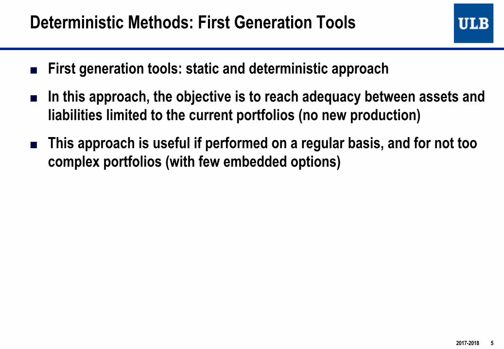
■ First generation tools: static and deterministic approach
■ In this approach, the objective is to reach adequacy between assets and liabilities limited to the current portfolios (no new production)
■ This approach is useful if performed on a regular basis, and for not too complex portfolios (with few embedded options)
Deterministic Methods: First Generation Tools
2017-2018 5

6
►Different analyses:● Measure of treasury gaps● Cash-flows matching● Duration, Convexity● Immunization
à Classical ALM methods from banking
Deterministic Methods: First Generation Tools
6ALM – Deterministic Methods 2017-2018

7
■ Purpose : Control of the asset – liability adequacy in terms of cash-flows● One of the purpose of ALM is to ensure a good adequacy between cash-
flows of the assets (e.g. coupon and notional payments of bonds) and cash-flows of the liabilities (claims)
● If cash-flow adequacy is very bad, the company is exposed among other to reinvestment and realisation risk
Measure of Treasury Gaps
7ALM – Deterministic Methods 2017-2018
8
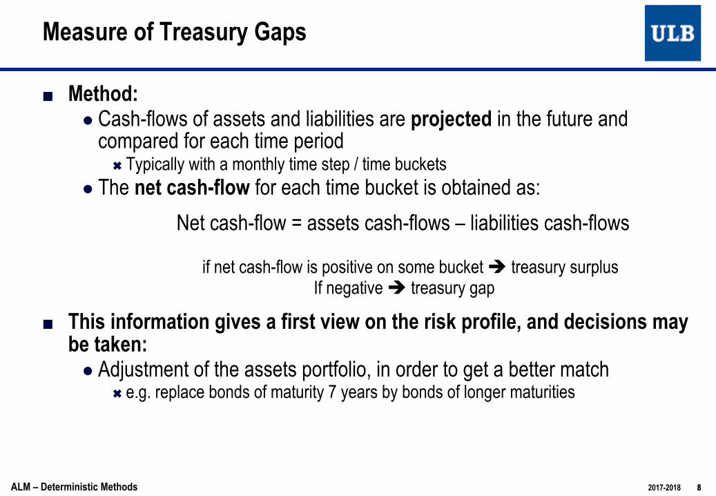
■ Method: ● Cash-flows of assets and liabilities are projected in the future and
compared for each time periodÓ Typically with a monthly time step / time buckets
● The net cash-flow for each time bucket is obtained as:
Net cash-flow = assets cash-flows – liabilities cash-flows
if net cash-flow is positive on some bucket è treasury surplus If negative è treasury gap
■ This information gives a first view on the risk profile, and decisions may be taken:
● Adjustment of the assets portfolio, in order to get a better match Ó e.g. replace bonds of maturity 7 years by bonds of longer maturities
Measure of Treasury Gaps
8ALM – Deterministic Methods 2017-2018

Measure of Treasury Gaps
2017-2018 9

10
■ Let us suppose that both assets and liabilities cash-flows are deterministic, not subject to financial markets nor policyholdersbehaviour
■ If for each period, the net cash-flow is positive, then the margin of the company is certain, independently of the evolution of financial markets
● No need for the company to go in the market for buying or selling assets, as liabilities cash-flows are exactly covered by assets cash-flows
■ In practice, cash-flows are not always deterministic (esp. for life insurance in presence of embedded options) and assumptions have to be taken (e.g. for surrender rates, see later)
■ This methodology can be useful to analyze liquidity risk, as most of stochastic models do not include explicitly this risk type
Measure of Treasury Gaps
10ALM – Deterministic Methods 2017-2018

11
■ General result: If liabilities cash-flows are deterministic, it is possible in theory to find a portfolio of fixed coupon bonds allowing to perfectlymatch these liabilities cash-flows (« cash-flow matching »)
■ Principle : construction of a portfolio of fixed coupons bonds such thatnet future cash-flows are zero, or at least positive
Cash-Flow Matching
2017-2018 11
Assets cash-flows
Liabilities cash-flows
time
ALM – Deterministic Methods

12
■ Let us consider an insurance portfolio with cash out-flows "# falling atdates {%&, … , %)}
■ Suppose that we can invest on the asset side in ) fixed coupons bonds, with maturity dates {%&, …, %)}, and coupons falling also within thesedates
■ We denote by +#(-) the cash in-flow of the jth bond at date %#
Methodology:
■ Select a fixed rate bond with maturity equal to the maturity of the last liabilities cash-flow (i.e. %))
■ Invest in this bond an amount such that the last cash-flow of that bond corresponds to the last liabilities cash-flowà quantity to buy: /) = ")
+)()) ,
Cash-Flow Matching
12ALM – Deterministic Methods 2017-2018

13
■ For the largest maturity, the liability cash-flow is perfectly matched on the asset side, but not for other (shorter) maturities
● We then need to know what are the remaining liability cash-flows for these maturities
àThe next step is to subtract from the liabilities, cash-flows falling at other maturities (the coupons paid) following the investment in this bond
àThe resulting cash-flows (after subtraction) have still to be “covered” by other bonds
● We then repeat the process for the penultimate liabilities cash-flow date !"#$, by considering these resulting cash-flows
■ This leads to solving a linear system in the unknown invested quantities%&,… , %) in bonds of maturities {+&, … , +)}
Cash-Flow Matching
13ALM – Deterministic Methods 2017-2018
14
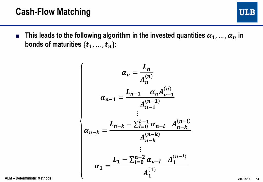
■ This leads to the following algorithm in the invested quantities !",… , !% in bonds of maturities {'", … , '%}:
!% =*%+%(%)
!%." =*%." − !%+%."%
+%."%."
⋮
!%.1 =*%.1 − ∑ !%.31."
345 +%.1%.3
+%.1%.1
⋮
!" =*" − ∑ !%.3%.7
345 +"%.3
+""
Cash-Flow Matching
14ALM – Deterministic Methods 2017-2018

15
Cash-Flows Matching : Example (1/3)
Gender Birth year monthly pension annual pension
H 1930 3600 43200F 1043 5400 64800F 1046 4600 55200H 1040 6700 80400F 1042 4250 51000H 1937 3800 45600H 1936 5200 62400H 1933 5800 69600F 1922 4300 51600F 1929 4500 54000
15ALM – Deterministic Methods 2017-2018
16
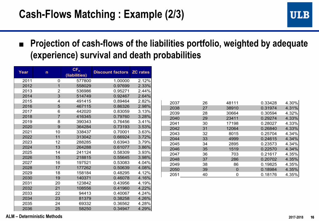
■ Projection of cash-flows of the liabilities portfolio, weighted by adequate (experience) survival and death probabilities
Cash-Flows Matching : Example (2/3)
Year n CFn
(liabilities)Discount factors ZC rates
2011 0 577800 1.00000 2.12%2012 1 558029 0.97699 2.33%2013 2 536986 0.95271 2.44%2014 3 514749 0.92467 2.64%2015 4 491415 0.89464 2.82%2016 5 467115 0.86326 2.98%2017 6 442020 0.83059 3.13%2018 7 416345 0.79760 3.28%2019 8 390343 0.76456 3.41%2020 9 364284 0.73193 3.53%2021 10 338437 0.70001 3.63%2022 11 313042 0.66924 3.72%2023 12 288285 0.63943 3.79%2024 13 264288 0.61077 3.86%2025 14 241124 0.58309 3.93%2026 15 218815 0.55645 3.98%2027 16 197521 0.53083 4.04%2028 17 177262 0.50639 4.08%2029 18 158184 0.48295 4.12%2030 19 140371 0.46078 4.16%2031 20 123842 0.43956 4.19%2032 21 108556 0.41960 4.22%2033 22 94413 0.40067 4.24%2034 23 81379 0.38258 4.26%2035 24 69332 0.36562 4.28%2036 25 58250 0.34947 4.29%
2037 26 48111 0.33428 4.30%2038 27 38910 0.31974 4.31%2039 28 30664 0.30594 4.32%2040 29 23411 0.29274 4.33%2041 30 17198 0.28027 4.33%2042 31 12064 0.26840 4.33%2043 32 8015 0.25704 4.34%2044 33 4999 0.24615 4.34%2045 34 2895 0.23573 4.34%2046 35 1519 0.22570 4.34%2047 36 703 0.21617 4.35%2048 37 286 0.20702 4.35%2049 38 86 0.19825 4.35%2050 39 0 0.18984 4.35%2051 40 0 0.18176 4.35%
16ALM – Deterministic Methods 2017-2018

17
■ Projection of cash-flows of the different bonds:
Cash-Flows Matching : Example (3/3)
17ALM – Deterministic Methods 2017-2018
n 1 2 3 4 5 6 7 8 9 10 11 12 13 14 15notional 100 100 100 100 100 100 100 100 100 100 100 100 100 100 100repayment at maturity 100 100 100 100 100 100 100 100 100 100 100 100 100 100 100coupon 2.20% 2.30% 2.50% 6.00% 3.00% 6.00% 3.30% 3.40% 3.45% 3.55% 3.58% 3.62% 3.68% 4.20% 4.30%
2011 Price -100 -100 -100 -100 -100 -100 -100 -100 -100 -100 -100 -100 -100 -100 -100 -15002012 102.20 2.30 2.50 6.00 3.00 6.00 3.30 3.40 3.45 3.55 3.58 3.62 3.68 4.20 4.30 155.082013 102.30 2.50 6.00 3.00 6.00 3.30 3.40 3.45 3.55 3.58 3.62 3.68 4.20 4.30 152.882014 102.50 6.00 3.00 6.00 3.30 3.40 3.45 3.55 3.58 3.62 3.68 4.20 4.30 150.582015 106.00 3.00 6.00 3.30 3.40 3.45 3.55 3.58 3.62 3.68 4.20 4.30 148.082016 103.00 6.00 3.30 3.40 3.45 3.55 3.58 3.62 3.68 4.20 4.30 142.082017 106.00 3.30 3.40 3.45 3.55 3.58 3.62 3.68 4.20 4.30 139.082018 103.30 3.40 3.45 3.55 3.58 3.62 3.68 4.20 4.30 133.082019 103.40 3.45 3.55 3.58 3.62 3.68 4.20 4.30 129.782020 103.45 3.55 3.58 3.62 3.68 4.20 4.30 126.382021 103.55 3.58 3.62 3.68 4.20 4.30 122.932022 103.58 3.62 3.68 4.20 4.30 119.382023 103.62 3.68 4.20 4.30 115.802024 103.68 4.20 4.30 112.182025 104.20 4.30 108.502026 104.30 104.30
3922.2 3798.1 3663.1 3521.3 3489.6 3343.3 3287.2 3135.6 2981.63 2826 2672.4 2520.6 2371.83 2227.5 2097.9number of bonds

18
■ It is not always possible to find bonds with a sufficiently good coincidence withCF dates of the liabilities. We then select bonds with payment dates as close as possible to these dates à small treasury gaps
■ For some bonds, coefficients (α) may be negative à treasury surplus if wecannot have short positions in bonds
■ We cannot always find bonds with a sufficiently long maturity with respect to the longest maturity of insurance contracts
● Need for buying in the future bonds not yet issued in the market
● Some uncertainty still remains
■ Outgoing cash-flows on the liability side are in practice only probable cash-flows (averaged with respect to mortality, reductions, surrender). These are not deterministic in practice
● In case of high volatility with respect to surrenders for instance, the methodology may be inefficient
Cash-flow Matching: Limitations
18ALM – Deterministic Methods 2017-2018

■ The second basic ALM technique is immunization, involving the concepts of duration and convexity
■ The duration is not a new concept since it was introduced in 1938 by Frederick Macaulay
■ The concept of duration can be appreciated at several levels:● It is a measure of the average life time of a fixed income product, in
particular of a fixed rate bond● It allows to measure the impact of a variation of interest rates on this
product● It eases the construction of investment strategies allowing to
neutralize positions in bonds (or more generally in interest rate sensitive products) against interest rate risk
Duration, convexity and immunization
1919ALM – Deterministic Methods 2017-2018

■ The computation of the duration consists in weighting the maturity of each flow by the proportion of the present value of this flow within the value of the FI product
■ The duration is thus different from the maturity of the product ● Maturity = point in time where the product holder will perceive the very last
cash flow
Duration: Definition
2020ALM – Deterministic Methods 2017-2018
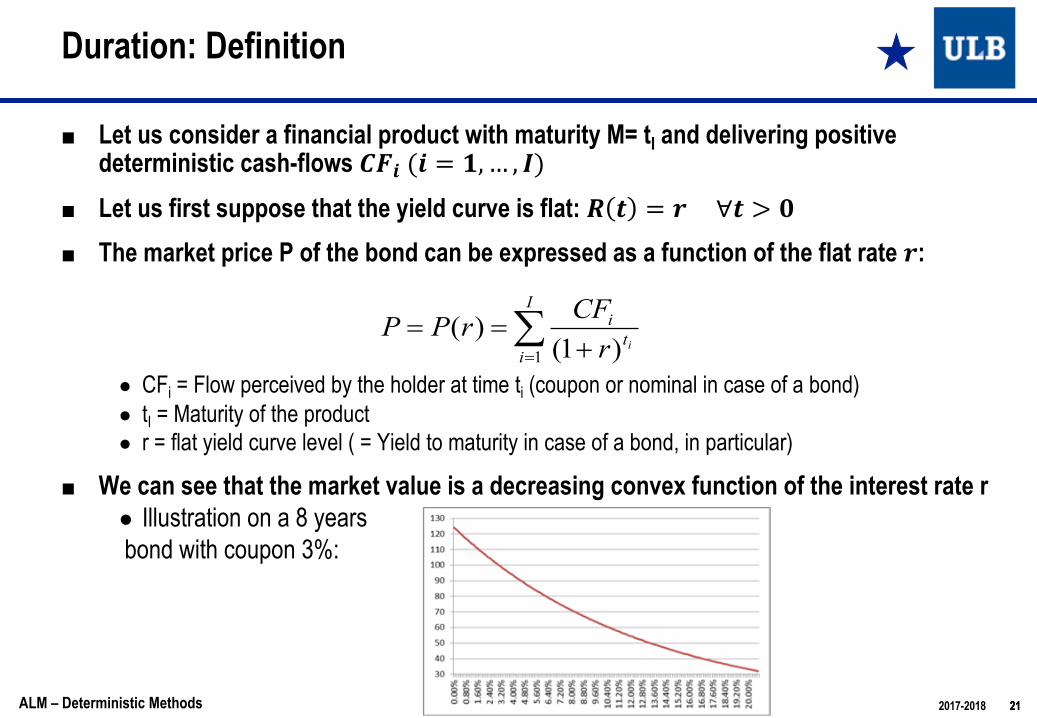
■ Let us consider a financial product with maturity M= tI and delivering positive deterministic cash-flows !"#(# = ',… , *)
■ Let us first suppose that the yield curve is flat: , - = .∀- > 1■ The market price P of the bond can be expressed as a function of the flat rate .:
● CFi = Flow perceived by the holder at time ti (coupon or nominal in case of a bond)● tI = Maturity of the product● r = flat yield curve level ( = Yield to maturity in case of a bond, in particular)
■ We can see that the market value is a decreasing convex function of the interest rate r● Illustration on a 8 yearsbond with coupon 3%:
Duration: Definition
å= +
==I
it
iir
CFrPP1 )1(
)(
2121ALM – Deterministic Methods 2017-2018

■ Clearly, an increase of the yield curve leads to a decrease of the market price of the product
● The first derivative w.r.t. !is indeed negative:
#$#% = −()*
+,*- + % )*/-
0
*1-≤ 3
(if all cash-flows 456 are assumed positive)
■ Positive convexity of the market value can be easily checked by computing the second derivative :
#7$#%7 =()*()* + -)
+,*- + % )*/7
0
*1-≥ 3
■ This positive convexity implies an asymmetry in the impact of interest rates movements: ● The market value will increase more for a 1% decrease of interest rates than it will
decrease for a 1% increase of rates
Duration: Definition
2222ALM – Deterministic Methods 2017-2018

■ Effect of positive convexity:
Duration: Definition
2017-2018 23
r*
P*
Price
Yield
Market price curve
Tangent (slope = 1st derivative)

■ Let us suppose that the (flat) yield curve makes a shift to the value ! + #$■ By decomposing the product market price in Taylor series around the current
yield curve level, the price variation for a variation of the interest rates can be decomposed in:
■ Clearly, for a given interest rates movement #$, ● The higher the first derivative, the higher the impact on the market price of the
product● The higher the second derivative, the higher the asymmetry between the positive
impact in case of rates decrease and the negative impact in case of rates increase
Duration: Definition
2424ALM – Deterministic Methods 2017-2018
2)()()(
²)(2
)()()()()()(
2
2
2
2
2
2
rdrrPd
rdrrdP
ror
drrPd
rdrrdP
rPrrPrP
D+D@
D+D
+D=-D+=D

■ Even if the yield curve is non flat, we can express the market price of a fixed income product as a function of a unique rate, its yield to maturity:
● CFi = Flow perceived by the holder at time ti (coupon or nominal in case of a bond)● tn = Maturity● r = Yield to maturity (of the bond, derived from the market price of that bond)
■ Taylor expansion of the price in function now of the yield to maturity becomes:
Duration: Definition
å= +
==n
it
iir
CFrPP1 )1(
)(
²)(2
)()()()()(2
2
2
ror
drrPd
rdrrdP
rPrrPrP D+D
+D=-D+=D
2525ALM – Deterministic Methods 2017-2018
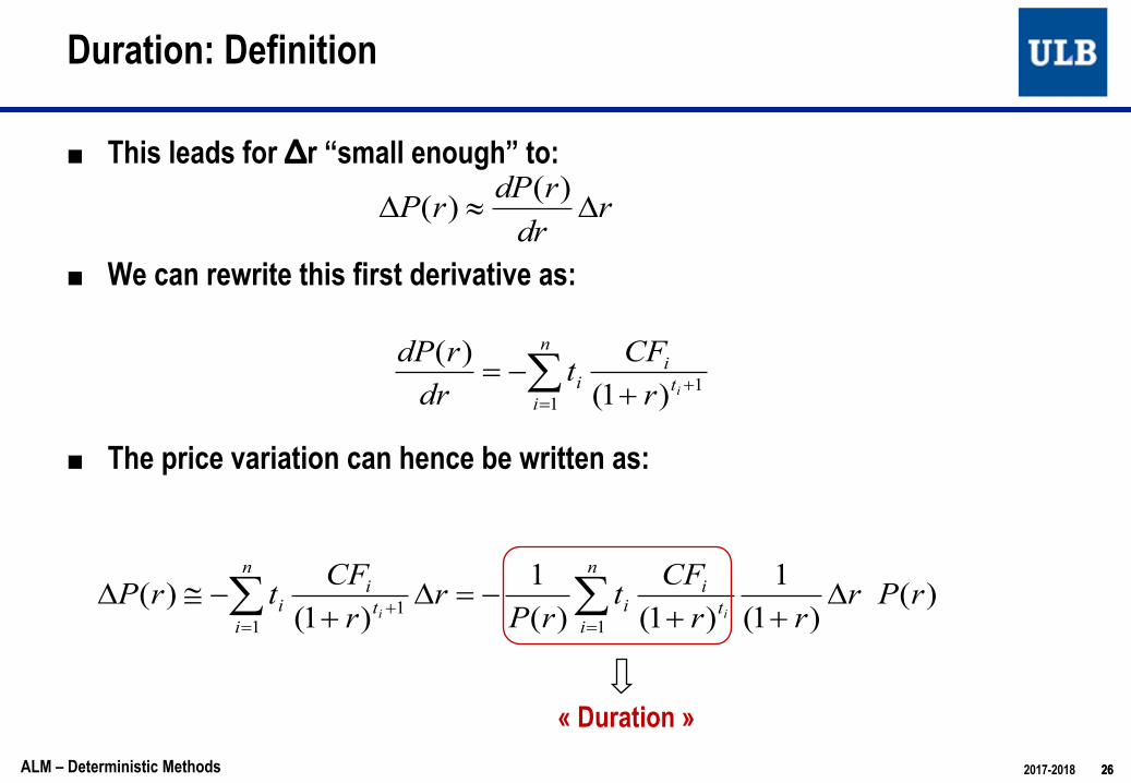
■ This leads for Δr “small enough” to:
■ We can rewrite this first derivative as:
■ The price variation can hence be written as:
Duration: Definition
rdrrdPrP D»D)()(
11 )1(
)(+
= +-= å it
in
ii rCFt
drrdP
2626ALM – Deterministic Methods 2017-2018
)( )1(
1)1()(
1)1(
)(1
11
rPrrr
CFtrP
rrCFtrP
ii ti
n
iit
in
ii D
++-=D
+-@D åå
=+
=
« Duration »

■ The (Macaulay) duration D is defined by the following formula:
■ We can hence rewrite the price variation as:
■ The price variation of the product (e.g. fixed rate bond) is proportional to the variation of the (flat) yield curve rate (or generally of its yield to maturity), with proportionality factor –D/(1+r)
● This new factor, D/(1+r), will be called “modified duration”
Duration: Definition
úû
ùêë
é+
= å=
n
itiiir
CFtP
D1 )1(.1
,
)1(
)1(
1
1
å
å
=
=
+
+=Û n
it
i
n
it
ii
i
i
rCFr
CFtD
27
rrPr
DrP D+
-»D )(11)(
27ALM – Deterministic Methods 2017-2018

■ The duration appears like an average maturity, since it is equal to the weighted average of the payment instants ti weighted by the discounted cash-flows
● The higher the discounted value* of the cash-flow !"# in the market value, the higher the weight given to the instant $# in the duration
■ Highlighting of the weighting coefficients:
where weighting coefficients are:
à kind of “first moment”
* Discounted with the YTM in case of non flat yield curve
Duration: Interpretation
å=
=n
iii twD
1.
iti
i rCF
Pw
)1(1
+´=
2828ALM – Deterministic Methods 2017-2018

■ Let us first suppose that the yield curve is flat at the level ! = #. %&%■ Computation of the duration of a 4-year bond with a nominal of EUR
1000, paying annual coupons of 3%
● Step 1: Computation of the bond price (denominator)
Duration: Example
Year Flat yield curve Discount factor Cash-Flow Discounted CF
1
3.25%
0.968523 30 29.06
2 0.938037 30 28.14
3 0.908510 30 27.26
4 0.879913 1030 906.31
TOTAL 990.76
= 1/(1+3.25%)1
2929ALM – Deterministic Methods 2017-2018
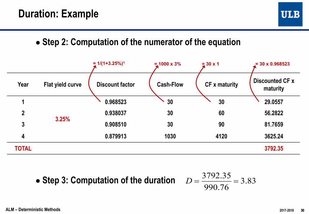
● Step 2: Computation of the numerator of the equation
● Step 3: Computation of the duration
Duration: Example
Year Flat yield curve Discount factor Cash-Flow CF x maturity Discounted CF x maturity
1
3.25%
0.968523 30 30 29.0557
2 0.938037 30 60 56.2822
3 0.908510 30 90 81.7659
4 0.879913 1030 4120 3625.24
TOTAL 3792.35
= 1/(1+3.25%)1 = 30 x 1 = 30 x 0.968523= 1000 x 3%
83.376.99035.3792
==D
3030ALM – Deterministic Methods 2017-2018

■ Let us now consider a 4-year bond with nominal EUR 1000, but paying annual coupons of 10%.
● Step 1: Computation of the bond price (denominator)
Duration: Example
Year Flat yield curve Discount factor Cash-Flow Discounted CF
1
3.25%
0.968523 100 96.85
2 0.938037 100 93.80
3 0.908510 100 90.85
4 0.879913 1100 967.90
TOTAL 1249.41
= 1/(1+3.25%)1
3131ALM – Deterministic Methods 2017-2018

● Step 2: Computation of the numerator of the equation
● Step 3: Computation of the duration
Duration: Example
Year Flat yield curve Discount factor Cash-Flow CF x maturity Discounted CF x maturity
1
3.25%
0.968523 100 100 96.85
2 0.938037 100 200 187.61
3 0.908510 100 300 272.55
4 0.879913 1100 4400 3871.62
TOTAL 4428.63
= 1/(1+3.25%)1 = 30 x 1 = 30 x 0.968523= 1000 x 3%
54.341.124963.4428
==D
3232ALM – Deterministic Methods 2017-2018

■ Duration of bond 1 is 3.83 while duration of bond 2 is 3.54
■ Those two bonds have the same maturities, but bond 2 has a shorter duration
■ This is not surprising if we think in terms of duration as a weighted average of instants of cash-flow payments:
● There are more cash-flows paid by bond nr.2 before maturity, hence these cash-flows will give more weight to instants smaller than the maturity of the bond, leading to a smaller duration
Duration: Example
3333ALM – Deterministic Methods 2017-2018

■ Computation is the same as before, except that the level of the flat yield curve (which is not flat anymore) is replaced by the yield to maturity of the bond
● In the case of bond 1, calculations remain identical once we know the YTM of the bond. In the current case, this YTM is 3.46%
● Step 1: Computation of the bond price (denominator)
Duration: Example in case of non flat yield curve
Year Yieldcurve
Yield to maturity
« Discount factor » (from YTM) Cash-Flow Discounted
CF
1 2.0%
3.46%
0.966536 30 29.00
2.5%2 0.934192 30 28.03
3 0.902930 30 27.093%
4 0.872715 1030 898.903.5%
TOTAL 983.01
= 1/(1+3.46%)1
3434ALM – Deterministic Methods 2017-2018
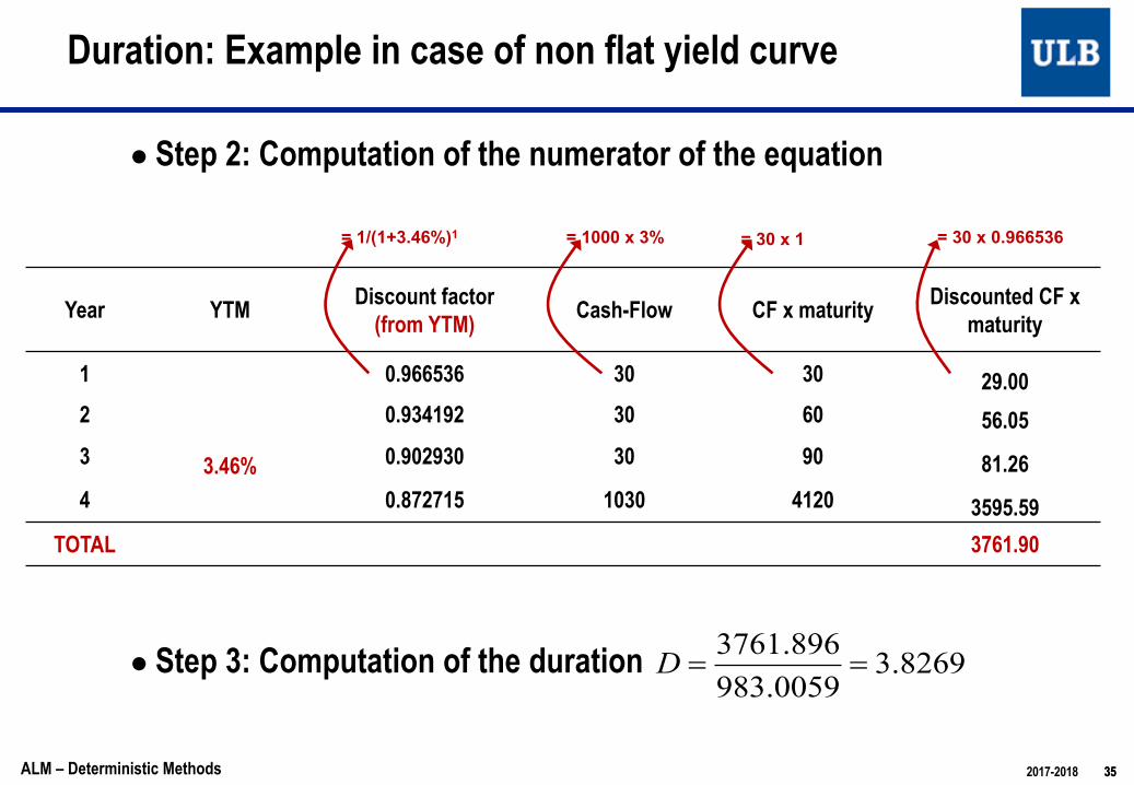
● Step 2: Computation of the numerator of the equation
● Step 3: Computation of the duration
Duration: Example in case of non flat yield curve
Year YTM Discount factor(from YTM) Cash-Flow CF x maturity Discounted CF x
maturity
1
3.46%
0.966536 30 30 29.002 0.934192 30 60 56.053 0.902930 30 90 81.264 0.872715 1030 4120 3595.59
TOTAL 3761.90
= 1/(1+3.46%)1 = 30 x 1 = 30 x 0.966536= 1000 x 3%
8269.30059.983896.3761
==D
3535ALM – Deterministic Methods 2017-2018

■ The bond price is sensitive to variations of interest rates in the market
■ This sensitivity can be measured with “some” precision thanks to the duration
■ Hopewell and Kaufman proposed in 1973 a definition of the duration by calculating the derivative of the bond price as a function of its yield to maturity (cf. definition introduced here)
Duration and Sensitivity
3636ALM – Deterministic Methods 2017-2018

■ Expressed in another way, the relative variation of the bond price P for a given variation !" of its yield r is equal to:
■ This new factor “Duration / (1 + Yield to Maturity)” is defined as the modified duration (Dm) , also called product sensitivity
■ It represents the percentage of variation of the bond price for a variation of 1% of its yield to maturity
■ More generally, in terms of present value of a product (or position) with deterministic cash-flows, we can write:
Modified Duration
rD
PrP
+-@
DD
11
rrPVDrPV m D-»D )()(
(1)37
(1)
ALM – Deterministic Methods 2017-2018
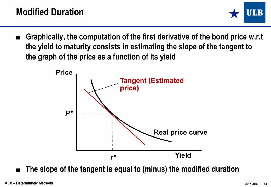
■ Graphically, the computation of the first derivative of the bond price w.r.t the yield to maturity consists in estimating the slope of the tangent to the graph of the price as a function of its yield
■ The slope of the tangent is equal to (minus) the modified duration
Modified Duration
r*
P*
Price
Yield
Real price curve
Tangent (Estimatedprice)
3838ALM – Deterministic Methods 2017-2018

■ Modified duration gives an approximation of the relative variation of the price that is appropriate for small variations of its yield around r* , but that becomes more and more imperfect for larger yield changes
● The modified duration underestimates the increase of the bond price in case of decrease of its yield● The modified duration overestimates the decrease of the bond price in case of increase of its yield● The duration must thus be completed by the convexity, involving the second derivative
Modified Duration
Underestimation of the increase
Overestimation of the decrease
r*
P*
3939ALM – Deterministic Methods 2017-2018

■ Duration of a zero-coupon bond● We easily see that for a zero-coupon bond, Duration = Time to Maturity
Ó NB: This is the only case for which the realized yield at maturity is already known at the acquisition date: there is no risk of reinvestment of the coupons
■ Duration of a product with positive cash-flows● We can see that the proportionality factor in equation (1) (slide 37) is
always negative● Sensitivity of such a product is always negative● The duration is always positive● This is the case of bonds in particular
Duration in specific cases
40ALM – Deterministic Methods 2017-2018
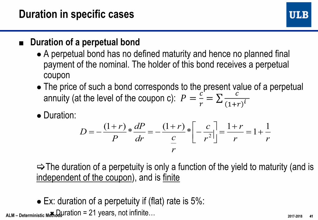
■ Duration of a perpetual bond● A perpetual bond has no defined maturity and hence no planned final
payment of the nominal. The holder of this bond receives a perpetual coupon
● The price of such a bond corresponds to the present value of a perpetual annuity (at the level of the coupon c): ! = #
$ = ∑ #&'$ (
● Duration:
[The duration of a perpetuity is only a function of the yield to maturity (and is independent of the coupon), and is finite
● Ex: duration of a perpetuity if (flat) rate is 5%: Ó Duration = 21 years, not infinite…
Duration in specific cases
rrr
rc
rcr
drdP
PrD 111*)1(*)1(
2 +=+
=úûù
êëé-
+-=
+-=
4141ALM – Deterministic Methods 2017-2018
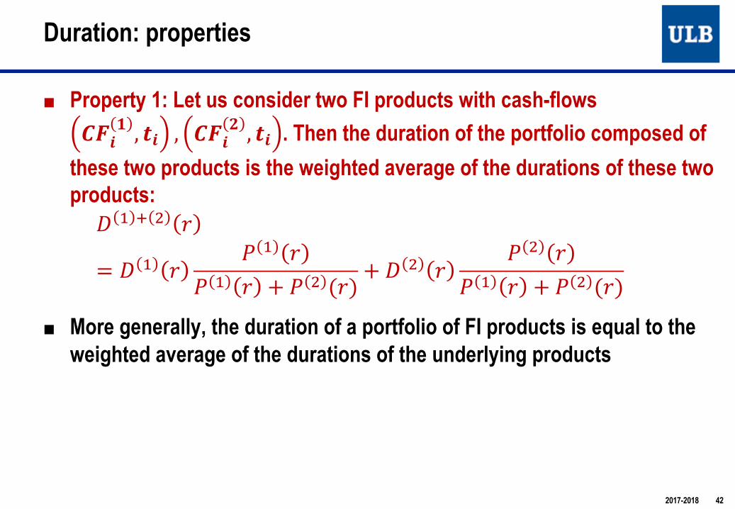
■ Property 1: Let us consider two FI products with cash-flows !"#$ , &# , !"#' , &# . Then the duration of the portfolio composed of
these two products is the weighted average of the durations of these twoproducts: ( ) * + ,= ( ) , . ) ,
. ) , + . + (,) + (+ , . + ,
. ) , + . + (,)■ More generally, the duration of a portfolio of FI products is equal to the
weighted average of the durations of the underlying products
Duration: properties
2017-2018 42

■ Property 2: Let us consider a FI product with cash-flows !"#$ , &# and let ' be a constant. Then the duration of a product delivering cash-flows ' ∗ !"#$ , &# is equal to the duration of the initial product
)'∗ $ * = ) $ (*)
Duration: properties
2017-2018 43

■ Let us consider a FI product with positive cash-flows !"# , %# and let us consider its duration as a function of (current) time and rate (or YTM) : & = &%())
■ Property 3: &% ) = &+ ) − %(duration increases linearly with time)
■ Property 4: Duration is a decreasing function of the interest rate (or YTM) and its derivative w.r.t. )is given by:
.&%()).) = − /
/ + )12
where 12 = ∑ %#24#5#6/ − ∑ %#4#
5#6/ 2 ≥ +, and 4# =
!"#/8) %#9())
Duration: properties
2017-2018 44

45
■ If (Dr)2 is sufficiently small,
■ Now,
■ We define the convexity by:
Convexity: definition
2)()()()(2
2
2 rdr
rPVdrdrrdPVrPV D
+D»D
21
2
2
)1()1()(
+= +
+=å i
i
tt
n
iii r
CFtt
drrPVd
å
å
=
=
+
++
= n
it
t
n
it
tii
i
i
i
i
rCF
rCF
ttQ
1
1
)1(
)1()1(
45ALM – Deterministic Methods 2017-2018

46
■ We can rewrite convexity as:
■ Convexity can be seen as the sum of first and second (non centered) moments of a random variable T taking values !" with probability #"(which belong to [0,1] as cash-flows are assumed positive)
Convexity: interpretation
å ååå
å= ==
=
= +=+=
+
++
=n
i
n
iiiii
n
iiiin
it
t
n
it
tii
wtwtwtt
rCF
rCF
ttQ
i
i
i
i
1 1
2
1
1
1 )1(
)1(
)1()1(
46ALM – Deterministic Methods 2017-2018
Duration

47
■ We can continue the interpretation:
■ The last term !" corresponds to the variance of that random variable T, and is hence a measure of the « dispersion » of the cash-flows aroundthe duration
■ Hence, for a given duration, the higher the dispersion of the cash-flows, the higher the convexity
● Rem: we have seen previously that #$%(')#' = − +
+,' !"
Convexity: interpretation
47ALM – Deterministic Methods 2017-2018
22
22
222
2
1 1
2
]])[[(])[(][])[(])[(][][
][][
VDDTETETETETETETETE
TETEwtwtQn
i
n
iiiii
++=
-++=
-++=
+=+=å å= =

■ Let us consider a bond with coupon 4% and maturity 10 year
■ Yield curve is flat at 3%
● Duration: 8.51
● Dispersion V² : !"#.#%&"!.'% = ). *%● Convexity: D + D² + V² = 88.34
Convexity: example
2017-2018 48
T_i DF CF PV CF t xPV CF t² x PV CF (t-D)² x PV CF1 0.970873786 4 3.88 3.88 3.88 218.952 0.942595909 4 3.77 7.54 15.08 159.723 0.915141659 4 3.66 10.98 32.95 111.084 0.888487048 4 3.55 14.22 56.86 72.255 0.862608784 4 3.45 17.25 86.26 42.486 0.837484257 4 3.35 20.10 120.60 21.087 0.813091511 4 3.25 22.77 159.37 7.408 0.789409234 4 3.16 25.26 202.09 0.829 0.766416732 4 3.07 27.59 248.32 0.7410 0.744093915 104 77.39 773.86 7738.58 172.11
total 108.53 923.45 8663.98 806.63

■ Let us now consider a 10 years bond with a 20% coupon (same flat YC)
● Duration: 6.69 à smaller duration
● Dispersion V² : !"#$!%" = '(. %*à higher dispersion
● Convexity: D + D² + V² = 62.03 à smaller convexity
■ This second bond has a smaller convexity although dispersion is higher, and this is due to itssmaller duration
■ Hence convexity is not equivalent to dispersion
Convexity: example
2017-2018 49
T_i DF CF PV CF T xPV CF t² x PV CF (t-D)² x PV CF1 0.970873786 20 19.42 19.42 19.42 630.232 0.942595909 20 18.85 37.70 75.41 415.923 0.915141659 20 18.30 54.91 164.73 250.174 0.888487048 20 17.77 71.08 284.32 129.265 0.862608784 20 17.25 86.26 431.30 49.696 0.837484257 20 16.75 100.50 602.99 8.147 0.813091511 20 16.26 113.83 796.83 1.498 0.789409234 20 15.79 126.31 1010.44 26.809 0.766416732 20 15.33 137.96 1241.60 81.2910 0.744093915 120 89.29 892.91 8929.13 974.11
total 245.01 1640.87 13556.16 2567.10

■ Property 1: Let us consider two FI products with cash-flows !"#$ , &# , !"#' , &# . Then the convexity of the portfolio composed
of these two products is the weighted average of the convexities of these two products:
( ) * + ,= ( ) , . ) ,
. ) , +. + (,) + (+ , . + ,
. ) , +. + (,)
■ More generally, the convexity of a portfolio of FI products is equal to the weighted average of the convexities of the underlying products
Convexity: properties
2017-2018 50

■ Property 2: Let us consider a FI product with cash-flows !"#$ , &# and let ' be a constant. Then the convexity of a product delivering cash-flows ' ∗ !"#$ , &# is equal to the convexity of the initial product
)'∗ $ * = ) $ (*)
Convexity: properties
2017-2018 51

52
■ We can then use duration and convexity to get the approximation:
■ à Always positive impact of convexity
à « more convexity is better »
This is because: ● A rate decrease results in a higher increase of the FI product if its
convexity if higher, for a given level of duration● A rate increase results in a smaller decrease of the product if its convexity
is higher, for a given level of duration
Convexity and sensitivity
)()2)(
)1(1
11()(
2
2 rPVrr
Qrr
DrPV D+
+D+
-»D
52ALM – Deterministic Methods 2017-2018

53
■ Bond with time to maturity 5 years, annual coupon of 5, nominal of 100
■ Yield to maturity (or flat yield curve is) : 7%
■ Price =91.79961, Duration=4.52, Convexity=26.22
■ Increase of rates : (YTM=9%)● Price (Exact calculation)=84.44139● Price (Approx, order 1)=84.03835● Price (Approx, order 2)=84.45877
■ Decrease of rates : (YTM=5%)● Price (Exact calculation)=100● Price (Approx, order 1)=99.56086● Price (Approx, order 2)=99.98129
Approximation of a Price Variation by Duration and Convexity Example
53ALM – Deterministic Methods 2017-2018
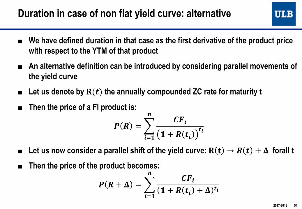
■ We have defined duration in that case as the first derivative of the product pricewith respect to the YTM of that product
■ An alternative definition can be introduced by considering parallel movements of the yield curve
■ Let us denote by !(#) the annually compounded ZC rate for maturity t
■ Then the price of a FI product is:
% & =( )*+, + & #+
#+
.
+/,
■ Let us now consider a parallel shift of the yield curve: ! 0 → & # + 2 forall t
■ Then the price of the product becomes:
% & + 2 =( )*+, + & #+ + 2 #+
.
+/,
Duration in case of non flat yield curve: alternative
2017-2018 54

■ The first derivative of the price w.r.t. ! is given by:"# $ + !
"! &!'(
= −+,-./-
0 + $ ,-,-10
2
-'0
■ This cannot be rewritten in terms of weighted average of instants of payments involving discounted values of the CFs
■ We will consider instead continuously compounded rates
Duration in case of non flat yield curve : alternative
2017-2018 55
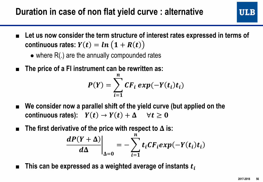
■ Let us now consider the term structure of interest rates expressed in terms of continuous rates: ! " = $% ' + ) "
● where R(.) are the annually compounded rates
■ The price of a FI instrument can be rewritten as:
* ! =+,-./01(−! ". ".)%
.5'
■ We consider now a parallel shift of the yield curve (but applied on the continuous rates): ! " → ! " + 7∀" ≥ :
■ The first derivative of the price with respect to 7is:;* ! + 7
;7 <75:
= −+".,-./01 −! ". ".%
.5'
■ This can be expressed as a weighted average of instants ".
Duration in case of non flat yield curve : alternative
2017-2018 56

■ By defining the duration !" as:
!" = ∑ %&'(&)*+ %& %&,&-.
/(+)we again obtain:
2/ + + 424 5
4-6= −!" ∗ /
Once again, duration can be seen as an average time (weighted by the discounted CFs):
!" =9%&:&
,
&-.
where :& = '(&);+ %& %&∑ '(&);+ %& %&,&<.
(w> ∈ 6, . if positive CFs)
Duration in case of non flat yield curve : alternative
2017-2018 57

■ We can again define convexity (from the second derivative) as follows:
!" = ∑ %&'()&*+, %& %&-&./
0(,)And we obtain:
3'0 , + 535' 6
5.7= !" ∗ 0
Once again, convexity can be seen as a non-centered second moment:
!" =9%&':&
-
&./= ; <' = ; < ' + ; < − ; < ' = >"' + ?"'
:& =()&*+, %& %&
∑ ()&*+, %& %&-&./
∈ [7, /]
Convexity in case of non flat yield curve : alternative
2017-2018 58
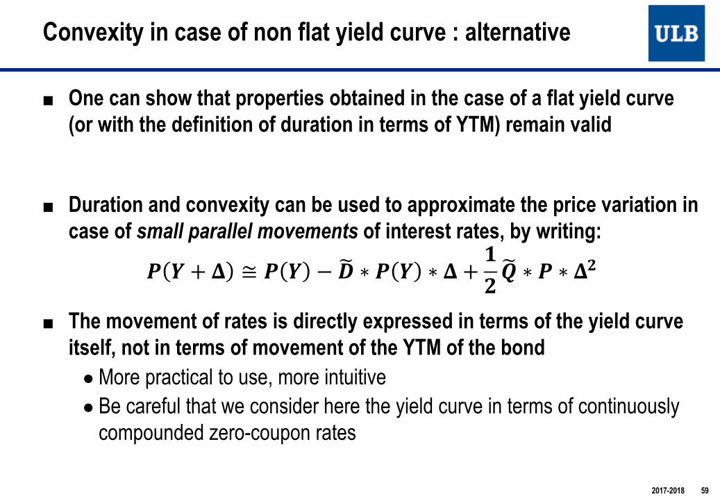
■ One can show that properties obtained in the case of a flat yield curve(or with the definition of duration in terms of YTM) remain valid
■ Duration and convexity can be used to approximate the price variation in case of small parallel movements of interest rates, by writing:
! " + $ ≅ ! " − '( ∗ ! " ∗ $ + *+,( ∗ ! ∗ $+
■ The movement of rates is directly expressed in terms of the yield curveitself, not in terms of movement of the YTM of the bond
● More practical to use, more intuitive● Be careful that we consider here the yield curve in terms of continuously
compounded zero-coupon rates
Convexity in case of non flat yield curve : alternative
2017-2018 59
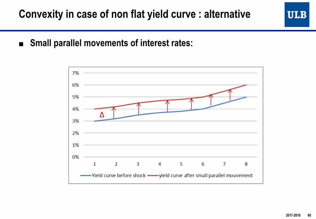
■ Small parallel movements of interest rates:
Convexity in case of non flat yield curve : alternative
2017-2018 60

■ Example
■ Price: 93.77
■ Duration: 6.93
■ Dispersion: 4.35
■ Convexity: 52.33
Convexity in case of non flat yield curve : alternative
2017-2018 61
Times Y(t) DF CF PV CF t x PV CF(t-D)² x PV
CF1 3% 0.970446 4 3.881782 3.881782 136.36012 3.20% 0.938005 4 3.75202 7.50404 91.078083 3.50% 0.900325 4 3.601298 10.80389 55.534174 3.70% 0.862431 4 3.449724 13.7989 29.553045 3.80% 0.826959 4 3.307837 16.53918 12.28196 4% 0.786628 4 3.146511 18.87907 2.7033457 4.50% 0.729789 4 2.919155 20.43409 0.0155968 5% 0.67032 104 69.71328 557.7063 80.27686
93.77161 649.5472 407.8031
This is done to compute the dispersion V²
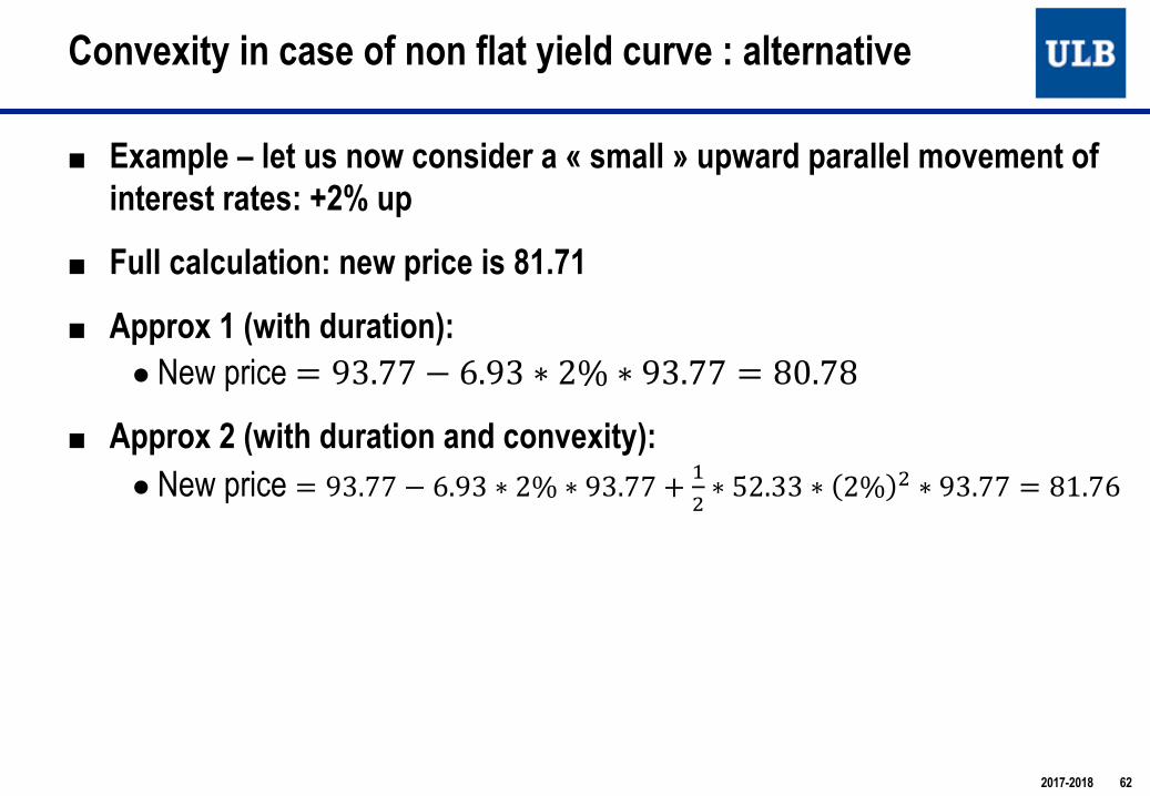
■ Example – let us now consider a « small » upward parallel movement of interest rates: +2% up
■ Full calculation: new price is 81.71
■ Approx 1 (with duration): ● New price = 93.77 − 6.93 ∗ 2% ∗ 93.77 = 80.78
■ Approx 2 (with duration and convexity):● New price = 93.77 − 6.93 ∗ 2% ∗ 93.77 + .
/ ∗ 52.33 ∗ 2% / ∗ 93.77 = 81.76
Convexity in case of non flat yield curve : alternative
2017-2018 62
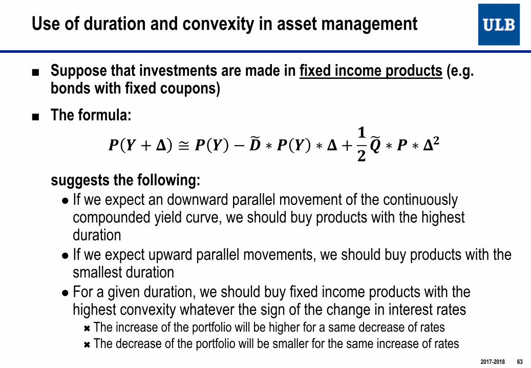
■ Suppose that investments are made in fixed income products (e.g. bonds with fixed coupons)
■ The formula:
! " + $ ≅ ! " − '( ∗ ! " ∗ $ + *+,( ∗ ! ∗ $+
suggests the following:● If we expect an downward parallel movement of the continuously
compounded yield curve, we should buy products with the highestduration
● If we expect upward parallel movements, we should buy products with the smallest duration
● For a given duration, we should buy fixed income products with the highest convexity whatever the sign of the change in interest rates
Ó The increase of the portfolio will be higher for a same decrease of ratesÓ The decrease of the portfolio will be smaller for the same increase of rates
Use of duration and convexity in asset management
2017-2018 63

■ Example● Suppose we can invest in two bonds of same coupon but different
maturitiesÓ Bond 1: coupon 4%, maturity 8 yearsÓ Bond 2: coupon 4%, maturity 5 yearsÓ Yield curve as in the previous example:
● Bond 1: Ó Price:93.77, Duration: 6.93, dispersion: 4.35, convexity: 52.33
● Bond 2: Ó Price: 100.69 , Duration: 4.63, dispersion: 0.99, convexity: 22.41
Use of duration and convexity in asset management
2017-2018 64

■ Example● Suppose the yield curve decreases by 1%● Impact on bond 1:
Ó New price is 100.52, hence an increase of 7.2%● Impact on bond 2:
Ó New price is 105.46, hence an increase of 4.7%● The impact on bond 2 is smaller due to its smaller duration
Ó Duration bond 1 was 6.93, duration bond 2 was 4.63Ó Remark that durations have slightly moved with the movement of interest rates as
well¦ New duration bond 1: 6.97¦ New duration bond 2: 4.64
Use of duration and convexity in asset management
2017-2018 65

■ Example● Let us consider now a zero-coupon bond of maturity 6.93
Ó Duration: 6.93, dispersion: 0, convexity : 6.93% = 47.98Ó This bond has the same duration as bond 1, but its convexity is smallerÓ Price: 73.39 (corresponding to a ZC rate for maturity 6.93 of 4.465%, obtained by
linear interpolation on rates, and for a notional of 100)
● Let us suppose as above that rates move downwards by 1% ● Impact on bond 1:
Ó New price is 100.52, hence an increase of 7.20%● Impact on the ZC bond:
Ó New price: 78.66, hence an increase of 7.17%● The price increase of the ZC bond is slightly smaller than for bond 1 due
to its smaller dispersion (and hence smaller convexity)Ó The difference is however very tiny (!), as duration is the most important factor in the
increase (order 1 w.r.t. order 2 effect)
Use of duration and convexity in asset management
2017-2018 66
67
■ Duration and convexity are well adapted to products with deterministiccash-flows, independent of the evolution of interest rates in the market
■ In the case of insurance contracts with few optionalities, and a guaranteed rate, liabilities cash-flows can be seen as independent of interest rates
● Remark that this is not necessarily the case, as insurance contracts have in general variable cash-flows due to embedded options
Ó Profit sharing, surrenders, reductions, more complex financial guarantees, …
■ Duration is then computed as for FI products
Duration in ALM: Duration of Insurance Contracts
2017-2018 67ALM – Deterministic Methods

68
■ Principle : we impose equality between the (first order) sensitivity of assets and liabilities
■ Suppose that we can cover insurance liabilities by fixed coupons bonds on the asset side
■ We want to find the quantities α1…αn of bonds to buy in order to have immunisation, i.e. duration(assets) = duration(liabilities):
■ We can also consider convexity, and impose positive convexity of the surplus:
Convexity(assets) ≥ Convexity(liabilities)
Immunisation
and 1
sliabilitie
n
iasseti PVPV
i=å
=
a
sLiabilitie
iasseti
iiasseti
sLiabilitieAssets
sliabilitien
i
asseti
DP
DPDD
drPVd
drPd
i
i
i
=Û=Û
=
å
å
å=
a
a
a
)()(
1
68ALM – Deterministic Methods 2017-2018

■ In summary, the standard immunisation condition for an insurancesegment can hence be summarized as follows:
69
PV of assets = PV of liabilitiesDuration of assets = Duration of liabilitiesConvexity of assets ≥ Convexity of liabilities
Immunisation
69ALM – Deterministic Methods 2017-2018

70
■ Portfolio of Insurance contracts with 2 maturities: 4 and 8 years.
■ Technical provisions of each sub-portfolio: € 5 Mio .
■ Hyp: No surrender, probable cash-flows (w.r.t. mortality) are projected
■ PV of liabilities : € 9.72 Mio
■ Duration of liabilities = 6 years.
■ On the assets side, we can choose between 2 portfolios
Immunisation: Simple Example
First Portfolio Market price DurationBond at 5.25% 99.1 3.71Bond at 5.75% 101.9 7.90
Second Portfolio Market price DurationBond at 5% 99.1 1.91Bond at 6% 104.3 8.96
70ALM – Deterministic Methods 2017-2018

71
■ Investment in first portfolio:● Duration = 3.71&' + 7.9&* = 6 (&- = proportion invested in bond i)● &' + &* = 1● à &' = 0.45, &* = 0.55● è a1 = 0.45*9.72 Mio / 99.1 = 44477, a2 = 52133 (# of bonds)
■ Investment in second portfolio:● Same reasoning è a3 = 41181, a4 = 54065
■ But: Convexity of the second portfolio is more important (exercice)● Dispersion in time of cash-flows is more important ● A priori, this second solution is preferred if we want to maximize convexity
of the surplus
Immunisation: Simple Example
71ALM – Deterministic Methods 2017-2018

72
■ Duration can be used as a first approximation of the assets or liabilitiesPV variation for small parallel movements of interest rates
● As only the first derivative is used● For greater movements, the second derivative should be considered à
convexity
■ Duration is only defined for fixed income products● In case of a stochastic cash-flows, also depending on interest rates, the
notion can be useful but the definition should be adapted
■ Duration makes few sense in the case of stocks or real estate● Duration is a tool defined for fixed income products!
■ Duration of a portfolio: ● Calculate first the duration of each security● Calculate then the weighted average of these durations, weighted by PV
of the securities
Duration : First Limitations
72ALM – Deterministic Methods 2017-2018

73
■ Duration and convexity are well adapted to products with deterministiccash-flows, independent of the evolution of interest rates in the market
● Now, insurance contracts have in general variable cash-flows due to embedded options
Ó Profit sharing, surrenders, reductions, more complex financial guarantees, … ● An average (or best estimate) duration can be calculated by projecting
probable cash-flows under best estimate hypotheses for these embeddedoptions
● Upper and lower bounds for the duration can also be calculated
■ Possibility to perform a scenario analysis related to the exercise of these embedded options
● We then calculate the duration under different scenarios or hypotheses related to embedded options
Duration of Insurance Contracts (1/5)
2017-2018 73ALM – Deterministic Methods

74
■ Example● Capital paid after 10 years (capitalisation bonds)● Guaranteed rate of 5%, unique premium● Hypothesis for the surrender option : between 5% and 15% per year● We project cash-flows of insurance contracts under these two extreme
hypotheses. The duration can hence be upper and lower bounded
Duration of Insurance Contracts (2/5)
74ALM – Deterministic Methods 2017-2018
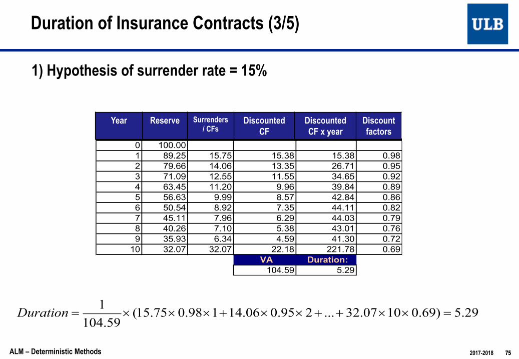
75
1) Hypothesis of surrender rate = 15%
Duration of Insurance Contracts (3/5)
2017-2018 75
Année
Provision math
rachats cash-flows actualisés
cash-flows actualisés x
année DF
0 100.001 89.25 15.75 15.38 15.38 0.982 79.66 14.06 13.35 26.71 0.953 71.09 12.55 11.55 34.65 0.924 63.45 11.20 9.96 39.84 0.895 56.63 9.99 8.57 42.84 0.866 50.54 8.92 7.35 44.11 0.827 45.11 7.96 6.29 44.03 0.798 40.26 7.10 5.38 43.01 0.769 35.93 6.34 4.59 41.30 0.7210 32.07 32.07 22.18 221.78 0.69
VA Duration: 104.59 5.29
29.5)69.01007.32...295.006.14198.075.15(59.1041
=´´++´´+´´´=Duration
Year Reserve Surrenders/ CFs
DiscountedCF
DiscountedCF x year
Discount factors
ALM – Deterministic Methods
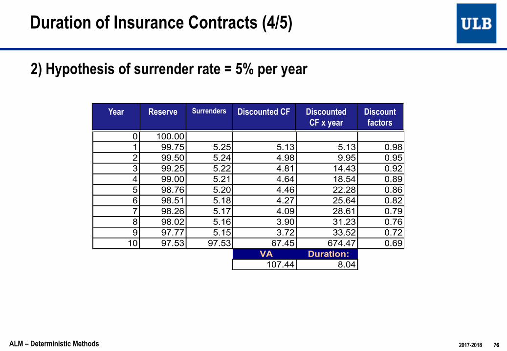
76
2) Hypothesis of surrender rate = 5% per year
Duration of Insurance Contracts (4/5)
2017-2018 76
Année
Provision math
rachats cash-flows actualisés
cash-flows actualisés x
année DF
0 100.001 99.75 5.25 5.13 5.13 0.982 99.50 5.24 4.98 9.95 0.953 99.25 5.22 4.81 14.43 0.924 99.00 5.21 4.64 18.54 0.895 98.76 5.20 4.46 22.28 0.866 98.51 5.18 4.27 25.64 0.827 98.26 5.17 4.09 28.61 0.798 98.02 5.16 3.90 31.23 0.769 97.77 5.15 3.72 33.52 0.7210 97.53 97.53 67.45 674.47 0.69
VA Duration: 107.44 8.04
Year Reserve Surrenders Discounted CF DiscountedCF x year
Discount factors
ALM – Deterministic Methods

77
■ The duration is hence between 5.3 and 8 years (!)
■ Embedded options influence duration, which can vary a lot in particular if surrender rates approach some thresholds (where surrender becomes interesting for policyholders)
■ Duration is not well adapted to insurance portfolios where surrenders are possibly very volatile
Duration of Insurance Contracts (5/5)
2017-2018 77ALM – Deterministic Methods

78
■ Duration and convexity are appropriate only for (small) parallel shifts of interest rates
■ Now one can show from observations that about 75% of variations of the yield curve can be explained by such movements ènot sufficient but already representative
■ It would be more precise to take into account the entire interest rate curve and to be able to isolate the variations of the curve by time buckets, or to decompose movements of interest rates (parallel shifts, rotation, sloping,…)
● Vectorial generalisation of duration allows to extend the use of duration to non parallel movements of the yield curve (see later)
Duration and Convexity: Other Limitations
78ALM – Deterministic Methods 2017-2018

79
■ Should we maximize convexity of the assets?
■ Let us consider an initial yield curve with flat structure, equal to 5%.
■ Suppose we invest in two types of assets:● The first one generates a cash-flow of 80 currency units in 6 years;● The second one generates a cash-flow of 80 currency units in 12 years
■ Suppose that liabilities correspond to a unique cash-flow of 158,31 currency units in 8,564 years (like a ZC bond)
Maximal Convexity: Counter-Example
79ALM – Deterministic Methods 2017-2018

80
■ We calculate PV, duration and convexity on the asset and liability sides:
Maximal Convexity: Counter-Example
72.90244.104
)05.1(801312
)05.1(8076
564.8244.104
)05.1(80.12
)05.1(806
244.104)05.1(
80)05.1(
80)0(
126
126
126
=××+××
=
=+×
=
=+=
A
A
A
Q
D
PV
AL
AL
L
QQDD
PV
<=´=
==
==
91.81564.9564.8564.8
244.104)05.1(31.158)0( 564.8
• In theory, immunization is satisfied. • In particular, convexity of assets > convexity of liabilities (convexity of the balance
sheet is positive)• Question: Do we have perfect immunisation against all movements of the yield
curve?
LIABILITIESASSETS
802017-2018
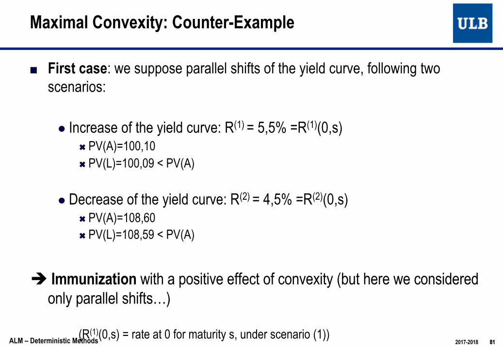
81
■ First case: we suppose parallel shifts of the yield curve, following twoscenarios:
● Increase of the yield curve: R(1) = 5,5% =R(1)(0,s)Ó PV(A)=100,10Ó PV(L)=100,09 < PV(A)
● Decrease of the yield curve: R(2) = 4,5% =R(2)(0,s)Ó PV(A)=108,60Ó PV(L)=108,59 < PV(A)
è Immunization with a positive effect of convexity (but here we considered only parallel shifts…)
(R(1)(0,s) = rate at 0 for maturity s, under scenario (1))
Maximal Convexity: Counter-Example
81ALM – Deterministic Methods 2017-2018
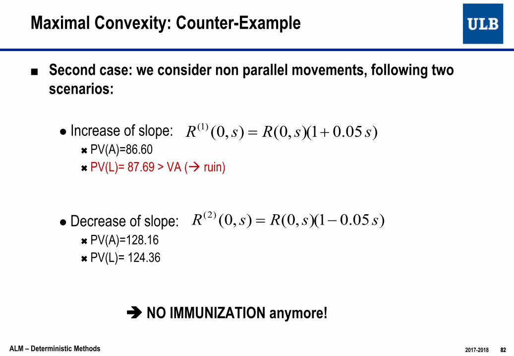
82
■ Second case: we consider non parallel movements, following twoscenarios:
● Increase of slope: Ó PV(A)=86.60Ó PV(L)= 87.69 > VA (à ruin)
● Decrease of slope:Ó PV(A)=128.16Ó PV(L)= 124.36
è NO IMMUNIZATION anymore!
Maximal Convexity: Counter-Example
2017-2018 82
)05.01(),0(),0()1( ssRsR +=
)05.01(),0(),0()2( ssRsR -=
ALM – Deterministic Methods

83
■ In summary:
Maximal Convexity: Counter-Example
V(A) 104.24 100.10 108.60 86.60 128.16 V(L) 104.24 100.09 108.59 87.69 124.36
t Flux A Flux P Initial Rates +0,5% -0,5% *(1+0,05*s) *(1-0,05*s)0 5.0% 5.5% 4.5% 5.0% 5.0%1 5.0% 5.5% 4.5% 5.3% 4.8%2 5.0% 5.5% 4.5% 5.5% 4.5%3 5.0% 5.5% 4.5% 5.8% 4.3%4 5.0% 5.5% 4.5% 6.0% 4.0%5 5.0% 5.5% 4.5% 6.3% 3.8%6 80 5.0% 5.5% 4.5% 6.5% 3.5%7 5.0% 5.5% 4.5% 6.8% 3.3%8 5.0% 5.5% 4.5% 7.0% 3.0%
8.564 158.31 5.0% 5.5% 4.5% 7.1% 2.9%10 5.0% 5.5% 4.5% 7.5% 2.5%11 5.0% 5.5% 4.5% 7.8% 2.3%12 80 5.0% 5.5% 4.5% 8.0% 2.0%
83ALM – Deterministic Methods 2017-2018

84
■ Cash-flow matching represents an extreme: all cash-flows are perfectly matched; it protects the liabilities portfolio against any possible movements of interest rates, BUT is in general difficult to implement in practice (often impossible)
■ Immunisation by duration is the other extreme, it only protects against smallparallel shifts
■ Vectorial duration allows to extend the immunisation concept to non parallel shifts of the yield curve.
Vectorial Duration
84ALM – Deterministic Methods 2017-2018

85
■ Different versions of vectorial duration can be considered
■ We consider here a modification of rates following 3 types of movements:
● Parallel● Linear (in maturity)● Quadratic (in maturity)
● This leads to one definition of vectorial duration● Considering other transformations lead to other definitions
Vectorial Duration
2017-2018 85
;..),0(),0( 2ssisRsR gh +++=Þ +
ALM – Deterministic Methods
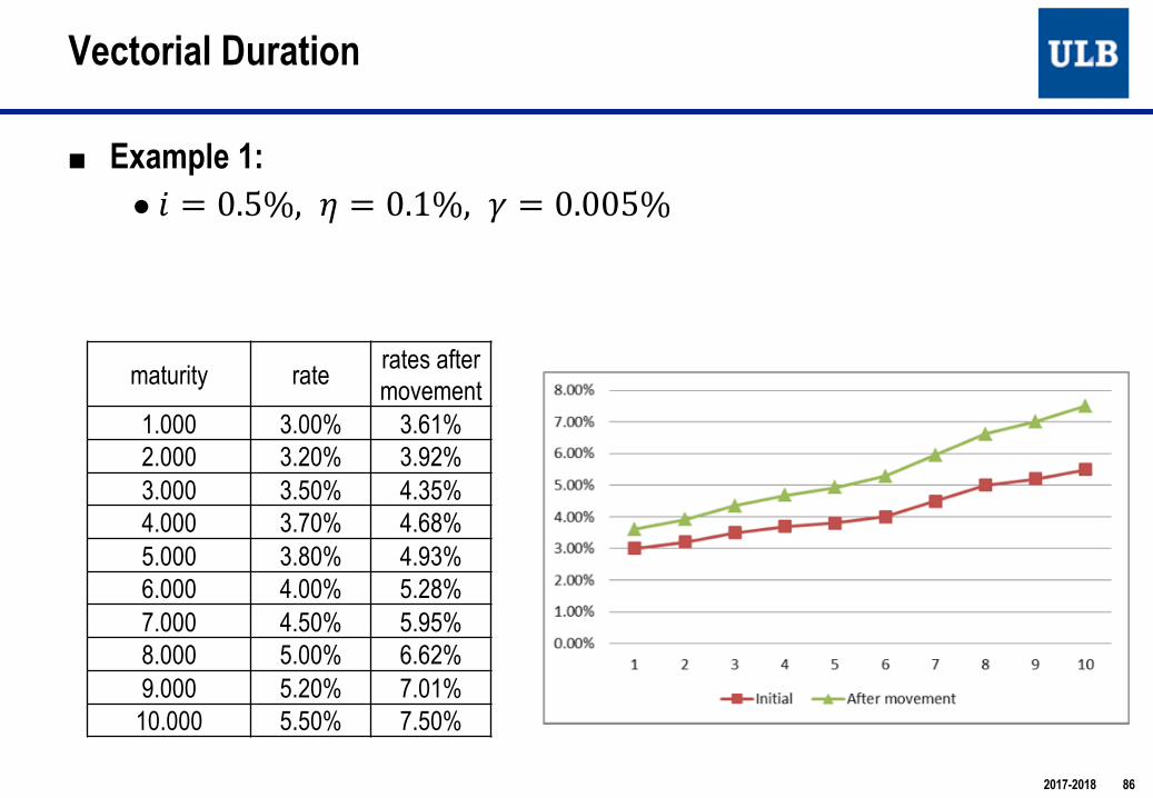
■ Example 1: ● ! = 0.5%, ( = 0.1%, * = 0.005%
Vectorial Duration
2017-2018 86
maturity rate rates after movement
1.000 3.00% 3.61%2.000 3.20% 3.92%3.000 3.50% 4.35%4.000 3.70% 4.68%5.000 3.80% 4.93%6.000 4.00% 5.28%7.000 4.50% 5.95%8.000 5.00% 6.62%9.000 5.20% 7.01%
10.000 5.50% 7.50%

■ Example 2:■ ! = −0.6%, ) = 0, * = 0.02%
Vectorial Duration
2017-2018 87
maturity rate rates after movement
1.000 3.00% 2.42%2.000 3.20% 2.68%3.000 3.50% 3.08%4.000 3.70% 3.42%5.000 3.80% 3.70%6.000 4.00% 4.12%7.000 4.50% 4.88%8.000 5.00% 5.68%9.000 5.20% 6.22%
10.000 5.50% 6.90%

88
■ If we only consider first order variations:
Vectorial Duration
2017-2018 88
))(0(
)0()0()0(
)0(),,,0(),,,0(
321 DDDiPV
PVPViPVi
PViPViPV
ghg
gh
h
ghgh
---=¶¶
+¶¶
+¶¶
@
-=D
ALM – Deterministic Methods
89
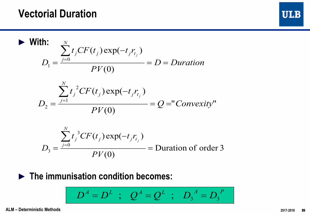
► With:
► The immunisation condition becomes:
Vectorial Duration
DurationDPV
rttCFtD
N
jtjjj j
==-
=å=
)0(
)exp()(0
1
"")0(
)exp()(1
2
2 ConvexityQPV
rttCFtD
N
jtjjj j
==-
=å=
89
3order ofDuration )0(
)exp()(0
3
3 =-
=å=
PV
rttCFtD
N
jtjjj j
PALALA DDQQDD 33;; ===ALM – Deterministic Methods 2017-2018

90
■ Let us come back to our previous example
■ We consider an initial yield curve with flat structure, equal to 5% (continuous rate).
■ Suppose we invest in two types of assets:● The first one generates a cash-flow of 80 currency units in 6 years;● The second one generates a cash-flow of 80 currency units in 12 years
■ Suppose that liabilities correspond to a unique cash-flow of 158,23 currency units in 8,55 years (like a ZC bond)
Vectorial Duration
90ALM – Deterministic Methods 2017-2018
91
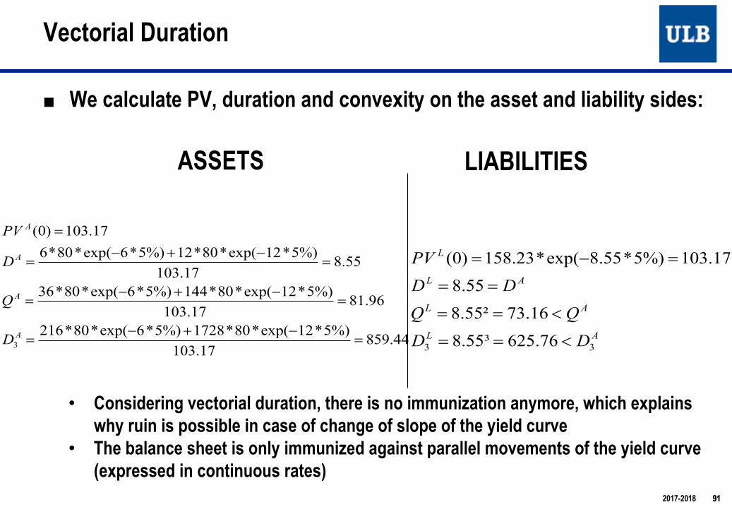
■ We calculate PV, duration and convexity on the asset and liability sides:
Vectorial Duration
44.85917.103
%)5*12exp(*80*1728%)5*6exp(*80*216
96.8117.103
%)5*12exp(*80*144%)5*6exp(*80*36
55.817.103
%)5*12exp(*80*12%)5*6exp(*80*617.103)0(
3 =-+-
=
=-+-
=
=-+-
=
=
A
A
A
A
D
Q
D
PV
AL
AL
AL
L
DDQQ
DDPV
33 76.625³55.816.73²55.8
55.8
17.103%)5*55.8exp(*23.158)0(
<==
<==
==
=-=
• Considering vectorial duration, there is no immunization anymore, which explainswhy ruin is possible in case of change of slope of the yield curve
• The balance sheet is only immunized against parallel movements of the yield curve(expressed in continuous rates)
LIABILITIESASSETS
912017-2018

■ Considering vectorial duration, immunization becomes:
■ Given a set of possible assets, this corresponds to solve in quantities!" the following system:
92
PV of assets = PV of liabilitiesDuration of assets = Duration of liabilitiesConvexity of assets = Convexity of liabilitiesDuration of order 3 of assets = Duration of order 3 of liabilities
Immunisation with vectorial duration
92ALM – Deterministic Methods 2017-2018
L
iasseti
i
assetasseti
DP
DP
i
i
i
2
2
=
å
å
a
aL
iasseti
i
assetasseti
DP
DP
i
i
i
1
1
=
å
å
a
aL
iasseti
i
assetasseti
DP
DP
i
i
i
3
3
=
å
å
a
a
Li
asseti PVPi=åa

■ In our example, if we suppose that we can invest in ZC bonds of maturities 5, 6, 10 and 12, of notional 100, this gives an (approx) solution:
■ And with the constraint that short selling is not allowed:
93
Immunisation with vectorial duration
93ALM – Deterministic Methods 2017-2018
alpha1 -0.47977alpha2 1.025055alpha3 1.33156alpha4 -0.29457
alpha1 0alpha2 0.62679alpha3 0.935429alpha4 0
Assets liabilitiesPV 103.1704 103.1704D1 8.199725 8.553345D2 71.1956 73.15971D3 647.1461 625.7602
Assets liabilitiesPV 103.1704 103.1704D1 8.553238 8.553345D2 73.16064 73.15971D3 625.7577 625.7602

94
■ If we consider non parallel movements, following two scenarios(we consider the first case solution):
● Increase of slope: Ó PV(A)=71.57Ó PV(L)= 71.56
● Decrease of slope:Ó PV(A)=110.998Ó PV(L)= 111.001
Ó In fact we still have possible ruin but with a shortfall much smaller than before (almost negligible here)
Ó See example in Excel
Vectorial Duration
2017-2018 94
ssRsR 005.0),0(),0()1( +=
ALM – Deterministic Methods
ssRsR 001.0),0(),0()2( -=
95
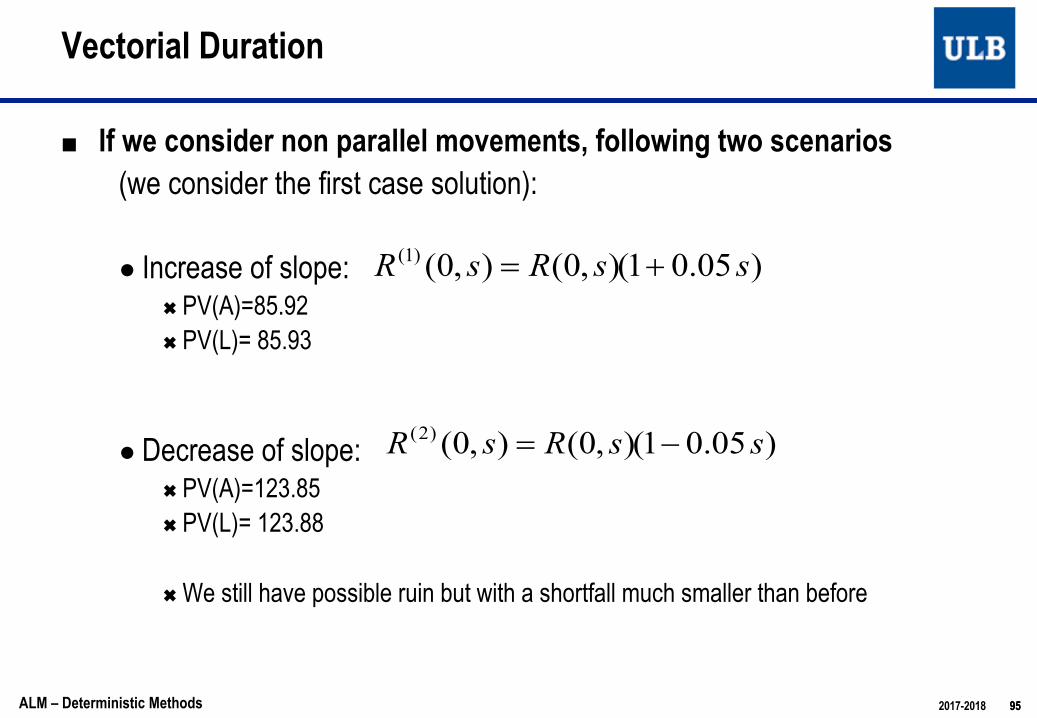
■ If we consider non parallel movements, following two scenarios(we consider the first case solution):
● Increase of slope: Ó PV(A)=85.92Ó PV(L)= 85.93
● Decrease of slope:Ó PV(A)=123.85Ó PV(L)= 123.88
Ó We still have possible ruin but with a shortfall much smaller than before
Vectorial Duration
2017-2018 95
)05.01(),0(),0()1( ssRsR +=
)05.01(),0(),0()2( ssRsR -=
ALM – Deterministic Methods

96
■ If we suppose that all movements of the yield curve are parallel, then the classical immunisation condition, with a maximisation of the convexityof assets, appears sufficient
■ Now, if we want to protect an insurance portfolio against non parallelmovements, immunization using only (first order) duration appears not sufficient, and durations of superior orders must be considered
● In particular the maximum convexity is not always a good idea…
■ The company can define the types of yield curve deformations againstwhich it desires to hedge, and consider the corresponding (vectorial) duration notions in order to perform the adequate protection
Immunization and ALM
96ALM – Deterministic Methods 2017-2018

97
■ Let us consider a portfolio composed of two instruments:● A fixed rate bond, with maturity TN , coupon rbond and notional = 1● A forward receiver swap beginning at TN, of maturity !" > !$ and
notional 1
■ One can show that the value of this forward receiver swap at t is givenby:
where rswap is the fixed rate of the swap (possibly different from the forward swap rate, because e.g. the swap was concluded some time before t)
Swaps and Duration (1/3)
( )å+=
- +--M
NiMZCNZCiZCiiswap TtPTtPTtPTTr
11 ),(),(),(
97ALM – Deterministic Methods 2017-2018

98
■ Then the value of the portfolio (forward swap + bond) at t is equal to:
à This new portfolio has a duration much closer to !" in practice (it has the duration of a bond of maturity #")
à Adding a forward swap to a fixed rate bond, of maturity equal to the maturity of the bond, allows to increase the duration of assets§ This can be useful when bonds of sufficiently high maturity cannot be found on
the market
Swaps and Duration (2/3)
( )
( )
( ) ( )
MswapNbond
M
M
NiMZCiZCiiswap
N
iiZCiibond
M
NiMZCNZCiZCiiswap
N
iNZCiZCiibond
TrTrT
TtPTtPTTrTtPTTr
TtPTtPTtPTTr
TtPTtPTTr
until and , until level a :levelscoupon different 2but with ,maturity of bond a of Price
),(),(),(
),(),(),(
),(),((t)V
11
11
11
11Portfolio
=
+-+-=
+--+
+-=
åå
å
å
+=-
=-
+=-
=-
98ALM – Deterministic Methods 2017-2018

99
■ Now, considering the duration of the swap on a standalone basis makesfew sense at the moment of its conclusion and it the fixed rate of the swap, !"#$%, is equal to the forward swap rate of the market.
■ In this case the value at conclusion of the forward swap is 0, and itsduration (at conclusion) is not defined
● It is infinite, and can take (just) after conclusion all possible values between +∞ and −∞ , depending on movements of the yield curve afterthat conclusion
■ But if the fixed rate of the swap is « sufficiently higher » than the forwardswap rate at instant t, then its duration will become positive. It also tends to +, − +- if rates become « much higher » than the fixed rate
Swaps and Duration (3/3)
2017-2018 99ALM – Deterministic Methods

100
■ The static approach may introduce some distorsion in the perception of risks by the company:
■ It focusses on interest rate risk, and only on small movements of the yield curve. In particular, we ignore:
● Other market risks than interest rate risk● Risks linked to the behaviour of policyholders
■ Immunisation based on duration is efficient only if cash-flows are close to deterministic, independent of interest rates, which is not the case
■ The static approach methodologies ignore interactions between assetsand liabilities
● It does not take into account future production (new contracts) or profit sharing
■ Conclusion: The static approach is limited and sometimes not welladapted to the nature of liabilities of an insurance company
Limitations of the Static Approach
100ALM – Deterministic Methods 2017-2018

101
■ New elements are taken into account in the dynamic approach, mainly:● Interactions between assets and liabilities;● The entire term structure of interest rates can move under non parallel and
unlimited movements;● Other financial risks than interest rates risk are taken into account.
■ This approach is however not yet stochastic
■ It is based on projections of cash-flows under deterministic scenarios● Sensitivity analysis with respect to different variables, not only interest
rates● Stress scenarios
Second Generation Tools
101ALM – Deterministic Methods 2017-2018
102
■ Stress scenarios are based on deterministic scenarios « arbitrarily » defined by the analyst
● Stress on 1 variable● Stress on several variables at once
■ In general stress tests and scenarios can be established from:● Past observation of important events (past crises)● Observed percentiles of market and economic variables, from historical
time series● Percentiles obtained from stochastic models, calibrated on past data
■ The definition of scenarios should ideally reflect consistency betweenthe different variables
■ Once the scenarios have been defined, we analyse their impact on the balance sheet (and cash-flows)
Stress Testing – Scenarios Analysis (1/2)
102ALM – Deterministic Methods 2017-2018

103
■ Stress testing and scenario analysis provides information about the limiting conditions under which the company is still alive
● Close to reverse stress testing
■ We consider a broader set of scenarios, we are not anymore limited to small parallel movements of interest rates
■ For instance: ● Possiblity to test for each scenario different asset allocation strategies, and to consider in
extreme scenarios the trade-off between profit, concurrence and solvency.
■ The examination of extreme scenarios provides a first assessment of itssolvency
■ It also allows the company to manage crisis situations before theyhappen
Stress Testing – Scenarios Analysis(2/2)
103ALM – Deterministic Methods 2017-2018

104
■ Example of Interest rates scenarios● Rates unchanged● Progressive increase of 5% in 5 years, followed by a progressive decrease of 5% in 5
years, then rates unchanged● Instantaneous increase of 3%, then rates unchanged● Progressive decrease of 5% in 10 years then rates unchanged● Progressive decrease of 5% in 5 years, followed by a progressive increase of 5% in 5
years, then rates unchanged● Instantaneous decrease of 3%, then rates unchanged
■ These scenarios are generally also associated to movements in the equitymarket.
● e.g. instantaneous equity crash of -30%, or stagnation, or immediate increase of 10%...
■ Coherence between different variables ● Can be achieved based on regression analyses (e.g. of stock indices or real estate indices
on interest rates,…)
Examples
104ALM – Deterministic Methods 2017-2018

105
■ The values of assets and liabilities will be projected along severalscenarios
■ At the beginning of period n (i.e. at tn-1), the level of stocks of assets and liabilities are known
■ In practice, it is convenient to distinguish three moments at the end of each period (i.e. at tn):
● Before rebalancing and before reinvestment : the value of assets is computed on the basis of economic scenarios: new values of stocks, bonds, real estate… (effect of the market)
● After rebalancing but before reinvestment: we rebalance (reallocation) the assetsportfolio following the asset allocation strategy
● After rebalancing and after reinvestment : the total net cash-flow for the period iscalculated, and is de- or re-invested in assets, following the asset allocation strategy. If itis negative, we desinvest, otherwise we invest.
Balance Sheet Analyses
105ALM – Deterministic Methods 2017-2018

106
■ Interactions will be taken into account■ They are multiple:
● Behaviour of the policyholders: modelled by a function introduced by the modeller. The behaviour of policyholders will be used by the model alongscenarios.
Ó For instance surrender rates will be function of interest rates, or function of the age of the contract itself and the characteristics of the insured…
● The net cash-flow is calculated at the end of each period, and reinvestment must be performed.
● Profit sharing: will in general be linked with the economic conditions of the considered scenario
Ó E.g. profit sharing of 2% in a scenario in which assets have overperformed, or if rates in the market have increased a lot, nothing in a scenario in which assets have decreased a lot, or if rates stay at very low levels in the market
Interactions between assets and liabilities
106ALM – Deterministic Methods 2017-2018
107
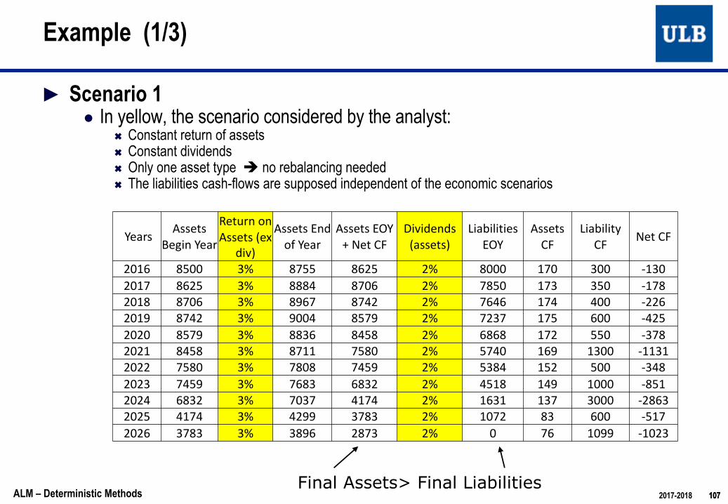
► Scenario 1● In yellow, the scenario considered by the analyst:
Ó Constant return of assetsÓ Constant dividendsÓ Only one asset type è no rebalancing neededÓ The liabilities cash-flows are supposed independent of the economic scenarios
Example (1/3)
Final Assets> Final Liabilities107
Years AssetsBegin Year
Return on Assets (ex
div)
Assets End of Year
Assets EOY + Net CF
Dividends (assets)
LiabilitiesEOY
AssetsCF
LiabilityCF Net CF
2016 8500 3% 8755 8625 2% 8000 170 300 -1302017 8625 3% 8884 8706 2% 7850 173 350 -1782018 8706 3% 8967 8742 2% 7646 174 400 -2262019 8742 3% 9004 8579 2% 7237 175 600 -4252020 8579 3% 8836 8458 2% 6868 172 550 -3782021 8458 3% 8711 7580 2% 5740 169 1300 -11312022 7580 3% 7808 7459 2% 5384 152 500 -3482023 7459 3% 7683 6832 2% 4518 149 1000 -8512024 6832 3% 7037 4174 2% 1631 137 3000 -28632025 4174 3% 4299 3783 2% 1072 83 600 -5172026 3783 3% 3896 2873 2% 0 76 1099 -1023
ALM – Deterministic Methods 2017-2018

Assets Begin Year
Return on Assets (ex
div)
Assets End of Year
Assets EOY + Net CF
Dividends (assets)
Liabilities EOY
Assets CF
Liability CF Net CF
2016 8500 0% 8500 8370 2% 8000 170 300 -1302017 8370 -5% 7952 7769 2% 7850 167 350 -1832018 7769 -5% 7380 7136 2% 7646 155 400 -2452019 7136 -5% 6779 6322 2% 7237 143 600 -4572020 6322 -5% 6006 5582 2% 6868 126 550 -4242021 5582 0% 5582 4394 2% 5740 112 1300 -11882022 4394 3% 4526 4113 2% 5384 88 500 -4122023 4113 3% 4237 3319 2% 4518 82 1000 -9182024 3319 3% 3419 485 2% 1631 66 3000 -29342025 485 3% 500 -91 2% 1072 10 600 -5902026 -91 3% -93 -1194 2% 0 -2 1099 -1100
► Scenario 2:● Decreasing returns● Constant dividends● The liabilities cash-flows are supposed independent of the economic scenarios
108
Example(2/3)
End 2017: Assets < Liabilities
Assets in 2025 < 0108ALM – Deterministic Methods 2017-2018

Assets Begin Year
Return on Assets (ex
div)
Assets End of Year
Assets EOY + Net CF
Dividends(assets)
LiabilitiesEOY
Assets CF
Liability CF Net CF
2016 8500 2.5% 8713 8583 2% 8000 170 300 -1302017 8583 2.5% 8797 8619 2% 7850 172 350 -1782018 8619 0.0% 8619 8391 2% 7646 172 400 -2282019 8391 0.0% 8391 7959 2% 7237 168 600 -4322020 7959 0.0% 7959 7568 2% 6868 159 550 -3912021 7568 -2.5% 7379 6230 2% 5740 151 1300 -11492022 6230 -2.5% 6074 5699 2% 5384 125 500 -3752023 5699 -2.5% 5557 4671 2% 4518 114 1000 -8862024 4671 -2.5% 4554 1647 2% 1631 93 3000 -29072025 1647 -2.5% 1606 1039 2% 1072 33 600 -5672026 1039 -2.5% 1013 -65 2% 0 21 1099 -1078
109
► Scenario 3:● Decreasing returns● Decreasing dividends● The liabilities cash-flows are supposed independent of the economic scenarios
Example(3/3)
Assets < Liabilities109ALM – Deterministic Methods 2017-2018

110
■ Scenarios are defined arbitrarily, but the aim is here to:● Be able to anticipate reactions to adopt in case of specific crisis situations;● Detect weaknesses of strategies (asset allocation, profit sharing policies…)
■ Model risk:● Complexity of models in practice à risk that the model is badly used, risk of bad
interpretations ● Risk that the different assumptions are not coherent (difficulty to build coherent
scenarios)
■ Communication:● A good communication of assumptions, results and context of the model is
important. ● Communication to management ● Better use a restricted number of scenarios , in order to keep a clear view of the
situation
Second generation tools: limitations (1/2)
2017-2018 110ALM – Deterministic Methods

111
■ Scenarios are not weighted by probabilities, and cannot be aggregatedin order to produce risk measures (like economic or regulatory capital)
■ Third generation tools : stochastic models
■ Rem: it is possible to define an approach by deterministic scenarios (hence a limited number of balance sheet and cash-flow projections) where scenarios themselves are based on stochastic models
● Scenarios correspond to percentiles of some market variables ● Possibility to obtain in this approach some quantification of risks, and
derive some capital level● Possible mixture between stochastic methods and deterministic
projections● Actually, this appears as a proxy of a pure stochastic model
Second generation tools: limitations(2/2)
2017-2018 111ALM – Deterministic Methods