Finance and Growth - Mathematics for Economics: enhancing

Teaching and Learning

Guide 5:

Finance and Growth

Teaching and Learning Guide 5: Finance and Growth

of 37

Table of Contents

Section 1: Introduction to the guide ............... ................................................... 3 Section 2: Arithmetic & Geometric Sequences and Ser ies.............................. 4

1. The concept of Arithmetic & Geometric Sequences and Series............................................4 2. Presenting the concept of Arithmetic & Geometric Sequences and Series...........................4 3. Delivering the concept of Arithmetic & Geometric Sequences and Series to small and larger groups .......................................................................................................................................6 4. Discussion.............................................................................................................................7 5. Activities................................................................................................................................7 6. Top tips ……..…………………………………………………………………………………….. 12 7. Conclusion ..........................................................................................................................13

Section 3: Simple and Compound Interest............ .......................................... 14 1. The concept of simple and compound Interest ...................................................................14 2. Presenting the concept of simple and compound Interest...................................................15 4. Discussion...........................................................................................................................17 5. Activities..............................................................................................................................17

6. Top tips …..……………………………………………………………………………………….. 24 Section 4: Investment Appraisal .................... .................................................. 24

1. The concept of investment appraisal...................................................................................24 2. Presenting the concept of investment appraisal..................................................................24 3. Delivering the concept of investment appraisal to small and larger groups.........................25 4. Discussion...........................................................................................................................29 5. Activities..............................................................................................................................29 6. Top tips ……………………………………………………………………………………………. 37 7. Conclusion ..........................................................................................................................37


of 37

Section 1: Introduction to the guide

This Guide is designed to set out some of the basic mathematical concepts needed to teach

financial economics at undergraduate level. The concepts covered by this guide are:

- Arithmetic and geometric series;

- Simple and compound interest;

- The time value of money;

- Investment appraisal; and

- The NPV rule and the IRR rate of return rule.

The modern day finance lecturer is fortunate in the number of real world examples they have

available to them. This Guide provides a number of current examples covering borrowing,

investment and annuities to support the delivery of core concepts. The lecturer is encouraged to

revisit the sources cited to update the examples nearer the time of delivery.

The use of Excel is an essential tool for anyone working in finance. Throughout this guide Excel

screenshots and links to files are provided. It would be useful therefore if the session utilising

this material were presented in a classroom where students can gain hands on experience.

A large part of this guide is devoted to “Teaching and Learning” exercises. Years of teaching

this discipline have led this author to believe that this is definitely a “doing” subject and with lots

of hands on practise the concepts should be easier to understand. This guide utilises a number

of mathematic concepts explored in other guides in the series, namely: (i) the use of the

summation notation; (ii) use of natural logarithms; (iii) use of the exponential function; (iv) the

quadratic equation; (v) finding the equation of a straight line.


of 37

Section 2: Arithmetic & Geometric Sequences and Ser ies

1. The concept of Arithmetic & Geometric Sequences and Series Many students will have little idea exactly what is meant by a ‘mathematical series’ and it is

likely that fewer still will have a grasp that mathematics can be used to help solve problems

regarding finance and growth. Lecturers might find it advantageous to start this material with a

simple and clear explanation of the terms, “finance”, “income”, “wealth” and “growth”. For

example,

‘Finance’ refers to a wide range of economic activities which are concerned with the

management of income and wealth.

‘Income’ can be defined as income is defined as a stream of payments which are received in

return for providing something: Apple Corporation for example received huge incomes from

selling more than 14 million of its iPod personal music players in the last three months of 2005.

‘Wealth’ on the other hand is a ‘stock concept’ and refers to the accumulation of valuables or

assets over time e.g. the Russian businessman Roman Abramovich has an estimated wealth of

around £10 billion1.

‘Growth’ means the increase (if it’s positive) or decrease (if it is negative) in the size of

something over a given period of time e.g. during the Summer of 2007 it was reported that

Crops in the Black Sea area of Europe, were ruined by bad weather with Chinese production of

wheat expected to fall by 10% as a result of both flooding and droughts. These examples will

help students to appreciate that series are about systematic changes in economic variables

over time. Students could be encouraged to research their own stories regarding growth.

2. Presenting the concept of Arithmetic & Geometric Sequences and Series Students will need to be clear about the difference between an arithmetic progression and a

geometric progression. The labels themselves are opaque and probably quite off-putting so a

restatement is crucial.


of 37

The following could be useful introductory presentation:

Arithmetic Progression

An arithmetic series (or progression) is a series in which there is a constant difference

between each term. For example:

100, 101, 102, 103, 104….

3, 7, 11, 15, 19….

The distinct feature of these series (or sequences) is that each term, after the first, is obtained

by adding a constant, d, to the previous term. In the examples above, ‘d’ is 1 and 4 respectively.

In the discussion that follows ‘a’ is used to represent the first term.

Each element of a series (or sequence) can be identified by reference to its position in the

sequence (or its term number). For example, in the second series above, the first term, T1, of

the sequence is a = 3 and the second term, T2, of the sequence is a + d = 3 + 4 = 7. Hence the

value of any term can be determined with reference to the values for ‘a’ and ‘d’ and its position

in the sequence.

This is best illustrated in tabular form:

Value 3 7 11 15 .. ..

Sequence a a + d a + 2d a + 3d a + (n-1)d

Term number T1 T2 T3 T4 Tn

Equally, the overview of a geometric progression would also need to be provided:

Geometric Progression

A geometric series (or progression) is one in which there is a constant ratio between any two

geometric terms. For example:

1, 10, 100, 1000, 10000,….

1 Source: The Times Rich List 2006


of 37

3, 9, 27, 81, 243,….

The distinct feature of these series is that each term, after the first, is obtained by multiplying the

previous term by a constant, r. In the examples above, ‘r’ is 10 and 3 respectively. Again, in the

discussion that follows ‘a’ is used to represent the first term.

Each element of a sequence can be identified by reference to its position in the sequence (or its

term number). For example, in the second series above, the first term, T1, of the sequence is a

= 3 and the second term, T2, of the sequence is ar = 3 x 3. The third term, T3, is ar2 = 3 x 32.

Hence the value of any term can be determined with reference to the values for ‘a’ and ‘r’ and

its position in the sequence.

In tabular form:

Value 3 9 27 81 .. ..

Sequence a ar ar2 ar3 ar(n-1)

Term number T1 T2 T3 T4 Tn

3. Delivering the concept of Arithmetic & Geometric Sequences and Series to small and larger groups Students could benefit from watching one or more clips regarding geometric series (See Video

clips immediately below) and then watch a clip on their own or in pairs and then report back to

the group:

- What the clip was about;

- What the economic issue was ie. What was the presenter trying to explain?

- How geometric series could be used to solve the problem or issue.

Links to the online question bank

This Guide draws upon complementary knowledge eg. logarithms, fractions etc and so students

might wish to practise these underpinning concepts at

http://www.metalproject.co.uk/METAL/Resources/Question_bank/Algebra/index.html

and http://www.metalproject.co.uk/METAL/Resources/Question_bank/Numbers/index.html


of 37

Video clips

A useful general clip on the practical application of series, growth and investments can be found

at: http://www.metalproject.co.uk/Resources/Films/Mathematics_of_finance/index.html under

3.08 “Eurotunnel - A Bad Investment”. This could to ‘set the scene’ for this topic.

There are several useful clips dedicated to geometric series. These can also be found at

http://www.metalproject.co.uk/Resources/Films/Mathematics_of_finance/index.html.

4. Discussion Students could be asked to consider ways in which other variables or phenomena can grow or

change over time. For example, how bacteria grow or how a forest fire can appear to devour

parkland with an increasing speed. This could be linked to economic issues such as how stock

markets can respond with ‘increasing pessimism’ as result of expectations – eg. the Wall Street

Crash – and the notion of the rate of change becoming more rapid.

5. Activities Learning Objectives

LO1: Students to understand the meaning of ‘geomet ric series’

LO2: Students to learn how to calculate a geometric series and the constant ratio

LO3: Students to learn the meaning of ‘compound int erest’

LO4: Students to learn how to independently calcula te compound interest.

ACTIVITY ONE

Background and Worked Example

One of the applications of geometric series is the calculation of compound interest. Here the

sum on which interest is paid includes the interest that has been earned in previous years.

For example, if £100 is invested at 5% per annum compound interest, then after 1 year the

interest earned is £5 (100 x 0.05) and the capital invested for the second year is £105. The

interest earned in the second year is then £5.25 (£105 x 0.05) and this capital amount is carried

forward to year 3.


of 37

Presenting this in tabular form:

Beginning of

year

1 2 3 4 5

Capital 100 105 110.25 115.7625 121.550625

Interest during

the year

100 x

0.05 = 5

105 x 0.05

= 5.25

110.25 x 0.05

= 5.5125

115.7625 x 0.05 =

5.788125

Reproducing the table in algebraic form with ‘a’ representing capital and ‘i’ representing the rate

of interest (in decimal form):

Beginning of

year 1 2 3 4 5

Capital a a + ai =

a(1+i)

a(1+i) +

a(1+i)i= a(1+i)2

a(1+i)2+ a(1+i)2i =

a(1+i)2(1+i) = a(1+i)3

a(1+i)3+ a(1+i)3i

= a(1+i)3(1+i)=

a(1+i)4

Interest during

the year ai a(1+i)i a(1+i)2i

a(1+i)3i

Therefore the value in year n is a(1+i)n-1. Hence the example above with a = 100, i = 0.05, the

value at the beginning of year 5 is:

100 x (1 + 0.05)4 = 121.550625

The sum of a geometric series is obtained easily by considering the series in its algebraic form

(see table above):

a, ar, ar2, ar3, …., arn-1

The sum of the first n terms is:


of 37

Sn = a + ar + ar2 + ar3 +…+ arn-1

Multiplying both sides by r:

rSn = ar + ar2 + ar3 + ar4 + …+ arn

(since arn-1 x r = arn-1+1 = arn)

Subtracting rSn from Sn gives:

Sn – rSn = a – arn

Hence:

Sn = (a – arn)/(1 – r) = a(1 – rn)/(1 – r)

Example 1:

Find the sum of the first 10 terms of the series

8, 4, 2, 1,…..

This is a geometric series since each term is obtained by multiplying the previous term by 0.5.

Applying the formula above, the sum of the first 10 terms is:

S10 = 8(1 – 0.510)/(1 – 0.5) = 16 x (1 – 0.00098) = 15.98

Note the calculation of rn yields a very small value of 0.00098 and as ‘n’ gets larger this value

can only get smaller, e.g.

0.55 = 0.03125, 0.515 = 0.000031

Hence if the series has an infinite number of terms, rn will be so small that in practise it will be

zero. The formula for the sum of an infinite geometric progression is then:

Sn = a(1 – 0)/(1 – r) = a/(1- r)


of 37

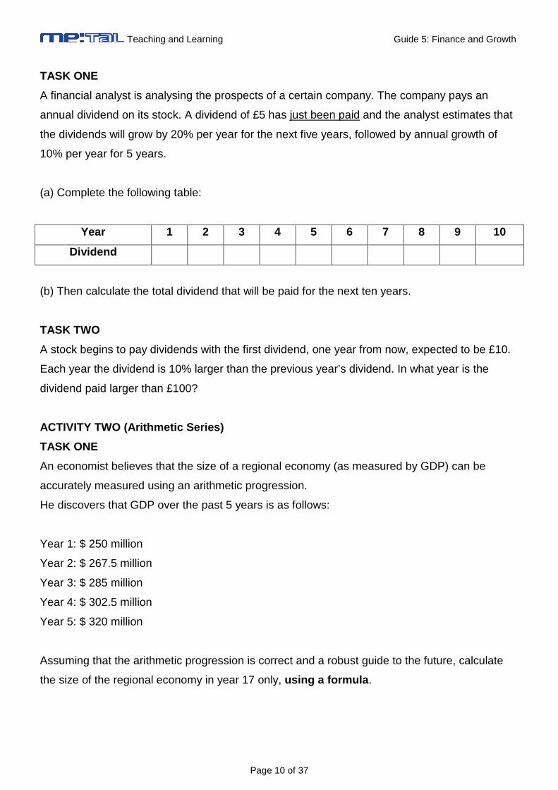
TASK ONE

A financial analyst is analysing the prospects of a certain company. The company pays an

annual dividend on its stock. A dividend of £5 has just been paid and the analyst estimates that

the dividends will grow by 20% per year for the next five years, followed by annual growth of

10% per year for 5 years.

(a) Complete the following table:

Year 1 2 3 4 5 6 7 8 9 10

Dividend

(b) Then calculate the total dividend that will be paid for the next ten years.

TASK TWO

A stock begins to pay dividends with the first dividend, one year from now, expected to be £10.

Each year the dividend is 10% larger than the previous year’s dividend. In what year is the

dividend paid larger than £100?

ACTIVITY TWO (Arithmetic Series)

TASK ONE

An economist believes that the size of a regional economy (as measured by GDP) can be

accurately measured using an arithmetic progression.

He discovers that GDP over the past 5 years is as follows:

Year 1: $ 250 million

Year 2: $ 267.5 million


Year 4: $ 302.5 million


Assuming that the arithmetic progression is correct and a robust guide to the future, calculate

the size of the regional economy in year 17 only, using a formula .


of 37

ANSWERS

ACTIVITY ONE

TASK ONE

(a)

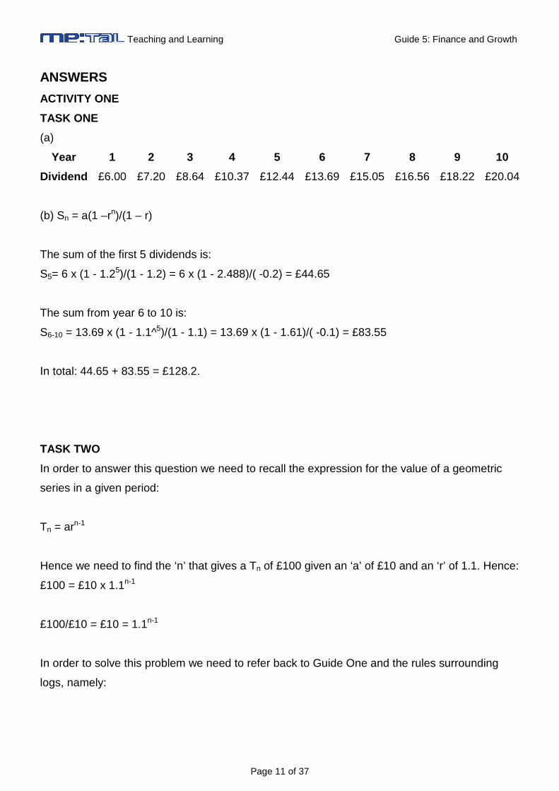
Year 1 2 3 4 5 6 7 8 9 10

Dividend £6.00 £7.20 £8.64 £10.37 £12.44 £13.69 £15.05 £16.56 £18.22 £20.04

(b) Sn = a(1 –rn)/(1 – r)

The sum of the first 5 dividends is:

S5= 6 x (1 - 1.25)/(1 - 1.2) = 6 x (1 - 2.488)/( -0.2) = £44.65

The sum from year 6 to 10 is:

S6-10 = 13.69 x (1 - 1.1^5)/(1 - 1.1) = 13.69 x (1 - 1.61)/( -0.1) = £83.55

In total: 44.65 + 83.55 = £128.2.

TASK TWO

In order to answer this question we need to recall the expression for the value of a geometric

series in a given period:

Tn = arn-1

Hence we need to find the ‘n’ that gives a Tn of £100 given an ‘a’ of £10 and an ‘r’ of 1.1. Hence:

£100 = £10 x 1.1n-1

£100/£10 = £10 = 1.1n-1

In order to solve this problem we need to refer back to Guide One and the rules surrounding

logs, namely:


of 37

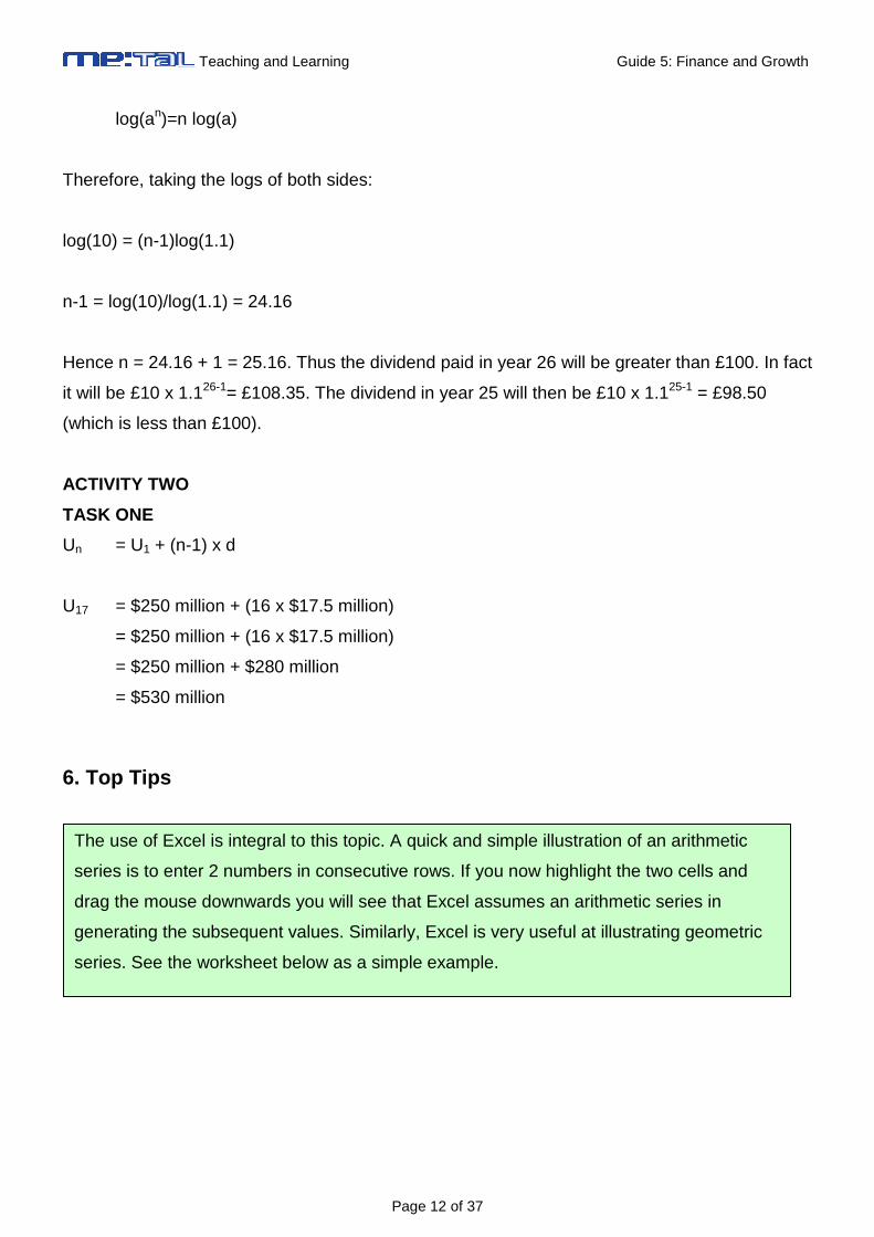
log(an)=n log(a)

Therefore, taking the logs of both sides:

log(10) = (n-1)log(1.1)

n-1 = log(10)/log(1.1) = 24.16

Hence n = 24.16 + 1 = 25.16. Thus the dividend paid in year 26 will be greater than £100. In fact

it will be £10 x 1.126-1= £108.35. The dividend in year 25 will then be £10 x 1.125-1 = £98.50

(which is less than £100).

ACTIVITY TWO

TASK ONE

Un = U1 + (n-1) x d

U17 = $250 million + (16 x $17.5 million)

= $250 million + (16 x $17.5 million)

= $250 million + $280 million

= $530 million

6. Top Tips

The use of Excel is integral to this topic. A quick and simple illustration of an arithmetic

series is to enter 2 numbers in consecutive rows. If you now highlight the two cells and

drag the mouse downwards you will see that Excel assumes an arithmetic series in

generating the subsequent values. Similarly, Excel is very useful at illustrating geometric

series. See the worksheet below as a simple example.


of 37

By varying the values for ‘a’ and ‘r’ you can generate a new geometric series.

7. Conclusion

Students should be encouraged to work thorough problem sets to help them develop their

mathematical skills and confidence. This underpinning and knowledge and competency will be

needed for subsequent material.


of 37

Section 3: Simple and Compound Interest

1. The concept of simple and compound Interest As noted earlier, students will benefit from clear and cogent definitions at the beginning of the

topic or module.

Definition of Simple Interest

Simple interest is a fixed percentage of the principal, P, that is paid to an investor each year,

irrespective of the number of years the principal has been left on deposit. Consequently an

amount of money invested at simple interest will increase in value by the same amount each

year.

Algebraically, the amount of simple interest, I, earned on a deposit, P0, invested at r% for t years

is:

I = P0 x r x t

Hence the total amount of money after t years is the principal plus the accrued interest:

P0 + P0 x r x t = P0(1 + rt)

Definition of compound interest

The view above of only the principal earning interest is a very simplistic one and normally the

interest on money borrowed is usually “compounded”. Compound interest pays interest on the

principal plus on any interest accumulated in previous years.

The total value after t years when a principal, P0, is compounded at r% per annum is:

Pt = P0(1+r)t


of 37

2. Presenting the concept of simple and compound Interest Worked examples are a good way for students to understand and apply the concepts and

mathematical techniques. They also provide a reference for students to return if they need to

when they are working independently on problem sets. Two worked examples are provided

below to help colleagues present these two concepts.

Presenting the calculation of simple interest

If you borrow £1000 for five years at a simple interest rate of 10% p.a., the amount of interest

you pay is:

I = P0 x r x t = £1000 x 0.1 x 5 = £500

Thus the cost of borrowing £1000 for five years at 10% p.a. simple interest is £500. The total

amount due after five years would be:

P0(1 + rt) = £1000 x (1 + 0.1 x 5) = £1500.

Presenting the calculation of compound interest

In order to demonstrate the fundamentals of compound interest consider a deposit of £1000

over 5 years at 10% per annum with interest compounded annually.

Principal at start

of year

Interest paid

each year

Total at end of

year

£1000 £100 £1100

£1100 £110 £1210

£1210 £121 £1331

£1331 £133.10 £1464.10

£1464.10 £146.41 £1610.51

Note the £1610.51 could have been obtained directly as:

£1000 x (1 + 0.1)5 = £1000 x 1.61051 = £1610.51


of 37

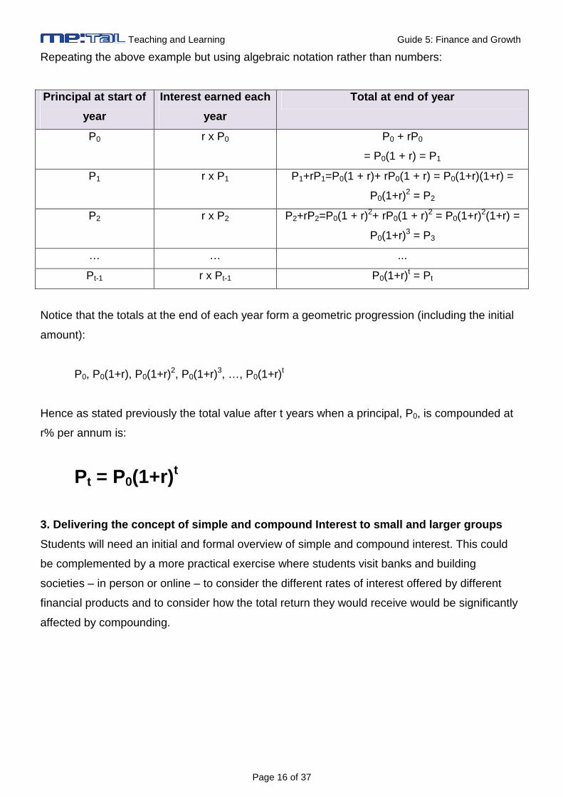
Repeating the above example but using algebraic notation rather than numbers:

Principal at start of

year

Interest earned each

year

Total at end of year

P0 r x P0 P0 + rP0

= P0(1 + r) = P1

P1 r x P1 P1+rP1=P0(1 + r)+ rP0(1 + r) = P0(1+r)(1+r) =

P0(1+r)2 = P2

P2 r x P2 P2+rP2=P0(1 + r)2+ rP0(1 + r)2 = P0(1+r)2(1+r) =

P0(1+r)3 = P3

… … ...

Pt-1 r x Pt-1 P0(1+r)t = Pt

Notice that the totals at the end of each year form a geometric progression (including the initial

amount):

P0, P0(1+r), P0(1+r)2, P0(1+r)3, …, P0(1+r)t

Hence as stated previously the total value after t years when a principal, P0, is compounded at

r% per annum is:

Pt = P0(1+r) t

3. Delivering the concept of simple and compound Interest to small and larger groups

Students will need an initial and formal overview of simple and compound interest. This could

be complemented by a more practical exercise where students visit banks and building

societies – in person or online – to consider the different rates of interest offered by different

financial products and to consider how the total return they would receive would be significantly

affected by compounding.


of 37


There are questions on investment appraisal including simple and compound interest at

http://www.metalproject.co.uk/METAL/Resources/Question_bank/Economics%20applications/in

dex.html

Video clips

The video clips for this Guide can be found at

http://www.metalproject.co.uk/Resources/Films/Mathematics_of_finance/index.html

Clips 3.01 to 3.03 (inclusive) offer good practical illustrations of compounding starting with an

applied example of a student calculating how long it will take for them to save for a round the

world trip.

4. Discussion A simple competition and discussion could be created where students are paired and given a

notional £1000 and a 10 year investment time frame and asked to select a savings account

which would maximise their compounded interest. Higher ability students could look at foreign

savings products and could factor in exchange rates when arriving at the Sterling figure.

5. Activities Learning Objectives

LO1: Students learn the meaning of key financial te rms- bond, coupon, interest, simple

and compound interest

LO2: Students learn how to calculate simple and com pound interest

LO3: Students learn the distinction between simple and compound interest

LO4: Students learn the impact which the frequency of compounding has upon the size

of the total return

Task One

A bond's coupon is the annual interest rate paid on the issuer's borrowed money, generally paid

out semi-annually. The coupon is always tied to a bond's face or par value , and is quoted as a

percentage of par. For instance, a bond with a par value of £1,000 and an annual interest rate

of 4.5% has a coupon rate of 4.5% (£45).


of 37

Say you invest in a six-year bond paying 5% per year, annually. Assuming you hold the bond to

maturity, you will receive 6 interest payments of £250 each, or a total of £1,500. Plus the par

value of £1000.This coupon payment is simple interest.

You can do two things with that simple interest—spend it or reinvest it. Determine the total

amount of money you will have after six years, assuming you can reinvest the interest at 5% per

annum.

Task Two

So far, it has been assumed that compound interest is compounded once a year. In reality

interest may be compounded several times a year, e.g. daily, weekly, monthly, quarterly, semi-

annually or even continuously.

The value of an investment at the end of m compounding periods is:

Pt = P0[1 + r/m]m x t

Where m is the number of compounding periods per year and t is the number of years.

Using this information, solve the following problem:

(a) £1,000 is invested for three years at 6% per annum compounded semi-annually. Calculate

the total return after three years.

(b) What would the answer be if the interest was compounded annually?

(c) If the interest was compounded monthly is it true that the total amount after three years

would be less than £1195.00?

(d) Using your answers to (a) – (c) what can you infer about the frequency of compounding and

the size of the total return?


of 37

Task Three (Using the formula P t = P0ert)

It follows that when we compound interest continuously the value of the investment at the end of

the period becomes Pt = P0ert.

Worked example

A financial consultant advises you to invest £1,000 at 6% continuously compounded for three

years. Find the total value of your investment.

Pt = P0ert = £1,000 x e(0.06 x 3) = £1,000 x 2.71830.18 = £1,197.22

In Excel to raise ‘e’ to the power of another number you use the “EXP” function.

(a) Use Excel to set up a table comparing the growth of £1 invested for 25 years at 20%

assuming interest is compounded (i) annually; (ii) quarterly; (iii) monthly and (iv)

continuously.

(b) Graph the outcome.

(c) What conclusion can be drawn regarding the frequency of compounding?


of 37

ANSWERS

Task One

Time

(years)

Cash Flow

received Interest Earned at 5%

1 £250 £69.07

2 £250 £53.88

3 £250 £39.41

4 £250 £25.63

5 £250 £12.50

6 £1,250 £0.00

Totals £2,500 £200.48

When you reinvest a coupon, however, you allow the interest to earn interest. The precise term

is "interest-on-interest," (i.e. compounding). Assuming you reinvest the interest at the same 5%

rate and add this to the £1,500 you made, you would earn a cumulative total of £2,700.48, or an

extra £200.48 (of course, if the interest rate at which you reinvest your coupons is higher or

lower, your total returns will be more or less).

Task Two

(a) P3 = £1,000 x (1 + 0.06/2)2 x 3 = £1,000 x (1.03)6 = £1194.05

(b)

Time (years) Principal Interest Earned Total at End of Period

1 £1,000.00 £60.00 £1,060.00

2 £1,060.00 £63.60 £1,123.60

3 £1,123.60 £67.42 £1,191.02

Which is the same as £1,000 x (1+0.06)3 = £1,191.02.

(c) FALSE since we would get

Time

(months) Principal Interest Earned

Total at End of

Period

1 £1,000.00 £5.00 £1,005.00

2 £1,005.00 £5.03 £1,010.03


of 37

3 £1,010.03 £5.05 £1,015.08

.. .. .. ..

.. .. .. ..

35 £1,184.83 £5.92 £1,190.75

36 £1,190.75 £5.95 £1,196.70

or £1,000 x (1 + 0.06/12)12 x 3 = £1,000 x (1.005)36 = £1,196.68 (note difference is due to rounding

errors)

(d) Hence the greater the compounding frequency the greater the total return. Thus if we

compound daily the total return would be:

£1,000 x (1 + 0.06/365)365 x 3 = £1,197.20.

To illustrate what happens as the compounding frequency is increased, consider the table

below.

Compounding

Frequency

Total at End of

Period

1 £1,191.02

2 £1,194.05

4 £1,195.62

8 £1,196.41

12 £1,196.68

52 £1,197.09

365 £1,197.20

730 £1,197.21

1460 £1,197.21

5000 £1,197.22

10000 £1,197.22

50000 £1,197.22


of 37

As the value of m (the compounding frequency) increases the value of the investment becomes

larger, but never exceeds £1.197.22

Note the final value is arrived at from:

£1,000 x (1 + 0.06/50000)50000 x 3 = £1,197.22.

Note: Higher ability students might want to consider the following explanation:

By allowing m to approach infinity interest is being added to the investment more and more

frequently and can be regarded as being added continuously, such that:

22.197,1£06.0

11000£lim3

=

+∞→

mx

m mx

Here we applied this formula:

Pt = P0[1 + r/m]m x t

with P0 set at £1,000, ‘r’ set at 0.06 and ‘t’ set at 3 and varying m. If we now set P0 at £1, ‘r’ at

100% (i.e. 1) and ‘t’ set at 1 year we arrive at the following answer for ‘m’ set at 50,000:

Pt = £1x [1 + 1/50,000]50,000 = 2.7183

Thus we can say that:

7183.21

1lim =

+∞→

m

m m

You may recognise this number, 2.7183, the natural logarithm, e. Note log to the base e of

2.7183 (denoted loge(2.7183) = 1).


of 37

Task Three

(a) and (b)

The Growth of £1 at r = 20% using different compoun ding frequencies

0.00

20.00

40.00

60.00

80.00

100.00

120.00

140.00

160.00

1 2 3 4 5 6 7 8 9 10 11 12 13 14 15 16 17 18 19 20 21 22 23 24 25

Year

Val

ue (

£'s) Annually

QuarterlyMonthlyContinuously

(c) We can observe from the chart that the continuous method of compounding leads to the

greatest cumulative total after 20 years, while the annual method gives the smallest sum.

Furthermore, the longer the investment is left on deposit the wider the differences when

compounded by the different methods.


of 37

6. Top Tips

Section 4: Investment Appraisal

1. The concept of investment appraisal It would be helpful to start by explaining what is meant by the term, ”Investment Appraisal” and

also that it is necessary to first consider the time value of money and the concept of present

value.

2. Presenting the concept of investment appraisal A good way to get students thinking about investment appraisal is to ask the group of students

“would you rather have £100 now or £100 in a years time?”. One would expect everyone to

respond with “£100 now!”. Then repeat the question at £85, £90, £95, £96, £97, £98 and £99.

One would be surprised if anyone said yes at £85, £90 or even £95.

But if they do you can question their logic. They may choose to take the money now because

they favour present consumption over future consumption. But if they argue that they could the

Remind students that the interest rate is always quoted as a percentage, i.e. r%. Many

students erroneously enter interest rates into a variety of financial problems. As a good check

it is useful to ask students to undertake a simple ‘commonsense’ check: look at the answer

and ask if its “reasonable”. For example if I invest £100 for one year at 10% would I really

expect to get £1100 back at the end of the year (£100 x (1+10)) or is £110 more realistic

(£100 x (1+0.01))? This intuition is impossible to teach but students can acquire and develop

it if they practise stopping and reflecting on their answers rather than accepting whatever

appears on their calculator screens.

Students appreciate real examples rather than “made up” examples. You will find a huge

wealth of examples at http://www.nsandi.com/products/frsb/calculator.jsp


of 37

£85, £90 or £95 now and invest it to yield more than £100’s in a year’s time then we can focus

on the interest rate that their investment will earn.

This can be developed by asking students to think about the present value of £100 and then

you can then introduce the real world of tax on interest income at 20%. And again ask the

question of how much they would need now to be indifferent to £100 in a year’s time. If students

are comfortable with this concept you could also introduce the issue of default risk and the idea

that investors may demand a risk premium. At a higher level you would do this by comparing

some sovereign debt with some corporate debt that are identical in all respect, other than the

issuer. The corporate debt would be priced cheaper to reflect the risk premium.

3. Delivering the concept of investment appraisal to small and larger groups Students need help understanding the practical consequences of ‘time value’. A concise

overview with opportunities to practise applying these concepts will be valuable.

For example, lecturers could ask students to assume that only one interest rate existed, r, and

that all individuals could borrow and lend at then the present value of £100 is:

r+1

100£

e.g. r = 10%, £100/1.1 = £90.91.

Alternatively:

PV = discount factor x Cash Flow

This discount factor is the value today of £1 received in the future and is usually expressed as

the reciprocal of 1 plus a rate of return:

r+=

11

Factor Discount


of 37

Note as r gets bigger the denominator will rise and hence the whole term, the discount factor

will fall. Hence the PV of a future cash flow falls as the interest rate rises. The table below

shows the present value of £100 received in a year’s time as the interest rate rises:

Interest Rate PV of £100 received in one year

1% £99.01

2% £98.04

3% £97.09

4% £96.15

5% £95.24

6% £94.34

7% £93.46

8% £92.59

9% £91.74

10% £90.91

11% £90.09

12% £89.29

13% £88.50

14% £87.72

15% £86.96

16% £86.21

17% £85.47

18% £84.75

19% £84.03

20% £83.33

If we were considering the present value of £100 received in two, three, four or ‘n’ years then it

would be:

( ) ( ) ( ) ( )nrrrr ++++ 1

100£,...,

1

100£,

1

100£,

1

100£432


of 37

The table below assumes an interest rate of 10% and shows what happens to the present value

of £100 as it is received further away into the future.

Year (n) PV of £100 received in year n

1 £90.91

2 £82.64

3 £75.13

4 £68.30

5 £62.09

6 £56.45

7 £51.32

8 £46.65

9 £42.41

10 £38.55

11 £35.05

12 £31.86

13 £28.97

14 £26.33

15 £23.94

16 £21.76

17 £19.78

18 £17.99

19 £16.35

20 £14.86

This the present value of some future cash flow, C, received in ‘n’ years time when the interest

rate is r % p.a. is:

( )nr

CPV

+=

1


of 37

The Net Present Value Rule

Students will need to be clear of the “The Net Present Value rule“ with regards to investment

appraisal is:

Accept any project if its NPV > 0 or if NPV=0

Reject a project of its NPV < 0

Suppose a project has a positive NPV, but the NPV is small, say, only a few hundred pounds

then the firm should still undertake that project if there are no alternative projects with higher

NPV as a firms wealth is increased every time it undertakes a positive NPV project. A small

NPV, as long as it is positive, is net of all input costs and financing costs so even if the NPV is

low it still provides additional returns. A firm that rejects a positive NPV project is rejecting

wealth!

The Internal Rate of Return

Students can be guided to this last concept having worked through the earlier material on PV

and NPV. It is important for them to be clear exactly what IRR means, namely: the Internal rate

of return of a project can be defined as the rate of discount which, when applied to the projects

cash flows, produces a zero NPV. That is, the IRR decision rule is then: “invest in any project

which has an IRR greater than or equal to some predetermined cost of capital”.


There are questions on investment appraisal at

http://www.metalproject.co.uk/METAL/Resources/Question_bank/Economics%20applications/in

dex.html

Video clips

There are three very clear and ‘applied’ clips at

http://www.metalproject.co.uk/Resources/Films/Mathematics_of_finance/index.html. Clips 3.05

to 3.07 (inclusive) would be useful for delivering material on PV, NPV and discounted cash flow.


of 37

4. Discussion There is wide range of issues that can be discussed and the video clips could be a useful

starting point. Students could be asked to find a large investment project and to prepare a brief

presentation on how investment appraisal techniques could have been employed. For example,

the Government’s funding of the new Wembley Stadium would have involved looking at a

variety of different schemes and with different costs and assumptions. How might the

Government have selected the chosen project? What factors might Government economists

have taken into account when advising Ministers? This discussion could move into wider issues

regarding the quality of forecasts, projections and the risks associated with large and long-term

investments.

5. Activities ACTIVITY ONE

Learning Objectives

LO1: Students to learn how to calculate present val ues

LO2: Students learn how to apply their understandin g of present values to solve annuity

problems

LO3: Students learn how to use formulae to solve fi nancial problems

LO4: Students learn how to use Excel to answer fina ncial questions

TASK ONE (Present Values and Annuities)

Suppose you win a £1m lottery prize and are offered the choice between taking the whole £1m

now or £50,000 per year for 25 years. Which would you choose?

TASK TWO

Follow the worked example below and then attempt the task below (Se TASK)

Worked Example

The financial advisers Alexander Forbes quote annuity rates on there website:

http://www.annuity-bureau.co.uk/Annuity+Rates/Current+annuity+rates/


of 37

You can either choose an annuity with a fixed return or an annuity that increases in line with the

RPI. A selection of quotes is presented below:

Source: http://www.annuity-

bureau.co.uk/AF_CMS/Resources/Annuity%20bureau/rates_level.html (accessed 13/11/2006)

The derivation of the value of the figure of £5,718 from Scottish Equitable can be illustrated

using the concept of Present Value. The income values given in the table quote how much

£100,000 will purchase per annum for the rest of your life. Recall that to find the present value

of an annuity we need to know the values for r and t, where t in this context will represent life

expectancy.

The national statistics office (http://www.statistics.gov.uk/) maintains a database of life

expectancy according to age and gender. These can be found by searching for “Interim life

tables” at the above website. The interim life table indicates that the average life expectancy of

a male aged 55 living in the United Kingdom would be 24.67 years (based on data for the years

2003-2005). For a woman it would be 28.04 years. Note this refers to the average number of

years an individual will survive after the age of 55 years.

Source: http://www.statistics.gov.uk/downloads/theme_population/Interim_Life/ILTUK0305.xls

If interest rates were 5% then the PV of £1 received for the next 24.67 years would be:

( ) ( ) 9981.13£05.0105.0

105.01

1£1

11annuity ofPV 67.24 =

+−×=

+−×= trrr

C

So if £100,000 was available to buy an annuity the annuity would be quoted as:

£100,000/£13.9981 = £7143.84


of 37

Note above the annuity from Scottish Life is quoted as £5,718. Using “Goal Seek in Excel” we

can find the interest rate used by Scottish Life in their calculations.

C= 1

r= 2.88%

T= 24.67

PV= 17.4886

Annuity Rate= £5,718.00

Or,

( ) ( )4886.17£

0288.010288.0

10288.01

1£1

11annuity ofPV

67.24=

+−×=

+−×=

trrrC

Hence we find that they used the rate of 2.88% (assuming the same life expectancy inputs).

TASK

Given the life expectancy values above determine the discount rates used by Canada Life in

valuing their annuities.

ACTIVITY TWO

Learning Objectives

LO1: Students to learn how to calculate net present values and apply the IRR rule

LO2: Students to learn how to make independent eval uations of investment projects

using NPV and IRR methodology

Task One (NPV)

Consider three alternative projects, A, B and C. They all cost £1,000,000 to set up but project’s

A and C return £800,000 per year for two years starting one year from set up. Projects B also

returns £800,000 per year for two years, but the cash flows begin two years after set up. Whilst

project C costs £1,000,000 to set up it initially requires £500,000 and £500,000 at termination (a

clean-up cost for example).


of 37

If the interest rate is 20% which is the better project?

Task Two (IRR)

The Internal rate of return of a project can be defined as the rate of discount which, when

applied to the projects cash flows, produces a zero NPV. That is, the IRR decision rule is then:

“invest in any project which has an IRR greater than or equal to some predetermined cost of

capital”.

Consider a project that requires £4,000 investment and generates £2,000 and £4,000 in

cash flows for two years, respectively. What is the IRR on this investment?

ANSWERS

ACTIVITY ONE

Task One

If the interest rate were zero, the 25 payments of £50,000 would be chosen as this amounts to

25 x £50,000 = £1,250,000. However, interest rates are generally not zero and the present

value of the £50,000 received in 10, 15 and 25 years time will be greatly reduced.

In order to determine the present value of the cash flows an appropriate interest rate needs to

be determined. Lets assume an interest rate of 5%.

A regular payment over a fixed period of time is referred to as an annuity.

( )

+−×= trrr

C1

11annuity ofPV

Present value of the regular cash flow is £704,700. Hence the lottery winner should accept the

£1m now.


of 37

TASK TWO

Male Female

C= 1 1

r= 2.87% 3.26%

T= 24.67 28.04

PV= 17.5011 18.1982

Annuity Rate= £5,713.92 £5,495.04

ACTIVITY TWO

Task One

Note that the net cash flow for all three projects, ignoring the time value of money, is -

£1,000,000 + £1,600,000 = +£600,000.

However, when the time value of money is taken into account one project may be preferable to

the others. Without doing any calculations can you determine the order of preference?

Consider A versus B. They both cost the same but B’s cash flow returns occur later than A’s.

Hence A is preferable to B.

Consider A versus C. They both have the same time pattern and size of returns and both cost

the same to set up. However the payout to establish C is split with some cashflow up front and

some at the end. Hence C is preferable to A.

Hence the rank is C, A, B.

However in may cases, the method of comparison is more complicated. In such cases, NPV

analysis must be applied:


of 37

Project A

interest rate 20% <<= you can change this

Year 0 1 2 3 4

Cash Flow -$1,000,000 $800,000 $800,000 $0 $0

discount

factor 1.000 0.833 0.694 0.579 0.482

PV

-

$1,000,000.00 $666,666.67 $555,555.56 $0.00 $0.00

NPV= $222,222.22 Rank= 2

Project B

interest rate 20%

Year 0 1 2 3 4

Cash Flow -$1,000,000 $0 $0 $800,000 $800,000

discount

factor 1.000 0.833 0.694 0.579 0.482

PV

-

$1,000,000.00 $0.00 $0.00 $462,962.96 $385,802.47

NPV= -$151,234.57 Rank= 3

Project C

interest rate 20%

Year 0 1 2 3 4

Cash Flow -$500,000 $800,000 $300,000 $0 $0

discount

factor 1.000 0.833 0.694 0.579 0.482

PV -$500,000.00 $666,666.67 $208,333.33 $0.00 $0.00

NPV= $375,000.00 Rank= 1


of 37

This is consistent with our previous intuitive analysis. These calculations are available at

www.lawseconomics.co.uk/metal/npvandr.xls You will notice that if you lower the interest rate in

cell B1 that the NPV rises and if you raise the interest rate the NPV falls.

Hence r↑, NPV↓ and r↓, NPV↑

Task Two

In order to verify the figure of 28.08% from above we can either find it by hand, using one of two

ways, or use “Goal Seek” or the IRR function in Excel.

First of all using the IRR function. Note here we simply select the function and highlight the cash

flows. We do not highlight the Present Values of the cash flows.

int

rate= 0.1

Time

Cash

Flow d.f. PV(CF)

0

-

£4,000.00 1.00

-

£4,000.00

1 £2,000.00 0.91 £1,818.18

2 £4,000.00 0.83 £3,305.79

£1,123.97

IRR= 28.08%

Now using “Goal Seek” we arrive at the same answer.


of 37

int

rate= 0.2808

Time

Cash

Flow d.f. PV(CF)

0

-

£4,000.00 1.00

-

£4,000.00

1 £2,000.00 0.78 £1,561.55

2 £4,000.00 0.61 £2,438.45

£0.00

IRR= 28.08%

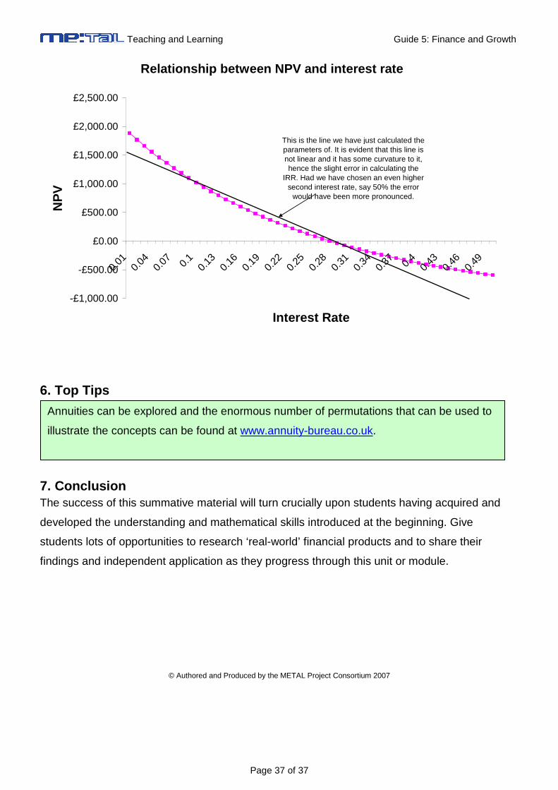
The graph below helps to illustrate the link between the interest rate and the NPV:


of 37

Relationship between NPV and interest rate

-£1,000.00

-£500.00

£0.00

£500.00

£1,000.00

£1,500.00

£2,000.00

£2,500.00

0.01

0.04

0.07 0.

10.

130.

160.

190.

220.

250.

280.

310.

340.

37 0.4

0.43

0.46

0.49

Interest Rate

NP

V

This is the line we have just calculated the parameters of. It is evident that this line is not linear and it has some curvature to it, hence the slight error in calculating the

IRR. Had we have chosen an even higher second interest rate, say 50% the error

would have been more pronounced.

6. Top Tips

7. Conclusion The success of this summative material will turn crucially upon students having acquired and

developed the understanding and mathematical skills introduced at the beginning. Give

students lots of opportunities to research ‘real-world’ financial products and to share their

findings and independent application as they progress through this unit or module.

© Authored and Produced by the METAL Project Consortium 2007

Annuities can be explored and the enormous number of permutations that can be used to

illustrate the concepts can be found at www.annuity-bureau.co.uk.

Finance and Growth - Mathematics for Economics: enhancing

Documents

Transcript of Finance and Growth - Mathematics for Economics: enhancing