
Final Thesis Report August - Repository Home
96
Abstract GHOSH, RAHUL. Error analysis of Through Reflect Line method for calibrating microwave measurements. (Under the direction of Professor Michael B. Steer) Uncertainty in transmission line based calibration techniques for microwave measurements are studied with the aim of identifying the optimum calibration conditions. Variation in the determined error parameters under certain conditions in Through Reflect Line (TRL) calibration method due to variation in the unknown reflection coefficient are analyzed experimentally and theoretically. It is found that measured uncertainty is minimized when the reflection standard is either a short or an open. The TRL calibration method is compared with the Through-Line (TL) calibration procedure. The major causes of uncertainties inherent in TRL calibration are absent in the TL calibration technique due to the synthesized reflection standard.
Transcript of Final Thesis Report August - Repository Home
Abstract
GHOSH, RAHUL. Error analysis of Through Reflect Line method for calibrating
microwave measurements. (Under the direction of Professor Michael B. Steer)
Uncertainty in transmission line based calibration techniques for microwave
measurements are studied with the aim of identifying the optimum calibration
conditions. Variation in the determined error parameters under certain conditions in
Through Reflect Line (TRL) calibration method due to variation in the unknown
reflection coefficient are analyzed experimentally and theoretically. It is found that
measured uncertainty is minimized when the reflection standard is either a short or an
open. The TRL calibration method is compared with the Through-Line (TL)
calibration procedure. The major causes of uncertainties inherent in TRL calibration
are absent in the TL calibration technique due to the synthesized reflection standard.
Error Analysis of the Through Reflect Line Method for Calibrating Microwave
Measurements
By
Rahul Ghosh
A thesis submitted to the Graduate Faculty of North Carolina State University
in partial fulfillment of the requirements for the Degree of
Master of Science
Electrical Engineering
Raleigh
2003 Approved by:- Prof. Gianluca Lazzi Prof. Griff Bilbro __________________________ _____________________________
Prof. Michael Steer, Chair of Advisory Committee
_____________________________________________________________________

ii
Biographical Summary
Rahul Ghosh was born on 8th January 1979 in Calcutta, India. He received his
elementary and secondary education in East Africa. He received the Bachelor of
Science degree with a major in Electronics from on The Pune University, India, in
2000. From July 2000 until July 2001 he completed the Post-Graduate Diploma
course in VLSI Design at Bitmapper Integration Technologies Pvt Ltd. In August
2001 he was admitted to North Carolina State University to study for the Master of
Science in Electrical Engineering. His interest is in the field of hardware design.

iii
Acknowledgements
I wish to express my appreciation to my advisor Dr. Michael Steer for his continuous
support, guidance and hours of in-depth discussion that made this work possible. I
would also like to thank Dr. Griff Bilbro and Dr. Gianluca Lazzi for serving on my
committee. I would like to express my appreciation to Mr. Jayesh Nath and Mr. Mark
Buff for their help and patience during the lengthy hours taking the measurements and
clearing my doubts. My special thanks go to all of my other friends for their moral
support and encouragement. And finally, I would like to express my gratitude to my
past and present instructors who taught me and who provided me useful information
about electrical engineering. This work is dedicated to my late father Aloy Kumar
Ghosh.
iv
Table of Contents List of Figures vi
1 Introduction 01
1.1 Motivation………………………………………………………………….. 01
1.2 Thesis Overview…………………………………………………………… 02
2 Literature Overview 03
2.1 Introduction to Smith Charts and VNA…………………….……………… 03
2.1.1 Microstrip Device Measurements………………………………….. 04
2.2 Measurement Errors ……………………………………………………...... 05
2.2.1 Error Correction Techniques……………………………………….. 05
2.3 Measurements Calibration Standards……………………………………….06
2.3.1 One port Calibration………………………………………………...06
2.3.2 Two Port Calibration………………………………………………. 08
2.3.2.1 SOLT Calibration………………………………………….. 09
2.3.2.2 TSD Calibration……………………………...…………….. 10
2.3.2.3 TRL Calibration……………………………………………. 10
2.3.2.4 LRM Calibration…………………………………………… 12
2.3.2.5 TL Calibration……………………………………………… 13
2.4 Conclusion…………………………………………………………………. 17
3 TRL Calibration 19
3.1 Steps in TRL Calibration………………………………………………….. 19
3.2 TRL De-Embedding Solution……………………………………………… 20
3.3 Limitations of TRL Calibration……………………………………………. 25
3.4 Conclusion…………………………………………………………………..26
4 Error Analysis of TRL Calibration 27
4.1 Proposed error in TRL calibration…………………………………………. 27
4.1.1 Analysis of the proposed inherent Error in TRL Calibration……..…. 31
4.2 Comparisons between TRL and TL Calibrations………………………….. 35
v
4.3 Conclusion…………………………………………………………………..39
5 Experimental Results 41
5.1 General Measurement Steps..…..………………………………………….. 41
5.2 Experiment Setup..……………..…………………………………………... 42
5.3 MATLAB Simulation Results…………………………………………….. 46
5.3.1 TRL Calibration results obtained from using short and open
standards…………………………………………………………… 46
5.3.1.1 TRL calibration for an air filled transmission line………… 50
5.3.1.2 TRL calibration for a 20dB attenuator…………………….. 53
5.3.1.3 TRL calibration for a combination of a 20 dB attenuator
and a transmission line……………………………………... 57
5.3.1.4 Comparison of results from TRL calibrations for the three
devices……………………………………………………... 60
5.3.2 TRL Calibration results obtained from using 20 dB
attenuator along with short and open standards……...……………. 60
5.3.2.1 TRL calibration for an air filled transmission line…………. 62
5.3.2.2 TRL calibration for a 20dB attenuator…………………….. 65
5.3.2.3 TRL calibration for a combination of a 20 dB attenuator
and a transmission line…………………………………….. 68
5.3.2.4 Comparison of results from TRL calibrations for the three
devices with the 20dB attenuator connected to the short
and open standard………………………………………….. 72
6 Conclusions 73
References 74
Appendix 76
A Detailed TRL De-Embedding Solution...…………………………………...76
B MATLAB Code for TRL De-embedding…………………………………...81
vi
List of Figures Figure 2.1: Reference planes in on-wafer microwave measurement ….. 04
Figure 2.2: One port OSL calibration standards ……...……………….. 07
Figure2.3: One port error model ……………………………………… 07
Figure 2.4: Two port forward error model …………………………….. 08
Figure 2.5: Modified eight term error model ………………………….. 11
Figure 2.6: Two port error model for asymmetric fixtures …………… 14
Figure 2.7: Reduced two port error model for symmetric fixtures …… 15
Figure 2.8: Signal flow graph of reduced two port error model for
Symmetric fixtures………………………………………… 16
Figure 2.9 Signal flow graph of ideal short as reflection
coefficient …………………………………………………. 17
Figure 3.1 Fictitious two port error boxes A, B with the three
Standards ………………………………………………….. 21
Figure 5.1 Reflection coefficients of the short standard ……………… 47
Figure 5.2 Reflection coefficients of the open standard ……………… 48
Figure 5.3 Reflection coefficients of the match standard …………….. 49
Figures 5.4-5.6 Calculated reflection coefficient from TRL algorithm for
air filled transmission line…………………………………. 50
Figure 5.7 Error factor for different standards used in TRL
procedure ….………………………………………………. 52
Figures 5.8-5.10 Calculated reflection coefficient from the TRL algorithm
for 20dB attenuator………………………………………… 54
Figure 5.11 Error factor for different standards used in TRL procedure
for the 20dB attenuator…………………………………….. 56
Figures 5.12-5.14 Calculated reflection coefficient from the TRL algorithm
for 20dB attenuator and air filled transmission line……….. 57
Figure 5.15 Error factor for different standards used in TRL procedure
for the 20dB attenuator and air filled transmission line…… 59
Figure 5.16 Reflection coefficients of the 20 dB attenuator and
open standard………………………………………………. 60
vii
Figure 5.17 Reflection coefficients of the 20 dB attenuator and
short standard……………………………………………… 61
Figures 5.18-5.20 Calculated reflection coefficient from the TRL algorithm
for airline………………………………………………….. 63
Figure 5.21 Error factor for different modified standards used in
TRL procedure for the airline……………………………… 65
Figures 5.22-5.24 Calculated reflection coefficient from the TRL algorithm
for 20dB attenuator with modified standards……………… 66
Figure 5.25 Error factor for different modified standards used in
TRL procedure for the 20dB attenuator……………………. 68
Figures 5.26-5.28 Calculated reflection coefficient from the TRL algorithm
for 20dB attenuator and air filled transmission line
with modified standards……………………………………. 69
Figure 5.29 Error factor for different modified standards used in
TRL procedure for the 20dB attenuator and airline……….. 70
1
Chapter 1: Introduction 1.1 Motivation
The main motivation for this work is the recent development of a new technique, the
Through Line (TL) calibration procedure developed by M. B. Steer, S. B. Goldberg,
G. Rinnet, P. D. Franzon, I. Turlik and J. S. Kasten [1]. Under certain conditions this
is a replacement for the Through-Reflect-Line (TRL) calibration procedure developed
by G.F. Engen and C.A. Hoer [2]. Even though TRL is the most widely used
calibration technique, this work tries to delve into the reasons why TL calibration
appears to have better characteristics than the TRL calibration technique. In
particular, the TRL procedure appears to have glitches when the length of the line
standard is close to integer multiple of a half wavelength. These glitches are not
apparent in TL calibration.
The TRL calibration technique suffers from inherent errors that result in
uncertainties in the measurement when the phase delay along the line is a multiple of
180 degrees. The TL calibration also suffers from this inherent problem, but the
reduced number of standards required in TL calibration is a major reason for better
results as compared to TRL calibration. The Reflect standard for the TRL calibration
need not be known accurately. This requirement makes the TRL calibration less
susceptible to errors as compared to other calibration techniques like Through Short
Delay (TSD) that requires the Reflection standard to be accurately known. This still
does not guarantee that the TRL procedure is error free. In this work an error factor
inherent in TRL calibration that is absent in TL calibration is found.
2
1.2 Thesis Overview
Chapter 2 presents a literature overview including brief introduction to the need for
calibration in the microwave measurement. The basic operating principle of a vector
network analyzer is discussed along with the different terminology associated with
network analysis. Different types of errors and techniques of error correction applied
to network analyzer measurements are discussed. The different error correcting
calibration techniques are explained along with their inherent drawbacks and
advantages. Chapter 3 discusses the TRL calibration procedure in detail as this
calibration is the most popular and widely used for on-wafer measurements. The
inherent errors in TRL calibration are discussed in details. Next the new calibration
technique, TL calibration, is introduced and comparisons are made between the TRL
and TL calibration methods. Chapter 4 discusses another possible inherent error, the
variation in the reflection coefficient standard seen at the two ports of network
analyzer that causes variation in the measured parameters for the error boxes in the
TRL calibration and considerations to be made in selecting the Reflection standard to
minimize these variations. Chapter 5 presents the experimental verification for the
proposed error present in TRL. This includes MATLAB code implementing the TRL
algorithm and the inherent errors introduced for different reflection co-efficient
standards.
3
Chapter 2: Literature Review 2.1 Introduction to Smith Charts and VNA
This section gives an overview of the fundamental principles of vector network
analysis and Smith Charts [7]. Network analyzers accurately measure ratios of the
incident, reflected, and transmitted energy, e.g., the energy that is launched onto a
transmission line, reflected back down the transmission line toward the source (due to
impedances mismatch), and successfully transmitted to the terminating device. The
amount of reflection that occurs when characterizing a device depends on the
impedance that the incident signal “sees”. This impedance can be represented by real
and imaginary parts. Instead of plotting impedance directly, the complex reflection
coefficient is displayed in vector form. The magnitude of the vector is the distance
from the center of the display, and phase is displayed as the angle of vector referenced
to a flat line from the center to the right-most edge. Smith charts are normally to
represent this.
As mentioned in [8], Smith Chart is a polar plot of the complex reflection
coefficient or also known as the 1-port scattering parameter 11S , for reflections from a
normalized complex load impedance; the normalized impedance is a complex
dimensionless quantity obtained by dividing the actual load impedance ZL in ohms by
the characteristic impedance Zo (also in ohms, and a real quantity for a lossless line) of
the transmission line. On the Smith Chart, loci of constant resistance appear as circles,
while loci of constant reactance appear as arcs. Impedances on the Smith chart are
always normalized to the characteristic impedance of the component or system of
interest, usually 50 ohms for RF and microwave systems and 75 ohms for broadcast
4
and cable-television systems. A perfect termination appears in the center of the Smith
chart.
2.1.1 Micro-strip device measurements
Microstrip devices cannot be connected directly to the coaxial ports of a network
analyzer. The device under test (DUT) must be physically connected to the network
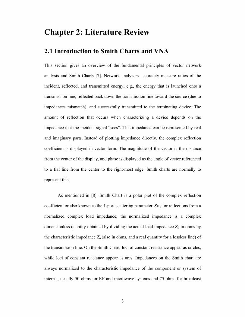
analyzer by some kind of transition network or fixture. The Figure 2.1 below shows a
typical block diagram of the different reference planes in microstrip device
measurement.
In order to get the accurate measurement we need to remove all errors up to
the fixture reference plane. This means that the internal Vector Network Analyzer
(VNA) as well as coaxial cable errors must be removed. Calibration for a fixture
measurement in micro-strip presents additional difficulties.
On-wafer Reference Plane
VNA and
Cable Errors
FIXTURE ERRORS
FIXTURE ERRORS
VNA and
Cable Errors
DUT
-------------- Co-axial Reference Plane --------------
Figure 2.1: Reference planes in on-wafer microwave measurement.
Calibration at the coaxial ports of the network analyzer removes the effects of
the network analyzer and any cables or adapters before the fixture; however, the

5
effects of the fixtures themselves are not accounted for. Thus calibration standards are
required at the probe tips.
2.2 Measurement Errors
Errors in network analyzer measurements can be separated into three categories [9]:
1) Systematic errors are the most significant source of measurement uncertainty
in RF and Microwave measurements, caused by imperfections in the test equipment
and test setup. These errors can be characterized through calibration and
mathematically removed during the measurement process. Systematic errors
encountered in network measurements are related to signal leakage, signal reflections,
and frequency response. The six systematic errors in the forward direction are
directivity, source match, reflection tracking, load match, transmission tracking, and
isolation. The reverse error model is a mirror image, giving a total of 12 error terms
for two-port measurements.
2) Drift errors occur when a test system’s performance changes after a
calibration has been performed. They are primarily caused by temperature variation
and can be removed by additional calibration.
3) Random errors vary as a function of time. Since they are not predictable they
cannot be removed by calibration. The main contributors to random errors are
instrument noise, switch repeatability, and connector repeatability.
2.2.1 Error Correction Techniques
Vector error correction [9] is the most widely used approach to removing systematic
errors. This type of error correction requires a network analyzer capable of measuring

6
phase as well as magnitude, and a set of calibration standards with known, precise
electrical characteristics. The vector-correction process characterizes systematic error
terms by measuring known calibration standards, storing these measurements within
the analyzer’s or controller’s memory, and using this data to calculate an error model
which is then used to remove the effects of systematic errors from subsequent
measurements. This calibration process accounts for all major sources of systematic
errors and permits very accurate measurements. However, measurement accuracy is
largely dependent upon calibration standards, and a set of calibration standards is
often supplied as a calibration kit.
2.3 Measurement Calibration Standards
The two main types of vector error correction are the one-port and two-port
calibrations.
2.3.1 One Port Calibration
This procedure consists of measuring a series of known calibration standards. Based
on the measurements of these known standards, an error model of the performance
characteristics of the microwave hardware internal to the network analyzer can be
constructed. After this error model has been generated from the measurement of the
calibration standards, the network analyzer removes the systematic errors from the
other devices.
7
SHORT OPEN LOAD
DUT
Figure 2.2: One port OSL calibration standards.
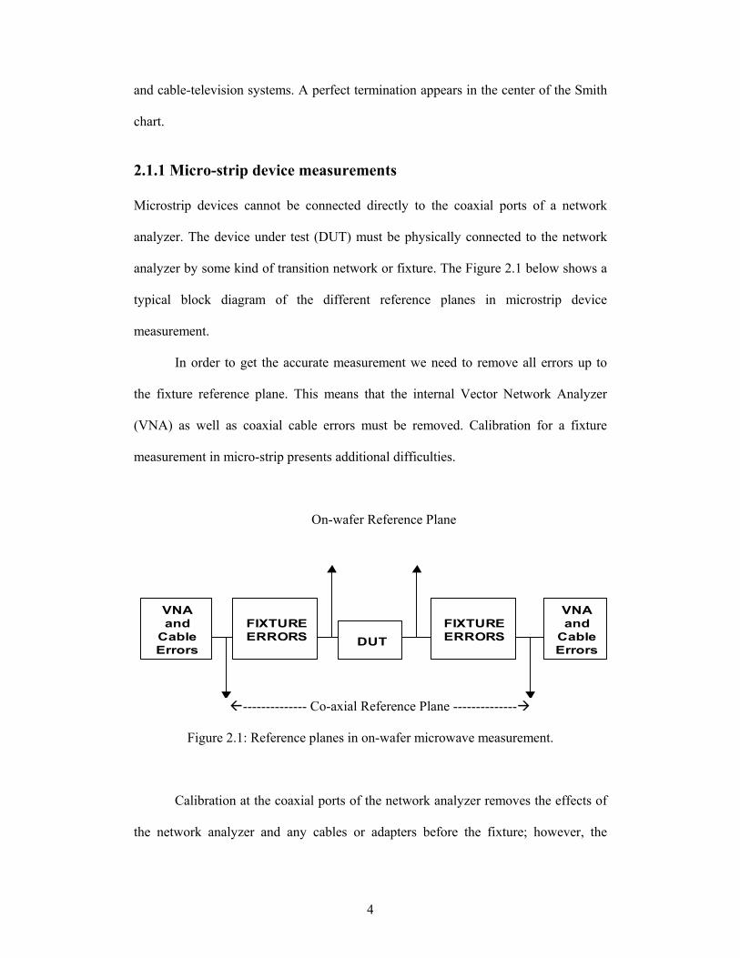
The three standards used for 1-port calibration are the short, open, and
matched termination as shown in Figure 2.2. Based on the measurements made for
each of these standards, the values of the components in the systematic error model
(e00, e01 and e11), as shown in Figure 2.3, can be computed. Once these values are
found, the S parameters of the DUT can be corrected for these non-idealities.
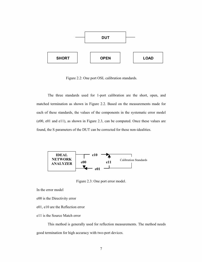
Figure 2.3: One port error model.
In the error model
e00 is the Directivity error
e01, e10 are the Reflection error
e11 is the Source Match error
This method is generally used for reflection measurements. The method needs
good termination for high accuracy with two-port devices.
IDEAL NETWORK ANALYZER e00 e11
e01
e10Calibration Standards
8
2.3.2 Two Port Calibration
In calibrating a two-port device however, one port calibration assumes a good
termination on the unused port of the DUT. This may cause inaccuracies if the unused
port of the DUT is not perfectly matched. To obtain highest accuracy two-port error
correction is used. The two-port error correction yields the most accurate results
because it account for all of the major sources of systematic error. The error model
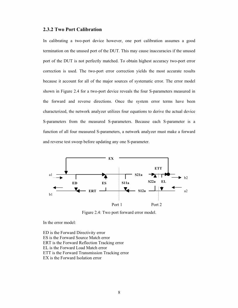
shown in Figure 2.4 for a two-port device reveals the four S-parameters measured in
the forward and reverse directions. Once the system error terms have been
characterized, the network analyzer utilizes four equations to derive the actual device
S-parameters from the measured S-parameters. Because each S-parameter is a
function of all four measured S-parameters, a network analyzer must make a forward
and reverse test sweep before updating any one S-parameter.
Figure 2.4: Two port forward error model.
In the error model:
ED is the Forward Directivity error ES is the Forward Source Match error ERT is the Forward Reflection Tracking error EL is the Forward Load Match error ETT is the Forward Transmission Tracking error EX is the Forward Isolation error
S11a S22a
S12a
ED ES
ERT
Port 1 Port 2
EX
S21a
EL
a1
b1
b2
a2
ETT
9
The most commonly used two-port calibration techniques are:
Short Open Load Through (SOLT)
Through Short Delay (TSD)
Through Reflect Line (TRL)
Line Reflect Match (LRM)
And Through Line (TL)
These calibration techniques are described in the sections below.
2.3.2.1 Short Open Load Through (SOLT) Calibration
Calibration at the coaxial ports of the network analyzer removes the effect of the
network analyzer and any other cable before the fixture. Most network analyzers
already contain standard calibration kit definition files that describe the characteristics
of a variety of calibration standards. These calibration kit definitions usually cover the
major types of coaxial connectors used for component and circuit measurements.
This method is simpler and very accurate as long as the standards are accurately
defined.
The SOLT calibration technique is often preferred when S-parameters are
measured with respect to an ideal characteristic impedance such as 50 ohm. Main
characteristics of Short Open Load Though Calibration are that all standards open,
short, load must be perfectly known. The open standard is typically realized as an
unterminated transmission line. Electrical definition of an ideal open has unity
reflection with no phase shift. The actual model for the open, however, does have
some phase shift due to fringing capacitance. The electrical definition of an ideal short
is unity reflection with 180 degrees of phase shift. All of the incident energy is
reflected back to the source, perfectly out of phase with the reference. A simple short
10
circuit from a single conductor to ground makes a good short standard. For example,
the short can be vias (plated through holes) to ground at the end of a micro-strip
transmission line. If coplanar transmission lines are used, the short should go to both
ground planes. To reduce the inductance of the short, avoid excessive length. A good
RF ground should be near the signal trace. An ideal load reflects none of the incident
signal, thereby providing a perfect termination over a broad frequency range. We can
only approximate an ideal load with a real termination because some reflection always
occurs at some frequency, especially with non-coaxial actual standards.
2.3.2.2 Through Short Delay (TSD) calibration
TSD was developed by N. R. Franzen and R. A. Spaciale [11] and is based on both
reflection and transmission measurements and it offers two advantages. First, a
matched load standard in not required and second it uses mechanically simple
standards. TSD is not without disadvantage. The delay standard is assumed lossless
and nonreflecting i.e. the propagation constant was pure delay and the impedance was
the measurement system or 50 ohms. Also, TSD requires information from two
delays; the through connection and the actual delay. If the phase difference between
these two is near zero or 180 degrees the algorithm fails to return a valid result. This
is a limitation of any de-embedding technique using a delay type standard.
2.3.2.3 Through Reflect Line (TRL) Calibration
For in-fixture calibration high quality Short-Open-Load-Thru (SOLT) standards are
not readily available for full 2-port calibration of the system at the desired
measurement plane of the device. In microstrip, a practical short circuit or via is
inductive, a practical open circuit radiates energy and a high-quality purely resistive
11
load is difficult to produce over a broad frequency range. TRL Calibration as
developed by Engen and Hoer [1], used only one delay standard with a through
connection and an arbitrary reflection to calibrate their network analyzer. The delay
standard could be arbitrary, with its propagation constant unknown, however, the line
was assumed nonreflecting. The reflection standard could be any repeatable reflecting
load and they suggested either an open or short circuit. The Through Reflect Line
(TRL) 2-port calibration is an alternative to the traditional SOLT full 2-port
calibration technique that utilizes simpler more convenient standards, for device
measurements in the microstrip environment.
The TRL method is more suitable for obtaining S-parameters with respect to
the impedance of on wafer transmission lines. When accurate on-wafer Line standards
are available, the TRL method usually offers better accuracy than the SOLT
technique. A TRL 2-port calibration kit uses at least three standards to define the
calibrated reference plane. For TRL two port calibrations, the 12 terms error model as
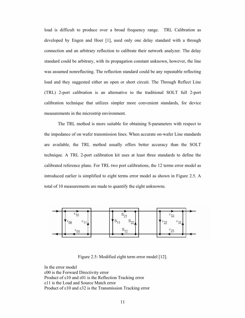
introduced earlier is simplified to eight terms error model as shown in Figure 2.5. A
total of 10 measurements are made to quantify the eight unknowns.
Figure 2.5: Modified eight term error model [12].
In the error model ε00 is the Forward Directivity error Product of ε10 and ε01 is the Reflection Tracking error ε11 is the Load and Source Match error Product of ε10 and ε32 is the Transmission Tracking error
12
An assumption is made that:
ε11 = Forward Source Match error = Reverse Load Match error.
ε22 = Reverse Source Match error = Forward Load Match error.
The main characteristic of Though Reflect Line Calibration are that the TRL
technique requires only a through-line (Through) and a transmission line offset (Line)
as references. The TRL method also employs highly reflecting impedances (Reflects)
as standards, but their exact electrical characteristics are not required. However,
Reflect standards must be accurately repeated at each test port. The TRL calibration
uses the characteristic impedance of the length of the transmission line standard to set
the reference impedance. This approach restricts the range of frequency that can be
measured as the insertion phase of the line should lie between 20 and 160 degrees.
Because of this reason, most of the Line standards can only be used over an 8:l
frequency range. For broadband measurements several Line standards may be
required. At low frequencies, Line standards can become inconveniently long.
Another concern is the change of the reference impedance due to the effects of loss
and dispersion in the TRL Line standards. The accuracy of the method depends on the
estimate of the characteristic impedance of the Line standard.
2.3.2.4 Load Reflect Match (LRM) Calibration
The standards for the LRM calibration method are a non-zero length Through line, a
Reflect and a Match. The LRM calibration method is similar to the TRL calibration
method, except that a perfect match on each port is substituted in place of the Line
standard. The matched standard can be seen as an infinitely long line. The LRM
13
reflect is the same as the TRL reflect standard, the value of the reflection standard
need not be known accurately, but must be the same for each port. The LRM Line
standard corresponds to the TRL Through standard.
The LRM calibration offers a number of advantages. Firstly, the Matched
standard is the only impedance that needs to be accurately known thereby reducing
the errors caused by improperly defined open or short standards used in SOLT
calibration method. The advantage over the SOLT calibration lies in the fact that
LRM calibration uses lesser standards that results in fewer standard definitions and
the errors resulting from imperfect standard definition are minimized. Secondly, the
use of Matched standard to determine the reference impedance reduces the variation
in the reference impedance value as observed in TRL method and enables broadband
frequency coverage.
2.3.2.5 Through Line Calibration
The Through Line (TL) calibration is a two tier calibration procedure. The TL method
utilizes measurements of the through and line following approximate Open Short Line
calibration. The Through Line calibration is implemented in three steps. The first step
is to apply Open Short Load (OSL) calibration to each of the two test ports. The only
requirement for the OSL calibration is that the same reference impedance be used at
the two test ports. The second step is to perform the through and line measurements.
The through measurement yields the reflection coefficient of an ideal short placed at
the fixture reference plane. This removes the need for arbitrary reflection standard as
in TRL procedure thus removing the major source of ambiguity.
14
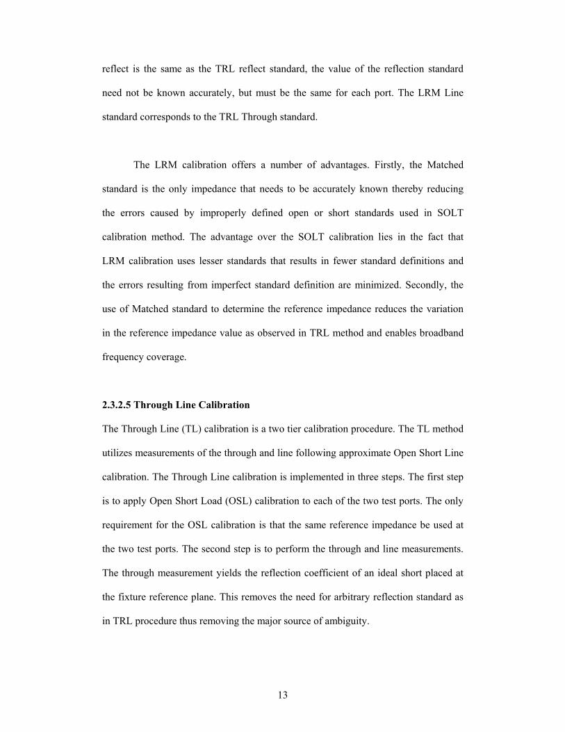
Figure 2.6 below shows the conventional two port error network and its
corresponding signal flow graph. It is composed of two error networks A and B where
the individual signal paths Sija and Sijb are unique forcing the fixture S parameters Sijf
to be unequal to each other. This represents an asymmetric fixture. As explained in
[13], the fixture is symmetric if the port 1 and 2 reflection coefficients are equal and
the fixture is reciprocal, i.e. if S11f = S22f and S21f = S12f. Reciprocity is true when the
fixture is passive and non-magnetic and these symmetrical equalities are possible with
two orders of symmetry; first and second order.
Figure 2.6: Two port error model for asymmetric fixtures [13].
From the signal flow graph of the asymmetric fixtures in Figure 2.6, applying
Mason’s rule yields
S11f = S11a +11b22a
11b12a21a
SS-1SSS (2.1)
S22f = S22b +11b22a
12b21b22a
SS-1SSS (2.2)
S21f = 11b22a
21b21a
SS-1SS (2.3)
15
And
S12f = 11b22a
12b12a
SS-1SS (2.4)
From equation 2.1 and 2.2 we get
S11a (1- S22aS11b) + S11b S221a = S22b (1- S22aS11b) + S11b S2
21a (2.5)
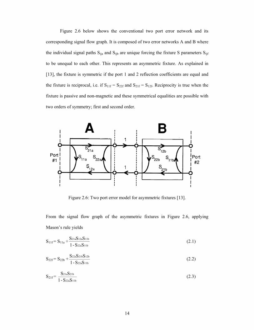
As a result of approximate OSL calibration, the calibrated fixtures of the test system
are identical. Hence in a through connection the embedded device under test is
symmetrical. Symmetry permits the synthesis of TRL reflection standards. A first-
order symmetric fixture has identical fixture halves that are symmetric as shown in
Figure 2.7. The port two error network, B, is now a port reverse of A, or B = AR. This
is true if Slla = S22b, S22a = Sllb. Moreover, these conditions satisfy the symmetry
condition equation (2.5). Most importantly, the signal flow graph in Figure 2.8 shows
symmetry reduces the number of error terms to three, the A network only. In other
words, symmetry reduces the number of error terms for a two port fixture.
Figure 2.7: Reduced two port error model for symmetric fixtures [13].
16
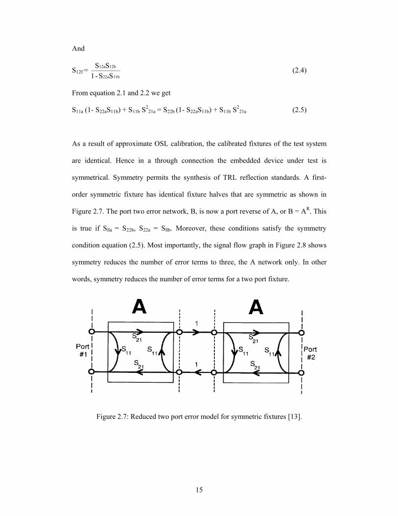
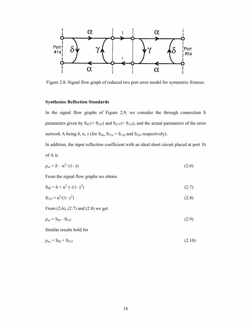
Figure 2.8: Signal flow graph of reduced two port error model for symmetric fixtures.
Synthesize Reflection Standards
In the signal flow graphs of Figure 2.9, we consider the through connection S
parameters given by Sllf (= S22f) and S21f (= S12f), and the actual parameters of the error
network A being δ, α, γ (for Slla, S21a = S12a and S22a respectively).
In addition, the input reflection coefficient with an ideal short circuit placed at port 1b
of A is
ρsc = δ – α2/ (1- γ) (2.6)
From the signal flow graphs we obtain
Sllf = δ + α2 γ /(1- γ2) (2.7)
S21f = α2/(1- γ2) (2.8)
From (2.6), (2.7) and (2.8) we get
ρsc = Sllf - S21f (2.9)
Similar results hold for
ρoc = Sllf + S21f (2.10)
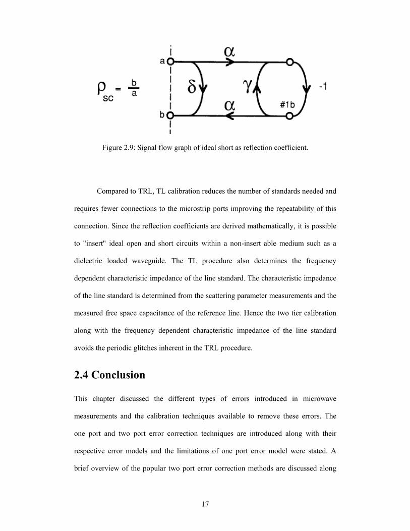
17
Figure 2.9: Signal flow graph of ideal short as reflection coefficient.
Compared to TRL, TL calibration reduces the number of standards needed and
requires fewer connections to the microstrip ports improving the repeatability of this
connection. Since the reflection coefficients are derived mathematically, it is possible
to "insert" ideal open and short circuits within a non-insert able medium such as a
dielectric loaded waveguide. The TL procedure also determines the frequency
dependent characteristic impedance of the line standard. The characteristic impedance
of the line standard is determined from the scattering parameter measurements and the
measured free space capacitance of the reference line. Hence the two tier calibration
along with the frequency dependent characteristic impedance of the line standard
avoids the periodic glitches inherent in the TRL procedure.
2.4 Conclusion
This chapter discussed the different types of errors introduced in microwave
measurements and the calibration techniques available to remove these errors. The
one port and two port error correction techniques are introduced along with their
respective error models and the limitations of one port error model were stated. A
brief overview of the popular two port error correction methods are discussed along

18
with their advantages and disadvantages. In the next chapter the Through Reflect Line
calibration is discussed in detail along with the derivation of the TRL algorithm.
19
Chapter 3: TRL Calibration
This chapter discusses the TRL calibration technique [3] in depth and analyzes the
different steps involved in this calibration and why this method is the most popular of
all. The inherent advantage of TRL calibration as compared to all other calibration
techniques discussed so far is that the value of the reflection standard need not be
known. The main features of TRL calibration have already been discussed in the
previous chapter. In this chapter the mathematical analysis of the TRL deembedding
procedure is presented as this is necessary to understand the proposed inherent error
introduced due to the arbitrary reflection coefficient.
3.1 Steps in TRL Calibration For the ‘thru’ step, the test ports are connected together directly (zero length thru) or
with a short length of transmission line (non-zero length thru). The transmission
frequency response and port match are measured in both directions by measuring all
four S-parameters. For the ‘reflect’ step, identical high reflection coefficient standards
(typically open or short circuits) are connected to each test port and measured ( 11S
and 22S ). For the ‘line’ step, a short length of transmission line different in length
from the THRU) is inserted between port 1 and port 2 and again the frequency
response and port match are measured in both directions by measuring all four S-
parameters. In total, ten measurements are made, resulting in ten independent
equations. However, the TRL error model has only eight error terms to solve for. The
‘reflect’ standard and the propagation constant of the ‘line’ standard are determined.
Because these terms are solved for, they do not have to be specified initially. The
20
characteristic impedance of the ‘line’ standard becomes the measurement reference
and, therefore, has to be assumed ideal (or known and defined precisely).
3.2 TRL De-Embedding Solution
The basic TRL calibration outlined in [1] is based on the eight term error model. The
procedure then consists of finding the S parameters for the two two-port error
matrices. A more detailed derivation of the TRL calibration equations is given in
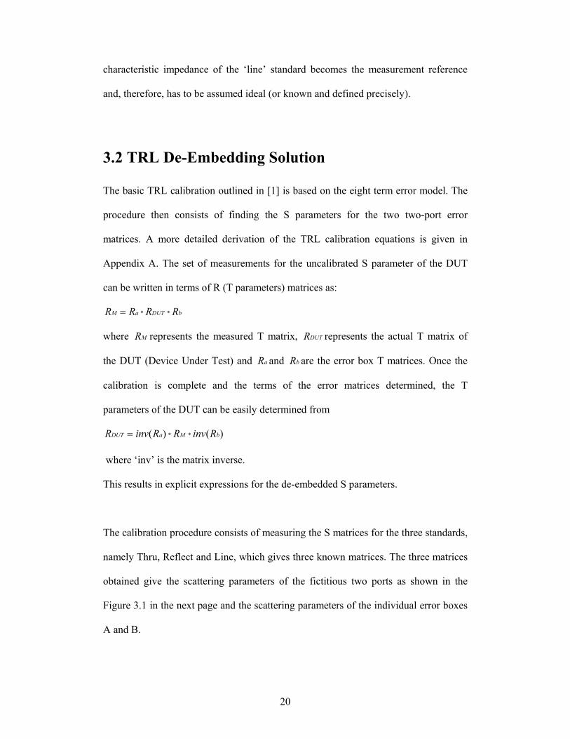
Appendix A. The set of measurements for the uncalibrated S parameter of the DUT
can be written in terms of R (T parameters) matrices as:
bDUTaM RRRR **=
where MR represents the measured T matrix, DUTR represents the actual T matrix of
the DUT (Device Under Test) and aR and bR are the error box T matrices. Once the
calibration is complete and the terms of the error matrices determined, the T
parameters of the DUT can be easily determined from
)()( ** bMaDUT RinvRRinvR =
where ‘inv’ is the matrix inverse.
This results in explicit expressions for the de-embedded S parameters.
The calibration procedure consists of measuring the S matrices for the three standards,
namely Thru, Reflect and Line, which gives three known matrices. The three matrices
obtained give the scattering parameters of the fictitious two ports as shown in the
Figure 3.1 in the next page and the scattering parameters of the individual error boxes
A and B.

21
Figure 3.1: Fictitious two-port error boxes A, B with the three standards. [3]
The emergent wave amplitudes b1, b2 at ports 1 and 2 are related to the incident
waves a1, a2 by the well-known scattering equations:
2121111 bSaSb += (3.1)
2221212 bSaSb += (3.2)
where the ijS are the scattering coefficients.
Dividing the first of these by al, the second by a2, and then eliminating the ratio al /a2
between them yields:
21222112 wwSwSw =∆−+ (3.3)
where
21122211 SSSS −=∆ (3.4)
Equation (3.5) shows the conversion between the T and the S parameters.
21
11
RR
22
12
RR
=
−
−−
21
22
21
11122211
SS
SSSSS
21
21
11
1S
SS
(3.5)
First convert the measured S parameters to their equivalent T parameters as in
Equation (3.5). Let the cascading matrix be represented by the matrix R. Let the

22
cascading matrices of the error two-ports A and B be denoted by Ra and Rb
respectively, while Rt represents their cascade ‘thru’ connection and Rd represents the
cascade ‘Line’ measurements and Rl1 represents the cascade matrix of the inserted
line.
The T matrix for the Though connection can be represented by
bat RRR = (3.6)
while the T matrix for the line connection can be represented by
blad RRRR 1= (3.7)
where
Ra matrix be represented by: Ra =
22a21a
12a11a
r rr r
or Ra = ar 22
ca
1b
aa rra 2211 /= , aa rrb 2212 /= and aa rrc 2221 /= .
Rb matrix be represented by: Rb =
22b21b
12b11b
r rr r
or Rb = br22
1
γ
βα
bb rr 2211 /=α , bb rr 2212 /=β and bb rr 2221 /=γ .
Solving equation (3.6) for Rb and substituting into equation (3.7) gives
2laa RRTR = where dRT = tR -1 (3.9)
The equation (3.9) consists of four equations with five unknowns. However there are
only three independent solutions to Equation (3.9). These solutions give
=ca / )/( 2111 aa rr , =b )/( 2212 aa rr

23
and e exp ( lγ2 ) = aaaa
aaaa
trrttrrt
11112112
22221221
)/()/(++ . (3.10)
Up to this step we have solved for two terms of the error matrix A and the
propagation constant of the transmission line. Using this information we can solve for
Rb using equation (3.6) to obtain two parameters of the error matrix B
namely αβ / andγ .
Next we make use of the reflection standard. The reflection coefficient measured at
port 1, 1w , can be written as a function of the reflection coefficient of the termination
lΓ and the S parameters of the error box A as
1w = 1+Γ
+Γl
l
cba (3.24)
or
a = )/1( *1
1
acwbw
l −Γ− (3.25)
Similarly, we can write for the measured reflection coefficient at the error box B as
2w = 1+Γ−
−Γl
l
βγα (3.26)
or
α =)/1( *2
2
αβγ
ww
l +Γ− . (3.27)
The unknown reflection coefficient lΓ is eliminated from Equation (3.25) and (3.27)
to yield
)]/1)(//[()])(/1)([( 221 aecacwbfdwbwa −+−+−±= γαβ (3.28)
Thus the need for the value of reflection coefficient to be exactly known is eliminated.
Once the value for ‘a’ for two port error matrix A is found, the remaining parameters
of the error matrix A and B can be easily found as
24
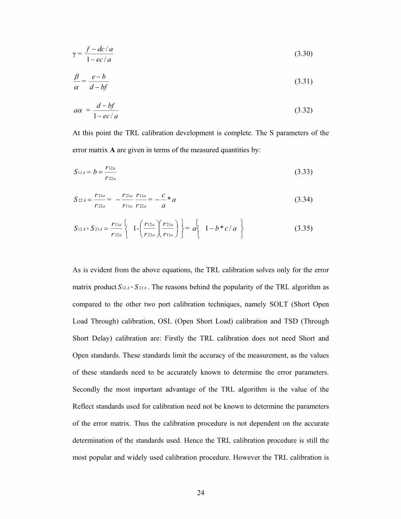
γ = aecadcf
/1/
−− (3.30)
αβ =
bfdbe
−− (3.31)
αa = aec
bfd/1−
− (3.32)
At this point the TRL calibration development is complete. The S parameters of the
error matrix A are given in terms of the measured quantities by:
=AS11a
a
rrb
22
12= (3.33)
=AS 22a
a
rr
22
21 = a
a
rr
11
21−
a
a
rr
22
11 = aac *− (3.34)
=AA SS 21*12a
a
rr
22
11
1-
a
a
a
a
rr
rr
11
21
22
12 = a 1
− acb /* (3.35)
As is evident from the above equations, the TRL calibration solves only for the error
matrix product AA SS 21*12 . The reasons behind the popularity of the TRL algorithm as
compared to the other two port calibration techniques, namely SOLT (Short Open
Load Through) calibration, OSL (Open Short Load) calibration and TSD (Through
Short Delay) calibration are: Firstly the TRL calibration does not need Short and
Open standards. These standards limit the accuracy of the measurement, as the values
of these standards need to be accurately known to determine the error parameters.
Secondly the most important advantage of the TRL algorithm is the value of the
Reflect standards used for calibration need not be known to determine the parameters
of the error matrix. Thus the calibration procedure is not dependent on the accurate
determination of the standards used. Hence the TRL calibration procedure is still the
most popular and widely used calibration procedure. However the TRL calibration is
25
not without its drawbacks. In the following section some of the drawbacks of the TRL
calibration procedure are discussed.
3.3 Limitations of Thru-reflect line (TRL) Calibration
The major limitation of the TRL technique is the limited bandwidth of Line standards.
Most Line standards can only be used over a limited frequency range. For broadband
measurements, several Line standards may be required. At low frequencies, Line
standards can become inconveniently long.
The algorithm requires the characteristic impedance of the line standard be
equal to the measurement system impedance. If not, its value has to be determined.
Also, the algorithm assumes real characteristic impedance with no frequency
dependence. If the fixture to be calibrated is composed of dispersive transmission
lines, e.g. microstrip, it becomes necessary to determine the complex characteristic
impedance as a function of frequency.
The insertion phase of the line must not be same as the thru (for zero or non-
zero length). This puts an important requirement that the difference between the
length of the Line standard (say l2 and the length of the thru standard (say l1 must be
between (20º and 160º) ± n×180º. Ideally the difference between the lengths is taken
to be ¼ wavelength or 90º of the insertion phase relative to the thru at the middle of
the desired frequency span. Hence the range of frequencies over which the
measurements are to be taken decides the center frequency, which in turn decides the
difference between the two lengths.

26
3.4 Conclusion
This chapter discussed in detail the TRL calibration procedure. The discussion
included the requirements of the standards used in the TRL calibration, the
mathematical analysis of the TRL de-embedding algorithm, the advantages of this
calibration procedure as compared to the other two port calibration methods. In the
end the inherent drawbacks and limitations of this popular procedure are discussed.
27
Chapter 4: Error Analysis of TRL Calibration
This chapter presents the reader with the new work done to investigate why the TL
(Through Line) calibration, under certain conditions provides a better alternative to
the TRL (Through Reflect Line) calibration. In the following sections the
discrepancies introduced in the calculated parameters of the error matrices due to the
arbitrary reflection standard is derived. The inherent assumption about the reflection
standard value in the TRL de-embedding algorithm is seen to cause variations in the
obtained parameters of the error matrices. From the derivation of this error factor, the
uncertainties are found to be dependent on the value of the selected arbitrary
reflection standard. Another phenomenon, namely the discrepancies in measurement
when the line difference approaches an integer multiple of a half wavelengths, is also
observed in TL calibration technique. Mathematical analysis is presented to indicate
the cause of these discrepancies in the TL and TRL calibration and the conclusion is
drawn that the discrepancies will be observed in all calibration procedure that uses the
through and delay standards as part of the calibration procedure.
4.1 Proposed Error in TRL calibration
There have been a number of papers investigating the various causes of error inherent
in TRL calibration. Marks [16] uses least mean square estimate and redundant
transmission line standards to minimize the effects of random errors introduced by
imperfect connector repeatability. The measured model in this paper is represented by
cascade of the fixture error matrices and the transmission line matrix. The fixtures
28
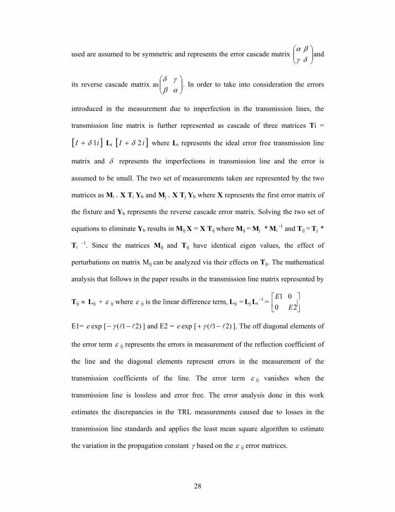
used are assumed to be symmetric and represents the error cascade matrix
γα
δβ
and
its reverse cascade matrix as
βδ
αγ
. In order to take into consideration the errors
introduced in the measurement due to imperfection in the transmission lines, the
transmission line matrix is further represented as cascade of three matrices Ti =
[ ]iI 1δ+ Li [ ]iI 2δ+ where Li represents the ideal error free transmission line
matrix and δ represents the imperfections in transmission line and the error is
assumed to be small. The two set of measurements taken are represented by the two
matrices as Mi = X Ti Yb and Mj = X Tj Yb where X represents the first error matrix of
the fixture and Yb represents the reverse cascade error matrix. Solving the two set of
equations to eliminate Yb results in Mij X = X Tij where Mij = Mj * Mi -1 and Tij = Tj *
Ti –1. Since the matrices Mij and Tij have identical eigen values, the effect of
perturbations on matrix Mij can be analyzed via their effects on Tij. The mathematical
analysis that follows in the paper results in the transmission line matrix represented by
Tij ≈ Lij + ε ij where ε ij is the linear difference term, Lij = Lj Li -1 =
0
1E
2
0E
E1= e exp [ )21( ll −− γ ] and E2 = e exp [ )21( ll −+ γ ]. The off diagonal elements of
the error term ε ij represents the errors in measurement of the reflection coefficient of
the line and the diagonal elements represent errors in the measurement of the
transmission coefficients of the line. The error term ε ij vanishes when the
transmission line is lossless and error free. The error analysis done in this work
estimates the discrepancies in the TRL measurements caused due to losses in the
transmission line standards and applies the least mean square algorithm to estimate
the variation in the propagation constant γ based on the ε ij error matrices.
29
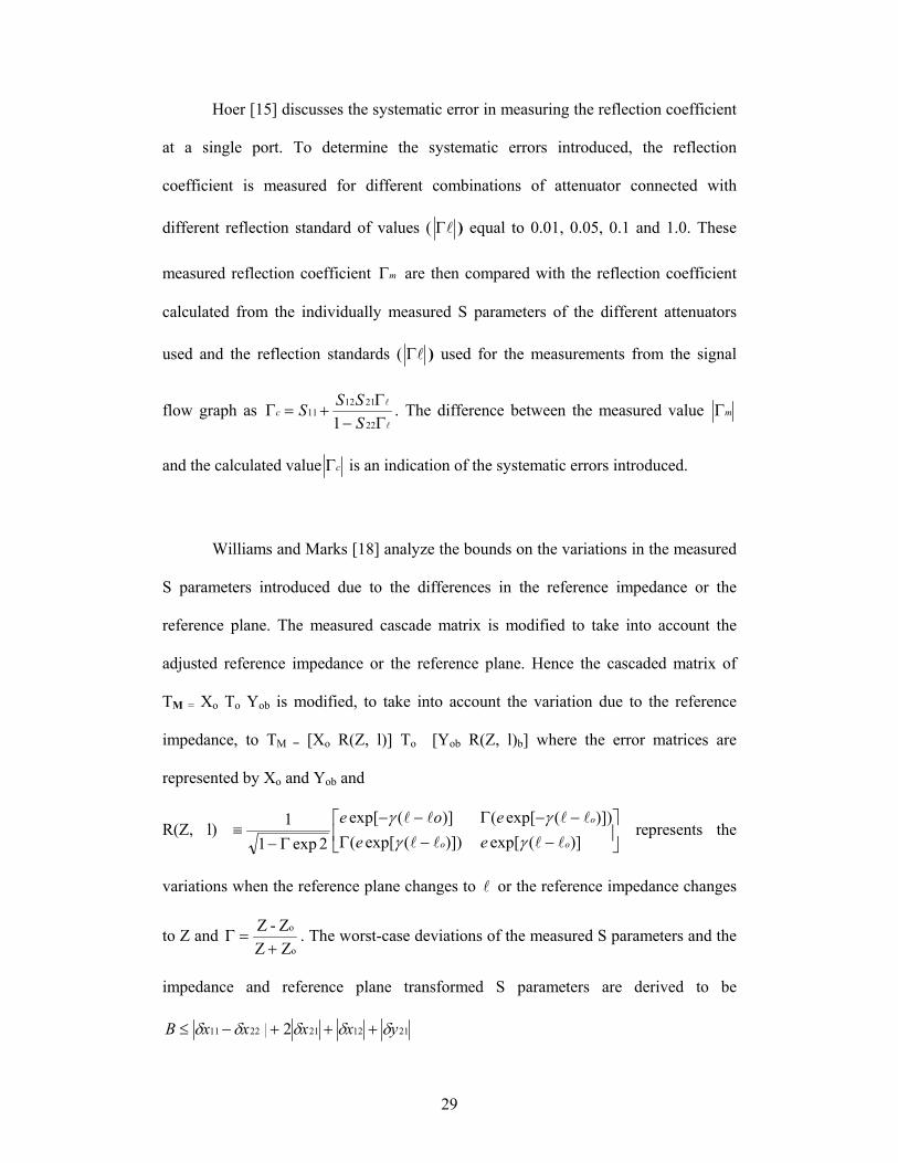
Hoer [15] discusses the systematic error in measuring the reflection coefficient
at a single port. To determine the systematic errors introduced, the reflection
coefficient is measured for different combinations of attenuator connected with
different reflection standard of values ( lΓ ) equal to 0.01, 0.05, 0.1 and 1.0. These
measured reflection coefficient mΓ are then compared with the reflection coefficient
calculated from the individually measured S parameters of the different attenuators
used and the reflection standards ( lΓ ) used for the measurements from the signal
flow graph as l
l
Γ−Γ
+=Γ22
211211
1 SSSSc . The difference between the measured value mΓ
and the calculated value cΓ is an indication of the systematic errors introduced.
Williams and Marks [18] analyze the bounds on the variations in the measured
S parameters introduced due to the differences in the reference impedance or the
reference plane. The measured cascade matrix is modified to take into account the
adjusted reference impedance or the reference plane. Hence the cascaded matrix of
TM = Xo To Yob is modified, to take into account the variation due to the reference
impedance, to TM = [Xo R(Z, l)] To [Yob R(Z, l)b] where the error matrices are
represented by Xo and Yob and
R(Z, l)
−Γ−−
Γ−≡
)])(exp[()](exp[
2exp11
oeoell
ll
γγ
−
−−Γ)](exp[
)])(exp[(o
o
ee
ll
ll
γγ
represents the
variations when the reference plane changes to l or the reference impedance changes
to Z and o
o
ZZZ-Z
+=Γ . The worst-case deviations of the measured S parameters and the
impedance and reference plane transformed S parameters are derived to be
2112212211 2 yxxxxB δδδδδ +++−≤
30
where I-l)] (Z, R [Xo=xδ and I-l)] (Z, R [Yo=yδ . This result shows the variation
between the measured and the actual S parameters of the DUT for change in the
reference impedance or the reference plane.
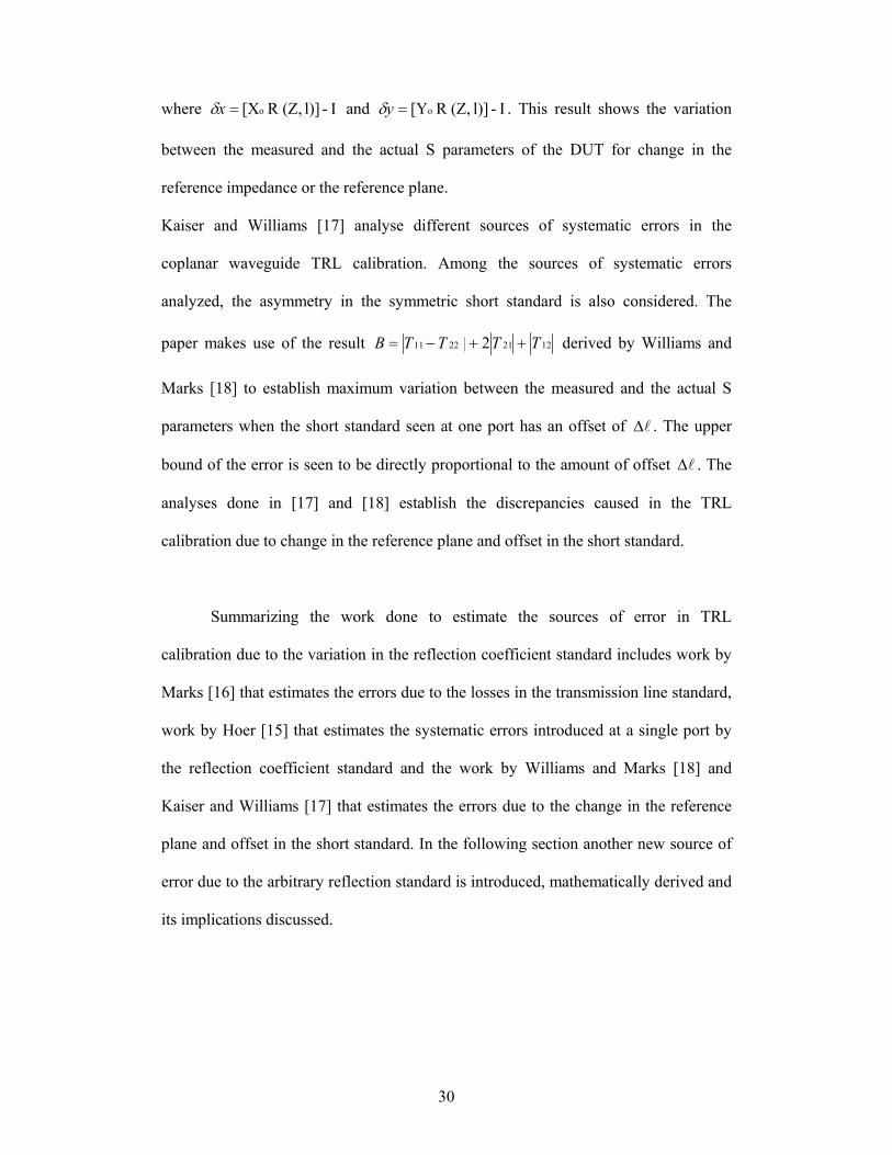
Kaiser and Williams [17] analyse different sources of systematic errors in the
coplanar waveguide TRL calibration. Among the sources of systematic errors
analyzed, the asymmetry in the symmetric short standard is also considered. The
paper makes use of the result 12212211 2 TTTTB ++−= derived by Williams and
Marks [18] to establish maximum variation between the measured and the actual S
parameters when the short standard seen at one port has an offset of l∆ . The upper
bound of the error is seen to be directly proportional to the amount of offset l∆ . The
analyses done in [17] and [18] establish the discrepancies caused in the TRL
calibration due to change in the reference plane and offset in the short standard.
Summarizing the work done to estimate the sources of error in TRL
calibration due to the variation in the reflection coefficient standard includes work by
Marks [16] that estimates the errors due to the losses in the transmission line standard,
work by Hoer [15] that estimates the systematic errors introduced at a single port by
the reflection coefficient standard and the work by Williams and Marks [18] and
Kaiser and Williams [17] that estimates the errors due to the change in the reference
plane and offset in the short standard. In the following section another new source of
error due to the arbitrary reflection standard is introduced, mathematically derived and
its implications discussed.
31
4.1.1 Analysis of the proposed inherent Error in TRL Calibration
This section introduces the proposed errors introduced in the TRL measurements due
to the arbitrary reflection standard. With reference to [1], the TRL calibration does not
assume symmetric and identical fixtures and hence has different error matrices for
both the fixtures that increases the number of standards needed to find the parameters
of the error matrices. The TRL calibration de-embedding procedure by Engen and
Hoer [1] makes use of three standards, the through, an arbitrary reflection standard
whose value need not be known, and a length of transmission line to de-embed the
parameters of the error boxes. The through and the line standards yield two set of
equations that are solved to find the propagation constant and two parameters of one
of the error matrix. In the next step, the two set of measurements obtained by
connecting the unknown reflection standard at the two ports are solved
simultaneously to eliminate the unknown reflection standard and hence making the
TRL de-embedding procedure independent of the unknown reflection standard value.
In the TRL de-embedding procedure an important assumption has been
inherently made, namely that the reflection standard seen at the two ports is exactly
same. This assumption cannot be overlooked as based on this assumption the two sets
of measurements, obtained by connecting the unknown reflection standard at the two
ports, are simultaneously solved to eliminate the unknown reflection standard. Hence
for the TRL de-embedding procedure to be accurate, the unknown reflection standard
seen at the two ports have to be exactly same.
In the following sections analysis is done to see the implications on the
obtained parameters of the error matrices if the reflection standard seen at the two
ports is not exactly same. Let us assume that the arbitrary reflection standard used in
the TRL calibration procedure suffers from repeatability errors and the unknown
32
reflection standard seen at the two ports are not exactly the same value. Let the
reflection standard seen at one port be lΓ and the reflection standard value seen at the
other port be ( ε+Γl ). From the TRL de-embedding procedure mentioned in the
derivation in chapter 3 and in Appendix A, the modified TRL de-embedding
procedure is presented below.
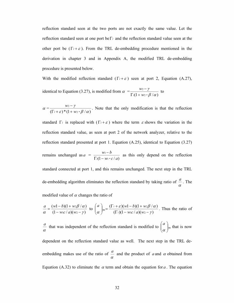
With the modified reflection standard ( ε+Γl ) seen at port 2, Equation (A.27),
identical to Equation (3.27), is modified from α =)/1( *2
2
αβγ
ww
l +Γ− to
α =)/1(*)( *2
2
αβεγw
wl ++Γ
− . Note that the only modification is that the reflection
standard lΓ is replaced with ( ε+Γl ) where the term ε shows the variation in the
reflection standard value, as seen at port 2 of the network analyzer, relative to the
reflection standard presented at port 1. Equation (A.25), identical to Equation (3.27)
remains unchanged asa = )/1( *1
1
acwbw
l −Γ− as this only depend on the reflection
standard connected at port 1, and this remains unchanged. The next step in the TRL
de-embedding algorithm eliminates the reflection standard by taking ratio of αa . The
modified value of α changes the ratio of
))(/1()/1)(1(
21
2
γαβ
α −−+−
=wacwwbwa to
αa
m ))(/1)(()/1)(1)((
21
2
γαβε
−−Γ+−+Γ
=wacwwbw
l
l . Thus the ratio of
αa that was independent of the reflection standard is modified to
αa
m that is now
dependent on the reflection standard value as well. The next step in the TRL de-
embedding makes use of the ratio of αa and the product of a and α obtained from
Equation (A.32) to eliminate the α term and obtain the equation for a . The equation
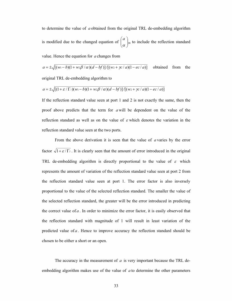
33
to determine the value of a obtained from the original TRL de-embedding algorithm
is modified due to the changed equation of
αa
m to include the reflection standard
value. Hence the equation for a changes from
)]/1)(//[()])(/1)([( 221 aecacwbfdwbwa −+−+−±= γαβ obtained from the
original TRL de-embedding algorithm to
)]/1)(//[()])(/1)()(/1[( 221 aecacwbfdwbwa −+−+−Γ+±= γαβε l
If the reflection standard value seen at port 1 and 2 is not exactly the same, then the
proof above predicts that the term for awill be dependent on the value of the
reflection standard as well as on the value of ε which denotes the variation in the
reflection standard value seen at the two ports.
From the above derivation it is seen that the value of a varies by the error
factor lΓ+ /1 ε . It is clearly seen that the amount of error introduced in the original
TRL de-embedding algorithm is directly proportional to the value of ε which
represents the amount of variation of the reflection standard value seen at port 2 from
the reflection standard value seen at port 1. The error factor is also inversely
proportional to the value of the selected reflection standard. The smaller the value of
the selected reflection standard, the greater will be the error introduced in predicting
the correct value of a . In order to minimize the error factor, it is easily observed that
the reflection standard with magnitude of 1 will result in least variation of the
predicted value ofa . Hence to improve accuracy the reflection standard should be
chosen to be either a short or an open.
The accuracy in the measurement of a is very important because the TRL de-
embedding algorithm makes use of the value of a to determine the other parameters
34
of the fixture error matrices. Any discrepancies will lead to an inaccurate prediction of
the fixture error matrices that will subsequently lead to an inaccurate calculation of
the S parameters of the device under test. In the next paragraph analysis is done to
show how the error factor of lΓ+ /1 ε introduced in the value of a affects the values
of the other fixture error matrix parameters.
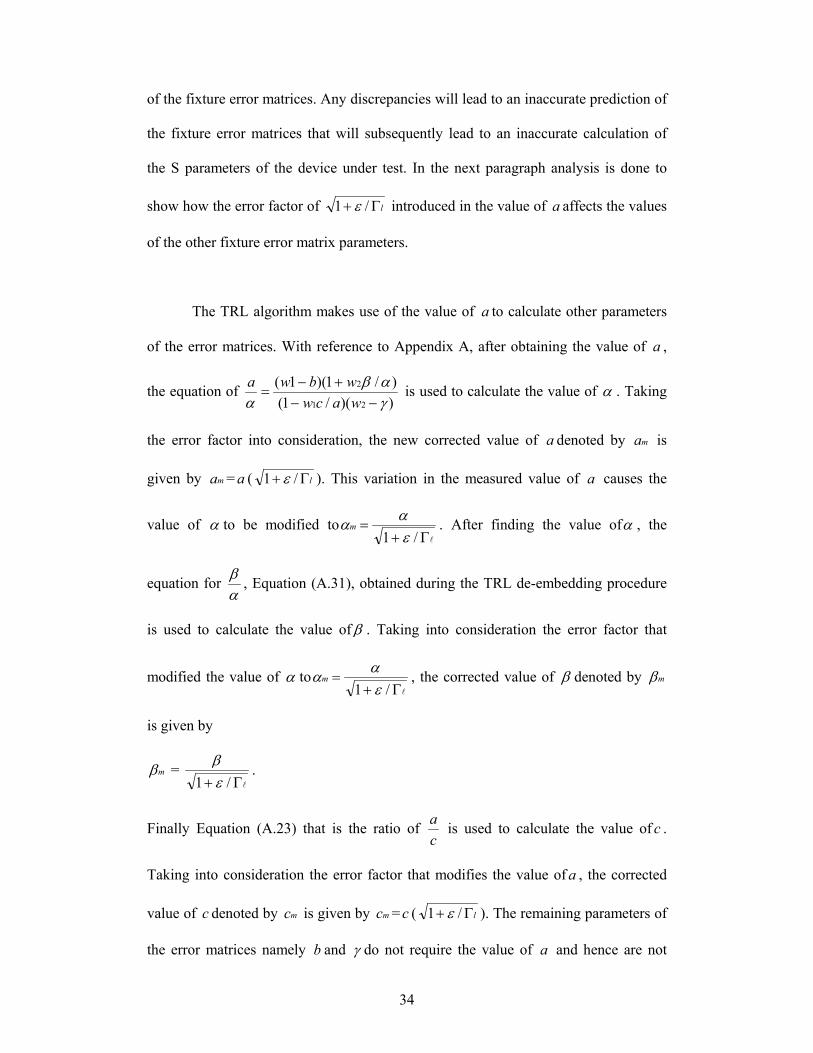
The TRL algorithm makes use of the value of a to calculate other parameters
of the error matrices. With reference to Appendix A, after obtaining the value of a ,
the equation of ))(/1()/1)(1(
21
2
γαβ
α −−+−
=wacwwbwa is used to calculate the value of α . Taking
the error factor into consideration, the new corrected value of a denoted by ma is
given by ma =a ( lΓ+ /1 ε ). This variation in the measured value of a causes the
value of α to be modified tolΓ+
=/1 ε
ααm . After finding the value ofα , the
equation for αβ , Equation (A.31), obtained during the TRL de-embedding procedure
is used to calculate the value ofβ . Taking into consideration the error factor that
modified the value of α tolΓ+
=/1 ε
ααm , the corrected value of β denoted by mβ
is given by
mβ = lΓ+ /1 ε
β .
Finally Equation (A.23) that is the ratio of ca is used to calculate the value of c .
Taking into consideration the error factor that modifies the value ofa , the corrected
value of c denoted by mc is given by mc =c ( lΓ+ /1 ε ). The remaining parameters of
the error matrices namely b and γ do not require the value of a and hence are not
35
affected by the error factor that modifies the value ofa . The analysis presented here
shows how an incorrect prediction of the error parameter a can lead to further
inaccuracies in determining other parameters of the error matrices and ultimately
leading to inaccuracies in determining the S parameters of the device under test.
In the above sections a new source of possible error in the TRL calibration
procedure is introduced and studied in detail. The following sections present an
explanation that delve into the reason for the absence of the errors introduced due to
arbitrary reflection coefficient in a new calibration technique, the Through Line (TL)
calibration that under certain conditions is a replacement to the TRL calibration
procedure. Another phenomenon, the discrepancies in the measurements when the
difference between the through and the line standard approaches integer multiple of a
quarter wavelength, observed in the TRL calibration as well as in the TL calibration
technique is investigated.
4.2 Comparisons between TRL and TL Calibrations
The Through Line (TL) calibration is a two tier calibration procedure. The first step in
TL calibration is to do OSL calibration followed by two set of measurements using
the through and the line standards. The TL calibration, as compared to the TRL
calibration procedure, needs a reduced number of standards for measurements and
requires fewer connections to the microstrip ports improving the repeatability of this
connection. The most important difference between the TRL and the TL calibration is
that in TL calibration the reflection coefficients are derived mathematically (as shown
in chapter 2), which makes it possible to "insert" ideal open and short circuits within a
non-insertable medium such as a dielectric loaded waveguide. Since the value of the
36
reflection standard is mathematically derived, its value is determined accurately as
compared to the TRL calibration procedure where it is seen that a slight variation in
the reflection standard seen at the two ports causes inaccuracies in the measurements.
Another inherent assumption in the TL calibration is that the fixtures are assumed to
be symmetric, as compared to the TRL calibration where the fixtures are assumed to
be non symmetric. As was seen in Chapter 2, symmetric fixturing simplifies the signal
flow graph and makes de-embedding possible with only two set of measurements. In
contrast TRL calibration requires three set of standards. The use of only two standards
in TL calibration as compared to the three standards used in TRL calibration also
reduces discrepancies caused in measurements due to repeatability and connectivity
errors. The TL procedure determines the frequency dependent characteristic
impedance of the line standard. The characteristic impedance of the line standard is
determined from the scattering parameter measurements and the measured free space
capacitance of the reference line.
One inherent drawback present in both the TRL and TL calibration procedure
is the discrepancies in the measurements when the line difference between the through
and the line standard approaches a quarter of a wavelength. The following section
presents analysis that accounts for this cause of discrepancies present in the TRL and
TL calibration technique. Mondal and Chen [2] have presented mathematical analyses
that discuss the cause of discrepancies in the TRL calibration procedure. In the
following section an alternative mathematical analysis is presented to explain why
these discrepancies are likely to be present in any calibration procedure that employs
delay and through as the two standards for calibration.
From the TRL calibration procedure the propagation constant is determined to
be
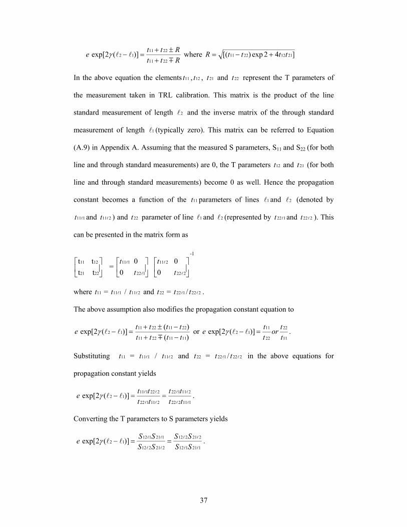
37
eRttRtt
mll
2211
221112 )](2exp[
+±+
=−γ where ]42exp)[( 21122211 ttttR +−=
In the above equation the elements 11t , 12t , 21t and 22t represent the T parameters of
the measurement taken in TRL calibration. This matrix is the product of the line
standard measurement of length 2l and the inverse matrix of the through standard
measurement of length 1l (typically zero). This matrix can be referred to Equation
(A.9) in Appendix A. Assuming that the measured S parameters, S11 and S22 (for both
line and through standard measurements) are 0, the T parameters 12t and 21t (for both
line and through standard measurements) become 0 as well. Hence the propagation
constant becomes a function of the 11t parameters of lines 1l and 2l (denoted by
111lt and 211lt ) and 22t parameter of line 1l and 2l (represented by 122lt and 222lt ). This
can be presented in the matrix form as
-1
22 21
1211
tt tt
=
0
111lt
122
0lt
0
211lt
222
0lt
where 11t = 111lt / 211lt and 22t = 122lt / 222lt .
The above assumption also modifies the propagation constant equation to
e)()()](2exp[
11112211
2211221112
tttttttt
−+−±+
=−m
llγ or e11
22
22
1112 )](2exp[
ttor
tt
=− llγ .
Substituting 11t = 111lt / 211lt and 22t = 122lt / 222lt in the above equations for
propagation constant yields
e111222
211122
211122
22211112 )](2exp[
ll
ll
ll
llll
tttt
tttt
==−γ .
Converting the T parameters to S parameters yields
e121112
221212
221212
12111212 )](2exp[
ll
ll
ll
llll
SSSS
SSSS
==−γ .

38
The following assumption is made that 12S = 21S . With this assumption the above
equations further simplify to e112
212
212
11212 )](exp[
l
l
l
lll
SS
SS
==−γ .
As seen from the above simplified equations, the propagation constant is directly
proportional to the 12S measurements of the line and through standards.
After deriving the equation for the propagation constant, further analysis is
done in the following paragraphs to show the cause of discrepancies in the
measurements when the difference between the delay standards approach an integer
multiple of a half wavelength.
The propagation constant derived for the line standard can be represented in
magnitude and phase notation or as )](exp[* 212112212
112ll
l
lSSje
SS
p ∠−∠= . The
magnitude phase notation can also be represented in complex number notation as
jIRp += where )cos( 212112212
112ll
l
lSS
SS
R ∠−∠= and
)sin( 212112212
112ll
l
lSS
SS
I ∠−∠= .
From the real and imaginary terms of the propagation constant equation, it is seen that
the determination of the propagation constant is dependent on the insertion phase of
the delay standard. The insertion phase of a line is directly proportional to the
frequency and the line length and inversely proportional to the wavelength. Hence the
selection of the line length, which is the difference between the line lengths of the two
delay standards, the through and the line standard in TRL and TL calibration, decides
the insertion phase. When the line difference approaches a quarter of a wavelength,
the insertion phase approaches 90º.
39
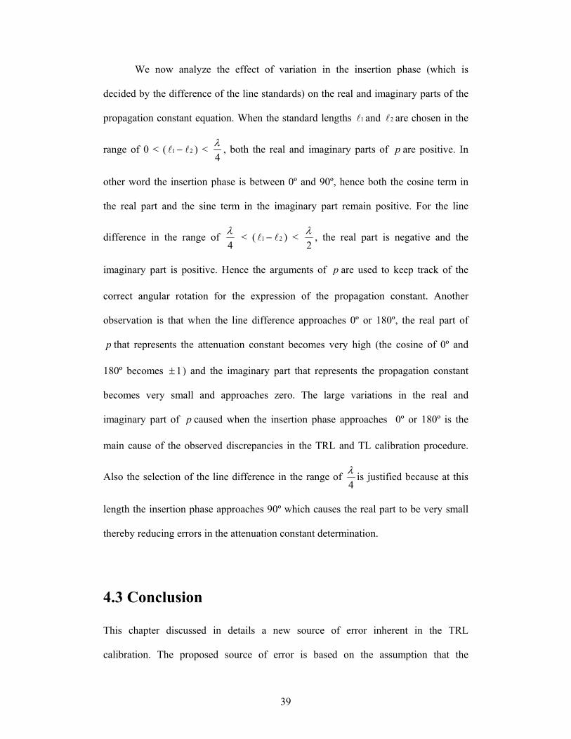
We now analyze the effect of variation in the insertion phase (which is
decided by the difference of the line standards) on the real and imaginary parts of the
propagation constant equation. When the standard lengths 1l and 2l are chosen in the
range of 0 < ( 21 ll − ) < 4λ , both the real and imaginary parts of p are positive. In
other word the insertion phase is between 0º and 90º, hence both the cosine term in
the real part and the sine term in the imaginary part remain positive. For the line
difference in the range of 4λ < ( 21 ll − ) <
2λ , the real part is negative and the
imaginary part is positive. Hence the arguments of p are used to keep track of the
correct angular rotation for the expression of the propagation constant. Another
observation is that when the line difference approaches 0º or 180º, the real part of
p that represents the attenuation constant becomes very high (the cosine of 0º and
180º becomes 1± ) and the imaginary part that represents the propagation constant
becomes very small and approaches zero. The large variations in the real and
imaginary part of p caused when the insertion phase approaches 0º or 180º is the
main cause of the observed discrepancies in the TRL and TL calibration procedure.
Also the selection of the line difference in the range of 4λ is justified because at this
length the insertion phase approaches 90º which causes the real part to be very small
thereby reducing errors in the attenuation constant determination.
4.3 Conclusion
This chapter discussed in details a new source of error inherent in the TRL
calibration. The proposed source of error is based on the assumption that the
40
reflection standard value seen at the two ports of the network analyzer are not exactly
same. The TRL calibration method is compared with the new calibration method, the
TL calibration to explain why this calibration, under certain conditions is a better
alternative to TRL calibration. The proposed source of error present in TRL
calibration is avoided in TL calibration because it makes use of symmetry fixtures and
synthesized reflection co-efficient that simplifies the error model and reduces the
number of standards needed thereby reducing the repeatability error. Another
drawback of TRL namely the accurate determination of the characteristic impedance
is removed in TL calibration by determining the impedance of the line from the
scattering parameters measurements and the measured free space capacitance of the
line. Finally the cause of discrepancies in the TRL and TL calibration measurement
when the difference in the length of the through and line standard approaches 0 or
2λ is discussed.
41
Chapter 5: Experimental Results The proposed discrepancies introduced in the parameters of the error boxes A and B
due to the arbitrary reflection coefficient are verified experimentally. The proposed
error model is based on the assumption that the reflection standard value seen at the
two ports are not exactly same. In the experimental setup, this assumption is verified
experimentally. Experimental analysis is done using symmetric fixture on the device
under test and the readings are processed with the TRL algorithm implemented in
MATLAB to obtain the parameters of the error box A and B. Next the error factor
term introduced due to mismatch in the reflection coefficient is introduced into the
MATLAB implementation of the TRL algorithm and the new set of parameters for
the error box A and B are obtained. The above process is repeated for different
reflection coefficient standards to obtain an optimal value of reflection standard that
result in least error. The results are verified and presented in this chapter.
5.1 General Measurement Steps
The network analyzer measurement system consists of the source, the test set, the
vector signal processor and the display. These together comprise the stimulus and
response test system that measures the signal transmitted through the device and the
reflected signal from the input of the device. The data is then processed to display the
magnitude and phase responses. For our measurements a Hewlett Packard 8510
network analyzer system is used. This network analyzer contains a sweeper to provide
the RF stimulus. The test set provides the points where the device under test is to be
connected. The system uses coaxial test sets up to frequency range of 50 GHz. The
front panel of network analyzer includes the CRT that displays the measurement
42
results. The network analyzer has two channels for displaying the measurements at
the two test ports. ‘Channel 1’ or ‘Channel 2’ selects the channel display. The keys in
the ‘Stimulus’, ‘Parameter’, ‘Format’ and ‘Response’ blocks are needed for the
measurement setup, calibration, data representation and data output functions.
Following are the general measurement sequence involved while taking
measurements. The first step is to setup the test port cables and select suitable
connectors for the device under test. The next step is to setup the network analyzer,
which involves using the keys in the ‘Stimulus’ block to set the desired start and stop
frequencies, number of measured points and characteristic of frequency sweep. The
keys in the ‘Parameter’ block decide the parameters to be measured and displayed.
The keys in the ‘Format’ and ‘Response’ blocks are used for selecting type of display
and position of the trace to view the measured data respectively. Next step is to select
the appropriate calibration standard to correct the systematic errors using the keys in
the ‘Cal’ block. Once the measurements have been taken, the ‘save’ key stores the
measured data in internal/external storage. The ‘Marker’ key and knob is used to
position the measurement markers to the points of interest on the trace and store these
results without further recalibration. The above-mentioned steps give a brief outline to
take basic measurements in network analyzer and introduce the reader to the network
analyzer control keys.
5.2 Experiment Setup
After an overview of the basic control keys and measurement sequence, we discuss in
detail the fixtures used for our measurement setup, the components used and the
procedure employed in getting the corrected measured S parameters of the device
under test.
43
Before starting with the measurements the network analyzer need to be
configured by the user to display the measurements accordingly. The front panel keys
mentioned in the above section can easily configure the network analyzer. The
following steps mentioned here provide an overview of the configuration settings
used by us in taking the measurements. The keys in the ‘Stimulus’ block are used to
set the frequency sweep, the sweep time and the number of frequency points to be
measured to 801 points. The ‘start’ and ‘stop’ keys and the ‘center’ and ‘span’ keys
on the ‘Stimulus’ block are used to set the limits of the frequency sweep. Pressing the
‘Stimulus’ menu key gives options to set the sweep time, number of points and sweep
modes. To select the number of points, press the ‘Number of points’ softkey to select
the 801 points. The ‘Ramp’, ‘Step’ and ‘Frequency List’ softkeys select the sweep
mode. The keys in the ‘Parameter’ block allow the user to select the S parameters to
be measured. In our experiment all the S parameters were measured and stored. The
next step after configuring the network analyzer for measurements is to perform the
measurement calibration. The keys on the ‘Format’ block provide a comprehensive
selection of keys to display the measurements in different display formats. The
calibration kit used is a Hewlett Packard 85050 7 millimeters Calibration Kit. The
calibration standard definitions for the above mentioned Calibration Kit are stored in
the internal memory of the network analyzer prior to starting the measurements. The
standard definitions provide the constants needed to mathematically model the
electrical characteristics of the standards used in the Calibration Kit.
The point where the device under test is connected is called the ‘Reference
Plane’, which is the end of the coaxial cable. In our case the test set consists of the
coaxial cables and fixtures that connect the network analyzer and the coaxial cable.
44
Calibration is necessary before taking measurements as the interconnecting of the test
set coaxial cables influences the accuracy of the measurement. In order to remove
these systematic errors the Open-Short-Load (OSL) calibration method is used to
setup the reference plane to the coaxial probe tips at port 1 and 2 of the network
analyzer. For better accuracy low band load is used as the ‘Load’ standard in OSL
calibration for frequencies below 2 GHz and the sliding load is used for measurement
above 2 GHz. Since the frequency range for our measurement is up to 18 GHz, sliding
load standard is used in the OSL calibration. The main aim of the experiment is to
obtain the parameters of the error box A and B and finally obtain the correct S
parameters of the device under test by implementing the TRL algorithms and the
modified TRL algorithm that takes into consideration the error factor introduced due
to arbitrary reflection standard and compare their differences. In order to introduce
these errors, symmetrical fixtures are introduced in between the reference plane and
the device under test. The symmetrical fixtures are constructed from connecting
“7mm - SMA type adapter to 90º bend SAM type to SMA – 7mm type adapter” at
both ends of the test set coaxial cables. The next step after the OSL calibration is to
select the Calibration kit. In our experimental setup, for maximum accuracy, the
FULL 2-PORT calibration choice offered in the network analyzer HP 8510 is
selected. The FULL 2-PORT calibration uses Open, Short and Load standards at each
port 1 and 2 of the network analyzer. The FULL 2-PORT calibration is selected in the
network analyzer from the Cal type selection menu. In the following paragraph, the
different steps involved in the FULL 2-PORT calibration method implemented in our
experimental setup are listed.
The first three steps involve connecting the short, open and load standards at
the two ends of the connected fixtures and noting the reflection coefficient value,
45
yielding six sets of measurements. The next four steps involve connecting a 20 dB
attenuator and open/short standards at the two reference planes, which are the ends of
the connected fixtures. Similar measurements are taken by replacing the 20 dB
attenuator with a 50 dB attenuator. In the next step, the 20 dB attenuator is connected
between the two fixture ends. For the thru measurement, the two fixture ends are
connected together. The next step involves connecting the 20 dB attenuator and a 10
cm air line between the reference planes, which are the two ends of the connected
fixtures. Similar measurements are taken by replacing the 20 dB attenuator with a 50
dB attenuator. The calibration kit used for our set of measurements did not contain the
‘Reflect’ standard. In other words, the TRL calibration kit is not unavailable. Hence
the TRL deembedding algorithm is implemented in MATLAB and the set of
measurements obtained from the FULL 2-PORT CALBRATION are fed into the
MATLAB code that processes the set of measurements, performs the TRL
deembedding algorithm and displays the results. The following section presents the
observed results for the above set of measurements taken and confirms the theoretical
assumption of discrepancies in the observed reflection coefficient seen at the two ends
of the reference planes, which are the two ends of the connected symmetrical fixtures.
46
5.3 MATLAB Simulation Results In the following paragraphs, the measurements obtained from the experimental
procedure, as mentioned in the previous section, are presented. The measured data
obtained from the above mentioned steps are fed into the MATLAB code that
implements the TRL deembedding algorithm. After processing the data, the reflection
coefficients seen at the ports of the network analyzer are seen to be different. The
proposed source of discrepancies in TRL calibration was based on the following
assumption that the reflection coefficients seen at the end of the two ports of the
network analyzer are different. This assumption is verified by the MATLAB code.
The MATLAB code further implements the modified TRL deembedding procedure
that estimates the amount of error introduced in the error boxes A and B due to the
observed discrepancies in the reflection coefficient seen at the end of the ports of the
network analyzer.
5.3.1 TRL calibration results obtained from using short and open
standards
The experimental analysis is done is by implementing TRL algorithm on three
different devices under test and then comparing their results. The first device under
test is an air filled transmission line connected between the ends of the two fixtures.
The second device under test used is a 20dB attenuator. The third device used is a
combination of 20dB attenuator and an air filled transmission line.
Figure 5.1 shown in the next page shows the data obtained from the network
analyzer in magnitude and phase response for the reflection coefficient of the short
standard connected at the two symmetrical fixture ends.
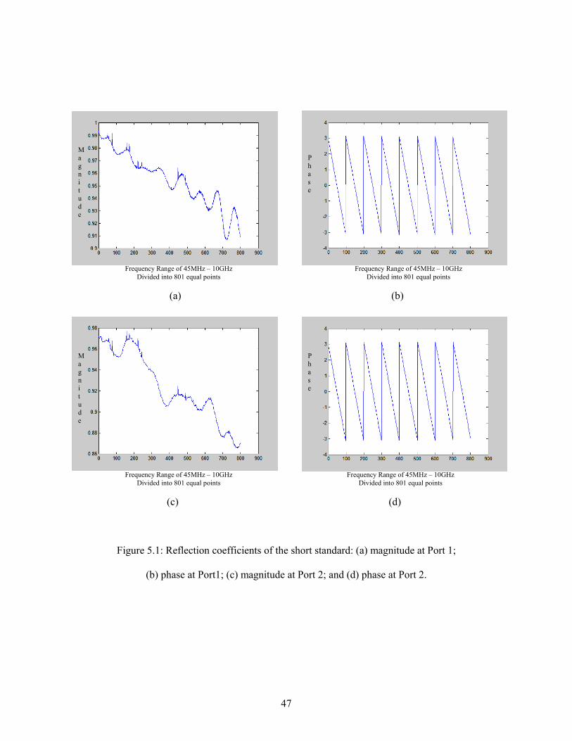
47
(a) (b)
(c) (d)
Figure 5.1: Reflection coefficients of the short standard: (a) magnitude at Port 1;
(b) phase at Port1; (c) magnitude at Port 2; and (d) phase at Port 2.
M a g n i t u d e
M a g n i t u d e
P h a s e
Frequency Range of 45MHz – 10GHz Divided into 801 equal points
Frequency Range of 45MHz – 10GHz Divided into 801 equal points
Frequency Range of 45MHz – 10GHz Divided into 801 equal points
Frequency Range of 45MHz – 10GHz Divided into 801 equal points
P h a s e
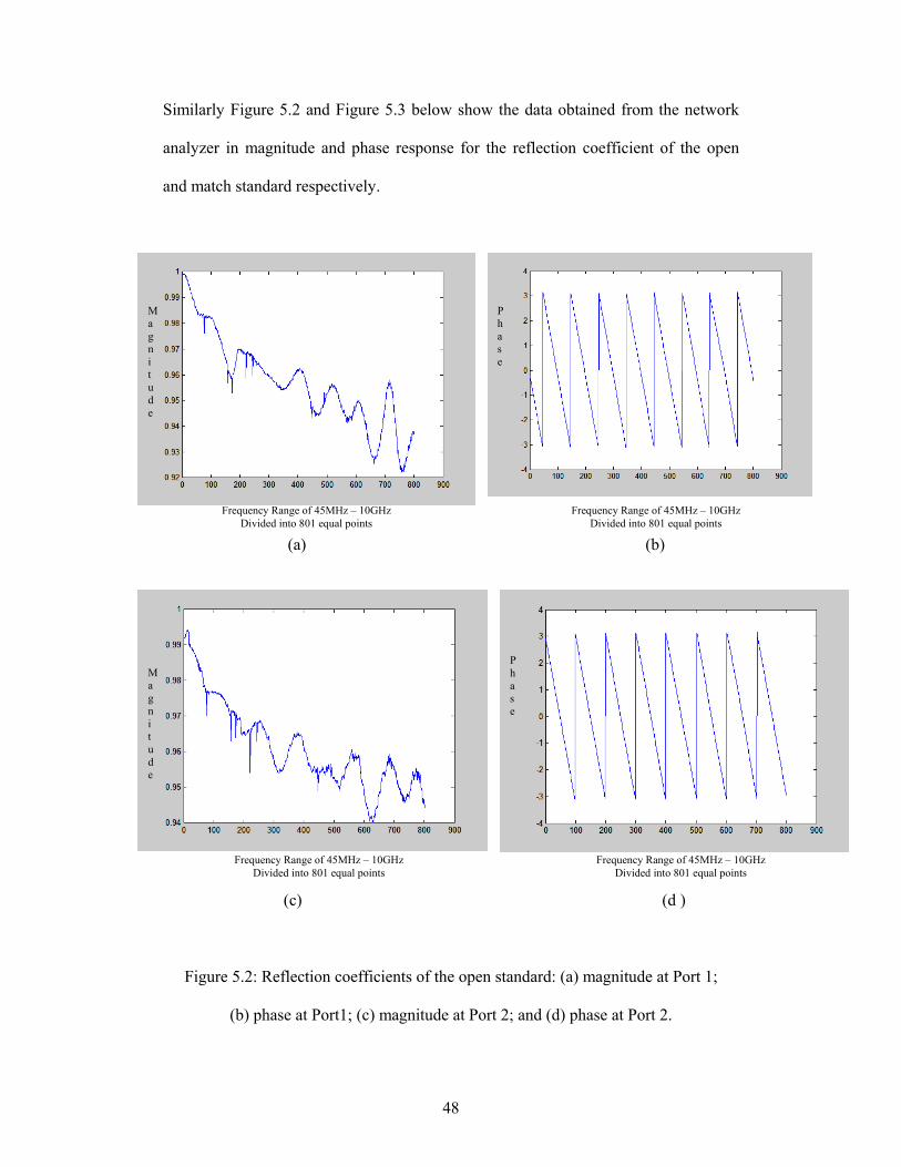
48
Similarly Figure 5.2 and Figure 5.3 below show the data obtained from the network
analyzer in magnitude and phase response for the reflection coefficient of the open
and match standard respectively.
(a) (b)
(c) (d )
Figure 5.2: Reflection coefficients of the open standard: (a) magnitude at Port 1;
(b) phase at Port1; (c) magnitude at Port 2; and (d) phase at Port 2.
Frequency Range of 45MHz – 10GHz Divided into 801 equal points
Frequency Range of 45MHz – 10GHz Divided into 801 equal points
Frequency Range of 45MHz – 10GHz Divided into 801 equal points
Frequency Range of 45MHz – 10GHz Divided into 801 equal points
M a g n i t u d e
M a g n i t u d e
P h a s e
P h a s e
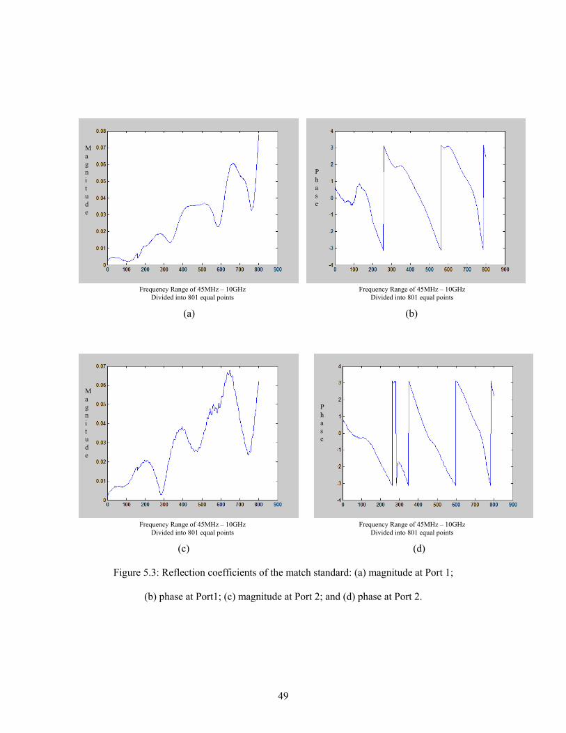
49
(a) (b)
(c) (d)
Figure 5.3: Reflection coefficients of the match standard: (a) magnitude at Port 1;
(b) phase at Port1; (c) magnitude at Port 2; and (d) phase at Port 2.
Frequency Range of 45MHz – 10GHz Divided into 801 equal points
Frequency Range of 45MHz – 10GHz Divided into 801 equal points
Frequency Range of 45MHz – 10GHz Divided into 801 equal points
Frequency Range of 45MHz – 10GHz Divided into 801 equal points
M a g n i t u d e
M a g n i t u d e
P h a s e
P h a s e
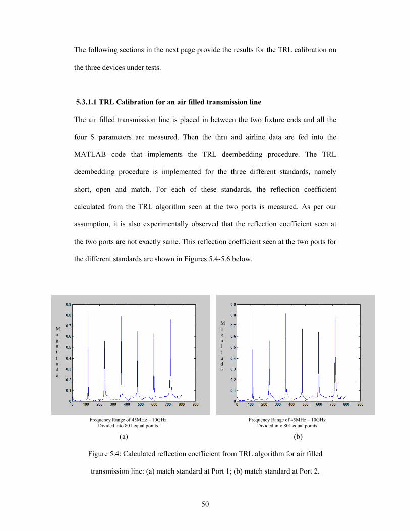
50
The following sections in the next page provide the results for the TRL calibration on
the three devices under tests.
5.3.1.1 TRL Calibration for an air filled transmission line
The air filled transmission line is placed in between the two fixture ends and all the
four S parameters are measured. Then the thru and airline data are fed into the
MATLAB code that implements the TRL deembedding procedure. The TRL
deembedding procedure is implemented for the three different standards, namely
short, open and match. For each of these standards, the reflection coefficient
calculated from the TRL algorithm seen at the two ports is measured. As per our
assumption, it is also experimentally observed that the reflection coefficient seen at
the two ports are not exactly same. This reflection coefficient seen at the two ports for
the different standards are shown in Figures 5.4-5.6 below.
(a) (b)
Figure 5.4: Calculated reflection coefficient from TRL algorithm for air filled
transmission line: (a) match standard at Port 1; (b) match standard at Port 2.
Frequency Range of 45MHz – 10GHz Divided into 801 equal points
Frequency Range of 45MHz – 10GHz Divided into 801 equal points
M a g n i t u d e
M a g n i t u d e
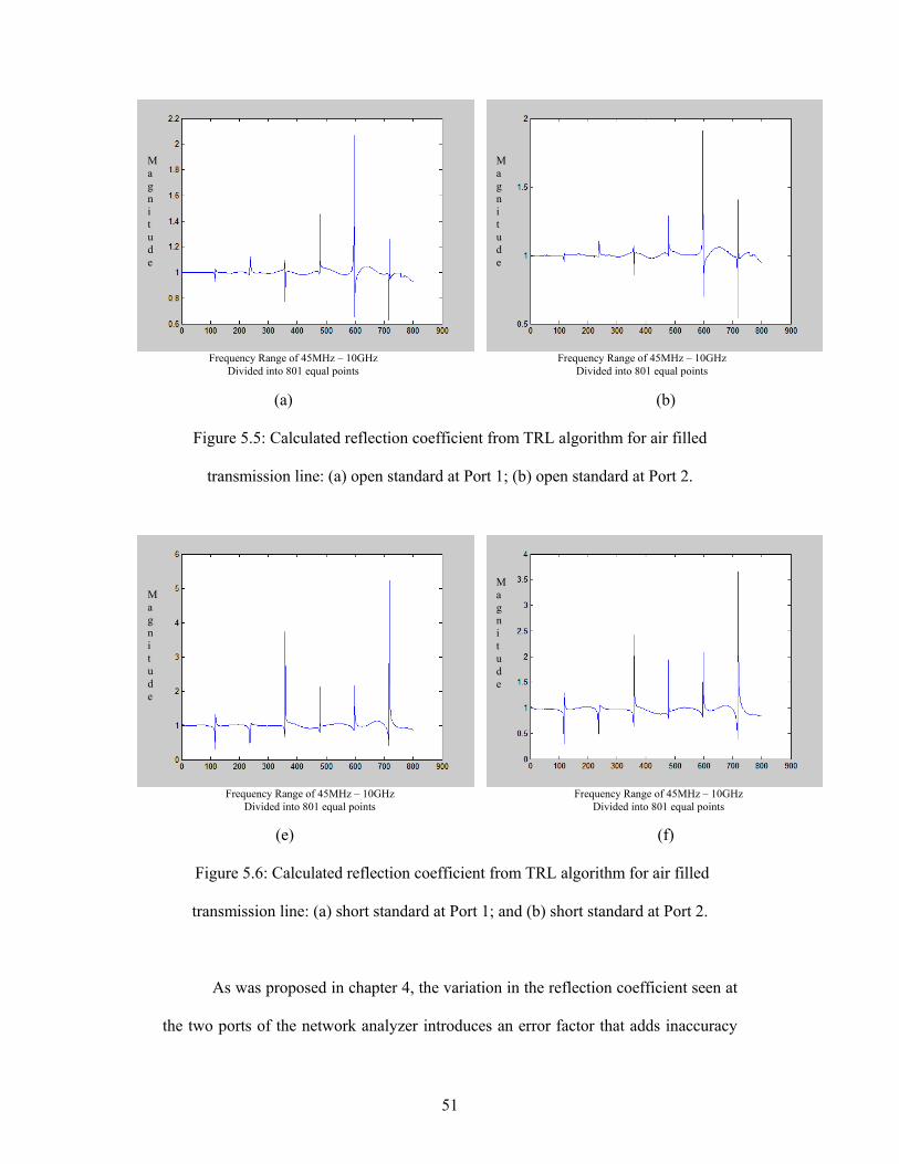
51
(a) (b)
Figure 5.5: Calculated reflection coefficient from TRL algorithm for air filled
transmission line: (a) open standard at Port 1; (b) open standard at Port 2.
(e) (f)
Figure 5.6: Calculated reflection coefficient from TRL algorithm for air filled
transmission line: (a) short standard at Port 1; and (b) short standard at Port 2.
As was proposed in chapter 4, the variation in the reflection coefficient seen at
the two ports of the network analyzer introduces an error factor that adds inaccuracy
Frequency Range of 45MHz – 10GHz Divided into 801 equal points
Frequency Range of 45MHz – 10GHz Divided into 801 equal points
Frequency Range of 45MHz – 10GHz Divided into 801 equal points
Frequency Range of 45MHz – 10GHz Divided into 801 equal points
M a g n i t u d e
M a g n i t u d e
M a g n i t u d e
M a g n i t u d e
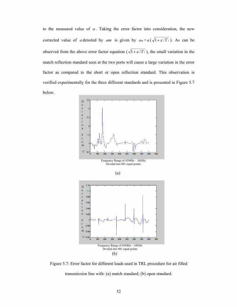
52
to the measured value of a . Taking the error factor into consideration, the new
corrected value of a denoted by am is given by ma = a ( lΓ+ /1 ε ). As can be
observed from the above error factor equation ( lΓ+ /1 ε ), the small variation in the
match reflection standard seen at the two ports will cause a large variation in the error
factor as compared to the short or open reflection standard. This observation is
verified experimentally for the three different standards and is presented in Figure 5.7
below.
(a)
(b)
Figure 5.7: Error factor for different loads used in TRL procedure for air filled
transmission line with: (a) match standard; (b) open standard.
D e v i a t i o n F r o m ‘1’
D e v i a t i o n F r o m ‘1’
Frequency Range of 45MHz – 10GHz Divided into 801 equal points
Frequency Range of 45MHz – 10GHz Divided into 801 equal points
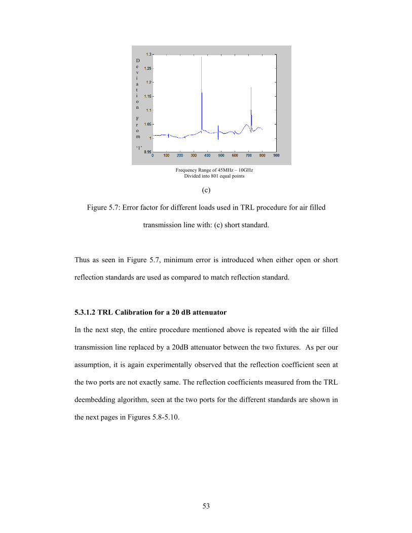
53
(c)
Figure 5.7: Error factor for different loads used in TRL procedure for air filled
transmission line with: (c) short standard.
Thus as seen in Figure 5.7, minimum error is introduced when either open or short
reflection standards are used as compared to match reflection standard.
5.3.1.2 TRL Calibration for a 20 dB attenuator
In the next step, the entire procedure mentioned above is repeated with the air filled
transmission line replaced by a 20dB attenuator between the two fixtures. As per our
assumption, it is again experimentally observed that the reflection coefficient seen at
the two ports are not exactly same. The reflection coefficients measured from the TRL
deembedding algorithm, seen at the two ports for the different standards are shown in
the next pages in Figures 5.8-5.10.
D e v i a t i o n F r o m ‘1’
Frequency Range of 45MHz – 10GHz Divided into 801 equal points
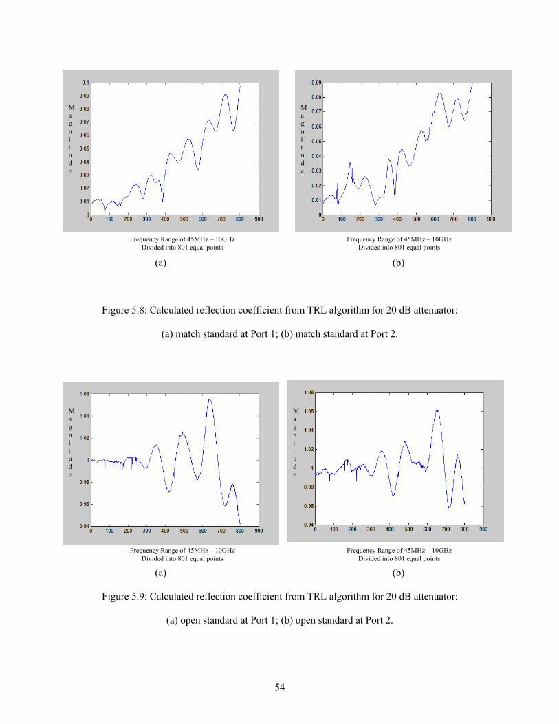
54
(a) (b)
Figure 5.8: Calculated reflection coefficient from TRL algorithm for 20 dB attenuator:
(a) match standard at Port 1; (b) match standard at Port 2.
(a) (b)
Figure 5.9: Calculated reflection coefficient from TRL algorithm for 20 dB attenuator:
(a) open standard at Port 1; (b) open standard at Port 2.
Frequency Range of 45MHz – 10GHz Divided into 801 equal points
Frequency Range of 45MHz – 10GHz Divided into 801 equal points
Frequency Range of 45MHz – 10GHz Divided into 801 equal points
Frequency Range of 45MHz – 10GHz Divided into 801 equal points
M a g n i t u d e
M a g n i t u d e
M a g n i t u d e
M a g n i t u d e
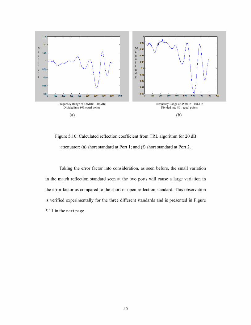
55
(a) (b)
Figure 5.10: Calculated reflection coefficient from TRL algorithm for 20 dB
attenuator: (a) short standard at Port 1; and (f) short standard at Port 2.
Taking the error factor into consideration, as seen before, the small variation
in the match reflection standard seen at the two ports will cause a large variation in
the error factor as compared to the short or open reflection standard. This observation
is verified experimentally for the three different standards and is presented in Figure
5.11 in the next page.
Frequency Range of 45MHz – 10GHz Divided into 801 equal points
Frequency Range of 45MHz – 10GHz Divided into 801 equal points
M a g n i t u d e
M a g n i t u d e
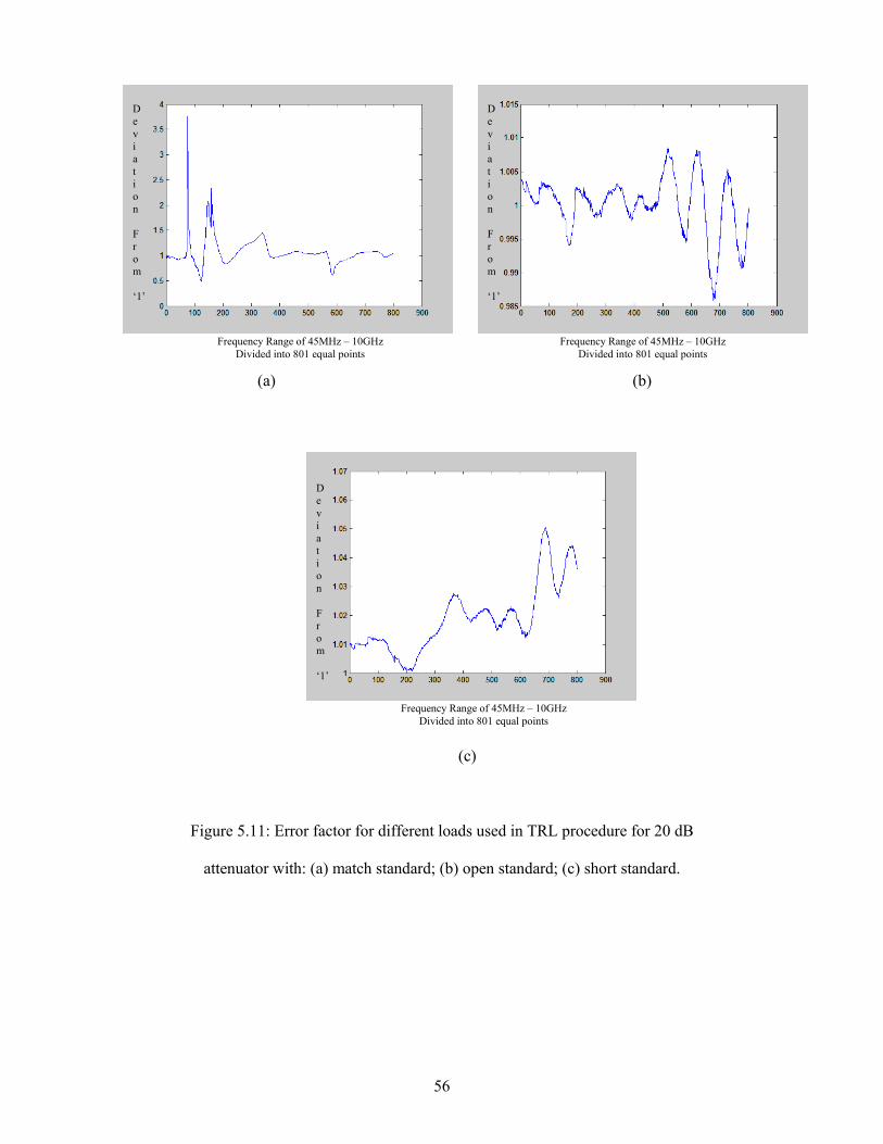
56
(a) (b)
(c)
Figure 5.11: Error factor for different loads used in TRL procedure for 20 dB
attenuator with: (a) match standard; (b) open standard; (c) short standard.
D e v i a t i o n F r o m ‘1’
D e v i a t i o n F r o m ‘1’
D e v i a t i o n F r o m ‘1’
Frequency Range of 45MHz – 10GHz Divided into 801 equal points
Frequency Range of 45MHz – 10GHz Divided into 801 equal points
Frequency Range of 45MHz – 10GHz Divided into 801 equal points
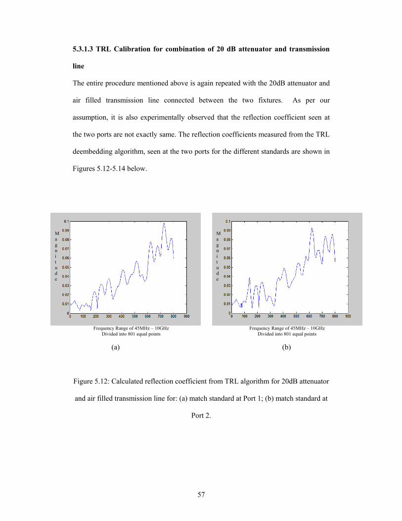
57
5.3.1.3 TRL Calibration for combination of 20 dB attenuator and transmission
line
The entire procedure mentioned above is again repeated with the 20dB attenuator and
air filled transmission line connected between the two fixtures. As per our
assumption, it is also experimentally observed that the reflection coefficient seen at
the two ports are not exactly same. The reflection coefficients measured from the TRL
deembedding algorithm, seen at the two ports for the different standards are shown in
Figures 5.12-5.14 below.
(a) (b)
Figure 5.12: Calculated reflection coefficient from TRL algorithm for 20dB attenuator
and air filled transmission line for: (a) match standard at Port 1; (b) match standard at
Port 2.
Frequency Range of 45MHz – 10GHz Divided into 801 equal points
Frequency Range of 45MHz – 10GHz Divided into 801 equal points
M a g n i t u d e
M a g n i t u d e
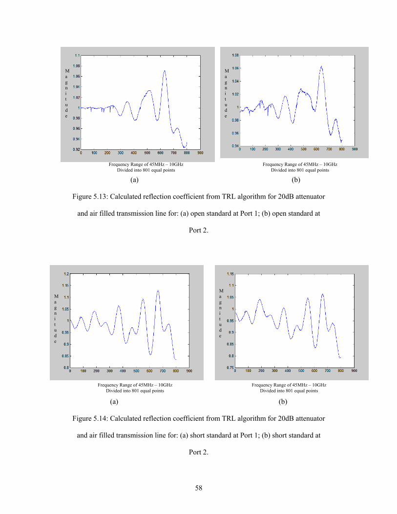
58
(a) (b)
Figure 5.13: Calculated reflection coefficient from TRL algorithm for 20dB attenuator
and air filled transmission line for: (a) open standard at Port 1; (b) open standard at
Port 2.
(a) (b)
Figure 5.14: Calculated reflection coefficient from TRL algorithm for 20dB attenuator
and air filled transmission line for: (a) short standard at Port 1; (b) short standard at
Port 2.
Frequency Range of 45MHz – 10GHz Divided into 801 equal points
Frequency Range of 45MHz – 10GHz Divided into 801 equal points
Frequency Range of 45MHz – 10GHz Divided into 801 equal points
Frequency Range of 45MHz – 10GHz Divided into 801 equal points
M a g n i t u d e
M a g n i t u d e
M a g n i t u d e
M a g n i t u d e
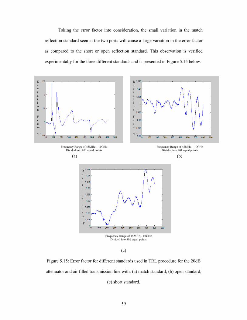
59
Taking the error factor into consideration, the small variation in the match
reflection standard seen at the two ports will cause a large variation in the error factor
as compared to the short or open reflection standard. This observation is verified
experimentally for the three different standards and is presented in Figure 5.15 below.
(a) (b)
(c)
Figure 5.15: Error factor for different standards used in TRL procedure for the 20dB
attenuator and air filled transmission line with: (a) match standard; (b) open standard;
(c) short standard.
D e v i a t i o n F r o m ‘1’
D e v i a t i o n F r o m ‘1’
D e v i a t i o n F r o m ‘1’
Frequency Range of 45MHz – 10GHz Divided into 801 equal points
Frequency Range of 45MHz – 10GHz Divided into 801 equal points
Frequency Range of 45MHz – 10GHz Divided into 801 equal points
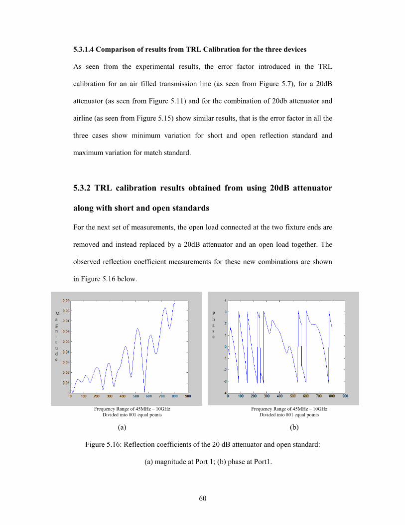
60
5.3.1.4 Comparison of results from TRL Calibration for the three devices
As seen from the experimental results, the error factor introduced in the TRL
calibration for an air filled transmission line (as seen from Figure 5.7), for a 20dB
attenuator (as seen from Figure 5.11) and for the combination of 20db attenuator and
airline (as seen from Figure 5.15) show similar results, that is the error factor in all the
three cases show minimum variation for short and open reflection standard and
maximum variation for match standard.
5.3.2 TRL calibration results obtained from using 20dB attenuator
along with short and open standards
For the next set of measurements, the open load connected at the two fixture ends are
removed and instead replaced by a 20dB attenuator and an open load together. The
observed reflection coefficient measurements for these new combinations are shown
in Figure 5.16 below.
(a) (b)
Figure 5.16: Reflection coefficients of the 20 dB attenuator and open standard:
(a) magnitude at Port 1; (b) phase at Port1.
Frequency Range of 45MHz – 10GHz Divided into 801 equal points
Frequency Range of 45MHz – 10GHz Divided into 801 equal points
P h a s e
M a g n i t u d e
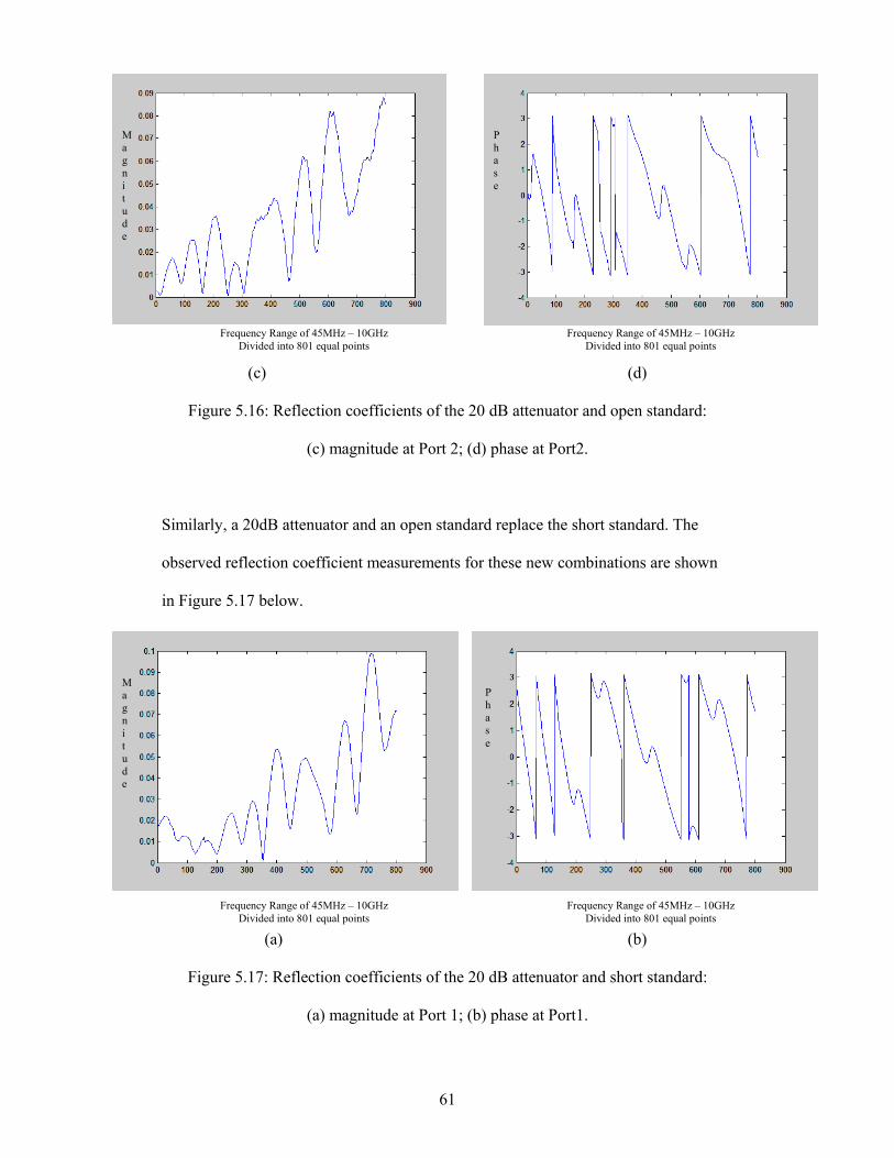
61
(c) (d)
Figure 5.16: Reflection coefficients of the 20 dB attenuator and open standard:
(c) magnitude at Port 2; (d) phase at Port2.
Similarly, a 20dB attenuator and an open standard replace the short standard. The
observed reflection coefficient measurements for these new combinations are shown
in Figure 5.17 below.
(a) (b)
Figure 5.17: Reflection coefficients of the 20 dB attenuator and short standard:
(a) magnitude at Port 1; (b) phase at Port1.
Frequency Range of 45MHz – 10GHz Divided into 801 equal points
Frequency Range of 45MHz – 10GHz Divided into 801 equal points
Frequency Range of 45MHz – 10GHz Divided into 801 equal points
Frequency Range of 45MHz – 10GHz Divided into 801 equal points
M a g n i t u d e
M a g n i t u d e
P h a s e
P h a s e
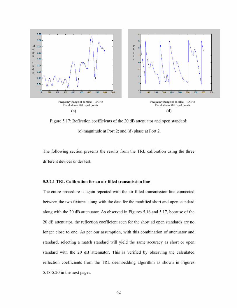
62
(c) (d)
Figure 5.17: Reflection coefficients of the 20 dB attenuator and open standard:
(c) magnitude at Port 2; and (d) phase at Port 2.
The following section presents the results from the TRL calibration using the three
different devices under test.
5.3.2.1 TRL Calibration for an air filled transmission line
The entire procedure is again repeated with the air filled transmission line connected
between the two fixtures along with the data for the modified short and open standard
along with the 20 dB attenuator. As observed in Figures 5.16 and 5.17, because of the
20 dB attenuator, the reflection coefficient seen for the short ad open standards are no
longer close to one. As per our assumption, with this combination of attenuator and
standard, selecting a match standard will yield the same accuracy as short or open
standard with the 20 dB attenuator. This is verified by observing the calculated
reflection coefficients from the TRL deembedding algorithm as shown in Figures
5.18-5.20 in the next pages.
Frequency Range of 45MHz – 10GHz Divided into 801 equal points
Frequency Range of 45MHz – 10GHz Divided into 801 equal points
M a g n i t u d e
P h a s e
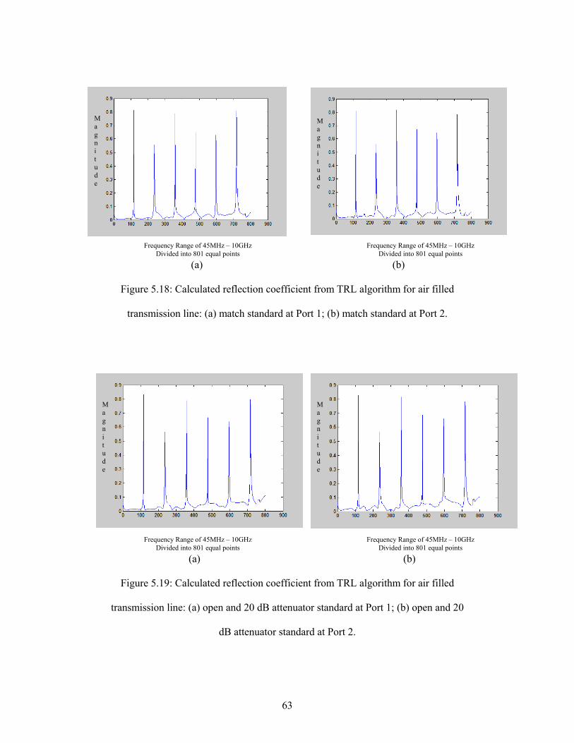
63
(a) (b)
Figure 5.18: Calculated reflection coefficient from TRL algorithm for air filled
transmission line: (a) match standard at Port 1; (b) match standard at Port 2.
(a) (b)
Figure 5.19: Calculated reflection coefficient from TRL algorithm for air filled
transmission line: (a) open and 20 dB attenuator standard at Port 1; (b) open and 20
dB attenuator standard at Port 2.
Frequency Range of 45MHz – 10GHz Divided into 801 equal points
Frequency Range of 45MHz – 10GHz Divided into 801 equal points
Frequency Range of 45MHz – 10GHz Divided into 801 equal points
Frequency Range of 45MHz – 10GHz Divided into 801 equal points
M a g n i t u d e
M a g n i t u d e
M a g n i t u d e
M a g n i t u d e
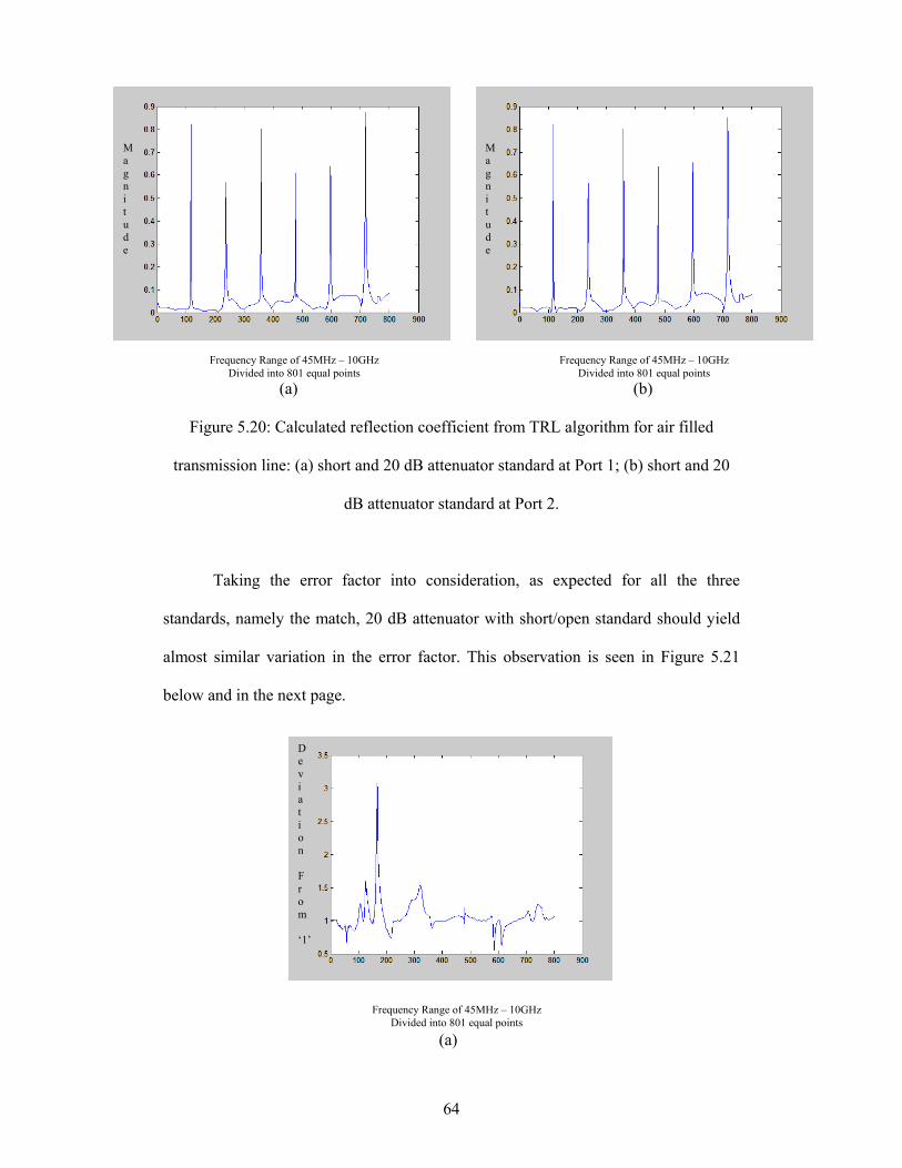
64
(a) (b)
Figure 5.20: Calculated reflection coefficient from TRL algorithm for air filled
transmission line: (a) short and 20 dB attenuator standard at Port 1; (b) short and 20
dB attenuator standard at Port 2.
Taking the error factor into consideration, as expected for all the three
standards, namely the match, 20 dB attenuator with short/open standard should yield
almost similar variation in the error factor. This observation is seen in Figure 5.21
below and in the next page.
(a)
D e v i a t i o n F r o m ‘1’
Frequency Range of 45MHz – 10GHz Divided into 801 equal points
Frequency Range of 45MHz – 10GHz Divided into 801 equal points
Frequency Range of 45MHz – 10GHz Divided into 801 equal points
M a g n i t u d e
M a g n i t u d e
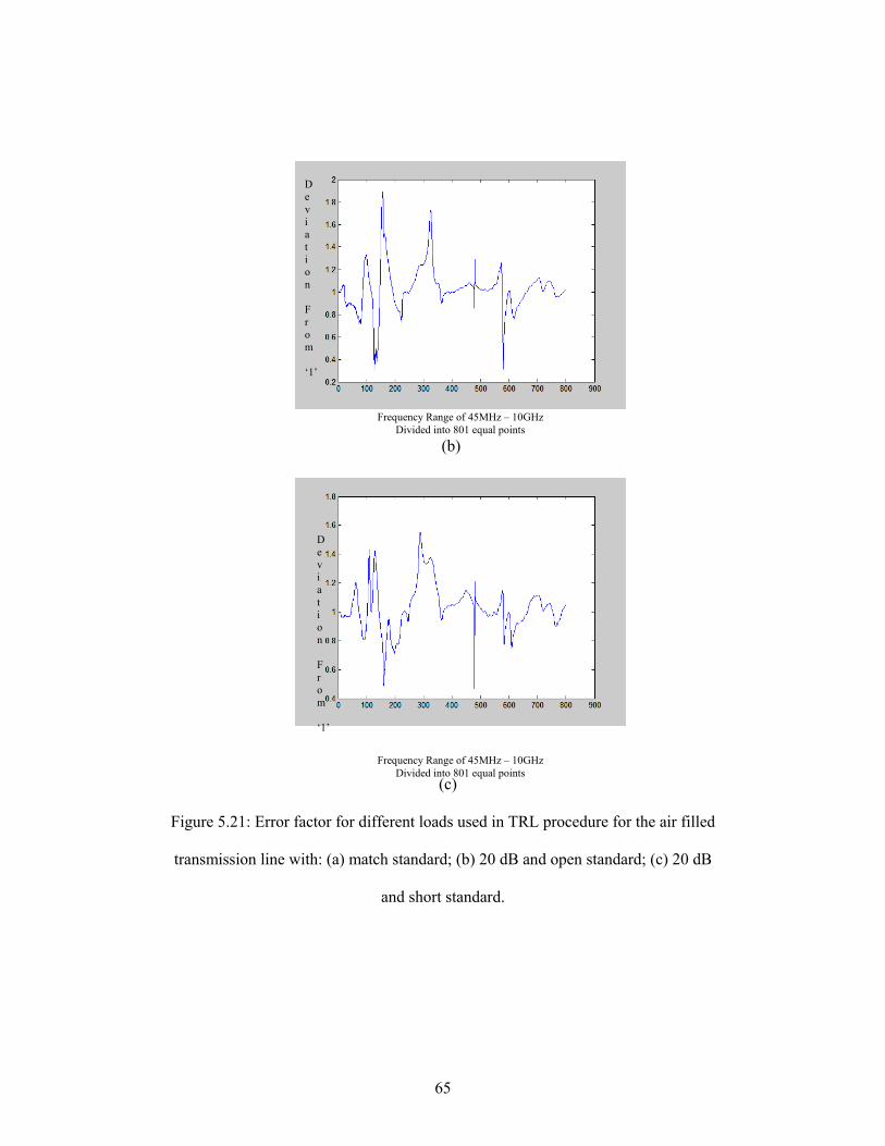
65
(b)
(c)
Figure 5.21: Error factor for different loads used in TRL procedure for the air filled
transmission line with: (a) match standard; (b) 20 dB and open standard; (c) 20 dB
and short standard.
D e v i a t i o n F r o m ‘1’
D e v i a t i o n F r o m ‘1’
Frequency Range of 45MHz – 10GHz Divided into 801 equal points
Frequency Range of 45MHz – 10GHz Divided into 801 equal points
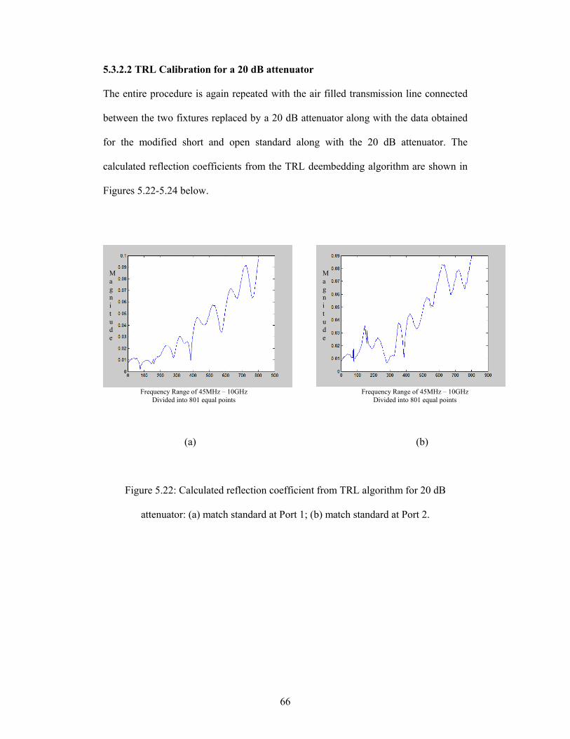
66
5.3.2.2 TRL Calibration for a 20 dB attenuator
The entire procedure is again repeated with the air filled transmission line connected
between the two fixtures replaced by a 20 dB attenuator along with the data obtained
for the modified short and open standard along with the 20 dB attenuator. The
calculated reflection coefficients from the TRL deembedding algorithm are shown in
Figures 5.22-5.24 below.
(a) (b)
Figure 5.22: Calculated reflection coefficient from TRL algorithm for 20 dB
attenuator: (a) match standard at Port 1; (b) match standard at Port 2.
Frequency Range of 45MHz – 10GHz Divided into 801 equal points
Frequency Range of 45MHz – 10GHz Divided into 801 equal points
M a g n i t u d e
M a g n i t u d e
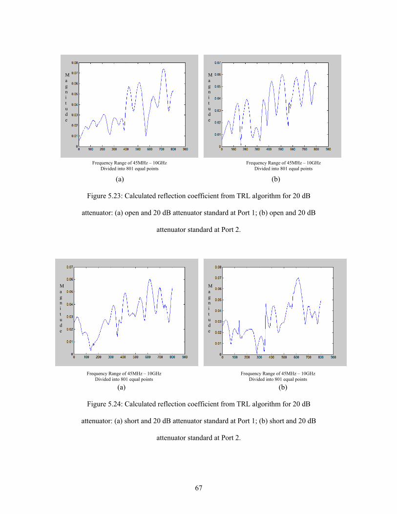
67
(a) (b)
Figure 5.23: Calculated reflection coefficient from TRL algorithm for 20 dB
attenuator: (a) open and 20 dB attenuator standard at Port 1; (b) open and 20 dB
attenuator standard at Port 2.
(a) (b)
Figure 5.24: Calculated reflection coefficient from TRL algorithm for 20 dB
attenuator: (a) short and 20 dB attenuator standard at Port 1; (b) short and 20 dB
attenuator standard at Port 2.
Frequency Range of 45MHz – 10GHz Divided into 801 equal points
Frequency Range of 45MHz – 10GHz Divided into 801 equal points
M a g n i t u d e
M a g n i t u d e
Frequency Range of 45MHz – 10GHz Divided into 801 equal points
Frequency Range of 45MHz – 10GHz Divided into 801 equal points
M a g n i t u d e
M a g n i t u d e
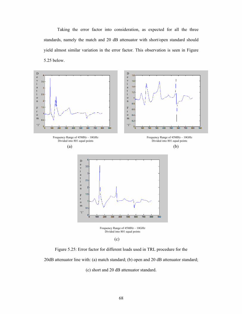
68
Taking the error factor into consideration, as expected for all the three
standards, namely the match and 20 dB attenuator with short/open standard should
yield almost similar variation in the error factor. This observation is seen in Figure
5.25 below.
(a) (b)
(c)
Figure 5.25: Error factor for different loads used in TRL procedure for the
20dB attenuator line with: (a) match standard; (b) open and 20 dB attenuator standard;
(c) short and 20 dB attenuator standard.
D e v i a t i o n F r o m ‘1’
D e v i a t i o n F r o m ‘1’
D e v i a t i o n F r o m ‘1’
Frequency Range of 45MHz – 10GHz Divided into 801 equal points
Frequency Range of 45MHz – 10GHz Divided into 801 equal points
Frequency Range of 45MHz – 10GHz Divided into 801 equal points
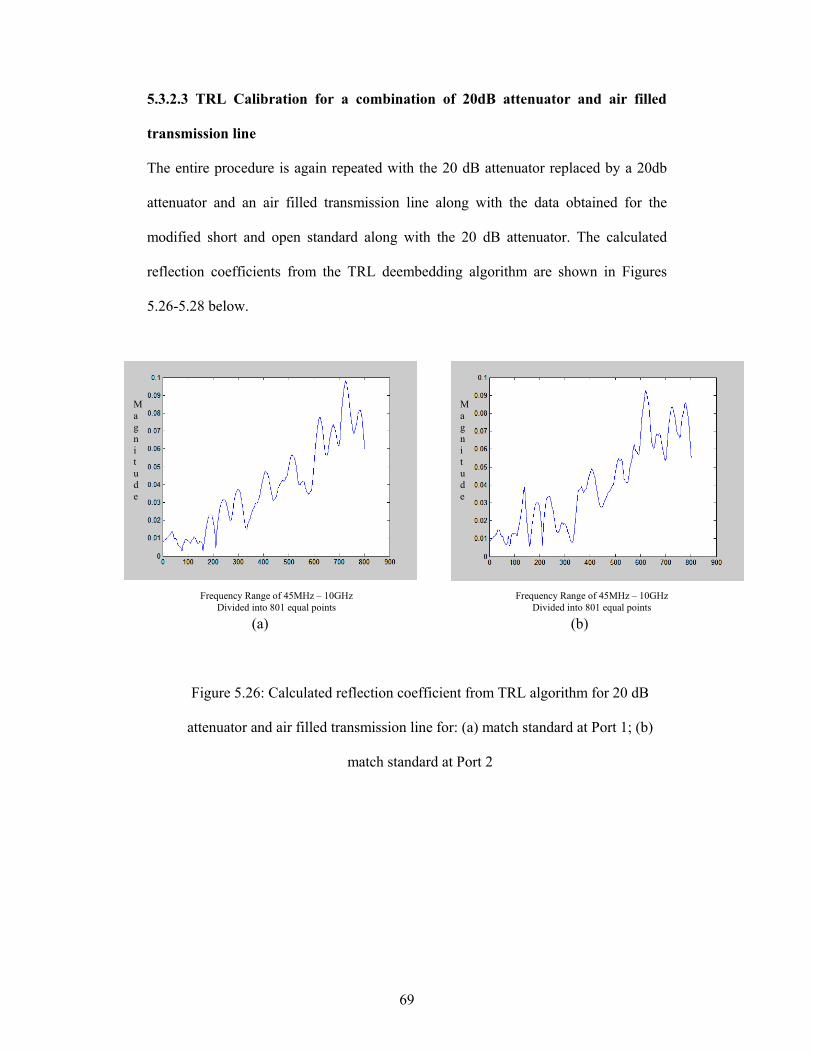
69
5.3.2.3 TRL Calibration for a combination of 20dB attenuator and air filled
transmission line
The entire procedure is again repeated with the 20 dB attenuator replaced by a 20db
attenuator and an air filled transmission line along with the data obtained for the
modified short and open standard along with the 20 dB attenuator. The calculated
reflection coefficients from the TRL deembedding algorithm are shown in Figures
5.26-5.28 below.
(a) (b)
Figure 5.26: Calculated reflection coefficient from TRL algorithm for 20 dB
attenuator and air filled transmission line for: (a) match standard at Port 1; (b)
match standard at Port 2
Frequency Range of 45MHz – 10GHz Divided into 801 equal points
Frequency Range of 45MHz – 10GHz Divided into 801 equal points
M a g n i t u d e
M a g n i t u d e
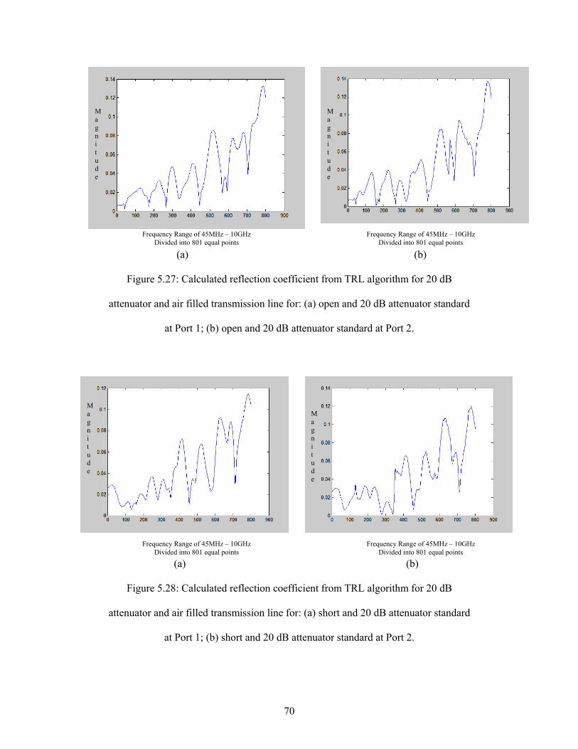
70
(a) (b)
Figure 5.27: Calculated reflection coefficient from TRL algorithm for 20 dB
attenuator and air filled transmission line for: (a) open and 20 dB attenuator standard
at Port 1; (b) open and 20 dB attenuator standard at Port 2.
(a) (b)
Figure 5.28: Calculated reflection coefficient from TRL algorithm for 20 dB
attenuator and air filled transmission line for: (a) short and 20 dB attenuator standard
at Port 1; (b) short and 20 dB attenuator standard at Port 2.
Frequency Range of 45MHz – 10GHz Divided into 801 equal points
Frequency Range of 45MHz – 10GHz Divided into 801 equal points
Frequency Range of 45MHz – 10GHz Divided into 801 equal points
Frequency Range of 45MHz – 10GHz Divided into 801 equal points
M a g n i t u d e
M a g n i t u d e
M a g n i t u d e
M a g n i t u d e
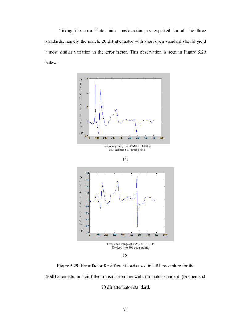
71
Taking the error factor into consideration, as expected for all the three
standards, namely the match, 20 dB attenuator with short/open standard should yield
almost similar variation in the error factor. This observation is seen in Figure 5.29
below.
(a)
(b)
Figure 5.29: Error factor for different loads used in TRL procedure for the
20dB attenuator and air filled transmission line with: (a) match standard; (b) open and
20 dB attenuator standard.
D e v i a t i o n F r o m ‘1’
D e v i a t i o n F r o m ‘1’
Frequency Range of 45MHz – 10GHz Divided into 801 equal points
Frequency Range of 45MHz – 10GHz Divided into 801 equal points
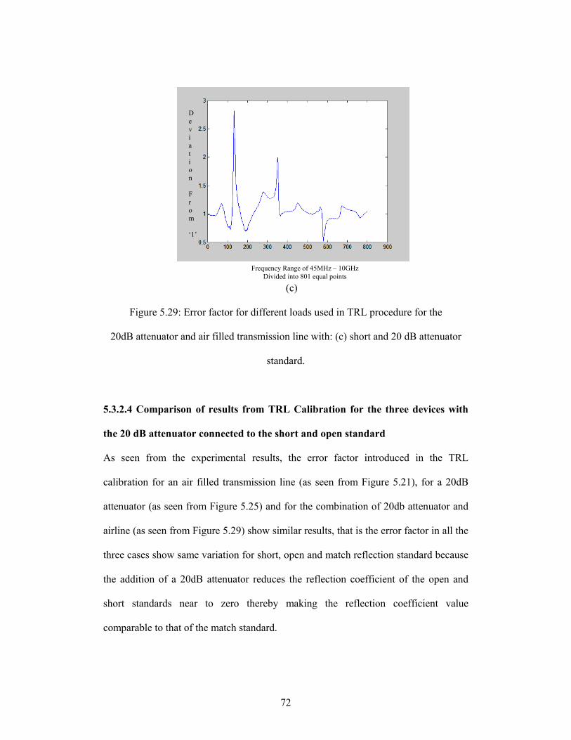
72
(c)
Figure 5.29: Error factor for different loads used in TRL procedure for the
20dB attenuator and air filled transmission line with: (c) short and 20 dB attenuator
standard.
5.3.2.4 Comparison of results from TRL Calibration for the three devices with
the 20 dB attenuator connected to the short and open standard
As seen from the experimental results, the error factor introduced in the TRL
calibration for an air filled transmission line (as seen from Figure 5.21), for a 20dB
attenuator (as seen from Figure 5.25) and for the combination of 20db attenuator and
airline (as seen from Figure 5.29) show similar results, that is the error factor in all the
three cases show same variation for short, open and match reflection standard because
the addition of a 20dB attenuator reduces the reflection coefficient of the open and
short standards near to zero thereby making the reflection coefficient value
comparable to that of the match standard.
D e v i a t i o n F r o m ‘1’
Frequency Range of 45MHz – 10GHz Divided into 801 equal points

73
Chapter 6: Conclusions
From the presented work, an important conclusion has been drawn on the selection of
the reflection standard required for accurate measurements. Apart from discussing the
theoretical analysis of the discrepancies caused due to variation in the reflection
coefficient seen at the two ports of the network analyzer, these discrepancies have
been verified and proved experimentally as well. From the experimental analysis, it is
also seen that similar variations in the measured data is obtained for TRL calibration
on three different test devices to further prove the validity of the analysis. The final
conclusion drawn is that the selection of short and open standard as the arbitrary
reflection standard in TRL calibration procedure will yield the highest accuracy and
the selection of match as the reflection standard will result in maximum inaccuracies
in the final measurements.
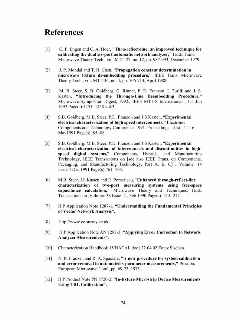
74
References
[1] G. F. Engen and C. A. Hoer, "Thru-refiect-line: an improved technique for calibrating the dual six-port automatic network analyzer," IEEE Trans. Microwave Theory Tech., vol. MTT-27, no. 12, pp. 987-993, December 1979.
[2] J. P. Mondal and T. H. Chen, "Propagation constant determination in microwave fixture de-embedding procedure," IEEE Trans. Microwave Theory Tech., vol. MTT-36, no. 4, pp. 706-714, April 1988.
[3] M. B. Steer, S. B. Goldberg, G. Rinnet, P. D. Franzon, I. Turlik and J. S. Kasten, “Introducing the Through-Line Deembedding Procedure,” Microwave Symposium Digest, 1992., IEEE MTT-S International , 1-5 Jun 1992 Page(s):1455 -1458 vol.3.
[4] S.B. Goldberg, M.B. Steer, P.D. Franzon and J.S Kasten, “Experimental
electrical characterization of high speed interconnects,” Electronic Components and Technology Conference, 1991. Proceedings., 41st , 11-16 May1991 Page(s): 85 -88.
[5] S.B. Goldberg, M.B. Steer, P.D. Franzon and J.S Kasten, “Experimental electrical characterization of interconnects and discontinuities in high-speed digital systems,” Components, Hybrids, and Manufacturing Technology, IEEE Transactions on [see also IEEE Trans. on Components, Packaging, and Manufacturing Technology, Part A, B, C] , Volume: 14 Issue:4 Dec 1991 Page(s):761 -765.
[6] M.B. Steer, J.S Kasten and R. Pomerleau, “Enhanced through-reflect-line characterization of two-port measuring systems using free-space capacitance calculation,” Microwave Theory and Techniques, IEEE Transactions on ,Volume: 38 Issue: 2 , Feb 1990 Page(s): 215 -217.
[7] H.P Application Note 1287-1, “Understanding the Fundamental Principles of Vector Network Analysis”.
[8] http://www.ee.surrey.ac.uk [9] H.P Application Note AN 1287-3, “Applying Error Correction to Network
Analyzer Measurements”.
[10] Characterization Handbook 1VNACAL.doc | 22.04.02 Franz Sischka. [11] N. R. Franzen and R. A. Spaciale, "A new procedure for system calibration
and error removal in automated s-parameter measurements," Proc. 5th
European Microwave Conf., pp. 69-73, 1975.
[12] H.P Product Note PN 8720-2, “In-fixture Microstrip Device Measurements Using TRL Calibration”.
75
[13] Jeffery S. Kasten, “Calibration of Automatic Network Analysis and Computer Aided Microwave Measurement,” Masters thesis, 1992.
[14] Dylan Williams, "De-embedding and Unterminating Microwave Fixtures with Nonlinear Least Squares," IEEE Trans. Microwave Theory Tech., vol. MTT-38, no. 6, pp. 787-791, June 1990.
[15] C. A. Hoer, "Performance of a Dual Six-port Automatic Network Analyzer," IEEE Trans. Microwave Theory Tech., vol. MTT-27, no. 12, pp. 993-998, December 1979.
[16] R. B. Marks, "A Multiline Method of Network Analyzer Calibration,"
IEEE Trans. Microwave Theory Tech., vol. MTT-39, no. 7, pp. 1205-1215, July 1991.
[17] D. F. Williams, R. B. Marks and A. Davidson, "Comparison of On-wafer
Calibrations," 38th ARFTG Conf. Dig., pp. 68-81, Dec 1991. [18] R. F. Kaiser and D. F. Williams, "Sources of Error in Coplanar-Waveguide
TRL Calibrations," National Institute of Standards and Technology.

76
Appendix A
Detailed TRL De-Embedding Solution
The calibration procedure consists of measuring the S matrices for the three standards,
namely Through, Reflect and Line which gives three known matrices. The three
matrices obtained give the scattering parameters of the fictitious two ports and the
scattering parameters of the individual error boxes A and B. The emergent wave
amplitudes b1, b2 at ports 1 and 2 are related to the incident waves a1, a2 by the well-
known scattering equations:
2121111 bSaSb += (A.1)
2221212 bSaSb += (A.2)
where the ijS are the scattering coefficients.
Dividing the first of these by al, the second by a2, and then eliminating the ratio al /a2
between them yields:
21222112 wwSwSw =∆−+ (A.3)
where
21122211 SSSS −=∆ (A.4)
The equation (3.5) shows the conversion between the T and the S parameters.
21
11
RR
22
12
RR
=
−
−−
21
22
21
11122211
SS
SSSSS
21
21
11
1S
SS
(A.5)
First convert the measured S parameters to their equivalent T parameters as in
equation (A.5). Let the cascading matrix be represented by the matrix R. Let the
cascading matrices of the error two-ports A and B be denoted by Ra and Rb

77
respectively, while Rt represents their cascade ‘thru’ connection and Rd represents the
cascade ‘Line’ measurements and Rl represents the cascade matrix of the inserted line.
Then
bat RRR = (A.6)
and,
blad RRRR 2= (A.7)
Solving (A.6) to get
ab RR = -1 tR (A.8)
Hence error matrix Rb can be obtained from the above equation.
Eliminating Rb in equation (A.6) we obtain the following
2laa RRTR =
Where: dRT = tR -1 (A.9)
or
-1
22 21
1211
tt tt
=
22M121M1
12M111M1
r rr r
22M2 21M2
12M211M2
r rr r
Where T matrix is represented by: T =
22 21
1211
tt tt
(A.10)
Rd matrix is represented by: Rd =
22M2 21M2
12M211M2
r rr r
(A.11)
and Rt matrix is represented by: Rt =
22M121M1
12M111M1
r rr r
(A.12)
Let Ra matrix be represented by: Ra =
22a21a
12a11a
r rr r
or Ra = ar22
ca
1b
(A.13)

78
where aa rra 2211 /= , aa rrb 2212 /= and aa rrc 2221 /= .
Let Rb matrix be represented by: Rb =
22b21b
12b11b
r rr r
or Rb = br 22
1
γ
βα (A.14)
where bb rr 2211 /=α , bb rr 2212 /=β and bb rr 2221 /=γ .
Hence equation (A.9) can also be written as -1
T =
22 21
1211
tt tt
=
22M121M1
12M111M1
r rr r
22M2 21M2
12M211M2
r rr r
(A.15)
Assuming that the line (represented by l 2) in non-reflecting, matrix Rd changes to
Rd =
22M121M1
12M111M1
r rr r
=
−0
)2( leExp γ
)2(
0leExp γ
Substituting the above mentioned matrix in equation (A.9) yields the following four
sets of equation:
errtrt aaaaa 1121121111 =+ -γl (A.16)
errtrt aaaaa 2121221121 =+ -γl (A.17)
errtrt aaaaa 1222121211 =+ -γl (A.18)
errtrt aaaaa 2222221221 =+ -γl (A.19)
Taking ratio of equation (A.16) to (A.17) and equation (A.18) to (3.19) yields
2 0)/)(()/( 1211111122111121 =−+ − aaaaaaaa trrttrrt (A.20)
2
0)/)(()/( 1222121122221221 =−+ − aaaaaaaa trrttrrt (A.21)
Ratio of equation (A.19) to (A.17) yields

79
eExp ( lγ2 ) = aaaa
aaaa
trrttrrt
11112112
22221221
)/()/(++ (A.22)
Hence from equations (A.20), (A.21) and (A.22), we have obtained three quantities:
=ca / )/( 2111 aa rr , =b )/( 2212 aa rr
and eExp ( lγ2 ) = aaaa
aaaa
trrttrrt
11112112
22221221
)/()/(++ (A.23)
The reflection coefficient w1 obtained at the fictitious port for the two port error A is
related to the reflection coefficient of the load by
1w = 1+Γ
+Γl
l
cba (A.24)
or
a = )/1( *1
1
acwbw
l −Γ− (A.25)
Similar analysis on the second two port error B yields
2w = 1+Γ−
−Γl
l
βγα (A.26)
or
α =)/1( *2
2
αβγ
ww
l +Γ− . (A.27)
The unknown reflection coefficient lΓ is eliminated from equation (A.25) and (A.27)
to yield
)]/1)(//[()])(/1)([( 221 aecacwbfdwbwa −+−+−±= γαβ (A.28)
Thus the need for the value of reflection coefficient to be exactly known is eliminated.
Once the value for ‘a’ for two port error matrix A is found, the remaining
parameters of the equation (A.13) and (A.14) can be found as follows:

80
From the ‘Thru’ and ‘Line’ measurements (A.23), the values for b and a/c have
already been obtained. Then from (A.6) substituting the matrix we get
r22a
1 c b a
* r22b
1
γ
βα = g
1 e
fd
(A.29)
where:
g
1 e
fd
= 22M1r
1 rr
rr rr 22M1 / 21M1
22M1 / 12M1 22M1 / 11M1
From (A.29) the following parameters can be easily obtained
γ = aecadcf
/1/
−− (A.30)
β/α = bfdbe
−− (A.31)
aα = aec
bfd/1−
− (A.32)
Hence from the above set of equations all the parameters of the 2 sets of error matrix
A and B can be found out. This entire procedure sums up the TRL solution for de-
embedding.
81
Appendix B
MATLAB Code for TRL Deembedding
% MATLAB Code for TRL Deembedding Solution % Author: Rahul Ghosh % Step 1: Reading Frequency for the Different Samples fid = fopen('frequency.txt','rt'); af = fscanf(fid,'%f',[1,900])' fclose(fid) % Step 2: Reading S Measurements for Through Standard fid = fopen('c_thru.txt','rt'); a9 = fscanf(fid,'%f %f',[2,3204])' fclose(fid) for i = 1:3204 a9_com(i) = complex(a9(i,1),a9(i,2)); end % Storing the S11 parameters for different frequencies for i = 1:801 S(1,i) = a9_com(i); end % Storing the S12 parameters for different frequencies for i = 1:801 S(2,i) = a9_com(1602+i); end % Storing the S21 parameters for different frequencies for i = 1:801 S(3,i) = a9_com(801+i); end % Storing the S22 parameters for different frequencies for i = 1:801 S(4,i) = a9_com(2403+i); end
82
% Step 3: Convert reading from S to T parameters for further processing. % S11 conversion for i = 1:801 Rt1_t(1,i) = -((S(1,i)* S(4,i) - S(2,i)*S(3,i))/S(3,i)) end % S12 conversion for i = 1:801 Rt1_t(2,i) = S(1,i)/S(3,i) end % S21 conversion for i = 1:801 Rt1_t(3,i) = - S(4,i)/S(3,i) end % S22 conversion for i = 1:801 Rt1_t(4,i) = 1/S(3,i) end % Step 4: Reading files for different sets of measurements and storing them % appropriately. fid = fopen('20db_attn_line.txt','rt'); b1 = fscanf(fid,'%f %f',[2,3204])' fclose(fid) for i = 1:3204 b1_com(i) = complex(b1(i,1),b1(i,2)); end for i = 1:801 S1(1,i) = b1_com(i); end for i = 1:801 S1(2,i) = b1_com(1602+i); end for i = 1:801 S1(3,i) = b1_com(801+i); end for i = 1:801 S1(4,i) = b1_com(2403+i); end
83
% Convert from S to T parameters for further processing % S11 conversion for i = 1:801 Rd_t(1,i) = -((S1(1,i)* S1(4,i) - S1(2,i)*S1(3,i))/S1(3,i)) end % S12 conversion for i = 1:801 Rd_t(2,i) = S1(1,i)/S1(3,i) end % S21 conversion for i = 1:801 Rd_t(3,i) = - S1(4,i)/S1(3,i) end % S22 conversion for i = 1:801 Rd_t(4,i) = 1/S1(3,i) end % Reading files for Matched load for side 1 fid = fopen('c_m1.txt','rt'); a1 = fscanf(fid,'%f %f',[2,900])' fclose(fid) for i = 1:801 a1_com(i) = complex(a1(i,1),a1(i,2)); end for i = 1:801 Sm(1,i) = a1_com(i); end % Reading files for Matched load for side 2 fid = fopen('c_m2.txt','rt'); a2 = fscanf(fid,'%f %f',[2,900])' fclose(fid) for i = 1:801 a2_com(i) = complex(a2(i,1),a2(i,2)); end for i = 1:801 Sm2(1,i) = a2_com(i); end % Reading files for SHORT load for side 1 fid = fopen('s501.txt','rt'); a3 = fscanf(fid,'%f %f',[2,900])' fclose(fid) for i = 1:801
84
a3_com(i) = complex(a3(i,1),a3(i,2)); end for i = 1:801 Ss1(1,i) = a3_com(i); end % Reading files for SHORT load for side 2 fid = fopen('s502.txt','rt'); a4 = fscanf(fid,'%f %f',[2,900])' fclose(fid) for i = 1:801 a4_com(i) = complex(a4(i,1),a4(i,2)); end for i = 1:801 Ss2(1,i) = a4_com(i); end % Reading files for OPEN load for side 1 fid = fopen('o501.txt','rt'); a5 = fscanf(fid,'%f %f',[2,900])' fclose(fid) for i = 1:801 a5_com(i) = complex(a5(i,1),a5(i,2)); end for i = 1:801 So1(1,i) = a5_com(i); end % Reading files for OPEN load for side 2 fid = fopen('o502.txt','rt'); a6 = fscanf(fid,'%f %f',[2,900])' fclose(fid) for i = 1:801 a6_com(i) = complex(a6(i,1),a6(i,2)); end for i = 1:801 So2(1,i) = a6_com(i); end % Step 5: Begin TRL Deembedding algorithm according to [1]. i = 1 while (i <= 801) for j=1:2 for k =1:2 Rt1(j,k) = Rt1_t((j-1)*2+k,i) Rd(j,k) = Rd_t((j-1)*2+k,i) end end

85
RM1_s(i) = Sm(1,i) RM2_s(i) = Sm2(1,i) RS1_s(i) = Ss1(1,i) RS2_s(i) = Ss2(1,i) Ro1_s(i) = So1(1,i) Ro2_s(i) = So2(1,i) % Calculation of the reflection coefficient ‘w1 and w2’ for the calculation of 'a' % Refer to w1 and w2 in [1] % For MATCH standard rc_m1(i) = RM1_s(i) % w1 rc_m2(i) = RM2_s(i) % w2 rc_m1_mag(i) = abs(rc_m1(i)) rc_m2_mag(i) = abs(rc_m2(i)) rc_m1_phase(i) = angle(rc_m1(i)) rc_m2_phase(i) = angle(rc_m2(i)) % For SHORT standard rc_s1(i) = RS1_s(i) rc_s2(i) = RS2_s(i) rc_s1_phase(i) = angle(rc_s1(i)) rc_s2_phase(i) = angle(rc_s2(i)) rc_s1_mag(i) = abs(rc_s1(i)) rc_s2_mag(i) = abs(rc_s2(i)) % For OPEN standard rc_o1(i) = Ro1_s(i) rc_o2(i) = Ro2_s(i) rc_o1_mag(i) = abs(rc_o1(i)) rc_o2_mag(i) = abs(rc_o2(i)) rc_o1_phase(i) = angle(rc_o1(i)) rc_o2_phase(i) = angle(rc_o2(i)) % Further processing, please refer [1] T = Rd * inv(Rt1) % Storing the data for solving the quadratic equation. a_eq(i) = T(2,1) b_eq(i) = (T(2,2) - T(1,1)) c_eq(i) = T(1,2)
86
% Calculating the roots for solving the quadratic equation. root1(i) = (((-b_eq(i))+(((b_eq(i)^2)-(4*a_eq(i)*c_eq(i)))^(1/2)))/(2*a_eq(i))) root2(i) = (((-b_eq(i))-(((b_eq(i)^2)-(4*a_eq(i)*c_eq(i)))^(1/2)))/(2*a_eq(i))) % Selecting the right roots values for which abs (b) < abs (a/c) root1_mag(i) = abs(root1(i)) % = 0.4449 root2_mag(i) = abs(root2(i)) % = 2.5931 if (root1_mag(i) < root2_mag(i)) b(i) = root1(i) a_c(i) = root2(i) else b(i) = root2(i) a_c(i) = root1(i) end % Removing the ‘through 22’ element outside the matrix Rt = Rt1/Rt1(2,2) % Rt 'one' % Calculations for the error box B % Notations same as those used in [1] d(i) = Rt(1,1) e(i) = Rt(1,2) f(i) = Rt(2,1) gamma(i) = (f(i) - (d(i)*(1/a_c(i))))/(1 - e(i)*(1/a_c(i))) beta_alpha(i) = (e(i) - b(i))/(d(i)-(b(i)*f(i))) a_alpha(i) = (d(i) - (b(i)*f(i)))/(1-(e(i)*(1/a_c(i)))) % Estimation in the value of 'a' for different loads % For Match condition a_matched_wo_error(i) = sqrt(((rc_m1(i) - b(i))*(1 + rc_m2(i)* beta_alpha(i))*(d(i) - b(i)*f(i)))/((rc_m2(i) + gamma(i))*(1 - rc_m1(i)*(1/a_c(i)))*(1-e(i)*(1/a_c(i))))) % For Short condition a_short_wo_error(i) = sqrt(((rc_s1(i) - b(i))*(1 + rc_s2(i)* beta_alpha(i))*(d(i) - b(i)*f(i)))/((rc_s2(i) + gamma(i))*(1 - rc_s1(i)*(1/a_c(i)))*(1-e(i)*(1/a_c(i))))) % For Open condition a_open_wo_error(i) = sqrt(((rc_o1(i) - b(i))*(1 + rc_o2(i)* beta_alpha(i))*(d(i) - b(i)*f(i)))/((rc_o2(i) + gamma(i))*(1 - rc_o1(i)*(1/a_c(i)))*(1-e(i)*(1/a_c(i)))))
87
% Step 6: Calculations taking into considerations the proposed error factor % First Estimate the variation in the value of Reflection Co-efficient seen at the two % ports. % To find the error value you will need to find the reflection coefficient 1 and 2 with % values w1 and w2 and then subtract them to find error. % Reflection co-efficient of side 1. % For match standard reflection_coef_m1(i) = ((rc_m1(i) - b(i))/(a_matched_wo_error(i)*(1 - (rc_m1(i)*1/a_c(i))))) % For short standard reflection_coef_s1(i) = ((rc_s1(i) - b(i))/(-a_short_wo_error(i)*(1 + (rc_s1(i)*1/a_c(i))))) % changed % For open standard reflection_coef_o1(i) = ((rc_o1(i) - b(i))/(a_open_wo_error(i)*(1 - (rc_o1(i)*1/a_c(i))))) reflection_coef_m1_mag(i) = abs(reflection_coef_m1(i)) reflection_coef_s1_mag(i) = abs(reflection_coef_s1(i)) reflection_coef_o1_mag(i) = abs(reflection_coef_o1(i)) % Reflection co-efficient of side 2 % For match standard reflection_coef_m2(i) = ((rc_m2(i) - b(i))/(a_matched_wo_error(i)*(1 - (rc_m2(i)*1/a_c(i))))) % For short standard reflection_coef_s2(i) = ((rc_s2(i) - b(i))/(-a_short_wo_error(i)*(1 + (rc_s2(i)*1/a_c(i))))) % For open standard reflection_coef_o2(i) = ((rc_o2(i) - b(i))/(a_open_wo_error(i)*(1 - (rc_o2(i)*1/a_c(i))))) reflection_coef_m2_mag(i) = abs(reflection_coef_m2(i)) reflection_coef_s2_mag(i) = abs(reflection_coef_s2(i)) reflection_coef_o2_mag(i) = abs(reflection_coef_o2(i))

88
% Error factor calculations % For match, short and open standards. error_m(i) = (reflection_coef_m1(i) - reflection_coef_m2(i)) error_s(i) = (reflection_coef_s1(i) - reflection_coef_s2(i)) error_o(i) = (reflection_coef_o1(i) - reflection_coef_o2(i)) % The variation in the value of ‘a’ from the accurate measurement for different % standards used, namely match, open and short. a_varies_by_m(i) = sqrt(1+(error_m(i)/(reflection_coef_m1(i)))) a_varies_by_o(i) = sqrt(1+(error_o(i)/(reflection_coef_o1(i)))) a_varies_by_s(i) = sqrt(1+(error_s(i)/(reflection_coef_s1(i)))) a_varies_by_m_mag(i) = abs(a_varies_by_m(i)) a_varies_by_s_mag(i) = abs(a_varies_by_s(i)) a_varies_by_o_mag(i) = abs(a_varies_by_o(i)) % The value ‘i’ traverses through the 801 set of readings for different frequencies. i=i+1 end