MANIPULATION AND SEPARATION OF OBJECTS ATTHE MICROSCALE, IN SOLUTION AND AT

INTERFACES

By

Harsh Pandey

A Dissertation Submitted to the Graduate

Faculty of Rensselaer Polytechnic Institute

in Partial Fulfillment of the

Requirements for the Degree of

DOCTOR OF PHILOSOPHY

Major Subject: CHEMICAL AND BIOLOGICAL ENGINEERING

Examining Committee:

Prof. Patrick T. Underhill, Dissertation Adviser

Prof. Shekhar Garde, Member

Prof. Joel L. Plawsky, Member

Prof. Chang Y. Ryu, Member

Rensselaer Polytechnic InstituteTroy, New York

July 2015(For Graduation August 2015)

c© Copyright 2015

by

Harsh Pandey

All Rights Reserved

ii

CONTENTS

LIST OF TABLES . . . . . . . . . . . . . . . . . . . . . . . . . . . . . . . . . v

LIST OF FIGURES . . . . . . . . . . . . . . . . . . . . . . . . . . . . . . . . vi

ACKNOWLEDGMENTS . . . . . . . . . . . . . . . . . . . . . . . . . . . . . ix

ABSTRACT . . . . . . . . . . . . . . . . . . . . . . . . . . . . . . . . . . . . x

1. MOTIVATION AND OBJECTIVES . . . . . . . . . . . . . . . . . . . . . 1

1.1 Motivation . . . . . . . . . . . . . . . . . . . . . . . . . . . . . . . . . 1

1.2 Objectives . . . . . . . . . . . . . . . . . . . . . . . . . . . . . . . . . 4

2. BACKGROUND . . . . . . . . . . . . . . . . . . . . . . . . . . . . . . . . 6

2.1 DNA Electrophoresis . . . . . . . . . . . . . . . . . . . . . . . . . . . 6

2.2 Field-Flow Fractionation . . . . . . . . . . . . . . . . . . . . . . . . . 11

2.3 Microfluidics for Trapping and Manipulation . . . . . . . . . . . . . . 13

2.4 Manipulating Polymers at Aqueous Interfaces . . . . . . . . . . . . . 14

3. COARSE-GRAINEDMODELOF CONFORMATION-DEPENDENT ELEC-TROPHORETIC MOBILITY . . . . . . . . . . . . . . . . . . . . . . . . . 17

3.1 Introduction . . . . . . . . . . . . . . . . . . . . . . . . . . . . . . . . 17

3.2 Model Development . . . . . . . . . . . . . . . . . . . . . . . . . . . . 18

3.2.1 Hydrodynamic versus electrohydrodynamic interactions . . . . 18

3.2.2 Conformation-dependent mobility . . . . . . . . . . . . . . . . 22

3.3 Simulation Methodology . . . . . . . . . . . . . . . . . . . . . . . . . 26

3.4 Model Verification . . . . . . . . . . . . . . . . . . . . . . . . . . . . 31

3.4.1 Straight channel migration . . . . . . . . . . . . . . . . . . . . 31

3.4.2 Stretching in an electric field gradient . . . . . . . . . . . . . . 34

3.5 Conclusions . . . . . . . . . . . . . . . . . . . . . . . . . . . . . . . . 38

4. SIMULATIONS OF TRAPPING ANDMANIPULATION OFDEFORMABLEOBJECTS . . . . . . . . . . . . . . . . . . . . . . . . . . . . . . . . . . . . 40

4.1 Trapping Objects in Confined Microfluidic Geometries . . . . . . . . 40

4.2 Manipulating Objects in Unconfined Flows and Fields . . . . . . . . . 44

4.3 Conclusions . . . . . . . . . . . . . . . . . . . . . . . . . . . . . . . . 49

iii

5. SIMULATIONS OF TRAPPING ANDMANIPULATION OF RIGID ORI-ENTABLE OBJECTS . . . . . . . . . . . . . . . . . . . . . . . . . . . . . 50

5.1 Introduction . . . . . . . . . . . . . . . . . . . . . . . . . . . . . . . . 50

5.2 Rigid Rod Model . . . . . . . . . . . . . . . . . . . . . . . . . . . . . 50

5.3 Stable Trapping Using Electric and Flow Fields . . . . . . . . . . . . 52

5.4 Conclusions . . . . . . . . . . . . . . . . . . . . . . . . . . . . . . . . 55

6. MICROFLUIDICS EXPERIMENTS . . . . . . . . . . . . . . . . . . . . . 56

6.1 Channel Preparation . . . . . . . . . . . . . . . . . . . . . . . . . . . 56

6.2 Microscopy, Imaging and Data Analysis . . . . . . . . . . . . . . . . . 58

6.3 Observations At Equilibrium . . . . . . . . . . . . . . . . . . . . . . . 59

6.4 Observations under Fluid Flow . . . . . . . . . . . . . . . . . . . . . 60

6.5 Observations under Electric Field . . . . . . . . . . . . . . . . . . . . 62

6.6 Conclusions . . . . . . . . . . . . . . . . . . . . . . . . . . . . . . . . 67

7. SIMULATIONS OF THE MANIPULATION OF POLYMERS AT AQUE-OUS INTERFACES . . . . . . . . . . . . . . . . . . . . . . . . . . . . . . 69

7.1 Introduction . . . . . . . . . . . . . . . . . . . . . . . . . . . . . . . . 69

7.2 Simulation Methodology . . . . . . . . . . . . . . . . . . . . . . . . . 71

7.3 Quantifying the Effect of Polymer Concentration on Self-Assembly . . 74

7.4 Conclusions . . . . . . . . . . . . . . . . . . . . . . . . . . . . . . . . 77

8. IMPACT AND FUTURE DIRECTIONS . . . . . . . . . . . . . . . . . . . 78

APPENDICES

A. Calculation of Wall-Mediated Hydrodynamic Interactions . . . . . . . . . . 80

A.1 Blake’s solution for a point force near an infinite plane wall with no-slip 81

A.2 Hydrodynamic diffusion tensor for a bead-spring polymer betweentwo walls . . . . . . . . . . . . . . . . . . . . . . . . . . . . . . . . . . 82

REFERENCES . . . . . . . . . . . . . . . . . . . . . . . . . . . . . . . . . . . 85

iv

LIST OF TABLES

6.1 Uncharged microspheres in the straight channel with an applied electricfield . . . . . . . . . . . . . . . . . . . . . . . . . . . . . . . . . . . . . . 64

6.2 Electrophoresis of charged microspheres in the straight channel . . . . . 64

6.3 DNA electrophoresis in a straight channel . . . . . . . . . . . . . . . . . 65

6.4 Electrophoresis of charged microspheres in a T-channel . . . . . . . . . 66

v

LIST OF FIGURES

1.1 Illustration of the principle of conformation-dependent electrophoreticmobility. . . . . . . . . . . . . . . . . . . . . . . . . . . . . . . . . . . . 1

2.1 Schematic illustration of the local electrostatics around a DNA coil . . . 7

2.2 Illustration of electro-hydrodynamic interactions (EHI) that occur dur-ing electrophoresis. . . . . . . . . . . . . . . . . . . . . . . . . . . . . . 8

2.3 Distribution of electrophoretic mobility of λ-phage DNA versus DNAvisual length. . . . . . . . . . . . . . . . . . . . . . . . . . . . . . . . . . 10

2.4 Cross-channel migration of λ-phage DNA in capillary electrophoresis . . 12

2.5 (a) Hydrodynamic trap created by a planar extensional flow field atthe junction of two perpendicular microchannels. (b) The velocity field(top) and the velocity potential well (bottom) for a particle in the flowfield at the microchannel junction. . . . . . . . . . . . . . . . . . . . . . 14

3.1 Schematic of a linear polymer in a coiled (near equilibrium) and ex-tended conformation. . . . . . . . . . . . . . . . . . . . . . . . . . . . . 19

3.2 Coarse-graining a series of Kuhn segments with an equivalent bead-spring dumbbell. . . . . . . . . . . . . . . . . . . . . . . . . . . . . . . . 22

3.3 Capillary electrophoresis (rectangular channel) with pressure-driven flowshowing co-current migration across the streamlines. . . . . . . . . . . . 32

3.4 Capillary electrophoresis (rectangular channel) with pressure-driven flowshowing counter-current migration across the streamlines. . . . . . . . . 32

3.5 Scatter plot of the chain stretch of ds-DNA as a function of the Henckystrain. . . . . . . . . . . . . . . . . . . . . . . . . . . . . . . . . . . . . 35

3.6 Scatter plot of the electrophoretic mobility of ds-DNA as a function ofthe chain stretch for WiE = 3. . . . . . . . . . . . . . . . . . . . . . . . 36

3.7 Scatter plot of the electrophoretic mobility of ds-DNA as a function ofthe chain stretch for WiE = 30. . . . . . . . . . . . . . . . . . . . . . . 36

3.8 Scatter plot of the electrophoretic mobility of ds-DNA as a function ofthe chain stretch for WiE = 90. . . . . . . . . . . . . . . . . . . . . . . 37

4.1 Simulation of a polymer in a T-channel with Wi = 2 and WiE = −3.96. 42

vi

4.2 Combined flow and field streamlines in a Cross channel with Wi = 2and WiE = −3.96. . . . . . . . . . . . . . . . . . . . . . . . . . . . . . . 43

4.3 Simulation of a polymer in an ideal combination of an elongationalelectric field and fluid flow. Position of the center of mass plotted as afunction of time. . . . . . . . . . . . . . . . . . . . . . . . . . . . . . . . 45

4.4 Simulation of a polymer in an ideal combination of an elongationalelectric field and fluid flow. The stretch of the molecules plotted as afunction of time. . . . . . . . . . . . . . . . . . . . . . . . . . . . . . . . 46

4.5 Polymer dumbbell in a combination of elongational electric field andfluid flow . . . . . . . . . . . . . . . . . . . . . . . . . . . . . . . . . . . 46

4.6 Residence time of polymer and rigid sphere plotted versus trajectorynumber for Wi = 12.24,W i+WiE = 2 . . . . . . . . . . . . . . . . . . 48

5.1 Trapping of a rigid rod in an elongational flow and field. . . . . . . . . . 53

5.2 Trapping of a rigid rod in an elongational flow and field. . . . . . . . . . 54

5.3 Trapping of a rigid rod in an elongational flow and field. . . . . . . . . . 54

6.1 Schematic illustration of ‘Replica Molding’. . . . . . . . . . . . . . . . . 56

6.2 Illustration of some of the experimental methods used. . . . . . . . . . . 58

6.3 Plot of mean-squared displacement as a function of lag time for 1µmdiameter carboxylated Polystyrene microspheres visualized at equilibrium. 60

6.4 Streaklines of Polystyrene microspheres in fluid flow in a T-channel . . . 62

6.5 Streaklines of Polystyrene microspheres in electric field in a T-channel . 67

7.1 PMF between pairs of homopolymers at the vapor-liquid interface. . . . 70

7.2 PMF between pairs of homopolymers in bulk water. . . . . . . . . . . . 70

7.3 Radial distribution function g(r) versus bead separation (r/L) for the2-D Brownian dynamics simulation of polymers at a vapor-liquid interface. 73

7.4 Verification of the BD Simulation: Fitting the pair correlation functionto the Boltzmann distribution of the applied potential . . . . . . . . . . 73

7.5 Homopolymer simulations in bulk water . . . . . . . . . . . . . . . . . . 75

7.6 Homopolymer simulations at the vapor-liquid interface . . . . . . . . . . 75

7.7 VMD snapshot of the system of homopolymers at the vapor-liquid in-terface . . . . . . . . . . . . . . . . . . . . . . . . . . . . . . . . . . . . 76

vii

7.8 VMD snapshot of the system of homopolymers at the vapor-liquid in-terface . . . . . . . . . . . . . . . . . . . . . . . . . . . . . . . . . . . . 76

7.9 VMD snapshot of the system of homopolymers at the vapor-liquid in-terface . . . . . . . . . . . . . . . . . . . . . . . . . . . . . . . . . . . . 76

A.1 Illustration of a point force and its image near an infinite plane wall. . . 80

A.2 Illustration of a polymer dumbbell and its images in the two walls . . . 83

viii

ACKNOWLEDGMENTS

I thank my advisor Professor Patrick T. Underhill for his guidance, patience

and support. He has played a major role in the development of this thesis and kept

me motivated throughout my graduate studies.

I am grateful to my doctoral committee members Professor Shekhar Garde,

Professor Joel L. Plawsky and Professor Chang Y. Ryu. They have provided feed-

back, asked insightful questions and helped me whenever I contacted them.

I would like to thank Professor Garde’s group for collaboration on the interface

simulations. I thank the services of Mr. Robert Healey, who has assisted us in

maintaining our computer cluster. I also thank the Engineers at the RPI Cleanroom,

Mr. Bryant Colwill and Dr. Kent Way, for their technical assistance. I am thankful

to Rose Primett, Lee Vilardi, Sharon Sorell and Jennifer Krausnick who have helped

me and other graduate students in the CBE department in many ways.

I am grateful to my mentors during my undergraduate studies, who have in-

spired me to pursue graduate studies. My thanks to Professor R.P. Singh, Professor

Pramod Kumar and Professor P.K. Kamani from HBTI.

My research group members have helped me with great discussions and have

also been fun to work with. Special thanks to Dr. Rangarajan Radhakrishnan, Dr.

Sandeep Chilukuri, Dr. Yaser Bozorgi and Dr. Suhas Rao. I also thank Purba

Chatterjee, Yuzhou Qian and Edmund Tang for their support.

I had the privilege of mentoring several undergraduate students on my re-

search. Thanks to Michael McIntyre, Hannah Clough, Sylvia Szafran and Seth

Ludwig.

Heartfelt thanks to my brother Dhruv, parents Vijay and Mala Pandey, rela-

tives and friends for being there for me all the way.

ix

ABSTRACT

Many separation techniques rely on different physical or chemical character-

istics of the objects being separated. This includes separations based on size, total

charge, or strength of interaction with a substrate. Recently there are many con-

texts in which it is important to manipulate or separate objects with much more

subtle differences. For example, there has been significant interest in separating

cells with different deformabilities because disease states can lead to changes in flex-

ibility or stiffness, as observed in the red blood cells in sickle cell anemia. Proteins

are another example in which manipulating molecules based on their flexibility or

deformability (e.g. due to unfolding or di-sulfide bonds) is currently challenging.

Further, genomic-length DNA separation and manipulation has direct applications

in the development of novel DNA mapping and sequencing devices.

Apart from manipulating objects in solution in the cases above, it is also in-

teresting to study the self-assembly of objects at interfaces. Interface mediated

self-assembly of practical interest includes many solutes interacting to form aggre-

gates with internal structures (e.g., fibrils), coatings (e.g., films of heteropolymers

or unfolded proteins), and other larger structures of technological interest forming

over larger time-scales.

With these broad guides in mind, the overarching goal of our work is to gain

a better understanding of the manipulation and separation of objects at the mi-

croscale, both in solution as well as at an interface. The key principle underlying

most of our work is the conformation-dependent electrophoretic mobility of the ob-

ject; as the object changes its conformation, the mobility changes, which leads to a

different electrophoretic velocity and response to electric field gradients.

x

We have developed a computational model that can efficiently simulate the dy-

namics of rigid as well as flexible objects in a combination of electric field gradients

and pressure driven flow, and have used this model to show that conformation-

dependent electrophoretic mobility can be used to trap and manipulate objects. We

are interested in using the predictions from the simulations to design microfluidic

devices to trap and manipulate deformable objects. The interplay between the elec-

tric field and the fluid flow in the microchannels, given the coupled dynamics of

the effective field on these objects and their conformation, can allow for manipula-

tion and stretching in a unique way. We have extended the technique to perform

simulations of the manipulation and trapping of rod-like objects such as Tobacco

Mosaic Virus (TMV). Apart from looking at objects in solution, we have examined

the structure and dynamics of polymers at aqueous interfaces through Brownian

dynamics simulations.

xi

1. MOTIVATION AND OBJECTIVES

1.1 Motivation

The overarching goal of our work is to gain a better understanding of the ma-

nipulation and separation of objects at the microscale, both in solution as well as

at an interface. The key principle underlying most of our work is the conformation-

dependent electrophoretic mobility of the object; as the object changes its confor-

mation, the mobility changes, which leads to a different electrophoretic velocity and

response to electric field gradients.

This principle is illustrated in Figure 1.1. When both a fluid flow and an

electric field are applied, an object sees the net effect of the fluid velocity v and

the mobility dotted into the electric field µ·E. Fluid flow gradients or electric field

gradients can cause the object to deform, which changes µ and the balance between

v and µ·E.

Many separation techniques rely on different physical or chemical character-

istics of the objects being separated. This includes separations based on size, total

Figure 1.1: Illustration of of the principle of conformation-dependent electrophoreticmobility. (a) For a rigid object or a coiled polymer, the object sees thenet effect of the fluid flow v and the electric field contribution µ·E. (b)When a deformable object stretches, the mobility µ will change andtherefore changes the balance between the fluid flow and electric fieldcontributions.

1

2

charge, or strength of interaction with a substrate. Recently there are many contexts

in which it is important to manipulate or separate objects with much more subtle

differences. For example, there has been significant interest in separating cells with

different deformabilities because disease states can lead to changes in flexibility or

stiffness, as observed in the red blood cells in sickle cell anemia. Proteins are another

example in which manipulating molecules based on their flexibility or deformability

(e.g. due to unfolding or di-sulfide bonds) is currently challenging. In our approach,

an electric field gradient is combined with a pressure driven flow. If the object is

deformable or orientable, the change in conformation will change the electrophoretic

mobility, which in turn changes how fast the object moves and is deformed. This

is one example in which the deformation of flexible polymers is important in practice.

Dilute solutions of flexible polymers are not only interesting from a theoretical

standpoint, but also have practical applications such as in enhanced oil recovery [1]

and turbulent drag reduction [2]. From a biological standpoint, it is also known that

flow properties of proteins can serve important biological functions [3–5]. Macro-

scopic properties of polymer solutions are determined by their microstructure [6,7].

Direct observations of double stranded DNA (ds-DNA) have successfully verified

the connection of flow behavior with microstructure [8–14].

Microfluidic [15] systems can replace many conventional macroscale systems

because of their low input of samples and reagents, ability to manipulate small

volumes and high speed of reactions and separations. Further, the processes in mi-

crofluidic systems are conducted at scales more relevant to biological conditions (e.g.

at a size of a single cell). Research is progressing towards a Micro-Total Analysis

System (µTAS), popularly known as a Lab-on-a-chip, which integrates sampling,

3

sample preparation and transport, chemical reactions, and detection in a single

miniaturized platform [16–19]. As an example, microfluidic platforms for single-cell

analysis [20] enable cell manipulation such as cell sorting, performing controlled cell

lysis and chemical reactions in a single chip.

The mapping and sequencing of genomic-length DNA, essentially the reading

of the sequence of the base pairs, is important for the diagnosis of genetic diseases,

genome engineering, forensic science etc. Novel and futuristic applications such

as DNA computing [21] and digital information storage in DNA [22] demand ever

faster DNA sequencing. Gel electrophoresis [23, 24] is currently the workhorse for

mapping of DNA, with Pulsed Field Gel Electrophoresis (PFGE) [25] used regularly

for fragments greater than tens of kilo-base pair(Kbp). Although PFGE involves

low cost and easy protocol, yet it leads to relatively long times for analysis (e.g.

PFGE of Mbp DNA (Yeast chromosome) can take hours to days) [26]. Micro-fluidic

and nano-fluidic DNA manipulation and separation methods aim to circumvent this

limitation, additionally offering easier opportunities to integrate related analytical

techniques to form a lab-on-a-chip [26].

Apart from manipulating objects in solution, it is also interesting to study

the self-assembly of objects at interfaces. Self-assembly plays an important role in

natural processes and technologies used to make new materials. A key goal in stud-

ies of self-assembly is to better understand how the interactions of the constituents

lead to the self-assembled structures, and their underlying properties. Structure

and dynamics of water molecules are significantly affected by the presence of in-

terfaces, which has been observed in simulations and experiments [27–30]. How

those changes influence water-mediated interactions, and consequently, how inter-

4

faces mediate self-assembly in their vicinity is however not understood. As a relevant

example of assembly being influenced by a hydrophobic interface, the lag time in

the fibril formation of Alzheimer’s A-β protein fragments was found to be decreased

significantly in the presence of hydrophobic nanoparticles [31], vapor-liquid inter-

faces, or Teflon beads [32]. Interface mediated self-assembly of practical interest

includes many solutes interacting to form aggregates with internal structures (e.g.,

fibrils), coatings (e.g., films of heteropolymers or unfolded proteins), and other larger

structures of technological interest forming over larger time-scales.

1.2 Objectives

The above examples motivate this work that uses simulations and experiments

to examine the behaviour of polymers in fluid flows and electric fields and their as-

sembly at interfaces. We have developed a computational model that can efficiently

simulate the dynamics of rigid as well as flexible objects in a combination of electric

field gradients and pressure driven flow, and have used this model to show that

conformation-dependent electrophoretic mobility can be used to trap and manip-

ulate objects. We are interested in using the predictions from the simulations to

design microfluidic devices to trap and manipulate deformable objects. The inter-

play between the electric field and the fluid flow in the microchannels, given the

coupled dynamics of the effective field on these objects and their conformation, can

allow for manipulation and stretching in a unique way. We have extended the tech-

nique to perform simulations of the manipulation and trapping of rod-like objects

such as Tobacco Mosaic Virus (TMV). Apart from looking at objects in solution,

we have examined the structure and dynamics of polymers at aqueous interfaces

through Brownian dynamics simulations.

5

Briefly, the specific aims of this work are to:

1. Develop a coarse-grained model of conformation-dependent electrophoretic

mobility for both rigid orientable and deformable objects in solution.

(Chapter 3)

2. Perform simulations and experiments of trapping and separation of deformable

objects (ds-DNA) in microfluidic devices using fluid flows and electric fields.

(Chapters 4,6)

3. Perform simulations of trapping and manipulation of rigid objects (Tobacco

Mosaic Virus (TMV)) in microfluidic devices using fluid flows and electric

fields. (Chapter 5)

4. Perform simulations of polymers at aqueous interfaces, to understand the

structure and dynamics of interface-mediated assembly. (Chapter 7)

2. BACKGROUND

2.1 DNA Electrophoresis

Electrostatic Properties of DNA

Deoxyribose Nucleic Acid (DNA) has acidic phosphate groups forming an in-

tegral part of its backbone, which ionize to render it strongly negatively charged

in solution. A charged particle attracts counter-ions from the solvent surrounding

it, and in consort with thermal fluctuations, establishes a local concentration pro-

file called the double layer, as visualized in Figure 2.1. A dense layer of adsorbed

counterions, called the Stern layer, immediately adjoins the DNA chain. This, with

a layer of diffuse charges beyond it, completes the double layer around the DNA

chain. The Poisson-Boltzmann equation governs the exact charge distribution in

the system, which for small zeta potentials, ψo, is linearized by the Debye-Huckel

approximation. Under this linear limit, the counter-ion concentration decays expo-

nentially over a characteristic length scale called the Debye length, λD or κ−1. At

length scales greater than λD, the counter-ions screen the particle’s electric field.

6

7

Figure 2.1: Schematic illustration of the local electrostatics around a DNA coil.Reproduced with permission from [26].

Electro-Hydrodynamic Interactions in DNA

Electrophoresis is the migration of a charged object in a medium due to an

applied electric field. Electrophoretic (EP) mobility µEP is defined as the migra-

tion velocity UEP divided by the electric field strength E (µEP = UEP/E). In the

dynamics of dilute uncharged polymer solutions, it is important to include hydro-

dynamic interactions (HI) in order to capture many dynamical quantities such as

drag on the polymer, diffusivity, and relaxation time spectrum. This is the case

both when the polymer is in an equilibrium coiled state or when the polymer is in

a highly stretched state.

Double-stranded DNA, a charged polymer, undergoes electrophoresis in cap-

illaries with an electrophoretic mobility that is independent of length, even though

the total charge is proportional to length. This was initially surprising since HI [33]

decays slowly as (1/r). HI occur when a force on one part of the polymer causes a

flow which affects other parts of the polymer.

8

Figure 2.2: Illustration of electro-hydrodynamic interactions (EHI) that occur dur-ing electrophoresis. The electric field (E) exerts a force on a polymer seg-ment and also on the Debye layer (light blue, thickness = λD) counter-ions, causing a flow (dark blue,vEHI) that affects other parts of thepolymer. If the conformation is isotropic, these contributions cancel.If the polymer is deformed, these contributions lead to a mobility thatchanges with conformation.

However, when an electric field exerts a force on a charge, it also exerts a force

on the counter-ions in the Debye layer, altering the net flow that is caused. The

functional form of these electro-hydrodynamic interactions (EHI) (Figure 2.2) [34,35]

is determined by the ratio of length scales ‘a’, the size of the object, and ‘λD’, the

Debye length.

In the Smoluchowski limit (a/λD ≫ 1), vEHIi decays exponentially with r.

Whereas, in the Huckel limit (a/λD ≪ 1),

vEHIi = µEP

ij · E =λ2Dqj4πηr3ij

(3rij rij − δ) ·E (2.1)

where vEHIi is the EHI velocity on particle i due to particle j, η is the viscosity

of the medium, rij is the distance between the two segments, rij is a unit vector

pointing from segment i to segment j, δ is the identity tensor, and qj is the charge

on bead j.

It was previously thought that these interactions decayed exponentially with

9

r, thus explaining the weak contour-length dependence of µEP of DNA and other

polyelectrolytes in free-solution electrophoresis [36–38]. This approximation, termed

as Electro-Hydrodynamic Equivalence [39, 40], says that we can replace a consider-

ation of the full electrostatics and hydrodynamics of the polymer chain with the

simple addition of an equivalent external flow due to electrophoresis to the external

fluid flow.

For ds-DNA (Figure 2.1), however, the radius of the double-helix backbone

is much lower than λD = O(10nm) for millimolar salt solutions [41], so the Huckel

limit is clearly applicable, and this equivalence does not hold. The weak contour-

length dependence of µEP can be explained on the basis of spherical averaging of

the polymer conformations at equilibrium, as seen from Equation 2.1. In general,

however, µEP depends on the DNA conformation, and EHI play an im-

portant role in DNA dynamics when the DNA conformation is stretched

and anisotropic. Fluid flow or electric field gradients can lead to this

change in conformation.

Conformation-dependent Mobility

Liao et al. [42] experimentally showed that the electrophoretic mobility of

λ-phage DNA (48, 502 bp, contour length = 21µm) depends both on the chain

stretch and conformation. They used a microscale converging channel to create

an electric field gradient that stretched DNA molecules, and then used video flu-

orescence microscopy to correlate the instantaneous DNA stretch and mobility at

different strain values. As shown in Figure 2.3, their mobilities varied from −0.05 to

−0.35 × (10−8m2/sV ) over a visual length of 1µm to 15µm. Molecular Individual-

ism [43,44], the dependence of DNA unravelling in an extensional field on its starting

conformation, accounted for the wide range of unravelling modes and conformations

obtained therein. They developed a qualitative model to explain the change in mo-

10

Figure 2.3: Distribution of electrophoretic mobility of λ-phage DNA versus DNAvisual length. Each symbol type represents one tracked DNA molecule.Reproduced with permission from [42].

bility seen using Equation 2.1. Because their molecules were very strongly stretched,

the relatively fast r−3 scaling of the disturbance means that the contributions due

to distant polymer segments are small. Instead, it is only the disturbances between

nearby segments that are important. Locally, on the scale of the persistence length

(50nm), the ds-DNA is rigid and acts like a slender cylinder that can be aligned by

a flow or field.

As a DNA molecule is stretched, the backbone of the helix is aligned, which

leads to a change in mobility. Liao et al. developed a model that quantifies this

effect, and it matches their experiments qualitatively. It also helps to explain an

observation that two molecules can have the same stretch but different mobilities.

Consider a molecule that is stretched but folded in half; visually the stretch is only

half the maximum value but the backbone is fully aligned. Therefore it should have

the same mobility as a fully stretched molecule, which it does experimentally.

11

2.2 Field-Flow Fractionation

Applying orthogonal E and V fields

Field-flow fractionation (FFF) is a separation technique where a field is applied

to a fluid (containing analytes) pumped through a long and narrow channel, with

the field typically orthogonal to the direction of flow. The differing mobilities of the

analytes advect them into different axial fluid flow streamlines, leading to different

elution times. Sedimentation, thermal, flow and electrical fields are commonly used

in FFF.

FFF is an extremely versatile separation technique, with the separation of

macromolecules within the range of 103 − 1015gmol−1 and particle sizes ranging

from 1nm − 100µm being reported in literature [45–47]. FFF has been used for

separating a range of bioparticles, like protein aggregates and particles, virus-like

particles, viruses, nucleic acids, lipid vesicles and cells [45, 46, 48].

Applying parallel E and V fields: cross-channel migration

Electric fields have also been applied parallel to the fluid flow. It has been

experimentally observed [49–52] that DNA molecules in capillary electrophoresis

exhibit cross-channel migration when electric and velocity fields are applied in par-

allel (Figure 2.4). The molecules migrate to the channel center if both are applied

in a co-current manner, and to the walls if applied counter-current to each other.

Polymer kinetic theory models [53, 54] and simulations [41] have explained

this phenomenon on the basis of electro-hydrodynamic interactions (EHI) and the

change of electrophoretic mobility with conformation. Kekre et al. [41] used a bead-

spring chain simulation model including explicit EHI (Equation 2.1) between beads

and were able to quantitatively match the experiments. The physical interpretation

of the mechanism is that the pressure-driven flow deforms the conformation of the

DNA, which changes its mobility. This mobility is a tensor, which produces an elec-

12

Figure 2.4: Cross-channel migration of λ-phage DNA in capillary electrophoresis:Center of mass distribution across the channel for co-current (open cir-cles) and counter-current (solid circles) application of an external electricfield and a pressure gradient. The distribution is normalized by the uni-form distribution obtained under no flow and field conditions. Wi andWiE are the non-dimensionalized flow and field strain rates, respectively.Reproduced with permission from [41].

trophoretic velocity perpendicular to the field, leading to migration in the channel.

In this thesis, the DNA is being deformed into highly stretched conformations. At

these stretches, the “global” (or explicit) contribution in the model of Kekre et al.

does not correctly capture the changes in mobility. Therefore, we cannot use their

model in our work. However, the cross-stream migration is an important test of our

model, and in the following chapter we show that our new model is able to capture

the cross-stream migration in capillaries. In our new techniques, we will be using

a combination of fluid flow and electric fields. However, it is important to note

that the implementation is different from field-flow fractionation in that there will

be a stagnation point for both the flow and field. This will allow for trapping and

manipulation of objects at the stagnation point.

13

2.3 Microfluidics for Trapping and Manipulation

Apart from separation using techniques such as field-flow fractionation, it is

also useful to trap objects, because it allows for their systematic manipulation and

study in well-defined and controlled environments. Direct observation and con-

trolled deformation of individual DNA molecules in microfluidic channels [8–14] has

proven to be a revolutionary development that gives insights into the previously in-

accessible regime of single polymer dynamics. A number of studies have performed

stretching of DNA molecules using either extensional fluid flows [10, 13, 14] or elec-

tric fields [55–57] in T- or Cross- shaped microfluidic channels. Such devices have

also been commercially applied to high-throughput DNA mapping devices [58–60].

In this context, the concept of Molecular Individualism [43, 44] described earlier is

particularly important to ensure uniform stretching irrespective of their inlet con-

formation. Therefore the molecules are typically pre-sheared [55]. These are some

of the types of insights that can be gained by visualizing single molecules in such

devices.

Objects in a planar extensional flow in a cross-slot device are trapped passively

along the axis of compression, but are released exponentially rapidly along the axis

of extension (Figure 2.5). In order to stretch a molecule, a relatively large flow rate

or electric field must be used. Under these conditions, a very low-latency active feed-

back control of flows or fields is required in these devices to achieve trapping. Both

electric fields [62,63] and hydrodynamic flows [61,64,65] have been demonstrated to

trap objects using this active control. Other mechanisms of trapping include opti-

cal and magnetic traps [66,67] and trapping of molecules using dielectrophoresis [68]

Besides these proof-of-principle demonstrations, some of the applications of

microfluidic trapping include the sequence detection of single molecules of genomic

14

Figure 2.5: (a) Hydrodynamic trap created by a planar extensional flow field at thejunction of two perpendicular microchannels. (b) The velocity field (top)and the velocity potential well (bottom) for a particle in the flow fieldat the microchannel junction. Reproduced with permission from [61].

length ds-DNA [69], high-throughput cell patterning [70] and studying DNA com-

paction induced due to a polymer with a monovalent salt [71].

We use similar microfluidic devices but use both fluid flows and electric fields.

This, coupled with conformation-dependent electrophoretic mobility, allows us to

separate and manipulate objects not possible with only one or the other.

2.4 Manipulating Polymers at Aqueous Interfaces

Apart from manipulating objects in solution, it is also interesting to study the

self-assembly of objects at interfaces. Self-assembly, a process in which supermolec-

ular hierarchical organization is established without external intervention, plays an

important role in natural processes and technologies used to make new materials.

A key goal in studies of self-assembly is to better understand how the interactions

of the constituents lead to the self-assembled structures, and their underlying prop-

15

erties.

Colloidal self-assembly has advanced our fundamental understanding of mate-

rials ranging from crystals to glasses [72, 73]. But, in many such applications, the

interface only plays a passive anchoring role for the particles, with the assembly

directed by the direct interactions of the colloids, such as electrostatics, magnetic

dipoles etc. Also, research has been done on how non-spherical particles and direc-

tional interactions from asymmetric particles can impact assembly [74]. Our focus

here is on understanding the fundamentals of assembly of polymers at aqueous in-

terfaces, where the interface plays an important role in the assembly.

Evidence of interface-mediated assembly

Various molecules, especially those containing hydrophobic groups, display an

affinity to bind to hydrophobic interfaces. For example, some proteins bind and

unfold at a hydrophobic interface, forming a film. These unfolded structures can be

important in food products, and designing foaming and emulsifying agents.

As a relevant example of assembly being influenced by a hydrophobic inter-

face, the lag time in the fibril formation of Alzheimer’s A-β protein fragments was

found to be decreased significantly in the presence of hydrophobic nanoparticles [31],

vapor-liquid interfaces, or Teflon beads [32]. Amyloid formation at interfaces is of

particular interest due to its relevance to Alzheimer’s and other neuro-degenerative

diseases.

Interface mediated self-assembly of practical interest includes many solutes

interacting to form aggregates with internal structures (e.g., fibrils), coatings (e.g.,

films of heteropolymers or unfolded proteins), and other larger structures of tech-

nological interest forming over larger time-scales.

16

Water at interfaces

Aqueous interfaces have been studied for a long time. Benjamin Franklin’s

experiments to calm the waves on the surface of a lake with a spoon of oil are com-

monly known [75]. Development of impressive experimental and molecular modeling

techniques over the past few decades have revealed a lot about the molecular prop-

erties of water at interfaces. Density profiles of water have been measured at a high

resolution at soft organic liquid-water interfaces [76]. The sigmoidal density profile

of water at the air-water interface has been well-characterized both by experiments

and simulations [77, 78]. More recently, it was shown that the density fluctuations

of water are significantly enhanced near hydrophobic interfaces [27, 28]. Enhanced

fluctuations lead to higher probability and lower free energy of cavity formation

at hydrophobic interfaces, leading to favorable binding of hydrophobic solutes to

such hydrophobic interfaces. Our work aims to extend such simulations to model

supramolecular self-assembly at aqueous interfaces.

3. COARSE-GRAINED MODEL OF

CONFORMATION-DEPENDENT ELECTROPHORETIC

MOBILITY

3.1 Introduction

Many applications of charged polymers involve applying external electric fields

or field gradients to separate, stretch, and manipulate molecules. It is well known

that in free solution the mobility of DNA is approximately independent of length,

which has led to other separation methods such as gel electrophoresis. It was believed

that the independence on length was due to partial screening of the hydrodynamic

interactions between polymer segments.

Recently, it has been shown that the mechanism for this length independence

is due to a cancellation of interactions that only occurs near equilibrium. If the

molecule’s conformation is deformed from equilibrium, the cancellation does not

occur, which leads to interesting and important behaviors.

Simulations and experiments using fluid flow to deform the molecule have

shown that the molecule can migrate across field lines due to variations in elec-

trophoretic mobility. Experiments and theory have also shown that electric field

gradients can stretch molecules and that mobility depends on the conformation.

There have been two main approaches to incorporate the electrohydrodynamic

interactions into theoretical and/or simulation models of electrophoresis. Butler,

Ladd, and coworkers [41] developed a simulation method that includes directly the

long-ranged interactions between far-off segments of a bead-spring chain polymer

model. Lee, Larson, and coworkers [42] developed a model that ignores the long

ranged electrohydrodynamic interactions but includes the local electrohydrodynamic

17

18

interactions within a Kuhn segment. The first approach has been used successfully

when the polymer is weakly deformed from equilibrium. If the method is to work

accurately for large deviations from equilibrium, a large number of springs would

need to be included in the model, increasing the computational cost. The second

approach has been used to qualitatively understand the changes of mobility with

conformation when strongly stretched in field gradients. However, the approach

assumes that the polymer is stretched along the field direction only, and is therefore

not able to capture migration across field lines.

We have developed a coarse-grained Brownian dynamics simulation model that

incorporates the change in mobility with conformation. In this way, we are able to

capture the effects seen in experiments and in more detailed simulations with a

computationally efficient model. In the next sections, we will describe the develop-

ment and advantages of the new model. We will also show that the new model can

both capture the cross-stream migration and the stretch dependent mobility seen

experimentally.

3.2 Model Development

3.2.1 Hydrodynamic versus electrohydrodynamic interactions

In the dynamics of dilute uncharged polymer solutions, it is important to

include hydrodynamic interactions in order to capture many dynamical quantities

such as drag on the polymer, diffusivity, and relaxation time spectrum. This is the

case both when the polymer is in an equilibrium coiled state or when the polymer

is in a highly stretched state (Figure 3.1) . One way to see this mathematically is

to consider a typical polymer segment and calculate the net flow produced by the

other polymer segments. The average velocity on a typical polymer segment is an

integral of the disturbance caused by the other polymer segments. Mathematically,

19

Figure 3.1: Schematic of a linear polymer in a coiled (near equilibrium) and ex-tended conformation.

this is written as

vave =

∫

G · F ρdV (3.1)

where ρ is the density of other polymer segments in a region of volume dV , F is

the force on the fluid by those polymer segments, and G is the Green’s function

that is used to calculate the flow generated in the fluid by that force. In order to

understand the generic differences between hydrodynamic interactions (HI) versus

electrohydrodynamic interactions (EHI), we will make approximations to investigate

the scaling of the integral. For example, we will examine the case in which F is

a constant, so can be removed from the integral. We will also assume that ρ is

approximately constant within the region that the polymer segments occupy. The

key difference between HI and EHI is the dependence of G on angle and the scaling

with r, the separation of two polymer segments. The Green’s function for HI is the

Oseen tensor, which is given by

GHI ∝1

r(rr + I) (3.2)

where r is a unit vector pointing in the radial direction and I is the identity tensor.

The key features are that it scales as r−1 and has a nonzero average over angle.

20

However, the Green’s function for EHI is

GEHI ∝1

r3(3rr − I), (3.3)

which scales as r−3 and has a zero average over angle.

Using these approximations and the characteristics of the Green’s functions,

the average velocity in the equilibrium coiled state for the HI and EHI cases are

vave,HI,eq ∼ F (angular average)

∫ R

ℓ

1

rr2dr (3.4)

vave,EHI,eq ∼ F (angular average)

∫ R

ℓ

1

r3r2dr, (3.5)

where the lower limit of integration ℓ represents the radius at which the far field

Green’s function is no longer valid and R is the radius of the polymer coil. In the HI

case, the angular average is finite, and the radial integral has a dependence on R.

This dependence on the polymer coil size shows that long range HI between polymer

segments within the coil are important. In the EHI case, the radial integral also has

R dependence, but the angular integral vanishes. Therefore, right at equilibrium,

the EHI contributions do not affect the net drag on the polymer coil, which leads

to a mobility that is independent of length in free solution electrophoresis.

When the polymer is strongly stretched (e.g. along the direction of F ) the in-

tegral over polymer segments becomes an integral along a line instead of throughout

a sphere. The average velocities in this stretched state then become

vave,HI,st ∼ F

∫ L

ℓ

1

rdr (3.6)

vave,EHI,st ∼ F

∫ L

ℓ

1

r3dr (3.7)

21

where L is the contour length of the stretched polymer. The HI case again depends

on the size of the polymer (here the contour length). However, for large L, the EHI

case no longer depends on L.

This scaling analysis shows that long ranged hydrodynamic interactions are

important to include both near equilibrium and in an extended conformation. For

electrohydrodynamic interactions, they cancel right at equilibrium and long ranged

interactions can be ignored for long polymers in extended conformations. The simu-

lation approach of Butler, Ladd, and coworkers [41] was to include directly the long

ranged EHI in systems weakly perturbed from equilibrium. They showed that be-

cause the angular symmetry is broken, the EHI is important and leads to migration

across field lines. One disadvantage of the model is that if the polymer is stretched

the long ranged interactions play a very small role. In order to include the role

of short ranged interactions, a large number of beads would need to be included,

increasing the computational cost.

In contrast, the work of Lee, Larson, and coworkers [42] examined highly

stretched chains, and therefore ignored long ranged interactions. Instead they in-

cluded the interactions between two polymer segments within a single rod (Kuhn

length). As the polymer is stretched, the rods are oriented which leads to a change in

the mobility. However, they did not incorporate this contribution into their mobility

that was used in dynamical simulations.

In this work, we use the approach of Lee and Larson to develop a mobility

tensor, then use that mobility tensor in dynamical simulations. This approach is

analogous to Brownian dynamics simulation in which the drag coefficient on a bead

varies with the stretch of the polymer(due to hydrodynamic interactions), though

this drag coefficient is typically taken as a scalar instead of a tensor [79].

22

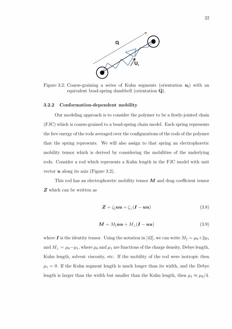
Figure 3.2: Coarse-graining a series of Kuhn segments (orientation ui) with anequivalent bead-spring dumbbell (orientation Q).

3.2.2 Conformation-dependent mobility

Our modeling approach is to consider the polymer to be a freely-jointed chain

(FJC) which is coarse-grained to a bead-spring chain model. Each spring represents

the free energy of the rods averaged over the configurations of the rods of the polymer

that the spring represents. We will also assign to that spring an electrophoretic

mobility tensor which is derived by considering the mobilities of the underlying

rods. Consider a rod which represents a Kuhn length in the FJC model with unit

vector u along its axis (Figure 3.2).

This rod has an electrophoretic mobility tensor M and drag coefficient tensor

Z which can be written as

Z = ζ‖uu+ ζ⊥(I − uu) (3.8)

M =M‖uu+M⊥(I − uu) (3.9)

where I is the identity tensor. Using the notation in [42], we can writeM‖ = µ0+2µ1

andM⊥ = µ0−µ1, where µ0 and µ1 are functions of the charge density, Debye length,

Kuhn length, solvent viscosity, etc. If the mobility of the rod were isotropic then

µ1 = 0. If the Kuhn segment length is much longer than its width, and the Debye

length is larger than the width but smaller than the Kuhn length, then µ1 ≈ µ0/4.

23

Lee and Larson have described a way of calculating the effective mobility of a FJC

from the mobility. In the notation used here, the effective mobility of the FJC is

denoted by µ and solves

〈Z〉 · µ = 〈Z ·M〉 (3.10)

where the angle brackets denote an average over the orientation distribution of the

rods. This distribution is not isotropic and is restricted by how extended the chain

is; if the chain is near equilibrium the rods will be almost isotropic while if the

chain is stretched the rods will be highly aligned. Our goal is to determine this

distribution from the extension of a spring in the coarse-grained model, calculate

the averages over u to determine the effective mobility of the spring µ, then use

that mobility in the dynamics of the spring.

Consider a spring whose extension vector is denoted as Q (Figure 3.2) and

whose maximum extension is Q0 = NkAk where Nk is the number of Kuhn steps

that the spring represents and Ak is the Kuhn length. The spring with extension Q

represents an average over all FJC configurations for which the end to end vector is

Q. Therefore the extension must be related to the average of a rod Q = NkAk〈u〉.

To simplify the notation, we will denote n ≡ 〈u〉, so that Q/Q0 = n. The stretch of

the spring determines the average of the rod orientation vector, but does not directly

determine the distribution. We follow a similar approach as Lee and Larson and

postulate that the distribution is the one in which the rod is subject to an external

“force” f , and the force is determined such that the average over the distribution is

the correct, known average. Therefore, the probability distribution of rod angles is

P (u) ∝ exp(βf (n) · u) where we have explicitly noted that the force is a function

of the average u and β = 1/(kBT ).

This choice is only self-consistent if we calculate the average angle and obtain

n. Because the distribution is well known, we can calculate the average analytically.

24

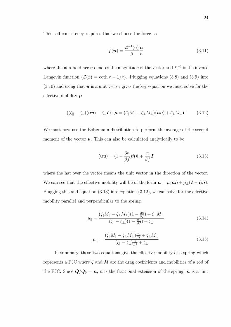
This self-consistency requires that we choose the force as

f (n) =L−1(n)

β

n

n(3.11)

where the non-boldface n denotes the magnitude of the vector and L−1 is the inverse

Langevin function (L(x) = coth x − 1/x). Plugging equations (3.8) and (3.9) into

(3.10) and using that u is a unit vector gives the key equation we must solve for the

effective mobility µ

((ζ‖ − ζ⊥)〈uu〉+ ζ⊥I) · µ = (ζ‖M‖ − ζ⊥M⊥)〈uu〉+ ζ⊥M⊥I (3.12)

We must now use the Boltzmann distribution to perform the average of the second

moment of the vector u. This can also be calculated analytically to be

〈uu〉 = (1− 3n

βf)nn+

n

βfI (3.13)

where the hat over the vector means the unit vector in the direction of the vector.

We can see that the effective mobility will be of the form µ = µ‖nn+ µ⊥(I − nn).

Plugging this and equation (3.13) into equation (3.12), we can solve for the effective

mobility parallel and perpendicular to the spring.

µ‖ =(ζ‖M‖ − ζ⊥M⊥)(1− 2n

βf) + ζ⊥M⊥

(ζ‖ − ζ⊥)(1− 2nβf) + ζ⊥

(3.14)

µ⊥ =(ζ‖M‖ − ζ⊥M⊥)

nβf

+ ζ⊥M⊥

(ζ‖ − ζ⊥)nβf

+ ζ⊥(3.15)

In summary, these two equations give the effective mobility of a spring which

represents a FJC where ζ and M are the drag coefficients and mobilities of a rod of

the FJC. Since Q/Q0 = n, n is the fractional extension of the spring, n is a unit

25

vector directed along the spring, and f is given by the self-consistency condition in

equation (3.11). It is useful to point out some important limiting cases of equations

(3.14) and (3.15). This will provide physical insight into the nature of the formulas.

The first special case is M‖ = M⊥. In this limit, the rod has an isotropic

mobility, and the formulas lead to an isotropic mobility for the spring µ‖ = µ⊥.

The second special case is ζ‖ = ζ⊥. In this limit, the drag coefficient is isotropic,

and the formulas lead to a spring mobility which is a linear combination of the rod

mobilities. If the drag coefficient is not isotropic, the spring mobility is still a linear

combination of the rod mobilities but the drag coefficients change how strongly the

rod mobilities are weighted.

The one complication using these effective mobilities in a bead-spring chain

simulation is the inverse Langevin function in equation (3.11). Computing this in-

verse for each spring at each timestep would make the method more computationally

costly. A Pade approximant has been previously developed by Cohen [80] to ap-

proximate the inverse Langevin function. Therefore we will use this approximation

βf = L−1(n) ≈ (3n− n3)/(1− n2). With this approximation, the spring mobilities

become an explicit function of n, the fractional extension of the spring, as

µ‖ =(ζ‖M‖ − ζ⊥M⊥)(

1+n2

3−n2 ) + ζ⊥M⊥

(ζ‖ − ζ⊥)(1+n2

3−n2 ) + ζ⊥(3.16)

µ⊥ =(ζ‖M‖ − ζ⊥M⊥)(

1−n2

3−n2 ) + ζ⊥M⊥

(ζ‖ − ζ⊥)(1−n2

3−n2 ) + ζ⊥(3.17)

As a last step, we generalize this dumbbell model of conformation-dependent

electrophoretic mobility over a bead-spring chain, by averaging the mobility of the

two springs adjoining a bead and assigning it as the mobility represented by that

bead. This averaging approach accounts for chain contiguity in linear polyelec-

trolytes.

26

3.3 Simulation Methodology

In this work we use the standard Brownian Dynamics (BD) simulation method-

ology [81–84]. Since BD can coarse-grain out the fast modes of the solvent, it allows

one to simulate efficiently much larger time-scales than Molecular Dynamics. BD

simulations are particularly well suited to studying the structure and rheology of

complex fluids in various nonequilibrium situations [44, 83, 85, 86].

Here, we coarse-grain our DNA molecule to a bead-spring chain, in which

the solvent and dissolved ions are treated as a continuum that give rise to viscous

drag, Brownian fluctuations, and hydrodynamic interactions. The beads (1 − Nb)

represent the hydrodynamic drag experienced by the molecule, while the springs

represent the entropic restoring force associated with stretching a sub-section of the

chain. We employ a Finitely Extensible Nonlinear Elastic (FENE) [87] spring force

model. This model is linear at small extensions but becomes nonlinear at larger

extensions to prevent the polymer from stretching beyond its finite length, and has

been verified experimentally to capture the elasticity of polymers.

We assume that the electrohydrodynamic interactions only occur between dif-

ferent parts within a rod of the FJC and not between rods. This leads to a mobility

of a spring that depends on conformation (as discussed in the previous subsection).

In the bead-spring chain model, the bead positions are tracked and they are the

points where the hydrodynamic and electric field forces are applied. The stochastic

equation for the change in the position of bead i, derived from a force balance on

the bead, is

dri =

[

u∞(ri) +

Nb∑

j=1

Pij ·E(rj) +1

kBT

Nb∑

j=1

Dij · Fj +

Nb∑

j=1

∂

∂rj·Dji

]

dt+√2dt

Nb∑

j=1

Bij ·dWj

(3.18)

where Nb is the number of beads, ri is the position of bead i, u∞ is the imposed

27

external fluid flow evaluated at the position of the bead, Pij is the effective elec-

trophoretic mobility tensor describing how fields at bead j alter the motion of bead

i, E is the external electric field evaluated at the position of bead j, Dij is the

hydrodynamic diffusion tensor, Fj is the net of spring forces and excluded volume

forces on bead j, and dWj is a vector of random variables with zero mean and

variance 1.

In order to satisfy the fluctuation-dissipation theorem [82], the tensor Bij must

obey

Dij =

Nb∑

k=1

Bik ·BTjk (3.19)

Hydrodynamic diffusion tensor in confinement

For a system of point forces acting on the fluid, the velocity v at any given

point in the fluid is the solution to the incompressible Stokes’ flow problem

µ∇2v = ∇p+∑

i

fi δ(r− ri), (3.20)

∇ · v = 0, (3.21)

with the appropriate boundary conditions. In the absence of any forces on the fluid

by the particles, the unperturbed velocity u(ri) = v(ri) at the location of a particle

i. The velocity at point i due to a point force at j can be written in a general form

as

vi = Ωij · fj , (3.22)

where Ωij is known as the hydrodynamic interaction tensor, or Green’s function.

The diffusion tensor is written using the Green’s function as

Dij =kBT

ζIδij + kBTΩij, (3.23)

28

where ζ is the drag coefficient.

In an infinite domain, the velocity perturbation due to a point force is given

by the Oseen-Burgers (OB) tensor [6, 88, 89],

Ωii = 0 (3.24)

Ωij =1

8πηrij

[

I+rijrij

r2ij

]

. (3.25)

The Green’s function for an arbitrary geometry can be expressed as

Ω = ΩOB +ΩW , (3.26)

where ΩOB is the free-space Green’s function and ΩW is the addition that accounts

for the no-slip condition at the walls of the geometry. The velocity due to a point

force acting at rj is then written as

v(r) = vOB(r− rj) + vW (r, rj)

= [ΩOB(r− rj) +ΩW (r, rj)] · fj .(3.27)

The velocity v(r) is calculated from the solution of the incompressible Stokes’

flow problem (equations (3.20) and (3.21)) along with this extra boundary condition

at the walls,

v = vOB + vW = 0. (3.28)

The Stokes flow problem can be numerically solved to calculate ΩW . The hydrody-

namic tensor in equation (3.23) can be written as

Ωij = ΩW (ri, rj) + (1− δij)ΩOB(ri − rj). (3.29)

29

A nonsymmetric diffusion tensor violates the reciprocity relation

Ω(ri, rj) = ΩT (rj, ri), (3.30)

which results from self-adjointness of the Stokes operator [90]. This can be over-

come by the following approach suggested by Jendrejack [91] and Felderhof [92] to

obtain a symmetric positive-semidefinite diffusion tensor, for |rij| ≥ 2a. The wall

correction ΩWij , which is not equal to (ΩW

ji )T , is used to construct a symmetric,

positive-semidefinite tensor by

Ωij =ΩW

ij + (ΩWji )

T

2, (3.31)

Ωji =ΩW

ji + (ΩWij )

T

2, (3.32)

where (ΩWji )

T denotes the tensor transpose of ΩWji . Ω is symmetric as we have

Ωij = ΩTji from equations (3.31) and (3.32).

Further, we discuss our approach of using Blake’s solution [93] to calculate

Wall HI in the Appendix.

Throughout most of the thesis we will utilize our new model which only in-

cludes electrohydrodynamic interactions within a rod of the FJC and not between

rods. These mean that the mobility tensor Pij is zero if i 6= j and equals µi when

i = j.

The springs in the chain have a spring force given by the FENE force relation

[87]

F =HQ

1− (Q/Q0)2(3.33)

whereQ is the extension of the spring, Q0 is the maximum spring extension, andH =

3kBT/(AkQ0). This relation, which is an approximation of the response of a freely-

30

jointed chain, is used to be consistent with the model of electrophoretic mobility

which used a freely-jointed chain. All chains in this work are chosen to approximately

represent λ-DNA which has approximately 200 Kuhn steps in the whole chain. The

beads also interact with an exclude volume potential which represents the preference

of the polymer coils represented by the springs to not be overlapping. This potential

is a soft Gaussian given by [91]

Uevij =

1

2vkBTN

2k,s

(

3

4πS2s

)3/2

exp

(−3 | rj − ri |24S2

s

)

(3.34)

where v is the excluded volume parameter, and Ss is the radius of gyration of an

ideal chain consisting of Nk,s Kuhn segments.

The strength of the fluid flow and electric field is quantified using a dimen-

sionless parameter called the Weissenberg number. The Weissenberg number is

Wi = ǫλ, where ǫ is the fluid velocity gradient and λ is the longest relaxation time

of the polymer. For Wi > 1 the fluid gradients are large enough to stretch the poly-

mer. The strength of the electric field is quantified using WiE = ǫEλ in which the

nominal electrophoretic mobility µo is used to convert electric field gradients into

an effective “velocity” gradient ǫE . In the straight channel simulations, the average

shear rate across the channel is used to obtain Wi; WiE is defined such that when

Wi =WiE , the average fluid flow velocity equals the (uniform) electrophoretic flow

velocity.

Since our polymer model includes explicit bead-bead and wall hydrodynamic

interactions, we employ the theoretical Zimm polymer relaxation time [7] for ob-

taining the Weissenberg numbers.

Our model employs explicit Euler time stepping for simulations which do not

include explicit HI between beads and uses Fixman’s mid-point time stepping algo-

rithm [94] for simulations which include HI.

31

Having developed our coarse-grained model for conformation-dependent elec-

trophoretic mobility, we ran simulations to verify that our model correctly captures

experimental observations that rely on conformation-dependent mobility of ds-DNA.

3.4 Model Verification

3.4.1 Straight channel migration

One important observation in both experiments and simulations that results

from conformation-dependent electrophoretic mobility is the migration of polyelec-

trolytes across streamlines in straight channels with both pressure-driven flow and

electric fields applied in a parallel manner. Therefore, this acts as an important

validation of our new coarse-grained model.

The results of [49] describe a mechanism for the migration. Specifically, the

pressure-driven flow will deform the polymer from its coiled and isotropic state.

This change in conformation changes the mobility. In particular, the major axis of

the radius of gyration tensor is tilted at an angle relative to the electric field which

leads to a migration velocity across the channel.

Our coarse-grained model can undergo the same mechanism but in which the

reason for the change in mobility and the way it is captured in the model are

different. In the model of [41], the beads which can be relatively far apart along the

polymer contour directly interact with electrohydrodynamic interactions. Instead,

our model only includes the interactions within a single rod of each Kuhn segment,

which gives a spring a mobility that depends on its extension and orientation.

In the simulations, a parabolic fluid velocity profile u∞ is imposed along with

a constant electric field E. The fluid flow is in the x-direction and is given by

u∞x = γH(1− (y/H)2), where γ is the average shear rate, y is the distance from the

32

Position of CM in Channel (y/H)-1 -0.8 -0.6 -0.4 -0.2 0 0.2 0.4 0.6 0.8 1

P(y

/H)

0

1

2

3

4

5

6

7

Figure 3.3: Capillary electrophoresis (rectangular channel) with pressure-drivenflow showing migration across the streamlines for co-current opera-tion (migration towards the center). The four models used are (i)explicit EHI in 5-bead chain (red,squares), (ii) new model with onespring (blue,diamonds), (iii) new model with 5-bead chain, including HI(green,circles), and (iv) new model with 10-bead chain (black,crosses).Wi = 0.9 and WiE = 1.9254.

Position of CM in Channel (y/H)-1 -0.8 -0.6 -0.4 -0.2 0 0.2 0.4 0.6 0.8 1

P(y

/H)

0

2

4

6

8

10

12

14

16

18

20

Figure 3.4: Capillary electrophoresis (rectangular channel) with pressure-driven flowshowing migration across the streamlines for counter-current opera-tion (migration towards the walls). The four models used are (i)explicit EHI in 5-bead chain (red,squares), (ii) new model with onespring (blue,diamonds), (iii) new model with 5-bead chain, including HI(green,circles), and (iv) new model with 10-bead chain (black,crosses).Wi = 0.9 and WiE = −1.9254.

33

center of the channel, and H is the half height of the channel. The strength of the

fluid flow is quantified by a Weissenberg number as Wi = γτ where τ is the longest

Rouse relaxation time given by τ = ζ/(8H sin2(π/(2Nb))).

The electric field points parallel to the x-direction, is uniform across the chan-

nel, and with strength quantified by an electric Weissenberg number WiE . Because

the electric field is uniform, this is not defined using a gradient of the electric field.

Instead, it is defined such that WiE = Wi corresponds to the condition when µ0E

equals the mean fluid flow. With this definition, WiE = 3µ0Eτ/(2L). The experi-

ments and simulations correspond to Wi = 0.9 and WiE = ±1.9254.

We have simulated a dumbbell, 5-bead chain and 10-bead chain polymer mod-

els in the straight channels. In addition to simulating with our new coarse-grained

mobility model, we also did simulations with the older model of [41] to verify our

model. The polymer simulations represent an average of 50 trajectories, with initial

conformations for each obtained from long-time decorrelated runs. Each trajectory

is run for 20 wall diffusion times, which captures sufficient data across the channel

width for each trajectory.

Figures 3.3 and 3.4 show the straight channel migration results for our model.

We plot the normalized probability distribution of the polymer’s center-of-mass

versus the position of its center-of-mass across the channel width. The four models

shown are: (i) Butler’s Explicit EHI model in 5-bead chain (red,squares), (ii) new

model with one spring (blue,diamonds), (iii) new model with 5-bead chain, including

HI (green,circles), and (iv) new model with 10-bead chain (black,crosses).

Comparing the Butler’s model (old) with our model, we see that our new model

captures both co-current and counter-current migration accurately when compared

to a previous simulation [41] and experiments [49]. We also see that the number of

beads in the model has a weak effect on the migration, which shows that around

34

5−10 beads are sufficient to capture migration while also achieving a high simulation

efficiency.

The results in this section validate the new model in situations in which the

polymer is weakly deformed from equilibrium and show that the model can capture

migration perpendicular to the electric field. However, one of the main advantages

of the new model is that it can also easily capture the response when the molecule is

highly stretched such as in extensional electric field gradients, which are examined

in the next section.

3.4.2 Stretching in an electric field gradient

Electric field gradients have been used extensively to stretch DNA in microflu-

idic devices. In electrostatics, the electric field has zero curl which can facilitate large

stretching of the DNA. Experimentally it has been observed that DNA molecules

have different mobilities when stretched [42]. When a molecule is stretched in

a strong extensional field, a number of folded and kinked configurations are ob-

served [10, 44]. The work of Larson and coworkers [42] showed that these folds and

kinks can lead to configurations that have the same visual length but a different

mobility. They developed a 1-D model that explained this phenomena by writing

the mobility in terms of the average alignment of a Kuhn segment. In this section,

we show simulations of our 3-D model in extensional field gradients. The dynamics

of the molecules will lead to a variety of configurations including kinks and folds.

In the simulations we impose a planar extensional field given by Ex = ǫEx,

Ey = −ǫEy, Ez = 0 without an external fluid flow. The electric field gradients are

quantified by a Weissenberg number WiE defined by WiE = µ0ǫEτ which uses the

nominal mobility µ0. Note that this definition is different from the one used in the

straight channels in the previous section. Simulations are performed using a polymer

model made of 20 beads (19 springs) so that kinked and folded configurations can

35

0 1 2 3 4 50

0.1

0.2

0.3

0.4

0.5

0.6

0.7

0.8

0.9

1

Hencky Strain Units

Vis

ual (

Str

etch

) Le

ngth

(X

/L)

Figure 3.5: Scatter plot of the chain stretch as a function of the Hencky strain.WiE = 90 for a total of 5 Hencky strain units. The different symbolsrepresent different molecules.

be observed [44].

We performed simulations with our new model at WiE = 3, 30 and 90, for a

total of 5 Hencky strain units each, using a 20 bead-spring chain. For these condi-

tions, the polymer stretches significantly, which allows us to test our model for large

deformations. For each WiE , we ran 50 independent trajectories, with decorrelated

starting configurations for the trajectories obtained from long-time equilibrium (no-

field) runs.

Figure 3.5 shows the time dynamics of stretching of the DNA molecules. We

find that the stretching rate can vary widely based on the initial conformation of

the molecules at the start of extension, which is termed as ‘Molecular Individualism’

[43, 44].

36

Visual (Stretch) Length (X/L)0 0.2 0.4 0.6 0.8

µE/µ

E o

0.9

1

1.1

1.2

1.3

1.4

1.5

Figure 3.6: Scatter plot of the electrophoretic mobility of ds-DNA as a function ofthe chain stretch. WiE = 3 for a total of 5 Hencky strain units. Thedifferent colors/symbols represent different molecules.

Visual (Stretch) Length (X/L)0 0.2 0.4 0.6 0.8 1

µE/µ

E o

0.9

1

1.1

1.2

1.3

1.4

1.5

Figure 3.7: Scatter plot of the electrophoretic mobility of ds-DNA as a function ofthe chain stretch. WiE = 30 for a total of 5 Hencky strain units. Thedifferent colors represent different molecules.

37

0 0.2 0.4 0.6 0.8 10.9

1

1.1

1.2

1.3

1.4

1.5

Visual (Stretch) Length (X/L)

µE/µ

E o

Figure 3.8: Scatter plot of the electrophoretic mobility of ds-DNA as a function ofthe chain stretch. WiE = 90 for a total of 5 Hencky strain units. Thedifferent symbols represent different molecules.

Figures 3.6, 3.7 and 3.8 represent the dynamics of ds-DNA molecules which

stretch in a planar extensional electric field with a WiE = 3, 30, 90 respectively for

a total of 5 Hencky strain units each. The electrophoretic mobilities were obtained

from the instantaneous center-of-mass velocities of the polymer, divided by the

electric field at that position.

The key feature of these plots are that the electrophoretic mobility increases

with increasing stretch, similar to experiments [42]. For lower WiE they all basi-

cally fall on the same curve which is how the stretch of a spring behaves because

there are no significant kinks or folds formed, leading all configurations to stretch

quantitatively similarly.

But for larger WiE there are a variety of curves leading to multiple mobilities

at the same stretch. This, in conjunction with Figure 3.5, shows that the stretching

38

mode and the rate of stretching can vary widely based on the initial conformation

of the molecules at the start of the stretch. Two molecules can have the same

stretch but different mobility. This results from the formation of folds and kinks

in the polymer chain, which can give a high electrophoretic mobility even at low

to moderate visual stretch. Kink dynamics has been analyzed previously using

simulations [44].

3.5 Conclusions

Polyelectrolytes that are deformed in fluid flows and electric fields change

their electrophoretic mobility depending on their conformation. This change is

due to electrohydrodynamic interactions between parts of the polymer. There are

some similarities but key differences with how hydrodynamic interactions lead to

conformation-dependent drag. The changes in mobility occur for even relatively

short polymers, and are approximately a local effect along the polymer backbone

when its is strongly stretched from equilibrium.

In this chapter, we have developed a new coarse-grained model that can be

used for dynamical simulations of polymers like ds-DNA in combinations of fluid

flows and electric fields. The model assigns an electrophoretic mobility tensor to

each bead that is a function of the stretch and orientation of the springs that are

connected to the bead.

The model has been validated in two situations: combined electrophoresis and

pressure-driven flow in a channel with the polymer weakly deformed from equilib-

rium and planar extensional electric field gradients that stretch the polymer far

from equilibrium. In capillary electrophoresis the model captures the cross-stream

migration due to stretching of the chain at an angle to the electric field. In strong

extensional fields the model captures the folded and kinked configurations that have

39

a large impact on the mobility of the chain.

For large electric fields, the model shows the chain can unravel these folds in a

way not seen previously in simulations or experiments. The unique unfolding is due

to the fact that the dynamics are dependent on the location of the center of mass

of the chain even though the electric field gradients are uniform in the system.

This coarse-grained model will allow for rapid simulations in situations with

combinations of electric fields and fluid flows, for example in the trapping and ma-

nipulation of molecules in microfluidic devices which will be shown subsequently.

4. SIMULATIONS OF TRAPPING AND

MANIPULATION OF DEFORMABLE OBJECTS

Having developed a new coarse-grained model of conformation-dependent elec-

trophoretic mobility, elaborated in the previous chapter, we are motivated to apply

the model to simulate both flexible as well as rigid orientable objects with the goal

of either trapping them or manipulating them in different ways.

In this chapter, we discuss simulations of flexible polymers, in both confined

microfluidic geometries as well as infinite elongational fluid flows and electric fields.

An advantage of directly simulating these microfluidic geometries is that we can

perform microfluidic experiments with analogous conditions with an aim to replicate

simulation findings. Simulations of trapping and manipulation of rigid rods will be

elaborated in the next chapter.

4.1 Trapping Objects in Confined Microfluidic Geometries

We have performed simulations using the new Brownian dynamics model of a

deformable polymer molecule in both T- and Cross channels with pressure-driven

flow and electric field gradients applied. The fluid flow velocity and the electric field

is solved once for each microfluidic geometry using ABAQUS software that uses a

Finite Element method to solve Laplace’s equation for the electric potential (and

electric field) and the Navier-Stokes equation for the fluid flow.

For the fluid flow, we have the Navier-Stokes and Continuity equations:

ρ(∂t + v · ∇)v = −∇p + µ2v and (4.1)

40

41

∇ · v = 0 on Ω (4.2)

With a no-slip velocity boundary condition at the wall,

v|wall = 0 on ∂Ω (4.3)

where ρ is the fluid density, v is the fluid velocity, p is the hydrodynamic pressure,

µ is the fluid viscosity, Ω is the fluid domain and ∂Ω represents the fluid boundary.

For the electric potential, we have Laplace’s equation:

∇2Φ = 0 on Ω (4.4)

With either a specified potential boundary condition (at the electrodes) or an

insulating boundary condition (at PDMS or glass surface).

Φ = Φ|given or∂Φ

∂n= 0 on ∂Ω (4.5)

With the electric field defined as E = −∇Φ

where Ω is the fluid domain and ∂Ω represents the fluid boundary.

A cubic mesh is used for the FEM, with a mesh size ∼ the radius of gyration

of the polymer chain. Mesh size independence in our FEM results is verified by

running a finer mesh and comparing the result with the coarser mesh. A look-up

table is made for the velocity and electric field at each discretized point in the

domain, which is linearly interpolated during the course of the BD simulation.

Similar to Chapter 3, we represent the 21µm λ−DNA as a bead-spring chain,

42

Figure 4.1: Simulation of a polymer in a T-channel with Wi = 2 and WiE = −3.96.The green arrows show the effective field seen by a molecule withoutconformation-dependent mobility. The curves show the trajectories ofthe polymers in the simulation with the molecules beginning at thecenter of the channel (X = 0, Y = 0). The red curve shows that amolecule with constant mobility recirculates many times before a Brow-nian fluctuation allows it to leave. The blue curve shows a molecule withconformation-dependent electrophoretic mobility. When the moleculestretches, the mobility changes, which leads to an unbalance that pushesthe molecule away from the T-junction.

and use a 5-bead and a 10-bead model. In this confined microfluidic system, bead

confinement with respect to the boundaries is enforced with a Heyes-Melrose al-

gorithm [95]. Wi is the flow Weissenberg number and WiE is the electrophoretic

Weissenberg number.

One important observation is that molecules can be trapped based on whether

conformation-dependent mobility is important. In particular, we show that for a par-

ticular choice of E and v, a molecule without varying mobility will be trapped while

a molecule that changes its mobility when deformed will pass through the device.

43

Figure 4.2: Combined flow and field streamlines in a Cross channel with Wi = 2and WiE = −3.96. The blue arrows show the effective field seen by amolecule without conformation-dependent mobility.

Figure 4.1 shows the results of these simulations with Wi = 2 and WiE = −3.96.

The molecule without conformation-dependent mobility is trapped in a recircula-

tion region of the streamlines. In contrast, when the molecule with conformation-

dependent mobility stretches in the T, the mobility increases, which makes the E

field contribution dominate. This electric field pushes the molecule rapidly through

the T. Figure 4.2 shows the combined flow and field streamlines in a Cross channel

with Wi = 2 and WiE = −3.96. The symmetry in the Cross channel leads to

the formation of four recirculations in the effective field streamlines, which can be

similarly used to trap objects.

The mechanism for these dynamics is important and interesting because it

relies on a coupling between the dynamics of the molecule and the effective field

causing those dynamics; the deformability of a molecule alters the effective field

that it sees and how that field pushes the molecule through the device and deforms

it. An important feature to the dynamics seen here is that even when Wi and WiE

are similar in magnitude, the effective fields do not exactly cancel. This is what leads

44

to the recirculation region that traps the molecule without conformation-dependent

mobility.

The difference in fields results from a difference in boundary conditions for

the electric field and the fluid velocity. The fluid flow must satisfy no slip and

no penetration on all solid surfaces, while the electric field must only have zero

normal component (because glass and PDMS are effectively insulating compared

to the electrolytic solution). If the channel is very thin, the fluid flow will be a

“Hele-Shaw” flow. This flow is locally parabolic in the thin direction with the

mean of the parabolic flow solving the same equation as the electric field. However,

the side walls will impart different boundary conditions. In Figure 4.1, it is the

boundary conditions at the side walls that produce the recirculation regions. From

the simulation, the difference in the elution times for the two species is ∼ 33 polymer

relaxation times, equivalent to ∼ 10s, which is significant and easily observable

experimentally using modern detection methods.

4.2 Manipulating Objects in Unconfined Flows and Fields

In addition to trapping and separating objects based on their deformability,

it is useful to be able to manipulate and deform objects. In this way, we can hold

an object in one place and measure how it responds to external manipulation. This

has been done previously using fluid flows or electric fields, as described earlier in

the Background (Ch.2). Those methods rely on a control scheme to trap an object.

In order to stretch an object, large electric fields or fluid flows must be used. These

will also give rise to relatively high velocities through the device (short residence

times) that must be compensated by the control scheme. One advantage of using a

combination of electric fields and fluid flow is that conformation-dependent mobility

leads to new ways to manipulate the stretch and residence time.

45

Figure 4.3: Simulation of a polymer in an ideal combination of an elongational elec-tric field and fluid flow. All data are for simulations withWi+WiE = 10.This produces a large stretch and short residence time without EHI.With EHI we can manipulate the stretch while keeping long residencetimes. Position of the center of mass as a function of time forWi = 83.33(black), Wi = 120 (green), and Wi = 187.5 (red). For comparison, weshow the center of mass motion for a molecule without conformation-dependent mobility (blue). L is the stretched length of the dumbbelland λ is the longest relaxation time of the dumbbell.

This is shown explicitly in Figures 4.3 and 4.4, in which we show the results

from BD simulations. In these simulations, the molecule is placed at the stagnation

point in a combination of a pure planar elongational electric field gradient and a

pure elongational fluid flow gradient. The data shows a plot of the position of the

molecule center versus time as well as the stretch of the dumbbell model. The stretch

reaches a steady state while the center of mass moves away from the stagnation

point exponentially, just as in conventional elongational fields. However, the key

feature is that by manipulating the Wi and WiE , we produced cases with different

stretches with much longer residence times than those which would be experienced

by a molecule with constant electrophoretic mobility.

Mathematically, we can understand the response using a dumbbell polymer

46

Figure 4.4: Simulation of a polymer in an ideal combination of an elongational elec-tric field and fluid flow. All data are for simulations withWi+WiE = 10.This produces a large stretch and short residence time without EHI.With EHI we can manipulate the stretch while keeping long residencetimes.The corresponding stretch of the molecules as a function of timefor Wi = 83.33 (black), Wi = 120 (green), and Wi = 187.5 (red). Lis the stretched length of the dumbbell and λ is the longest relaxationtime of the dumbbell.

Figure 4.5: Polymer dumbbell in a combination of elongational electric field andfluid flow. The fluid flow Wi is countered by the electrophoretic WiE ,with their sum (Wi+WiE) depicted by the arrows. The polymer dumb-bell has a stretch Q.

47

model (Figure 4.5) and writing the equations that quantify the dynamics of the

center of mass and the vector Q connecting the two beads. For large Wi and WiE ,

Brownian forces will be small compared to the flow and field induced forces, and

the velocity of the center of mass is

drcmdt

= v|cm + µEPspr · E|cm (4.6)

where the fluid velocity and electric field are evaluated at the center of mass. The

dynamics of the vector Q is related to the gradients of the flow and field across the

polymer and is given by

dQ

dt= Q · ∇v + µEP

spr · (Q · ∇E)− 2FC

ζ(4.7)

where FC is the FENE spring connector force. For a pure extensional fluid flow and

electric field gradient, we can simplify these equations. In addition, if (Wi+WiE) >

1, the polymer will be strongly aligned along the flow’s extensional axis (the x

direction) so we only need to write the dynamics in the x direction. These simplified

equations are

dxcmdt

=xcmλ

(

Wi+WiE +4

3

(

µ1

µ0

)

f 2

1− f 2/3WiE

)

(4.8)

dQx

dt=Qx

λ

(

Wi+WiE +4

3

(

µ1

µ0

)

f 2

1− f 2/3WiE − 1

2(1− f 2)

)

(4.9)

where we have used the FENE connector spring force. f is the fractional extension

of the dumbbell and λ is the longest relaxation time of the dumbbell.

The results in Figures 4.3 and 4.4 can be understood using these equations.

48

Trajectory Number0 10 20 30 40 50 60 70 80 90 100

t /λ

0

1

2

3

4

5

Figure 4.6: Plot of the residence time (scaled by the relaxation time) versus tra-jectory number for a polymer with conformation-dependent mobil-ity (dashed), polymer without conformation-dependent mobility (dot-dashed) and a rigid sphere having the same hydrodynamic drag and elec-trophoretic mobility as the polymer (solid). Wi = 12.24,W i+WiE = 2.The dot-dashed and the solid lines overlap.

The fractional extension f is determined from Equation (4.9) by requiring that Qx

does not change in time. In this way, both Wi and WiE will affect the stretch of

the molecule. This value of f can then be placed into Equation (4.8) to determine

the rate at which the molecule leaves the device. Note that the equations have all

terms in common except the spring force 1/(2(1 − f 2)), which diverges when the

molecule is fully extended. The common terms and the sign of the spring force

leads to center of mass dynamics in Equation (4.8) corresponding to molecules that

leave the device. This is only true for deformable objects. When we examine rigid,

orientable objects in Ch.5, we will show trapping of objects without active control.

Additionally, we performed simulations in infinite flow and field (Wi = 12.24,W i+

WiE = 2) with rigid spheres, having the same hydrodynamic drag and electrophoretic

mobility as the polymer, thus serving as controls. Figure 4.6 shows the result of the

simulation. We note that the polymer with conformation-dependent mobility elutes

slowly. The polymer without conformation-dependent mobility is very similar to

49

the rigid sphere in elution time, since both are effectively only acted upon by the

net Wi+WiE = 2. Also, we note that since the flow and fields are strong compared

to Brownian diffusion, the elution times are pretty deterministic between different

simulation runs for all the models.

4.3 Conclusions

In this chapter we have discussed simulations of flexible polymers, in both

confined microfluidic geometries as well as infinite elongational fluid flow and electric

fields. An advantage of directly simulating these microfluidic geometries is that we

can perform microfluidic experiments with analogous conditions with an aim to

replicate simulation findings.

We have shown that in the confined microfluidic geometries, the difference in

the boundary conditions for the fluid flow and the electric field leads to interesting

combined flow streamlines, with recirculating patterns which can trap objects. Of

course, the deformability of a molecule alters the effective field that it sees and how

that field pushes the molecule through the device and deforms it.

In unconfined flows and fields, we have shown through theory and simulations

that conformation-dependent mobility leads to new ways to trap objects as well as

to manipulate the stretch of trapped objects.

5. SIMULATIONS OF TRAPPING AND

MANIPULATION OF RIGID ORIENTABLE OBJECTS

5.1 Introduction

It is important for many applications to be able to manipulate and separate ob-

jects with electrophoretic mobilities that depend on conformation, such as ds-DNA.

Moreover, the mobility can also depend on conformation for a rigid object provided

that the object is nonspherical and orientable. For example, a long slender rigid rod

will have a different mobility depending on the orientation of the rod relative to the

electric field. This orientation can be altered by the fluid flow gradients and electric

field gradients in the devices described here. Therefore, we expect similar principles

developed for polymers to apply to rigid rods. The goal of this work is to test that

hypothesis using computer simulations. An undergraduate student from the CBE

department, Sylvia Szafran, has collaborated on this research.

5.2 Rigid Rod Model

Two important systems of rigid rods that can be manipulated using the tech-

niques in this work are rod-like viruses and carbon nanotubes. Tobacco Mosaic Virus

(TMV) is monodisperse, and has been used by many researchers including for bind-

ing, deposition, and assembly of a variety of inorganic and organic materials [96,97]

and in nanomedicine for the design of nanocontainers and nanovaccines [98]. TMV

has a width of 18nm and a length of approximately 300nm, and is charged due to the

proteins that make up the capsid [99]. The fluorescent probe Cy3-succinimidyl ester

can be attached to the surface for visualization in video fluorescence microscopy.

The diffraction of light limits the ability to resolve the orientation of TMV, but

50

51

the center of mass can still be tracked. The relevant timescale of reorientation due

to Brownian motion is related to the rotational diffusivity as λ = 1/(6Dr). The

rotational diffusivity for TMV has been measured to be 320s−1 [100]. The fluid

flows and electric field gradients used here will be sufficient to align the TMV and

the corresponding changes in electrophoretic mobility will allow for separation. Our

bead-spring dumbbell model, elaborated below, can be used to represent rigid rods

in general, and therefore can be applied to TMV in particular while comparing with

TMV trapping experiments in the future.

We represent the rigid rods as a 2 bead dumbbell, with the difference from

flexible polymers being that the beads in the rigid rod are connected with stiff

Fraenkel springs [101]. The rods are simulated in combination of an ideal elongation

fluid flow and electric field. As in the previous chapter, we define the Weissenberg

numbers Wi and WiE to denote the strength of the fluid flow and the electric field

respectively. In our simulations, the length scale is set to be the length of the rod,

while the time is scaled by the rotational relaxation time of the rod.

Mathematically, we can understand the response of the rigid rods using the

dumbbell model (Figure 4.5) and writing the equations that quantify the dynamics

of the center of mass and the vector Q connecting the two beads. For large Wi and

WiE , Brownian forces will be small compared to the flow and field induced forces,

and the velocity of the center of mass is

drcmdt

= v|cm + µEPspr · E|cm (5.1)

where the fluid velocity and electric field are evaluated at the center of mass. The

dynamics of the vector Q is related to the gradients of the flow and field across the

rod and is given by

52

dQ

dt= Q · ∇v + µEP

spr · (Q · ∇E)− 2FC

ζ(5.2)

where FC is the Fraenkel spring connector force. For a pure extensional fluid flow and

electric field gradient, we can simplify these equations. In addition, if (Wi+WiE) >

1, the rod will be strongly aligned along the flow’s extensional axis (the Z direction)

so we only need to write the dynamics in the Z direction. Applying Equations (5.1)

and (5.2) to a rod and replacing the spring force with a rigid constraint force Fr

leads to

dzcmdt

=zcmλ

(

Wi+WiE + 2

(

µ1

µ0

)

WiE)

(5.3)

dQz

dt=Qz

λ

(

Wi+WiE + 2

(

µ1

µ0

)

WiE − Fr

)

= 0 (5.4)

where the quantity Fr takes on whatever value necessary to keep the rod from

deforming (i.e. dQz

dt= 0). We see from equation (5.4) that conditions exist for which

Fr < 0 and the rigid rod (virus) will be pushed to the stagnation point without

active control.

5.3 Stable Trapping Using Electric and Flow Fields

Using equations (5.3) and (5.4) with Fr being the constraining force for a

Fraenkel spring gives us the range of Wi and WiE where the rod will be trapped.

Figures 5.1, 5.2 and 5.3 show a representative trapped circumstance, with Wi = 10

and WiE = −9.

In Figure 5.1, we show the center of mass components of the rod versus time.

Here the time has been nondimensionalized by the rotational relaxation time of the

rod. We see that the rod is trapped stably along all axes.

53

t / λ0 5 10 15 20 25 30 35 40 45 50

(Cen

ter

of M

ass)

/L

10-5

10-4

10-3

10-2

10-1

100

zyx

Figure 5.1: Trapping of a rigid rod in an elongational flow and field. Center of masscomponents of the rod versus time, nondimensionalized by the rotationalrelaxation time of the rod. Wi = 10, WiE = −9.

In Figure 5.2, we show the rod orientation components versus time. We see

that the rod is almost completely aligned along the Z-direction, which is the along

the flow’s extensional axis.

In Figure 5.3, we quantify the strength of the rod trapping by analyzing the

histogram of the fluctuations in the components of the rod center-of-mass.

54

t / λ0 5 10 15 20 25 30 35 40 45 50

Orie

ntat

ion/

L

-1

-0.5

0

0.5

1zyx

Figure 5.2: Trapping of a rigid rod in an elongational flow and field. Rod orien-tation components versus time, nondimensionalized by the rotationalrelaxation time of the rod. Wi = 10, WiE = −9.

-0.4 -0.3 -0.2 -0.1 0 0.1 0.2 0.3 0.4

Cou

nts

0

200

400z-center of mass

-0.6 -0.4 -0.2 0 0.2 0.4 0.6

Cou

nts

0

200

400y-center of mass

-0.6 -0.4 -0.2 0 0.2 0.4 0.6

Cou

nts

0

200

400x-center of mass

Figure 5.3: Trapping of a rigid rod in an elongational flow and field. Histogram ofthe fluctuations in the components of the rod center-of-mass. Wi = 10,WiE = −9.

55

5.4 Conclusions

In this chapter we have discussed simulations of rigid rods, in infinite elonga-

tional fluid flow and electric fields.

In these unconfined flows and fields, we have shown through theory and sim-

ulations that conformation-dependent mobility leads to new ways to trap and ma-

nipulate rigid objects. An important advantage of our trapping approach over the

previous experimental work (Ch.2, Background) is that we are able to stably and

passively trap objects along all directions, without requiring any active control of

either the fluid flows or electric fields.

6. MICROFLUIDICS EXPERIMENTS

In this chapter we describe our experiments using ds-DNA and Polystyrene

microspheres in different microfluidic geometries. Firstly, we briefly describe our

experimental setup, in terms of channel preparation, microscopy, imaging and data

analysis. Then we proceed to discuss salient observations from these experiments.

6.1 Channel Preparation

We employ Soft Lithography [102–104] to create custom microfluidic channels.

Briefly, we use a CAD program (CleWin) to design our channels, which are then

Figure 6.1: Schematic illustration of ‘Replica Molding’ : the procedure for castingPDMS replicas from a master having relief structures on its surface.Reproduced with permission from [102].

56

57

printed with high resolution on a transparency. This serves as a mask for transfer-

ring our patterns to a Si wafer using Photolithography. We spin-coat Shipley 1813

positive tone photo-resist onto Pirahna-cleaned 100-oriented Silicon wafers using a

Headway spin coater. Photolithography is then performed using a Karl Suss MJB-3

aligner. We then carry out Deep Reactive Ion Etching (DRIE) using the Alcatel

ICP DRIE equipment. Finally, we measure our channel profile using a Veeco Dektak

8 profilometer.

We then ‘Replica Mold’ [102,103] our microfluidic channels from poly(dimethylsiloxane)

(PDMS), with the etched Si wafer as the mold (Figure 6.1). Replica molding has

several advantages over conventional photolithography to prepare microfluidic chan-

nels, namely that it can generate 3-D and non-planar surfaces, and it can support

a broad range of materials, including a variety of biomaterials [102]. In general,

soft lithography has been found to be well suited for rapid and easy prototyping of

designs [102, 105], with PDMS preferred for robustness and bio-compatibility.

The PDMS device and a glass coverslip (No. 1, 24 × 60 mm) are treated

with an O2 plasma (PDC-32G, Harrick Scientific) and bonded together, creating

channels with the bottom made of glass and the top and sides made of PDMS. Our

channels typically have an arm length of 0.8cm and a cross-section of width 50µm

and depth ranging from 2.5µm to 25µm. Holes are bored in the PDMS to provide

fluidic connections at the channel arms. These range from a diameter of 4.22mm

bored by a Harris micro punch to 27gage (0.41mm) bored by Luer stubs (27 gage,

Instech Laboratories Inc).

We use Hamilton Gastight syringes ranging in volumes from 0.5µL to 500µL,

connected to the PDMS channel via Polyethylene tubing (PE-20, Instech Labora-

tories Inc). Stainless steel stubs (SS-304, 25 gage; McMaster Carr) are inserted

into the PDMS channels and act both as fluidic connectors and electrodes. Syringe

58

pumps (Fusion 400, Chemyx) and voltage generators (Model 677B, Trek) are used to

drive low Reynolds number flows [33] and electric fields in the channels. Ultrapure

water for our experiments is obtained from a Seimens Labostar ultrapure water sys-

tem. We use diluted Tris-Borate-EDTA (TBE) (Sigma Aldrich) as the electrolytic

buffer for suspending both microspheres and λ-DNA. The TBE buffer was purified

by syringing with a 0.2µm syringe filter (Acrodisc, Pall Corporation).

6.2 Microscopy, Imaging and Data Analysis

Experiments using the microfluidic devices are visualized on an inverted epi-

fluorescence microscope (Zeiss AxioObserver Z1) as shown in Figure 6.2(a). We use

40X air objectives and the 63X and 100X oil-immersion objectives. We calibrate

our objectives with a standard glass calibration slide for all our cameras to convert

lengths in pixels in the microscopic image into physical lengths (in µm). Movies

are taken of the motion of fluorescently- labeled objects that can be analyzed to

quantify the positions, velocities, and stretch of objects. Fluorescent microspheres

are used as controls as objects that cannot deform and change their mobility. Figure

6.2(b) shows a snapshot of microspheres in flow in a T-channel. Because of the large

Figure 6.2: Illustration of some of the experimental methods used. (a) PDMS mi-crochannel on an inverted epi-fluorescence microscope. (b) Image of0.5µm fluorescent microspheres in flow in a T-shaped microchannel.Dashed lines illustrate the positions of the channel walls. (c) Zoomed-inimages of dyed λ-DNA in a coiled configuration (top) and a stretchedconfiguration in a fluid flow (bottom).

59

fluorescent intensity, they can be imaged on high speed sCMOS cameras (Andor Zyla

camera, Zeiss AxioCam MRm camera and Moticam 2300 camera). λ-DNA (Nippon

Gene Co, Japan) is dyed with TOTO-1 (Invitrogen) [9–12] which intercalates into

the double helix. Because of the lower fluorescence, it necessitates the use of an

Electron Multiplying Charge Coupled Device (EMCCD) camera (Andor IXon3),

capable of single-photon capture, to record movies of the molecules.

Figure 6.2(c) shows an example image of λ-DNA both at equilibrium (in a

coil) and stretched by an external fluid flow. In the technique of video fluorescence

microscopy, each image of a movie is processed to determine the position and size

of each object using tracking codes [106, 107] written in an image analysis soft-

ware called Interactive Data Language (IDL). Briefly, the steps involved in particle

tracking include:

• Noise reduction in the images.

• Locating objects of interest.

• Refining location estimates and particle discrimination.

• Linking particle locations into trajectories.

The movement of an object from one frame to the next frame can then be

used to calculate the velocity of the object, which, coupled with its instantaneous

conformation, gives complete insight into its dynamics.

6.3 Observations At Equilibrium

Tracking Polystyrene microspheres at equilibrium

To verify our microscopy setup and our particle tracking codes, we track neu-

trally buoyant Polystyrene microspheres at equilibrium (no flow) in sealed microscope-

coverslip-wax chambers and in our PDMS channels.

60

Figure 6.3: Plot of mean-squared displacement as a function of lag time for 1µmdiameter carboxylated Polystyrene microspheres visualized at equilib-rium. Theory lines (Red) indicate Brownian diffusion. (a) Microspheresdiluted 1000-fold in 83.34% glycerol (by volume) (viscosity= 64.2cP ) inultrapure water, imaged in a coverslip-wax chamber. (b) Microspheresdiluted 1000-fold in ultrapure water, imaged in a straight PDMS chan-nel.

Figure 6.3 shows the Mean-Squared Displacement (MSD) as a function of lag

time for 1µm diameter carboxylated Polystyrene microspheres visualized at equilib-

rium. The MSD is non-dimensionalized by R2, and the lag time by a self-diffusion

timescale ζR2/KT , where R is the radius of the microsphere, ζ is the hydrodynamic

drag coefficient for the microsphere (obtained from Stokes’ law at low Reynolds num-

bers), K is the Boltzmann constant and T is the absolute temperature.

The error bars for the experimental curves represent statistical error, which is

calculated through block averaging [108]. Theory lines are simultaneously plotted

for both figures and are seen to have a good fit with the experimental data.

6.4 Observations under Fluid Flow

After having verified our microscopy and particle tracking codes through ob-

servations at equilibrium, we performed experiments of visualizing Polystyrene mi-

61

crospheres and ds-DNA in Straight and T-channels with fluid flows of varying flow

rates applied using the Syringe pump.

Figure 6.4 shows the fluid flow streaklines of 0.5µm diameter Carboxylated

Polystyrene microspheres flowing in the T-channel with an applied flow rate of

Q = 0.005µL/min from the top arm controlled through the syringe pump. The

streakline composite image is produced by summing over all the individual frames

of the fluid flow movie. The exposure time for recording the frames is 0.05s.

We then compared the experimentally observed microsphere flow velocities in

the channel inlet arm with theoretical flow velocities calculated from the externally

applied flow rate. We also have the exact velocity field for the T-channel calculated

through ABAQUS FEM, and can compare our experiments with that. Since the

velocity field is non-uniform across the channel cross-section, we make 10 bins across

the cross-section, and track an equal number of microspheres in each bin to get an

accurate velocity profile.

Against a theoretically calculated mean velocity of 66.67µm/s, the experimen-

tal mean velocity equals 61.34µm/s. Further, the experimental velocity profile, in

terms of the ratio Vmax/Vavg, was compared with that computed through ABAQUS

FEM. Against a theoretically computed Vmax/Vavg = 1.91 from ABAQUS, the ex-

periments showed a bit different velocity profile with a Vmax/Vavg = 1.71.

62

Figure 6.4: Streaklines of 0.5µm diameter carboxylated Polystyrene microspheres influid flow in a T-channel. Flow rate Q = 0.005µL/min. 1000X dilutedparticles in ultrapure water observed under a 40X objective.

6.5 Observations under Electric Field

Electro-Osmotic flow

Electro-osmotic flow, which is generated when an electric field is applied across

a channel with charged walls, is present in our devices. This is because the surfaces

used in the microfluidic devices in this work, i.e. glass and PDMS, carry a negative

charge in TBE buffers (pH ∼ 8) from dissociation of -Si(OH)3. The negative surface

charge causes the positive ions in the buffer to accumulate at the surface (in the

O[nm] Debye layer) so that there is a local imbalance of charge in the fluid near

the wall surface. The excess charge in the Debye layer will be positive for PDMS

or glass, so electro-osmotic flow would be towards the negative electrode when an

electric field is applied. Because the fluid is contained by charged walls on all sides,

the fluid moving at the walls drags the remaining fluid in the bulk of the channel.

Under the small Debye layer limit (Smoluchowski limit), a/λD ≫ 1 (a being a

characteristic length scale of the wall), and with the electro-osmotic flow velocity

63

given by

v ≈ φζǫdeE

η= µEOFE (6.1)

where φζ is the zeta potential of the surface, ǫde is the fluid permittivity, η is the

fluid viscosity, E is the electric field and µEOF is the electro-osmotic mobility of

the system. In a straight-walled channel, the induced electro-osmotic flow has a

plug profile outside the O[nm] Debye layer at the surface. Typical electro-osmotic

mobilities for 1cP fluids having a high ionic strength (O[0.1M]) is µEOF ∼ 2.5

(µm/s)/(V/cm) for PDMS and µEOF ∼ 5 (µm/s)/(V/cm) for glass [109].

These high ionic strength electro-osmotic mobilities are greater than DNA’s

electrophoretic mobility (µEP ∼ −1.3 (µm/s)/(V/cm)), so if electro-osmotic flows

are not reduced, the negatively-charged DNA will move in the opposite direction

towards the negative electrode.

We follow [109] in using a dynamic coating of Polyvinylpyrrolidone (PVP), a

non-ionic polymer which coats the channel walls upto a thickness ≫ the Debye layer

thickness. This increases the local viscosity in the fluid around the Debye layer, thus

slowing down the electro-osmotic flow. We use PVP of 104 g/mol molecular weight

(Sigma Aldrich), which has been found to be small enough to not significantly alter

DNA conformation during electrophoresis, and large enough to significantly quench

electro-osmotic flow [109, 110].

Electrophoresis of Polystyrene microspheres in straight channel

We have tracked 0.5µm diameter negatively charged (Carboxylated) and neu-

tral Polystyrene microspheres in our straight PDMS channel, with variable electric

potentials applied at the two arms. We initially tracked neutral Polystyrene micro-

spheres under the applied electric field. In this case, we expect electrophoretic flows

64

to be absent, and electro-osmotic flows to dominate. We also tracked Carboxylated

Polystyrene microspheres under the applied electric field. Here, we included PVP

in our electrophoretic buffer to suppress electro-osmotic flow. The results for both

of these sets of experiments are tabulated below.

Table 6.1: Uncharged microspheres in the straight channel with an applied electricfield

φ1 (V) φ2 (V) v (µm/s) µEOF (µm/s)/(V/cm)

120 0 205.38 2.74120 0 207.24 2.76-120 0 188.06 2.51-80 0 141.06 2.82-80 0 142.28 2.8580 0 118.41 2.37

Table 6.2: Electrophoresis of charged microspheres in the straight channel

φ1 (V) φ2 (V) v (µm/s) µEP (µm/s)/(V/cm)

120 0 534.35 -7.13120 0 568.70 -7.59-120 0 491.63 -6.56-80 0 311.13 -6.2280 0 336.64 -6.73

where φ1 and φ2 are the electric potentials at the two arms, v is the ob-

served particle velocity, µEOF is the electro-osmotic flow mobility and µEP is the

electrophoretic mobility.

We note that in Tables 6.1 and 6.2, we calculate the mobilities from the ve-

locities of the particles using the value of the electric field for the straight channel.

For the straight channels, the electric field is uniform and obtained by dividing the

difference in the electric potential at the two arms by the distance between them.

The data in Tables 6.1 and 6.2 can be compared with results in literature.

65

The observed electro-osmotic mobility for PDMS-glass microfluidic devices, with the

same ionic strength buffer as ours has been reported to be ∼ 2.5 (µm/s)/(V/cm)

[109]. The electrophoretic mobility of Polystyrene microspheres in buffers similar to

ours has been reported to be between 5.3-6.4 (µm/s)/(V/cm) [111, 112].

Electrophoresis of λ-DNA in straight channel

λ-DNA (48, 502 kbp, 21 µm contour length) is negatively charged in the weakly

basic TBE buffer, due to the deprotonation of phosphate groups in its chain. We

have tracked λ−DNA in our straight PDMS channel, with variable electric potentials

applied at the two arms. Here, we included PVP [109, 110] in our electrophoretic

buffer to suppress electro-osmotic flow. Bleaching of the dye (TOTO-1) and DNA

chain scission due to exposure to atmospheric O2 and light are the main challenges

in DNA imaging. Therefore we use β-mercaptoethanol (Sigma Aldrich), a strong

reducing agent, in the DNA buffer [109]. Also, we carry out DNA dyeing reactions

and DNA solution storage under a blanket of Argon [109].

The results for these sets of experiments are tabulated below.

Table 6.3: DNA electrophoresis in a straight channel

φ1 (V) φ2 (V) v (µm/s) µEP (µm/s)/(V/cm)

120 0 138.66 -1.27120 0 143.03 -1.31-120 0 65.61 -0.60-120 0 68.89 -0.63100 0 125.06 -1.37-100 0 52.91 -0.58

where φ1 and φ2 are the electric potentials at the two arms, v is the observed

particle velocity and µEP is the electrophoretic mobility.

The data in Table 6.3 can be compared with a literature value of ∼ 1.3

66

(µm/s)/(V/cm) [109]. Apart from working with straight channels, we have also

carried out electrophoresis of λ-DNA and charged microspheres in a T-channel. We

present the electrophoresis of charged microspheres in the following subsection.

Electrophoresis of Polystyrene microspheres in T-channel

We present the results of the set of experiments carrying out electrophoresis

of 0.5µm diameter negatively charged Polystyrene microspheres in the T-channel.

In these set of experiments, PVP was used to suppress electro-osmotic flow.

Table 6.4: Electrophoresis of charged microspheres in a T-channel

φ1 (V) φ2 (V) φ3 (V) µEP (µm/s)/(V/cm)

-200 0 0 -7.23-250 0 0 -6.34-300 0 0 -6.04-350 0 0 -6.15

where φ1,φ2 and φ3 are the electric potentials at the top arm and the two side arms

respectively, and µEP is the electrophoretic mobility.

The data in Table 6.4 can be compared with that in Table 6.2 as well as

literature values between 5.3-6.4 (µm/s)/(V/cm) [111, 112].

Figure 6.4 shows the streaklines of 0.5µm diameter Carboxylated Polystyrene

microspheres under electrophoresis in the T-channel with applied electric potentials

φ1 = −200V, φ2 = φ3 = 0V . The streakline composite image is produced by sum-

ming over all the individual frames of the movie. The exposure time for recording

the frames is 0.05s.

67

Figure 6.5: Streaklines of 0.5µm diameter carboxylated Polystyrene microspheres inelectric field in a T-channel. Electric potential φ1 = −200V, φ2 = φ3 =0V . 1000X diluted particles in ultrapure water observed under a 40Xobjective.

6.6 Conclusions

In this chapter, we elaborate on our experimental methods, which include

microchannel preparation, microscopy and data analysis of the recorded movies. We

initially verify our microscopy and particle-tracking setup by observing microspheres

under equilibrium conditions, and compare the mean-squared displacements with

Brownian diffusion. Following that, we use straight and T-channels to apply fluid

flow and electric fields to charged or uncharged microspheres, as controls, and λ-

DNA, as a flexible negatively charged polyelectrolyte.

Through particle-tracking of the microscopy movies, we calculate the particle

velocities / electrophoretic mobilities, which are then either compared with literature

values, or compared with values computed from FEM simulations.

These results, as a whole, verify our microchannel preparation, microscopy

and particle tracking protocols. They should directly help in our ongoing work on

68

carrying out experiments in which fluid flows and electric fields are simultaneously

applied, and then balanced in a way to achieve selective trapping of objects based

on their conformation.

7. SIMULATIONS OF THE MANIPULATION OF

POLYMERS AT AQUEOUS INTERFACES

7.1 Introduction

Besides understanding manipulation of objects in solution, it is also useful to

study the same at interfaces. Development of impressive experimental and molecular

modeling techniques over the past few decades have revealed a lot about the molec-

ular properties of water at interfaces. Density profiles of water have been measured

at a high resolution at the soft organic liquid-water interfaces [76]. The sigmoidal

density profile of water at the air-water interface has been well-characterized both by

experiments and simulations [77, 78]. More recently, it was shown that the density

fluctuations of water are significantly enhanced near hydrophobic interfaces [27,28].

Enhanced fluctuations lead to higher probability and lower free energy of cavity

formation at hydrophobic interfaces, leading to favorable binding of hydrophobic

solutes to such hydrophobic interfaces. It is interesting to extend such simulations

to model supramolecular self-assembly at aqueous interfaces.

To model supramolecular assembly at interfaces, which spans larger length-

scale and also may occur slowly, the utility of atomistic molecular dynamics (MD)

simulations is limited. To this end, we employ coarse-grained Brownian dynamics

(BD) simulations that use the relevant input from fine-grained MD simulations.

These MD simulations were performed by our collaborators (Vasudevan Venkatesh-

waran, Lijuan Li and Prof. Shekhar Garde). They have quantified the binding to

and the behavior of single homopolymers and pairs of homopolymers in bulk water

and at a vapor-liquid (air-water) interface. We obtained the potentials of mean

force (PMF) between pairs of homopolymers (potentials as a function of the center-

69

70

r (nm)0 0.5 1 1.5 2 2.5

U(r

) (K

J/m

ol)

-2

0

2

4

6

8

10

Figure 7.1: PMF between pairs of homopolymers at the vapor-liquid interface.

r (nm)0 0.5 1 1.5 2 2.5

U(r

) (K

J/m

ol)

-20

-15

-10

-5

0

5

Figure 7.2: PMF between pairs of homopolymers in bulk water.

of-mass separation between polymers) in bulk water and at the air-water interface

(Figures 7.1 and 7.2). The homopolymer simulated is a short C12 chain, which

is hydrophobic. The PMF at the interface quantifies how interfaces affect water-

mediated interactions in their vicinity, compared with water-mediated interactions

in bulk water. Additionally, we obtained the PMF for a single polymer as a function

of the depth from the air-water interface, to quantify the polymer’s affinity to bind

to hydrophobic interfaces.

71

7.2 Simulation Methodology

We coarse-grain the polymer molecule, in its simplest, to a soft bead. To have

the same drag as the polymer molecule, the radius of the bead was assigned to be

the hydrodynamic radius of the homopolymer C12 simulated in MD.

In BD, the stochastic equation for the change in position of bead i, derived

from a force balance on the bead, is

dri =

(

u(ri) +1

kBT

Nb∑

j=1

Dij · Fj +

Nb∑

j=1

∂

∂rj·Dij

)

dt+√2dt

Nb∑

j=1

Bij · dWj (7.1)

where Nb is the number of beads, ri is the position of bead i, u is the external

fluid flow evaluated at the position of the bead, Dij is the hydrodynamic diffusion

tensor, Fj is the sum of non-hydrodynamic forces on bead j, dWj is a vector of

normally distributed random variables with zero mean and variance 1, which models

the Brownian kicks on the bead due to the coarse-grained solvent.

In order to satisfy the fluctuation-dissipation theorem [82], the tensor Bij must

obey

Dij =

Nb∑

k=1

Bik ·BTjk (7.2)

Currently, we do not include explicit hydrodynamic interactions between the

beads. Therefore, Dij reduces to a diagonal form, and ∂∂rj

·Dij vanishes since Dij

becomes position-independent.

We use numerical differentiation in MATLAB to derive a separation-dependent

bead force from the provided discrete PMF data. Further, we carry out cubic spline

interpolation in MATLAB to get piecewise spline functions for the bead force. These

functions are imported into our BD Fortran code and serve as bead forces (included

in Fj in Equation (7.1)).

72

To model the air-water interface, we employ a 2-D simulation box, with peri-

odic boundary conditions to approximate bulk conditions along the simulation plane

(interface).

Initially, we performed a two-bead simulation, wherein the pair correlation

function of the two interacting beads was calculated and fitted on a Boltzmann

distribution based on the applied interaction potential, to verify our BD code. This

is shown in Figure 7.4.

Next, to quantify concentration-dependent ‘phase’ behavior, the concentration

of beads was defined in terms of an Area Fraction (AF), which is the fraction of the

total area occupied by the polymer beads to the area of the 2-D simulation box.

An important note is that, as seen in Figure 7.1, the polymers simulated are soft,

with a somewhat steep U(r) only below r = 0.7nm, as against the polymer radius of

r ∼ 2nm. Therefore, in our simulations, it is possible to squeeze the beads together

to simulate semi-dilute and concentrated solutions of polymer chains at AF values

greater than 1.

Figure 7.3 shows the radial distribution function as a function of bead sep-

aration for the 2-D Brownian dynamics simulation of polymers at a vapor-liquid

interface. Here, the bead separations r are non-dimensionalized by the radius of the

beads L which serves as our length-scale.

As seen from the plots, for a dilute effective area fraction, the radial distribu-

tion function is independent of the number of beads or the simulation box size.

73

0 1 2 3 4 5 6 7 8 9 100.2

0.4

0.6

0.8

1

1.2

1.4

1.6

1.8

2

2.2

(r/L)

g(r)

Figure 7.3: Radial distribution function g(r) versus bead separation (r/L) for the 2-D Brownian dynamics simulation of polymers at a vapor-liquid interface.All the simulations shown are for the same (dilute) effective area fractionof 0.0069. The 2 bead simulation is shown in red, 3 bead in blue, 10bead in green and the 50 bead simulation in black, respectively.

(r/L)0 5 10 15 20 25 30 35

g(r)

0

0.5

1

1.5

2

2.5

Figure 7.4: Verification of the BD Simulation: Fitting the pair correlation functionto the Boltzmann distribution of the applied potential. The pair corre-lation function is shown in solid blue, while the Boltzmann distributionof U(r) is shown in dashed red. U(r) cut-off occurs at r = 2nm

74

7.3 Quantifying the Effect of Polymer Concentration on

Self-Assembly

After having verified our BD simulation code, we ran simulations, both for

homopolymers at the vapor-liquid interface and for homopolymers in bulk water,

for varying area fraction values. Area fraction values were varied between 0.01−10.0.

All the simulations are for a T = 300K. Box size independence was verified for the

simulations.

Polymer beads are initialized uniformly in an appropriately spaced hexagonal

lattice within the 2-D simulation box. The beads are time-stepped using the BD

equation (7.1).

Bulk Water Simulations

Figure 7.5 shows the radial distribution function g(r) versus bead separation

(r/Qo) for various area fractions of homopolymer simulated in bulk water. As shown

from the high peak values of g(r), the hydrophobic homopolymers have a strong

tendency to coalesce together to form a solid phase in bulk water for a wide range

of concentrations, down to very ‘dilute’ polymer concentrations.

Vapor-Liquid Interface Simulations

Figure 7.6 shows the radial distribution function g(r) versus bead separation

(r/Qo) for various area fractions of homopolymer simulated at the vapor-liquid

interface. The wide spread of g(r) for the range of bead separations suggests the

formation of more than one phase in the system.

To verify the existence of these phases, we show snapshots from the AF = 0.3

simulation, obtained through Visual Molecular Dynamics (VMD) [113]. Figures

7.7, 7.8 and 7.9 show these snapshots, confirming the formation of a two-phase

equilibrium of (C12) homopolymers at the vapor-liquid (air-water) interface.

75

Figure 7.5: Homopolymer simulations in bulk water. Radial distribution func-tion g(r) versus bead separation (r/Qo). (a)AF=0.01, (b)AF=1.0,(c)AF=3.0, (d)AF=10.0

Figure 7.6: Homopolymer simulations at the vapor-liquid interface. Radial dis-tribution function g(r) versus bead separation (r/Qo). (a)AF=1.0,(b)AF=3.0, (c)AF=10.0

76

Figure 7.7: VMD snapshot of the system of homopolymers at the vapor-liquid inter-face. AF=0.3. Polymer beads uniformly spaced close to the beginningof the simulation.

Figure 7.8: VMD snapshot of the system of homopolymers at the vapor-liquid in-terface. AF=0.3. Polymer beads showing ‘nucleation’ of another phase.

Figure 7.9: VMD snapshot of the system of homopolymers at the vapor-liquid in-terface. AF=0.3. Two-phase equilibrium reached.

77

7.4 Conclusions

In this chapter, we have extended the MD simulations of short C12 homopoly-

mers, to apply the PMFs obtained from simulating a few polymers via MD into

coarse-grained Brownian dynamics simulations of a large number of homopolymers

at much larger length and time-scales. We have simulated these homopolymers both

in bulk water as well as at a vapor-liquid (air-water) interface. The objective of this

is to study the self-assembly of a large collection of homopolymers, and specifically,

to quantify the effect of polymer concentration on self-assembly.

From our simulations in bulk water, we find that the hydrophobic C12 ho-

mopolymers coalesce together strongly in bulk water, even for a ‘dilute’ polymer

concentration.

On the other hand, from our simulations at the vapor-liquid interface, we find

that these polymers exist in vapor form for ‘dilute’ polymer concentrations. But,

as the polymer concentration is raised, a two-phase equilibrium is reached in such

systems.

8. IMPACT AND FUTURE DIRECTIONS

In this thesis, our overarching goal is to gain a better understanding of the

manipulation and separation of objects at the microscale, both in solution and

at an interface. The key principle underlying our work is the new coarse-grained

model of conformation-dependent electrophoretic mobility, developed by us, which

allows us to efficiently simulate the dynamics of rigid as well as flexible objects in a

combination of fluid flow and electric fields.

We have applied our model to develop new approaches to examine the trapping

and manipulation of objects in microscale geometries, using conformation as the key

separation parameter. An important advantage of our trapping approach over the

previous experimental work (Ch2, Background) is that we are able to stably and

passively trap objects along all directions, without requiring any active control of

either the fluid flows or electric fields.

Our fundamental work on trapping and manipulating both rigid and flexible

objects should spawn new ‘lab-on-a-chip’ devices. Applications include faster DNA

sequencing, bio-sensing, separations, nano-particle and nano-composite synthesis.

Current and future work includes:

• Experiments with ds-DNA: We are currently starting out experiments in

which fluid flows and electric fields are simultaneously applied on a microchip,

and then balanced in a way to achieve selective trapping of objects based on

their conformation.

• Interface Simulations: We are currently discussing with Lijuan Li from

Prof. Garde’s group about her work [114] on using Self Assembled Monolayers

(SAM) to make maze-like patterns through which homopolymers move. The

78

79

hydrophobic alkane homopolymers move over the hydrophobic SAMs and the

hydrophilic SAMs act as a barrier. These maze-like devices have applications

such as in separation, analyte detection etc. It would be interesting to extend

such Molecular Dynamics simulations to simulate, in Brownian Dynamics, the

dynamics of a large number of rigid / flexible objects in such devices, at length

and time-scales corresponding to a real-life microchip.

• Extending the Rod Simulations: We are currently working, along with

an undergraduate student Sylvia Szafran, on extending the rod simulations to

examine semi-flexible objects, using a Worm-Like Chain (WLC) model [115].

It would be interesting to apply our conformation-dependent electrophoretic

mobility model to examine the dynamics of semi-flexible objects.

• Experiments with Rods: For future work, both Tobacco Mosaic Virus and

rigid Carbon Nanotubes can serve as model rigid rod experimental systems.

Fluid flow and electric fields can be applied, analogous to our simulations, to

dilute solutions of rigid rods, image and tracked using microscopy, to study

their trapping in microchips.

APPENDIX A

Calculation of Wall-Mediated Hydrodynamic Interactions

In this appendix, we discuss the simulation method used in Chapter 3 to

include hydrodynamic interactions (HIs) between the polymer and the confining

walls using Blake’s solution [93]. The flow caused by a point force near a no-slip

boundary (as per Blake’s solution) is discussed in section A.1. In section A.2, the

construction of the diffusion tensor for our bead-spring polymer model and the

simulation stepping scheme are discussed.

k2hXY

Z

Image

Point−forceP

r

R

Surface

Figure A.1: Illustration of a point force and its image near an infinite plane wallwith no-slip at the boundary. The net flow at location P is the sum ofthe flows induced due to both the point-force and the image.

80

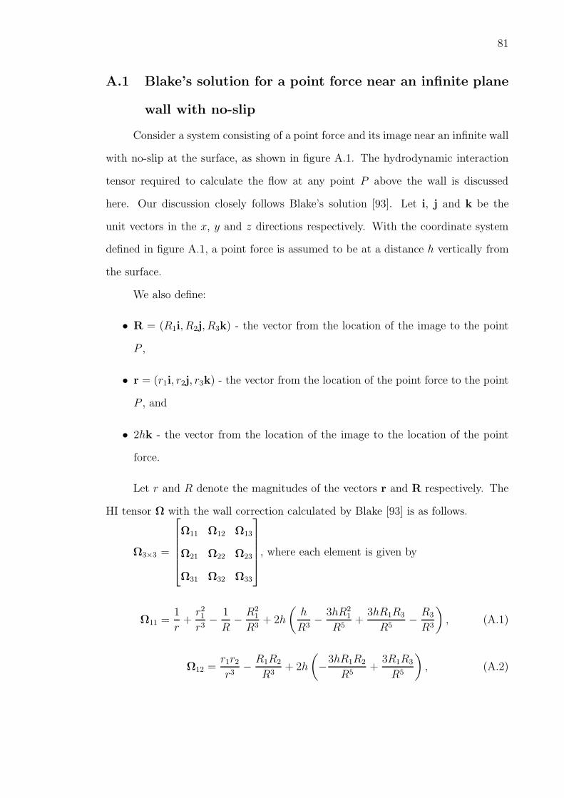
81

A.1 Blake’s solution for a point force near an infinite plane

wall with no-slip

Consider a system consisting of a point force and its image near an infinite wall

with no-slip at the surface, as shown in figure A.1. The hydrodynamic interaction

tensor required to calculate the flow at any point P above the wall is discussed

here. Our discussion closely follows Blake’s solution [93]. Let i, j and k be the

unit vectors in the x, y and z directions respectively. With the coordinate system

defined in figure A.1, a point force is assumed to be at a distance h vertically from

the surface.

We also define:

• R = (R1i, R2j, R3k) - the vector from the location of the image to the point

P ,

• r = (r1i, r2j, r3k) - the vector from the location of the point force to the point

P , and

• 2hk - the vector from the location of the image to the location of the point

force.

Let r and R denote the magnitudes of the vectors r and R respectively. The

HI tensor Ω with the wall correction calculated by Blake [93] is as follows.

Ω3×3 =

Ω11 Ω12 Ω13

Ω21 Ω22 Ω23

Ω31 Ω32 Ω33

, where each element is given by

Ω11 =1

r+r21r3

− 1

R− R2

1

R3+ 2h

(

h

R3− 3hR2

1

R5+

3hR1R3

R5− R3

R3

)

, (A.1)

Ω12 =r1r2r3

− R1R2

R3+ 2h

(

−3hR1R2

R5+

3R1R3

R5

)

, (A.2)

82

Ω13 =r1r3r3

− R1R3

R3− 4h

(

−3hR1R3

R5+

3R1R3

R5− R1

R3

)

, (A.3)

Ω21 =r2r1r3

− R2R1

R3+ 2h

(

−3hR2R1

R5+

3R2R3

R5

)

, (A.4)

Ω22 =1

r+r22r3

− 1

R− R2

2

R3+ 2h

(

h

R3− 3hR2

2

R5+

3hR2R3

R5− R3

R3

)

, (A.5)

Ω23 =r2r3r3

− R2R3

R3− 4h

(

−3hR2R3

R5+

3R2R3

R5− R2

R3

)

, (A.6)

Ω31 =r3r1r3

− R3R1

R3+ 2h

(

−3hR3R1

R5+

3R23

R5+R1

R3

)

, (A.7)

Ω32 =r3r2r3

− R3R2

R3+ 2h

(

−3hR3R2

R5+

3R23

R5− R2

R3

)

, (A.8)

Ω33 =1

r+r23r3

− 1

R− R2

3

R3− 4h

(

h

R3− 3hR2

3

R5+

3R23

R5− R3

R3

)

. (A.9)

We here note that Ω is nonsymmetric and equation (3.31) is used to obtain a

symmetric hydrodynamic interaction tensor.

A.2 Hydrodynamic diffusion tensor for a bead-spring poly-

mer between two walls

This section discusses the description of the HI tensor for our bead-spring

chain polymer model and the stepping in time of the bead positions via Fixman’s

mid-point algorithm [94]. To elucidate the derivation, we here derive the grand

hydrodynamic diffusion tensor (including wall HI) for a simple polymer dumbbell

model leading to a 6×6 diffusion tensor. In our simulations, we extend the derivation

below for an N bead polymer chain, which leads to a 3N × 3N diffusion tensor.

The two beads, labelled (1) and (2), of the polymer dumbbell and their images

in walls A (1a, 2a) and B (1b, 2b) are shown in figure A.2. Multiple (secondary)

reflections from the walls have been ignored here as their contribution is negligible

83

Wall B

Wall A

2b1b

1 2

2a1a

Figure A.2: Illustration of a representative polymer dumbbell, with beads labelled(1) and (2). The images of the polymer in the walls A (1a,2a) and B(1b,2b) are also sketched.

in comparison to the contribution from the first images. The net flow (due to the

wall HI) at the position of the bead (2) is the sum of the flow due to the bead (1),

and the flow due to the images of the beads (1) and (2) in the two walls (1a, 1b,

2a, 2b). The diffusion tensor D of size 6 × 6 is written using the HI tensors (that

are evaluated from equations (A.1) - (A.9)). This diffusion tensor can be written as

D =

D11 D12

D21 D22

, with each element Dij of size 3× 3 representing the flow due to

the beads and the images. The components of D are

D11 = kBT

[

1

ζI+Ω

image1,1a +Ω

image1,1b

]

, (A.10)

D12 = kBT[

ΩOB1,2 +Ω

image1,2a +Ω

image1,2b

]

, (A.11)

D21 = kBT[

ΩOB2,1 +Ω

image2,1a +Ω

image2,1b

]

, (A.12)

84

D22 = kBT

[

1

ζI+Ω

image2,2a +Ω

image2,2b

]

. (A.13)

Here, I is an identity tensor of size 3 × 3. ΩOB/imagep,q represents the appropriate HI

tensor accounting for the force (point-force/image) at location q to evaluate the flow

at location p. Again, D is made symmetric by using a method similar to equations

(3.31) and (3.32).

Therefore, we re-define Dnew12 and Dnew

21 as

Dnew12 =

D12 +DT21

2, (A.14)

Dnew21 =

D21 +DT12

2. (A.15)

From equation (A.14) and (A.15), we have Dnew12 = (Dnew

21 )T .

Therefore, the diffusion tensor defined as D =

D11 Dnew12

Dnew21 D22

is both positive-

definite and symmetric, and can be used in the stochastic differential equation (3.18).

The numerical integration of this equation can be performed without explicitly

calculating the derivative term ∂∂r

·D [91,94]. We use a finite difference approxima-

tion to estimate the first-order derivative term. Equation (3.18) is rewritten as

r∗ = r+√2B(r) ·∆W, (A.16)

∆r =

[

u(r) +D

kBT· Fsys

]

∆t+

√2

2D(r∗)·[(B−1(r))T ·∆W]+

√2

2B(r)·∆W, (A.17)

where ∆W is a vector of independent random variables from a Gaussian distribution

with a zero mean and variance ∆t. The bead-spring polymer is time-stepped using

the above equations.

REFERENCES

[1] D. Wever, F. Picchioni, and A. Broekhuis, “Polymers for enhanced oilrecovery: a paradigm for structure–property relationship in aqueoussolution,” Progress in Polymer Science, vol. 36, no. 11, pp. 1558–1628, 2011.

[2] C. M. White and M. G. Mungal, “Mechanics and prediction of turbulentdrag reduction with polymer additives,” Annual Review of Fluid Mechanics,vol. 40, pp. 235–256, 2008.

[3] A. Alexander-Katz, M. Schneider, S. Schneider, A. Wixforth, and R. Netz,“Shear-flow-induced unfolding of polymeric globules,” Physical ReviewLetters, vol. 97, no. 13, p. 138101, 2006.

[4] S. Schneider, S. Nuschele, A. Wixforth, C. Gorzelanny, A. Alexander-Katz,R. Netz, and M. Schneider, “Shear-induced unfolding triggers adhesion ofvon Willebrand factor fibers,” Proceedings of the National Academy ofSciences, vol. 104, no. 19, pp. 7899–7903, 2007.

[5] X. Zhang, K. Halvorsen, C.-Z. Zhang, W. P. Wong, and T. A. Springer,“Mechanoenzymatic cleavage of the ultralarge vascular protein vonWillebrand factor,” Science, vol. 324, no. 5932, pp. 1330–1334, 2009.

[6] M. Doi and S. Edwards, The Theory of Polymer Dynamics. OxfordUniversity Press, 1986.

[7] R. B. Bird, C. Curtiss, R. Armstrong, and O. Hassager, Dynamics ofPolymeric Liquids, 2 Volume Set. Wiley-Interscience, 1996.

[8] T. T. Perkins, S. R. Quake, D. E. Smith, and S. Chu, “Relaxation of a singleDNA molecule observed by optical microscopy,” Science, vol. 264, no. 5160,pp. 822–825, 1994.

[9] T. T. Perkins, D. E. Smith, R. G. Larson, and S. Chu, “Stretching of a singletethered polymer in a uniform flow,” Science, vol. 268, no. 5207, pp. 83–87,1995.

[10] T. T. Perkins, D. E. Smith, and S. Chu, “Single polymer dynamics in anelongational flow,” Science, vol. 276, no. 5321, pp. 2016–2021, 1997.

[11] D. E. Smith, H. P. Babcock, and S. Chu, “Single-polymer dynamics insteady shear flow,” Science, vol. 283, no. 5408, pp. 1724–1727, 1999.

85

86

[12] P. S. Doyle, B. Ladoux, and J.-L. Viovy, “Dynamics of a tethered polymer inshear flow,” Physical Review Letters, vol. 84, no. 20, pp. 4769–4772, 2000.

[13] C. M. Schroeder, H. P. Babcock, E. S. Shaqfeh, and S. Chu, “Observation ofpolymer conformation hysteresis in extensional flow,” Science, vol. 301,no. 5639, pp. 1515–1519, 2003.

[14] C. M. Schroeder, E. S. Shaqfeh, and S. Chu, “Effect of hydrodynamicinteractions on DNA dynamics in extensional flow: Simulation and singlemolecule experiment,” Macromolecules, vol. 37, no. 24, pp. 9242–9256, 2004.

[15] T. M. Squires and S. R. Quake, “Microfluidics: Fluid physics at the nanoliterscale,” Reviews of Modern Physics, vol. 77, no. 3, pp. 977–1026, 2005.

[16] A. Arora, G. Simone, G. B. Salieb-Beugelaar, J. T. Kim, and A. Manz,“Latest developments in micro total analysis systems,” Analytical Chemistry,vol. 82, no. 12, pp. 4830–4847, 2010.

[17] E. Livak-Dahl, I. Sinn, and M. Burns, “Microfluidic chemical analysissystems,” Annual Review of Chemical and Biomolecular Engineering, vol. 2,no. 1, pp. 325–353, 2011.

[18] S. Haeberle and R. Zengerle, “Microfluidic platforms for lab-on-a-chipapplications,” Lab on a Chip, vol. 7, no. 9, pp. 1094–1110, 2007.

[19] D. Mark, S. Haeberle, G. Roth, F. von Stetten, and R. Zengerle,“Microfluidic lab-on-a-chip platforms: requirements, characteristics andapplications,” Chemical Society Reviews, vol. 39, no. 3, pp. 1153–1182, 2010.

[20] R. N. Zare and S. Kim, “Microfluidic platforms for single-cell analysis,”Annual Review of Biomedical Engineering, vol. 12, no. 1, pp. 187–201, 2010.

[21] Y. Benenson, “Biomolecular computing systems: principles, progress andpotential,” Nature Reviews Genetics, vol. 13, no. 7, pp. 455–468, 2012.

[22] G. M. Church, Y. Gao, and S. Kosuri, “Next-generation digital informationstorage in DNA,” Science, vol. 337, no. 6102, pp. 1628–1628, 2012.

[23] N. C. Stellwagen and E. Stellwagen, “Effect of the matrix on DNAelectrophoretic mobility,” Journal of Chromatography A, vol. 1216, no. 10,pp. 1917–1929, 2009.

[24] N. C. Stellwagen, “Electrophoresis of DNA in agarose gels, polyacrylamidegels and in free solution,” Electrophoresis, vol. 30, no. S1, pp. S188–S195,2009.

[25] J. Herschleb, G. Ananiev, and D. C. Schwartz, “Pulsed-field gelelectrophoresis,” Nature Protocols, vol. 2, no. 3, pp. 677–684, 2007.

87

[26] K. D. Dorfman, S. B. King, D. W. Olson, J. D. Thomas, and D. R. Tree,“Beyond gel electrophoresis: Microfluidic separations, fluorescence burstanalysis, and DNA stretching,” Chemical Reviews, vol. 113, no. 4,pp. 2584–2667, 2012.

[27] R. Godawat, S. N. Jamadagni, and S. Garde, “Characterizinghydrophobicity of interfaces by using cavity formation, solute binding, andwater correlations,” Proceedings of the National Academy of Sciences,vol. 106, no. 36, pp. 15119–15124, 2009.

[28] A. J. Patel, P. Varilly, and D. Chandler, “Fluctuations of water nearextended hydrophobic and hydrophilic surfaces,” The Journal of PhysicalChemistry B, vol. 114, no. 4, pp. 1632–1637, 2010.

[29] A. J. Patel, P. Varilly, S. N. Jamadagni, H. Acharya, S. Garde, andD. Chandler, “Extended surfaces modulate hydrophobic interactions ofneighboring solutes,” Proceedings of the National Academy of Sciences,vol. 108, no. 43, pp. 17678–17683, 2011.

[30] D. Vaknin, W. Bu, and A. Travesset, “Extracting the pair distributionfunction of liquids and liquid-vapor surfaces by grazing incidence x-raydiffraction mode,” The Journal of Chemical Physics, vol. 129, no. 4,p. 044504, 2008.

[31] S. Linse, C. Cabaleiro-Lago, W.-F. Xue, I. Lynch, S. Lindman, E. Thulin,S. E. Radford, and K. A. Dawson, “Nucleation of protein fibrillation bynanoparticles,” Proceedings of the National Academy of Sciences, vol. 104,no. 21, pp. 8691–8696, 2007.

[32] J. Pronchik, X. He, J. T. Giurleo, and D. S. Talaga, “In vitro formation ofamyloid from α-synuclein is dominated by reactions at hydrophobicinterfaces,” Journal of the American Chemical Society, vol. 132, no. 28,pp. 9797–9803, 2010.

[33] W. M. Deen, Analysis of Transport Phenomena. Oxford University Press,New York, 1998.

[34] J. Ennis and L. White, “Electrophoretic Mobility of a Semi-dilute Suspensionof Spherical Particles with Thick Double Layers and Low Zeta Potentials,”Journal of Colloid and Interface Science, vol. 185, no. 1, pp. 157–173, 1997.

[35] D. Long and A. Ajdari, “A note on the screening of hydrodynamicinteractions, in electrophoresis, and in porous media,” The EuropeanPhysical Journal E, vol. 4, no. 1, pp. 29–32, 2001.

[36] J.-L. Barrat and J.-F. Joanny, “Theory of polyelectrolyte solutions,”Advances in Chemical Physics, vol. 94, pp. 1–66, 1997.

88

[37] G. Manning, “Limiting laws and counterion concentration in polyelectrolytesolutions. 7. Electrophoretic mobility and conductance,” Journal of PhysicalChemistry, vol. 85, pp. 1506–1515, 1981.

[38] J.-L. Viovy, “Electrophoresis of DNA and other polyelectrolytes: Physicalmechanisms,” Reviews of Modern Physics, vol. 72, no. 3, pp. 813–872, 2000.

[39] D. Long, J.-L. Viovy, and A. Ajdari, “Simultaneous action of electric fieldsand nonelectric forces on a polyelectrolyte: Motion and deformation,”Physical Review Letters, vol. 76, no. 20, pp. 3858–3861, 1996.

[40] T. Shendruk, O. Hickey, G. Slater, and J. Harden, “Electrophoresis: whenhydrodynamics matter,” Current Opinion in Colloid & Interface Science,vol. 17, no. 2, pp. 74–82, 2012.

[41] R. Kekre, J. E. Butler, and A. J. Ladd, “Role of hydrodynamic interactionsin the migration of polyelectrolytes driven by a pressure gradient and anelectric field,” Physical Review E, vol. 82, no. 5, p. 050803, 2010.

[42] W.-C. Liao, N. Watari, S. Wang, X. Hu, R. G. Larson, and L. J. Lee,“Conformation dependence of DNA electrophoretic mobility in a convergingchannel,” Electrophoresis, vol. 31, no. 16, pp. 2813–2821, 2010.

[43] P. De Gennes, “Molecular individualism,” Science, vol. 276, no. 5321,pp. 1999–2000, 1997.

[44] R. Larson, H. Hu, D. Smith, and S. Chu, “Brownian dynamics simulations ofa DNA molecule in an extensional flow field,” Journal of Rheology, vol. 43,no. 2, pp. 267–304, 1999.

[45] G. Yohannes, M. Jussila, K. Hartonen, and M.-L. Riekkola, “Asymmetricalflow field-flow fractionation technique for separation and characterization ofbiopolymers and bioparticles,” Journal of Chromatography A, vol. 1218,no. 27, pp. 4104–4116, 2011.

[46] B. Roda, A. Zattoni, P. Reschiglian, M. H. Moon, M. Mirasoli, E. Michelini,and A. Roda, “Field-flow fractionation in bioanalysis: a review of recenttrends,” Analytica Chimica Acta, vol. 635, no. 2, pp. 132–143, 2009.

[47] S. K. R. Williams, J. R. Runyon, and A. A. Ashames, “Field-flowfractionation: addressing the nano challenge,” Analytical chemistry, vol. 83,no. 3, pp. 634–642, 2010.

[48] R. N. Qureshi and W. T. Kok, “Application of flow field-flow fractionationfor the characterization of macromolecules of biological interest: a review,”Analytical and Bioanalytical Chemistry, vol. 399, no. 4, pp. 1401–1411, 2011.

89

[49] J. Zheng and E. S. Yeung, “Anomalous radial migration of single DNAmolecules in capillary electrophoresis,” Analytical Chemistry, vol. 74, no. 17,pp. 4536–4547, 2002.

[50] J. Zheng and E. S. Yeung, “Mechanism for the separation of large moleculesbased on radial migration in capillary electrophoresis,” Analytical Chemistry,vol. 75, no. 15, pp. 3675–3680, 2003.

[51] J. Zheng and E. S. Yeung, “Counting single DNA molecules in a capillarywith radial focusing,” Australian Journal of Chemistry, vol. 56, no. 3,pp. 149–153, 2003.

[52] J. Zheng, H.-W. Li, and E. S. Yeung, “Manipulation of single DNAmolecules via lateral focusing in a PDMS/glass microchannel,” The Journalof Physical Chemistry B, vol. 108, no. 29, pp. 10357–10362, 2004.

[53] O. B. Usta, J. E. Butler, and A. J. Ladd, “Transverse migration of aconfined polymer driven by an external force,” Physical Review Letters,vol. 98, no. 9, p. 098301, 2007.

[54] J. E. Butler, O. B. Usta, R. Kekre, and A. J. Ladd, “Kinetic theory of aconfined polymer driven by an external force and pressure-driven flow,”Physics of Fluids, vol. 19, no. 11, p. 113101, 2007.

[55] G. C. Randall, K. M. Schultz, and P. S. Doyle, “Methods toelectrophoretically stretch DNA: microcontractions, gels, and hybridgel-microcontraction devices,” Lab on a Chip, vol. 6, no. 4, pp. 516–525,2006.

[56] J. Tang and P. S. Doyle, “Electrophoretic stretching of DNA molecules usingmicroscale T junctions,” Applied Physics Letters, vol. 90, no. 22,pp. 224103–224103, 2007.

[57] A. G. Balducci, J. Tang, and P. S. Doyle, “Electrophoretic stretching of dnamolecules in cross-slot nanoslit channels,” Macromolecules, vol. 41, no. 24,pp. 9914–9918, 2008.

[58] E. Y. Chan, N. M. Goncalves, R. A. Haeusler, A. J. Hatch, J. W. Larson,A. M. Maletta, G. R. Yantz, E. D. Carstea, M. Fuchs, G. G. Wong, et al.,“DNA mapping using microfluidic stretching and single-molecule detectionof fluorescent site-specific tags,” Genome research, vol. 14, no. 6,pp. 1137–1146, 2004.

[59] E. Protozanova, M. Zhang, E. J. White, E. T. Mollova, D. T. Broeck, S. V.Fridrikh, D. B. Cameron, and R. Gilmanshin, “Fast high-resolution mappingof long fragments of genomic DNA based on single-molecule detection,”Analytical Biochemistry, vol. 402, no. 1, pp. 83–90, 2010.

90

[60] R. H. Meltzer, J. R. Krogmeier, L. W. Kwok, R. Allen, B. Crane, J. W.Griffis, L. Knaian, N. Kojanian, G. Malkin, M. K. Nahas, et al., “Alab-on-chip for biothreat detection using single-molecule DNA mapping,”Lab on a Chip, vol. 11, no. 5, pp. 863–873, 2011.

[61] M. Tanyeri, E. M. Johnson-Chavarria, and C. M. Schroeder, “Hydrodynamictrap for single particles and cells,” Applied Physics Letters, vol. 96, no. 22,pp. 224101–224101, 2010.

[62] A. E. Cohen and W. Moerner, “Suppressing Brownian motion of individualbiomolecules in solution,” Proceedings of the National Academy of Sciencesof the United States of America, vol. 103, no. 12, pp. 4362–4365, 2006.

[63] Q. Wang and W. Moerner, “Optimal strategy for trapping single fluorescentmolecules in solution using the ABEL trap,” Applied Physics B, vol. 99,no. 1-2, pp. 23–30, 2010.

[64] M. Tanyeri, M. Ranka, N. Sittipolkul, and C. M. Schroeder, “Amicrofluidic-based hydrodynamic trap: design and implementation,” Lab ona Chip, vol. 11, no. 10, pp. 1786–1794, 2011.

[65] M. Tanyeri and C. M. Schroeder, “Manipulation and Confinement of SingleParticles Using Fluid Flow,” Nano letters, vol. 13, no. 6, p. 23572364, 2013.

[66] K. C. Neuman and A. Nagy, “Single-molecule force spectroscopy: opticaltweezers, magnetic tweezers and atomic force microscopy,” Nature Methods,vol. 5, no. 6, p. 491, 2008.

[67] T. T. Perkins, “Optical traps for single molecule biophysics: a primer,” Laser& Photonics Reviews, vol. 3, no. 1-2, pp. 203–220, 2009.

[68] C. L. Asbury, A. H. Diercks, G. van den Engh, et al., “Trapping of DNA bydielectrophoresis,” Electrophoresis, vol. 23, no. 16, pp. 2658–2666, 2002.

[69] R. Dylla-Spears, J. E. Townsend, L. Jen-Jacobson, L. L. Sohn, and S. J.Muller, “Single-molecule sequence detection via microfluidic planarextensional flow at a stagnation point,” Lab on a Chip, vol. 10, no. 12,pp. 1543–1549, 2010.

[70] W. Liu, L. Li, J.-c. Wang, Q. Tu, L. Ren, Y. Wang, and J. Wang, “Dynamictrapping and high-throughput patterning of cells using pneumaticmicrostructures in an integrated microfluidic device,” Lab on a Chip, vol. 12,no. 9, pp. 1702–1709, 2012.

[71] W. Xu and S. J. Muller, “Polymer-monovalent salt-induced DNAcompaction studied via single-molecule microfluidic trapping,” Lab on aChip, vol. 12, no. 3, pp. 647–651, 2012.

91

[72] A. D. Dinsmore, J. C. Crocker, and A. G. Yodh, “Self-assembly of colloidalcrystals,” Current Opinion in Colloid & Interface Science, vol. 3, no. 1,pp. 5–11, 1998.

[73] Y. Xia, B. Gates, Y. Yin, and Y. Lu, “Monodispersed colloidal spheres: oldmaterials with new applications,” Advanced Materials, vol. 12, no. 10,pp. 693–713, 2000.

[74] S. C. Glotzer and M. J. Solomon, “Anisotropy of building blocks and theirassembly into complex structures,” Nature materials, vol. 6, no. 8,pp. 557–562, 2007.

[75] C. Tanford, Ben Franklin stilled the waves: An informal history of pouringoil on water with reflections on the ups and downs of scientific life ingeneral. Oxford University Press, 2004.

[76] M. L. Schlossman, “Liquid–liquid interfaces: studied by X-ray and neutronscattering,” Current Opinion in Colloid & Interface Science, vol. 7, no. 3,pp. 235–243, 2002.

[77] D. Schwartz, M. Schlossman, E. Kawamoto, G. Kellogg, P. S. Pershan, andB. Ocko, “Thermal diffuse x-ray-scattering studies of the water-vaporinterface,” Physical Review A, vol. 41, pp. 5687–5690, 1990.

[78] J. Alejandre, D. J. Tildesley, and G. A. Chapela, “Molecular dynamicssimulation of the orthobaric densities and surface tension of water,” TheJournal of chemical physics, vol. 102, no. 11, pp. 4574–4583, 1995.

[79] R. Radhakrishnan and P. T. Underhill, “Impact of solvent quality on thehysteresis in the coil–stretch transition of flexible polymers in goodsolvents,” Macromolecules, vol. 46, no. 2, pp. 548–554, 2012.

[80] A. Cohen, “A Pade approximant to the inverse Langevin function,”Rheologica Acta, vol. 30, no. 3, pp. 270–273, 1991.

[81] D. L. Ermak and J. A. McCammon, “Brownian dynamics withhydrodynamic interactions,” The Journal of Chemical Physics, vol. 69, no. 4,pp. 1352–1360, 1978.

[82] P. Grassia, E. Hinch, and L. Nitsche, “Computer simulations of Brownianmotion of complex systems,” Journal of Fluid Mechanics, vol. 282,pp. 373–403, 1995.

[83] R. M. Jendrejack, J. J. de Pablo, and M. D. Graham, “Stochasticsimulations of DNA in flow: Dynamics and the effects of hydrodynamicinteractions,” The Journal of Chemical Physics, vol. 116, p. 7752, 2002.

92

[84] C.-C. Hsieh, L. Li, and R. G. Larson, “Modeling hydrodynamic interactionin Brownian dynamics: simulations of extensional flows of dilute solutions ofDNA and polystyrene,” Journal of Non-Newtonian Fluid Mechanics,vol. 113, no. 2, pp. 147–191, 2003.

[85] J. S. Hur, E. S. Shaqfeh, and R. G. Larson, “Brownian dynamics simulationsof single DNA molecules in shear flow,” Journal of Rheology, vol. 44, p. 713,2000.

[86] R. Kekre, J. E. Butler, and A. J. Ladd, “Comparison of lattice-Boltzmannand Brownian-dynamics simulations of polymer migration in confined flows,”Physical Review E, vol. 82, no. 1, p. 011802, 2010.

[87] H. R. Warner Jr, “Kinetic theory and rheology of dilute suspensions offinitely extendible dumbbells,” Industrial & Engineering ChemistryFundamentals, vol. 11, no. 3, pp. 379–387, 1972.

[88] C. W. Oseen, Hydrodynamik, vol. 1. Akad. Verl.-Ges., 1927.

[89] J. Burgers, “Second report on viscosity and plasticity,” Academy of Sciences,Amsterdam, 1938.

[90] C. Pozrikidis, Introduction to theoretical and computational fluid dynamics.Oxford University Press, 2011.

[91] R. M. Jendrejack, D. C. Schwartz, J. J. de Pablo, and M. D. Graham,“Shear-induced migration in flowing polymer solutions: Simulation oflong-chain DNA in microchannels,” The Journal of Chemical Physics,vol. 120, p. 2513, 2004.

[92] B. Felderhof, “Diffusion of interacting Brownian particles,” Journal ofPhysics A: Mathematical and General, vol. 11, no. 5, p. 929, 1978.

[93] J. Blake, “A note on the image system for a stokeslet in a no-slip boundary,”in Proc. Camb. Phil. Soc, vol. 70, pp. 303–310, Cambridge Univ Press, 1971.

[94] M. Fixman, “Implicit algorithm for Brownian dynamics of polymers,”Macromolecules, vol. 19, no. 4, pp. 1195–1204, 1986.

[95] D. Heyes and J. Melrose, “Brownian dynamics simulations of modelhard-sphere suspensions,” Journal of Non-Newtonian Fluid Mechanics,vol. 46, no. 1, pp. 1–28, 1993.

[96] C. M. Soto and B. R. Ratna, “Virus hybrids as nanomaterials forbiotechnology,” Current Opinion in Biotechnology, vol. 21, no. 4,pp. 426–438, 2010.

93

[97] J. K. Pokorski and N. F. Steinmetz, “The art of engineering viralnanoparticles,” Molecular Pharmaceutics, vol. 8, no. 1, pp. 29–43, 2010.

[98] D. E. Cliffel, B. N. Turner, and B. J. Huffman, “Nanoparticle-based biologicmimetics,” Wiley Interdisciplinary Reviews: Nanomedicine andNanobiotechnology, vol. 1, no. 1, pp. 47–59, 2009.

[99] P. D. Grossman and D. S. Soane, “Orientation effects on the electrophoreticmobility of rod-shaped molecules in free solution,” Analytical Chemistry,vol. 62, no. 15, pp. 1592–1596, 1990.

[100] H. Z. Cummins, F. D. Carlson, T. J. Herbert, and G. Woods, “Translationaland rotational diffusion constants of tobacco mosaic virus from Rayleighlinewidths,” Biophysical Journal, vol. 9, no. 4, pp. 518–546, 1969.

[101] C.-C. Hsieh, S. Jain, and R. G. Larson, “Brownian dynamics simulationswith stiff finitely extensible nonlinear elastic-Fraenkel springs asapproximations to rods in bead-rod models,” The Journal of ChemicalPhysics, vol. 124, no. 4, p. 044911, 2006.

[102] Y. Xia and G. M. Whitesides, “Soft lithography,” Annual Review ofMaterials Science, vol. 28, no. 1, pp. 153–184, 1998.

[103] D. Qin, Y. Xia, and G. M. Whitesides, “Soft lithography for micro-andnanoscale patterning,” Nature Protocols, vol. 5, no. 3, pp. 491–502, 2010.

[104] J. M. Sidorova, N. Li, D. C. Schwartz, A. Folch, and R. J. Monnat Jr,“Microfluidic-assisted analysis of replicating DNA molecules,” NatureProtocols, vol. 4, no. 6, pp. 849–861, 2009.

[105] J. A. Rogers and R. G. Nuzzo, “Recent progress in soft lithography,”Materials Today, vol. 8, no. 2, pp. 50–56, 2005.

[106] J. C. Crocker and D. G. Grier, “Methods of digital video microscopy forcolloidal studies,” Journal of Colloid and Interface Science, vol. 179, no. 1,pp. 298–310, 1996.

[107] J. C. Crocker and B. D. Hoffman, “Multiple-Particle Tracking and Two-PointMicrorheology in Cells,” Methods in Cell Biology, vol. 83, pp. 141–178, 2007.

[108] D. Frenkel and B. Smit, Understanding molecular simulation: fromalgorithms to applications, vol. 1. Academic Press, 2001.

[109] G. C. Randall, Single molecule analysis of DNA electrophoresis inmicrodevices. PhD thesis, Massachusetts Institute of Technology, 2006.

94

[110] E. A. Doherty, K. D. Berglund, B. A. Buchholz, I. V. Kourkine, T. M.Przybycien, R. D. Tilton, and A. E. Barron, “Critical factors forhigh-performance physically adsorbed (dynamic) polymeric wall coatings forcapillary electrophoresis of DNA,” Electrophoresis, vol. 23, no. 16,pp. 2766–2776, 2002.

[111] C. F. Duffy, A. A. McEathron, E. A. Arriaga, et al., “Determination ofindividual microsphere properties by capillary electrophoresis withlaser-induced fluorescence detection,” Electrophoresis, vol. 23, no. 13,p. 2040, 2002.

[112] B. Xiong, A. Pallandre, I. le Potier, P. Audebert, E. Fattal, N. Tsapis,G. Barratt, and M. Taverna, “Electrophoretic mobility measurement by laserDoppler velocimetry and capillary electrophoresis of micrometric fluorescentpolystyrene beads,” Analytical Methods, vol. 4, no. 1, pp. 183–189, 2012.

[113] W. Humphrey, A. Dalke, and K. Schulten, “VMD – Visual MolecularDynamics,” Journal of Molecular Graphics, vol. 14, pp. 33–38, 1996.

[114] L. Li and S. Garde, “Binding, structure, and dynamics of hydrophobicpolymers near patterned self-assembled monolayer surfaces,” Langmuir,vol. 30, no. 47, pp. 14204–14211, 2014.

[115] J. F. Marko and E. D. Siggia, “Stretching dna,” Macromolecules, vol. 28,no. 26, pp. 8759–8770, 1995.