Final Technical Report

for

SERDP Project CU-1064

Bioenhanced In-well Vapor Stripping (BEHIVS) to Treat Trichloroethylene

February 2003

1

1. Project title: Bioenhanced In-well Vapor Stripping (BEHIVS) to Treat Trichloroethylene 2. Performing organizations: Western Region Hazardous Substance Research Center

(Stanford University) Air Force Institute of Technology

3. Project background: This project is focussed on remediating the source area of trichloroethylene (TCE)-contaminated groundwater. TCE is the most commonly detected groundwater contaminant at DoD and Superfund sites. Low-cost alternatives for treating the source of TCE-contamination are needed, preferably ones not requiring the removal of contaminated water from the subsurface. 4. Objective: The overall project objective is to demonstrate the potential of combining two innovative, recently demonstrated, remediation technologies, in-well vapor stripping (IWVS) and in situ aerobic cometabolic bioremediation, to cleanup a TCE source area without having to bring contaminated groundwater to the surface. The combination of vapor stripping and bioremediation technologies will be referred to by the term bioenhanced in-well vapor stripping (BEHIVS). 5. Technical approach: Under this project, an in-well vapor stripper and two biotreatment wells were installed near a TCE contaminated "hot spot zone" at Edwards AFB (Figure 1). In operation, the in-well vapor stripper used air- lift pumping to pump contaminated water from the lower portion of the aquifer to a screened interval above and below the water table. The TCE was stripped out of the water into the gas phase, which was subsequently treated using granular activated carbon. The treated water leaving the upper screen of the in-well vapor stripper flowed to the upper screen of the biotreatment wells. Water entering the biotreatment wells was pumped down through the wells, where a primary substrate (toluene), and oxygen were added. After addition of the primary substrate and oxygen the water was injected into the aquifer through the lower screened intervals, where indigenous microorganisms aerobically metabolized the primary substrate and cometabolized the contaminant. Water leaving the bioactive zone recirculated back to the lower screen of the in-well vapor stripper for further treatment. Note that a recirculation system was established between the upflow vapor stripping well and the downflow biotreatment wells. The high concentrations of dissolved TCE entering the vapor stripping well volatilized and the TCE-rich vapor was removed, while the biotreatment well served as a "polishing" step, further reducing contaminant concentrations to very low levels. We believe the combined technology of bioenhanced in-well vapor stripping will remove as much or more of the TCE near the source than would be removed compared to conventional technologies (e.g., pump-and-treat). If one assumes >90% reduction of concentration in the in-well vapor stripper, >90% reduction in the bioactive zone, and that the treated water undergoes substantial recirculation between the upflow and downflow wells, more than two orders of magnitude reduction in contaminant concentration will be achieved for groundwater undergoing combined treatment. In addition, the TCE mass in the source area will be reduced due to local heavy treatment and recirculation near the vapor-stripping well.

2

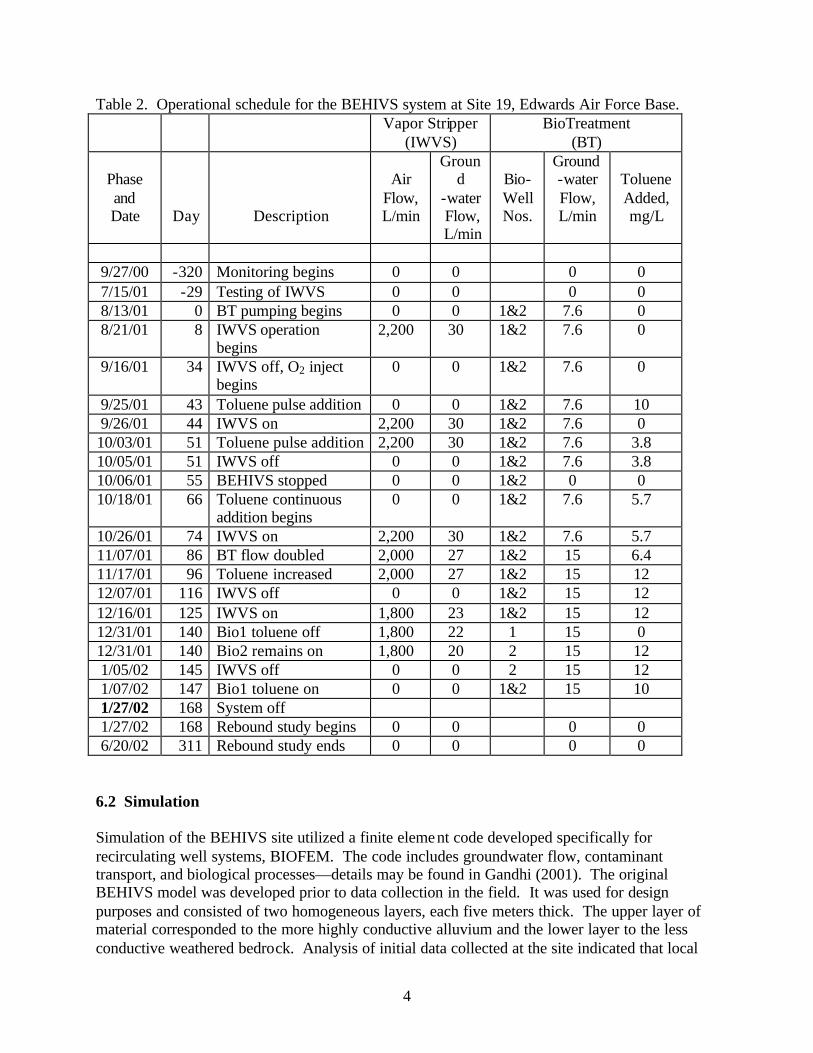
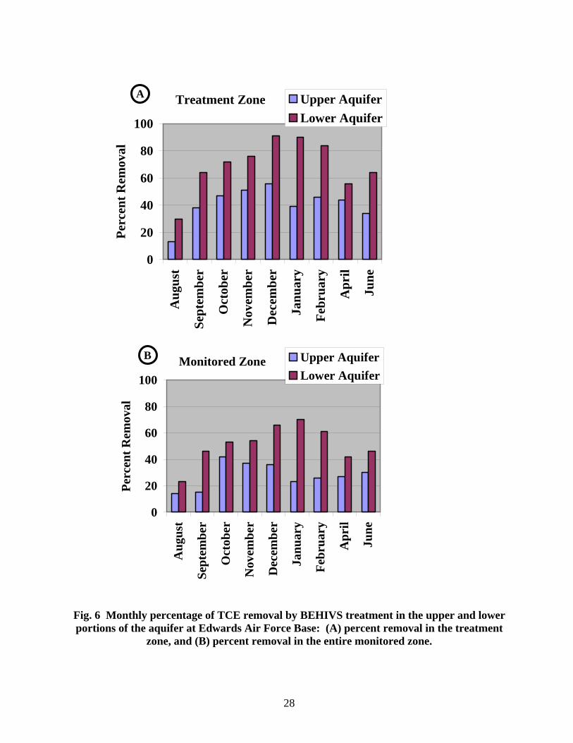
Operation of the technology was monitored using an extensive system of wells (Figure 2), connected to an automated sampling and analysis system (Figure 3). This monitoring technique has proven capable of inexpensively providing the large amounts of quality data needed to monitor the performance of an in situ remediation technology. 6. Summary of Final Product The primary product resulting from this project is a dataset from the field evaluation. This dataset was analyzed using a numerical model that simulated application of the BEHIVS technology at the evaluation site. 6.1 Overall System Results The overall removals effected during the BEHIVS operation between August 13, 2001, and December 27, 2001, a period of four and one-half months, are shown in Table 1. The vapor stripping well pumped at an average rate of 6.9 gpm. The bioremediation wells pumped at 2.0 gpm for the first 86 days of operation and at 4.0 gpm for the remainder of the time. The monitored region was approximately 48 m by 56 m (see Figure 4). As shown in the figure, the monitoring-well layout was designed to collect data both inside and outside the treatment area. Also, as shown in Figure 4, the active treatment area was approximately 32 m by 42 m, and contained 14 monitoring wells that provided 28 locations with data for the upper and lower aquifer zones. Within the BEHIVS treatment area, the average TCE concentration reduction in the lower aquifer zone was 91 percent, with a reduction of 94 to 97 percent at 10 of the 14 monitoring wells. Average TCE removals in the treatment area exceeded 56% in the upper aquifer zone, with 3 monitoring well showing a reduction greater than 92%. As shown in Figure 5, from August 16, 2001 through December 27, 2001 the TCE stripping ratio for the vapor stripping well averaged 95.4%. Overall for the entire study area, including that area outside the treatment area, average TCE removals were 70 percent in the lower aquifer zone and 38 percent in the upper aquifer zone. Those values for the entire study area include a significant region outside of the treatment zone and therefore the average removal percentages are not as high as those within the treatment zone. Figure 6 displays the monthly percentage concentration changes, which showed consistent reductions (mass removal) from system startup through January 2002 when the vapor-stripping well was shut off. The total TCE mass removal was 8.1 kg, 7.1 kg of which resulted from vapor stripping and 1.0 kg from biotreatment. Mass removal rates are illustrated in Figure 7 due to vapor-stripping and Figure 8 due to in situ biological treatment. Additional details are shown in the attached Final Report: Operation and Analysis of the BEHIVS System at Edwards Air Force Base, 18 February 2003 (WRHSRC, 2003). After the BEHIVS demonstration period, a five month period of monitoring was conducted to assess rebound of concentrations. This “rebound study” was useful in identifying TCE source areas in the fractured bedrock. The monitoring and operation schedule beginning 9/27/00 and ending 6/20/02 is shown in Table 2.

3

Table 1. Average TCE concentrations measured at various sampling locations showing comparisons between pre-operational TCE concentrations and those during December 2001. Bold values are monitoring locations within the treatment zone. n is the number of samples. Upper Aquifer Zone Lower Aquifer Zone

December Results

Pre-Operational

December Results

Pre-Operational

Average Average Change Average Average Change Well n (µg/L) (µg/L) (Percent) n (µg/L) (µg/L) (Percent)

D04-C 7 1479 4960 -70% Bio1 22 495 659 -25% 28 432 6862 -94% Bio2 11 311 608 -49% 13 320 4982 -94% N-01 6 658 815 -19% 9 4613 6955 -34% N-02 8 193 797 -76% 9 2217 2475 -10% N-03 6 450 927 -51% 8 2756 3352 -18% N-04 11 347 1322 -80% 57 2125 8273 -74% N-05 8 742 1000 -26% 7 191 6056 -97% N-06 9 859 1323 -35% 14 2768 3450 -20% N-07 11 66 808 -92% 27 142 4574 -97% N-08 12 60 2932 -98% 9 184 5637 -97% N-09 12 56 810 -93% 14 488 4209 -88% N-10 6 442 1109 -60% 25 208 3718 -94% N-11 5 443 1051 -58% 10 192 3823 -95% N-12 5 927 2317 -60% 7 203 3684 -94% N-13 5 287 459 -37% 15 2669 4169 -36% N-14 5 1658 1136 46% 13 751 5117 -85% N-15 6 1556 690 126% 5 2911 5001 -42% N-16 7 528 932 -43% 10 2552 4677 -45% N-17 6 610 775 -21% 12 2083 3694 -44% N-18 6 2048 1568 31% 11 1141 4959 -77% N-19 7 1900 2178 -13% 7 1244 3516 -65% N-20 6 2134 2256 -5% 8 2689 3090 -13% MW21 10 67 616 -89% 23 241 4278 -94% MW22 5 1460 1533 -5% 7 1460 3305 -56% MW23 6 532 919 -42% 25 297 5075 -94%

Average Reduction in

Treatment Zone

473

1176

-56%

518

5089

-91%

Average Change for Entire

Monitored Area

760 1236 -38% 1398 4611 -70%

4

Table 2. Operational schedule for the BEHIVS system at Site 19, Edwards Air Force Base. Vapor Stripper

(IWVS) BioTreatment

(BT)

Phase and Date

Day

Description

Air

Flow, L/min

Ground

-water Flow, L/min

Bio- Well Nos.

Ground-water Flow, L/min

Toluene Added, mg/L

9/27/00 -320 Monitoring begins 0 0 0 0 7/15/01 -29 Testing of IWVS 0 0 0 0 8/13/01 0 BT pumping begins 0 0 1&2 7.6 0 8/21/01 8 IWVS operation

begins 2,200 30 1&2 7.6 0

9/16/01 34 IWVS off, O2 inject begins

0 0 1&2 7.6 0

9/25/01 43 Toluene pulse addition 0 0 1&2 7.6 10 9/26/01 44 IWVS on 2,200 30 1&2 7.6 0 10/03/01 51 Toluene pulse addition 2,200 30 1&2 7.6 3.8 10/05/01 51 IWVS off 0 0 1&2 7.6 3.8 10/06/01 55 BEHIVS stopped 0 0 1&2 0 0 10/18/01 66 Toluene continuous

addition begins 0 0 1&2 7.6 5.7

10/26/01 74 IWVS on 2,200 30 1&2 7.6 5.7 11/07/01 86 BT flow doubled 2,000 27 1&2 15 6.4 11/17/01 96 Toluene increased 2,000 27 1&2 15 12 12/07/01 116 IWVS off 0 0 1&2 15 12 12/16/01 125 IWVS on 1,800 23 1&2 15 12 12/31/01 140 Bio1 toluene off 1,800 22 1 15 0 12/31/01 140 Bio2 remains on 1,800 20 2 15 12 1/05/02 145 IWVS off 0 0 2 15 12 1/07/02 147 Bio1 toluene on 0 0 1&2 15 10 1/27/02 168 System off 1/27/02 168 Rebound study begins 0 0 0 0 6/20/02 311 Rebound study ends 0 0 0 0

6.2 Simulation Simulation of the BEHIVS site utilized a finite element code developed specifically for recirculating well systems, BIOFEM. The code includes groundwater flow, contaminant transport, and biological processes—details may be found in Gandhi (2001). The original BEHIVS model was developed prior to data collection in the field. It was used for design purposes and consisted of two homogeneous layers, each five meters thick. The upper layer of material corresponded to the more highly conductive alluvium and the lower layer to the less conductive weathered bedrock. Analysis of initial data collected at the site indicated that local

5

flow conditions could not be adequately represented with a model consisting of simple homogeneous layers, so significant effort was aimed at developing a proper model of the hydrogeology of the site. The non-pumping head measurements taken within the lower aquifer (see Figure 9) suggest two differing local gradient directions. One is a northwest to southeast gradient in the northern portion of the treatment area and the other is a slight southwest to -northeast gradient in the southern portion. Funneling of groundwater is likely controlled by a preferred flow pathway in the lower layer. The tracer test data further confirmed the likely existence of the relative preferred pathway and suggested the need to include aquifer heterogeneity in the site model. The development of a new conceptual model of the BEHIVS site was an iterative process, incorporating new data as it became available. This task entailed hundreds of model runs exploring the effects of various hydrogeologic features before the final conceptual model was adopted. The final BEHIVS model is described in the following subsections. 6.2.1 Model grid geometry The BEHIVS model covers a domain of 200 by 200 meters, which is larger than the coverage of the monitoring system but was needed to reduce boundary effects. The finite-element mesh consists of 26,726 nodes and 49,205 elements over 13 vertical layers. Mesh discretization in plan view is highest near the treatment/pumping wells (~20 cm) and coarsest (up to 20 m) approaching the boundaries, with vertical discretization ranging from 1 m at shallow depths to 5 meters near the base of the system. The BEHIVS finite-element model grid is shown in plan view in Figure 10. The model grid covers 20 meters in the vertical, from the water table, which is about 4 m below ground surface, to the bottom of the IWVS lower wellscreen (685-665 meters relative to mean surface level, msl). Each layer potentially consists of five spatially variable material types, with the alluvium occupying the top layers, competent bedrock occupying the bottom layer, and the remaining materials occupying the middle layers:

• Alluvium: This material is located in the upper portion of the aquifer and cons ists of sands and gravels with interspersed clay layers. This material is highly anisotropic in the vertical.

• WBr: The weathered bedrock is located in the lower portion of the aquifer. This material is modeled as isotropic.

• Low K Zone: This material represents areas of lower hydraulic conductivity (K) within the weathered bedrock. The geometry of this material determines the shape of the flow field at the level of the lower wellscreens.

• Channel: This material represents a highly fractured/more conductive area within the weathered bedrock that runs between biotreatment well two and monitoring location N05.

• CBr: The competent bedrock consisting primarily of quartz monzonite is located at the very bottom of the modeled area, at a depth of about 15 m. This material has the lowest conductivity of all model materials.

6

Well boring logs from the 36 wells in the treatment area as well as those of 13 additional wells just outside of the area were examined to determine the location of the competent bedrock (CBr) and the interface between the weathered bedrock (WBr) and the upper alluvium. These data were kriged onto the model grid and used to create material zones, each type having its own hydraulic conductivity value. The interface between the weathered bedrock and the competent bedrock varies from 678 to 675 meters within the BEHIVS treatment area. The elevation of the contact between the weathered bedrock and the alluvium (the upper and lower aquifer materials) varies by approximately three meters in the vertical. Thus the thickness of both the alluvium and weathered bedrock is quite variable. The spatial configuration of material types right around the treatment area in each of the 13 model layers is shown in Figures 11 through 15, which were based on both well logs and simulation analyses. 6.2.2 Initial and Boundary Conditions The BEHIVS model requires initial conditions for all modeled constituents. These include bromide, dissolved oxygen, toluene, TCE, and initial biomass. Prior to the beginning of the first tracer injection, bromide measurements were taken at all but a handful of monitoring wells. Due to high levels of chloride present in the aquifer, bromide measurements are thought to be accurate to +/- 50 mg/L. The initial mean bromide concentration was 17 mg/L, ranging from a low of less than 1 mg/L to a high of 47 mg/L. Since the spatial coverage of these data is not complete, a single initial value of 17 mg/L for bromide was used at all model locations. For dissolved oxygen and TCE, many measurements were available allowing for spatially variable initial conditions. Measurements of each taken in the week prior to system startup (i.e., the first week of August) were kriged onto the model grid creating initial condition maps. Figure16 shows the initial TCE concentration used for the upper and lower aquifers, respectively. Where data were absent, such as outside the highly monitored area, initial conditions were developed based on solute appearing inside the domain later in time. In these upgradient areas, deduced zones of low concentration were added to constrain the kriged values. In the deep bedrock, hotspots are present around monitoring well N04 and between biotreatment well one and N07 and were accounted for in the initial conditions. Figure 17 shows the initial dissolved oxygen concentrations used in the upper and lower aquifers, respectively. As would be expected, dissolved oxygen levels in the weathered bedrock are significantly lower than those in the alluvium. The initial biomass was represented using a nominal seed value to represent conditions prior to the addition of toluene and oxygen. The model domain was purposely made large to minimize the effects of boundary conditions on flow and transport processes within the BEHIVS treatment area. The east and west border of the model domain are constant head (type I) boundaries and the north and south borders are zero-gradient or no-flow (type II) boundaries. The heads used for the constant head boundaries were developed from the initial conditions (e.g., July 27, 2001) observed in the BEHIVS head field. The solute boundary conditions are zero concentration gradient or “advective flux only” across the model boundaries.

7

6.2.3 Modeling of Well Operations Each of the three recirculating treatment wells is modeled as a set of two connected wellscreens, one pumping and one injecting. Pumping/injection rates at the wells varied throughout the BEHIVS demonstration. The model contains a total of 34 successive steady state pumping regimes (see section 5.3 of WRHSRC, 2003 for details). In addition to the treatment wells, we monitored 26 dual-screened wells for head and concentration data. An additional source of water that was accounted for in the model was the sampling return flow from the ASAP (monitoring system) that was injected into the treatment wells. This return flow reached a maximum of about 0.5 gpm during the tracer tests. Sampling return flow is shown in Figure 18. From the beginning of operations through January 9, 2002, this water was injected equally into the biotreatment wells. After January 9 (day 149), this water was added to the infiltration originating from the vapor stripping well. Consequently, the pumping rates measured within the wells reflect a combina tion of the pumped water and the sampling return water. The flowrates modeled at the pumping screens are less than that at the injection screens, by the amount of the return flow. The pumping regimes and the corresponding pumping rates used in the model are given in Table 3. The relative effective pumping rates at the biotreatment wells (i.e., the rate at biotreatment well one as opposed to biotreatment well two) determine the location of stagnation points between them. Thus the local direction of flow is very much dependent on these rates. For example, monitoring wells N09, N14, and N18 received tracer from bioremediation well two, but not from bioremediation well one. 6.2.4 Injection Schedules Oxygen addition at the biotreatment wells began on September 16 and continued throughout well operation. Additionally, the water coming through the vapor stripper was oxygenated by exposure to air. Measurements of dissolved oxygen taken throughout the treatment period were used in the model as oxygen source concentrations at both of the biotreatment wells and the vapor stripping well. Peroxide was injected at both biotreatment wells starting on November 7. The modeled concentration at the injection wellscreens is constant at 45 mg/L until January 27. At the vapor stripping well, peroxide addition began on November 30. The measured oxygen concentrations, which implicitly accounts for all oxygen additions, were used in the model so it was not necessary to explicitly include peroxide as an additional oxygen source. Regular toluene injections began at the biotreatment wells on October 18. The initial schedule included one pulse to each well every two hours. On October 26, the delivery schedule was changed to one pulse to each well every twelve hours. From November 7 through the duration of biotreatment well operation, the delivery schedule was one pulse per well per day. The BEHIVS model averages toluene injections over one-day intervals. The toluene injection concentrations used in the model are shown in Table 4 and are based on the total mass delivered each day.

8

Table 3: Steady state pumping regimes for BEHIVS treatment system (Day 0 is August 13, 2001, and Day 167 is January 27, 2002).

DATE DAY

RETURN FLOW GPM

BIO 1 TOP GPM

BIO 1 BOTTOM

GPM

BIO 2 TOP GPM

BIO 2 BOTTOM

GPM

IWVS TOP GPM

IWVS BOTTOM

GPM

8/13/2001 0.0 0.28 2.36 2.50 2.36 2.50 8.75 8.758/13/2001 0.1 0.28 2.36 2.50 2.36 2.50 0.00 0.008/15/2001 2.2 0.28 1.86 2.00 1.86 2.00 6.50 6.508/15/2001 2.2 0.28 1.86 2.00 1.86 2.00 0.00 0.008/16/2001 3.1 0.28 2.16 2.30 2.16 2.30 6.60 6.608/17/2001 4.1 0.00 0.00 0.00 0.00 0.00 0.00 0.008/21/2001 8.0 0.28 1.86 2.00 1.86 2.00 7.70 7.709/11/2001 29.0 0.28 1.86 2.00 1.86 2.00 0.00 0.009/13/2001 30.9 0.28 1.86 2.00 1.86 2.00 7.93 7.939/16/2001 34.0 0.28 1.86 2.00 1.86 2.00 0.00 0.009/26/2001 44.0 0.27 0.00 0.14 0.00 0.14 0.00 0.009/27/2001 44.8 0.30 0.00 0.15 0.00 0.15 7.72 7.729/28/2001 46.0 0.31 1.85 2.00 0.00 0.15 7.54 7.549/28/2001 46.2 0.31 0.00 0.15 0.00 0.15 7.54 7.549/30/2001 48.0 0.30 1.85 2.00 0.00 0.15 7.58 7.589/30/2001 48.2 0.30 0.00 0.15 0.00 0.15 7.45 7.4510/3/2001 51.0 0.33 1.84 2.00 1.84 2.00 0.00 0.0010/7/2001 55.0 0.30 0.00 0.15 0.00 0.15 0.00 0.0010/18/2001 66.0 0.29 1.85 2.00 1.85 2.00 0.00 0.0010/26/2001 74.0 0.25 1.87 2.00 1.87 2.00 7.77 7.7710/31/2001 78.9 0.39 1.80 2.00 1.80 2.00 7.26 7.2611/7/2001 85.9 0.45 3.78 4.00 3.78 4.00 7.26 7.2611/14/2001 92.9 0.37 3.82 4.00 3.82 4.00 7.18 7.1811/21/2001 99.9 0.39 3.81 4.00 3.81 4.00 6.80 6.8011/28/2001 107.2 0.45 3.78 4.00 3.78 4.00 6.83 6.8312/7/2001 115.5 0.28 3.86 4.00 3.86 4.00 0.00 0.0012/16/2001 125.1 0.40 3.80 4.00 3.80 4.00 6.40 6.4012/22/ 2001 130.8 0.29 3.85 4.00 3.85 4.00 3.30 3.3012/25/ 2001 134.0 0.00 0.00 0.00 0.00 0.00 0.00 0.0012/26/ 2001 135.0 0.41 3.79 4.00 3.79 4.00 3.30 3.3012/27/ 2001 135.9 0.31 3.85 4.00 3.85 4.00 5.40 5.4012/31/2001 140.0 0.34 3.83 4.00 3.83 4.00 5.20 5.201/5/2002 145.0 0.36 4.00 4.00 4.00 4.00 0.36 0.001/27/2002 167.1 0.44 0.00 0.00 0.00 0.00 0.44 0.00

9

Table 4. Daily averaged toluene injection schedule used in BEHIVS model. Day 0 is August 13, 2001.

from day to day Bio 1 mg/L

Bio 2 mg/L from day to day

Bio 1 mg/L

Bio 2 mg/L

43 44 15.0 0.8 78 80 5.6 6.4 44 51 NONE NONE 80 81 5.6 7.2 51 55 NONE 1.9 81 82 6.4 4.0 55 66 NONE NONE 82 83 6.4 8.0 66 67 4.8 4.8 83 84 6.0 5.6 67 68 4.0 4.0 84 85 6.4 6.0 68 69 5.3 5.3 85 86 2.4 2.4 69 70 5.6 5.6 86 87 6.4 6.4 70 71 0.4 0.4 87 88 6.8 6.8 71 72 3.8 3.8 88 93 6.4 6.4 72 73 6.2 6.0 93 94 6.6 6.6 73 74 5.2 5.2 94 96 6.4 6.4 74 75 6.4 6.4 96 97 12.7 12.7 75 76 5.8 6.2 97 140 12.0 12.0 76 77 5.2 5.2 140 147 NONE 12.0 77 78 6.0 4.4 147 166 10.0 10.0

6.2.5 Biotreatment well short-circuiting and clogging Our analysis of the data indicates the occurrence of two processes affecting flow rates in the near-well environment of the two bioremediation wells. The first of these is short-circuiting in which water leaks vertically from the injection to the pumping screen at the biotreatment wells. Although flowmeter readings at the bioremediation wells measured constant flow rates from November 14 through January 27, evidence from head and tracer data suggests that effective pumping rates were significantly less at certain times. In particular, the bromide injections at the biotreatment wells produce concentrations that are inconsistent with the total mass injected using the measured pumping rates. Furthermore, at both respective bioremediation wells, bromide appeared at the non- injection well screen almost immediately after each test began, implying some short-circuiting of flow at the wells. Estimations of the effective pumping rates at these wells were calculated based both on balancing the total bromide mass injected with the measured concentrations and by matching the source to separate measurements of tracer remaining in the injection tank each day. Based on these methods, the effective pumping rate at bioremediation well one during the tracer test was 18% +/- 3% less than the measured pumping rate. At bioremediation well two, the effective pumping rate was likely 32% +/- 8% less during the tracer test. The second of these is clogging of the aquifer material due to microbial growth. Our hypothesis is that this short-circuiting is due to leakage through the well packing (and around the bentonite seal). Short-circuiting is exacerbated by the effects of bioclogging near the injection wellscreens, which diverts flow vertically rather than horizontally. Transducer data from the four biotreatment well screens are helpful in explaining the reduced effective pumping rates. As seen in Figure 19, the difference in pressure head from the upper to the lower screens reflects the difficulty in injecting at the well. The large increase in the head

10

differential around day 86 marks the doubling of the pumping rate at the biotreatment wells. Around day 100, the head differential at the biotreatment wells begins to increase, likely due to clogging of the aquifer by biomass accumulation. At biotreatment well one, the head difference increased from 2.8 meters before day 117 to approximately 5 meters after day 131. After day 117, the head difference stabilizes at bit, changing again around day 131 and again on day 145 when the vapor stripper is turned off. At this time, the clogging at biotreatment well two is more pronounced, as seen in the increase in head difference from 2.7 meters before day 117 to over 7 meters after day 145. These changes in head difference occur despite constant total pumping rates as measured by in-well flowmeters. Table 5 shows the results of a simple experiment introducing a clogging factor (CF) at the biotreatment wells. In this case, a zone of one meter around the well (at the level of the wellscreen) is allowed to clog. The clogging factor (CF) lessens the hydraulic conductivity:

CFK

K c =log (1)

The results in Table 5 show the head difference between upper and lower wellscreens under varying CFs. The pumping conditions for this test match those on day 125 of BEHIVS operation (IWVS pumping at 6.4 gpm and both biotreatment wells at 4 gpm). The measured head difference under these pumping conditions was 3 meters at biotreatment well one and 4 meters at biotreatment well two. Table 5 also shows the vertical component of velocity at the top of the lower wellscreens. While the head difference increases as expect as the CF is increased, the vertical velocity decreases. Based on these results, we hypothesized that the model required a flow conduit between the injection and pumping wellscreens. In reality, the well pack likely served this purpose. Table 5: Effect of bioclogging alone (no wellpack) on flow near biotreatment wells.

Biotreatment well one Biotreatment well two Clogging Factor ∆h (meters) Vz (m/d) ∆h (meters) Vz (m/d)

CF = 1 2.0 8.0 2.0 3.0 CF = 1.2 2.0 7.9 2.0 3.0 CF = 1.5 2.2 7.7 2.1 2.9 CF = 2 2.5 7.4 2.5 2.8 CF = 3 2.9 6.9 2.9 2.5 CF = 6 3.8 5.6 3.8 1.9

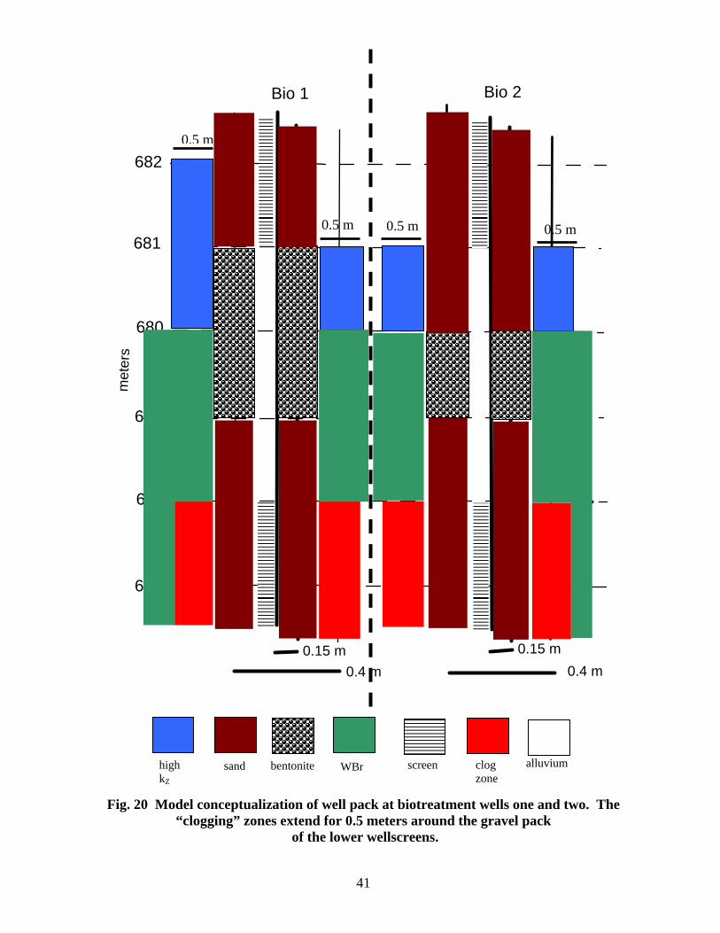
To simulate the short-circuiting behavior at the wells, we incorporated an explicit geometric representation of the well pack, as shown in Figure 20. Each of the biotreatment wells is 0.15 meters in diameter. The well boreholes are 0.4 meters in diameter. The wellpack around the casing consists of sand with a seal between the two screens. The seal is made up of varying grades of sand sandwiching a layer of bentonite. The model includes only the high conductivity sand and the low conductivity bentonite. In order for short-circuiting to occur, water must flow around (or through cracks in) the bentonite seal. In the model we allow this to happen by changing the vertical anisotropy ratio in the material immediately surrounding the bentonite (in a 0.5 meter diameter). Where this surrounding material is the weathered bedrock (which is isotropic), the vertical conductivity is unchanged. However the vertical conductivity of the

11

alluvium is approximately 80 times less than the horizontal conductivity. When the surrounding material is alluvium, the vertical conductivity is significantly increased. The modeled wellpack allows for fast vertical flowpaths from the injection to the pumping wellscreens. The model also includes a clogging zone that extends for 0.5 meters beyond the wellpack at the level of the injection wellscreens. The hydraulic conductivity of the clogging zone is controlled by the CF. Based on transducer readings from the biotreatment wells, we developed a set of five CF parameters, for which values were calibrated, that operate over three clogging periods:

1. December 9, 2001 (day 117) – December 22, 2001 (day 131): Period 1 at Wells 1 and 2 2. December 22, 2001 (day 131)- January 5, 2002 (day 145): Period 2 at Wells 1 and 2 3. January 5, 2002 (day 145) on: Period 3 at Well 2 only

Clogging due to bentonite transport affected the vapor stripping well. When the eductor pipe was pulled from the well, approximately 8 inches of settled bentonite was found sitting on the sealing plate of the pipe. During construction of the vapor stripping well, the bentonite seal was placed 3 feet above the top of the lower sand pack. In retrospect, this was too close to the top of the sand pack, and probably resulted in the bentonite entering the lower screen as a result of settling of the sand pack during well operation. This bentonite clogged the sand pack around the well upper screen, contributing both to a decline in pumping rate and overflow of water. The purpose of the infiltration gallery is to permit water to return freely to the aquifer from the discharge screen of the vapor-stripping well as was done successfully during the previous applications of in-well vapor stripping at Edwards AFB. Care must be taken during construction and operation to ensure that the gallery is not clogged with bentonite. 6.2.6 Tracer Test The bromide tracer test was critical to development of the BEHIVS model. In particular, heterogeneity in the lower aquifer and the variability in effective pumping rates at the biotreatment wells could not have been properly evaluated without the tracer data. Tracer was injected at the vapor stripping well from day 87 through day 92, at an average concentration of 228 mg/L. The tracer injection at bioremediation well one lasted from day 126 though day 132. Over this six-day period the bromide concentration averaged 229 mg/L. The final tracer injection at bioremediation well two started on day 151 and continued through day 160. The average bromide concentration over this time was 237 mg/L. In fact, the concentrations of tracer injected at each well varied over time. Figure 21 shows the bromide concentrations measured at the injection source for each tracer injection. In the model, the concentrations were mass averaged over one-day increments. The bromide concentrations used in the model are shown in Figure 21 as blue bars. The tracer test provided data used to analyze the flow system and to quantify hydraulic parameter values for later use in simulating the BEHIVS process.

12

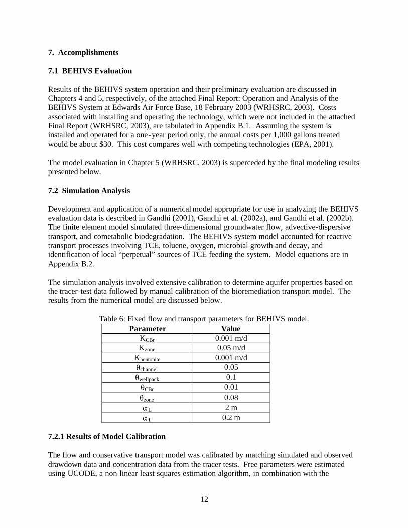
7. Accomplishments 7.1 BEHIVS Evaluation Results of the BEHIVS system operation and their preliminary evaluation are discussed in Chapters 4 and 5, respectively, of the attached Final Report: Operation and Analysis of the BEHIVS System at Edwards Air Force Base, 18 February 2003 (WRHSRC, 2003). Costs associated with installing and operating the technology, which were not included in the attached Final Report (WRHSRC, 2003), are tabulated in Appendix B.1. Assuming the system is installed and operated for a one-year period only, the annual costs per 1,000 gallons treated would be about $30. This cost compares well with competing technologies (EPA, 2001). The model evaluation in Chapter 5 (WRHSRC, 2003) is superceded by the final modeling results presented below. 7.2 Simulation Analysis Development and application of a numerical model appropriate for use in analyzing the BEHIVS evaluation data is described in Gandhi (2001), Gandhi et al. (2002a), and Gandhi et al. (2002b). The finite element model simulated three-dimensional groundwater flow, advective-dispersive transport, and cometabolic biodegradation. The BEHIVS system model accounted for reactive transport processes involving TCE, toluene, oxygen, microbial growth and decay, and identification of local “perpetual” sources of TCE feeding the system. Model equations are in Appendix B.2. The simulation analysis involved extensive calibration to determine aquifer properties based on the tracer-test data followed by manual calibration of the bioremediation transport model. The results from the numerical model are discussed below.

Table 6: Fixed flow and transport parameters for BEHIVS model. Parameter Value

KCBr 0.001 m/d Kzone 0.05 m/d

Kbentonite 0.001 m/d θchannel 0.05 θwellpack 0.1

θCBr 0.01 θzone 0.08 αL 2 m αT 0.2 m

7.2.1 Results of Model Calibration The flow and conservative transport model was calibrated by matching simulated and observed drawdown data and concentration data from the tracer tests. Free parameters were estimated using UCODE, a non- linear least squares estimation algorithm, in combination with the

13

BIOFEM model. The parameters that were calibrated were hydraulic conductivity, vertical anisotropy, effective porosity, and the degree of clogging at the biotreatment wells. Fixed parameters (those not estimated) include dispersivity as well as conductivities and effective porosities in zones insensitive to precise parameter value. These fixed parameter values are given in Table 6. We estimated 13 model parameters using a total of 2,682 data. Of these, 615 were drawdown data comprised of soundings at monitoring wells and transducer readings at treatment wells taken on 13 different days. The first 9 sets of head snapshots represent four sets of pre-clogging pumping conditions:

1. IWVS pumping at 8 gpm and both bioremediation wells at 2 gpm (August 24, September 2, and September 7);

2. IWVS off and both bioremediation wells at 2 gpm (September 19, September 26, October 7, and October 25);

3. IWVS pumping at 7 gpm and both bioremediation wells at 4 gpm (November 14); 4. IWVS pumping at 7 gpm and both bioremediation wells off (September 29); 5. IWVS pumping at 6.8 gpm and both bioremediation wells at 4 gpm (December5).

The remaining three datasets were taken from times after clogging began and were important for estimation of the clogging factors.

6. Clogging period one, day 117-131 (Dec16-21 transducer readings: IWVS pumping at

6.4 gpm and bioremediation wells at 4 gpm); 7. Clogging period two, day 131-145 (January 5: IWVS pumping at 5.2 gpm and

bioremediation wells at 4 gpm); and 8. Clogging period three, after day 145 (January 16: IWVS off and bioremediation wells at

4 gpm). The baseline for calculation of drawdowns was July 27, 2001. Based on two other sets of head data under non-pumping conditions, it was clear that the heads across the site were decreasing over time due to a seasonal decline that has been observed previously at the site. From July 2001 to October 2001, the mean head decrease is 0.07 meters. Similarly, the head decrease from October to February is 0.05 meters. In all three cases the variance is small (on the order of 10-5 meters.) This change was taken into account when calculating modeled drawdowns. The tracer data include a total of 1,026 bromide measurements taken over 52 well locations. Bromide monitoring continued from the start of the tracer test until February 27, 2002. Each data point was weighted equally in the estimation (variance equal to one), however the bromide data were scaled down by 100 so that the residuals would be of the same order of magnitude as the drawdown residuals. The calibrated flow and transport parameter values, as well as the 95% linear confidence intervals, are shown in Table 7.

14

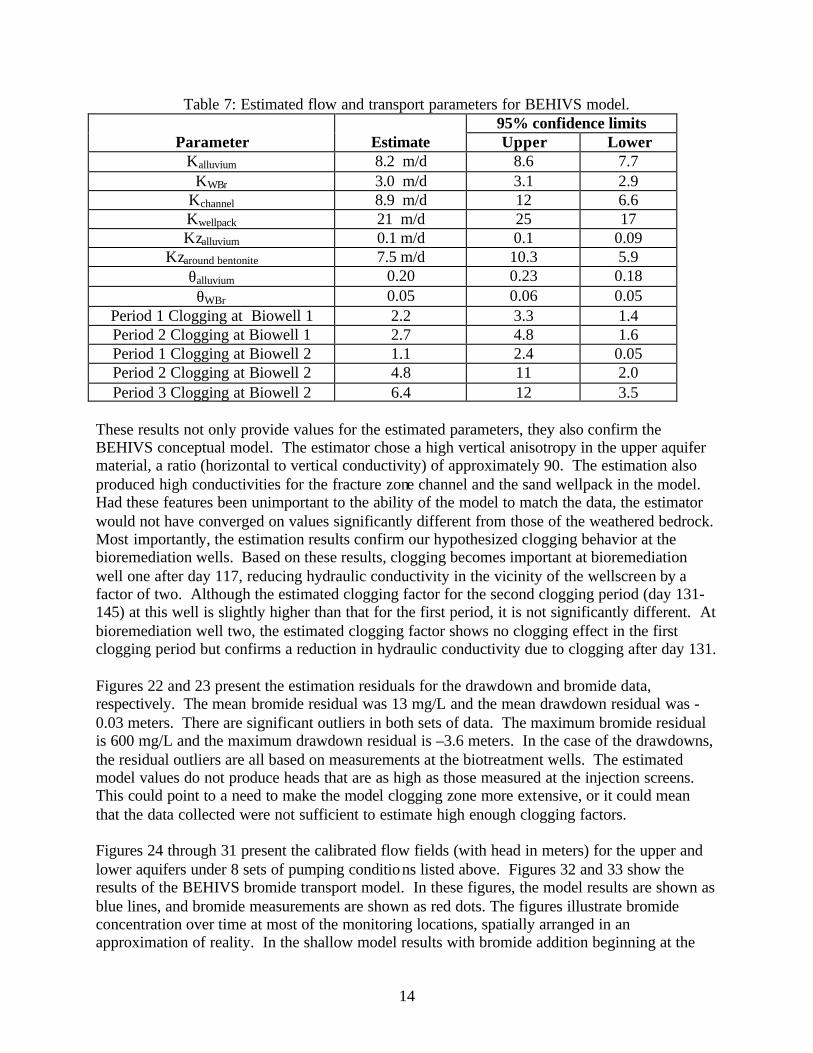
Table 7: Estimated flow and transport parameters for BEHIVS model. 95% confidence limits

Parameter

Estimate Upper Lower Kalluvium 8.2 m/d 8.6 7.7

KWBr 3.0 m/d 3.1 2.9 Kchannel 8.9 m/d 12 6.6 Kwellpack 21 m/d 25 17 Kzalluvium 0.1 m/d 0.1 0.09

Kzaround bentonite 7.5 m/d 10.3 5.9 θalluvium 0.20 0.23 0.18 θWBr 0.05 0.06 0.05

Period 1 Clogging at Biowell 1 2.2 3.3 1.4 Period 2 Clogging at Biowell 1 2.7 4.8 1.6 Period 1 Clogging at Biowell 2 1.1 2.4 0.05 Period 2 Clogging at Biowell 2 4.8 11 2.0 Period 3 Clogging at Biowell 2 6.4 12 3.5

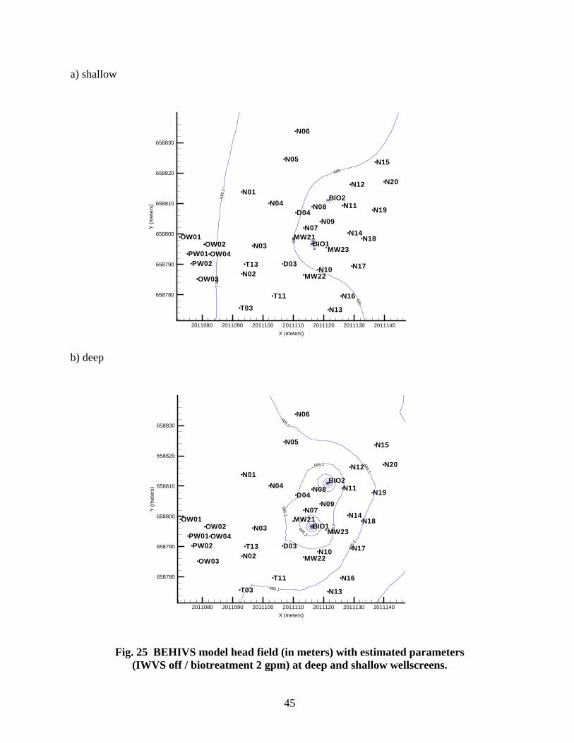
These results not only provide values for the estimated parameters, they also confirm the BEHIVS conceptual model. The estimator chose a high vertical anisotropy in the upper aquifer material, a ratio (horizontal to vertical conductivity) of approximately 90. The estimation also produced high conductivities for the fracture zone channel and the sand wellpack in the model. Had these features been unimportant to the ability of the model to match the data, the estimator would not have converged on values significantly different from those of the weathered bedrock. Most importantly, the estimation results confirm our hypothesized clogging behavior at the bioremediation wells. Based on these results, clogging becomes important at bioremediation well one after day 117, reducing hydraulic conductivity in the vicinity of the wellscreen by a factor of two. Although the estimated clogging factor for the second clogging period (day 131-145) at this well is slightly higher than that for the first period, it is not significantly different. At bioremediation well two, the estimated clogging factor shows no clogging effect in the first clogging period but confirms a reduction in hydraulic conductivity due to clogging after day 131. Figures 22 and 23 present the estimation residuals for the drawdown and bromide data, respectively. The mean bromide residual was 13 mg/L and the mean drawdown residual was -0.03 meters. There are significant outliers in both sets of data. The maximum bromide residual is 600 mg/L and the maximum drawdown residual is –3.6 meters. In the case of the drawdowns, the residual outliers are all based on measurements at the biotreatment wells. The estimated model values do not produce heads that are as high as those measured at the injection screens. This could point to a need to make the model clogging zone more extensive, or it could mean that the data collected were not sufficient to estimate high enough clogging factors. Figures 24 through 31 present the calibrated flow fields (with head in meters) for the upper and lower aquifers under 8 sets of pumping conditions listed above. Figures 32 and 33 show the results of the BEHIVS bromide transport model. In these figures, the model results are shown as blue lines, and bromide measurements are shown as red dots. The figures illustrate bromide concentration over time at most of the monitoring locations, spatially arranged in an approximation of reality. In the shallow model results with bromide addition beginning at the

15

vapor stripping well from day 87 through day 92 (Figure 32), the model fit to the data is quite good at early times, with the exception of the large tracer peak at biotreatment well 2 (solute coming from the vapor stripping well). The model predicts the timing of this peak correctly, thus this quick arrival time suggests some sort of high conductivity feature in the upper alluvium material. The current model did not attempt to create such features in the upper zone. Likewise the modeled peak at MW21 is less than that measured, but the discrepancy is less. Note the second bromide peaks at both of the biotreatment wells. These occur at the same time as the bromide injection at biotreatment well 1 from day 126 though day 132 into the deep aquifer. The model replicates this short-circuiting behavior quite well. The lower aquifer results (Figure 33) also show a quite reasonable match of the model to bromide data. The only peak that the model misses is the biotreatment well 1 bromide peak from the first tracer injection. This is the same peak that the model does not predict in the shallow zone. It is also seen at N11 as it moves downgradient from the biotreatment well. For the most part, the locations where the model fit to the data is the worst are all in the low conductivity zone (N04, N12, MW21). The model is extremely sensitive to the geometry of this zone. The tracer test simulation matches the pattern of tracer arrival from the bromide measurements taken from December through February (days 109 through 198). Both simulation results and the data show that no significant tracer is seen at downgradient wells N13, N15, N16, N17, N19, or N20, nor at upgradient deep wellscreens at N01, N02, N03 or N06. Furthermore, bromide from the tracer injection at bioremediation well one does not appear in significant concentration at any monitoring wells north of the vapor stripper. This is less surprising than the fact that little of the early vapor stripping tracer injection shows up at deep wells N09, N14, and N18, which lie between the two bioremediation wells. These wells only register the later tracer injection at bioremediation well two. This somewhat unintuitive behavior is captured in the model. Table 8 shows a comparison of tracer peak arrival times (days after the peak appears) with modeled peak arrival times. The comparison of the model data with the measured data is accompanied by the caveat that the measurements at any location may have missed the bromide peak. Likewise, the location of smaller peaks is not necessarily recognizable due to analytical measurement error on the order of 50 mg/L. Nonetheless, the model match to the tracer data is quite reasonable. Despite the asymmetries seen in the tracer data (e.g., the difference in peak arrival times from the vapor stripper to each of the biotreatment wells,) the model predicts the existence of tracer only where it occurs in the measurements. At most locations, the peak arrival time is within a day of that measured. This is within the expected margin of error considering that daily averaging was used in the model. The worst model fits are to the third tracer injection at biotreatment well 2 (days 151 through 160). At the time of this tracer injection, the velocities are much slower since the vapor stripping well is off. Thus travel times are longer in general (e.g., 8 days between biotreatment well 2 and N08), and the discrepancy in model to measured peak is exaggerated. Results are moderately good at all locations except N07 shallow and N12 and N18 deep. Given the overall fit to the data shown in Figures 32 and 33, these mismatches do not appear to be critical.

16

Table 8: Comparison of tracer peak arrival time and modeled peak arrival time. Note blanks indicate no discernable peak.

Tracer Peak Arrival Time: Days After Peak at Source First Injection

(IWVS) Second Injection

(Bio1) Third Injection

(Bio2) Well Model

(days) Measured

(days) Model (days)

Measured (days)

Model (days)

Measured (days)

SHALLOW WELLSCREENS D04 source Source 3 3 2 NA Bio 1 2 4 <1 <1 -- -- Bio 2 2 1 -- -- <1 <1 N07 1 1 2 3 15 -- N08 1 <1 2 3 -- -- N09 1 1 7 11 -- -- N11 8 18 -- -- -- -- N14 9 -- -- -- -- -- MW21 2 2 10 16 -- -- MW23 -- -- -- -- -- --

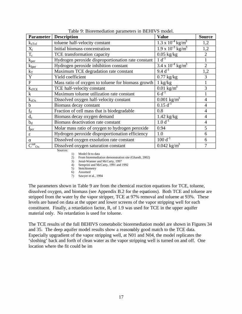
DEEP WELLSCREENS D04 9 5 1 2 11 5 Bio 1 3 2 source source -- -- Bio 2 3 1 -- -- source Source N04 -- -- -- -- 15 10 N05 -- -- -- -- 11 10 N07 3 2 <1 2 -- -- N08 3 1 -- -- 8 10 N09 5 -- -- -- 8 10 N10 7 2 1 2 -- -- N11 3 2 -- -- 8 8 N12 -- -- -- -- 11 37 N14 -- -- -- -- 12 10 N18 -- -- -- -- 33 12 MW21 -- -- 4 2 -- -- MW23 3 16 <1 4 -- -- 7.2.2 TCE Fate and Transport The BEHIVS TCE model includes cometabolic bioremediation processes, removal by in-well vapor stripping, as well as local TCE sources in the BEHIVS treatment area. The TCE sources were hand calibrated using the TCE rebound data collected from February through June 2002. This is discussed further in the next section. The flow and transport parameter values used for the TCE model are taken from the calibrated model discussed in the previous section. Biological parameters for the model were fit by hand or taken from the bioremediation demonstration site (Gandhi et al., 2002b). Table 9 shows the final bioremedation parameters used in the BEHIVS TCE model.

17

Table 9: Bioremediation parameters in BEHIVS model. Parameter Description Value Source ksTol toluene half-velocity constant 1.3 x 10-4 kg/m3 1,2 Xi Initial biomass concentration 1.9 x 10-3 kg/m3 1,2 Tc TCE transformation capacity 0.05 kg/kg 2 kper Hydrogen peroxide disproportionation rate constant 1 d-1 1 kIper Hydrogen peroxide inhibition constant 3.4 x 10-4 kg/m3 2 kT Maximum TCE degradation rate constant 9.4 d-1 1,2 Y Yield coefficient 0.77 kg/kg 3 F Mass ratio of oxygen to toluene for biomass growth 1 kg/kg 1 ksTCE TCE half-velocity constant 0.01 kg/m3 3 k Maximum toluene utilization rate constant 6 d-1 1 ksOx Dissolved oxygen half-velocity constant 0.001 kg/m3 4 b Biomass decay constant 0.15 d-1 4 fd Fraction of cell mass that is biodegradable 0.8 4 dc Biomass decay oxygen demand 1.42 kg/kg 4 bd Biomass deactivation rate constant 1.0 d-1 4 fper Molar mass ratio of oxygen to hydrogen peroxide 0.94 5 ε Hydrogen peroxide disproportionation efficiency 1.0 6 α Dissolved oxygen exsolution rate constant 100 d-1 6 Csat

Ox Dissolved oxygen saturation constant 0.042 kg/m3 7 Sources:

1) Model fit to data 2) From bioremediation demonstration site (Ghandi, 2002) 3) Jenal-Wanner and McCarty, 1997 4) Semprini and McCarty, 1991 and 1992 5) Stoichiometry 6) Assumed 7) Sawyer et al., 1994

The parameters shown in Table 9 are from the chemical reaction equations for TCE, toluene, dissolved oxygen, and biomass (see Appendix B.2 for the equations). Both TCE and toluene are stripped from the water by the vapor stripper, TCE at 97% removal and toluene at 93%. These levels are based on data at the upper and lower screens of the vapor stripping well for each constituent. Finally, a retardation factor, R, of 1.9 was used for TCE in the upper aquifer material only. No retardation is used for toluene. The TCE results of the full BEHIVS cometabolic bioremediation model are shown in Figures 34 and 35. The deep aquifer model results show a reasonably good match to the TCE data. Especially upgradient of the vapor stripping well, at N01 and N04, the model replicates the ‘sloshing’ back and forth of clean water as the vapor stripping well is turned on and off. One location where the fit could be im

18

Figures 36 and 37 show the dissolved oxygen results from the model along with measurements, for deep and shallow wellscreens. Finally Figures 38 and 39 show the toluene fate and transport results for the model. The fit of the model to the measured toluene concentrations is not as good, although this is somewhat expected for two reasons: 1) Toluene measurements were taken once a day while toluene injection occurred for only a fraction of each day—thus the toluene measurements do not accurately represent toluene injection, and 2) The modeled toluene injection is not pulsed as in reality but rather toluene mass is averaged over each day. 7.2.3 Nature of TCE Sources The BEHIVS rebound study (February through June 2002) helped to identify locations for TCE sources in the treatment area—almost all in the deep aquifer. It appears that highly localized hot-spot sources of TCE exist in the bedrock. These local sources are likely to be on the scale of decimeters to a few meters. The dissolved phase TCE in the aquifer is not in equilibrium with these sources that continuously emit solute. The TCE concentrations in the deep zone appear to be controlled by either dissolution of residual TCE, slow diffusion-controlled desorption, or diffusion of a dense highly concentrated dissolved phase that is trapped and immobile. Each of these sources would exhibit similar behavior and cannot be distinguished without further analyses and field investigation. Their locations can be targeted to some degree using the model. Prior to the rebound study, some locations (i.e., N01, N04, N18) on the edge of the treatment area show signs of a TCE source. As the vapor stripping well was turned on and off and the flow direction changed, the TCE concentration in these locations rises and falls. This is especially well illustrated by monitoring well N04. When the vapor stripping well is on, TCE concentrations fall (with a time delay). When the well is off, TCE levels rise again. This behavior was replicated in the BEHIVS model by inserting a continuous fixed concentration TCE source just on the upgradient side of N04. The source was represented by a high concentration extremely low flow (1 liter/day) flux distributed over source nodes. After much exploration of the effects of varying source locations, it was determined that the “sources” of TCE had to be very small (<1 square meter) to achieve the high response behavior seen in the data. If the source covered a larger area, the TCE concentrations are elevated and do not fluctuate with the frequency seen in the data. Other continuous sources appear to be located near the vapor stripping well (D04) and near monitoring well N01. The exact locations and mass fluxes of these sources, based upon model simulations, are given in Appendix B.3, Table 1. The TCE source between well N14 and N18 was found to be better simulated with a rate- limited sorbed source. Similar rate-limited sources appear to be present at N07, N09, N10, Bio1, MW21, and MW22. These sources become apparent from the data in the rebound period, after well operations ceased on day 167. At all of these locations an increase in TCE levels then resulted; at N07 and MW21 TCE concentrations return to pre-BEHIVS levels. The locations and strengths of these sources are shown in Appendix B.3, Table 2. The parameter used to simulate rate- limited TCE sources is not spatially variable, which slightly constrains the ability of the model to fit the data. The desorption rate used for this model was 0.00297 d-1, a value that was fit by trial and error to the rebound concentration data. The locations of TCE sources in the BEHIVS model are shown in Figure 40.

19

7.2.4 Comparison of TCE Treatment Processes Figures 41 and 42 present TCE transport results with no bioactivity, i.e., the biotreatment wells are pumping but no toluene is injected into the system. The purpose of these simulations is to identify the contribution of in-situ degradation using bioremediation on combined BEHIVS treatment results. It is difficult to see much difference between these results and those from the previous two figures. However, the results of bioactivity are pronounced at later times at N05, N07, MW21, and of course the biotreatment wells. When TCE concentrations are low, the biological activity eliminates the tailing seen in the concentrations of Figures 34 and 35. This is consistent with the notion that cometabolic bioremediation is limited to reductions of about 400 µg/L in at this site under these conditions. 7.2.5 Alternate Treatment Scenarios The final model results explore ‘what if’ questions regarding operation of treatment systems at this site. The first scenario involves operating the vapor stripping well only, beginning on August 13, 2001 and running continuously for 320 days. These results are shown in Figures 43 and 44. The expected reduction in TCE concentration is seen throughout the treatment area in the lower aquifer. However, the TCE concentrations remain higher than those seen in the actual BEHIVS operation. This is likely due to the lack of recycling, since only one recirculating well is operating. Without the biotreatment wells pumping in the opposite direction, the contaminated water passes through the vapor stripper once and then leaves the system. Under these operating conditions the spatial area that is affected by the vapor stripping well is larger. So there would be less reduction in TCE concentration, but concentrations would be lowered to some degree over a larger volume. Figures 45 and 46 show the TCE results if all three treatment wells are pumping with vapor stripping occurring at the two (current) biotreatment wells. All three wells are pumping water from the lower aquifer and injecting it into the upper aquifer. TCE levels in the lower aquifer are reduced even further than in the previous scenario due to some of the water undergoing a second pass of the vapor stripper. Again, TCE concentrations remain a little higher than those seen in the actual BEHIVS operation due to lack of recycling. The same scenario as above, where all three treatment wells are pumping with vapor stripping but with the biotreatment wells pumping in the opposite (that is, downflow) direction, is shown in Figures 47 and 48. These results show the great benefits of the recycling system. TCE concentrations at a number of locations (e.g., N08, N07, MW21, N11, MW23, N12, N10, and the biotreatment wells) drop down to near zero. Other locations (N18, N19, N05) see significant reductions in TCE concentrations. Clearly the juxtaposition of recirculating wells pumping in opposite directions is critical to achieving low TCE concentrations.

20

7.3 Publications See Appendix A for a full list of publications. 8. Conclusions 1. Operation of the BEHIVS system resulted in reducing the lower aquifer zone TCE concentrations by 91 percent in the treatment area, with 10 of the 14 monitoring wells showing concentration reductions of between 94 and 97 percent. Average TCE concentrations in the upper aquifer zone within the treatment area were reduced by 56 percent. The total TCE mass removal was 8.1 kg, 7.1 kg of which resulted from in-well vapor stripping and 1.0 kg from biotreatment. 2. TCE concentrations within the BEHIVS study area at Site 19 before the start of the BEHIVS system averaged 4,600 µg/L in the lower portion of the aquifer and 1,240 µg/L in the upper portion of the aquifer. Concentrations in the lower aquifer varied from an average low of 2,480 µg/L at monitoring location N02-L to a high of 8,300 µg/L at monitoring location N04-L. The range in the upper aquifer was 450 µg/L at monitoring location N13-U and a high of 3,000 µg/L at monitoring location N08-U. 3. With a dimensionless air to water ratio between 73 and 90, TCE removal by single-pass vapor stripping averaged between 95 and 97 percent. 4. With an injected toluene concentration of 12 mg/L, maximum percentage removal of TCE through biological treatment was about 70 percent, and the maximum µg/L removal at higher TCE concentrations was about 400 µg/L. Higher percentage removals were obtained with influent TCE concentrations of 400 µg/L or less. At high influent TCE concentrations, percentage removals were less. No more than 400 µg/L TCE could be removed by a single pass through the biotreatment wells. 5. Rebound studies were conducted over a 4 1/2-month period after BEHIVS operation ended. The rebound study indicated that sources of TCE exist in the lower aquifer and are of two types. Both sources, which occur in the fractured bedrock, appear to represent concentrated TCE, ganglia, and/or TCE trapped in small fractures. The first type behaves as a continuous release, which was successfully modeled as a constant flux. This type of source likely represents the constant dissolution and diffusion of TCE from ganglia. The second type behaves as a diffusion-controlled release which was successfully modeled as first-order rate- limited mass transfer from an immobile to an mobile domain. This type of source likely represents the slow diffusion of trapped TCE from fractures or the diffusion from isolated pockets of TCE having high concentrations. At the BEHIVS site rebound brought TCE concentrations up to near the pre-operational level within about 3 1/2 months after BEHIVS operation was stopped. Periodic operation of the BEHIVS system would likely be valuable in preventing high TCE concentrations from migrating down gradient at Site 19.

21

6. Results from field data and the simulation model suggest that clogging in the near-well environment due to microbial growth can reduce the hydraulic conductivity values by up to a factor of three, and thereby change the flow field. Although not catastrophic in terms of system operation, such behavior must be taken into account in order to accurately represent vertical circulation through dual-screened recirculation wells. The relationship between microbial growth and hydraulic properties of aquifer materials is an important research topic as it is poorly understood. 7. The BEHIVS technology proved itself able to cost-effectively treat a TCE-contaminated source zone. Overall, this study shows that the BEHIVS technology has the potential to destroy contaminant mass economically in a NAPL source area without the need to pump contaminated water to the surface for treatment. It was also demonstrated that the complex flow and fate mechanisms occurring in the field could be adequately modeled, and that the model can be used for system design and data analysis. Operational issues, and the relatively short length of the demonstration resulted in a less than fully comprehensive technology evaluation, and more studies are likely needed before the technology can be deployed for commercial application. 9. Transition Plan 1. Preparation of final report to Edwards Air Force Base environmental management personnel and their remediation contractors (accomplished June 2002) 2. Conference presentation of results (for example, at the SERDP-sponsored Partners in Environmental Technology Technical Symposium and Workshop, Washington DC, 3-5 December 2002 and at the AFCEE Technology Transfer Workshop, San Antonio TX, 25-27 February 2003) 3. Publication of demonstration results and model analyses in Water Resources Research (estimated publication date--2004). 4. Presentation to DoD remedial project managers attending Air Force Institute of Technology graduate and professional continuing education courses (ongoing). 5. Operational issues and the relatively short length of the demonstration resulted in a less than fully comprehensive technology evaluation, and more studies are needed before the technology can be fielded for commercial application. These studies can be a continuation of the work at the Edwards AFB site, similar to studies outlined in an earlier proposal to SERDP by the project investigators (McCarty et al., 2001), or longer-term application at a new site, with higher contaminant concentrations. In either case, a model such as that developed as part of the BEHIVS project will be crucial in designing the new studies and interpreting results.

22

10. Recommendations As discussed above, the optimal approach to transition the technology toward commercialization would involve further studies, either at the present Edwards AFB site, or at a new site. The in-well vapor stripping system proved to be simple and effective on its own. The cometabolic bioremediation system was effective but was far more cumbersome and added marginally to the effectiveness of the overall treatment system. As such, it is recommended that future demonstrations employ multiple recirculation wells in critical contaminated regions such as “hot spots” and site boundaries. 11. Report References in Addition to Publications Listed in Appendix A Jenal-Wanner, U. and P.L. McCarty, Development and evaluation of semi-continuous slurry microcosms to simulate in situ biodegradation of trichloroethylene in contaminated aquifers, Environ. Sci. Technol., 31, 2915-2922, 1997. McCarty, P.L., S.M. Gorelick, and M.N. Goltz, Bioenhanced In-Well Vapor Stripping to Treat Trichloroethylene, FY 2002 research proposal submitted to the Strategic Environmental Research and Development Program, 25 July 2001. Sawyer, C.N., P.L. McCarty, and G.F. Parkin, Chemistry for Environmental Engineering, 4th ed., McGraw-Hill, New York, 1994. Semprini, L. and P.L. McCarty, Comparison between model simulations and field results for in-situ biorestoration of chlorinated aliphatics, part 1, Biostimulation of methanotrophic bacteria, Ground Water, 29, 365-374, 1991. Semprini, L. and P.L. McCarty, Comparison between model simulations and field results for in-situ biorestoration of chlorinated aliphatics, part 2, Cometabolic transformations, Ground Water, 30, 365-374, 1992. U.S. Environmental Protection Agency (U.S. EPA), Remediation Technology Cost Compendium—Year 2000, Report EPA-542-R-01-009, Office of Solid Waste and Emergency Response, Washington, DC, September 20.

23

Fig. 1 Section showing BEHIVS concept at Edwards AFB source area.

24

N01

N02

N03

N04

N05

N06

N07

N08

N09

N10

N11

N12

N13

N14

N15

N16

N17

N18

N19

N20

MW21

MW22

MW23BIO1

BIO2

D03

D04

PW01PW02

OW01OW02

OW03

OW04

T03T11

T13

gradient

X (meters)

Y(m

eter

s)

2011070 2011080 2011090 2011100 2011110 2011120 2011130 2011140 2011150

658770

658780

658790

658800

658810

658820

658830

658840

Fig. 2 Monitoring well layout. BEHIVS in-well vapor stripper is D04 and the two biotreatment wells are BIO1 and BIO2.

N

25

Fig. 3 Automated sampling and analysis equipment in analytical trailer

26

N01

N02

N03

N04

N05

N06

N07

N08

N09

N10

N11

N12

N13

N14

N15

N16

N17

N18

N19

N20

MW21

MW22

MW23BIO1

BIO2

D03

D04

PW01PW02

OW01OW02

OW03

OW04

T03T11

T13

gradient

X (meters)

Y(m

eter

s)

2011070 2011080 2011090 2011100 2011110 2011120 2011130 2011140 2011150

658770

658780

658790

658800

658810

658820

658830

658840 Active Treatment

Area

Concentration Reduction 56% Upper 91% Lower

56 meters

48 meters

Fig. 4 Percentage of TCE removal by BEHIVS treatment in the upper and lower portions of the aquifer at Edwards Air Force Base.

27

.

.

Fig. 5 Measured TCE concentrations at vapor stripping well. Note: The difference in concentration between the upper (blue) screen and lower (red) screen is the reduction in

TCE concentration which averaged 95.4%. Note: A logarithmic scale is used for concentrations which are in units of µg/L.

In-Well Vapor Stripping TCE Concentrations

10

100

1000

10000

0 50 100 150 Days

Average Removal 95.4%TCE (µg/L)

28

Fig. 6 Monthly percentage of TCE removal by BEHIVS treatment in the upper and lower portions of the aquifer at Edwards Air Force Base: (A) percent removal in the treatment

zone, and (B) percent removal in the entire monitored zone.

Treatment Zone

0

20

40

60

80

100

Aug

ust

Sept

embe

r

Oct

ober

Nov

embe

r

Dec

embe

r

Janu

ary

Febr

uary

Apr

il

June

Perc

ent R

emov

al

Upper AquiferLower Aquifer

A

Monitored Zone

0

20

40

60

80

100

Aug

ust

Sept

embe

r

Oct

ober

Nov

embe

r

Dec

embe

r

Janu

ary

Febr

uary

Apr

il

June

Perc

ent R

emov

al

Upper AquiferLower Aquifer

B

29

Fig. 7 Mass of TCE removed by vapor stripping well, calculated as the difference between

integrated masses through upper and lower wellscreens.

Fig. 8 Mass of TCE removed by biological treatment.

In-Well Vapor Stripper TCE Mass Removal

0.0

1.0

2.0

3.0

4.0

5.0

6.0

7.0

8.0

0 50 100 150

Days

Tota

l TC

E R

emov

al,

kg

30

a) shallow aquifer

684.96

684.

97

684.97

684.97

684.

9868

4.98

684.

98

684.9 9

684.

99

684.9

9

685

685

685.

0168

5.01

685.0

268

5.02

685.03

685.

03

685.

03

685.04

685.04

685.

0568

5.05

685.05

685.06

685 .

06

685.

06

685.07

685.07

685.

07

685.08

685.

08

685.09

685.0

9

N01

N02

N03

N04

N05

N06

N07

N08

N09

N10

N11

N12

N13

N14

N15

N16

N17

N18

N19

N20

MW21

MW22

MW23BIO1

BIO2

D03

D04

2

OW02

W03

OW04

T03T11

T13

X (meters)

Y(m

eter

s)

2011090 2011100 2011110 2011120 2011130 2011140

658780

658800

658820

b) deep aquifer

684 .96

684.97

684.

97

684.98

684.

98

684.99

684.

99

684.

99

685

685

685

685.01

685.01

685.01

685.02

685.

02

685.0

2

685.03

685.

03

685.03

685.04

685.04

685.0

4

685.05

685.05

685.05

685.

06

685.

06

685.07

685.07

685.

07

685.08

N01

N02

N03

N04

N05

N06

N07

N08

N09

N10

N11

N12

N13

N14

N15

N16

N17

N18

N19

N20

MW21

MW22

MW23BIO1

BIO2

D03

D04

W02

3

OW04

T03T11

T13

x (meters)

y(m

eter

s)

2011090 2011100 2011110 2011120 2011130 2011140 2011150

658780

658800

658820

Fig. 9 BEHIVS site heads measured on July 27, 2001 for shallow (684 meters—top map) and deep (676 meters—bottom map) wellscreens. This map represents flow conditions

prior to BEHIVS system startup; no wells are pumping.

31

N01

N02

N03

N04

N05

N06

N07

N08

N09

N10

N11

N12

N13

N14

N15

N16

N17

N18

N19

N20

MW21

MW22

MW23BIO1

BIO2

D03

D04

PW01PW02

OW01OW02

OW03

OW04

T03T11

T13

X (meters)

Y(m

eter

s)

2011000 2011050 2011100 2011150 2011200

658700

658750

658800

658850

658900

Fig. 10 Plan view of BEHIVS model finite element grid.

IWVS

Bio 2

Bio 1

32

Layers 1, 2, and 3: 685-682 meters

Layer 4: 682-681 meters

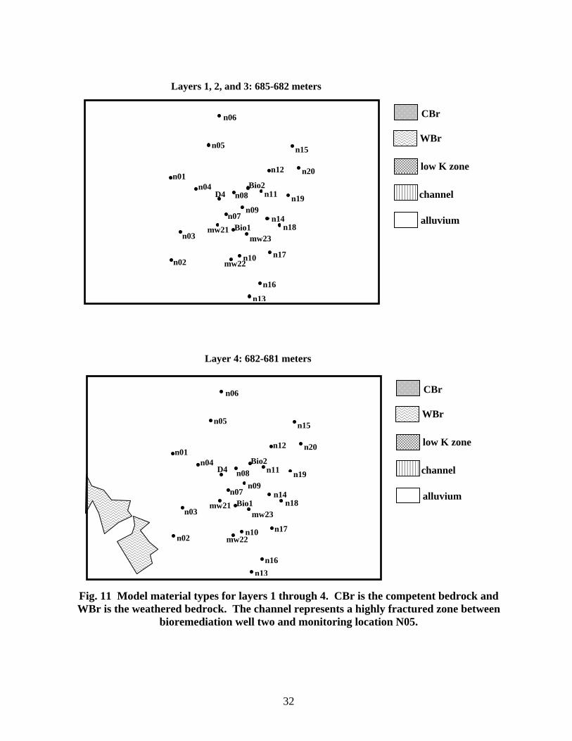
Fig. 11 Model material types for layers 1 through 4. CBr is the competent bedrock and WBr is the weathered bedrock. The channel represents a highly fractured zone between

bioremediation well two and monitoring location N05.

n06

n16

n13

n17

n18

n19

n20

n15

n12

n14

n10mw22 n02

n05

n04 n01

n07 n09

n08D4

Bio1

Bio2

mw21 mw23

n11

n03

CBr

WBr

low K zone

channel

alluvium

n06

n16n13

n17

n18

n19

n20

n15

n12

n14

n10mw22 n02

n05

n04 n01

n07 n09

n08D4

Bio1

Bio2

mw21 mw23

n11

n03

CBr

WBr

low K zone

channel

alluvium

33

Layer 5: 681-680 meters

Layer 6: 680-679 meters Fig. 12 Model material types for layers 5 and 6. CBr is the competent bedrock and WBr is

the weathered bedrock. The channel represents a highly fractured zone between bioremediation well two and monitoring location N05.

n06

n16

n13

n17

n18

n19

n20

n15

n12

n14

n10mw22 n02

n05

n04 n01

n07 n09

n08D4

Bio1

Bio2

mw21 mw23

n11

n03

CBr

WBr

low K zone

channel

alluvium

CBr

WBr

low K zone

channel

alluvium

n06

n16

n13

n17

n18

n19

n20

n15

n12

n14

n10mw22 n02

n05

n04 n01

n07 n09

n08D4

Bio1

Bio2

mw21 mw23

n11

n03

34

Layer 7: 678-679 meters

Layer 8: 677-678 meters

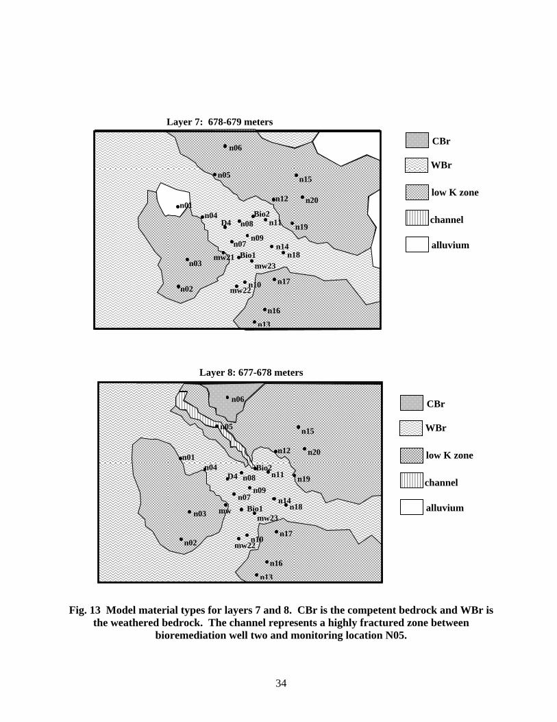
Fig. 13 Model material types for layers 7 and 8. CBr is the competent bedrock and WBr is

the weathered bedrock. The channel represents a highly fractured zone between bioremediation well two and monitoring location N05.

n06

n16

n13

n17

n18

n19

n20

n15

n12

n14

n10 mw22n02

n05

n04 n01

n07n09

n08D4

Bio1

Bio2

mwmw23

n11

n03

CBr

WBr

low K zone

channel

alluvium

n06

n16

n13

n17

n18

n19

n20

n15

n12

n14

n10mw22 n02

n05

n04 n01

n07 n09

n08D4

Bio1

Bio2

mw21 mw23

n11

n03

CBr

WBr

low K zone

channel

alluvium

35

Layer 9: 676-677 meters

Layer 10: 675-676 meters

Fig. 14 Model material types for layers 9 and 10. CBr is the competent bedrock and WBr

is the weathered bedrock. The channel represents a highly fractured zone between bioremediation well two and monitoring location N05.

low K zone

n06

n16

n13

n17

n18

n19

n20

n15

n12

n14

n10mw22 n02

n05

n04 n01

n07 n09

n08D4

Bio1

Bio2

mw21 mw23

n11

n03

CBr

WBr

channel

alluvium

CBr

WBr

low K zone

channel

alluvium

n06

n16

n13

n17

n18

n19

n20

n15

n12

n14

n10mw22 n02

n05

n04 n01

n07 n09

n08D4

Bio1

Bio2

mw21 mw23

n11

n03

36

Layer 11: 673-675 meters

Layers 12 and 13: 665-673 meters

Fig. 15 Model material types for layers 11 through 13. CBr is the competent bedrock and WBr is the weathered bedrock. The channel represents a highly fractured zone between

bioremediation well two and monitoring location N05.

n06

n16

n13

n17

n18

n19

n20

n15

n12

n14

n10mw22 n02

n05

n04 n01

n07 n09

n08D4

Bio1

Bio2

mw21 mw23

n11

n03

CBr

WBr

low K zone

channel

alluvium

CBr

WBr

low K zone

channel

alluvium

n06

n16

n13

n17

n18

n19

n20

n15

n12

n14

n10mw22 n02

n05

n04 n01

n07 n09

n08D4

Bio1

Bio2

mw21 mw23

n11

n03

37

a) shallow aquifer

500

500

1000

1000

1000

1000

1000

1000

1000

1000

1000

1000

1000

1000

1500

15001500

1500

1500

1500

2000N01

N02

N03

N04

N05

N06

N07

N08

N09

N10

N11

N12

N13

N14

N15

N16

N17

N18

N19

N20

MW21

MW22

MW23BIO1

BIO2

D03

D04

2

OW02

W03

OW04

T03T11

T13

X

Y

2.0111E+06 2.01112E+06 2.01114E+06

658780

658790

658800

658810

658820

658830

b) deep aquifer

3000

3000

3000

3000

30003000

35003500

3500

3500 3500

35003500

3500

500

4000

4000

4000

4000

4000

4000

4000

4000

4000

4500

4500

4500

4500

4500

4500

5000

5000

5000

5000

5500

5500

6000

6000

6500N01

N02

N03

N04

N05

N06

N07

N08

N09

N10

N11

N12

N13

N14

N15

N16

N17

N18

N19

N20

MW21

MW22

MW23BIO1

BIO2

D03

D04

2

OW02

W03

OW04

T03T11

T13

X

Y

2.0111E+06 2.01112E+06 2.01114E+06

658780

658790

658800

658810

658820

658830

Fig. 16 Initial TCE concentrations in µg/L for BEHIVS model at upper

(684 meters) and lower (676 meters) locations.

38

a) shallow aquifer

b) deep aquifer

0.5

0.5

0.5

0.5

1.01.0

1.0

1.0

1.0

1.0

1.51.5

1.5

1.5

1.5

1.5

1.5

2.0 2.0

2.0

2.02.0

2.0

2.0

2.5

2.5

2.5

2.5

2.5

2.5

2.5

3.0

3.0

3.0

3.0

3.0

3.0

3.5

3.5

3.5

3.5

4.0

4.0

4.0

4.5

4.5

N01

N02

N03

N04

N05

N06

N07

N08

N09

N10

N11

N12

N14

N15

N16

N17

N18

N19

N20

MW21

MW22

MW23BIO1

BIO2

D03

D04

T11

T13

X (meters)

Y(m

eter

s)

2011100 2011110 2011120 2011130 2011140 2011150

658780

658800

658820

0.0

0.0

0.00.5

0.5

0.5

0.5

0.50.5

0.5

0.5

0.5

1.0

1.0

1.0

1.0

1.0

1.0

1.0

1.0

1.5

N01

N02

N03

N04

N05

N06

N07

N08

N09

N10

N11

N12

N14

N15

N16

N17

N18

N19

N20

MW21

MW22

MW23BIO1

BIO2

D03

D04

T11

T13

X (meters)

Y(m

eter

s)

2011100 2011110 2011120 2011130 2011140 2011150

658780

658800

658820

Fig. 17 Dissolved oxygen initial conditions in mg/L in BEHIVS model in

a) shallow and b) deep aquifers.

39

0 20 40 60 80 100 120 140 160 1800

0.2

0.4

0.6

0.8Return Flow from ASAP

time (days)

Flo

w (

gpm

)

Fig. 18 Sampling return water flow volume. This water is injected into the biotreatment wells until January 9, 2002, at which point it is returned

via the upper screen of the IWVS

40

0 20 40 60 80 100 120 140 160

−1

0

1

2

3

4

5

6

7

8

days since system startup

head

(m

eter

s)

Head Difference in Bio Wells (lower−upper screen)

bio1bio2

Fig. 19 Pressure differential measured from lower to upper screens in biotreatment wells. Clogging periods are defined as 1) day 117-131, 2) day 131-145, and 3)

after day 145.

IWVS off

Double pumping rate at bioremedation wells

IWVS off

Period 1

Period 2

Period 3

41

Bio 1 Bio 2

682

681

680

679

678

677

0.15 m 0.15 m0.4 m 0.4 m

met

ers

Fig. 20 Model conceptualization of well pack at biotreatment wells one and two. The “clogging” zones extend for 0.5 meters around the gravel pack

of the lower wellscreens.

0.5 m

0.5 m

0.5 m 0.5 m

high kZ

sand bentonite WBr screen clog zone

alluvium

42

0 0.5 1 1.5 2 2.5 3 3.5 4 4.5 50

50

100

150

200

250

300

350

400

450

tracer day

brom

ide

ppm

Source Concentration for First Tracer Injection

measurementsmodel

39 40 41 42 43 44 45 460

100

200

300

400

500

600

700

tracer day

brom

ide

ppm

Source Concentration for Second Tracer Injection

measurementsmodel

62 64 66 68 70 72 740

100

200

300

400

500

600

700

800

tracer day

brom

ide

ppm

Source Concentration for Third Tracer Injection

measurementsmodel

Fig. 21 Modeled bromide injection for BEHIVS tracer test. The blue bars are the mass averaged model concentrations (for a one-day time step) and the

red stars are measurements.

43

Fig. 22 Bromide concentration residuals for final estimate results.

Fig. 23 Drawdown residuals for final estimation runs.

44

a) shallow

685 .

1

685.1

685.1

685.2

685.2

685.2

685.

2

685. 3

685.3

685.4

685 .

5

685.5

685.6

685.6

685.

7

686686.

1686.3

686.4

N01

N02

N03

N04

N05

N06

N07

N08

N09

N10

N11

N12

N13

N14

N15

N16

N17

N18

N19

N20

MW21

MW22

MW23BIO1

BIO2

D03

D04

PW01PW02

OW01OW02

OW03

OW04

T03T11

T13

X (meters)

Y(m

eter

s)

2011080 2011090 2011100 2011110 2011120 2011130 2011140

658780

658790

658800

658810

658820

658830

b) deep

684

684.

5

684.6

684.7

684.8

684.8

684.9

684.9

684.9

685

685

685

685

685

685

685.1

685.1

685.3

N01

N02

N03

N04

N05

N06

N07

N08

N09

N10

N11

N12

N13

N14

N15

N16

N17

N18

N19

N20

MW21

MW22

MW23BIO1

BIO2

D03

D04

PW01PW02

OW01OW02

OW03

OW04

T03T11

T13

X (meters)

Y(m

eter

s)

2011080 2011090 2011100 2011110 2011120 2011130 2011140

658780

658790

658800

658810

658820

658830

Fig. 24 BEHIVS model head field (in meters) with estimated parameters (IWVS 7.7 gpm / biotreatment 2.0 gpm) at deep and shallow wellscreens.

45

a) shallow

684.9

685

685

685

685.

1

68 5.1

N01

N02

N03

N04

N05

N06

N07

N08

N09

N10

N11

N12

N13

N14

N15

N16

N17

N18

N19

N20

MW21

MW22

MW23BIO1

BIO2

D03

D04

PW01PW02

OW01OW02

OW03

OW04

T03T11

T13

X (meters)

Y(m

eter

s)

2011080 2011090 2011100 2011110 2011120 2011130 2011140

658780

658790

658800

658810

658820

658830

b) deep

685.1

685.1

685.

1

685.1

685.2

685.

2

685.2

685.3

N01

N02

N03

N04

N05

N06

N07

N08

N09

N10

N11

N12

N13

N14

N15

N16

N17

N18

N19

N20

MW21

MW22

MW23BIO1

BIO2

D03

D04

PW01PW02

OW01OW02

OW03

OW04

T03T11

T13

X (meters)

Y(m

eter

s)

2011080 2011090 2011100 2011110 2011120 2011130 2011140

658780

658790

658800

658810

658820

658830

Fig. 25 BEHIVS model head field (in meters) with estimated parameters (IWVS off / biotreatment 2 gpm) at deep and shallow wellscreens.

46

a) shallow

684.9

685

685

685685.1

685.1

685.

1

685.2

685.2

685.2

685.

3685.

3

6 85.

4

685.4685.5

685.5

685.

6

685.9

686686.2

686.3

N01

N02

N03

N04

N05

N06

N07

N08

N09

N10

N11

N12

N13

N14

N15

N16

N17

N18

N19

N20

MW21

MW22

MW23BIO1

BIO2

D03

D04

PW01PW02

OW01OW02

OW03

OW04

T03T11

T13

X (meters)

Y(m

eter

s)

2011080 2011090 2011100 2011110 2011120 2011130 2011140

658780

658790

658800

658810

658820

658830

b) deep

684.6

684.7

684.

8

684.8684.9

684.9

685

68568

5

685

685.1

685.1

685.1

685.

1

685.

1

685.1

685.2

685.2

685.3

685.4

685.4

685.7

N01

N02

N03

N04

N05

N06

N07

N08

N09

N10

N11

N12

N13

N14

N15

N16

N17

N18

N19

N20

MW21

MW22

MW23BIO1

BIO2

D03

D04

PW01PW02

OW01OW02

OW03

OW04

T03T11

T13

X (meters)

Y(m

eter

s)

2011080 2011090 2011100 2011110 2011120 2011130 2011140

658780

658790

658800

658810

658820

658830

Fig. 26 BEHIVS model head field (in meters) with estimated parameters (IWVS 7 gpm / biotreatment 4 gpm) at deep and shallow wellscreens.

47

a) shallow

685

685.1

685.1

685.1

685.2

685.2

685.2

685.2

685.3

685.3

685.

3

685.4

685.4685.5

685.5

685.6

685.7685.9

686

686.1

686.3

686.4

686.5687.

2

N01

N02

N03

N04

N05

N06

N07

N08

N09

N10

N11

N12

N13

N14

N15

N16

N17

N18

N19

N20

MW21

MW22

MW23BIO1

BIO2

D03

D04

PW01PW02

OW01OW02

OW03

OW04

T03T11

T13

X (meters)

Y(m

eter

s)

2011080 2011090 2011100 2011110 2011120 2011130 2011140

658780

658790

658800

658810

658820

658830

b) deep

684.2

684.3

684.4684. 5

684.6

684.6

684.7

684.7684.8

684.8

684.8

684.9

684.9

684.9

684.9

684.

9

685

685

685

685

685

685.1

685.1

N01

N02

N03

N04

N05

N06

N07

N08

N09

N10

N11

N12

N13

N14

N15

N16

N17

N18

N19

N20

MW21

MW22

MW23BIO1

BIO2

D03

D04

PW01PW02

OW01OW02

OW03

OW04

T03T11

T13

X (meters)

Y(m

eter

s)

2011080 2011090 2011100 2011110 2011120 2011130 2011140

658780

658790

658800

658810

658820

658830

Fig. 27 BEHIVS model head field (in meters) with estimated parameters (IWVS 7.0 gpm / biotreatment wells off ) at deep and shallow wellscreens.

48

a) shallow

684.9

685

685

685.1

685.1

685.

1

685.2

685.2

685.

2685.3

685.3

685.4

685.5

685.

6

685.7 685.

8

686.2

686.4686.5

N01

N02

N03

N04

N05

N06

N07

N08

N09

N10

N11

N12

N13

N14

N15

N16

N17

N18

N19

N20

MW21

MW22

MW23BIO1

BIO2

D03

D04

PW01PW02

OW01OW02

OW03

OW04

T03T11

T13

X (meters)

Y(m

eter

s)

2011080 2011090 2011100 2011110 2011120 2011130 2011140

658780

658790

658800

658810

658820

658830

b) deep

684.6

684.7

684.8

684.9

684.9

685

685

685

685.

1

685.1

685.1

685.1

685.1

685.

1

685.1

685.2

685.

2

685.3

685.4

685.

5

685.5

N01

N02

N03

N04

N05

N06

N07

N08

N09

N10

N11

N12

N13

N14

N15

N16

N17

N18

N19

N20

MW21

MW22

MW23BIO1

BIO2

D03

D04

PW01PW02

OW01OW02

OW03

OW04

T03T11

T13

X (meters)

Y(m

eter

s)

2011080 2011090 2011100 2011110 2011120 2011130 2011140

658780

658790

658800

658810

658820

658830

Fig. 28 BEHIVS model head field (in meters) with estimated parameters (IWVS 6.8 gpm / biotreatment 4 gpm) at deep and shallow wellscreens.

49

a) shallow

685

685

685

685

685.1

685.

1

685.1

685.2

685.2

685.2

685.3685.4685.5685.6

685.8685.9686 68

6.7

N01

N02

N03

N04

N05

N06

N07

N08

N09

N10

N11

N12

N13

N14

N15

N16

N17

N18

N19

N20

MW21

MW22

MW23BIO1

BIO2

D03

D04

PW01PW02

OW01OW02

OW03

OW04

T03T11

T13

X (meters)

Y(m

eter

s)

2011080 2011090 2011100 2011110 2011120 2011130 2011140

658780

658790

658800

658810

658820

658830

b) deep

684.6

684.7

684.

8

684.8

684.9

685

685

685

685.

1

685.1 685.1

685.

1

685.

1

685.1

685.2

685.

2

685.3

685.

3

685.4685.6686.1

N01

N02

N03

N04

N05

N06

N07

N08

N09

N10

N11

N12

N13

N14

N15

N16

N17

N18

N19

N20

MW21

MW22

MW23BIO1

BIO2

D03

D04

PW01PW02

OW01OW02

OW03

OW04

T03T11

T13

X (meters)

Y(m

eter

s)

2011080 2011090 2011100 2011110 2011120 2011130 2011140

658780

658790

658800

658810

658820

658830

Fig. 29 BEHIVS model head field (in meters) with estimated parameters (IWVS 6.8 gpm / biotreatment 4 gpm / clogging period 1) at deep and

shallow wellscreens.

50

a) shallow

684.9

685

685

685

685

685

685.1

685 .1

685.1

685.2

685.2

685.

3

685.4

685.

568

5.6

686.6

N01

N02

N03

N04

N05

N06

N07

N08

N09

N10

N11

N12

N13

N14

N15

N16

N17

N18

N19

N20

MW21

MW22

MW23BIO1

BIO2

D03

D04

PW01PW02

OW01OW02

OW03

OW04

T03T11

T13

X (meters)

Y(m

eter

s)

2011080 2011090 2011100 2011110 2011120 2011130 2011140

658780

658790

658800

658810

658820

658830

b) deep

684.4

684.8

684.

9

685

685

685.

1

685.1

685.1

685.

1

685.1

685.

1

685.1

685.2

685.2

685.

268

5.3

685.3

685.4

685.4

685.5685.7686

N01

N02

N03

N04

N05

N06

N07

N08

N09

N10

N11

N12

N13

N14

N15

N16

N17

N18

N19

N20

MW21

MW22

MW23BIO1

BIO2

D03

D04

PW01PW02

OW01OW02

OW03

OW04

T03T11

T13

X (meters)

Y(m

eter

s)

2011080 2011090 2011100 2011110 2011120 2011130 2011140

658780

658790

658800

658810

658820

658830

Fig. 30 BEHIVS model head field (in meters) with estimated parameters

(IWVS 5.2 gpm / biotreatment 4 gpm / clogging period 2) at deep and shallow wellscreens.

51

a) shallow

684.9

684.9

685

685

685

685.

1

685.

1

N01

N02

N03

N04

N05

N06

N07

N08

N09

N10

N11

N12

N13

N14

N15

N16

N17

N18

N19

N20

MW21

MW22

MW23BIO1

BIO2

D03

D04

PW01PW02

OW01OW02

OW03

OW04

T03T11

T13

X (meters)

Y(m

eter

s)

2011080 2011090 2011100 2011110 2011120 2011130 2011140

658780

658790

658800

658810

658820

658830

b) deep

685.1

685.1

685.1

685.2

685.

2

685.2

685.

2

685.

3

685.

3

685.3

685.4

685.4

685.4

685.5

685.5

685.7

685.

8

685.

9

N01

N02

N03

N04

N05

N06

N07

N08

N09

N10

N11

N12

N13

N14

N15

N16

N17

N18

N19

N20

MW21

MW22

MW23BIO1

BIO2

D03

D04

PW01PW02

OW01OW02

OW03

OW04

T03T11

T13

X (meters)

Y(m

eter

s)

2011080 2011090 2011100 2011110 2011120 2011130 2011140

658780

658790

658800

658810

658820

658830

Fig. 31 BEHIVS model head field (in meters) with estimated parameters

(IWVS off gpm / biotreatment 4 gpm / clogging period 3) at deep and shallow wellscreens.

52

050

100

150

200

250

0

100

200

300

400

500

bio1

s

050

100

150

200

250

0

100

200

300

400

500

bio2

s0

5010

015

020

025

00

100

200

300

400

500

mw

21s

bromide mg/L

050

100

150

200

250

0

100

200

300

400

500

mw

23s

050

100

150

200

250

0

100

200

300

400

500

n01s

050

100

150

200

250

0

100

200

300

400

500

n02s

bromide mg/L

050

100

150

200

250

0

100

200

300

400

500

n03s

050

100

150

200

250

0

100

200

300

400

500

n04s

050

100

150

200

250

0

100

200

300

400

500

n05s

050

100

150

200

250

0

100

200

300

400

500

n06s

050

100

150

200

250

0

100

200

300

400

500

n07s

050

100

150

200

250

0

100

200

300

400

500

n08s

050

100

150

200

250

0

100

200

300

400

500

n09s

050

100

150

200

250

0

100

200

300

400

500

n10s

bromide mg/L

050

100

150

200

250

0

100

200

300

400

500

n11s

050

100

150

200

250

0

100

200

300

400

500

n12s

050

100

150

200

250

0

100

200

300

400

500

n13s

bromide mg/L

050

100

150

200

250

0

100

200

300

400

500

n14s

050

100

150

200

250

0

100

200

300

400

500

n15s

050

100

150

200

250

0

100

200

300

400

500

n16s

bromide mg/L

days

050

100

150

200

250

0

100

200

300

400

500

n17s

days

050

100

150

200

250

0

100

200

300

400

500

n18s

days

050

100

150

200

250

0

100

200

300

400

500

n19s

days

050

100

150

200

250

0

100

200

300

400

500

n20s

days

Tra

cer

Sim

ulat

ion

Res

ults

(bl

ue)

and

Mea

sure

men

ts (

red)

: Sha

llow

Wel

ls

050

100

150

200

250

0

100

200

300

400

500

d04

uppe

r

Fig. 32 BEHIVS model with estimated parameters (blue line) as compared to measured

bromide concentrations (red dots) at shallow wellscreens.

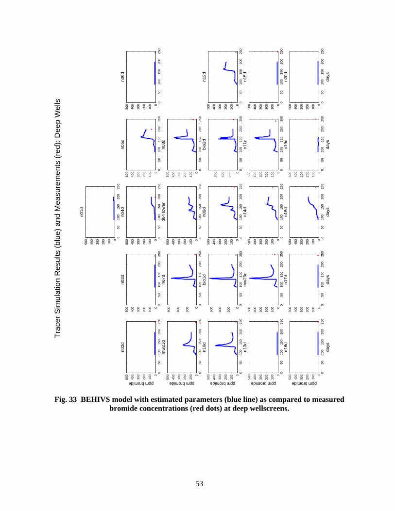
53

050

100

150

200

250

0

200

400

600

bio1

d

050

100

150

200

250

0

200

400

600

bio2

d0

5010

015

020

025

00

100

200

300

400

500

mw

21d

ppm bromide

050

100

150

200

250

0

100

200

300

400

500

mw

23d

050

100

150

200

250

0

100

200

300

400

500

n01d

050

100

150

200

250

0

100

200

300

400

500

n02d

ppm bromide

050

100

150

200

250

0

100

200

300

400

500

n03d

050

100

150

200

250

0

100

200

300

400

500

n04d

050

100

150

200

250

0

100

200

300

400

500

n05d

050

100

150

200

250

0

100

200

300

400

500

n06d

050

100

150

200

250

0

200

400

600

n07d

050

100

150

200

250

0

100

200

300

400

500

n08d

050

100

150

200

250

0

100

200

300

400

500

n09d

050

100

150

200

250

0

100

200

300

400

500

n10d

ppm bromide

050

100

150

200

250

0

100

200

300

400

500

n11d

050

100

150

200

250

0

100

200

300

400

500

n12d

050

100

150

200

250

0

100

200

300

400

500

n13d

ppm bromide

050

100

150

200

250

0

100

200

300

400

500

n14d

050

100

150

200

250

0

100

200

300

400

500

n15d

050

100

150

200

250

0

100

200

300

400

500

n16d

ppm bromide

days

050

100

150

200

250

0

100

200

300

400

500

n17d

days

050

100

150

200

250

0

100

200

300

400

500

n18d

days

050

100

150

200

250

0

100

200

300

400

500

n19d

days

050

100

150

200

250

0

100

200

300

400

500

n20d

days

Tra

cer

Sim

ulat

ion

Res

ults

(bl

ue)

and

Mea

sure

men

ts (

red)

: Dee

p W

ells

050

100

150

200

250

0

100

200

300

400

500

d04

low

er

Fig. 33 BEHIVS model with estimated parameters (blue line) as compared to measured

bromide concentrations (red dots) at deep wellscreens.

54

010

020

030

00

1000

2000

3000

bio1

s

010

020

030

00

1000

2000

3000

bio2

s0

100

200

300

0

1000

2000

3000

mw

21s

TCE µg/L

010

020

030

00

1000

2000

3000

mw

23s

010

020

030

00

1000

2000

3000

n01s

010

020

030

00

1000

2000

3000

n02s

TCE µg/L

010

020

030

00

1000

2000

3000

n03s

010

020

030

00

1000

2000

3000

n04s

010

020

030

00

1000

2000

3000

n05s

010

020

030

00

1000

2000

3000

n06s

010

020

030

00

1000

2000

3000

n07s

010

020

030

00

1000

2000

3000

n08s

010

020

030

00

1000

2000

3000

n09s

010

020

030

00

1000

2000

3000

n10s

TCE µg/L

010

020

030

00

1000

2000

3000

n11s

010

020

030

00

1000

2000

3000

n12s

010

020

030

00

1000

2000

3000

n13s

TCE µg/L

010

020

030

00

1000

2000

3000

n14s

010

020

030

00

1000

2000

3000

n15s

010

020

030

00

1000

2000

3000

n16s

TCE µg/L

days

010

020

030

00

1000

2000

3000

n17s

days

010

020

030

00

1000

2000

3000

n18s

days

010

020

030

00

1000

2000

3000

n19s

days

010

020

030

00

1000

2000

3000

n20s

days

TC

E: S

imul

atio

n R

esul

ts (

blue

) an

d M

easu

rem

ents

(re

d): S

hallo

w W

ells

010

020

030

00

1000

2000

3000

d04

uppe

r

Fig. 34 BEHIVS bioremediation model fit to measured TCE over time at shallow

wellscreens. The blue lines are model results for monitoring well locations and red dots are measurements.

55

010

020

030

00

2000

4000

6000

8000

bio1

d

010

020

030

00

2000

4000

6000

8000

bio2

d0

100

200

300

0

2000

4000

6000

8000

mw

21d

TCE µg/L

010

020

030

00

5000

1000

0

1500

0

mw

23d

010

020

030

00

5000

1000

0

n01d

010

020

030

00

2000

4000

6000

8000

n02d

TCE µg/L

010

020

030

00

2000

4000

6000

8000

n03d

010

020

030

00

5000

1000

0

n04d

010

020

030

00

2000

4000

6000

8000

n05d

010

020

030

00

2000

4000

6000

8000

n06d

010

020

030

00

2000

4000

6000

8000

n07d

010

020

030

00

2000

4000

6000

8000

n08d

010

020

030

00

2000

4000

6000

8000

n09d

010

020

030

00

2000

4000

6000

8000

n10d

TCE µg/L

010

020

030

00

2000

4000

6000

8000

n11d

010

020

030

00

2000

4000

6000

8000

n12d

010

020

030

00

2000

4000

6000

8000

n13d

TCE µg/L

010

020

030

00

2000

4000

6000

8000

n14d

010

020

030

00

2000

4000

6000

8000

n15d

010

020

030

00

2000

4000

6000

8000

n16d

TCE µg/L

days

010

020

030

00

2000

4000

6000

8000

n17d

days

010

020

030

00

2000

4000

6000

8000

n18d

days

010

020

030

00

2000

4000

6000

8000

n19d

days

010

020

030

00

2000

4000

6000

8000

n20d

days

TC

E: S

imul

atio

n R

esul

ts (

blue

) an

d M

easu

rem

ents

(re

d): D

eep

Wel

ls

010

020

030

00

2000

4000

6000

8000

d04

low

er

Fig. 35 BEHIVS bioremediation model fit to measured TCE over time at deep wellscreens.

The blue lines are model results for monitoring well locations and red dots are measurements.

56

010

020

030

005101520

bio1

s

010

020

030

005101520

bio2

s0

100

200

300

05101520m

w21

s

DO mg/L

010

020

030

005101520

mw

23s

010

020

030

005101520

n01s

010

020

030

005101520

n02s

DO mg/L

010

020

030

005101520

n03s

010

020

030

005101520

n04s

010

020

030

005101520

n05s

010

020

030

005101520

n06s

010

020

030

005101520

n07s

010

020

030

005101520

n08s

010

020

030

005101520

n09s

010

020

030

005101520

n10s

DO mg/L

010

020

030

005101520

n11s

010

020

030

005101520

n12s

010

020

030

005101520

n13s

DO mg/L

010

020

030

005101520

n14s

010

020

030

005101520

n15s

010

020

030

005101520

n16s

DO mg/L

days

010

020

030

005101520

n17s

days

010

020

030

005101520

n18s

days

010

020

030

005101520

n19s

days

010

020

030

005101520

n20s

days

DO

: Sim

ulat

ion

Res

ults

(bl

ue)

and

Mea

sure

men

ts (

red)

: Sha

llow

Wel

ls

010

020

030

005101520

d04

uppe

r

Fig. 36 BEHIVS bioremediation model fit to measured dissolved oxygen over time at

shallow wellscreens. The blue lines are model results for monitoring well locations and red dots are measurements.

57

010

020

030

001020

bio1

d

010

020

030

00102030

bio2

d0

100

200

300

05101520

mw

21d

DO mg/L

010

020

030

005101520

mw

23d

010

020

030

005101520

n01d

010

020

030

005101520

n02d

DO mg/L

010

020

030

005101520

n03d

010

020

030

005101520

n04d

010

020

030

005101520

n05d

010

020

030

005101520

n06d

010

020

030

001020

n07d

010

020

030

001020

n08d

010

020

030

005101520

n09d

010

020

030

005101520

n10d

DO mg/L

010

020

030

001020

n11d

010

020

030

005101520

n12d

010

020

030

005101520

n13d

DO mg/L

010

020

030

005101520

n14d

010

020

030

005101520

n15d

010

020

030

005101520

n16d

DO mg/L

days

010

020

030

005101520

n17d

days

010

020

030

005101520

n18d

days

010

020

030

005101520

n19d

days

010

020

030

005101520

n20d

days

DO

: Sim

ulat

ion

Res

ults

(bl

ue)

and

Mea

sure

men

ts (

red)

: Dee

p W

ells

010

020

030

005101520

d04

low

er

Fig. 37 BEHIVS bioremediation model fit to measured dissolved oxygen over time at deep wellscreens. The blue lines are model results for monitoring well locations and red dots are

measurements.

58

010

020

030

00123

x 10

4bi

o1s

010

020

030

0012

x 10

4bi

o2s

010

020

030

00204060

mw

21s

toluene µg/L

010

020

030

0050100

150

200

mw

23s

010

020

030

005101520

n01s

010

020

030

005101520

n02s

toluene µg/L

010

020

030

005101520

n03s

010

020

030

005101520

n04s

010

020

030

005101520

n05s

010

020

030

005101520

n06s

010

020

030

0050100

150

n07s

010

020

030

0010203040

n08s

010

020

030

0020406080

n09s

010

020

030

0050100

n10s

toluene µg/L

010

020

030

00

200

400

600

n11s

010

020

030

0010203040

n12s

010

020

030

005101520

n13s

toluene µg/L

010

020

030

0020406080

n14s

010

020

030

005101520

n15s

010

020

030

00102030

n16s

toluene µg/L

days

010

020

030

0050100

n17s

days

010

020

030

0050100

n18s

days

010

020

030

005101520

n19s

days

010

020

030

005101520

n20s

days

Tol

uene

: Sim

ulat

ion

Res

ults

(bl

ue)

and

Mea

sure

men

ts (

red)

: Sha

llow

Wel

ls

010

020

030

0020406080

d04

uppe

r

Fig. 38 BEHIVS bioremediation model fit to measured toluene over time at shallow

wellscreens. The blue lines are model results for monitoring well locations and red dots are measurements.

59

010

020

030

00246

x 10

4bi

o1d

010

020

030

00510

x 10

4bi

o2d

010

020

030

00

2000

4000

6000

mw

21d

toluene µg/L

010

020

030

00

1000

2000

3000

4000

mw

23d

010

020

030

00

200

400

600

n01d

010

020

030

00204060

n02d

toluene µg/L

010

020

030

0050100

n03d

010

020

030

00

200

400

600

800

n04d

010

020

030

001020

n05d

010

020

030

00

100

200

300

n06d

010

020

030

00123

x 10

4n0

7d

010

020

030

00

2000

4000

6000

8000

n08d

010

020

030

00

500

1000

n09d

010

020

030

00

1000

2000

3000

4000

n10d

toluene µg/L

010

020

030

00

1000

2000

3000

n11d

010

020

030

00

100

200

300

n12d

010

020

030

0020406080

n13d

toluene µg/L

010

020

030

00

500

1000

1500

n14d

010

020

030

00

200

400

600

n15d

010

020

030

002040

n16d

toluene µg/L

days

010

020

030

00102030

n17d

days

010

020

030

00

100

200

300

400

n18d

days

010

020

030

0050100

n19d

days

010

020

030

005101520

n20d

days

Tol

uene

: Sim

ulat

ion

Res

ults

(bl

ue)

and

Mea

sure

men

ts (

red)

: Dee

p W

ells

010

020

030

00

1000

2000

d04

low

er

Fig. 39 BEHIVS bioremediation model fit to measured toluene over time at deep wellscreens. The blue lines are model results for monitoring well locations and

red dots are measurements.

60

N01

N02

N03

N04

N05

N06

N07

N08

N09

N10

N11

N12

N14

N15

N16

N17

N18

N19

N20

MW21

MW22

MW23BIO1

BIO2

D03

D04

T11

T13

X (meters)

Y(m

eter

s)

2011100 2011110 2011120 2011130 2011140 2011150

658780

658800

658820

Fig. 40 Location of TCE continuous sources (yellow circles) and rate-limited rebound sources (blue circles). These sources are very localized, in most cases consisting of two

model nodes.

61

010

020

030

00

1000

2000

3000

bio1

s

010

020

030

00

1000

2000

3000

bio2

s0

100

200

300

0

1000

2000

3000

mw

21s

TCE µg/L

010

020

030

00

1000

2000

3000

mw

23s

010

020

030

00

1000

2000

3000

n01s

010

020

030

00

1000

2000

3000

n02s

TCE µg/L

010

020

030

00

1000

2000

3000

n03s

010

020

030

00

1000

2000

3000

n04s

010

020

030

00

1000

2000

3000

n05s

010

020

030

00

1000

2000

3000

n06s

010

020

030

00

1000

2000

3000

n07s

010

020

030

00

1000

2000

3000

n08s

010

020

030

00

1000

2000

3000

n09s

010

020

030

00

1000

2000

3000

n10s

TCE µg/L

010

020

030

00

1000

2000

3000

n11s

010

020

030

00

1000

2000

3000

n12s

010

020

030

00

1000

2000

3000

n13s

TCE µg/L

010

020

030

00

1000

2000

3000

n14s

010

020

030

00

1000

2000

3000

n15s

010

020

030

00

1000

2000

3000

n16s

TCE µg/L

days

010

020

030

00

1000

2000

3000

n17s

days

010

020

030

00

1000

2000

3000

n18s

days

010

020

030

00

1000

2000

3000

n19s

days

010

020

030

00

1000

2000

3000

n20s

days

TC

E: S

imul

atio

n R

esul

ts (

blue

) an

d M

easu

rem

ents

(re

d): S

hallo

w W

ells

010

020

030

00

1000

2000

3000

d04

uppe

r

Fig. 41 TCE model results with no bioactivity at shallow wellscreens.

62

010

020

030

00

2000

4000

6000

8000

bio1

d

010

020

030

00

2000

4000

6000

8000

bio2

d0

100

200

300

0

2000

4000

6000

8000

mw

21d

TCE µg/L

010

020

030

00

5000

1000

0

1500

0

mw

23d

010

020

030

00

5000

1000

0

n01d

010

020

030

00

2000

4000

6000

8000

n02d

TCE µg/L

010

020

030

00

2000

4000

6000

8000

n03d

010

020

030

00

5000

1000

0

n04d

010

020

030

00

2000

4000

6000

8000

n05d

010

020

030

00

2000

4000

6000

8000

n06d

010

020

030

00

2000

4000

6000

8000

n07d

010

020

030

00

2000

4000

6000

8000

n08d

010

020

030

00

2000

4000

6000

8000

n09d

010

020

030

00

2000

4000

6000

8000

n10d

TCE µg/L

010

020

030

00

2000

4000

6000

8000

n11d

010

020

030

00

2000

4000

6000

8000

n12d

010

020

030

00

2000

4000

6000

8000

n13d

TCE µg/L

010

020

030

00

2000

4000

6000

8000

n14d

010

020

030

00

2000

4000

6000

8000

n15d

010

020

030

00

2000

4000

6000

8000

n16d

TCE µg/L

days

010

020

030

00

2000

4000

6000

8000

n17d

days

010

020

030

00

2000

4000

6000

8000

n18d

days

010

020

030

00

2000

4000

6000

8000

n19d

days

010

020

030

00

2000

4000

6000

8000

n20d

days

TC

E: S

imul

atio

n R

esul

ts (

blue

) an

d M

easu

rem

ents

(re

d): D

eep

Wel

ls

010

020

030

00

2000

4000

6000

8000

d04

low

er

Fig. 42 TCE model results with no bioactivity at deep wellscreens.

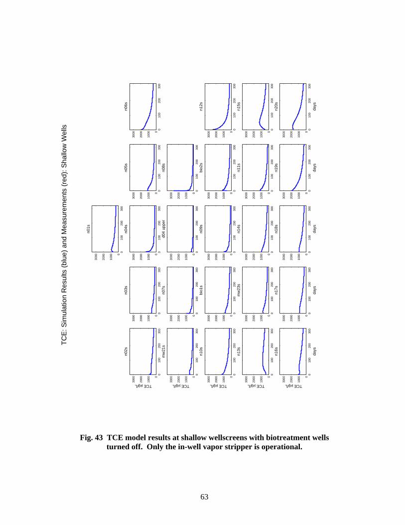
63

010

020

030

00

1000

2000

3000

n01s

010

020

030

00

1000

2000

3000

n02s

TCE µg/L

010

020

030

00

1000

2000

3000

n03s

010

020

030

00

1000

2000

3000

n04s

010

020

030

00

1000

2000

3000

n05s

010

020

030

00

1000

2000

3000

n06s

010

020

030

00

1000

2000

3000

n07s

010

020

030

00

1000

2000

3000

n08s

010

020

030

00

1000

2000

3000

n09s

010

020

030

00

1000

2000

3000

n10s

TCE µg/L

010

020

030

00

1000

2000

3000

n11s

010

020

030

00

1000

2000

3000

n12s

010

020

030

00

1000

2000

3000

n13s

TCE µg/L

010

020

030

00

1000

2000

3000

n14s

010

020

030

00

1000

2000

3000

n15s

010

020

030

00

1000

2000

3000

n16s

TCE µg/L

days

010

020

030

00

1000

2000

3000

n17s

days

010

020

030

00

1000

2000

3000

n18s

days

010

020

030

00

1000

2000

3000

n19s

days

010

020

030

00

1000

2000

3000

n20s

days

010

020

030

00

1000

2000

3000

bio1

s

010

020

030

00

1000

2000

3000

bio2

s0

100

200

300

0

1000

2000

3000

mw

21s

TCE µg/L

010

020

030

00

1000

2000

3000

mw

23s

TC

E: S

imul

atio

n R

esul

ts (

blue

) an

d M

easu

rem

ents

(re

d): S

hallo

w W

ells

010

020

030

00

1000

2000

3000

d04

uppe

r

Fig. 43 TCE model results at shallow wellscreens with biotreatment wells turned off. Only the in-well vapor stripper is operational.

64

010

020

030

00

2000

4000

6000

8000

n01d

010

020

030

00

2000

4000

6000

8000

n02d

TCE µg/L

010

020

030

00

2000

4000

6000

8000

n03d

010

020

030

00

2000

4000

6000

8000

n04d

010

020

030

00

2000

4000

6000

8000

n05d

010

020

030

00

2000

4000

6000

8000

n06d

010

020

030

00

2000

4000

6000

8000

n07d

010

020

030

00

2000

4000

6000

8000

n08d

010

020

030

00

2000

4000

6000

8000

n09d

010

020

030

00

2000

4000

6000

8000

n10d

TCE µg/L

010

020

030

00

2000

4000

6000

8000

n11d

010

020

030

00

2000

4000

6000

8000

n12d

010

020

030

00

2000

4000

6000

8000

n13d

TCE µg/L

010

020

030

00

2000

4000

6000

8000

n14d

010

020

030

00

2000

4000

6000

8000

n15d

010

020

030

00

2000

4000

6000

8000

n16d

TCE µg/L

days

010

020

030

00

2000

4000

6000

8000

n17d

days

010

020

030

00

2000

4000

6000

8000

n18d

days

010

020

030

00

2000

4000

6000

8000

n19d

days

010

020

030

00

2000

4000

6000

8000

n20d

days

010

020

030

00

2000

4000

6000

8000

bio1

d

010

020

030

00

2000

4000

6000

8000

bio2

d0

100

200

300

0

2000

4000

6000

8000

mw

21d

TCE µg/L

010

020

030

00

2000

4000

6000

8000

mw

23d

TC

E: S

imul

atio

n R

esul

ts (

blue

) an

d M

easu

rem

ents

(re

d): D

eep

Wel

ls

010

020

030

00

2000

4000

6000

8000

d04

low

er

Fig. 44 TCE model results at deep wellscreens with biotreatment wells turned off. Only the vapor stripper is operational.

65

010

020

030

00

1000

2000

3000

n01s

010

020

030

00

1000

2000

3000

n02s

TCE µg/L

010

020

030

00

1000

2000

3000

n03s

010

020

030

00

1000

2000

3000

n04s

010

020

030

00

1000

2000

3000

n05s

010

020

030

00

1000

2000

3000

n06s

010

020

030

00

1000

2000

3000

n07s

010

020

030

00

1000

2000

3000

n08s

010

020

030

00

1000

2000

3000

n09s

010

020

030

00

1000

2000

3000

n10s

TCE µg/L

010

020

030

00

1000

2000

3000

n11s

010

020

030

00

1000

2000

3000

n12s

010

020

030

00

1000

2000

3000

n13s

TCE µg/L

010

020

030

00

1000

2000

3000

n14s

010

020

030

00

1000

2000

3000

n15s

010

020

030

00

1000

2000

3000

n16s

TCE µg/L

days

010

020

030

00

1000

2000

3000

n17s

days

010

020

030

00

1000

2000

3000

n18s

days

010

020

030

00

1000

2000

3000

n19s

days

010

020

030

00

1000

2000

3000

n20s

days

010

020

030

00

1000

2000

3000

bio1

s

010

020

030

00

1000

2000

3000

bio2

s0

100

200

300

0

1000

2000

3000

mw

21s

TCE µg/L

010

020

030

00

1000

2000

3000

mw

23s

TC

E: S

imul

atio

n R

esul

ts (

blue

) an

d M

easu

rem

ents

(re

d): S

hallo

w W

ells

010

020

030

00

1000

2000

3000

d04

uppe

r

Fig. 45 TCE model results at shallow wellscreens with all three treatment wells employing

vapor stripping, pumping from lower aquifer and injecting in upper aquifer.

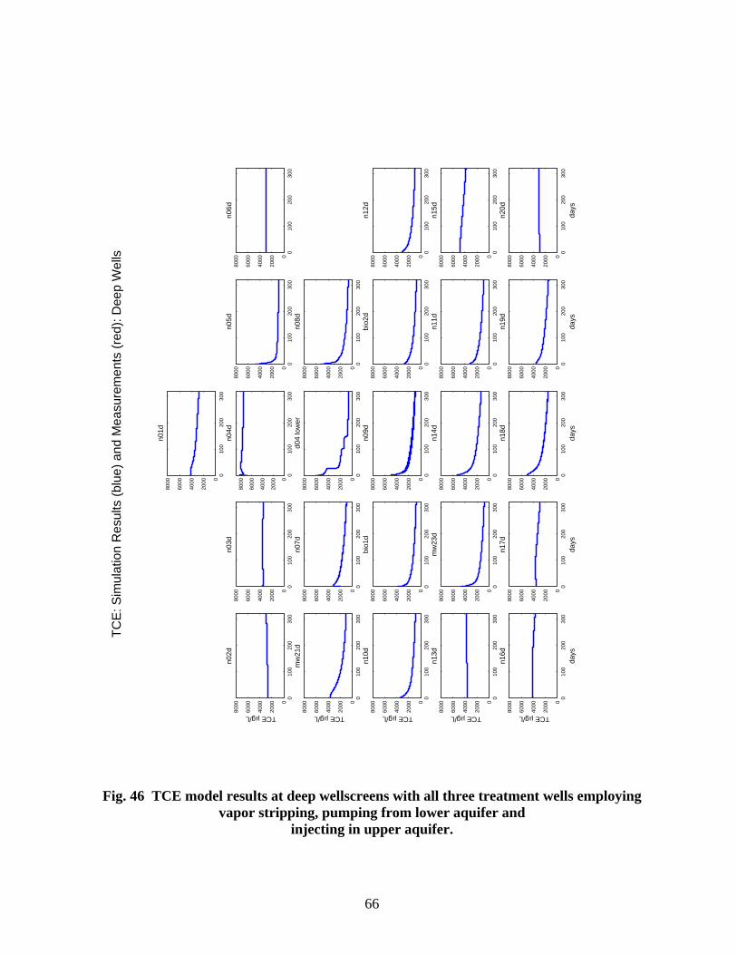
66

010

020

030

00

2000

4000

6000

8000

n01d

010

020

030

00

2000

4000

6000

8000

n02d

TCE µg/L

010

020

030

00

2000

4000

6000

8000

n03d

010

020

030

00

2000

4000

6000

8000

n04d

010

020

030

00

2000

4000

6000

8000

n05d

010

020

030

00

2000

4000

6000

8000

n06d

010

020

030

00

2000

4000

6000

8000

n07d

010

020

030

00

2000

4000

6000

8000

n08d

010

020

030

00

2000

4000

6000

8000

n09d

010

020

030

00

2000

4000

6000

8000

n10d

TCE µg/L

010

020

030

00

2000

4000

6000

8000

n11d

010

020

030

00

2000

4000

6000

8000

n12d

010

020

030

00

2000

4000

6000

8000

n13d

TCE µg/L

010

020

030

00

2000

4000

6000

8000

n14d

010

020

030

00

2000

4000

6000

8000

n15d

010

020

030

00

2000

4000

6000

8000

n16d

TCE µg/L

days

010

020

030

00

2000

4000

6000

8000

n17d

days

010

020

030

00

2000

4000

6000

8000

n18d

days

010

020

030

00

2000

4000

6000

8000

n19d

days

010

020

030

00

2000

4000

6000

8000

n20d

days

010

020

030

00

2000

4000

6000

8000

bio1

d

010

020

030

00

2000

4000

6000

8000

bio2

d0

100

200

300

0

2000

4000

6000

8000

mw

21d

TCE µg/L

010

020

030

00

2000

4000

6000

8000

mw

23d

TC

E: S

imul

atio

n R

esul

ts (

blue

) an

d M

easu

rem

ents

(re

d): D

eep

Wel

ls

010

020

030

00

2000

4000

6000

8000

d04

low

er

Fig. 46 TCE model results at deep wellscreens with all three treatment wells employing

vapor stripping, pumping from lower aquifer and injecting in upper aquifer.

67

010

020

030

00

1000

2000

3000

n01s

010

020

030

00

1000

2000

3000

n02s

TCE µg/L

010

020

030

00

1000

2000

3000

n03s

010

020

030

00

1000

2000

3000

n04s

010

020

030

00

1000

2000

3000

n05s

010

020

030

00

1000

2000

3000

n06s

010

020

030

00

1000

2000

3000

n07s

010

020

030

00

1000

2000

3000

n08s

010

020

030

00

1000

2000

3000

n09s

010

020

030

00

1000

2000

3000

n10s

TCE µg/L

010

020

030

00

1000

2000

3000

n11s

010

020

030

00

1000

2000

3000

n12s

010

020

030

00

1000

2000

3000

n13s

TCE µg/L

010

020

030

00

1000

2000

3000

n14s

010

020

030

00

1000

2000

3000

n15s

010

020

030

00

1000

2000

3000

n16s

TCE µg/L

days

010

020

030

00

1000

2000

3000

n17s

days

010

020

030

00

1000

2000

3000

n18s

days

010

020

030

00

1000

2000

3000

n19s

days

010

020

030

00

1000

2000

3000

n20s

days

010

020

030

00

1000

2000

3000

bio1

s

010

020

030

00

1000

2000

3000

bio2

s0

100

200

300

0

1000

2000

3000

mw

21s

TCE µg/L

010

020

030

00

1000

2000

3000

mw

23s

TC

E: S

imul

atio

n R

esul

ts (

blue

) an

d M

easu

rem

ents

(re

d): S

hallo

w W

ells

010

020

030

00

1000

2000

3000

d04

uppe

r

Fig. 47 TCE model results at shallow wellscreens with all three treatment wells employing vapor stripping, biotreatment well locations are pumping from upper to lower, and vapor-

stripping well is pumping from lower to upper.

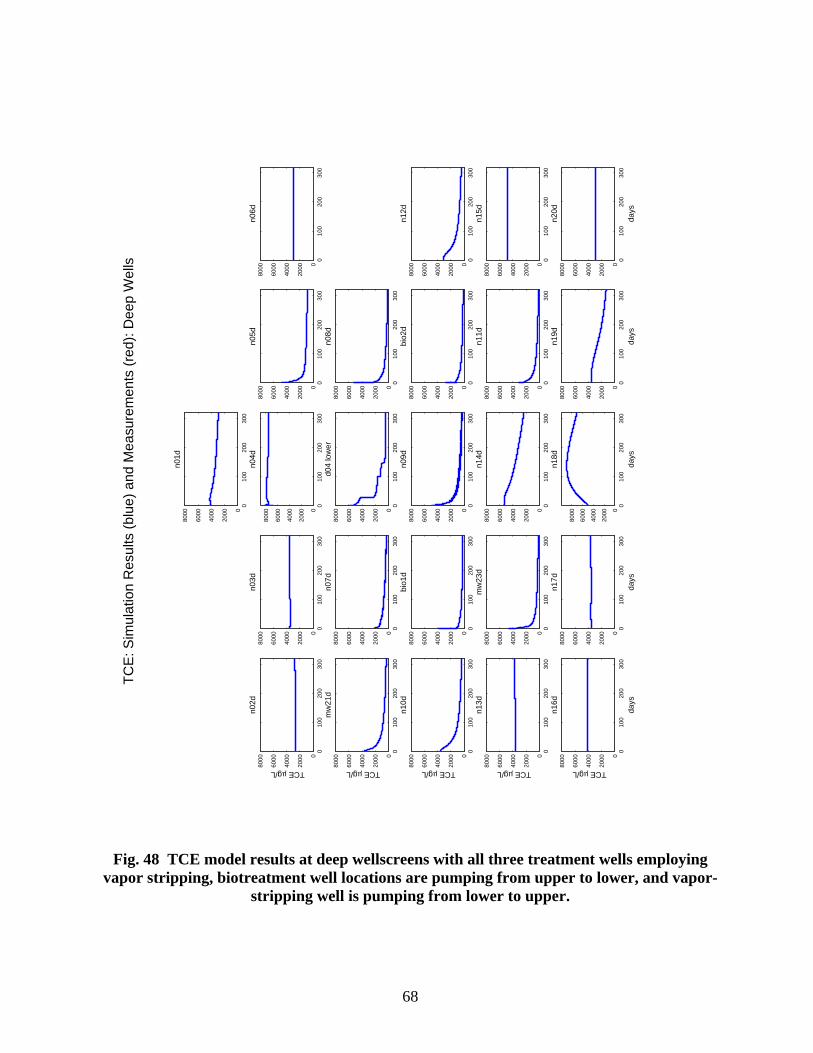
68

010

020

030

00

2000

4000

6000

8000

n01d

010

020

030

00

2000

4000

6000

8000

n02d

TCE µg/L

010

020

030

00

2000

4000

6000

8000

n03d

010

020

030

00

2000

4000

6000

8000

n04d

010

020

030

00

2000

4000

6000

8000

n05d

010

020

030

00

2000

4000

6000

8000

n06d

010

020

030

00

2000

4000

6000

8000

n07d

010

020

030

00

2000

4000

6000

8000

n08d

010

020

030

00

2000

4000

6000

8000

n09d

010

020

030

00

2000

4000

6000

8000

n10d

TCE µg/L

010

020

030

00

2000

4000

6000

8000

n11d

010

020

030

00

2000

4000

6000

8000

n12d

010

020

030

00

2000

4000

6000

8000

n13d

TCE µg/L

010

020

030

00

2000

4000

6000

8000

n14d

010

020

030

00

2000

4000

6000

8000

n15d

010

020

030

00

2000

4000

6000

8000

n16d

TCE µg/L

days

010

020

030

00

2000

4000

6000

8000

n17d

days

010

020

030

00

2000

4000

6000

8000

n18d

days

010

020

030

00

2000

4000

6000

8000

n19d

days

010

020

030

00

2000

4000

6000

8000

n20d

days

010

020

030

00

2000

4000

6000

8000

bio1

d

010

020

030

00

2000

4000

6000

8000

bio2

d0

100

200

300

0

2000

4000

6000

8000

mw

21d

TCE µg/L

010

020

030

00

2000

4000

6000

8000

mw

23d

TC

E: S

imul

atio

n R

esul

ts (

blue

) an

d M

easu

rem

ents

(re

d): D

eep

Wel

ls

010

020

030

00

2000

4000

6000

8000

d04

low

er

Fig. 48 TCE model results at deep wellscreens with all three treatment wells employing

vapor stripping, biotreatment well locations are pumping from upper to lower, and vapor-stripping well is pumping from lower to upper.

69

Appendix A Technical Publications

Peer-reviewed Journal Papers Gandhi, R.K., G.D. Hopkins, M.N. Goltz, S.M. Gorelick, and P.L. McCarty, Full-scale Demonstration of In Situ Cometabolic Biodegradation of Trichloroethylene in Groundwater, 1: Dynamics of a Recirculating Well System, Water Resources Research, 38(4):10.1029/2001WR000379, 2002a. Gandhi, R.K., G.D. Hopkins, M.N. Goltz, S.M. Gorelick, and P.L. McCarty, Full-scale Demonstration of In Situ Cometabolic Biodegradation of Trichloroethylene in Groundwater, 2: Comprehensive Analysis of Field Data Using Reactive Transport Modeling, Water Resources Research, 38(4):10.1029/2001WR000380, 2002b. Technical Reports Gandhi, R.K., Bio-enhanced In-well Vapor Stripping for the Remediation of Trichloroethylene Contamination, Doctoral Dissertation, Stanford University, 2001. Western Region Hazardous Substance Research Center (WRHSRC), Final Report: Operation and Analysis of the BEHIVS System at Edwards Air Force Base, 18 February 2003. Conference/Symposium Proceedings Papers Goltz, M.N., R.K. Gandhi, S.M. Gorelick, G.D. Hopkins, C. LeBron, P.L. McCarty, and M. Reinhard, Application of Circulating Wells for In Situ Treatment of Contaminated Groundwater, Proceedings of International Symposium on Soil and Groundwater Contamination Control Strategy, Kyung Hee University, Seoul, Korea, pp. 3-11, 21 June 2001. Goltz, M.N., R.K. Gandhi, S.M. Gorelick, G.D. Hopkins, and P.L. McCarty, Field Experiments Using In Situ Bioremediation to Treat Trichloroethylene (TCE)-Contaminated Groundwater, Proceeding of the Spring Meeting of the Korean Groundwater and Soil Environment Society, Hanyang University, Seoul, Korea, pp. 261-265, 13-14 April 2001. Published Technical Abstracts McCarty, P.L., S.M. Gorelick, M.N. Goltz, G.D. Hopkins, L.H. Smith, R.K. Gandhi, F-J.Eisenberg, and B. Timmins, Bioenhanced In-Well Vapor Stripping Treatment of TCE Contamination Source, Partners in Environmental Technology Technical Symposium and Workshop, Washington DC, 3-5 December 2002. McCarty, P.L., S.M. Gorelick, M.N. Goltz, G.D. Hopkins, B. Timmins, L. Smith, R.K. Gandhi, and F.-J. Eisenberg, Bioenhanced In-Well Vapor Stripping Treatment of TCE Contamination Source at Edwards Air Force Base, International Groundwater Symposium, Lawrence Berkeley National Laboratory, Berkeley CA, 25-28 March 2002.

70

McCarty, P.L., S.M. Gorelick, M.N. Goltz, G.D. Hopkins, L.H. Smith, R.K. Gandhi, F-J.Eisenberg, and B. Timmins, Bioenhanced In-Well Vapor Stripping of TCE Contamination Source, Partners in Environmental Technology Technical Symposium and Workshop, Washington DC, 27-29 November 2001. Gandhi, R.K., M.N. Goltz, S.M. Gorelick, G.D. Hopkins, and P.L. McCarty, Design of a field demonstration of bio-enhanced in-well vapor stripping to treat trichloroethylene contamination, Hazardous Substance Research Centers Research Symposium, Asilomar Conference Center, CA, 9-12 July 2000. Goltz, M.N., R.K. Gandhi, S.M. Gorelick, G.D. Hopkins, and P.L. McCarty, A Field Demonstration of Bio-enhanced In-Well Vapor Stripping to Treat Trichloroethylene Contamination in Groundwater, Partners in Environmental Technology Technical Symposium and Workshop, Arlington VA, 28-30 November 2000. Agrawal, A., S.R. Maxwell, E.A. Nehring, M.N. Goltz, and P.L. McCarty, Microcosm studies of trichloroethylene cometabolism in support of a field demonstration, In Situ and On-site Bioremediation, San Diego, CA, 19-22 April 1999. Gandhi, R.K., M.N. Goltz, P.L. McCarty, and S.M. Gorelick, Design of a field demonstration of bio-enhanced in-well vapor stripping to treat trichloroethylene contamination, Partners in Environmental Technology Technical Symposium and Workshop, Arlington VA, 30 November - 2 December 1999. Maxwell, S.R., M.N. Goltz, A. Agrawal, and P.L. McCarty, Evaluation of cometabolic biodegradation of trichloroethylene in aerobic slurry microcosms with GRFL (Dover AFB, DE) aquifer material, Gordon Research Conference, Environmental Science-Water, New England College NH, 14-19 June 1998. Goltz, M.N., Bioenhanced in-well vapor stripping to treat trichloroethylene-contaminated groundwater, Western Region Hazardous Substance Research Center Annual Research Symposium, Stanford University CA, 29 July 1998. Goltz, M.N., R. Gandhi, S. R. Maxwell, S. M. Gorelick, A. Agrawal, and P. L. McCarty, Modeling and laboratory studies in support of designing a bioenhanced in-well vapor stripping (BEHIVS) demonstration, Partners in Environmental Technology 98 Technical Symposium and Workshop, Washington DC, 1-3 December 1998. Goltz, M.N., M. Pinto, R. Gandhi, S. M. Gorelick, and P. L. McCarty, Field demonstrations of vertical and horizontal recirculation wells for in situ treatment of chlorinated solvent contaminated groundwater, Partners in Environmental Technology 98 Technical Symposium and Workshop, Washington DC, 1-3 December 1998.

71

Appendix B.1 BEHIVS Costs

CAPITAL COSTS

Biotreatment Well Costs (2 each) 6” Treatment wells $30,000 Flow sensors and controllers $3,000 Static mixers $1,000 Packer assemblies $10,000 Deionized water system $7,000 Pumps and ancillary equipment $10,000 Tubing and connectors $2,000 Valves and fittings $1,000 Total Biotreatment Well Costs $64,000 Vapor Stripping Well Costs Vapor stripping well $30,000 Flow sensors and controllers $6,000 Electric and air conditioning $6,500 Gas regulators, plumbing, mass flow controller $2,000 Hoses, pipes, and fittings $1,000 Granular activated carbon system $10,000 Total Vapor Stripping Well Costs $55,500 TOTAL CAPITAL COSTS $109,500

ANNUAL OPERATING COSTS Hydrogen peroxide $3,000 Toluene (negligible) Carbon dioxide $5,000 Power (@ $0.10 per kwh) $10,000 Granular activated carbon $1,000 ANNUAL OPERATING COST $19,000

72

Appendix B.2 BEHIVS Model Reactive Transport Equations

( )TCETCEdsorpb

OXOX

OX

TCEtol

tolTCE

TCEAT

TCE

CCKK

CKsC

CKsC

Ks

CXFK

dtdC

−−

⎥⎦

⎤⎢⎣

⎡+

⎥⎥⎥⎥⎥

⎦

⎤

⎢⎢⎢⎢⎢

⎣

⎡

+⎟⎟⎠

⎞⎜⎜⎝

⎛+

−=

θρ

1 (B1)

⎥⎦

⎤⎢⎣

⎡+

⎥⎥⎥⎥⎥

⎦

⎤

⎢⎢⎢⎢⎢

⎣

⎡

+⎟⎟⎠

⎞⎜⎜⎝

⎛+⎥

⎥⎦

⎤

⎢⎢⎣

⎡

+−=

OXOX

OX

tolTCE

TCEtol

tol

Iperper

Ipertol

CKsC

CKsC

Ks

CKC

KKX

dtdC

1

(B2)

( )satOXOXperIperper

OXOX

OXdc

OXOX

OX

tolTCE

TCEtol

tol

Iperper

IperOX

CCCKfCKs

CXfbd

CKsC

CKsC

Ks

CKC

KKFX

dtdC

−−+⎥⎦

⎤⎢⎣

⎡+

−

⎥⎦

⎤⎢⎣

⎡+

⎥⎥⎥⎥⎥

⎦

⎤

⎢⎢⎢⎢⎢

⎣

⎡

+⎟⎟⎠

⎞⎜⎜⎝

⎛+⎥

⎥⎦

⎤

⎢⎢⎣

⎡

+−=

αε21

1 (B3)

⎥⎦

⎤⎢⎣

⎡+

⎥⎥⎥⎥⎥

⎦

⎤

⎢⎢⎢⎢⎢

⎣

⎡

+⎟⎟⎠

⎞⎜⎜⎝

⎛+

−⎥⎦

⎤⎢⎣

⎡+

−

⎥⎦

⎤⎢⎣

⎡+

⎥⎥⎥⎥⎥

⎦

⎤

⎢⎢⎢⎢⎢

⎣

⎡

+⎟⎟⎠

⎞⎜⎜⎝

⎛+⎥

⎥⎦

⎤

⎢⎢⎣

⎡

+=

OXOX

OX

TCEtol

tolTCE

TCEAT

OXOX

OX

OXOX

OX

tolTCE

TCEtol

tol

Iperper

Iper

CKsC

CKsC

Ks

CXFK

TcCKsC

bX

CKsC

CKsC

Ks

CKC

KKYX

dtdX

1

1

1 (B4)

73

AdA Fb

dtdF

−= (B5)

perIperper CK

dtdC

−= (B6)

( )TCETCEdsorpTCE CCKK

dtCd

−−= (B7)

Variable Description KsTol toluene half-velocity constant X Biomass concentration Tc TCE transformation capacity Kper Hydrogen peroxide disproportionation rate constant KIper Hydrogen peroxide inhibition constant KT Maximum TCE degradation rate constant Y Yield coefficient F Mass ratio of oxygen to toluene for biomass growth KsTCE TCE half-velocity constant K Maximum toluene utilization rate constant KsOx Dissolved oxygen half-velocity constant B Biomass decay constant fd Fraction of cell mass that is biodegradable dc Biomass decay oxygen demand bd Biomass deactivation rate constant fper Molar mass ratio of oxygen to hydrogen peroxide ε Hydrogen peroxide disproportionation efficiency α Dissolved oxygen exsolution rate constant

satOXC Dissolved oxygen saturation constant

CTCE Dissolved concentration of TCE FA Fraction of active biomass Ctol Dissolved concentration of toluene COX Dissolved oxygen ρb Soil bulk density Ksorp Sorption rate coefficient Kd Soil water partitioning coefficient

TCEC Sorbed concentration of TCE

θ Effective porosity Cper Dissolved peroxide concentration

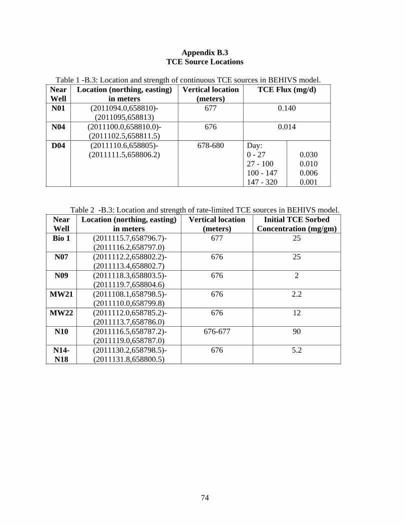
74

Appendix B.3 TCE Source Locations

Table 1 -B.3: Location and strength of continuous TCE sources in BEHIVS model. Near Well

Location (northing, easting) in meters

Vertical location(meters)

TCE Flux (mg/d)

N01 (2011094.0,658810)-(2011095,658813)

677 0.140

N04 (2011100.0,658810.0)-(2011102.5,658811.5)

676 0.014

D04 (2011110.6,658805)-(2011111.5,658806.2)

678-680 Day: 0 - 27 27 - 100 100 - 147 147 - 320

0.030 0.010 0.006 0.001

Table 2 -B.3: Location and strength of rate-limited TCE sources in BEHIVS model. Near Well

Location (northing, easting) in meters

Vertical location (meters)

Initial TCE Sorbed Concentration (mg/gm)

Bio 1 (2011115.7,658796.7)-(2011116.2,658797.0)

677 25

N07 (2011112.2,658802.2)-(2011113.4,658802.7)

676 25

N09 (2011118.3,658803.5)-(2011119.7,658804.6)

676 2

MW21 (2011108.1,658798.5)-(2011110.0,658799.8)

676 2.2

MW22 (2011112.0,658785.2)-(2011113.7,658786.0)

676 12

N10 (2011116.5,658787.2)-(2011119.0,658787.0)

676-677 90

N14- N18

(2011130.2,658798.5)-(2011131.8,658800.5)

676 5.2