Final Report - TU Delft
154
Final Report for the Master’s Thesis Parametric Instability of Deep-Water Risers Student: Joost Brugmans Supervisors: Prof. ir. A.C.W.M. Vrouwenvelder Prof. dr. ir. J.A. Battjes Dr. Sc. A.V. Metrikine Ir. G.L. Kuiper Faculty of Civil Engineering and Geosciences Delft University of Technology Delft, the Netherlands
Transcript of Final Report - TU Delft

Final Report
for the Master’s Thesis
Parametric Instability of Deep-Water Risers
Student: Joost Brugmans Supervisors: Prof. ir. A.C.W.M. Vrouwenvelder Prof. dr. ir. J.A. Battjes Dr. Sc. A.V. Metrikine Ir. G.L. Kuiper Faculty of Civil Engineering and Geosciences Delft University of Technology Delft, the Netherlands

Parametric Instability of Deep-Water Risers
- i -
Preface This document reports the results of my graduation project at the Delft University of Technology. The research is carried out at the section Structural Mechanics of the Faculty of Civil Engineering and Geosciences. The study has been carried out from April 2004 till January 2005. This report is written after several meetings with the graduation committee, who judges the results of this study. The graduation committee consists of the following members: Prof.ir. A.C.W.M. Vrouwenvelder, Prof.dr.ir. J.A. Battjes, Dr.Sc. A.V Metrikine, and ir. G.L. Kuiper. I would like to thank Andrei Metrikine for helping me to understand the mathematical background of this project. He made me aware of mathematical theories which were necessary to do this research. I would like to thank Guido Kuiper for teaching me some common principles in the world of offshore engineering. Their support was an encouragement to accomplish this thesis. I would like to thank professor Battjes for his detailed corrections of my work, not only with respect to the content but also with respect to the writing in English. I would like to thank professor Vrouwenvelder for his contributions during the committee meetings. Delft, January 2005 Joost Brugmans

Parametric Instability of Deep-Water Risers
- ii -

Parametric Instability of Deep-Water Risers
- iii -
Executive Summary During the last decade, some major changes took place in the offshore industry. These changes were associated with new oil and gas fields which were discovered in severe environments, at depths of 1500 meter and more. Nowadays, offshore companies face challenges in the design of risers which could reliably facilitate such deep-water exploration. The heave motion of a floating platform induces a fluctuation in time of the axial tension in the riser. A possible and undesirable phenomenon is the excitation of the lateral response caused by this fluctuation. This phenomenon is called parametric resonance or parametric instability. The objective of this study is to gain better insight in this phenomenon. The focus is on the occurrence of instability for deep-water risers induced by the variation of the effective tension in time. Due to this tension variation the governing equation of motion for the transverse motion of the riser is a partial differential equation containing a time-dependent coefficient. To analyse the stability of the system described by this differential equation three main steps are taken. The normal modes of a closely related system are determined to make it possible to apply the Galerkin’s Method. The normal modes are obtained for the system without the time varying component of the tension force. This equation is a linear partial differential equation of the fourth order whose coefficients are independent of time. To integrate this differential equation a standard FORTRAN routine is used. A study is carried out to find out the features of different methods which are commonly used for analysing the dynamic stability of systems. Three methods are investigated to construct the stability charts of a one-degree of freedom system and a two-degree of freedom system: a small-parameter method, the Floquet theory and the Hill’s method of infinite determinants. For the last two methods programs are written in FORTRAN. A stability chart shows the combinations of magnitude and period of the time varying force for which the system is unstable. The Floquet theory turns out to be the most suitable method to obtain the stability chart of a multiple degree of freedom system including a linear damping term. The Floquet theory is applied to different riser configurations. Not only stability charts are obtained to gain insight in the riser behaviour but also numerically integrations in time are performed for the most critical heave motions of the platform. The results of this analysis are used to estimate the maximum riser displacements. Using these results the bending stresses and additional tensile stresses are calculated. This is done for three riser configurations. Model A is a purely theoretical case: a beam simply supported at both ends with a constant static tension force along the riser. Model B represents the riser system during the drilling operations and production stage: a beam supported at the top by a tensioner system and at the bottom by the sea floor. The static tension is a linear function along the axis. Model C represents the riser during the installation process: a free hanging riser which is fixed to the platform. For this case the static tension is also a linear function along the axis of the tube. Model A is introduced because this system is described by an infinite set of uncoupled differential equations. Model B and Model C are in principal described by a coupled set of differential equations.

Parametric Instability of Deep-Water Risers
- iv -
In this study is shown that the set of differential equations can become decoupled. This is not only the case for the theoretical model but also for the free hanging riser configuration. The reason for this can be found in the small importance of the bending stiffness for very long tubes. In this case the deep-water riser acts like a prestressed cable. The additional condition for the decoupling is the shape of the tension along the riser. The shape of the static tension force and the shape of the additional tension force should be the same. This is true for the free hanging riser. Furthermore, it is shown that the primary instability zones are of much more importance than the secondary instability zones. These secondary zones are very narrow in the stability charts and they move rapidly upwards in the diagram if a damping term (drag force) is introduced in the system. Primary instability occurs for an excitation frequency that equals two times a natural frequency of the system or is a summation of two natural frequencies. This last condition is called combination resonance and is of less importance than the first type, which is called simple resonance. By introducing the drag force in the equation of motion an upper bound of the maximum riser displacement is estimated. Even for the largest expected heave motion the horizontal riser deflection will remain relatively small. This implies that the bending stresses due to this instability problem will not reach alarming values in the ultimate limit state.
KEYWORDS deep-water riser, tensioner system, Galerkin’s method, Floquet theory, linearised drag force

Parametric Instability of Deep-Water Risers
- v -
Table of contents
1. Introduction....................................................................................1 PART A Scope and Objectives of Study 2. Risers in deep water .......................................................................5
2.1 Introduction ....................................................................................................... 5 2.2 Getting oil and gas offshore................................................................................. 5 2.3 Load on the risers............................................................................................... 6 2.4 Analysis of heave motion of floating units ............................................................. 7 2.5 Objective of the study ......................................................................................... 9
3. Riser configurations..................................................................... 11
3.1 Introduction ..................................................................................................... 11 3.2 Governing equation of motion............................................................................ 11 3.3 Model A - simply supported riser with constant tension ........................................ 13 3.4 Model B - fixed riser.......................................................................................... 14 3.5 Model C - free hanging riser .............................................................................. 18
4. Research strategy ........................................................................ 21 PART B Normal Modes of Riser 5. Natural frequencies and normal modes ....................................... 25
5.1 Introduction ..................................................................................................... 25 5.2 Analytical approach: Model A ............................................................................. 25 5.3 Numerical approach: Model B and Model C ......................................................... 31 5.4 Overview ......................................................................................................... 36
PART C Riser Behaviour due to a Parametric Excitation 6. Parametrically excited systems ................................................... 39
6.1 Introduction ..................................................................................................... 39 6.2 Introduction to parametric excitation .................................................................. 39 6.3 Governing system of equations .......................................................................... 40 6.4 Standard form of differential equations containing variable coefficients.................. 46
7. Methods to analyse the dynamic stability.................................... 49
7.1 Introduction ..................................................................................................... 49 7.2 Small parameter method ................................................................................... 49

Parametric Instability of Deep-Water Risers
- vi -
7.3 Floquet theory .................................................................................................. 56 7.4 Hill's method of infinite determinants.................................................................. 61 7.5 Review............................................................................................................. 66
8. Parametric excitation of 1500m risers......................................... 69
8.1 Introduction ..................................................................................................... 69 8.2 Application: simply supported riser with constant tension ..................................... 69 8.3 Application: fixed riser....................................................................................... 80 8.4 Application: free hanging riser ........................................................................... 86
9. Analysis of different riser lengths ................................................ 93
9.1 Introduction ..................................................................................................... 93 9.2 Parametric excitation of 3000m risers ................................................................. 93 9.3 Parametric excitation of 100m water intake risers ................................................ 98
10. Conclusions and recommendations............................................ 103
10.1 Conclusions .....................................................................................................103 10.2 Recommendations ...........................................................................................105
References........................................................................................ 107 Appendix A Riser tension .............................................................................. 111
A-1 General...........................................................................................................111 A-2 Static component.............................................................................................111 A-3 Time varying component of fixed riser ...............................................................113 A-4 Time varying component of free hanging riser....................................................113
B Riser tensioner system............................................................... 115 C Analysis of tension ring in Model B ............................................ 117
C-1 General...........................................................................................................117 C-2 Translation of tension ring ................................................................................118 C-3 Rotation of tension ring....................................................................................121 C-4 Horizontal translation of platform ......................................................................123 C-5 Rotation of platform.........................................................................................124 C-6 Vertical translation of platform ..........................................................................125 C-7 Equation of motion ..........................................................................................125
D Parameters................................................................................. 129

Parametric Instability of Deep-Water Risers
- vii -
E MAPLE sheet for resonance conditions ...................................... 131 E-1 One-degree of freedom system.........................................................................131 E-2 Two-degree of freedom system.........................................................................132
F Analytical expression of the transition curves using the Hill's Determinant ................................................................ 135 G Linearised drag force ................................................................. 139
G-1 General...........................................................................................................139 G-2 Energy method................................................................................................139 G-3 Results for riser configurations..........................................................................141
Error! Bookmark not defined.

Parametric Instability of Deep-Water Risers
- viii -
List of symbols Symbol Definition Unit A amplitude of the heave motion of platform m
sA cross sectional area of the steel wall of the riser m2
b height of tension ring m c linear damping coefficient -
aC added mass coefficient -
dC drag coefficient -
iD inside riser diameter m
oD outside riser diameter m
EI bending stiffness Nm2
f complex amplitude of the external force N/m ( , )f z t external force per unit length acting on the riser N/m
drag( , )f z t drag force acting on riser N/m
mnf coupling factor between mode m and mode n 1/m2
toptenf tensioning factor at riser top -
horF total horizontal force at riser top N
vertF total vertical force at riser top N
g acceleration of gravity m/s2
H hydrostatic head m
zzI moment of inertia m4
ringJ mass moment of inertia of tension ring kgm2
vertk vertical spring coefficient of the riser tensioner system N/m
l width of the tension ring m L length of riser m
horL horizontal projection of the cable length of the tensioner system m
vertL vertical projection of the cable length of the tensioner system m
am added mass per unit length kg/m
fm mass per unit length of the internal fluid kg/m
rm mass per unit length of the riser kg/m
ringM mass of tension ring kg
topM bending moment at riser top Nm
( )M z bending moment in cross section of riser Nm
n integer, defining the number of the mode - N number of degrees of freedom of system - p integer, defining the order of the instability zone -
( )p z hydrostatic pressure N/m2
( )nq t modal coordinate -

Parametric Instability of Deep-Water Risers
- ix -
Symbol Definition Unit
( )S z amplitude of the time varying component of the tension force N
t time s
0T tension force in riser top N
( , )T z t static component of the tension force N
( , )tT z t true riser tension (gravity force minus buoyancy force) N
( )u t horizontal displacement of the tension ring m
plat ( )u t horizontal displacement of the platform m
( , )u z t horizontal water velocity m/s
( , )w z t horizontal displacement of the riser m
z vertical coordinate along the riser m
Greek symbols
nα mode dependent coefficient -
γ angle of the cable of the tension ring with the vertical rad
ε small parameter - ( , )z tζ horizontal velocity of the riser m/s
iλ i th eigenvalue of the state transition matrix -
fρ density of internal fluid kg/m3
sρ steel density kg/m3
wρ seawater density kg/m3
( )b zσ bending stress N/m2
Bσ bending stress criterion N/m2
;addtσ additional tensile stress N/m2
yσ yield stress N/m2
( )tϕ rotation of the tension ring rad
plat ( )tϕ rotation of the platform rad
( )n zφ complex displacement amplitude of n th normal mode m
0( , )t tΦ state transition matrix -
nω natural frequency of n th normal mode rad/s
Ω frequency of the parametric excitation rad/s

Parametric Instability of Deep-Water Risers
- 1 -
1 Introduction During the last decade, some major changes took place in the offshore industry. These changes were associated with new oil and gas fields which were discovered in severe environments, at depths of 1500 meter and more. Nowadays, offshore companies face challenges in the design of risers which could reliably facilitate such deep-water exploration. A riser is a pipe, which connects the wellhead at the seabed to the floating platform. The focus of this thesis project is placed on the transverse displacements of deep-water risers due to the vertical motion of the offshore platform to which the riser top is attached. This platform motion induces a fluctuation in time of the axial tension in the riser. A possible and undesirable phenomenon is the excitation of the lateral response caused by this fluctuation. This phenomenon is called parametric resonance or parametric instability. The possibility of occurrence of this form of dynamic instability is investigated in this report.
Figure 1.1: Semi-Submersible drilling rig This study consists of three main parts (see Figure 1.2): In Part A a short analysis is made to determine to what extent different kind of platforms are vertically excited by incoming waves. Subsequently, the scope and objectives of the study are defined. Furthermore, the general differential equation which describes the transverse motion of a riser is given. This part includes an overview of three riser configurations which are further analysed during this study. Finally, the research strategy to analyse the transverse motion is explained. In Part B the natural frequencies and the corresponding normal modes are determined for the three riser configurations. The time varying tension is neglected in this part. In this case, the

Parametric Instability of Deep-Water Risers
- 2 -
equation of motion is a linear partial differential equation of the fourth order whose coefficients are independent of time. Part C deals with the stability of systems which contain a time dependent coefficient in the governing equation of motion. Three methods are described to construct a stability chart. This chart shows the combinations of magnitude and frequency of this time varying force for which a system is unstable. The most suitable method is applied to the riser configurations to obtain the stability chart for these cases. Figure 1.2: Structure of report
Part A: Scope and Objectives of Study
Ch. 2: Risers in deep water Ch. 3: Riser configurations
Part B: Normal Modes of Riser
Ch. 5: Natural frequencies and normal modes
Part C: Riser Behaviour due to a Parametric Excitation
Ch. 6: Parametrically excited systems Ch. 7: Methods to analyse dynamic stability
Ch. 8: Parametric excitation of 1500m risers Ch. 9: Analysis of different riser lengths
Ch. 10: Conclusions and recommendations
Ch. 4: Research strategy

Parametric Instability of Deep-Water Risers
- 3 -
PART A
Scope and Objectives of Study
Semi-Submersible drilling rig: Ocean Princess

Parametric Instability of Deep-Water Risers
- 4 -

Parametric Instability of Deep-Water Risers
- 5 -
2 Risers in deep water
2.1 Introduction Risers are used in the offshore industry to pump oil or gas from a wellhead at the seabed to a platform. In section 2.2 the successive stages in this process are listed. Section 2.3 contains a short description of the loading mechanisms on the platform-riser system. In section 2.4 an analysis is made to determine for which types of floating units the riser is parametrically excited. The final section contains the objective of this study.
2.2 Getting oil and gas offshore By means of seismic surveys it is possible to detect oil or gas fields. When these geophysical explorations have established that a particular offshore area offers promising prospects, the following three main stages are distinguished:
Stages Offshore unit (in deep water)
1. Drilling operations Semi-Submersible platform, drill ship
2. Installation of production riser Semi-Submersible platform, TLP, SPAR, FPSO
3. Production of gas/oil Semi-Submersible platform, TLP, SPAR, FPSO
Table 2.1: Stages in the exploration and production of oil and gas fields During the production of gas or oil, several types of floating production units can be used, see Table 2.1. In section 2.4 a short description of these platforms or vessels is given. Apart from economics the following aspects are of importance to make the right decision which floating unit will be the best option: the necessity of storage capacity on platform (not available on TLP, limited on SPAR) the need to locate the platform directly above the production well (practical during
maintenance operations) the water depth (tethers of TLP have a maximum allowable tension) the motions of the vessel in waves (operational limits)
For this study it is not necessary to make this decision. It is not even possible because this study is not related to a particular case.

Parametric Instability of Deep-Water Risers
- 6 -
The semi-submersible platform and the drill ship are not connected to the sea bed. In order to enhance the workability, the vertical motions of the platform or ship at the location of the drill string are partly compensated for by a heave compensator. In paragraph 2.4.1 more attention is paid to this device.
2.3 Load on the risers The platform-riser system is loaded by a time-independent (in a short-term view) current and by time-dependent, irregular waves. Irregular waves can be regarded as the result of the summation of an infinite number of sinusoidal waves with random phase. These waves are described by the linear wave theory. Regarding the time-dependent loading mechanisms, the following is noted. A wave that approaches the platform-riser system imposes direct wave loading on the riser. Furthermore, the wave excites the platform, which in turn excites the riser top. These two main mechanisms are shown in Figure 2.1. For a two-dimensional model (only in-plane motions) this incoming harmonic wave results in four loading mechanisms on the riser. All loading mechanisms can be expressed as functions of the incoming wave. Figure 2.1: Loading Mechanisms on the riser due to a regular wave From the mathematical standpoint time-dependent excitations (actions) on a system can be divided in two classes of excitations: - forced or external excitation
The excitation appears as an inhomogeneity in the governing equation of motion. - parametric excitation
The excitation appears as a coefficient in the governing equation of motion. This leads to a differential equation with a time-varying coefficient.
The horizontal and angular excitation of the riser top and the direct wave loading on the riser are forced excitations for the lateral motion of the riser. On the other hand, the vertical excitation of the riser top is a parametric excitation for this motion. The riser tension, which is a coefficient in the governing equation of lateral motion, becomes time-dependent. In contrast with the case of
harmonic wave
platform motions
horizontal excitation of the riser suspension point
vertical excitation of the riser suspension point
angular excitation of the riser suspension point
direct wave loading on riser
riser top excitation

Parametric Instability of Deep-Water Risers
- 7 -
Time
Hor
izon
tal d
ispl
acem
ent
Time
Hor
izon
tal d
ispl
acem
ent
forced excitations in which a small excitation cannot produce large responses unless the frequency of the excitation is close to one of the natural frequencies of the system, a small parametric excitation can produce a large response even when the frequency of the excitation is away from a natural frequency. This phenomenon is called parametric resonance. The word resonance is a misleading term because in reality the structure behaves unstable. The difference between resonance and instability is that the vibration grows linearly in time in case of resonance and exponentially in case of instability. See Figure 2.2a and Figure 2.2b. Figure 2.2a: Instability Figure 2.2b: Resonance
2.4 Analysis of heave motion of floating units In this section an analysis is made to determine for which types of floating units waves can cause instability of the riser. This question is in turn resolved by determining whether the incoming waves cause a heave (vertical) motion of the vessel or platform. Heave of the vessel or platform is a condition for the riser tension to become time-dependent.
2.4.1 Semi-submersible platform For the semi-submersible platform a distinction is made between the different stages since this floating unit can be used in all three stages; see Table 2.1. Drilling operation (including drill ship) During the drilling operation, the drill string is located in a marine riser. The connection of the riser to the semi-submersible platform or drill ship is a tensioned connection. The function of the tensioner system is to support the riser, to maintain the required tension in the riser and to compensate for the relative vertical motion of the riser and the vessel. The compensation of the vertical motion prevents major tensile and compressive stresses in the riser. Figure 2.3 shows a typical tensioner system. This tensioner system consists essentially of soft springs. In this way, the riser can be maintained under the required average tension, while the vertical motions of the vessel do not result in unduly high tension variations. The tensioner system generally applies a tension that is a factor 1.3 larger than the total submerged weight of the riser.

Parametric Instability of Deep-Water Risers
- 8 -
Figure 2.3: Riser tensioner system It is not possible to construct the springs very soft because of technical limits to the design of this device. If the springs are stiff the tension variation in time could be sufficiently large to cause parametric resonance. Thus, during the drilling operation instability of the riser could be an issue because of the heave motion of the semi-submersible platform or drill ship. Installation of production riser During the installation process the configuration comprises a riser that is suspended from the semi-submersible platform and hangs freely downwards by its submerged weight. In this stage it is essential to know the displacements of the riser tip. When the displacements are too large it is very difficult to connect the riser to the well head. The connection of the riser at the top is a fixed connection. This implies that the riser top motions coincide entirely with the platform motions. The vertical motion of the semi-submersible platform invokes an acceleration of the ‘dry’ riser mass. This can be interpreted as an additional gravity force acting on the riser. This causes a fluctuating component of the effective tension in the riser. This could lead to parametric resonance, possibly causing large displacements of the riser, especially of the riser tip. Production of gas/oil The excitation and the configuration of the production riser are equal to the excitation and configuration of the riser during the drilling operation. Thus, for this case the research focuses on the same issue as mentioned above in the part of the drilling operation.
2.4.2 TLP Tension leg platforms are a class of floating structures that are held in place by vertical mooring lines or tendons, extending downwards from each corner of the structure to anchors embedded in the sea floor. The riser structure itself does not experience an oscillating vertical load because of the vertically fixed position of the TLP by these tendons. However, the tendons are subjected to a varying axial force: in addition to the steady buoyancy load, the tendons experience oscillating vertical loads imposed on the structure by passing ocean waves. Thus, the tendons resemble a string in tension where the tension includes a superposed oscillatory component. This implies that parametric resonance can occur but not related to the production riser but related to the tendons. The dynamic behaviour of the tendons is beyond the scope of this research project.
tensioning system

Parametric Instability of Deep-Water Risers
- 9 -
2.4.3 SPAR This offshore structure is shaped in such a way that the heave motion of the platform is relatively small. The structure consists of a long vertical cylinder which is hardly vertically excited by wave loading. The production riser attached to this offshore unit does not experience an oscillating vertical load which is a requirement to cause parametric resonance.
2.4.4 FPSO A FPSO vessel is not as “fixed” in the vertical direction as the TLP above the well. This implies that top-tensioned risers are not applicable, and hence, curved catenary risers are used. These risers can compensate a vertical motion themselves. When the riser is vertically excited by the heave motion of the vessel, the touch-down point where the riser reaches the seabed will shift. This causes a relatively small time varying tension in the riser.
2.5 Objective of the study From the preceding sections it can be concluded that a parametric excitation of a system might produce large lateral responses. This phenomenon is called parametric instability. A vertically hanging riser, suspended or prestressed, is parametrically excited since the incoming waves cause a heave motion of the platform. The heave motion of the platform causes a time-dependent tension in the suspended riser. This is especially the case for semi-submersibles and drill ships in the three above mentioned stages (drilling, installation and production). The objective of this study reads: “The objective of this study is to gain better insight in the phenomenon called parametric instability. The focus is on the occurrence of instability for deep-water risers induced by the variation of the effective tension in time.” To reach this objective, different methods will be investigated for dealing with the stability of periodic systems. The most suitable method will be applied to the case of deep-water risers. A question which should be investigated is the following: “What is the influence of the tensioner system, modelled as prestressed soft springs, on the occurrence of parametric instability during the drilling operation and the production stage?”

Parametric Instability of Deep-Water Risers
- 10 -

Parametric Instability of Deep-Water Risers
- 11 -
3 Riser configurations
3.1 Introduction Instability, caused by a parametric excitation, might lead to large horizontal deflections of the riser. Thus, the most important degree of freedom of a riser is its horizontal deflection. This can be described by making use of a partial differential equation. In section 3.2 the equation of lateral motion for a riser is given. In this partial differential equation the coefficient associated with the riser tension is time-dependent. In the following sections three riser configurations are listed. Each section contains a description of one of these models followed by the boundary conditions.
3.2 Governing equation of motion The equation of motion which is used in this thesis to study the transverse motion of the riser is valid for a number of assumptions, which are summarized below: - one-dimensional model (only in-plane motions) - the slope and curvature of the riser are small - the riser strain is small - stress-strain relations are linear - no internal fluid flow included - structural damping neglected With these assumptions the transverse motion of the vertical riser is governed by equation [3.1]. In Figure 3.1 the system is shown.
( )4 2
4 2
2 31 4
( , ) ( , ) ( , ) ( , )( , ) ( ) ( , )t s r f aw z t w z t w z t w z tEI T z t A p z m m m f z t
z z z zz t∂ ∂ ∂ ∂ ∂ ∂⎡ ⎤ ⎡ ⎤− − + + + =⎢ ⎥ ⎢ ⎥∂ ∂ ∂ ∂∂ ∂⎣ ⎦ ⎣ ⎦144424443 1444424444314243 14444244443
[3.1] where:
EI bending stiffness [Nm2] ( , )tT z t true riser tension (gravity force minus buoyancy force) [N]
sA cross sectional area of the steel wall of the riser [m2]

Parametric Instability of Deep-Water Risers
- 12 -
( )p z hydrostatic pressure [N/m2]
rm mass per unit length of the riser [kg/m]
fm mass per unit length of the internal fluid [kg/m]
am added mass per unit length [kg/m]
( , )f z t external force per unit length acting on the riser [N/m]
( , )w z t horizontal displacement of the riser [m]
z vertical co-ordinate along the riser [m] t time [s]
Figure 3.1: Sketch of a riser system The mass per unit length of the riser, of the internal fluid and the added mass are expressed as follows:
( )ρ π= −2 214r s o im D D [3.2]
214f f im Dρ π= [3.3]
214a a w om C Dρ π= [3.4]
where: oD outside riser diameter [m]
iD inside riser diameter [m]
sρ steel density [kg/m3]
wρ seawater density [kg/m3]
fρ density of internal fluid [kg/m3]
LH
sea floor
,x w
0z =
z
platform
( , )f z t
, rEI m

Parametric Instability of Deep-Water Risers
- 13 -
aC added mass coefficient [-]
All terms on the left hand side of equation [3.1] are ‘restoring terms’ resisting the external loading on the right hand side of the equation. A short explanation of the terms in the equation of motion given by equation [3.1] is given below: 1. The first term represents the horizontal force due to the bending stiffness of the riser. 2. The second term represents the horizontal force due to the tension in the riser, which is
caused by the weight and the buoyancy of the riser. 3. The third term represents the horizontal force due to the hydrostatic external and internal
pressure acting on the riser. The external and internal pressure invoke a horizontal force due to the slope and due to the curvature of the riser.
4. The fourth term is the horizontal force that is caused by inertia of the riser and surrounding fluid. The motion of the riser through the fluid causes a pressure on the riser wall. This pressure is written in terms of a mass, called the added mass.
For a complete derivation of the differential equation the reader is referred to the Master’s thesis of Verkuylen; reference [1]. The equation of motion, equation [3.1], can be rewritten in a shorter form:
4 2
4 2
( , ) ( , ) ( , )( , ) ( ) ( , )r f aw z t w z t w z tEI T z t m m m f z t
z zz t∂ ∂ ∂ ∂⎡ ⎤− + + + =⎢ ⎥∂ ∂∂ ∂⎣ ⎦
[3.5]
where ( , )T z t is the effective tension [N]
The effective tension consists of two elements: the true riser tension ( , )tT z t and the hydrostatic
pressure acting on the riser ( )sA p z . The expression for the effective tension depends on the
riser configuration. Appendix A presents this for a fixed riser and a free hanging riser.
3.3 Model A - simply supported riser with constant tension
3.3.1 Introduction The equation of motion given in equation [3.5] cannot be solved analytically. This differential equation contains one variable coefficient that depends on z and t , which makes this complex to solve. Therefore a simplified model is introduced to start analysing the transverse motion of the riser, namely a riser with constant tension over the depth. This model can be used to verify the numerical results of the more realistic models given in section 3.4 and 3.5. The differential equation can be simplified by using a constant tension force along the z -axis. For this case the equation of motion reads:
∂ ∂ ∂ ∂⎡ ⎤− + + + =⎢ ⎥∂ ∂∂ ∂⎣ ⎦
4 2
4 2
( , ) ( , ) ( , )( ) ( , )( ) r f aw z t w z t w z tEI m m m f
zt
tT z t
zz [3.6]

Parametric Instability of Deep-Water Risers
- 14 -
Furthermore, it is assumed for simplicity that the riser is pinned at both ends. Thus, Model A is purely a theoretical case. The beam model of this riser configuration is shown in Figure 3.2.
Figure 3.2: Beam model, simply supported riser with constant tension
3.3.2 Boundary conditions The riser model is simplified to a simply supported beam. This corresponds to the following boundary conditions for all time instants t : 1.
== plat0
( , ) ( )z
w z t u t [3.7]
2. =
∂=
∂
2
20
( , ) 0z
w z tz
[3.8]
3. ==( , ) 0
z Lw z t [3.9]
4. =
∂=
∂
2
2
( ) 0z L
w Lz
[3.10]
where plat ( )u t is the horizontal displacement of the platform [m]
3.4 Model B - fixed riser 3.4.1 Introduction During the drilling operation, the drill string is located in a marine riser. The connection of the riser to the semi-submersible platform or drill ship is a tensioned connection. The basic principle of the tensioner system is explained in paragraph 2.4.1. In this section the tensioner system is shown in more detail. This is necessary to obtain the correct schematic representation of this riser configuration. Figure 3.3a shows the basic elements of the tensioner system. The corresponding beam model of the riser is shown in Figure 3.3b.
, EI m L
( , )f z t
platform

Parametric Instability of Deep-Water Risers
- 15 -
Figure 3.3a: Tensioned connection riser-platform Figure 3.3b: Beam model, fixed riser structure Comment on Figure 3.3a and Figure 3.3b Pulleys are connected to the tension ring around the riser top. The pistons provide the tensioning force on the riser. This implies that the two springs shown in Figure 3.3 provide a large static tensile force, the pre-tension. In contrast to Figure 3.2, the pistons are connected to a very large volume on the pressurised side. This implies that vertical displacements of the platform invoke minor tension variation in the riser. Thus, the
spring coefficient k in Figure 3.3 is very small. For more information about this device the reader is referred to Appendix B.
3.4.2 Boundary Conditions Riser top As shown in Figure 3.3a and Figure 3.3b the connection to the platform consists of soft springs. These springs are not attached to the riser itself but to the tension ring. Figure 3.4 shows the schematization of the upper part of the riser in detail. Figure 3.4: Connection at top of fixed riser structure
1
2
3
4
3
4
5
1. Riser
2. Tension Ring
3. Pulley
4. Piston
5. Platform Deck
( , )w z t
platl
z
b
l
ϕu
= 0z
γ
ring ring, M J
platu
ϕplat
platS
, EI m
kk
L
M
platform
( , )f z t

Parametric Instability of Deep-Water Risers
- 16 -
The riser is schematized as a bar with an infinite axial stiffness. That is why the third degree of freedom of the tension ring, the vertical motion, is not shown in Figure 3.4. The riser-tension ring connection can be mathematically described by the following two boundary conditions:
1. ϕ== + ⋅
0( , ) ( ) ( )
2z
bw z t u t t [3.11]
2. ϕ=
∂=
∂ 0
( , ) ( )z
w z t tz
[3.12]
where: ( )u t horizontal displacement of the tension ring [m]
( )tϕ rotation of the tension ring [rad]
b height of the tension ring [m] Two equations of motion are derived for the tension ring; one is obtained for the horizontal motion and one for the rotational motion. See Appendix C for the derivation of equation [3.15] and equation [3.16]. These equations are based upon the following assumptions: - The forces in the cables of the tensioner system consist of two components. A static tension
force which remains constant and an additional tension force which is proportional to the elongation of the cables.
- The change of the angle of the cables with the vertical is small compared to the angle for the situation in which no rotation or translation occurs: γ γ∆ .
- The forces of the slip joint at the top of the tension ring are neglected.
( )2
20 0ring hor plat2
vert vert
plat0plat plat
vert
d ( ) 2 2 sin ( ) ( ) tan sin cos ( )2d
tan sin cos ( )2
T Tu tM F k u t u t k tL Lt
Tk t
L
γ γ γ γ ϕ
γ γ γ ϕ
⎛ ⎞ ⎛ ⎞⋅ = − + ⋅ − + ⋅ − ⋅ ⋅⎜ ⎟ ⎜ ⎟
⎝ ⎠ ⎝ ⎠⎛ ⎞
− ⋅ − ⋅ ⋅⎜ ⎟⎝ ⎠
ll
ll
[3.15]
( )2
0ring top hor plat2
vert
2 22 20 0
vertvert
plat20
vert
d ( ) tan sin cos ( ) ( )2 2d
tan tan cos ( )4 2 2 2
tan4
Tt bJ M F k u t u tLt
T T bk F tL
Tk
L
ϕ γ γ γ
γ γ γ ϕ
γ
⎛ ⎞⋅ = − + + ⋅ − ⋅ ⋅ −⎜ ⎟
⎝ ⎠⎛ ⎞
− ⋅ + ⋅ + ⋅ − ⋅⎜ ⎟⎝ ⎠
− ⋅ ⋅ +
ll
l ll
ll
plat2platcos ( )
2tγ ϕ
⎛ ⎞⋅ ⋅ ⋅⎜ ⎟
⎝ ⎠
ll
[3.16]
where: ringM mass of tension ring [kg]
ringJ mass moment of inertia of tension ring [kgm2]
0T tension force in riser top [N]
l width of the tension ring [m] γ angle of cable with the vertical [rad]

Parametric Instability of Deep-Water Risers
- 17 -
topM
horF vertF
(0, )V t
(0, )M t
(0, )T t
plat ( )u t horizontal displacement of the platform [m]
ϕplat ( )t rotation of the platform [rad]
vertL vertical projection of the cable length of the tensioner system [m]
horF total horizontal force at riser top [N]
vertF total vertical force at riser top [N]
topM bending moment at riser top [Nm]
The expressions for the forces ( horF , vertF ) and the bending moment ( topM ) which are used in
equation [3.15] and equation [3.16] are defined as follows:
=
∂= + ⋅
∂hor0
( , )(0, ) (0, )z
w z tF V t T tz
[3.17]
=
∂= − ⋅
∂vert0
( , )(0, ) (0, )z
w z tF T t V tz
[3.18]
top (0, )M M t= [3.19]
This is derived using the forces on the differential element at 0z = , which is shown in Figure 3.5: Figure 3.5: Internal forces at top section Riser tip The riser structure at the sea bed can be considered as a pinned connection; see Figure 3.3. This provides the following boundary conditions at z L= : 3.
==( , ) 0
z Lw z t [3.20]
4. =
∂=
∂
2
2
( , ) 0z L
w z tz
[3.21]
where:
=
∂= −
∂
2
20
( , )(0, )z
w z tM t EIz
=
∂= −
∂
3
30
( , )(0, )z
w z tV t EIz
= 0(0, )T t T , static tension at the riser top

Parametric Instability of Deep-Water Risers
- 18 -
3.5 Model C - free hanging riser
3.5.1 Introduction When the drilling operations are finished, the production riser is installed. During this installation process the riser configuration concerns a riser that is suspended from the production platform and hangs freely downwards by its submerged weight. This implies that the riser top motions coincide entirely with the platform motions. The corresponding beam model of the riser is shown in Figure 3.6.
Figure 3.6: Beam model, free hanging riser structure
3.5.2 Boundary Conditions Riser top The free hanging riser is fixed to the vessel or platform. This fixation transfers all horizontal, vertical and angular motions of the riser suspension point to the riser top. Thus, the two boundary conditions defined at 0z = are given by: 1.
== plat0
( , ) ( )z
w z t u t [3.22]
2. ϕ=
∂=
∂ plat0
( , ) ( )z
w z t tz
[3.23]
where: plat ( )u t horizontal displacement of the platform [m]
plat ( )tϕ rotation of the platform [rad]
Riser tip At the riser base the total horizontal force and the bending moment should be equal to zero. This provides the following boundary conditions at z L= :
, EI m L
platform
( , )f z t

Parametric Instability of Deep-Water Risers
- 19 -
3. == =
∂ ∂ ∂− + = ⇔ =
∂∂ ∂
3 3
3 3
( , ) ( , ) ( , )( , ) 0 0z Lz L z L
w z t w z t w z tEI T L tzz z
[3.24]
4. = =
∂ ∂− = ⇔ =
∂ ∂
2 2
2 2
( , ) ( , )0 0z L z L
w z t w z tEIz z
[3.25]
The term associated with the effective tension vanishes from the third boundary condition because the effective tension force at z L= is equal to zero:
0 0( , ) ( , ) ( ) ( ) 0 0t s g b s s w s wT L t T L t p L A F F p L A A g H A g Hρ ρ= + ⋅ = − + ⋅ = − + =

Parametric Instability of Deep-Water Risers
- 20 -

Parametric Instability of Deep-Water Risers
- 21 -
4 Research strategy The governing equation of motion with the time-dependent coefficient might predict the parametric instability. The Galerkin Approach is used to find the conditions for this kind of instability. To apply this method we need a closely related system with orthogonal modes. This system can be obtained by neglecting the time varying tension force. This ‘pre-work’ is done in Part B. The resulting equation of motion yields:
∂ ∂ ∂ ∂⎡ ⎤− + + + =⎢ ⎥∂ ∂∂ ∂⎣ ⎦
4 2
4 2( ) ( ,( , )) ( , ) ( , )( )r f aw z t w z t w z tEI mT z fm m
z tz
zt
z [4.1]
This equation is a linear partial differential equation of the fourth order whose coefficients are independent of time. The natural frequencies and the corresponding normal mode shapes are determined for the three riser configurations as explained in Chapter 3. The first model is a simplified model which can be analysed analytically. Model B represents the riser during the drilling operation and production stage (fixed to the sea floor). The third configuration represents the installation stage (free hanging). The natural frequencies are found by applying an external force on the riser ( , )f z t . The excitation frequencies for which the horizontal displacements of the
risers reach a peak value correspond to the natural frequencies of the analysed riser models. This way of calculating the natural frequencies is chosen for its numerical convenience. The results of this part are used in Part C in which the stability charts for the riser configurations are constructed. In part C the time varying tension is included in the equation of motion, see equation [3.5]. It is not necessary to include an external force acting on the riser to analyse the stability of the system. When dealing with linear models a small disturbance in the riser shape is sufficient to determine the properties of the behaviour of the system. Thus, the equation of motion is a homogeneous partial differential equation of the fourth order whose coefficients vary in time; see equation [4.2].
∂ ∂ ∂ ∂⎡ ⎤− + + + =⎢ ⎥∂ ∂∂ ∂⎣ ⎦
4 2
4 2
( , ) ( , ) ( , ) 0( )( , ) r f aw z t w z t w z tEI m m m
z zt
tT z
z [4.2]
The main aim of this part is to construct a stability chart. This chart shows the combinations of magnitude and frequency of the time varying force for which the riser is unstable. In the first chapters of Part C parametric excitation is treated for general systems, based on literature. Several methods to construct a stability chart are discussed. In Chapter 8 the most suitable

Parametric Instability of Deep-Water Risers
- 22 -
method is applied to the different configurations of risers in deep water to obtain the stability chart for these cases.

Parametric Instability of Deep-Water Risers
- 23 -
PART B
Normal Modes of Riser
Offshore platform - photograph of Rolls-Royce plc

Parametric Instability of Deep-Water Risers
- 24 -

Parametric Instability of Deep-Water Risers
- 25 -
5 Natural frequencies and normal modes
5.1 Introduction In this chapter all the platform motions are assumed to be equal to zero. As a result the riser tension does not vary in time, so the differential equation is reduced to a fourth-order linear partial differential equation whose coefficients are independent of time. For the reference case, Model A, the natural frequencies and the corresponding normal modes can be determined analytically. These results can be compared with numerically obtained results. A program in FORTRAN is written to perform this numerical calculation. In section 5.3 Model B and Model C are studied numerically. The values used for the parameters are listed in Appendix D.
5.2 Analytical approach: Model A 5.2.1 Introduction The equation of motion for the simply supported riser with constant tension is given by:
∂ ∂ ∂− + + + =
∂ ∂ ∂
4 2 2
4 2 2
( , ) ( , ) ( , )( ) ( , )r f aw z t w z t w z tEI T m m m f z t
z z t [5.1]
in which:
ρ ρ= − topten( )s s wT A g f L [5.2]
ω= iˆ( , ) tf z t fe [5.3]
where: toptenf tensioning factor at riser top, =topten 1.3f
f complex amplitude of the external force, arbitrarily chosen value [N/m]

Parametric Instability of Deep-Water Risers
- 26 -
The boundary conditions for this reference model are listed in paragraph 3.3.2. When the platform motions are assumed to be zero, the boundary conditions become: 1.
==
0( , ) 0
zw z t [5.4]
2. =
∂=
∂
2
20
( , ) 0z
w z tz
[5.5]
3. ==( , ) 0
z Lw z t [5.6]
4. =
∂=
∂
2
2
( ) 0z L
w Lz
[5.7]
In paragraph 5.2.2 the harmonic motion of the riser is studied analytically. In paragraph 5.2.3 a standard FORTRAN routine is used to integrate the differential equation given in equation [5.1]. These two methods should give the same results. This numerical method is also used in section 5.3 to obtain the natural frequencies and corresponding normal modes of Model B and Model C.
5.2.2 Analytical method To study the harmonic motion of the riser the differential equation [5.1] is reduced to a homogeneous differential equation:
∂ ∂ ∂− + + + =
∂ ∂ ∂
4 2 2
4 2 2
( , ) ( , ) ( , )( ) 0r f aw z t w z t w z tEI T m m m
z z t [5.8]
The solution of equation [5.8] is sought in the form:
( , ) ( ) ei tw z t z ωφ= ⋅ [5.9]
where:
ω natural frequency [rad/s] ( )zφ complex displacement amplitude of normal mode [m]
Substituting equation [5.9] into equation [5.8] and dividing by the time dependent term, results in the ordinary differential equation given by equation [5.10]:
4 22
4 2
d ( ) d ( ) ( ) ( ) 0d d r f a
z zEI T m m m zz zφ φ ω φ− − + + = [5.10]
The general solution of this equation is given below:
4
1( ) e i z
ii
z C λφ=
= ⋅∑ [5.11]
Substituting equation [5.11] into equation [5.10] results in equation [5.12]:

Parametric Instability of Deep-Water Risers
- 27 -
4
4 2 2
1e ( ) 0i z
i i i r f ai
C EI T m m mλ λ λ ω=
⋅ ⋅ − − + + =∑ [5.12]
The polynomial in the figure brackets is set to zero to satisfy equation [5.12]. Equation [5.13] is obtained. This equation is called the characteristic equation.
4 2 2( ) 0i i r f aEI T m m mλ λ ω− − + + = [5.13]
The solution of this equation yields:
( )
( )
2 22
1
2 22
2
( )2 2
( )2 2
r f ai
r f ai
m m mT TEI EI EI
m m mT TEI EI EI
ωλ
ωλ
⎧ + +⎛ ⎞⎪ = − +⎜ ⎟⎪ ⎝ ⎠⎪⎨⎪
+ +⎪ ⎛ ⎞= + +⎜ ⎟⎪ ⎝ ⎠⎩
[5.14]
So the normal mode function can be written as:
1 1 2 21 2 3 4( ) e e e ei z i z z zz C C C Cλ λ λ λφ − −= ⋅ + ⋅ + ⋅ + ⋅ [5.15]
or using only real functions:
1 1 2 1 3 2 4 2( ) cos( ) sin( ) cosh( ) sinh( )z C z C z C z C zφ λ λ λ λ= + + + [5.16]
where:
2 2
1
2 2
2
( )2 2
( )2 2
r f a
r f a
m m mT TEI EI EI
m m mT TEI EI EI
ωλ
ωλ
⎧+ +⎛ ⎞⎪ = + −⎜ ⎟⎪ ⎝ ⎠
⎪⎪⎨⎪⎪ + +⎛ ⎞= + +⎪ ⎜ ⎟
⎝ ⎠⎪⎩
[5.17]
The unknown coefficients 1C through 4C are found by using the four boundary conditions given
in equations [5.4] through [5.7]. This results in a system of four homogeneous algebraic equations. Such a system has a non-trivial solution if its determinant is equal to zero. To fulfil the requirement that the determinant of the coefficient matrix is equal to zero, 1λ is
determined:
1nLπλ = , where n is a positive integer [5.18]

Parametric Instability of Deep-Water Risers
- 28 -
Furthermore, it follows from the boundary conditions that 1C , 3C and 4C are equal to zero. By
substituting equation [5.18] into equation [5.17] the following natural frequencies are found:
4 4 2 22
4 2 ( ) ( )n
r f a r f a
EIn Tnm m m L m m m L
π πω = ++ + + +
[5.19]
The normal modes are given by:
2( ) sin nz C zLπφ ⎛ ⎞= ⎜ ⎟
⎝ ⎠ [5.20]
Thus, the normal modes are sine functions. The results for the first three normal modes are shown in Figure 5.1: Figure 5.1: Normal mode shapes for simply supported riser with constant tension force
5.2.3 Numerical method To study the harmonic vibrations of this riser configuration numerically, the solution of equation [5.1] is written in the following form:
ˆ( , ) ( , ) i tw z t w z e ωω= ⋅ [5.21]
where ω is the frequency of excitation [rad/s]
1 10.155 rad/s 40.5 sTω = → =
2 20.311 rad/s 20.2 sTω = → =
3 30.466 rad/s 13.5 sTω = → =
1 mode 1= 2 mode 2= 3 mode 3=
horizontal deflection
1500
1000
500
0
elev
atio
n of
rise
r (m
)
12
3

Parametric Instability of Deep-Water Risers
- 29 -
After inserting equation [5.21] into equation [5.1] and simplifying the equation algebraically, the resulting ordinary differential equation is given by:
ω− − + + ⋅ =4 2
24 2
ˆ ˆd d ˆˆ( )d d r f a
w wEI T m m m w fz z
[5.22]
To integrate this differential equation a standard FORTRAN routine for solving a system of first-order ordinary differential equations is used. The radial frequency of the forced excitation ω is varied in a certain range. For every frequency the amplitude of the horizontal deflection ωˆ ( , )w z
is calculated. When the disturbing frequency approaches one of the natural frequencies of the riser system the amplitude of the deflection grows to infinity. To prevent this unbounded solution, a small viscous damping term is added to the equation of motion. As a consequence equation [5.22] modifies into the following form:
ω ω⎡ ⎤− − + + + ⋅ ⋅ =⎣ ⎦4 2
24 2
ˆ ˆd d ˆˆ( ) id d r f a
w wEI T m m m c w fz z
[5.23]
where c is the viscous damping constant, arbitrarily chosen small value [kg/s] To implement a differential equation in the numerical solver, the equation has to be written as a system of first order differential equations. Such a system is obtained by introducing each order derivative of the original equation as a separate variable. The equation given by [5.23] is written as a system of first order differential equations by introducing the following eight variables:
( ) ( )⎧
= =⎪⎪⎪ ⎛ ⎞ ⎛ ⎞⎪ = =⎜ ⎟ ⎜ ⎟⎪ ⎝ ⎠ ⎝ ⎠⎪⎨
⎛ ⎞ ⎛ ⎞⎪ = =⎜ ⎟ ⎜ ⎟⎪ ⎝ ⎠ ⎝ ⎠⎪⎪ ⎛ ⎞ ⎛ ⎞
= =⎪ ⎜ ⎟ ⎜ ⎟⎪ ⎝ ⎠ ⎝ ⎠⎩
1 5
2 6
2 2
3 72 2
3 3
4 83 3
ˆ ˆ( ) Re ( ) ( ) Im ( )
ˆ ˆd ( ) d ( )( ) Re ( ) Imdz dz
ˆ ˆd ( ) d ( )( ) Re ( ) Imdz dz
ˆ ˆd ( ) d ( )( ) Re ( ) Imdz dz
w z w z w z w z
w z w zw z w z
w z w zw z w z
w z w zw z w z
[5.24]
With the above expressions equation [5.23] can be written as the following system of first order differential equations:
1 2
2 3
3 4
24 3 1 5
5 6
6 7
7 8
28 7 5 1
ˆ( ( ) ) /
( ( ) ) /
r f a
r f a
w w
w w
w w
w f T w m m m w c w EI
w w
w w
w w
w T w m m m w c w EI
ω ω
ω ω
⎡ ⎤ ⎡ ⎤′⎢ ⎥ ⎢ ⎥
′⎢ ⎥ ⎢ ⎥⎢ ⎥ ⎢ ⎥
′⎢ ⎥ ⎢ ⎥⎢ ⎥ ⎢ ⎥
′ + ⋅ + + + ⋅ + ⋅⎢ ⎥ ⎢ ⎥=⎢ ⎥ ⎢ ⎥′⎢ ⎥ ⎢ ⎥⎢ ⎥ ⎢ ⎥′⎢ ⎥ ⎢ ⎥⎢ ⎥ ⎢ ⎥′⎢ ⎥ ⎢ ⎥⎢ ⎥ ⎢ ⎥′ ⋅ + + + ⋅ − ⋅⎣ ⎦ ⎣ ⎦
[5.25]

Parametric Instability of Deep-Water Risers
- 30 -
The boundary conditions as defined in paragraph 5.2.1 consist of two boundary conditions at the top and two conditions at the tip. This number of boundary conditions should be extended to eight. This can be done by separating each boundary condition in an equation for the real part and an equation for the imaginary part. With the definition of variables given by [5.24], the boundary conditions for this reference case become:
1 1
3 3
5 5
7 7
(0) 0 ( ) 0
(0) 0 ( ) 0
(0) 0 ( ) 0
(0) 0 ( ) 0
w w L
w w L
w w L
w w L
⎧ = =⎪⎪ = =⎪⎨
= =⎪⎪⎪ = =⎩
[5.26]
The results of the FORTRAN program are shown in Figure 5.2 and Figure 5.3. In Figure 5.2 the amplitudes of the horizontal displacement ωˆ ( , )w z are plotted as function of the excitation
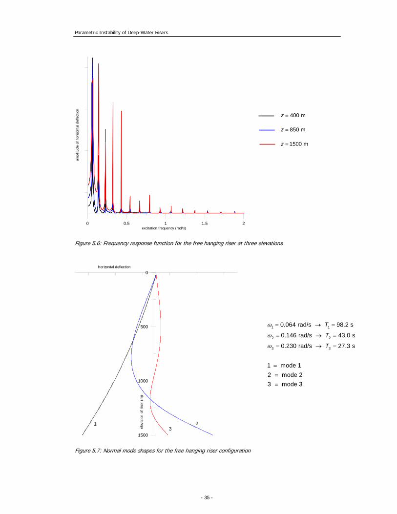
frequency for three elevations, viz. 400 m, 850 m, 1100 mz = . The excitation frequencies for which
the amplitudes reach a peak value correspond to the natural frequencies of the system. In Figure 5.3 the normal modes of the three lowest natural frequencies are plotted.
0 0.5 1 1.5 2excitation frequency (rad/s)
ampl
itude
of
horiz
onta
l def
lect
ion
Figure 5.2: Frequency response function for the simply supported riser at three elevations
400 mz =
850 mz =
1100 mz =

Parametric Instability of Deep-Water Risers
- 31 -
Figure 5.3: Normal mode shapes for the simply supported riser configuration The numerical results are exactly the same as the analytical results. This means that the program written in FORTRAN is correct.
5.3 Numerical approach: Model B and Model C 5.3.1 Introduction The equation of motion of the riser is given by equation [4.1]. In this analysis the time varying component of the tension is not included to enable calculation of the natural frequencies and normal modes. The differential equation is repeated below:
4 2
4 2
( , ) ( , ) ( , )( ) ( ) ( , )r f aw z t w z t w z tEI T z m m m f z t
z zz t∂ ∂ ∂ ∂⎡ ⎤− + + + =⎢ ⎥∂ ∂∂ ∂⎣ ⎦
[5.27]
in which:
topten( ) ( )( )s s wT z A g f L zρ ρ= − − [5.28]
iˆ( , ) tf z t fe ω= [5.29]
where: toptenf tensioning factor at riser top - fixed riser configuration =topten 1.3f
- free hanging riser configuration =topten 1.0f
1 10.155 rad/s 40.5 sTω = → =
2 20.311 rad/s 20.2 sTω = → =
3 30.466 rad/s 13.5 sTω = → =
1 mode 1= 2 mode 2= 3 mode 3=
horizontal deflection
1500
1000
500
0
elev
atio
n of
rise
r (m
)
3
2 1

Parametric Instability of Deep-Water Risers
- 32 -
f amplitude of the external force, arbitrarily chosen value [N/m] See Appendix A for the derivation of the effective tension term. Following the same procedure as in paragraph 5.2.3, the ordinary differential equation is given by:
4 2 2
4 2 2
ˆ ˆ ˆ ˆd d d d ˆˆ( )dd d d
w w w wEI z G w fzz z z
α β α ω+ − + + ⋅ = [5.30]
The coefficients used in equation [5.30] are given by:
( )s s wA gα ρ ρ= − [5.31]
topten( )s s wA g f Lβ ρ ρ= − [5.32]
2( ) ( ) ir f aG m m m cω ω ω= − + + ⋅ + ⋅ [5.33]
Equation [5.30] is an ordinary differential equation with a variable coefficient zα . This suggests that the analytical solution cannot be found straightforwardly because the solution cannot be expressed in terms of elementary functions due to this varying term. To integrate this differential equation the standard FORTRAN routine is used. With the definition of variables given by equation [5.24], equation [5.30] is written as the following system of first-order ordinary differential equations:
1 2
2 3
3 4
24 3 3 2 1 5
5 6
6 7
7 8
28 7 7 6 5 1
ˆ( ( ) ) /
( ( ) ) /
r f a
r f a
w w
w w
w w
w f z w w w m m m w c w EI
w w
w w
w w
w z w w w m m m w c w EI
α β α ω ω
α β α ω ω
⎡ ⎤ ⎡ ⎤′⎢ ⎥ ⎢ ⎥
′⎢ ⎥ ⎢ ⎥⎢ ⎥ ⎢ ⎥
′⎢ ⎥ ⎢ ⎥⎢ ⎥ ⎢ ⎥
′ − ⋅ + ⋅ − ⋅ + + + ⋅ + ⋅⎢ ⎥ ⎢ ⎥=⎢ ⎥ ⎢ ⎥′⎢ ⎥ ⎢ ⎥⎢ ⎥ ⎢ ⎥′⎢ ⎥ ⎢ ⎥⎢ ⎥ ⎢ ⎥′⎢ ⎥ ⎢ ⎥⎢ ⎥ ⎢ ⎥′ − ⋅ + ⋅ − ⋅ + + + ⋅ − ⋅⎣ ⎦ ⎣ ⎦
[5.34]
5.3.2 Results Model B – fixed riser The boundary conditions for the fixed riser are listed in paragraph 3.4.2. With the definition of variables given by equation [5.24], the boundary conditions become:

Parametric Instability of Deep-Water Risers
- 33 -
0 0.5 1 1.5 2excitation frequency (rad/s)
ampl
itude
of ho
rizon
tal d
e fle
ctio
n
1 2 1
2 3
5 5
6 7
ˆ(0) (0) ( ) 02
(0) ˆ ( ) 0
(0) 0 ( ) 0
(0) 0 ( ) 0
bw w u w L
w w L
w w L
w w L
ϕ
⎧ − = =⎪⎪⎪ = =⎪⎨⎪ = =⎪⎪⎪ = =⎩
[5.35]
In equation [5.35] u and ϕ represent the amplitudes of the two degrees of freedom of the
tension ring. These are defined by two equations of motion given by equation [3.15] and equation [3.16]. The equations below show these equations making use of the definition of variables given by [5.24]. Furthermore, the platform motions are assumed to be equal to zero.
2 20 0ring 4 0 2
vert vert
ˆ2 sin (0) (0) tan sin cos ˆ2
T Tk M u EI w T w k
L Lγ ω γ γ γ ϕ
⎛ ⎞ ⎛ ⎞+ − ⋅ = − ⋅ + ⋅ + ⋅ − ⋅ ⋅⎜ ⎟ ⎜ ⎟
⎝ ⎠ ⎝ ⎠
ll [5.36]
( )
2 22 2 20 0
0 ring 3vert
04 0 2
vert
tan tan cos ˆ (0)4 2 2 2
ˆ (0) (0) tan sin cos2 2
T T bk T J EI wL
Tb EI w T w k uL
γ γ γ ω ϕ
γ γ γ
⎛ ⎞⋅ + ⋅ + ⋅ − − ⋅ = ⋅⎜ ⎟
⎝ ⎠⎛ ⎞
+ − ⋅ + ⋅ + ⋅ − ⋅ ⋅⎜ ⎟⎝ ⎠
l ll
ll
[5.37]
The results of the FORTRAN program for the fixed riser are shown in Figure 5.4 and Figure 5.5. In Figure 5.4 the amplitudes of the horizontal displacement ˆ ( , )w z ω are plotted as function of the
excitation frequency for three elevations, viz. 400 m, 850 m, 1100 mz = . The excitation frequencies
for which the amplitudes reach a peak value correspond to the natural frequencies of the system. In Figure 5.5 the normal modes for the three lowest natural frequencies are plotted. Figure 5.4: Frequency response function for the fixed riser at three elevations
400 mz =
850 mz =
1100 mz =

Parametric Instability of Deep-Water Risers
- 34 -
Figure 5.5: Normal mode shapes for the fixed riser configuration Comment on figure From Figure 5.5 it can be concluded that the modes are not symmetric with respect to the mid-point of the riser. This is the result of the linear tension force along the riser.
5.3.3 Results Model C – free hanging riser The boundary conditions for the fixed riser are listed in paragraph 3.5.2. When the platform motions are assumed to be zero and with the definition of variables given by equation [5.24], the boundary conditions become:
1 3
2 4
5 7
6 8
(0) 0 ( ) 0
(0) 0 ( ) 0
(0) 0 ( ) 0
(0) 0 ( ) 0
w w L
w w L
w w L
w w L
⎧= =⎪
⎪⎪
= =⎪⎪⎨⎪ = =⎪⎪⎪ = =⎪⎩
[5.38]
The results for the free hanging riser configuration are shown in Figure 5.6 and Figure 5.7.
1 10.113 rad/s 55.6 sTω = → =
2 20.227 rad/s 27.7 sTω = → =
3 30.342 rad/s 18.4 sTω = → =
1 mode 1= 2 mode 2= 3 mode 3=
horizontal deflection
1500
1000
500
0
elev
atio
n of
rise
r (m
)
2
3 1
Parametric Instability of Deep-Water Risers
- 35 -
0 0.5 1 1.5 2excitation frequency (rad/s)
ampl
itude
of h
orizo
ntal
def
lect
ion
Figure 5.6: Frequency response function for the free hanging riser at three elevations
horizontal deflection
1500
1000
500
0
elev
atio
n of
rise
r (m
)
Figure 5.7: Normal mode shapes for the free hanging riser configuration
400 mz =
850 mz =
1500 mz =
1 10.064 rad/s 98.2 sTω = → =
2 20.146 rad/s 43.0 sTω = → =
3 30.230 rad/s 27.3 sTω = → =
1 mode 1= 2 mode 2= 3 mode 3=
1 3
2

Parametric Instability of Deep-Water Risers
- 36 -
5.4 Overview In this section a short overview of the results of the first part of this study is given, see Table 5.1. In the next part of this report, Part C, the time varying tension force is included in the equation of motion. This leads to a differential equation with a (periodic) time varying coefficient. This kind of excitation is called a parametric excitation. The natural frequencies and normal mode shapes as derived in this chapter are of great importance for determining the behaviour of the riser configurations under this parametric excitation.
Model A - simply supported riser, constant tension -
Model B - fixed riser -
Model C - free hanging riser -
Equation of Motion Equation of Motion Equation of Motion
4 2 2
4 2 2( ) ( , )r f aw w wEI T m m m f z t
z z t∂ ∂ ∂
− + + + =∂ ∂ ∂
4 2
4 2( ) ( ) ( , )r f aw w wEI T z m m m f z t
z z z t∂ ∂ ∂ ∂⎡ ⎤− + + + =⎢ ⎥∂ ∂ ∂ ∂⎣ ⎦
4 2
4 2( ) ( ) ( , )r f aw w wEI T z m m m f z t
z z z t∂ ∂ ∂ ∂⎡ ⎤− + + + =⎢ ⎥∂ ∂ ∂ ∂⎣ ⎦
Boundary Conditions Boundary Conditions Boundary Conditions
plat(0) ( )w u t= (0, ) ( ) ( )2bw t u t tϕ= + ⋅ plat(0, ) ( )w t u t=
2
2(0) 0w
z∂
=∂
(0, ) ( )w t tz
ϕ∂=
∂ plat
(0, ) ( )w t tz
ϕ∂=
∂
( , ) 0w L t = ( , ) 0w L t = 3
3
( , ) 0w L tz
∂=
∂
2
2
( , ) 0w L tz
∂=
∂
Schematic Representation
2
2
( , ) 0w L tz
∂=
∂
Schematic Representation
2
2
( , ) 0w L tz
∂=
∂
Schematic Representation
analytical solution AND numerical solver numerical solver - FORTRAN numerical solver - FORTRAN
First Natural Frequencies First Natural Frequencies First Natural Frequencies
1 0.155 rad/sω = 1 0.113 rad/sω = 1 0.064 rad/sω =
2 0.311 rad/sω = 2 0.227 rad/sω = 2 0.146 rad/sω =
3 0.466 rad/sω = 3 0.342 rad/sω = 3 0.230 rad/sω =
, EI m L
( , )f z t
platform
, EI m L
platform
( , )f z t
, EI m
kk
L
M
platform
( , )f z t

Parametric Instability of Deep-Water Risers
- 37 -

Parametric Instability of Deep-Water Risers
- 37 -
PART C
Riser Behaviour due to a Parametric Excitation
Semi-Submersible deep water drilling platform: Eirik Raude

Parametric Instability of Deep-Water Risers
- 38 -

Parametric Instability of Deep-Water Risers
- 39 -
6 Parametrically excited systems
6.1 Introduction In this chapter the time varying component of the tension force is included in the differential equation. This time dependent excitation appears as a coefficient in the governing equation of motion. This is called a parametric excitation. In section 6.2 a brief explanation of this phenomenon is given. This section is based on references [2-4]. Section 6.3 contains the derivation of the system of equations which is applicable to the three different riser configurations. In the final section the standard form of differential equations is given for a one-degree of freedom system and a two-degree of freedom system. These will be further analysed in Chapter 7. These differential equations are of the same form as in literature on the theory of dynamic stability [2-4].
6.2 Introduction to parametric excitation Among the problems of the dynamic stability of structures probably the best known subclass is constituted by the problems of parametric excitation, or parametric resonance. The equations of motion of this kind of problems are mathematically formulated as a system of differential equations with time-varying (periodic) coefficients. Two basic problems associated with these systems are of significant engineering importance: the dynamic stability of such systems and their response under various kinds of excitation. There are cases in which the introduction of a small vibrational loading can stabilize a system which is statically unstable or destabilize a system which is statically stable. Stephenson (1908) seems to have been the first to point out that a column under the influence of a periodic load may be stable even though the steady value of the load is twice that of the Euler load. Baliaev (1924) analyzed the response of a straight elastic hinged-hinged column to an axial periodic load. He showed that a column can be made to oscillate with one half of the excitation frequency of the periodic load if it is close to one of the natural frequencies of the lateral motion even though the load may be below the static buckling load of the column. Parametric resonance differs from resonance in the familiar sense of the term in two essential respects: - In ordinary resonance, the spectrum of frequencies at which vibrations with indefinitely
increasing amplitudes may build up is discrete: it is the set of natural frequencies of the system; in parametric resonance the spectrum is the union of several intervals. The widths of

Parametric Instability of Deep-Water Risers
- 40 -
the intervals depend on the amplitude of the perturbations and go to zero as the amplitude approaches zero.
- In ordinary resonance, the amplitudes of a dynamic system increase in accordance with a power law (generally linear), whereas in parametric resonance the increase is exponential; see Figure 2.2 (pp. 7).
Faraday (1831) seems to have been the first to observe the phenomenon of parametric resonance. He noted that surface waves in a fluid-filled cylinder under vertical excitation exhibited twice the period of the excitation itself. The problem of parametric resonance appears in many branches of physics and engineering. Some examples of real mechanical systems with time varying coefficients are listed below: - vibrations of suspension bridges - dynamic stability of a beam with an axial time varying load (e.g. marine risers) - helicopter rotor blades in forward flight - orbital stability of planar periodic motions of a satellite
6.3 Governing system of equations The system of equations will be derived for a periodic time varying component of the tension force. The shape of this component in z direction is not further specified. In the paragraphs 6.3.2 through 6.3.4 the three riser configurations will be treated separately. An overview of the governing system of equations is given in paragraph 6.3.5
6.3.1 General The time varying tension force is included in the equation of motion. The oscillating component is assumed to be simply harmonic. The resulting equation of motion yields:
( )4 2
4 2
( , ) ( , ) ( , )( ) ( )cos ( ) 0r f aw z t w z t w z tEI T z S z t m m m
z zz t∂ ∂ ∂ ∂⎡ ⎤− + Ω + + + =⎢ ⎥∂ ∂∂ ∂⎣ ⎦
[6.1]
where:
( )T z static component of the tension force [N]
( )S z amplitude of time varying component of the tension force [N]
Ω frequency of parametric excitation [rad/s] The partial differential equation [6.1] is reduced to a system of ordinary differential equations by using the Galerkin’s Method. When using this method, one represents the solution ( , )w z t in
terms of an orthogonal function expansion where each trial function satisfies the boundary conditions. In this case the normal mode shapes ( )n zφ of the system without the time-dependent
tension are used as trial functions. A solution to equation [6.1] is written in the form:
1( , ) ( ) ( )n n
nw z t z q tφ
∞
=
= ⋅∑ [6.2]

Parametric Instability of Deep-Water Risers
- 41 -
where: ( )n zφ displacement amplitude of nth normal mode [m]
( )nq t unknown function of time [-]
The expressions for ( )n zφ are determined in Part B for three riser configurations. These normal
modes are the eigenfunctions of the problem:
42
4
d ( ) d d ( )( ) ( ) ( ) 0d dd r f a n
z zEI T z m m m zz zz
φ φ ω φ− − + + ⋅ ⋅ = [6.3]
where nω is the natural frequency of nth normal mode [rad/s]
A property of eigenfunctions is that these are orthogonal:
0
0L
m ndzφ φ⋅ =∫ if m n≠ [6.4]
Substituting equation [6.2] into equation [6.1] yields:
( )( ) ( ) ( ) ( ) ( )cos ( ) ( ) ( ) ( ) ( ) 0n n n n r f a n nn
EI z q t T z S z t z q t m m m q t zz
φ φ φ∂⎡ ⎤′′′′ ′− + Ω + + + ⋅ =⎢ ⎥∂⎣ ⎦∑ && [6.5]
Using equation [6.3], equation [6.5] can be rewritten in the following form:
( )( ) ( )2( ) ( ) ( ) ( )cos ( ) ( ) 0r f a n n n n n nn
m m m q t q t z S z t z q tz
ω φ φ∂⎡ ⎤′+ + + − Ω ⋅ =⎢ ⎥∂⎣ ⎦∑ && [6.6]
After rewriting equation [6.6], equation [6.7] is obtained:
( ) ( ) ( )2 cos( ) ( ) ( ) ( ) ( ) ( ) ( ) ( ) 0n n n n n n nn r f a
tq t q t z S z z S z z q tm m m
ω φ φ φ⎡ ⎤Ω ′′ ′ ′+ − ⋅ + ⋅ =⎢ ⎥
+ +⎢ ⎥⎣ ⎦∑ && [6.7]
Multiplying equation [6.7] by mφ , integrating the result from 0z = to z L= and using the
orthogonality condition [6.4], the following expression is obtained:
( ) ( )2 2
0 0
cos ( ) ( ) ( ) ( ) 0( )
L L
m m m m n n m nnr f a
tq q dz S z z S z z dz qm m m
ω φ φ φ φ⎡ ⎤Ω ′′ ′ ′+ ⋅ − ⋅ + ⋅ =⎢ ⎥+ + ⎣ ⎦
∑∫ ∫&& ,
1, 2, 3....,m n= [6.8]
In a mathematically simplified form, equation [6.8] yields:
( )2 cos 0( ) m m m mn mn n
nr f a
tq q f g qm m m
ω Ω+ − + =
+ + ∑&& , 1, 2, 3....,m n= [6.9]

Parametric Instability of Deep-Water Risers
- 42 -
where:
0
2
0
( )L
m n
mn L
m
S z dzf
dz
φ φ
φ
′′⋅ ⋅=∫
∫ [6.10]
0
2
0
( )L
m n
mn L
m
S z dzg
dz
φ φ
φ
′′ ⋅ ⋅=∫
∫ [6.11]
6.3.2 System of equations for simply supported riser - Model A This paragraph contains the set of linear equations for Model A, the simply supported riser with constant tension. For this simplified case the amplitude of the time varying component of the tension force is constant along the riser:
( )S z S= [6.12]
The set of equations [6.9] yields:
2 cos 0( ) m m m mn n
nr f a
S tq q f qm m m
ω Ω+ − =
+ + ∑ %&& , 1, 2, 3....,m n= [6.13]
where:
0
2
0
L
m n
mn L
m
dzf
dz
φ φ
φ
′′⋅=∫
∫% [6.14]
The normal modes for this particular case are defined by:
sinnn z
Lπφ ⎛ ⎞= ⎜ ⎟
⎝ ⎠ [6.15]
This expression for the normal modes implies:
if m n≠ : 0
0 L
m n dzφ φ ′′⋅ =∫ 0mnf =%
Thus, the system becomes decoupled and the differential equation for the n th natural frequency is given by:

Parametric Instability of Deep-Water Risers
- 43 -
2 0
2
0
cos 0( )
L
n n
n n n nLr f a
n
dzS tq q q
m m mdz
φ φω
φ
′′⋅Ω
+ − ⋅ =+ +
∫
∫&& [6.16]
6.3.3 System of equations for fixed riser - Model B This paragraph contains the set of coupled linear equations for Model B, the fixed riser configuration. See Appendix A for the derivation of the time varying component of tension force,
( , )S z t . In line with the results of this appendix the amplitude of the time varying component of
the tension force is constant along the riser. So the equations [6.17] through [6.19] are the same as the equations [6.12] through [6.14].
( )S z S= [6.17]
The set of equations yields:
2 cos 0( ) m m m mn n
nr f a
S tq q f qm m m
ω Ω+ − =
+ + ∑ %&& , 1, 2, 3....,m n= [6.18]
where:
0
2
0
L
m n
mn L
m
dzf
dz
φ φ
φ
′′⋅=∫
∫% [6.19]
6.3.4 System of equations for free hanging riser - Model C This paragraph contains the set of coupled linear equations for Model C, the free hanging riser configuration. In line with the results of Appendix A the amplitude of the time varying component of the tension force is linear along the riser:
max( ) 1 zS z SL
⎛ ⎞= −⎜ ⎟⎝ ⎠
[6.20]
in which maxS is the amplitude of the time varying tension at the riser top.
In this case the set of equations yields:
( )2 max cos0
( ) m m m mn mn nnr f a
S tq q f g q
m m mω
⋅ Ω+ − + =
+ + ∑ %&& % , 1, 2, 3....,m n= [6.21]

Parametric Instability of Deep-Water Risers
- 44 -
where:
( )0
2
0
1L
m n
mn L
m
z L dzf
dz
φ φ
φ
′′− ⋅ ⋅=∫
∫% [6.22]
0
2
0
L
m n
mn L
m
dzg
L dz
φ φ
φ
′⋅= −
⋅
∫
∫% [6.23]
Comment The coupling factors given by equations [6.22] and [6.23] can be replaced by one coupling term. To obtain this term equation [6.8] is rewritten in the following form:
( ) ( )2 2
0 0
cos ( ) 0( )
L L
m m m m n m nnr f a
t dq q dz S z dz qm m m dz
ω φ φ φ⎡ ⎤Ω ′+ ⋅ − ⋅ =⎢ ⎥+ + ⎣ ⎦
∑∫ ∫&& , 1, 2, 3....,m n= [6.24]
In a mathematically simplified form:
( )2 cos 0( ) m m m mn n
nr f a
tq q f qm m m
ω Ω+ − =
+ + ∑ %&& , 1, 2, 3....,m n= [6.25]
where:
( )0
2
0
( )L
n m
mn L
m
d S z dzdz
fdz
φ φ
φ
′ ⋅=∫
∫% [6.26]
The expression ( )0
( )L
n md S z dzdz
φ φ′ ⋅∫ can be rewritten by using the technique of integration by
parts. The definition of integration by parts yields:
udv uv vdu= −∫ ∫ [6.27]
For this case:
( )( ) nddv S z dzdz
φ′= and mu φ=
This leads to the following expression:

Parametric Instability of Deep-Water Risers
- 45 -
( ) 00 0 0
( ) ( ) ( ) ( ) ( ) ( ) (0) (0) (0) ( )L L L
Ln m m n m n m n m n m n
d S z dz S z S z dz S L L L S S z dzdz
φ φ φ φ φ φ φ φ φ φ φ φ′ ′ ′ ′ ′ ′ ′ ′⋅ = − = − −∫ ∫ ∫
in which ( ) 0S L = and (0) 0mφ = . This second condition holds because this is one of the
boundary conditions. So equations [6.25] and [6.26] can be written as:
( )2 max cos0
( ) m m m mn nnr f a
S tq q f q
m m mω
⋅ Ω+ − =
+ + ∑ %%&& , 1, 2, 3....,m n= [6.28]
( )0
2
0
1L
m n
mn L
m
z L dzf
dz
φ φ
φ
′ ′− ⋅ ⋅= −∫
∫
%% [6.29]
6.3.5 Overview of the system of equations In this section a short overview of the results of this section is given, see Table 6.1. In Chapter 8 these sets of differential equations will be further analysed to obtain the combinations of magnitude and frequency of the time varying force which leads to parametric resonance for the three riser configurations.
Model A -simply supported riser, constant tension-
Model B -fixed riser-
Model C -free hanging riser-
Equation of Motion Equation of Motion Equation of Motion
4 2 2
4 2 2( ) ( ) 0r f aw w wEI T t m m m
z z t∂ ∂ ∂
− + + + =∂ ∂ ∂
4 2
4 2( , ) ( ) 0r f aw w wEI T z t m m m
z z z t∂ ∂ ∂ ∂⎡ ⎤− + + + =⎢ ⎥∂ ∂ ∂ ∂⎣ ⎦
4 2
4 2( , ) ( ) 0r f aw w wEI T z t m m mz z z t
∂ ∂ ∂ ∂⎡ ⎤− + + + =⎢ ⎥∂ ∂ ∂ ∂⎣ ⎦
Tension force Tension force Tension force
( ) cos( )T t T S t= + Ω ( , ) ( ) cos( )T z t T z S t= + Ω ( )max( , ) ( ) 1 cos( )T z t T z S z L t= + ⋅ − Ω
Set of equations - decoupled Set of equations – coupled Set of equations - coupled
2 cos 0( )n n n nn n
r f a
S tq q f qm m m
ω Ω+ − ⋅ =
+ +%&& 2 cos 0
( ) m m m mn nnr f a
S tq q f qm m m
ω Ω+ − =
+ + ∑ %&& 2 max cos 0( ) m m m mn n
nr f a
S tq q f qm m m
ω ⋅ Ω+ − =
+ + ∑ %%&&
0
2
0
L
n n
nn L
n
dzf
dz
φ φ
φ
′′⋅=∫
∫% , 0mnf =% if m n≠ 0
2
0
L
m n
mn L
m
dzf
dz
φ φ
φ
′′⋅=∫
∫%
( )0
2
0
1L
m n
mn L
m
z L dzf
dz
φ φ
φ
′ ′− ⋅ ⋅= −∫
∫
%%
Table 6.1: Overview of the set of equations for three riser configurations

Parametric Instability of Deep-Water Risers
- 46 -
6.4 Standard form of differential equations containing variable coefficients
A vast amount of classical literature exists on the subject of stability of ordinary differential equations with periodic coefficients; see references [2-6]. In this section the systems of differential equations of the previous section are written in a more common form as used in this literature. System of uncoupled differential equations – Model A The simplest differential equation with periodic coefficients is the Mathieu equation
( cos2 ) 0q t qδ ε+ + =&& [6.30]
where δ and ε are constants. This equation governs the response of many physical systems (having one degree of freedom) to a sinusoidal parametric excitation. An example is a pendulum consisting of a uniform rod pinned at a point on a platform that is made to oscillate sinusoidally in vertical direction. This system has one degree of freedom: the angular rotation of the rod. The simply supported riser with constant tension, Model A, is a multi-degree of freedom system. Nevertheless, it can be analysed in the same manner as a one-degree of freedom system because the modes are uncoupled. So the Mathieu equation is valid for every mode. In literature the equations corresponding to the analysed systems are often written in the same form as the Mathieu equation. However, in Chapter 7 it is chosen not to analyse the Mathieu equation, but equation [6.31], given by:
( )20( ) 1 cos ( ) 0q t t q tω ε+ + Ω =&& % [6.31]
In this equation 0ω stands for the natural frequency of the analysed mode. The advantage of
this notation is that the parameter ε% is dimensionless. Its value shows directly if it is possible to
apply a small parameter method. This is allowed if the following condition is satisfied: 1ε% .
Comparing equation [6.31] with the set of equations as shown in Table 6.1, equation [6.31] is exactly of the same form as the equation for the simply supported riser with constant tension where:
0 nω ω= [6.32]
02
2
0
( )
L
n n
Ln r f a
n
dzS
m m mdz
φ φε
ωφ
′′⋅= − ⋅
⋅ + +
∫
∫% [6.33]
System of coupled differential equations – Model B and Model C Literature on multi-degree of freedom systems that are parametrically excited by one excitation considers the system given by equation [6.34]:

Parametric Instability of Deep-Water Risers
- 47 -
2
1cos 0
N
n n n nm mm
q q t f qω ε=
+ + Ω =∑&& , where 1, 2,....n N= [6.34]
In this equation N may be any positive integer and ε is a small dimensionless parameter. Comparing equation [6.34] with the sets of equations as shown in Table 6.1, equation [6.34] is exactly of the same form as the equations for the fixed and free hanging riser. In Chapter 7 several methods are applied to the set of equations given by [6.34] to obtain the combinations of Ω and ε for which the solution ( )q t is unstable. For simplicity the number of
degrees of freedom is chosen equal to two:
( )
( )
21 1 1 11 1 12 2
22 2 2 21 1 22 2
( ) ( ) cos ( ) ( ) 0
( ) ( ) cos ( ) ( ) 0
q t q t t f q t f q t
q t q t t f q t f q t
ω ε
ω ε
⎧ + + Ω + =⎪⎨⎪ + + Ω + =⎩
&&
&&
[6.35]

Parametric Instability of Deep-Water Risers
- 48 -

Parametric Instability of Deep-Water Risers
- 49 -
7 Methods to analyse the dynamic stability
7.1 Introduction In this chapter three methods to analyse dynamic stability of systems are presented: - Small parameter method, also known as Perturbation method; section 7.2 - Floquet theory; section 7.3 - Hill’s method of infinite determinants; section 7.4 In each section a brief review of these methods is given. This review is followed by the application of the method to the differential equation for a one-degree of freedom system and the set of equations for a two-degree of freedom system. These equations are repeated below: One-degree of freedom system
( )20( ) 1 cos ( ) 0q t t q tω ε+ + Ω =&& % [7.1]
Two-degree of freedom system
( )
( )
21 1 1 11 1 12 2
22 2 2 21 1 22 2
( ) ( ) cos ( ) ( ) 0
( ) ( ) cos ( ) ( ) 0
q t q t t f q t f q t
q t q t t f q t f q t
ω ε
ω ε
⎧ + + Ω + =⎪⎨⎪ + + Ω + =⎩
&&
&&
[7.2]
In section 7.5 an overview of the characteristics of all three methods is given. The most suitable method, the Floquet Theory, will be used in Chapter 8 to obtain the stability charts for the systems of equations corresponding to the riser cases as described in Chapter 6.
7.2 Small parameter method
7.2.1 General A small parameter method is only suited for determination of the stability if the time varying component of the tension force is relatively small, i.e. the parameter ε% in equation [7.1] is a small parameter:

Parametric Instability of Deep-Water Risers
- 50 -
1ε% [7.3a]
and the parameter ( ) 2
mn nfε ω in the system of equations given by equation [7.2] is a small
parameter:
( ) 2 1mn nfε ω [7.3b]
In this paragraph we presume that the conditions given in [7.3] are satisfied. Accordingly we seek for a solution in the form of an expansion:
2 3,0 ,1 ,2( ; ) ( ) ( ) ( ) ( )n n n nq t q t q t q t Oε ε ε ε= + + + [7.4]
where n refers to the number of degrees of freedom. This straightforward expansion is an analytical approximation method. The series expansion ( ; )nq t ε is a valid solution as long as the
terms in this solution do not grow faster in time than the terms corresponding to a lower power of ε . For certain parametric excitation frequencies this requirement is not fulfilled. As a consequence the total solution explodes and will not converge. The excitation frequencies that cause this effect in the approximation are to be found, because these frequencies equal the main frequencies of parametric resonance and allocate the instability zones. In paragraph 7.2.2 the expansion given by equation [7.4] is substituted into equation [7.1] and in paragraph 7.2.3 this expansion is substituted into equation [7.2].
7.2.2 One-degree of freedom system The different possible resonant conditions can be exhibited by a straightforward expansion given by equation [7.4]. The index n is skipped from the equation because the analysed system is a one-degree of freedom system. Substituting equation [7.4] into equation [7.1] and equating coefficients of like powers of ε% yields:
20 0 0( ) ( ) 0q t q tω+ =&& [7.5]
2 2
1 0 1 0 0( ) ( ) cos ( )q t q t t q tω ω+ = − Ω ⋅&& [7.6]
2 2
2 0 2 0 1( ) ( ) cos ( )q t q t t q tω ω+ = − Ω ⋅&& [7.7]
The general solution of equation [7.5] can be written in the form:
0 0 0 0 0( ) sin cosq t A t B tω ω= + [7.8]
Substituting equation [7.8] into equation [7.6] yields:
( )2 21 0 1 0 0 0 0 0( ) ( ) cos sin cosq t q t t A t B tω ω ω ω+ = − Ω ⋅ +&& [7.9]

Parametric Instability of Deep-Water Risers
- 51 -
The particular solution of this equation will contain small divisors for the following excitation frequencies:
0 02 , 2 , 0ω ωΩ = + Ω = − Ω = [7.10]
The excitation frequencies as defined in equation [7.10] will lead to unbounded solutions for the first order term 1( )q t . Appendix E-1 contains the MAPLE output which shows the complete
derivation of these results. Repeating the same procedure for the second-order term of ( )q t , the expansion [7.4] is not valid
for the following excitation frequencies:
0 0, , 0ω ωΩ = + Ω = − Ω = [7.11]
The general result is that for a small value of ε% unstable oscillations exist for the system defined by equation [7.1] under the following condition:
02pω
Ω = ± [7.12]
where: p integer, defining the order of the instability zone [-]
This result shows that the proposed solution technique, expansion [7.4], is not valid in the neighbourhood of the excitation frequencies defined by equation [7.12]. To obtain the boundaries between stable and unstable solutions in the first instability zone ( 02ωΩ = ) the
solution of 0 ( )q t given by equation [7.8] is enhanced. This should be done in such a manner that
the troublesome terms of 1( )q t that lead to unbounded solutions are eliminated. Therefore, the
general solution of 0 ( )q t is modified in the following general expression:
( ) ( )0 0 0( ) ( )sin ( ) ( )cos ( )q t A t t B t tε ω εσ ε ω εσ= + + +% % % % [7.13]
This enhances the series expansion to the following form:
( ) ( ) 20 0 1 2( ) ( )sin ( ) ( )cos ( ) ( ) ( )q t A t t B t t q t q tε ω εσ ε ω εσ ε ε= + + + + +% % % % % % [7.14]
Substituting equation [7.14] into equation [7.1] and equating coefficients of power 1ε% yields:
( ) ( )
( ) ( ) ( )
( )
21 0 1 0 0 0 0
210 0 0 0 0 02
2 21 10 0 02 2
( ) ( ) 2 ( ) sin ( ) 2 ( ) cos ( )
2 ( ) cos ( ) 2 ( ) sin ( ) ( )cos ( )
( )sin ( ) (
q t q t A t t A t t
B t t B t t B t t
A t t A
ω ε ω σ ω εσ ε ω ω εσ
ε ω σ ω εσ ε ω ω εσ ω ε ω εσ
ω ε ω εσ ω
+ = + − +
+ + + + − −Ω + +
− −Ω + + −
&&& % % % %
&% % % % % %
% % ( ) ( )210 0 02)sin ( ) ( )cos ( )t t B t tε ω εσ ω ε ω εσΩ + + − Ω + +% % % %
[7.15]

Parametric Instability of Deep-Water Risers
- 52 -
In the region around the first main frequency of parametric resonance, 02ωΩ = , the first six
terms in equation [7.15] will lead to an unbounded solution. If these terms have the same argument, it is possible to set the amplitudes of these sine terms and cosine terms equal to zero. As a result of this demand, the expression for the excitation frequency is given by:
02 2ω εσΩ = + % [7.16]
Substituting this expression into equation [7.15] yields:
( )
( )
2 211 0 1 0 0 0 02
210 0 0 02
2102
( ) ( ) 2 ( ) 2 ( ) ( ) sin ( )
2 ( ) 2 ( ) ( ) cos ( )
(
q t q t A t B t A t t
A t B t B t t
A t
ω ε ω σ ε ω ω ε ω εσ
ε ω ε ω σ ω ε ω εσ
ω ε
⎡ ⎤+ = + + +⎣ ⎦
⎡ ⎤+ − + − +⎣ ⎦
−
&&& % % % %
& % % % %
% ( ) ( )210 0 02)sin (3 3 ) ( )cos (3 3 )t B t tω εσ ω ε ω εσ+ − +% % %
[7.17]
In order to eliminate all resonance terms in equation [7.17] the following system of first order differential equations for the coefficients ( )A tε and ( )B tε is obtained:
( )
( )
210 0 02
210 0 02
( )2 2 ( ) 0
( )2 2 ( ) 0
dB t A tdt
dA t B tdt
εω ω σ ω ε
εω ω σ ω ε
⎧ + + =⎪⎪⎨⎪⎪− + − =⎩
%%
%%
[7.18]
The general solution of this system of first order differential equations is given by:
0
0
( ) exp( )
( ) exp( )
A t A t
B t B t
ε λε
ε λε
=⎧⎪⎨⎪ =⎩
% %
% %
[7.19]
Substituting the general solution into the system of equations given by [7.18] leads to a system of two algebraic equations; an eigenvalue problem. Such a system has a non-trivial solution if its determinant is equal to zero. This yields the characteristic equation:
2 2 4 2 2 210 0 044 4 0ω σ ω λ ε ω− + =% [7.20]
A stable motion of ( )q t requires: Re( ) 0λ ≤ . Setting 0λ = and substituting expression [7.16]
into equation [7.20] leads to the following boundary between stable and unstable motions:
10 022ω ω εΩ = + % [7.21a]
1
0 022ω ω εΩ = − % [7.21b]
The same procedure can be repeated to obtain an accurate solution of the order 2ε% . The solution
2( )q t contains also troublesome terms which should be eliminated.

Parametric Instability of Deep-Water Risers
- 53 -
0 5 10 15 20 25Excitation period (s)
0
0.2
0.4
0.6
0.8
1
epsi
lon
(-)
Landau [7] shows that the transition curves of an accuracy of the order 2ε% are given by:
21 10 0 02 322ω ω ε ω εΩ = + −% % [7.22a]
21 10 0 02 322ω ω ε ω εΩ = − −% % [7.22b]
For the instability zone of the second order the following expressions hold:
210 048ω ω εΩ = − % [7.23a]
250 048ω ω εΩ = + % [7.23b]
and for the third order:
22 10 03 64ω ω εΩ = − % [7.24a]
22 10 03 64ω ω εΩ = + % [7.24b]
In Figure 7.1 these instability zones are shown for 0 0.5ω = rad/s.
Figure 7.1: Stability chart containing first three instability zones (p=1 through 3)
Comment on figure The dashed red lines show the transition curves that satisfies equation [7.22] through equation [7.24]. However, the corresponding values of ε% do not satisfy equation [7.3a]. This implies that this method is in
fact not applicable for these values of ε% .
7.2.3 Two-degree of freedom system The different possible resonant conditions for a two-degree of freedom system can be exhibited by a straightforward expansion given by equation [7.4]. Substituting equation [7.4] into equation [7.2] and equating coefficients of like powers of ε yields:
1ε <<% , small parameter
0ω 02ω 203ω

Parametric Instability of Deep-Water Risers
- 54 -
21,0 1 1,0
22,0 2 2,0
( ) ( ) 0
( ) ( ) 0
q t q t
q t q t
ω
ω
⎧ + =⎪⎨⎪ + =⎩
&&
&&
[7.25]
( )
( )
21,1 1 1,1 11 1,0 12 2,0
22,1 2 2,1 21 1,0 22 2,0
( ) ( ) cos ( ) ( )
( ) ( ) cos ( ) ( )
q t q t t f q t f q t
q t q t t f q t f q t
ω
ω
⎧ + = − Ω ⋅ +⎪⎪⎨⎪ + = − Ω ⋅ +⎪⎩
&&
&&
[7.26]
( )
( )
21,2 1 1,2 11 1,1 12 2,1
22,2 2 2,2 21 1,1 22 2,1
( ) ( ) cos ( ) ( )
( ) ( ) cos ( ) ( )
q t q t t f q t f q t
q t q t t f q t f q t
ω
ω
⎧ + = − Ω ⋅ +⎪⎪⎨⎪ + = − Ω ⋅ +⎪⎩
&&
&&
[7.27]
The general solution of equation [7.25] can be written in the form:
1,0 1,0 1 1,0 1
2,0 2,0 2 2,0 2
( ) sin cos
( ) sin cos
q t A t B t
q t A t B t
ω ω
ω ω
= +⎧⎪⎨⎪ = +⎩
[7.28]
Substituting the set of equations [7.28] into equation [7.26] yields:
( ) ( )( )
( ) ( )( )
21,1 1 1,1 11 1,0 1 1,0 1 12 2,0 2 2,0 2
22,1 2 2,1 21 1,0 1 1,0 1 22 2,0 2 2,0 2
( ) ( ) cos sin cos sin cos
( ) ( ) cos sin cos sin cos
q t q t t f A t B t f A t B t
q t q t t f A t B t f A t B t
ω ω ω ω ω
ω ω ω ω ω
⎧ + = − Ω ⋅ + + +⎪⎪⎨⎪ + = − Ω ⋅ + + +⎪⎩
&&
&&
[7.29]
The particular solutions of these two equations will contain small divisors for the following excitation frequencies:
1 2 1 22 , 2 ,ω ω ω ωΩ = ± Ω = ± Ω = ± ± [7.30]
The excitation frequencies as defined in equation [7.30] will lead to unbounded solutions for the first order terms 1,1( )q t and/or 2,1( )q t . Appendix E-2 contains the MAPLE output which shows the
complete derivation of these results. Repeating the same procedure for the second-order term of 1( )q t and 2( )q t , the expansion [7.4]
is not valid for the following excitation frequencies:
1 11 2 1 22 2, ,ω ω ω ωΩ = ± Ω = ± Ω = ± ± [7.31]
The general result is that for a small value of ε unstable oscillations exist for the system defined by equation [7.2] under the following condition:
m np ω ω⋅Ω = ± , 0Ω ≠ [7.32]

Parametric Instability of Deep-Water Risers
- 55 -
where: p integer, the absolute value of p defines the order of the instability zone [-]
One speaks of simple resonance when m n= . Combination resonance occurs when m n≠ . This result shows that the proposed solution technique, expansion [7.4], is not valid in the neighbourhood of the excitation frequencies defined by equation [7.32]. To obtain the boundaries between stable and unstable solutions in these zones the same method as for the one-degree of freedom is applied. In reference [3] this method is extensively investigated for the instability zones of the first order. Here the results of this research are listed. The instability zones of the first order, i.e. the principal regions of instability, are given by the following expressions: Combination resonance
- ( )
212
1 21 2
2 2 2 2 2 2 212 1 22 2 212 22 11 21 22 111
1 28 2 2 2 2 2 21 2 2 1 2 1 1 2 2 1 2 1 2 1
2
1 1 2 2
4 ( 2 ) (2 ) ( ) ( )
f
f f f f f f f
ω ω εω ω
ω ωε ω ω
ω ω ω ω ω ω ω ω ω ω ω ω ω ω
Ω = + ±
⎡ ⎤+ + +− − − + + − −⎢ ⎥
+ + − −⎢ ⎥⎣ ⎦ [7.33]
- ( )
212
1 21 2
2 2 2 2 2 2 212 1 22 2 212 22 11 21 22 111
1 28 2 2 2 2 2 21 2 2 1 2 1 1 2 2 1 2 1 2 1
2
1 1 2 2
4 ( 2 ) (2 ) ( ) ( )
f
f f f f f f f
ω ω εω ω
ω ωε ω ω
ω ω ω ω ω ω ω ω ω ω ω ω ω ω
Ω = − + ±
⎡ ⎤+ + +− − − + + − −⎢ ⎥
+ + − −⎢ ⎥⎣ ⎦ [7.34]
Simple resonance
- 2 2 2
211 11 12 121 3 2 2 2 2
1 1 1 1 2 1 1 2
f 2
2 8 (9 ) ( )f f f
ω ε εω ω ω ω ω ω ω ω
⎡ ⎤Ω = ± − − −⎢ ⎥− −⎣ ⎦
[7.35]
- 2 2 2
222 22 21 212 3 2 2 2 2
2 2 2 2 1 2 2 1
f2
2 8 (9 ) ( )f f f
ω ε εω ω ω ω ω ω ω ω
⎡ ⎤Ω = ± − − −⎢ ⎥− −⎣ ⎦
[7.36]
In Figure 7.2 three instability zones of the first order are shown for the following case:
1 0.2ω = rad/s and 2 0.5ω = rad/s
11 12 21 22 1.0f f f f= = = = s-2

Parametric Instability of Deep-Water Risers
- 56 -
0 5 10 15 20 25Excitation period (s)
0
0.03
0.06
0.09
0.12
0.15
epsi
lon
(-)
Figure 7.2: Stability chart containing instability zones of first order (p=1) Comment on figure The dashed red lines show the transition curves that satisfies equation [7.33] through equation [7.36]. However, the corresponding values of ε do not satisfy equation [7.3b]. This implies that this method is in
fact not applicable for these ‘large’ values of ε .
7.3 Floquet theory
7.3.1 General A straightforward method for dealing with the stability of a system of ordinary differential equations with periodic coefficients contains in applying the Floquet theory. This theory provides a quantitative measure of the stability of a system consisting of first-order differential equations. Both equations [7.1] and [7.2] can be rewritten as a system of first-order differential equations. These systems can be written in the following general form:
( ) ( ) ( )x t A t x t= ⋅& [7.37]
The matrix ( )A t is an ( )nxn -matrix.
A new quantity will be introduced which is necessary to analyse this system: the state transition matrix or fundamental matrix 0( , )t tΦ . The definition of this matrix is:
1
0 0( , ) ( ) ( )t t U t U t−Φ = ⋅ [7.38]
where ( )U t is the fundamental solution matrix. This matrix contains n linearly independent
solutions to equation [7.37]. This matrix has the following form:
( ) ( ) ( )1 2( ) , ,....,t t t
nU t x x x⎡ ⎤= ⎣ ⎦ [7.39]
( ) 2 1mn nfε ω << , small parameter
12ω 22ω
1 2ω ω+
1 2ω ω− +

Parametric Instability of Deep-Water Risers
- 57 -
where ( )tix is a vector containing the i th independent solution to equation [7.37].
The state transition matrix at time 0t = is defined by the identity matrix:
(0,0) nΦ = Ι [7.40]
The Floquet Theorem states:
If ( ) ( )A t A t T= + , then ( ,0) ( ,0) tFt L t eΦ = ⋅ , [7.41]
Where ( ,0) ( ,0)L t L t T= +
F is a constant
The matrix exponential in equation [7.41] is defined by the following power series:
0 !
ntF
n
tFe
n
∞
=
= ∑
From this theorem and the equations stated above it follows that:
(0,0) ( ,0) nL L T= = Ι [7.42]
1 ln ( ,0)F TT
= Φ [7.43]
The Lyapunov Reducibility Theorem states:
( ) ( ,0) ( )x t L t z t= ⋅ change of variables
This change of variables transforms the system given by equation [7.37] into a linear time invariant system:
( ) ( )z t F z t= ⋅& [7.44]
For the case of a linear system with constant coefficients ( ) ( )z t F z t= ⋅& , the eigenvalues of F
determine the stability of the solution. If one of these eigenvalues has a real positive part, the solution ( )z t will grow exponentially in time:
( )0( ) exp ( ) (0)z t F t t z= ⋅ − ⋅ [7.45]
From equation [7.43] it can be concluded that the stability criterion for the system is related to the eigenvalues of the state transition matrix at the end of one period. Consequently, the solutions of equations [7.37] approach zero as t → ∞ if: Stability criterion: 2 2(Re ) (Im ) 1i iλ λ+ < 1, 2...,i n= [7.46]
⎫⎬⎭
complex values

Parametric Instability of Deep-Water Risers
- 58 -
where iλ are the eigenvalues of the state transition matrix at the end of one period.
By definition of the fundamental matrix solution given in equation [7.39] the following relation holds:
( )U A t U= ⋅& [7.47]
Thus, the state transition matrix at an arbitrarily chosen moment in time is given by:
( ,0) ( ) ( ,0)t A t tΦ = ⋅Φ& , 0 0t = [7.48]
The transition matrix at the end of one period, ( ,0)TΦ , can be computed numerically by
integrating the matrix differential equation [7.48] over one period 2T π= Ω with the initial
condition (0,0) nΦ = Ι . If one of the eigenvalues of ( ,0)TΦ is larger than 1.0 we can conclude
that the system is unstable.
7.2.2 One-degree of freedom system To use the Floquet theory equation [7.1] should be rewritten to a system of first-order differential equations by defining
1( ) ( )x t q t= [7.49]
2( ) ( )x t q t= & [7.50]
so that equation [7.1] becomes:
1 1202 2
0 1( ) ( )(1 cos ) 0( ) ( )
x t x ttx t x tω ε
⎡ ⎤⎡ ⎤ ⎡ ⎤= ⋅⎢ ⎥⎢ ⎥ ⎢ ⎥− + Ω⎣ ⎦ ⎣ ⎦⎣ ⎦
&
& % [7.51]
Anticipating on the riser case a damping term will be included in the system. It is very easy to include a damping term c which is proportional to 2( )x t . This implies for the riser configuration
a damping term which is proportional to the velocity of the riser. The time dependent matrix ( )A t of equation [7.48] becomes:
20
0 1( )
(1 cos )A t
t cω ε⎡ ⎤
= ⎢ ⎥− + Ω −⎣ ⎦% [7.52]
The system which has to be analyzed for all possible combinations of ε% and Ω is defined by ( ,0) ( ) ( ,0)t A t tΦ = ⋅Φ& [7.53]
where the time-dependent matrix ( )A t is given by equation [7.52] and the initial condition
(0,0)Φ is equal to 2Ι .

Parametric Instability of Deep-Water Risers
- 59 -
0 5 10 15 20 25Excitation Period (s)
0
1
2
3
4
5
epsi
lon
(-)
0 5 10 15 20 25Excitation Period (s)
0
1
2
3
4
5
epsi
lon
(-)
A program is written in FORTRAN to compute numerically ( ,0)TΦ and the corresponding
eigenvalues of this matrix. The used routine in FORTRAN to obtain ( ,0)TΦ applies the Runge-
Kutta method to solve the initial value problem defined by equation [7.53]. The results are shown in a stability chart in Figure 7.3 and Figure 7.4. The combinations of ε% and Ω that lead to instability are indicated by a dot. These dots together form several instability zones. Figure 7.3 is for the case of no damping and Figure 7.4 for the case of 0.1c = s-1. The stability charts are obtained for a system in which 0 0.5ω = rad/s.
Figure 7.3: Stability chart, no damping Figure 7.4: Stability chart, including damping Comment on figures
Figure 7.4 shows that in case of damping the value of ε% should be larger than in case of no damping to
cause dynamic instability. In both figures three instability zones are shown:
- instability zone of first order: 02 6.28TωΩ = → = s
- instability zone of second order: 0 12.57TωΩ = → = s
- instability zone of third order: 203 18.84TωΩ = → = s
7.2.3 Two-degree of freedom system To use the Floquet theory equations [7.2] should be rewritten to a system of first-order differential equations by defining
1 1( ) ( )x t q t= [7.54]
2 2( ) ( )x t q t= [7.55]
3 1( ) ( )x t q t= & [7.56]
4 2( ) ( )x t q t= & [7.57]
so that the system of equations [7.2] becomes:

Parametric Instability of Deep-Water Risers
- 60 -
0 4 8 12 16 20Excitation period (s)
0
0.03
0.06
0.09
0.12
0.15
epsi
lon
(-)
0 4 8 12 16 20Excitation period (s)
0
0.03
0.06
0.09
0.12
0.15
epsi
lon
(-)
1 1
2 22
3 1 11 12 32
4 21 2 22 4
( ) 0 0 1 0 ( )( ) 0 0 0 1 ( )( ) cos cos 0 0 ( )( ) cos cos 0 0 ( )
x t x tx t x tx t t f t f x tx t t f t f x t
ω ε εε ω ε
⎡ ⎤ ⎡ ⎤ ⎡ ⎤⎢ ⎥ ⎢ ⎥ ⎢ ⎥⎢ ⎥ ⎢ ⎥ ⎢ ⎥= ⋅⎢ ⎥ ⎢ ⎥ ⎢ ⎥− − Ω ⋅ − Ω ⋅⎢ ⎥ ⎢ ⎥ ⎢ ⎥
− Ω ⋅ − − Ω ⋅⎣ ⎦ ⎣ ⎦ ⎣ ⎦
&
&
&
&
[7.58]
Anticipating on the riser case a damping term will be included in the system. It is very easy to include a damping term 1c ω⋅ which is proportional to 3 ( )x t and a damping term 2c ω⋅ which is
proportional to 4 ( )x t . This implies that the higher modes, i.e. higher natural frequencies,
experience more damping. This is based on the knowledge that in reality the linear damping coefficient depends on the maximum velocity of the riser. See Chapter 8, paragraph 8.2.2, for the background of this theory. The time dependent matrix ( )A t of equation [7.48] becomes:
21 11 12 1
221 2 22 2
0 0 1 00 0 0 1
( )cos cos 0
cos cos 0
A tt f t f c
t f t f cω ε ε ωε ω ε ω
⎡ ⎤⎢ ⎥⎢ ⎥=⎢ ⎥− − Ω ⋅ − Ω ⋅ − ⋅⎢ ⎥
− Ω ⋅ − − Ω ⋅ − ⋅⎣ ⎦
[7.59]
The system which has to been analyzed for all possible combinations of ε and Ω is defined by ( ,0) ( ) ( ,0)t A t tΦ = ⋅Φ& [7.60]
where the dependent matrix ( )A t is given by equation [7.59] and the initial condition (0,0)Φ is
equal to 4Ι . The same approach is used as for the one-degree of freedom system. In Figure 7.5
and Figure 7.6 the stability charts are shown for the case of no damping and the case of 0.2c = . This is a dimensionless parameter. Furthermore, the following system parameters are used:
1 0.2ω = rad/s, 2 0.5ω = rad/s
11 12 21 22 1.0f f f f= = = = s-2 .
Figure 7.5: Stability chart, no damping Figure 7.6: Stability chart, including damping

Parametric Instability of Deep-Water Risers
- 61 -
Comment on figures Figure 7.6 shows that in case of damping the value of ε should be larger to cause dynamic instability.
Furthermore, it shows that the higher the natural frequency of a mode the greater the value of ε is
required to cause instability. Besides this, all secondary zones are covered by the primary instability zones in Figure 7.6. This means that the primary instability zones are the most critical zones. In case of no damping, Figure 7.5, six instability zones can be distinguished:
- instability zones of first order: 22 6.3TωΩ = → = s
1 2 9.0Tω ωΩ = + → = s
12 15.7TωΩ = → = s
- instability zones of second order: 2 12.6TωΩ = → = s
1 11 22 2 17.9Tω ωΩ = + → = s
- instability zone of third order: 223 18.8TωΩ = → = s
7.4 Hill’s method of infinite determinants 7.4.1 General According to the Floquet theory, see equations [7.41] through [7.45] a N -degree of freedom system possesses normal solutions having the form:
( ) exp( ) ( )i iq t t tγ φ= 1, 2,....,i N= [7.61]
where γ is one of the eigenvalues of the matrix F and ( )i tφ represents a periodic solution with
a period T . Expressing ( )i tφ as a Fourier series, one rewrites equation [7.61] as:
[ ],( ) exp ( i)n
i i nn
q t n tφ γ=∞
=−∞
= + Ω∑ [7.62]
The stability criterion for the system is related to the real part of γ . The solutions of equations
[7.1] and [7.2] approach zero as t → ∞ if: Stability criterion: Re( ) 0γ < [7.63]
Substituting expression [7.62] into equation [7.1] for a one-degree of freedom system and in the system of equations [7.2] for a two-degree of freedom system leads in both cases to a set of linear, algebraic, homogeneous equations. These can be expressed as an infinite matrix. For a nontrivial solution the determinant of this coefficient matrix has to be zero. The determinant of this matrix is called Hill’s infinite Determinant. This determinant is a function of three variables: ( , , )f γ εΩ . For every possible combination of the excitation frequency Ω and the
excitation strength ε the values of γ should be determined for which the following condition
holds:

Parametric Instability of Deep-Water Risers
- 62 -
( , , ) 0f γ εΩ = [7.64]
In the ( , )εΩ -plane a grid is established. If equation [7.64] holds for Re( ) 0γ > at a nodal point,
this combination of Ω and ε leads to an unbounded solution. Two methods are used in the next two paragraphs to find these combinations: - Direct Method
A program is written in FORTRAN which computes for every nodal point in the ( , )εΩ -plane
the complex roots of γ to fulfill equation [7.64]. For a ( xN N ) matrix the program has to
calculate 2N complex roots of γ . This is only possible if the initial guesses for all γ ’s are
close to these solutions. This is reached by building up the matrix step by step, starting at a (3x3) matrix. The obtained solutions for γ are used as the initial guesses for the next matrix
which is analyzed. A few extra initial guesses should still be added because of the increase of the number of solutions of γ at each step.
- The Principle of the Argument ; reference [9]
For every nodal point in the ( ),εΩ -plane, the Hill’s Determinant is a function of γ : ( )f γ ,
where γ is the complex argument. This function can be parametrically plotted in the complex
f -plane by varying γ along a closed contour in the complex γ -plane. Once this is
accomplished, the number of rotations of the obtained line around the origin of the complex f -plane has to be counted. In accordance with the principle of the argument, this number is equal to the difference between the number of roots of equation ( ) 0f γ = and the number of
poles of this equation that are located inside the chosen closed contour. Thus, to determine the number of unstable roots of equation ( ) 0f γ = , the contour should be chosen such that it
surrounds the right half-plane of the complex variable γ ; see Figure 7.7. In Figure 7.8 the
complex f -plane is plotted which shows a result of this method. If the number of rotations clockwise is equal to the number of rotations anti-clockwise there are no solutions in the right half-plane of γ . This means a stable nodal point in the ( , )εΩ -plane.
Figure 7.7: Contour in complex γ -plane Figure 7.8: Corresponding complex f -plane
Im( )γ
Re( )γ
R
Im( ( ))f γ
Re( ( ))f γ

Parametric Instability of Deep-Water Risers
- 63 -
Comment on figures The results as shown in Figure 7.8 are based on the following arbitrarily chosen function:
2( ) 3 4f γ γ γ= − + + . The solutions to ( ) 0f γ = can be analytically determined: 1γ = − and 4γ = + . This
means that there exists one solution in the complex right half-plane of γ if 4R > . This is correctly
shown in Figure 7.8: one rotation around the origin is counted.
A program in FORTRAN is written which is able to count the number and direction of the rotations, i.e. the number of solutions inside the contour, and decide whether the combination of Ω and ε leads to a bounded solution or an unbounded solution. A bounded solution will be only the case if the number of rotations clockwise is exactly equal to the number of rotations anti-clockwise.
7.4.2 One-degree of freedom system As explained in the previous paragraph equation [7.62] has to be substituted into equation [7.1] for a one-degree of freedom system. This results in the following set of equations:
( ) ( ) ( ) ( ) ( )
2 20
20
i i exp i
exp ( 1)i exp ( 1)i 0 2
nn
nn
n c n t n t
t n t t n t
γ ω γ φ γ
ωε φ γ γ
∞
=−∞
∞
=−∞
⎡ ⎤ ⎡ ⎤+ Ω + + + Ω + Ω +⎣ ⎦⎣ ⎦
⎡ ⎤ ⎡ ⎤+ Ω + + + Ω − =⎣ ⎦ ⎣ ⎦
∑
∑% [7.65]
At this stage already a damping coefficient c is included in the system. The damping is proportional to ( )dq t dt .
Equating each of the coefficients of the exponential functions to zero yields the following infinite set of linear, homogeneous equations:
( ) ( ) ( )2 2 210 0 1 12i i 0n n nn c nγ ω γ ϕ εω ϕ ϕ− +
⎡ ⎤+ Ω + + +Ω + + =⎣ ⎦% [7.66]
Equation [7.66] can be expressed using a matrix notation; see equation [7.67].
2 2 2110 02
2 2 2 21 100 0 02 2
2 2 2110 02
... ...... ... ... ... ...0... ( i) ( i) 0 ...0... ...0... 0 ( i) ( i) ...
... ...... ... ... ... ...
cc
c
φγ ω γ εωφεω γ ω γ εωφεω γ ω γ
−
⎡ ⎤ ⎡ ⎤ ⎡ ⎤⎢ ⎥ ⎢ ⎥ ⎢ ⎥− Ω + + −Ω⎢ ⎥ ⎢ ⎥ ⎢ ⎥⎢ ⎥ ⎢ ⎥ ⎢ ⎥⋅ =+ +⎢ ⎥ ⎢ ⎥ ⎢ ⎥
+ Ω + + + Ω⎢ ⎥ ⎢ ⎥ ⎢ ⎥⎢ ⎥ ⎢ ⎥ ⎢ ⎥⎣ ⎦⎣ ⎦⎣ ⎦
%
% %
%
[7.67]
The determinant of this coefficient matrix is called the Hill’s infinite Determinant and is a function of three variables ( ), ,f γ εΩ % . As explained in the previous paragraph this determinant must be
equal to zero for a nontrivial solution:
( ), , 0f γ εΩ =% [7.68]

Parametric Instability of Deep-Water Risers
- 64 -
0 5 10 15 20 25Excitation period (s)
0
1
2
3
4
5
epsi
lon
(-)
The stability charts obtained by using the Direct Method and the Principle of the Argument are shown in Figure 7.9a and Figure 7.9b. These charts are determined without damping ( 0c = ) and the coefficient matrix which is used is a (5 5)x -matrix. The stability charts are obtained for a
system with 0 0.5ω = rad/s.
0 5 10 15 20 25Excitation period (s)
0
1
2
3
4
5
epsi
lon
(-)
Figure 7.9a: Stability chart - Direct Method Figure 7.9b: Stability chart – Principle of Argument Comment on figures The program that is written in FORTRAN to apply the Direct Method is not able to obtain the correct values of γ for excitation periods higher than approximately 15 s. At this stage no enhancements are made to the
program because of the fact that the method based on the Principle of the Argument shows the same results for excitation periods lower than 15 s. This program has no limitation for the chosen excitation period. In the further study of the method of the Hill’s infinite Determinant only this method will be applied.
In Appendix F an analytical expression is obtained for the transition curves separating stability from instability using the Hill’s method of infinite determinants. These results are compared with the analytically obtained results of the Small parameter method. This work is largely based on reference [3]. Figure 7.10 shows the stability chart with a damping term c equal to 0.1 s-1.
0 5 10 15 20 25Excitation period (s)
0
1
2
3
4
5
epsi
lon
(-)
Figure 7.10: Stability chart, including damping

Parametric Instability of Deep-Water Risers
- 65 -
Comment on figure Using the Hill’s infinite Determinant the same instability zones are found as in case of applying the Floquet theory. The influence of a damping term is also the same: a higher value of the perturbation parameter ε
is needed to cause instability of the system. However, the shape of the zones is different. Especially for higher values of ε% the instability zones obtained by the Hill’s Determinant are wider. The results of the
Floquet theory corresponds to the stability charts which can be found in literature, e.g. reference [3]. A reason for the different results obtained by using the Hill’s Determinant can be found in the fact that the considered matrix is not of infinite length but is a (5 5)x matrix. For high values of ε% it seems that the
number of terms which is taken into account is too small for convergence.
7.4.3 Two-degree of freedom system As explained in the previous paragraph equation [7.62] has to be substituted into the system of equations [7.2] for a two-degree of freedom system. This results into the following set of equations:
( ) ( ) ( ) ( ) ( )
( ) ( )
2 21 1 1,
11 1,
12 2,
i i exp i
exp ( 1)i exp ( 1)i2
exp ( 1)i exp ( 1)i2
nn
nn
nn
n c n n t t
f t n t t n t
f t n t t n t
γ ω ω γ φ γ
ε φ γ γ
ε φ γ γ
∞
=−∞
∞
=−∞
∞
=−∞
⎡ ⎤ ⎡ ⎤Ω + + + Ω + Ω +⎣ ⎦⎣ ⎦
⎡ ⎤ ⎡ ⎤+ + Ω + + + Ω −⎣ ⎦ ⎣ ⎦
⎡ ⎤ ⎡ ⎤+ + Ω + + + Ω − =⎣ ⎦ ⎣ ⎦
∑
∑
∑ 0
[7.69a]
and
( ) ( ) ( ) ( ) ( )
( ) ( )
2 22 2 2,
21 1,
22 2,
i i exp i
exp ( 1)i exp ( 1)i2
exp ( 1)i exp ( 1)i 0 2
nn
nn
nn
n c n n t t
f t n t t n t
f t n t t n t
γ ω ω γ φ γ
ε φ γ γ
ε φ γ γ
∞
=−∞
∞
=−∞
∞
=−∞
⎡ ⎤ ⎡ ⎤Ω + + + Ω + Ω +⎣ ⎦⎣ ⎦
⎡ ⎤ ⎡ ⎤+ + Ω + + + Ω −⎣ ⎦ ⎣ ⎦
⎡ ⎤ ⎡ ⎤+ + Ω + + + Ω − =⎣ ⎦ ⎣ ⎦
∑
∑
∑
[7.69b]
At this stage already a damping coefficient nc ω⋅ is included in the system of equations. The
multiplication with the natural frequency implies that the higher modes experience more damping. This is based on the knowledge that in reality the linear damping coefficient c depends on the velocity of the riser. The damping coefficient nc ω⋅ is proportional to ( )dq t dt .
Equating each of the coefficients of the exponential functions to zero yields the following infinite set of linear, homogeneous equations:
( ) ( ) ( ) ( )
( ) ( ) ( ) ( )
2 21 1 1, 11 1, 1 1, 1 12 2, 1 2, 1
2 22 2 2, 21 1, 1 1, 1 22 2, 1 2, 1
i i 02 2
i i 02 2
n n n n n
n n n n n
n c n f f
n c n f f
ε εγ ω ω γ ϕ ϕ ϕ ϕ ϕ
ε εγ ω ω γ ϕ ϕ ϕ ϕ ϕ
− + − +
− + − +
⎧ ⎡ ⎤Ω + + + Ω + + + + + =⎪ ⎣ ⎦⎪⎪⎨⎪⎡ ⎤⎪ Ω + + + Ω + + + + + =⎣ ⎦⎪⎩
[7.70]
Equation [7.70] can be expressed using a matrix notation; see equation [7.71].

Parametric Instability of Deep-Water Risers
- 66 -
2 2 1 11 1 11 122 2
2 2 1 12 2 21 222 2
2 21 1 1 111 12 1 1 11 122 2 2 2
2 21 1 1 121 21 2 2 21 222 2 2 2
... ... ... ... ... ... ... ...
... ( i ) ( i ) 0 0 0 ...
... 0 ( i ) ( i ) 0 0 ...
... 0 ...
... 0 ...
... 0
c f fc f f
f f c f ff f c f f
γ ω ω γ ε εγ ω ω γ ε ε
ε ε γ ω ω γ ε εε ε γ ω ω γ ε ε
−Ω + + + −Ω +−Ω + + + −Ω +
+ ++ +
1, 1
2, 1
1,0
2,02 21 1
1,111 12 1 12 22 21 1
2,121 22 2 22 2
... ...000000 ( i ) ( i ) 0 ...0... 0 0 0 ( i ) ( i ) ...
... .... ... ... ... ... ... ... ...
f f cf f c
φφφφφε ε γ ω ω γφε ε γ ω ω γ
−
−
⎡ ⎤ ⎡ ⎤⎢ ⎥ ⎢ ⎥⎢ ⎥ ⎢ ⎥⎢ ⎥ ⎢ ⎥⎢ ⎥ ⎢ ⎥⎢ ⎥ ⎢ ⎥⋅ =⎢ ⎥ ⎢ ⎥⎢ ⎥ ⎢ ⎥⎢ ⎥ ⎢ ⎥Ω + + + Ω +⎢ ⎥ ⎢ ⎥
Ω + + + Ω +⎢ ⎥ ⎢ ⎥⎢ ⎥ ⎢ ⎥
⎣ ⎦⎣ ⎦ ..
⎡ ⎤⎢ ⎥⎢ ⎥⎢ ⎥⎢ ⎥⎢ ⎥⎢ ⎥⎢ ⎥⎢ ⎥⎢ ⎥⎢ ⎥⎢ ⎥⎣ ⎦
0 4 8 12 16 20Excitation period (s)
0
0.03
0.06
0.09
0.12
0.15
epsi
lon
(-)
0 4 8 12 16 20Excitation period (s)
0
0.03
0.06
0.09
0.12
0.15
epsi
lon
(-)
The determinant of this coefficient matrix is called the Hill’s infinite Determinant and is a function of three variables ( ), ,f γ εΩ % . As explained in the previous paragraph this determinant must be
equal to zero for a nontrivial solution. The stability charts obtained by using the Principle of the Argument are shown in Figure 7.11 and Figure 7.12. The chart in Figure 7.11 is determined without damping ( 0c = ) and the chart in Figure 7.12 is based on 0.2c = . The coefficient matrix which is used in both cases is a (10 10)x -
matrix. Furthermore, the following system parameters are used:
1 0.2ω = rad/s, 2 0.5ω = rad/s and 11 12 21 22 1.0f f f f= = = = s-2 .
Figure 7.11: Stability chart, no damping Figure 7.12: Stability chart, including damping Comment on figures These stability charts are almost the same as the stability charts which are constructed by using the Floquet theory. Apparently, the shape of the individual instability zones for relatively high values of ε are of less
importance than in case of the one-degree of freedom system. A reason for this might be that for increasing ε the instability zones merge, resulting in one unstable area.
7.5 Review In this section the main characteristics of the three methods are given. Based on these characteristics a choice is made which method will be applied to the three riser configurations in Chapter 8.

Parametric Instability of Deep-Water Risers
- 67 -
Small parameter method - The small parameter method, or perturbation method, is only applicable for small values of ε%
for a one-degree of freedom system and small values of ( ) 2mn nfε ω for multi-degree of
freedom systems. - It takes a lot of time to determine the analytical approximation for the secondary instability
zones. In this chapter these secondary zones are not included in the stability charts. - It is from a mathematically point of view difficult to include a damping term that is
proportional to the velocity (q& ) in the system. See reference [3] for an example how a
viscous damping term is introduced in the analysis of a one-degree of freedom system using the small parameter method.
Floquet theory - There are no restrictions on the value of the parameter ε . - The FORTRAN program is very easy to enlarge for a system with multi degrees of freedom. - The calculation time is relatively short. - It is not possible to include nonlinear damping, on the other hand it is very simple to include
a linear damping term. Hill’s infinite Determinant - In theory there are no restrictions on the value of the parameter ε . This is based on the idea
that the analyzed determinant in this method is infinite. In reality the program written in FORTRAN will take into account at most a (15 15)x matrix. If the matrix becomes larger the
calculation time is very long compared to the calculation time of the Floquet theory. This limitation on the size of the matrix leads to incorrect instability zones for relatively high values of ε . For systems with a dense spectrum of natural frequencies this is not necessarily a problem because the instability zones will merge for large values of ε , resulting in one unstable area.
- In advance it is not known what the size of the contour in the right half-plane should be to be sure all solutions of ( ) 0f γ = are covered in the complex right half-plane. Furthermore the
required step size along this contour is not known. This makes it necessary to do more runs for certain parameter combinations. This is time consuming.
- The general definition of the matrix in the FORTRAN program will become very complex for a system with multi-degrees of freedom.
- It is possible to take into account nonlinear damping. This is an advantage. Based on the main characteristics of the three methods, the Floquet theory is considered to be the most suitable method to analyse the dynamic stability of systems having many degrees of freedom. Chapter 8 contains this very straightforward analysis for the different riser systems.

Parametric Instability of Deep-Water Risers
- 68 -

Parametric Instability of Deep-Water Risers
- 69 -
8 Parametric excitation of 1500m risers
8.1 Introduction In this chapter the dynamic stability of three riser configurations as defined by the systems of equations given in Table 6.1 is analysed by applying the Floquet theory. This will result in stability charts. These charts show the combinations of magnitude and period of the time varying tension force that induce parametric instability. Section 8.2 treats the simply supported riser with a constant tension along the riser. This system is described by a set of uncoupled differential equations. In section 8.3 the stability chart for a fixed riser is constructed. Section 8.4 contains the analysis of the free hanging riser configuration. All risers have a length of 1500 meter. Each section starts with the analysis of the case without fluid damping to determine the excitation frequencies where parametric resonance occurs. Subsequently, a first approximation of the amplitudes of these unstable motions is made by introducing a linear damping term.
8.2 Application: simply supported riser with constant tension (Model A)
8.2.1 Stability chart of system without damping The set of uncoupled differential equations for this theoretical case which is derived in paragraph 6.3.2 of Chapter 6 is given by:
2 0
2
0
cos 0( )
L
n n
n n n nLr f a
n
dzS tq q q
m m mdz
φ φω
φ
′′⋅Ω
+ − ⋅ =+ +
∫
∫&& [8.1]
The natural frequencies and the corresponding mode shapes have been determined in Chapter 5. The analytical expression for the natural frequencies is given by:
4 4 2 22
4 2 ( ) ( )n
r f a r f a
EIn Tnm m m L m m m L
π πω = ++ + + +
[8.2]

Parametric Instability of Deep-Water Risers
- 70 -
The corresponding mode shapes are sine functions. The analytical expression for the integral as defined in equation [8.1] yields:
( )
( )
22 2 2 2
0 02 2
2 2
0 0
sin
sin
L L
n n
L L
n
dz n z L dzn n
L Ldz n z L dz
φ φ ππ π
φ π
′′⋅= − = −
∫ ∫
∫ ∫ [8.3]
An overview of these values for the first five normal mode shapes is given in Table 8.1. The results of Chapter 5 are used to obtain the values in this table. The system parameters are listed in Appendix D.
Normal Mode - nφ Natural frequency - nω Integral term - 2
0 0
L L
n n ndz dzφ φ φ′′⋅∫ ∫
1φ 1 0.1553ω = rad/s 50.439 10−− ⋅ m-2
2φ 2 0.3107ω = rad/s 51.755 10−− ⋅ m-2
3φ 3 0.4662ω = rad/s 53.948 10−− ⋅ m-2
4φ 4 0.6220ω = rad/s 57.018 10−− ⋅ m-2
5φ 5 0.7782ω = rad/s 510.966 10−− ⋅ m-2
Table 8.1: Overview of the input parameters for the simplified case To use the Floquet theory the differential equation for every normal mode should be rewritten to a system of first-order differential equations by defining:
1 nx q= [8.4a]
2 nx q= & [8.4b]
Consequently equation [8.1] becomes for every normal mode:
1 1
2 2
2 20 0
0 1
cos 0( )
L L
n n n nr f a
x xS t dz dzx xm m m
ω φ φ φ
⎡ ⎤⎡ ⎤ ⎡ ⎤⎢ ⎥⎢ ⎥ ⎢ ⎥= ⋅Ω⎢ ⎥⎢ ⎥ ⎢ ⎥′′− + ⋅ ⋅⎢ ⎥⎢ ⎥ ⎢ ⎥+ +⎣ ⎦ ⎣ ⎦⎣ ⎦
∫ ∫&
& [8.5]
The expression of the time varying component of the tension force, S , is derived in Appendix A. For this fixed riser configuration the following expression holds:
vertS A k= ⋅ [8.6]
where: A amplitude of the heave motion of the platform [m] vertk vertical spring coefficient of the riser tensioner system [N/m]
The expression of the vertical spring coefficient is given by:

Parametric Instability of Deep-Water Risers
- 71 -
vert(0)Tka
= [8.7]
where a is a coefficient which value depends on the efficiency of the riser tensioner system. In this study holds 10a = m. This implies that a relative vertical motion of the platform of 10m causes an additional tension force in the riser equal to the static tension in the riser top. Then the system of equations [8.5] contains two variables: the amplitude of the heave motion A and the radial frequency of this motion Ω . The FORTRAN program which is used in Chapter 7 to analyse a one-degree of freedom system is used in this case for every mode separately. The results are shown in a stability chart; see Figure 8.1. This chart shows the combinations of A and T ( )2π= Ω for which this riser configuration
behaves unstable if no damping is present.
0 5 10 15 20 25 30Period of heave motion platform (s)
0
2
4
6
8
10
Ampl
itude
hea
ve m
otio
n pl
atfo
rm (
m)
Figure 8.1: Stability chart of simply supported riser, no damping Comment on figure The instability zones corresponding to normal mode 6 and higher are not constructed. These zones are located in the domain of the excitation period smaller than 4s. It is assumed that the frequency of the heave motion of the platform will not reach such high values. The stability chart contains the following instability zones:
- instability zones of first order: 12 20.9TωΩ = → = s
22 10.1TωΩ = → = s
32 6.7TωΩ = → = s
42 5.1TωΩ = → = s
52 4.0TωΩ = → = s
- instability zones of second order: 1 41.8TωΩ = → = s - not shown in Figure 8.1 -
2 20.2TωΩ = → = s

Parametric Instability of Deep-Water Risers
- 72 -
3 13.5TωΩ = → = s
4 10.2TωΩ = → = s
5 8.1TωΩ = → = s
For clarity reasons it is chosen not to show the instability zones of higher orders. Furthermore, these zones are very small and will move rapidly upwards in the chart if a damping term is introduced in the system.
8.2.2 System including linear damping coefficient In Figure 8.1 all excitation periods are shown at which parametric resonance occurs if no damping is included in the model. In reality the riser is surrounded by water. The resistance caused by the surrounding water is referred to as fluid drag. The fluid drag can be incorporated in the model using the Morison equation. Experiments have shown that this drag force is proportional to the square of the velocity of the flow and to the cylinder diameter. The expression for the drag force is:
1drag 2
( , ) ( , )( , ) ( , ) ( , )w o dw z t w z tf z t D C u z t u z t
t tρ ∂ ∂⎛ ⎞= − −⎜ ⎟∂ ∂⎝ ⎠
[8.8]
where: dC drag coefficient [-]
oD outside riser diameter [m]
( , )u z t horizontal water velocity [m/s]
( , )w z t lateral displacement of the riser [m]
The dimensionless drag coefficient depends on many factors, such as Reynolds number, roughness of the riser, presence of a current, etc. In this study the drag coefficient is assumed to be equal to 0.7. Furthermore, it is assumed that there are no currents or waves acting on the riser. Since the drag force is nonlinear, the superposition principle is not valid. To avoid this problem the linearized Morison equation is used; see Appendix G. This linearization results in:
[ ]1drag 2
1( , ) ( ) ( )
N
w o d n n nn
f z t D C z q tρ φ β=
= − ⋅∑ & [8.9]
where:
;maxn n n nβ α ϕ ω= [8.10]
[ ]1
( , )( ) ( )N
n nn
w z tz q tt
φ=
∂=
∂∑ & [8.11]
in which:
nα mode dependent coefficient [-]
;maxnφ maximum value of the displacement amplitude ( )n zφ [m]

Parametric Instability of Deep-Water Risers
- 73 -
nω natural frequency of n th mode [rad/s]
See appendix G for the formula of the mode dependent coefficient nα . Furthermore, this
appendix contains the values of nα for all riser configurations.
The drag force as defined by equation [8.9] leads to the following set of differential equations for the simply supported riser:
( )2 0;max
2
0
cos 0( ) 2( )
L
n nw o d
n n n n n n n nLr f a r f a
n
dzD CS tq q q q
m m m m m mdz
φ φρ
ω α φ ωφ
′′⋅Ω
+ − ⋅ + ⋅ =+ + + +
∫
∫&& & [8.12]
Note that the damping coefficient ( );max2( )w o d
n n nr f a
D Cm m mρ
α φ ω⋅+ +
in equation [8.12] contains one
variable which is not a priori defined, viz. the maximum value of the displacement amplitude of the mode ;maxnφ .
To make the expression given by equation [8.12] more orderly this equation is rewritten to the following equation, which holds for every normal mode:
2 0
2
0
cos 0( )
L
n n
n n n n n n nLr f a
n
dzS tq q q c q
m m mdz
φ φω α ω
φ
′′⋅Ω
+ − ⋅ + =+ +
∫
∫&& & [8.13]
where:
;max2( )w o d
nr f a
D Cc
m m mρ
ϕ= ⋅+ +
[8.14]
Intermezzo If the period of the heave motion is located in an instability zone the lateral displacements of the riser will grow in time. As a consequence the velocity of the riser will increase, which enlarges the drag force. At a certain moment the drag force is sufficiently large to prevent the riser displacement to become larger. A situation of equilibrium is reached. To get a first approximation of the maximum displacements corresponding to this situation, the linear damping coefficient c is increased step by step. As a result the
instability zones will move upwards in the stability chart. When all realistic combinations of the amplitude of
the heave motion A and the excitation period T are no longer located in an instability zone, the corresponding value of the damping coefficient is used to estimate the maximum riser displacements. This estimation is an upper bound for the lateral riser displacements.
The riser displacements can be obtained by using the following general expression:
1( , ) ( ) ( )
N
n nn
w z t z q tφ=
= ⋅∑ [8.15]

Parametric Instability of Deep-Water Risers
- 74 -
in which N is the number of mode shapes which is used in the analysis. For all modes which will not be excited by the heave motion of the platform the functions of time
( )nq t will go to zero. Conversely, for the mode which is excited ( )nq t will become a periodic
function in time with amplitude ˆnq for a certain value of the damping coefficient c ; see the
Intermezzo. A larger value of c will cause stability of this mode: lim ( ) 0nt
q t→∞
= . A smaller value of c will cause
instability of this mode: lim ( )ntq t
→∞= ∞
The implies that a first approximation of the riser displacements can be obtained for a certain heave motion by increasing the damping coefficient c step by step till all time functions ( )nq t
tend to go to zero. This corresponds to the situation in the stability chart that the boundary of an instability zone touches the point which represents the analysed heave motion. The displacements of the riser are found by using equation [8.15]. For this uncoupled system the maximum displacement can also be directly obtained by using the following expression:
;max ˆˆ n nw qφ= ⋅ [8.16]
in which n is the number of the normal mode for which the boundary of the instability zone touches the point representing the heave motion in the stability chart. The value of ;maxnφ is
found by using equation [8.14]. By introducing the damping, the system of first order differential equations [8.6] becomes for every mode:
1 1
2 2
2 20 0
0 1( ) ( )cos
( ) ( )( )
L L
n n n n n nr f a
x t x tS t dz dz cx t x tm m m
ω φ φ φ α ω
⎡ ⎤⎡ ⎤ ⎡ ⎤⎢ ⎥⎢ ⎥ ⎢ ⎥= ⋅Ω⎢ ⎥⎢ ⎥ ⎢ ⎥′′− + ⋅ ⋅ −⎢ ⎥⎢ ⎥ ⎢ ⎥+ +⎣ ⎦ ⎣ ⎦⎣ ⎦
∫ ∫&
& [8.17]
The domain of possible combinations of the amplitude and the period of the heave motion is for this theoretical case chosen equal to: - period of the heave motion, T : 5 25− s - amplitude of the heave motion, A : 0 6− m The value of the linear damping coefficient c is gradually increased until all instability zones are located outside the area which is defined above. By increasing this damping coefficient the instability zones move synchronically upwards. This procedure finally results in the situation which is shown in Figure 8.2.

Parametric Instability of Deep-Water Risers
- 75 -
Figure 8.2: Stability chart, including damping (c=0.4) The required damping coefficient to construct the stability chart as shown in Figure 8.2 is equal to 0.4. According to Figure 8.2 maximum deflection of the riser is expected for a heave motion of the platform with a period of 5, 6.7, 10 or 21s and amplitude of 6m. These combinations are indicated in the stability chart with a black dot ( ).
8.2.3 Approximation of maximum amplitude horizontal riser displacement The Floquet theory gives only a solution for the system of first order differential equations at the end of one excitation period to determine whether the system behaves stable or unstable. This method does not yield a solution for the deflection of the riser. It gives only valuable information about the form of the solution. In this paragraph the system of equations which is given by equation [8.17] for every normal mode will be numerically integrated in a certain time interval for the heave motions which are indicated with the black dots in Figure 8.2. By performing this time domain analysis the time function ( )nq t is determined. For every time moment the deflection of
the riser can be obtained by using equation [8.15]. In the next figures the time functions ( )nq t for all four heave motions are plotted as function of
time for the value of the linear damping coefficient equal to 0.4. Furthermore, the deflection of the riser is plotted at a moment when ( )nq t for the mode which is excited reaches its maximum
value ˆnq . The maximum value of the riser displacement w should be consistent with the
expression given by equation [8.16], which is repeated below:
;max ˆˆ n nw qφ= ⋅ [8.18]
The initial conditions are in all four cases the same: 1nq = and 0nq =& .
area containing all realistic heave motions of platform
0 5 10 15 20 25 30Period of heave motion platform (s)
0
2
4
6
8
10
Ampl
itude
hea
ve m
otio
n pl
atfo
rm (
m)

Parametric Instability of Deep-Water Risers
- 76 -
-1.2 -0.8 -0.4 0 0.4 0.8 1.2
Horizontal deflection (m)
1500
1000
500
0
Elev
atio
n of
ris
er (
m)
0 20 40 60 80 100Time (s)
-1.2
-0.8
-0.4
0
0.4
0.8
1.2Ti
me
func
tion
(-)
0 40 80 120Time (s)
-1.5
-1
-0.5
0
0.5
1
Tim
e fu
nctio
n (-
)
-0.8 -0.4 0 0.4 0.8
Horizontal deflection (m)
1500
1000
500
0
Elev
atio
n of
ris
er (
m)
1. Heave motion: 6A = m, 5T = s and 0.4c = Figure 8.3a: Time functions, mode 1 through mode 5 Figure 8.3b: Riser deflection at t=95s In Figure 8.3a the dark blue line shows the time function of mode 4. The boundary of the instability zone corresponding to this mode touches the point in the stability chart representing this heave motion (black dot in Figure 8.2). The other modes are not excited so these time functions go to zero. Figure 8.3b shows a maximum deflection of the riser around 0.9m. The shape of the deflection corresponds to the shape of mode 4. Using equation [8.18], the following value of the maximum displacement is found:
4;max 4 42( )ˆ ˆˆ 0.9r f a
w o d
m m mw q c q
D Cφ
ρ+ +
= ⋅ = ⋅ ⋅ ≈ m
This corresponds to the results shown in Figure 8.3b. The following three heave motions are treated in the same way. The results are listed below. 2. Heave motion: 6A = m, 6.7T = s and 0.4c = Figure 8.4a: Time functions, mode 1 through mode 5 Figure 8.4b: Riser deflection at t=94s

Parametric Instability of Deep-Water Risers
- 77 -
0 40 80 120 160 200Time (s)
-1.2
-0.8
-0.4
0
0.4
0.8
1.2
Tim
e fu
nctio
n (-
)
-0.8 -0.4 0 0.4 0.8 1.2
Horizontal deflection (m)
1500
1000
500
0
Elev
atio
n of
ris
er (
m)
0 100 200 300 400Time (s)
-1.2
-0.8
-0.4
0
0.4
0.8
1.2
Tim
e fu
nctio
n (-
)
0 0.2 0.4 0.6 0.8 1
Horizontal deflection (m)
1500
1000
500
0
Elev
atio
n of
ris
er (
m)
In Figure 8.4a the red line shows the time function of mode 3. The other modes are not excited by this heave motion, so these time functions go to zero. Figure 8.4b shows a maximum deflection of the riser around 0.75m. The shape of the deflection corresponds to the shape of mode 3. Using equation [8.18], the following value of the maximum displacement is found:
3;max 3 32( )ˆ ˆˆ 0.72r f a
w o d
m m mw q c q
D Cφ
ρ+ +
= ⋅ = ⋅ ⋅ ≈ m
3. Heave motion: 6A = m, 10T = s and 0.4c = Figure 8.5a: Time functions, mode 1 through mode 5 Figure 8.5b: Riser deflection at t=94s In Figure 8.5a the blue line shows the time function of mode 2. The other modes are not excited by this heave motion, so these time functions go to zero. Figure 8.5b shows a maximum deflection of the riser around 0.8m. The shape of the deflection corresponds to the shape of mode 2. Using equation [8.18], the same value of the maximum displacement is found. 4. Heave motion: 6A = m, 21T = s and 0.4c = Figure 8.6a: Time functions, mode 1 through mode 5 Figure 8.6b: Riser deflection at t=94s

Parametric Instability of Deep-Water Risers
- 78 -
In Figure 8.6a the black line shows the time function of mode 1. Figure 8.6b shows a maximum deflection of the riser around 0.95m. The shape of the deflection corresponds to the shape of mode 1. Using equation [8.18], the same value of the maximum displacement is found. Comment on analysis In the analysis as shown in Figure 8.3a through Figure 8.6a the supposition is made that in each case one time function is a periodic function. This is not true. If the time interval is chosen sufficiently large the time function will either exponentially grow in time or exponentially decrease in time. Nevertheless, the coefficient of this exponential function is very small. That is why the time functions appear to be harmonic functions for a short time span as shown in the figures. To predict the maximum displacement of the riser this analysis is still useful.
8.2.4 Stresses in riser due to parametric instability The deflection of the riser causes bending stresses in the structure. In general the stress in a section subject to pure bending is limited to yield. The design criterion for bending is given by:
b B y( )zσ σ σ< = [8.19]
where: b ( )zσ bending stress [N/m2]
Bσ bending stress criterion [N/m2]
yσ yield stress [N/m2]
in which:
b( )
( )2
o
zz
M z Dz
Iσ
⋅= [8.20]
where: ( )M z bending moment in cross section of riser [Nm]
oD outside riser diameter [m]
zzI moment of inertia [m4]
The riser is not only subject to bending stresses but there are also tensile stresses and radial stresses present in this case. In this part of the study the bending stresses and the additional tensile stresses due to the phenomenon parametric instability will be calculated and compared with the yield stress of steel. Hence it is possible to gain insight in the contribution of this parametric excitation to the stresses in the riser. The additional tensile stress as mentioned above is induced by the time varying component of the tension force S . This stress is calculated using the following expression:
t;adds
SA
σ = [8.21]

Parametric Instability of Deep-Water Risers
- 79 -
where: t;addσ additional tensile stress [N/m2]
sA cross section area of the steel wall of the riser [m2]
The dots in Figure 8.2 represent the four combinations of excitation period and amplitude of the heave motion that lead to the maximum values of the lateral displacement of the riser. For the case of the excitation period of 5s in combination with the amplitude of the heave motion of 6m the maximum value of the bending stress and the additional tensile stress will be calculated. For this excitation the shape of the riser deflection corresponds to the shape of the fourth mode. The other three excitations cause responses of mode 1, mode 2 or mode 3. In these cases the bending of the riser is smaller because bending is proportional to the curvature of the riser. The curvature is the largest in case of the excitation of the fourth mode because the amplitudes of the riser deflections are in all four cases more or less the same. The normal modes of this theoretical case are given in Chapter 5. The fourth mode is given by the following expression:
4ˆ ( ) sinw z B zLπ⎛ ⎞= ⎜ ⎟
⎝ ⎠ [8.22]
Based on the approximation of the maximum riser deflection the value of B in expression [8.22] is equal to 0.9m. Using the relation ( ) ( )M z EIw z′′= − the bending moment is given by:
2
2
16 4( ) sinBM z EI zLL
π π⎛ ⎞= ⎜ ⎟⎝ ⎠
[8.23]
This implies that the maximum bending moment maxM is equal to:
2
max 2
16 BM EILπ
= [8.24]
Substituting this expression into equation [8.20] the maximum bending stress in the riser becomes:
2b;max 28 3.2oED
BL
σ π= = MPa
The additional tensile stress is constant along the riser. Substituting the expression for S given by equation [8.7] into equation [8.21] the additional tensile stress is equal to:
vertt;add 78.3
s
A kA
σ⋅
= = MPa
The yield stress yσ of steel is around 360 MPa.

Parametric Instability of Deep-Water Risers
- 80 -
This result for the theoretical case implies that the stresses induced by the tensile force in the riser are of much more importance than the small stresses due to bending. The maximum bending stress in the riser remains smaller than 2% of the yield stress. This implies that the maximum deflection of the riser of 0.9m is of no significant importance for the stresses in this marine riser. Conversely, the additional tensile stress in the riser due to the heave motion of the platform can become 20% of the yield stress for severe sea conditions.
8.3 Application: fixed riser (model B) 8.3.1 Stability chart of system without damping The set of equations for this riser configuration is derived in paragraph 6.3.3 and is repeated below:
( )2 cos 0( ) m m m mn n
nr f a
S tq q f qm m m
ω ⋅ Ω+ − =
+ + ∑&& , 1, 2, 3....,m n= [8.25]
0
2
0
L
m n
mn L
m
dzf
dz
φ φ
φ
′′⋅=∫
∫ [8.26]
To analyse this system the coupling factors mnf should be determined. A FORTRAN program has
been written that calculates these factors based on the normal modes which are determined in Chapter 5. The results for the first seven normal modes are shown in Table 8.2. Higher modes are not included in this analysis because the corresponding primary instability zones are located in the domain of the excitation period smaller than 4s which is not realistic.
1φ 2φ 3φ 4φ 5φ 6φ 7φ
1 0.1131ω =
rad/s
2 0.2275ω =
rad/s
3 0.3421ω =
rad/s
4 0.4571ω =
rad/s
5 0.5728ω =
rad/s
6 0.6893ω =
rad/s
7 0.8068ω =
rad/s
11 -49.6E-7f =
21 -6.42E-7f =
31 4.24E-7f = −
41 -5.47E-7f =
51 -3.95E-7f =
61 -5.47E-7f =
71 3.76E-7f = −
12 -16.3E-7f =
22 -19.6E-7f =
32 -13.2E-7f =
42 6.26E-7f = −
52 7.38E-7f = −
62 4.83E-7f = −
72 -6.43E-7f =
13 4.98E-7f = −
23 -6.13E-7f =
33 43.9E-7f = −
43 23.0E-7f = −
53 9.64E-7f = −
63 9.79E-7f = −
73 5.79E-7f = −
14 -3.68E-7f =
24 1.75E-7f = −
34 13.1E-7f = −
44 77.8E-7f = −
54 35.0E-7f = −
64 13.2E-7f = −
74 12.6E-7f = −
15 1.75E-7f = −
25 -1.29E-7f =
35 3.63E-7f = −
45 23.0E-7f = −
55 121E-7f = −
65 49.5E-7f = −
75 17.2E-7f = −
16 -1.73E-7f =
26 0.60E-7f = −
36 2.63E-7f = −
46 6.19E-7f = −
56 35.2E-7f = −
66 173E-7f = −
76 65.8E-7f = −
17 0.89E-7f = −
27 0.61E-7f = −
37 1.17E-7f = −
47 4.48E-7f = −
57 9.25E-7f = −
67 49.9E-7f = −
77 235E-7f = −
Table 8.2: Coupling factors of first 7 normal modes [m-2]

Parametric Instability of Deep-Water Risers
- 81 -
From Table 8.2 it follows that the coupling factors between the different modes are of the same order. Thus, the system of equations for this riser configuration is coupled. The values of the coupling factors are the highest for the modes that are located close to each other. The highest value for every mode is reached for the coupling factor mmf . The calculation time for this coupled
system will be much longer than for the previous case. The system of equations given in equation [8.25] is rewritten to a system of first order differential equations by defining:
n nx q= , 1, 2,...., n N= [8.27a]
N n nx q+ = & , 1, 2,...., n N= [8.27b]
in which n stands for the number of the mode and N is equal to the number of degrees of freedom that is taken into account. For this case: 7N = . The system of equations in matrix notation reads:
1
7
21 11 178
271 7 7714
0 .. 0 1 .. 0.. .. .. .. .. .. ..
0 .. 0 0 .. 1cos cos.. 0 .. 0
( ) ( ).. .. .. .. .. .. ..
cos cos.. 0 .. 0( ) ( )
r f a r f a
r f a r f a
x
xS t S tf fx
m m m m m m
S t S tf fxm m m m m m
ω
ω
⎡ ⎤ ⎡ ⎤⎢ ⎥ ⎢ ⎥⎢ ⎥ ⎢ ⎥⎢ ⎥ ⎢ ⎥⎢ ⎥ ⎢
Ω Ω⎢ ⎥ ⎢− +=⎢ ⎥ ⎢ + + + +⎢ ⎥ ⎢⎢ ⎥ ⎢⎢ ⎥ ⎢ Ω Ω⎢ ⎥ ⎢ − +
+ + + +⎢ ⎥ ⎢⎣ ⎦⎣ ⎦
&
&
&
&
1
7
8
14
..
..
x
x
x
x
⎡ ⎤⎢ ⎥⎢ ⎥⎢ ⎥⎢ ⎥⎥⎢ ⎥⎥ ⋅ ⎢ ⎥⎥⎢ ⎥⎥⎢ ⎥⎥⎢ ⎥⎥⎢ ⎥⎥⎢ ⎥⎥ ⎣ ⎦
[8.28]
The expression of the time varying component of the tension S is given by:
vertS A k= ⋅ [8.29]
where: A amplitude of the heave motion of the platform [m] vertk vertical spring coefficient of the riser tensioner system [N/m]
This implies that the system of equations [8.28] contains two variables: the amplitude of the heave motion A and the radial frequency of this motion Ω . In Figure 8.7 the stability chart is obtained by applying the Floquet theory. This chart shows the combinations of A and T
( )2π= Ω for which this riser configuration behaves unstable if no damping is present.
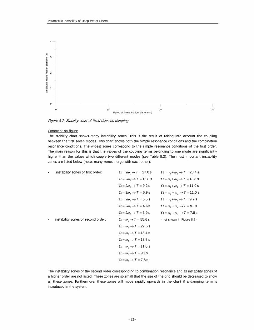
Parametric Instability of Deep-Water Risers
- 82 -
0 10 20 30Period of heave motion platform (s)
0
1
2
3
4
Ampl
itude
hea
ve m
otio
n pl
atfo
rm (
m)
Figure 8.7: Stability chart of fixed riser, no damping Comment on figure The stability chart shows many instability zones. This is the result of taking into account the coupling between the first seven modes. This chart shows both the simple resonance conditions and the combination resonance conditions. The widest zones correspond to the simple resonance conditions of the first order. The main reason for this is that the values of the coupling terms belonging to one mode are significantly higher than the values which couple two different modes (see Table 8.2). The most important instability zones are listed below (note: many zones merge with each other).
- instability zones of first order: 12 27.8TωΩ = → = s 1 2 28.4Tω ωΩ = + → = s
22 13.8TωΩ = → = s 1 3 13.8Tω ωΩ = + → = s
32 9.2TωΩ = → = s 1 4 11.0Tω ωΩ = + → = s
42 6.9TωΩ = → = s 2 3 11.0Tω ωΩ = + → = s
52 5.5TωΩ = → = s 1 5 9.2Tω ωΩ = + → = s
62 4.6TωΩ = → = s 2 4 9.1Tω ωΩ = + → = s
72 3.9TωΩ = → = s 3 4 7.8Tω ωΩ = + → = s
- instability zones of second order: 1 55.6TωΩ = → = s - not shown in Figure 8.7 -
2 27.6TωΩ = → = s
3 18.4TωΩ = → = s
4 13.8TωΩ = → = s
5 11.0TωΩ = → = s
6 9.1TωΩ = → = s
7 7.8TωΩ = → = s
The instability zones of the second order corresponding to combination resonance and all instability zones of a higher order are not listed. These zones are so small that the size of the grid should be decreased to show all these zones. Furthermore, these zones will move rapidly upwards in the chart if a damping term is introduced in the system.

Parametric Instability of Deep-Water Risers
- 83 -
8.3.2 System including linear damping coefficient Figure 8.7 shows all excitation periods at which parametric instability occurs if no damping is included in the model. The damping caused by the surrounding water leads to an extra term in the set of differential equations:
2 cos ( ) 0( )m m m mn n m m m
r f a
S tq q f q c qm m m
ω α ωΩ+ − + =
+ + ∑&& & 1, 2,...m n= [8.30]
in which c is the damping coefficient defined by expression [8.14]. This coefficient is proportional to the maximum value of the displacement amplitude ;maxnφ of the analysed modes.
Appendix G contains the values for the mode dependent parameter nα .
The system of equations including damping becomes:
1
7
21 11 17 1 18
271 7 77 7 714
0 .. 0 1 .. 0.. .. .. .. .. .. ..
0 .. 0 0 .. 1cos cos.. .. 0
( ) ( ).. .. .. .. .. .. ..
cos cos.. 0 ..( ) ( )
r f a r f a
r f a r f a
x
xS t S tf f cx
m m m m m m
S t S tf f cxm m m m m m
ω α ω
ω α ω
⎡ ⎤ ⎡⎢ ⎥ ⎢⎢ ⎥ ⎢⎢ ⎥ ⎢⎢ ⎥ ⎢
Ω Ω⎢ ⎥ ⎢− + −=⎢ ⎥ ⎢ + + + +⎢ ⎥⎢ ⎥⎢ ⎥ Ω Ω⎢ ⎥ − + −
+ + + +⎢ ⎥ ⎣⎣ ⎦
&
&
&
&
1
7
8
14
..
..
x
x
x
x
⎡ ⎤⎤⎢ ⎥⎥⎢ ⎥⎥⎢ ⎥⎥⎢ ⎥⎥⎢ ⎥⎥ ⋅ ⎢ ⎥⎥⎢ ⎥⎢ ⎥⎢ ⎥⎢ ⎥⎢ ⎥⎢ ⎥⎢ ⎥⎢ ⎥⎢ ⎥⎢ ⎥⎦ ⎣ ⎦
[8.31] The fixed riser configuration corresponds to the drilling and production stage. The following amplitudes and frequencies of the heave motion of the platform during these stages are assumed to be realistic: - period of the heave motion, T : 5 25− s - amplitude of the heave motion, A : 0 5− m Note: the maximum value of the amplitude ( 5A = m) is not based on research but this value is arbitrarily chosen to enable the analysis of parametric instability. The value for the damping coefficient c is gradually increased until all instability zones are located outside the area which is defined above. The stability chart which is finally obtained is shown in Figure 8.8.

Parametric Instability of Deep-Water Risers
- 84 -
0 40 80 120 160Time (s)
-0.8
-0.4
0
0.4
0.8
1.2
Tim
e fu
nctio
n (-
)
-2 -1 0 1 2 3
Horizontal deflection (m)
1200
800
400
0
Elev
atio
n of
ris
er (
m)
Figure 8.8: Stability chart of fixed riser, including damping (c=1.13) Comment on figure The shaded area in Figure 8.8 represents the instability zones which are merged resulting in one area.
The damping coefficient corresponding to the merged instability zone as shown in Figure 8.8 is equal to 1.13. According to Figure 8.8 the maximum deflection of the riser motion is expected for a heave motion of the platform with a period of 5.5s and amplitude of 5m. This combination is indicated in the stability chart with a black dot ( ). It is impossible to conclude from the stability chart which mode is excited for this heave motion, because the chart shows one large instable area without clear peaks.
8.3.3 Approximation of maximum amplitude horizontal riser displacement In this paragraph the system of equations which is given by equation [8.31] will be integrated numerically for the heave motion which is represented by the black dot in Figure 8.8. By obtaining the amplitudes of the time functions of the modes it is possible to estimate the maximum expected deflection of the 1500m fixed riser. Figure 8.9a: Time functions, mode 1 through mode 7 Figure 8.9b: Riser deflection at t=170s
area containing all realistic heave motions of platform
0 5 10 15 20 25 30Period of heave motion platform (s)
0
2
4
6
8
10
Ampl
itude
of
heav
e m
otio
n pl
atfo
rm (
m)

Parametric Instability of Deep-Water Risers
- 85 -
In Figure 8.9a the time functions ( )nq t are plotted as function of time for the value of the linear
damping coefficient c equal to 1.13. In Figure 8.9b the deflection of the riser is plotted at a moment when the deflection reaches its maximum value. From Figure 8.9a it can be concluded that mode 5 (black line) is excited. This conclusion is drawn because of the frequency of the time function, which is equal to the natural frequency of the fifth mode. The other modes are characterized by a relatively large amplitude of the time function. The reason for this is the coupling between the modes. Consequently, the shape of the riser deflection as shown in Figure 8.9b is not equal to the shape of mode 5 but it is a combination of the first seven modes. One of the characteristics of this shape is the relatively large deflection at the lower part of the riser. Here the value of the static tension is small, so the contribution of the additional tension is relatively large. The maximum riser displacement is estimated using Figure 8.9b. This figure shows a maximum riser displacement of 2.75m.
8.3.4 Stresses in riser due to parametric instability In this paragraph the bending stresses and the additional tensile stresses due to the parametric instability are calculated and compared with the yield stress of steel. For more information about the stresses in the riser see paragraph 8.2.4. To obtain the maximum value of the bending moment the riser shape which is shown in Figure 8.9b is used. For the bending moment yields the following equation:
2
2
( )( ) d w zM z EIdz
= − [8.32]
in which ( )w z is the deflection of the riser as shown in Figure 8.9b.
A short calculation shows that ( )M z reaches its maximum value at 1410z = m:
max (1410 m) 19.4M M= = kNm
According to equation [8.20] the maximum bending stress in the riser becomes:
b;max 16σ = MPa
The additional tensile stress is constant along the riser. Substituting the expression for S given by equation [8.7] into equation [8.21] the additional tensile stress is equal to:
vertt;add 65
s
A kA
σ⋅
= = MPa
The yield stress yσ of steel is around 360 MPa.

Parametric Instability of Deep-Water Risers
- 86 -
These results imply that the additional tensile stress induced by time varying tension force is much larger than the stress due to bending. The total increase of stress in the critical cross section of the riser is approximately 25% of the yield stress.
8.4 Application: free hanging riser (Model C) 8.4.1 Stability chart of system without damping The set of equations for this riser configuration is derived in paragraph 6.3.4 and is repeated below:
( )2 max cos0
( ) m m m mn nnr f a
S tq q f q
m m mω
⋅ Ω+ − =
+ + ∑&& , 1, 2, 3....,m n= [8.33]
( )0
2
0
1L
m n
mn L
m
z L dzf
dz
φ φ
φ
′ ′− ⋅ ⋅= −∫
∫ [8.34]
To analyse this system the coupling factors mnf should be determined. A FORTRAN program has
been written that calculates these factors based on the mode shapes determined in Chapter 5. The results for the first eight normal modes are shown in Table 8.3.
1φ 2φ 3φ 4φ 5φ 6φ 7φ 8φ
1 0.0638ω =rad/s
2 0.1465ω =rad/s
3 0.2303ω =rad/s
4 0.3163ω =rad/s
5 0.4057ω =rad/s
6 0.4989ω =rad/s
7 0.5951ω =rad/s
8 0.6938ω =rad/s
11 -6.44E-7f =
21 -5.71E-9f =
31 2.37E-9f = +
41 -1.11E-8f =
51 7.61E-9f = +
61 -1.47E-8f =
71 1.18E-8f = +
81 -1.69E-8f =
12 -2.51E-9f =
22 -3.40E-6f =
32 -8.47E-9f =
42 2.07E-8f = +
52 -2.46E-9f =
62 3.22E-8f = +
72 -8.08E-9f =
82 3.72E-8f = +
13 0.74E-9f = +
23 -5.96E-9f =
33 8.36E-6f = −
43 5.71E-8f = +
53 1.27E-7f = +
63 8.86E-8f = +
73 1.37E-7f = +
83 7.23E-8f = +
14 -3.11E-9f =
24 2.50E-9f = +
34 5.16E-8f = +
44 1.56E-5f = −
54 3.18E-7f = +
64 4.19E-7f = +
74 3.43E-7f = +
84 3.97E-7f = +
15 2.24E-9f = +
25 -1.64E-9f =
35 1.21E-7f = +
45 3.34E-7f = +
55 2.52E-5f = −
65 8.65E-7f = +
75 9.83E-7f = +
85 8.26E-7f = +
16 -4.81E-9f =
26 2.39E-8f = +
36 9.37E-8f = +
46 4.90E-7f = +
56 9.64E-7f = +
66 3.77E-5f = −
76 1.82E-6f = +
86 1.90E-6f = +
17 4.34E-9f = +
27 6.77E-9f = −
37 1.64E-7f = +
47 4.72E-7f = +
57 1.24E-6f = +
67 2.05E-6f = +
77 5.29E-5f = −
87 3.25E-6f = +
18 -7.02E-9f =
28 3.51E-8f = +
38 9.70E-8f = +
48 5.89E-7f = +
58 1.17E-6f = +
68 2.41E-6f = +
78 3.65E-6f = +
88 7.12E-5f = −
Table 8.3: Coupling factors of first 8 normal mode shapes [m-2]

Parametric Instability of Deep-Water Risers
- 87 -
From Table 8.3 it can be concluded that the coupling factors between the different mode shapes are surprisingly small: in most cases at least 100 times smaller than the factors mmf (indicated by
the gray markings). The explanation for these small coupling factors is found in the decrease of influence of the bending stiffness on the riser behaviour for long risers. A riser of this length behaves more like a cable than a pre-stressed beam. If the bending stiffness is left out of the system the normal mode shapes are the eigenfunctions of the problem:
2( )( ) ( ) ( ) 0n
r f a n nd zd T z m m m z
dz dzφ
ω φ+ + + ⋅ ⋅ = [8.35]
Multiplying equation [8.35] by mφ and integrating the result from 0z = to z L= , gives:
2
0 0
d ( )d ( ) ( ) ( ) ( ) ( ) 0d d
L Ln
m r f a n n mz
T z z dz m m m z z dzz z
φφ ω φ φ+ + + ⋅ ⋅ =∫ ∫ [8.36]
Using the orthogonality condition of the normal modes the integral 0
( ) ( )L
n mz z dzφ φ∫ is equal to
zero for m n≠ . From equation [8.36] the following is concluded:
0
d ( )d ( ) ( ) 0d d
Ln
mz
T z z dzz z
φφ =∫ for m n≠ [8.37]
It follows from equation [6.21] in Chapter 6 that the coupling factors mnf which are shown in
Table 8.3 are proportional to the following expression:
0
( )( ) ( )
Ln
mn md zdf S z z dz
dz dzφ
φ∫ [8.39]
This implies that if ( )T z and ( )S z have the same shape the coupling factors become zero for
m n≠ . In this case both forces are linear in z -direction with the maximum value at the riser top and the minimum value equal to zero at the riser tip. An explanation for the fact that the values of mnf are not exactly zero is the inaccuracy of the FORTRAN program that is used to compute
these coupling factors and a small influence of the bending stiffness which is still be present. In this paragraph the riser configuration is assumed to be entirely uncoupled. Because of this the calculation time will be significantly shortened. In the next paragraph the stability chart will be constructed for the uncoupled set of equations and the coupled set of equations. In this paragraph a damping term is included in the model to make a first estimation of the riser displacements.

Parametric Instability of Deep-Water Risers
- 88 -
The expression of the time varying component of the tension force, S , is derived in Appendix A. The riser is assumed to be a rigid body. For a free hanging riser configuration the following expression holds:
2max ( )s sS A A Lρ= ⋅Ω ⋅ [8.39]
where A is the amplitude of the heave motion of the platform [m] Substituting equation [8.39] into equation [8.33] shows that the system of equations [8.33] contains two variables: the amplitude of the heave motion A and the radial frequency of this motion Ω . The application of the Floquet theory for this case is the same as for the simply supported riser with constant tension, see paragraph 8.2.1. The results are shown in a stability chart; see Figure 8.10. This chart shows the combinations of A and T ( )2π= Ω for which this
riser configuration behaves unstable if no damping is present.
0 5 10 15 20 25Period of heave motion platform (s)
0
2
4
6
8
10
Ampl
itude
hea
ve m
otio
n pl
atfo
rm (
m)
Figure 8.10: Stability chart of free hanging riser, no damping Comment on figure The instability zones corresponding to normal mode 9 and higher are not constructed. These zones are located in the domain of the excitation period smaller than 4s. It is assumed that the frequency of the heave motion of the platform will not reach such high values. Conversely, the primary instability zone corresponding to the first normal mode occurs for a very low value of the frequency of the heave motion. The stability chart in Figure 8.10 contains 7 primary instability zones. No secondary instabilities zones are constructed because these are very small. Furthermore if a damping term is introduced these zones moves rapidly upwards. The excitation periods which correspond to the primary instabilities are listed below:
22 21.5TωΩ = → = s 62 6.3TωΩ = → = s
32 13.7TωΩ = → = s 72 5.3TωΩ = → = s
42 9.9TωΩ = → = s 82 4.5TωΩ = → = s
52 7.7TωΩ = → = s

Parametric Instability of Deep-Water Risers
- 89 -
8.4.2 System including linear damping coefficient Uncoupled system of equations In Figure 8.10 all excitation periods are shown at which parametric instability occurs if no damping is included in the model. In reality the riser is surrounded by fluid. As derived in paragraph 8.2.2 for the simplified riser configuration, the damping caused by the surrounding water leads to an extra term in the set of differential equations:
2 max cos0
( )n n n nn n n n nr f a
S tq q f q c q
m m mω α ω
Ω+ − + =
+ +&& & [8.40]
in which c is the damping coefficient defined by expression [8.14]. Appendix G contains the values for the mode dependent parameter nα .
To make an estimation of the maximum lateral riser displacement an area should be defined in the stability chart which contains the heave motions which can be expected with a certain probability during this stage. The free hanging riser configuration corresponds to the installation stage. The duration of this process is relatively short. This implies that the amplitude of the heave motion which is normative for this configuration is smaller than for the fixed riser configurations. For this case the following area in the stability chart is assumed to be realistic: - period of the heave motion, T : 5 25− s - amplitude of the heave motion, A : 0 3− m The value for the damping coefficient is gradually increased until all instability zones are located outside the area which is defined above. The stability chart is shown in Figure 8.11. Figure 8.11: Stability chart for uncoupled system, including damping (c=0.67)
area containing all realistic heave motions of platform
0 5 10 15 20 25Period of heave motion of platform (s)
0
2
4
6
8
10
Ampl
itude
hea
ve m
otio
n pl
atfo
rm (
m)

Parametric Instability of Deep-Water Risers
- 90 -
Comment on figure: The instability zones corresponding to the first normal modes are located outside the range of the stability chart. This is the result of the fact that the time varying tension force depends on the frequency of the
heave motion: 2max ( )s sS A A Lρ= ⋅Ω ⋅ . Because of the small magnitude of the time varying tension force
related to relatively large periods ( 2max 1S T ) these instability zones are of minor importance.
The damping coefficient required to construct the stability chart as shown in Figure 8.11 is equal to 0.67. According to this figure the maximum deflection of the riser motion is expected for a heave motion of the platform with a period of 5s and amplitude of 3m. This combination is indicated in the stability chart with a black dot ( ). The seventh normal mode is excited. Coupled system of equations In Figure 8.12 the stability chart is obtained for the case that coupling between the modes is taken into account. This coupling of the differential equations leads to extra resonance conditions: combination resonances. Figure 8.12: Stability chart for coupled system, including damping (c=0.67) Comment on figure Figure 8.12 shows exactly the same results as Figure 8.11 for the damping coefficient equal to 0.67. The assumption that the system can be considered as uncoupled is correct.
8.4.3 Approximation of maximum amplitude horizontal riser displacement In this paragraph the system of equations which is given by equation [8.43] will be numerically integrated for the heave motion which is represented with the black dot in Figure 8.12. By obtaining the amplitudes of the time functions of the modes it is possible to estimate the maximum expected deflection of the 1500m fixed riser.
area containing all realistic heave motions of platform
0 5 10 15 20 25Period of heave motion of platform (s)
0
2
4
6
8
10
Ampl
itude
hea
ve m
otio
n pl
atfo
rm (
m)

Parametric Instability of Deep-Water Risers
- 91 -
0 40 80 120 160Time (s)
-4
-2
0
2
4
6
Tim
e fu
nctio
n (-
)
-1.5 -1 -0.5 0 0.5 1
Horizontal deflection (m)
1500
1000
500
0
Elev
atio
n of
ris
er (
m)
In Figure 8.12a the time functions ( )nq t are plotted as function of time for the value of the linear
damping coefficient equal to 0.67. In Figure 8.12b the deflection of the riser is plotted at a moment when the deflection reaches its maximum value. Figure 8.12a: Time functions, mode 1 through mode 8 Figure 8.12b: Riser deflection at t=155s In Figure 8.12a the black line shows the time function of mode 7. The boundary of the instability zone corresponding to this mode touches the point in the stability chart representing this heave motion (black dot in Figure 8.12). The other modes are not excited so these time functions go to zero. Figure 8.12b shows that the value of the maximum deflection of the riser is around 1.3m. The shape of the deflection corresponds to the shape of mode 7.
8.4.4 Stresses in riser due to parametric instability In this paragraph the bending stresses and the additional tensile stresses due to the parametric instability are calculated and compared with the yield stress of steel. Hence it is possible to gain more insight in the contribution of this parametric excitation to the stresses in the riser. In Chapter 5 the normal modes of this riser configuration are determined. The results for the seventh mode are used to obtain the maximum value of the bending moment in the riser corresponding to a maximum riser deflection of 1.3m. ( )M z reaches its maximum value at
1450z = m:
max (1450 m) 15M M= = kNm
Using equation [8.20] the maximum bending stress in the riser becomes:
b;max 24σ = MPa
The additional tensile stress reaches its maximum value at the riser top. Substituting the expression for ( )S z given by equation [8.39] into equation [8.21] the additional tensile stress is
equal to:

Parametric Instability of Deep-Water Risers
- 92 -
2maxt;add;max 56s
s
SA L
Aσ ρ= = ⋅Ω ⋅ ⋅ = MPa
The yield stress yσ of steel is around 360 MPa.
These results imply that the additional tensile stress induced by time varying tension force is twice as large as the stress due to bending. The total increase of stress in the critical cross section of the riser (riser top) is approximately 20% of the yield stress.

Parametric Instability of Deep-Water Risers
- 93 -
9 Analysis of different riser lengths
9.1 Introduction In this chapter the parametric instability is analysed for risers with a different riser length. In section 9.2 the free hanging riser is analysed for a length of 3000m. This huge riser length is not purely a theoretical case; nowadays, drilling in such deep water is already performed. Section 9.3 deals with the case of a water intake riser having a length of 100m. This riser is a free hanging pipe which is used for pumping up cold water. This water is used as cooling water for the process of liquefying natural gas on a plant on a barge. The results of this chapter along with the results of the previous chapter should make clear how the riser length influences the response of the riser to the heave motion of the platform.
9.2 Parametric excitation of 3000m risers
9.2.1 General In this section risers in very deep water are analyzed. These risers have a length up to 3000m. In paragraph 9.2.2 the instability due to the parametric excitation for a free hanging riser configuration is determined. The fixed riser used for the drilling operation is not considered in this section. The reason for this is the design of this type of risers in very deep water. If the same riser is used for drilling as in the previous chapters the tensile stresses at the upper part of the riser will reach such high values that the yield stress is exceeded even without the incorporation of the parametric excitation into the model. To prevent this kind of failure buoyancy cans are used. These cans provide an extra buoyancy force along the riser in order to decrease the tensile stresses in the riser. These additional units change the system in such a way that the used model can not be applied for this kind of risers. Conversely, production risers have a smaller cross sectional area of the steel wall, so the tension in the riser top will not exceed the yield stress. In the next paragraph the free hanging production riser is further analysed. The fixed production riser is not analysed to limit the number of cases just as in the previous chapters.
9.2.2 Free hanging riser in very deep water The cross section of the riser is kept the same as for the 1500m riser. Due to the modification of the length the natural frequencies of this system will differ from the frequencies obtained in Chapter 5. The spectrum of natural frequencies is denser. This implies that more normal modes should be taken into account to obtain the stability chart. The calculation time will not increase

Parametric Instability of Deep-Water Risers
- 94 -
very much because the system of equations is decoupled. On the basis of five steps the stability of this riser configuration is analyzed: - Define the equation of motion and determine the natural frequencies of the system in which
the platform motions are assumed to be zero. - Determine the system of first order equations which is valid for the system including the
parametric excitation. - Construct the stability chart for the case without damping. - Incorporate the linear damping into the model and obtain the upper bound of the maximum
lateral displacement. - Calculate the bending stresses and additional tensile stresses in the riser which are induced
by the parametric excitation. The outlined procedure is the same as the one used for the riser configurations with a length of 1500m. But in this chapter the explanation is much shorter. Natural frequencies To obtain the natural frequencies of the system the time varying component is not included into the model. The resulting equation of motion is reduced to a fourth-order linear partial differential equation whose coefficients are independent of time. To integrate this differential equation the same FORTRAN program is used as mentioned in Section 5.3. The result of the FORTRAN program for the free hanging riser of 3000m is shown in Figure 9.1. In this figure the amplitudes of the horizontal displacement ˆ ( , )w z ω are plotted as function of the
excitation frequency for three elevations, 500 m, 2000 m, 3000 mz = . The excitation frequencies
for which the amplitudes reach a peak value correspond to the natural frequencies of the system. In Table 9.1 the values of the first natural frequencies are listed. Figure 9.1: Frequency response function for 3000m free hanging riser at three elevations
0 0.2 0.4 0.6 0.8 1excitation frequency (rad/s)
ampl
itude
of
riser
def
lect
ion 500 mz =
2000 mz =
3000 mz =
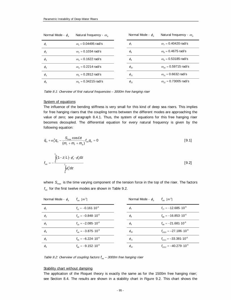
Parametric Instability of Deep-Water Risers
- 95 -
Table 9.1: Overview of first natural frequencies – 3000m free hanging riser System of equations The influence of the bending stiffness is very small for this kind of deep sea risers. This implies for free hanging risers that the coupling terms between the different modes are approaching the value of zero; see paragraph 8.4.1. Thus, the system of equations for this free hanging riser becomes decoupled. The differential equation for every natural frequency is given by the following equation:
2 max cos0
( )n n n nn nr f a
S tq q f q
m m mω
Ω+ − =
+ +&& [9.1]
( )0
2
0
1L
n n
nn L
n
z L dzf
dz
φ φ
φ
′ ′− ⋅ ⋅= −∫
∫ [9.2]
where maxS is the time varying component of the tension force in the top of the riser. The factors
nnf for the first twelve modes are shown in Table 9.2.
Table 9.2: Overview of coupling factors nnf – 3000m free hanging riser
Stability chart without damping The application of the Floquet theory is exactly the same as for the 1500m free hanging riser; see Section 8.4. The results are shown in a stability chart in Figure 9.2. This chart shows the
Normal Mode - nφ Natural frequency - nω
1φ 1 0.04495ω = rad/s
2φ 2 0.1034ω = rad/s
3φ 3 0.1622ω = rad/s
5φ 4 0.2214ω = rad/s
4φ 5 0.2812ω = rad/s
6φ 6 0.34215ω = rad/s
Normal Mode - nφ Natural frequency - nω
7φ 7 0.40420ω = rad/s
8φ 8 0.4675ω = rad/s
9φ 9 0.53185ω = rad/s
10φ 10 0.59715ω = rad/s
11φ 11 0.6632ω = rad/s
12φ 12 0.73005ω = rad/s
Normal Mode - nφ nnf [m-2]
1φ -611 0.161 10f = − ⋅
2φ -622 0.848 10f = − ⋅
3φ -633 2.085 10f = − ⋅
4φ -644 3.875 10f = − ⋅
5φ -655 6.224 10f = − ⋅
6φ -666 9.152 10f = − ⋅
Normal Mode - nφ nnf [m-2]
7φ -677 12.685 10f = − ⋅
8φ -688 16.853 10f = − ⋅
9φ -699 21.681 10f = − ⋅
10φ -61010 27.186 10f = − ⋅
11φ -61111 33.381 10f = − ⋅
12φ -61212 40.279 10f = − ⋅

Parametric Instability of Deep-Water Risers
- 96 -
combinations of the amplitude of the heave motion A and period this motion T for which this riser configuration behaves unstable. No damping is included in the model.
0 5 10 15 20 25 30Period of heave motion platform (s)
0
2
4
6
8
10
Apm
litud
e he
ave
mot
ion
plat
form
(m
)
Figure 9.2: Stability chart for 3000m free hanging riser, no damping The stability chart is very similar to the stability chart which is obtained for the 1500m free hanging riser. The main difference is that the instability zones are located closer to each other. The reason for this is that the spectrum of natural frequencies for this very long riser is denser. Upper bound of maximum lateral displacement The damping caused by the surrounding water leads to an extra term in the set of differential equations. The differential equation for every natural frequency is given by:
2 max cos0
( )n n n nn n n n nr f a
S tq q f q c q
m m mω ω α
Ω+ − + =
+ +&& & [9.3]
in which c is the damping coefficient defined by expression [8.14]. This coefficient is proportional to the maximum value of the displacement amplitude of the analysed mode ( ,maxnφ ).
Appendix G contains the values for the mode dependent parameter nα .
The value for the linear damping coefficient is gradually increased until all instability zones are located outside a predefined area. This area contains all realistic combinations of the amplitude and the period of the heave motion which can occur. The stability chart is shown in Figure 9.3.

Parametric Instability of Deep-Water Risers
- 97 -
0 40 80 120 160Time (t)
-2
-1
0
1
2
Tim
e fu
nctio
n (-
)
Figure 9.3: Stability chart for 3000m free hanging riser, including damping (c=0.77) The required damping coefficient to construct the stability chart as shown in Figure 9.3 is equal to 0.77. According to this figure the maximum amplitude of the riser motion is expected for a heave motion of the platform with a period of 5s and amplitude of 3m. This combination is indicated in the stability chart with a black dot ( ). This point in the stability chart is on the transition curve separating stability from instability corresponding to the tenth mode. For this heave motion the time functions of all modes will decrease in time to zero except the time function of mode 10. This time function is plotted in Figure 9.4. Figure 9.4: Time function of mode 10 The amplitude of this time function is used to calculate the maximum expected riser displacement using the following formula:
10;max 10 102( )ˆ ˆˆ 1.5r f a
w o d
m m mw q c q
D Cφ
ρ+ +
= ⋅ = ⋅ ⋅ ≈ m
Area containing all realistic heave motions of platform
0 5 10 15 20 25 30Period of heave motion platform (s)
0
2
4
6
8
10
Ampl
itude
hea
ve m
otio
n pl
atfo
rm (
m)

Parametric Instability of Deep-Water Risers
- 98 -
Stresses due to parametric instability The bending stresses and the additional tensile stresses due to the parametric instability are calculated and compared with the yield stress of steel. Hence it is possible to gain more insight in the contribution of this parametric excitation to the stresses in the riser. The expressions to calculate the maximum bending stress and the additional tensile stress in a cross section of the riser are given in Chapter 8. The shape of the deflection corresponding to the tenth mode is used to obtain the maximum value of the bending moment in the riser corresponding to a maximum riser deflection of 1.5m.
( )M z reaches its maximum value at 2950z = m:
max (2950 m) 17M M= = kNm
Using equation [8.20] the maximum bending stress in the riser becomes:
b;max 28σ = MPa
The additional tensile stress reaches its maximum value at the riser top. Using the expression for
maxS given by equation [8.39] the additional tensile stress is equal to:
2maxt;add;max 112s
s
SA L
Aσ ρ= = ⋅Ω ⋅ ⋅ = MPa
The yield stress yσ of steel is around 360 MPa. These results imply that the additional tensile
stress induced by time varying tension force is of much more importance than the stress due to bending. The total increase of stress in the critical cross section of the riser (riser top) is approximately 35% of the yield stress.
9.3 Parametric excitation of 100m water intake riser This section deals with the case of a water intake riser having a length of 100m. The cross section of this riser is much larger than the one of a production riser. Due to the modification of the cross section and the length of the pipe the spectrum of the natural frequencies of this system will be less dense compared to spectra of the other two configurations. This implies that less normal modes have to be taken into account to obtain the stability chart. Nevertheless, the calculation time could increase because the system of equations is coupled. On the basis of the same five steps as used in the previous section the stability of this riser configuration is analyzed. Natural frequencies To obtain the natural frequencies of the system the time varying component is not included into the model. To integrate the resulting differential equation a FORTRAN program is used which is mentioned in Chapter 5.3. The result of the FORTRAN program for the free hanging riser of 100m is shown in Figure 9.5. In this figure the amplitudes of the horizontal displacement ˆ ( , )w z ω are

Parametric Instability of Deep-Water Risers
- 99 -
plotted as function of the excitation frequency for three elevations, 50z = m and 100z = m. The excitation frequencies for which the amplitudes reach a peak value correspond to the natural frequencies of the system. In Table 9.3 the values of the first natural frequencies are listed. Figure 9.5: Frequency response function for the water intake riser at two elevations
Table 9.3: First natural frequencies – water intake riser System of equations The influence of the bending stiffness is not negligible for water intake risers because of the small length and the large diameter. Thus, the system of equations for this riser configuration is coupled. The system of differential equations is given by the following equations:
2 max cos( ) 0
( )m m m mn nr f a
S tq q f q
m m mω
Ω+ − =
+ + ∑&& , 1, 2,...m n= [9.4]
( )0
2
0
1L
m n
mn L
m
z L dzf
dz
φ φ
φ
′ ′− ⋅ ⋅= −∫
∫ [9.5]
where maxS is the time varying component of the tension force in the top of the riser. The
coupling factors mnf for the first three modes are shown in Table 9.4.
Normal Mode - nφ Natural frequency - nω
1φ 1 0.4479ω = rad/s
2φ 2 2.474ω = rad/s
3φ 3 6.823ω = rad/s
0 2 4 6 8 10Excitation frequency (rad/s)
Ampl
itude
of ris
er d
efle
ctio
n 50 mz =
100 mz =

Parametric Instability of Deep-Water Risers
- 100 -
1φ
1 0.4479ω = rad/s 2φ
2 2.474ω = rad/s 3φ
3 6.823ω = rad/s
-511 15.74 10f = − ⋅ m-2 -5
21 4.41 10f = − ⋅ m-2 -531 10.21 10f = + ⋅ m-2
-512 4.35 10f = − ⋅ m-2 -5
22 87.11 10f = − ⋅ m-2 -532 17.30 10f = + ⋅ m-2
-513 10.16 10f = + ⋅ m-2 -5
23 17.44 10f = + ⋅ m-2 -533 250.38 10f = − ⋅ m-2
Table 9.4: Overview of coupling factors mnf – water intake riser
Stability chart without damping The application of the Floquet theory is exactly the same as for the 1500m free hanging riser; see Section 8.4. The results are shown in a stability chart; see Figure 9.6. This chart shows the combinations of the amplitude of the heave motion A and the period of this motion T for which this riser configuration behaves unstable. No damping is included in the model.
0 5 10 15 20 25Period of heave motion platform (s)
0
2
4
6
8
10
Ampl
itude
hea
ve m
otio
n pl
atfo
rm (
m)
Figure 9.6: Stability chart for water intake riser, no damping The stability chart shows one instability zone which is of importance: an excitation period near 7s. This zone corresponds to the primary instability zone of the first mode. All other zones are located in the domain of the excitation period smaller than 3s. It is assumed that the frequency of the heave motion of the platform will not reach such high values. Upper bound of maximum lateral displacement The damping caused by the surrounding water leads to an extra term in the set of differential equations. The system of equations reads:
2 max cos( ) 0
( )m m m mn n m m mr f a
S tq q f q c q
m m mω α ω
Ω+ − + =
+ + ∑&& & , 1, 2,...m n= [9.6]
in which c is the damping coefficient defined by expression [8.14].

Parametric Instability of Deep-Water Risers
- 101 -
0 40 80 120Time (s)
-3
-2
-1
0
1
2
3
Tim
e fu
nctio
n (-
)
The value for the damping coefficient is gradually increased until the primary instability zone of the first mode is located outside the predefined area. This area contains all realistic combinations of the amplitude and the period of the heave motion which can occur. The water intake riser is used in the production stage in contrast to the free hanging risers of 1500m and 3000m. This justifies that the maximum expected amplitude of the heave motion is equal to 5m; the same value as for the fixed riser configuration. The stability chart is shown in Figure 9.7. Figure 9.7: Stability chart for water intake riser, including damping (c=0.07) The required damping coefficient to construct the stability chart as shown in Figure 9.7 is equal to 0.07. According to this figure the maximum amplitude of the riser motion is expected for a heave motion of the platform with a period of 7s and amplitude of 5m. This combination is indicated in the stability chart with a black dot ( ). This point in the stability chart is on the transition curve separating stability from instability corresponding to the first mode. Performing the time domain analysis the time functions of all three modes are obtained; see Figure 9.8. Figure 9.8: Time functions, mode 1 through mode 3
area containing all realistic heave motions of platform
0 5 10 15 20 25Period of heave motion platform (s)
0
2
4
6
8
10
Ampl
itude
hea
ve m
otio
n pl
atfo
rm (
m)

Parametric Instability of Deep-Water Risers
- 102 -
The black line shows the time function of mode 1. The amplitude of this time function is used to calculate the maximum expected riser displacement using the following formula:
1;max 10 12( )ˆ ˆˆ 1.0r f a
w o d
m m mw q c q
D Cφ
ρ+ +
= ⋅ = ⋅ ⋅ ≈ m
Stresses due to parametric instability The bending stresses and the additional tensile stresses due to the parametric instability are calculated and compared with the yield stress of steel. Hence it is possible to gain more insight in the contribution of this parametric excitation to the stresses in the riser. The expressions to calculate the maximum bending stress and the additional tensile stress in a cross section of the riser are given in Chapter 8. The shape of the deflection corresponding to the first mode is used to obtain the maximum value of the bending moment in the riser corresponding to a maximum riser deflection of 1.0m.
( )M z reaches its maximum value at the riser top: 0z = m:
max (0 m) 1.1M M= = kNm
The maximum bending stress in the riser becomes:
b;max 38σ = MPa
The additional tensile stress reaches its maximum value at the riser top. Using the expression for
maxS given by equation [8.39] the additional tensile stress is equal to:
2maxt;add;max 3s
s
SA L
Aσ ρ= = ⋅Ω ⋅ ⋅ = MPa
The yield stress yσ of steel is around 360 MPa.
These results show that the additional tensile stress induced by time varying tension force is very small because of the small weight of the riser. The total increase of stress in the critical cross section of the riser (riser top) is approximately 10% of the yield stress.

Parametric Instability of Deep-Water Risers
- 103 -
10 Conclusions and recommendations
10.1 Conclusions This section contains the conclusions of this study. These conclusions arise from the objective which is stated in Chapter 2 and the results obtained in Part B and Part C. The main objective is repeated below: “The objective of this study is to gain more insight in the phenomenon called parametric instability. The focus is on the occurrence of instability for deep-water risers induced by the variation of the effective tension in time.” In order to analyse the dynamic stability of the riser due to a time varying tension force the Floquet Theory is used. This method is found to be the most suitable method to deal with this parametrically excited system. A program, written in FORTRAN, applies this theory to construct a stability chart for different riser configurations. This chart shows the combinations of magnitude and period of the time varying force for which the system behaves unstable. Before applying the Floquet Theory the program determines the natural frequencies and normal modes of a closely related system, calculates the coupling factors between these modes and calculates the mode dependent linear damping coefficients. The conclusions from this analysis are listed below: The riser is a continuous system which has an infinite number of natural frequencies and
corresponding normal modes. By applying the Galerkin’s Method the system is described by an infinite set of differential equations.
This set of equations is coupled by mode dependent coupling factors. For some cases the set of equations becomes decoupled. Two cases can be distinguished:
- Theoretical case: a beam simply supported at both ends with a static and dynamic tension which is constant along the z-axis.
- Practical case: a riser for which the bending stiffness can be neglected compared to the influence of the tension force; riser modelled as a cable. Furthermore, the shape along the z-axis of the static tension and the dynamic tension should be the same. These two conditions are fulfilled in case of a long free hanging riser in deep water.
The spectrum of natural frequencies ( ; 1, 2,....)n nω = for long risers is very dense. This leads
to many resonance conditions. The resonance conditions are defined by the following expression:

Parametric Instability of Deep-Water Risers
- 104 -
m np ω ω⋅Ω = ±
in which p is an integer. The absolute value of p defines the order of the instability zone.
One speaks of simple resonance when m n= . Combination resonance occurs when m n≠ . The boundaries between stability and instability in the neighbourhood of these resonance
conditions can be obtained by several methods. The Floquet Theory is very straightforward if the drag force is linearized. For a nonlinear analysis this method cannot be applied.
The primary instability zones are of much more importance than the secondary instability zones. These secondary zones are very narrow in the stability charts and if a linear damping term is introduced these zones become rapidly smaller.
The values of the coupling factors are the highest for adjacent modes. The highest value for every mode is reached for the coupling factor mmf . This implies that simple resonance exerts
greater influence on the stability of the riser than combination resonance. On the boundary of the stability zones the motion of the riser is periodic. This property can
be used to make a first approximation of the expected maximum riser displacement for a certain heave motion of the platform. Even for the largest expected heave motion the horizontal riser displacements will remain relatively small. The largest displacement is found for the fixed riser configuration: a heave motion of 5m amplitude and a period of 5.5s will cause a maximum horizontal riser displacement of 2.75m.
The bending stresses due the riser deflection are small compared to the yield stress of steel. The additional tensile stresses can become relatively large especially for risers in very deep
water (3000m). The reason for this is the large value of the mass of the riser. The objective of this study which is repeated at the beginning of this section is not complete. The objective as stated in Chapter 2 contains an additional question concerning the fixed riser configuration: “What is the influence of the tensioner system, modelled as soft springs, on the occurrence of parametric instability during the drilling operation and the production stage?” The answer to this question is found by varying the spring coefficient k of the soft springs that represent the tensioner system. In the previous chapters a relative vertical motion of the platform of 1m causes an additional tension force in the riser which is equal to 10% of the tension force in the riser top. In this analysis this relation is varied in the range of 5% through 15%. The spring coefficient does not significantly influence the natural frequencies and normal modes of the fixed riser. So in the stability analysis the time varying component of the tension force S is proportional to the value of the spring coefficient k . For several values of k the stability of the system is analysed by making use of the program, written in FORTRAN, that applies the Floquet theory. The approximation of the maximum expected horizontal riser displacement which depends on the value of the linear damping coefficient is shown as a function of the spring coefficient in Figure 10.1. These results are based on maximum amplitude of the heave motion equal to 5m and excitation period between 5s and 25s. These are the same values as used in Chapter 8 and Chapter 9.

Parametric Instability of Deep-Water Risers
- 105 -
0.025 0.05 0.075 0.1 0.125 0.15 0.175*T(0) Spring coefficient (N/m)
0
1
2
3
4
5
Mam
imum
hor
izon
tal d
ispl
acem
ent
(m)
Figure 10.1: Maximum horizontal riser displacement as function of vertical spring coefficient As a consequence from Figure 10.1 the following can be concluded: In this case, where the drag force is introduced as a linear term in the equation of motion,
the relation between the spring coefficient and the displacements of the riser is linear. A spring coefficient which is 2 times smaller, will lead to a decrease of the maximum
expected amplitude of the horizontal riser deflection of about 1.5m. This can be realized by increasing the total volume of air pressure vessels by a factor 2.
10.2 Recommendations In this section the recommendations are listed concerning items which could be further analyzed or improved to gain more insight in the phenomenon of parametric instability applied to marine risers. The Floquet Theory is only applicable for linear damping. In reality the drag force is a
nonlinear term. Solving the equation of motion including the nonlinear damping term in the time domain will give useful information about the maximum riser displacements which can be expected if the system behaves unstable. The most eminent difference of the solution in the time domain between linear damping and nonlinear damping is as follows: in case of linear damping the riser displacements will exponentially increase in time if the system is unstable. In case of nonlinear damping the displacements will reach an equilibrium value. This value can be compared with the approximation of the maximum riser displacements which are calculated on the basis of the linear damping coefficient c . In case of stability the riser displacements in the solutions with linear damping and with nonlinear damping will both finally diminish to zero.
In this study it is assumed that heave of the platform can be reduced to one harmonic motion. In reality the heave of the platform is characterized by a random process. It will be useful to analyse the stability of the riser in case of two parametric excitations. Finally the stability should be analyzed for a random vibration of the platform. Due to the nonlinearity in the system, superposition of the responses due to the excitations is not possible. Therefore

Parametric Instability of Deep-Water Risers
- 106 -
the behaviour as a result of the simultaneous action of these motions on the riser should be studied.
Based on the previous recommendation, it is interesting to combine a parametric excitation with a forcing excitation. Forcing excitations are introduced by horizontal platform oscillations and direct wave loading on the riser. Due to the nonlinearity in the system, simple superposition of the dynamic moment and strain is not possible.
In this study little attention is paid to the probability of a certain heave motion of the platform. In the stability charts an area is defined representing all realistic combinations of amplitude and period of the heave motion of the platform. To gain a better understanding of the role of parametric instability in the lifetime of a riser structure the long-term distribution of the heave spectrum should be incorporated.

Parametric Instability of Deep-Water Risers
- 107 -
References [1] Verkuylen RJ, ‘Water Intake Riser Analysis’, Master Thesis TU Delft, Shell Technology EP;
Rijswijk, April 2001 [2] Brockett Roger W, ‘Finite Dimensional Linear Systems’, John Wiley and Sons; New York,
1979 [3] Nayfeh AH and Mook DT, ‘Nonlinear Oscillations’, John Wiley and Sons; New York, 1970 [4] Yakubovich VA and Starzhinskii VM, ‘Linear Differential Equations with Periodic
Coefficients 2’, Wiley and Sons; New York, 1975 [5] Nayfeh AH and Mook DT, ‘Parametric Excitations of Linear Systems having many Degrees
of Freedom’, Journal of Acoustical Society of America; August 1977 [6] Friedmann P, Hammond CE and Woo TH, ‘Efficient Numerical Treatment of Periodic
Systems with Application to Stability Problems’, International Journal for Numerical Methods in Engineering; 1977
[7] Landau LD, ‘Mechanics’, Butterworth – Heinemann; Oxford, 1976 [8] Marghitu DB, Sinha SC and Boghiu D, ‘Stability and Control of a Parametrically Excited
Rotating System. Part I: Stability Analysis’, Dynamics and Control; 1998 [9] Veritchev SN, ‘Instability of a Vehicle Moving on an Elastic Structure’, PhD Dissertation;
Delft 2002 [10] Kuiper GL, ‘Forced Vibrations and Stability Analysis of a Vertically Hanging Riser
Conveying Fluid’, Master Thesis TU Delft; Delft, February 2002

Parametric Instability of Deep-Water Risers
- 108 -

Parametric Instability of Deep-Water Risers Appendix
- 109 -
Appendices

Parametric Instability of Deep-Water Risers Appendix
- 110 -

Parametric Instability of Deep-Water Risers Appendix
- 111 -
A Riser tension
A-1 General The riser tension can be divided into two parts: the static component and the time varying component. The second term is introduced by the heave motion of the vessel to which the riser is attached. In this appendix these two terms are further analyzed for two riser configurations: the free hanging structure and the fixed structure.
A-2 Static component This static tension term has for both configurations the same form. The static part of the effective tension consists of two components: tension in the riser which is caused by the weight and the buoyancy of the riser, ( )tT z
( ) ( )t g b s s s wT z F F A g L z A g Hρ ρ= − = − − [A.1]
hydrostatic external and internal pressure acting on the riser, ( )op z and ( )ip z
( ) ( ) ( ) ( )o i wp z p z p z g H L zρ= = = − + [A.2]
where: H hydrostatic head [m] s o iA A A= − cross sectional area of steel wall [m2]
Figure A.1: Riser structure In Figure A.1 the upper part of the riser structure is shown. The top of the riser reaches out of the water. This makes the expression [A.2] only valid for the riser part which is below the water surface. The pressure is negative for the riser part above the water surface which is not true. To avoid this problem the top of the riser is chosen at the water surface. The error in the riser tension is relatively small because of the great length of the riser. This assumption implies: H L= [A.3]
LH
seabed
,x w
0z =

Parametric Instability of Deep-Water Risers Appendix
- 112 -
Substituting [A.3] into equations [A.1] and [A.2] yields:
( ) ( )t g b s s s wT z F F A g L z A g Lρ ρ= − = − − [A.4]
( ) ( ) ( )o i wp z p z p z gzρ= = = [A.5]
Inserting these expressions into the equation of motion as derived in Chapter 3, one can write the equation of motion as:
( ) ( )4 2
4 2( ) ( ) ( , )s s s w s w r a fw w w wEI A g L z A g L A g z m m m f z t
z z z zz tρ ρ ρ∂ ∂ ∂ ∂ ∂ ∂⎡ ⎤ ⎡ ⎤− − − − + + + =⎢ ⎥ ⎢ ⎥∂ ∂ ∂ ∂∂ ∂⎣ ⎦ ⎣ ⎦
[A.6] In this equation the time dependency of the tension force is neglected. Only the static component is considered in contrast to equation [3.1] in Chapter 3. After some mathematical manipulations the equation of motion can be written as:
4 2
4 2( ) ( ) ( , )r a fw w wEI T z m m m f z t
z zz t∂ ∂ ∂ ∂
− + + + =∂ ∂∂ ∂
[A.7]
in which:
( ) ( )( )s s wT z A g L zρ ρ= − − [A.8]
In case of the fixed riser configuration the riser tensioner system ‘stretches’ the riser. The riser tension at the riser top is larger than its suspended weight. In general, the static tension at the riser top is expressed as the suspended riser weight times a factor. This factor is called the top tension factor. So a more general expression for the static effective tension ( )T z yields:
topten( ) ( )( )s s wT z A g f L zρ ρ= − − [A.9]
where: toptenf tensioning factor at riser top fixed riser configuration 1.3
free hanging riser configuration 1.0 Equation [A.7] and equation [A.9] can be further rearranged to give:
( )4 2 2
topten4 2 2( )( ) ( ) ( ) ( , )s s w s s w r a fw w w wEI A g f L z A g m m m f z t
zz z tρ ρ ρ ρ∂ ∂ ∂ ∂⎡ ⎤− − − + − + + + =⎣ ⎦ ∂∂ ∂ ∂
[A.10]
Equation [A.10] is the equation of motion which is used in Chapter 5 for determining the natural frequencies and the corresponding mode shapes.

Parametric Instability of Deep-Water Risers Appendix
- 113 -
A-3 Time varying component of fixed riser The riser is schematised as a rigid, straight bar with an infinite axial stiffness. Thus, axially the riser is regarded infinitely stiff. The riser is connected to the platform with a tensioned connection. The variation of the vertical force on the riser top is a linear function of the absolute vertical motion of the platform. See Appendix B for a detailed picture of a riser tensioner system. The fluctuating component of the effective tension becomes:
vert( , ) ( ) ( )S z t S t k u t= = [A.11]
where: vertk vertical spring coefficient of riser tensioner system [N/m]
The total effective tension becomes:
vert ; vert( , ) ( )( ) ( ) ( ) ( )s s w topten w s topT z t A g f L z k u t f f L z k u tρ ρ= − − + = − + [A.12]
In Figure A.2 the components of the effective tension are graphically shown for this riser configuration. Figure A.2: The effective tension along the z-axis for the fixed riser Comment on figure Assumed is a vertical motion of the platform of the form ( ) cos( )u t A t= Ω .
A-4 Time varying component free hanging riser The vertical motion of the platform invokes an acceleration of the riser mass. This can be interpreted as an additional gravity force acting on the riser. So the fluctuating component of the effective tension is equal to:
2
2
d ( )( , ) ( )ds su tS z t A L zt
ρ= − [A.13]
, x w
topten ;( 1) w sf f L−
( )cosvertAk tΩ;topten w sf f L
z

Parametric Instability of Deep-Water Risers Appendix
- 114 -
( );02 coswfA L tg
Ω Ω;wsf L , x w
z
where: ( )u t vertical motion of the platform [m]
The total effective tension becomes:
2 2;0
;2 2
d ( ) d ( )( , ) ( ) ( ) ( )d d
ws s w s s w s
fu t u tT z t A g A L z f L zgt t
ρ ρ ρ⎡ ⎤ ⎡ ⎤
= − + − = + −⎢ ⎥ ⎢ ⎥⎣ ⎦ ⎣ ⎦
[A.14]
where: w ;sf weight per unit length in fluid (submerged riser weight) [N/m]
0w ;f weight per unit length in vacuum (‘dry’ riser weight) [N/m]
In Figure A.3 the components of the effective tension are graphically shown.
Figure A.3: The effective tension along the z-axis for the free hanging riser Comment on figure Assumed is a vertical motion of the platform of the form ( ) cos( )u t A t= Ω .

Parametric Instability of Deep-Water Risers Appendix
- 115 -
B Riser Tensioner system In Section 3.4 the schematic representation of a riser tensioner system is given. This appendix shows the more detailed components of this device. In figure B.1 an illustration of this device is shown. Figure B.1: Riser tensioner system The end of the cable at the lower right corner of Figure B.1 is attached to the tension ring. The tension ring is placed at the riser top and is connected to six of these devices as shown in the picture above. The main elements of the tensioner system are the hydraulic piston, the accumulator and the air pressure vessels. To facilitate the sealing at the piston the air is replaced by a fluid in the accumulator. The pressure in the accumulator is equal to the pressure in the air pressure vessels. Two functions of the riser tensioner system can be distinguished: - prestress the riser
The high pressure in the air pressure vessel is required to prestress the riser till the desired level. In case of the fixed riser configuration the static component of the tension at the riser top is 1.3 times the submerged riser weight.

Parametric Instability of Deep-Water Risers Appendix
- 116 -
- not inducing high stresses due to relative motion A very important characteristic of this device is a very large volume of the air pressure vessel. Due to the relative motion of the platform and the riser the piston will move vertically. This causes a change of volume of the air pressure vessel. This leads to a variation of the pressure which corresponds to the time varying component of the tension force. For the relation between pressure and volume of a reservoir holds the following formula (neglecting the temperature variation):
V pV p∆ ∆
= [B.1]
where:
V volume of air pressure vessel [m3] V∆ change of volume [m3] p pressure in air pressure vessel [N/m2]
p∆ change of pressure [N/m2]
From expression [B.1] can be concluded that not the absolute change in volume is of influence of the tension variation but the relative change of volume. Thus, a huge volume of the air pressure vessel leads to a relatively small variation in the riser tension, which is recommendable.
Furthermore, this appendix shows the justification of the schematization of the tensioner system as springs with spring coefficient k . A vertical displacement between the platform and the riser causes a change of volume of the air pressure vessel which in turn causes a change in pressure which leads to a time varying component of the riser tension. The value of the spring coefficient depends on the total volume of air pressure vessels on the platform deck.

Parametric Instability of Deep-Water Risers Appendix
- 117 -
C Analysis of tension ring in Model B
C-1 General This appendix contains the derivation of the equations of motion for the two degrees of freedom of the tension ring, ( )u t and ( )tϕ . These two equations are derived by analyzing the reaction
forces which result from the five degrees of freedom of the upper part of the riser system; see Figure C.1. Figure C.1: Connection of tension ring to platform In Figure C.2 the tension ring is shown for the situation in which no translation or rotation occurs. All generalized coordinates (translational and rotational) are equal to zero. Figure C.2: Tension force in cables in case of no translation or rotation A rotation or translation of the tension ring or platform results in two contributions in the equations of motion:
- Contribution of static tension force in the cables, 20 1 tan2
TR γ= + ; see Figure C.2
( , )w z t
platl
z
b
l
ϕu
= 0z
γ
ring ring, M J
platuϕplat
platS
0T
0
2T
0 tan2T γ0 tan
2T
γ
0
2T

Parametric Instability of Deep-Water Risers Appendix
- 118 -
The angle of the cables with the vertical changes, so the direction of the tension force changes; this results in a reaction force.
- Contribution of the spring coefficient of the cables of the tensioner system, k The cables of the tensioner system (soft springs) change length; this results in an additional reaction force, R∆ .
Note: the static tension force is assumed to remain constant:
20 1 tan2
TR γ= + [C.1]
and the following expression yields for the additional tension force:
R k L∆ = ⋅ ∆ [C.2] in which L∆ is the extension of the cable. In the next sections each degree of freedom is treated separately to analyse the reaction forces in the cables.
C-2 Translation of tension ring - u The translation of the tension ring u results in a change of the angle of the cables with the vertical:
horL
vert
tan( )L u
Lγ γ
++ ∆ = [C.3a]
horR
vert
tan( )L u
Lγ γ
−− ∆ = [C.3b]
in which L( )γ γ+ ∆ is the angle of the left-hand cable with the vertical and R( )γ γ− ∆ is the angle
of the right-hand cable with the vertical for a translation u to the right. The symbols horL and
vertL refer to the horizontal and vertical projection of the cable length in the reference situation,
that means no translation and no rotation. Assumed is the following condition:
Lγ γ∆ << and Rγ γ∆ << [C.4]
Using a Taylor series, the following two expressions holds:
( )( ) 2L L Ltan( ) tan 1 tan (1 tan )γ γ γ γ γ γ γ γ+ ∆ = + ∆ = + + ∆ [C.5a]
( )( ) 2R R Rtan( ) tan 1 tan (1 tan )γ γ γ γ γ γ γ γ− ∆ = − ∆ = − + ∆ [C.5b]
The angle γ is equal to 8°, so 2tan γ can be neglected in the equations [C.5a] and [C.5b].
Substituting these equations in the equations [C.3a] and [C.3b], this results in:

Parametric Instability of Deep-Water Risers Appendix
- 119 -
L Rvert
uL
γ γ γ∆ = ∆ = ∆ = [C.6]
C-2a Static tension force The horizontal and vertical components of the static tension force in the cables are shown in Figure C.3.
Figure C.3: Reaction forces caused by translation Based on equation [C.4], the following Taylor series are valid:
( )( )cos( ) cos 1 cos sinγ γ γ γ γ γ γ γ+ ∆ = + ∆ = − ∆ [C.7a]
( )( )cos( ) cos 1 cos sinγ γ γ γ γ γ γ γ− ∆ = − ∆ = + ∆ [C.7b]
( )( )sin( ) sin 1 sin cosγ γ γ γ γ γ γ γ+ ∆ = + ∆ = + ∆ [C.8a]
( )( )sin( ) sin 1 sin cosγ γ γ γ γ γ γ γ− ∆ = − ∆ = − ∆ [C.8b]
After rewriting the expressions for the horizontal and vertical components of the static tension forces, this results in the terms which are shown in Figure C.4.
Figure C.4: Reaction forces caused by translation after rewriting From Figure C.4 is concluded that the resulting horizontal reaction force is equal to:
0 hor2
vert
12
T L uL
⎛ ⎞− ⋅⎜ ⎟
⎝ ⎠
u
0 hor
vert2T L u
L−
⋅ 0 hor
vert2T L u
L+
⋅
0 hor2
vert
12T L u
L⎛ ⎞
+ ⋅⎜ ⎟⎝ ⎠
cos( )R γ γ+ ∆
u
sin( )R γ γ− ∆ sin( )R γ γ+ ∆
cos( )R γ γ− ∆

Parametric Instability of Deep-Water Risers Appendix
- 120 -
0Res
vert
TF u
L= ⋅ (to the left) [C.9]
and the resulting moment caused by the vertical forces is equal to:
0 horRes 2
vert2T L
M uL
= ⋅ ⋅l (anti clockwise direction) [C.10]
in which l is the length of the tension ring.
C-2b Additional tension force The translation u causes an extension of the left-hand cable and a shortening of the right-hand cable. The change of length for both cables is equal to:
sinL uγ∆ = ⋅ [C.11]
Using equation [C.2] the additional tension force yields:
sinR k uγ∆ = ⋅ [C.12]
In Figure C.5 the horizontal and vertical components of the additional tension forces are shown. For obtaining these expressions the Taylor series given by equation [C.7] and equation [C.8] are used. Figure C.5: Additional tension forces caused by translation From Figure C.5 is concluded that the resulting horizontal reaction force is equal to:
2Res 2 sinF k uγ= ⋅ (to the left) [C.13]
and the resulting moment caused by the vertical forces is equal to:
Res sin cosM k uγ γ= ⋅l (clockwise direction) [C.14]
sin sin uk uL
γ γ⎛ ⎞+ ⋅⎜ ⎟⎝ ⎠
u
sin cos tan uk uL
γ γ γ⎛ ⎞− ⋅⎜ ⎟⎝ ⎠
sin cos tan uk uL
γ γ γ⎛ ⎞+ ⋅⎜ ⎟⎝ ⎠
sin sin uk uL
γ γ⎛ ⎞− ⋅⎜ ⎟⎝ ⎠

Parametric Instability of Deep-Water Risers Appendix
- 121 -
C-3 Rotation of tension ring - ϕ The rotation of the tension ring ϕ leads to a change of the angle of the cables with the vertical:
horL
vert
tan( )2
LL
γ γϕ
− ∆ =+ ⋅ l
[C.15a]
horR
vert
tan( )2
LL
γ γϕ
+ ∆ =− ⋅ l
[C.15b]
in which L( )γ γ− ∆ is the angle of the left-hand cable with the vertical and R( )γ γ+ ∆ is the angle
of the right-hand cable with the vertical for a rotation ϕ in anti-clockwise direction. Using the
Taylor series given by equation [C.5] the expressions for Lγ∆ and Rγ∆ can be obtained:
Lvert
2 tan2L
ϕγ γϕ
⋅∆ = ⋅
+ ⋅l
l [C.16a]
Rvert
2 tan2L
ϕγ γϕ
⋅∆ = ⋅
− ⋅l
l [C.16b]
The term 2ϕ ⋅ l is much smaller than vertL , so in this analysis the following simplification is
made:
L Rvert
tan2L
γ γ γ γ ϕ∆ = ∆ = ∆ = ⋅l
[C.17]
C-3a Static tension force The horizontal and vertical components of the static tension force in the cables are shown in Figure C.4.
Figure C.6: Reaction forces caused by rotation In Figure C.7 the horizontal and vertical components of the static tension forces are shown after rewriting. For obtaining these expressions the Taylor series given by equation [C.7] and equation [C.8] are used.
l
cos( )R γ γ+ ∆
sin( )R γ γ+ ∆ sin( )R γ γ− ∆
ϕ
cos( ) R γ γ− ∆
Parametric Instability of Deep-Water Risers Appendix
- 122 -
Figure C.7: Reaction forces caused by rotation after rewriting From Figure C.7 is concluded that the resulting horizontal reaction force is equal to:
0 horRes 0 2
vert vert
tan2 2
T LF T
L Lγ ϕ ϕ= ⋅ ⋅ = ⋅ ⋅
ll (to the right) [C.18]
and the resulting moment caused by the horizontal forces is equal to:
0 0 horRes;hor
vert
tan2 2
T T LM
Lγ ϕ ϕ= ⋅ ⋅ ⋅ = ⋅ ⋅l l (clockwise direction) [C.19]
and the resulting moment caused by the vertical forces is equal to:
222 20 0 hor
Res;vert 3vert vert
tan4 4
T T LM
L Lγ ϕ ϕ= ⋅ ⋅ = ⋅ ⋅l
l (clockwise direction) [C.20]
C-3b Additional tension force The rotation ϕ causes an extension of the left-hand cable and a shortening of the right-hand
cable. The change of length for both cables is equal to:
cos2
L γ ϕ∆ = ⋅ ⋅l
[C.21]
Using equation [C.2] the additional tension force yields:
cos2
R k γ ϕ∆ = ⋅ ⋅l
[C.22]
In Figure C.8 the horizontal and vertical components of the additional tension forces are shown. For obtaining these expressions the Taylor series given by equation [C.7] and equation [C.8] are used.
ϕ
20
vert
1 tan2 2T
Lγ ϕ
⎛ ⎞− ⋅⎜ ⎟
⎝ ⎠
l 20
vert
1 tan2 2T
Lγ ϕ
⎛ ⎞+ ⋅⎜ ⎟
⎝ ⎠
l
0
vert
tan 12 2
TL
γ ϕ⎛ ⎞
− ⋅⎜ ⎟⎝ ⎠
l
0
vert
tan 12 2T
Lγ ϕ
⎛ ⎞+ ⋅⎜ ⎟
⎝ ⎠
l

Parametric Instability of Deep-Water Risers Appendix
- 123 -
Figure C.8: Additional tension forces caused by rotation From Figure C.8 is concluded that the resulting horizontal reaction force is equal to:
Res sin cosF k γ γ ϕ= ⋅l (to the left) [C.23]
and the resulting moment caused by the horizontal forces is equal to:
33
Res;hor cos tan4
M kL
γ γ ϕ= ⋅l
(anti clockwise direction) [C.24]
This term will be neglected in the rest of this study. The Taylor series used in this appendix do only include first order terms. As a consequence this third order term should be neglected. The resulting moment caused by the vertical forces is equal to:
22
Res;vert cos2
M k γ ϕ= ⋅l
(clockwise direction) [C.25]
C-4 Horizontal translation of platform - platu The horizontal translation of the platform platu causes reaction forces having the opposite sign
compared to the reaction forces caused by the translation of the tension ring u . The results of the static tension force are shown in Figure C.9. Figure C.9: Reaction forces caused by translation of platform From Figure C.9 is concluded that the resulting horizontal reaction force is equal to:
ϕ
2cos cos tan2 2
kL
γ γ γ ϕ ϕ⎛ ⎞− ⋅ ⋅⎜ ⎟⎝ ⎠
l l2cos cos tan2 2
kL
γ γ γ ϕ ϕ⎛ ⎞+ ⋅ ⋅⎜ ⎟⎝ ⎠
l l
cos sin tan2 2
kL
γ γ γ ϕ ϕ⎛ ⎞− ⋅ ⋅⎜ ⎟⎝ ⎠
l l
cos sin tan2 2
kL
γ γ γ ϕ ϕ⎛ ⎞+ ⋅ ⋅⎜ ⎟⎝ ⎠
l l
2
0 horplat
vert
12T L u
L⎛ ⎞
+ ⋅⎜ ⎟⎜ ⎟⎝ ⎠
2
0 horplat
vert
12T L u
L⎛ ⎞
− ⋅⎜ ⎟⎜ ⎟⎝ ⎠
hor plat0
vert2L uT
L+
⋅ hor plat0
vert2L uT
L−
⋅

Parametric Instability of Deep-Water Risers Appendix
- 124 -
0Res plat
vert
TF u
L= ⋅ (to the right) [C.26]
and the resulting moment caused by the vertical forces is equal to:
0 horRes plat2
vert2T L
M uL
= ⋅ ⋅l (clockwise direction) [C.27]
The results of the additional tension force caused by the extension of the cables are shown in Figure C.10. Figure C.10: Additional tension forces caused by translation of platform From Figure C.10 is concluded that the resulting horizontal reaction force is equal to:
2Res plat2 sinF k uγ= ⋅ (to the right) [C.28]
and the resulting moment caused by the vertical forces is equal to:
Res platsin cosM k uγ γ= ⋅l (anti clockwise direction) [C.29]
C-5 Rotation of platform - platϕ The rotation of the platform platϕ causes reaction forces having the opposite sign compared to
the reaction forces caused by the rotation of the tension ring ϕ . The results of the static tension
force are shown in Figure C.11. Figure C.11: Reaction forces caused by rotation of platform
platplatsin cos tan
uk u
Lγ γ γ
⎛ ⎞+ ⋅⎜ ⎟
⎝ ⎠plat
platsin cos tanu
k uL
γ γ γ⎛ ⎞
− ⋅⎜ ⎟⎝ ⎠
platplatsin sin
uk u
Lγ γ
⎛ ⎞+ ⋅⎜ ⎟
⎝ ⎠ plat
platsin sinu
k uL
γ γ⎛ ⎞
− ⋅⎜ ⎟⎝ ⎠
plat20plat
vert
1 tan2 2T
Lγ ϕ
⎛ ⎞− ⋅⎜ ⎟
⎝ ⎠
lplat20
platvert
1 tan2 2T
Lγ ϕ
⎛ ⎞+ ⋅⎜ ⎟
⎝ ⎠
l
plat0plat
vert
tan 12 2T
Lγ ϕ
⎛ ⎞− ⋅⎜ ⎟
⎝ ⎠
l plat0plat
vert
tan 12 2T
Lγ ϕ
⎛ ⎞+ ⋅⎜ ⎟
⎝ ⎠
l

Parametric Instability of Deep-Water Risers Appendix
- 125 -
From Figure C.11 is concluded that the resulting horizontal reaction force is equal to:
plat0Res plat
vert
tan2
TF
Lγ ϕ= ⋅ ⋅l
(to the left) [C.30]
and the resulting moment caused by the vertical forces is equal to:
plat20Res plat
vert
tan4
TM
Lγ ϕ= ⋅ ⋅l
l (anti clockwise direction) [C.31]
The results of the additional tension force caused by the extension of the cables are shown in Figure C.12.
Figure C.12: Additional tension forces caused by rotation of platform From Figure C.12 is concluded that the resulting horizontal reaction force is equal to:
Res plat platsin cosF k γ γ ϕ= ⋅l (to the right) [C.32]
and the resulting moment caused by the vertical forces is equal to:
plat2Res platcos
2M k γ ϕ= ⋅
ll (anti clockwise direction) [C.33]
C-6 Vertical translation of platform - plats The vertical translation of the platform plats will cause neither a resulting horizontal reaction force
nor a resulting moment. However, the value of the tension in the riser will change significantly because of the tensioner system which acts as a vertical spring.
C-7 Equation of motion Besides the reaction forces of the cables the riser itself also causes a reaction. These forces are shown in Figure C.13.
plat plat2plat platcos cos tan
2 2k
Lγ γ γ ϕ ϕ
⎛ ⎞− ⋅ ⋅⎜ ⎟
⎝ ⎠
l l plat plat2plat platcos cos tan
2 2k
Lγ γ γ ϕ ϕ
⎛ ⎞+ ⋅ ⋅⎜ ⎟
⎝ ⎠
l l
plat platplat platcos sin tan
2 2k
Lγ γ γ ϕ ϕ
⎛ ⎞− ⋅ ⋅⎜ ⎟
⎝ ⎠
l lplat plat
plat platcos sin tan2 2
kL
γ γ γ ϕ ϕ⎛ ⎞
+ ⋅ ⋅⎜ ⎟⎝ ⎠
l l

Parametric Instability of Deep-Water Risers Appendix
- 126 -
Figure C.13: Reaction forces of riser The expressions for the forces ( horF , vertF ) and the bending moment ( topM ) at the riser top are
defined as follows:
hor(0, )(0, ) (0, ) w tF V t T tz
∂= + ⋅
∂ [C.34]
vert(0, )(0, ) (0, ) w tF T t V tz
∂= − ⋅
∂ [C.35]
top (0, )M M t= [C.36]
This is derived using the forces on the differential element at 0z = , which is shown in Chapter 3, Figure 3.5. This figure is not repeated in this appendix. Combining all the reaction forces the two equations of motion become:
( )2
20 0ring hor plat2
vert vert
plat0plat plat
vert
d ( ) 2 2 sin ( ) ( ) tan sin cos ( )2d
tan sin cos ( )2
T Tu tM F k u t u t k tL Lt
Tk t
L
γ γ γ γ ϕ
γ γ γ ϕ
⎛ ⎞ ⎛ ⎞⋅ = − + ⋅ − + ⋅ − ⋅ ⋅⎜ ⎟ ⎜ ⎟
⎝ ⎠ ⎝ ⎠⎛ ⎞
− ⋅ − ⋅ ⋅⎜ ⎟⎝ ⎠
ll
ll
[C.37]
( )2
0ring top hor plat2
vert
2 22 20 0
vertvert
plat20
vert
d ( ) tan sin cos ( ) ( )2 2d
tan tan cos ( )4 2 2 2
tan4
Tt bJ M F k u t u tLt
T T bk F tL
Tk
L
ϕ γ γ γ
γ γ γ ϕ
γ
⎛ ⎞⋅ = − + + ⋅ − ⋅ ⋅ −⎜ ⎟
⎝ ⎠⎛ ⎞
− ⋅ + ⋅ + ⋅ − ⋅⎜ ⎟⎝ ⎠
− ⋅ ⋅ +
ll
l ll
ll
plat2platcos ( )
2tγ ϕ
⎛ ⎞⋅ ⋅ ⋅⎜ ⎟
⎝ ⎠
ll
[C.38]
where: ringM mass of tension ring [kg]
ringJ mass moment of inertia of tension ring [kgm2]
0T tension force in riser top [N]
topM
horF vertF

Parametric Instability of Deep-Water Risers Appendix
- 127 -
l width of the tension ring [m] γ angle of cable with the vertical in initial condition [rad]
horL horizontal projection of the cable length of the tensioner system [m]
vertL vertical projection of the cable length of the tensioner system [m]
horF total horizontal force at riser top [N]
vertF total vertical force at riser top [N]
topM bending moment at riser top [Nm]
Note: If the displacements of the platform are not included in the analysis, the two equations of motion become:
220 0
ring hor2vert vert
d ( ) 2 sin ( ) tan sin cos ( )2d
T Tu tM F k u t k tL Lt
γ γ γ γ ϕ⎛ ⎞ ⎛ ⎞
⋅ = − + ⋅ + ⋅ − ⋅ ⋅⎜ ⎟ ⎜ ⎟⎝ ⎠ ⎝ ⎠
ll [C.39]
20
ring top hor2vert
2 22 20 0
vertvert
d ( ) tan sin cos ( )2 2d
tan tan cos ( )4 2 2 2
Tt bJ M F k u tLt
T T bk F tL
ϕ γ γ γ
γ γ γ ϕ
⎛ ⎞⋅ = − + + ⋅ − ⋅ −⎜ ⎟
⎝ ⎠⎛ ⎞
⋅ + ⋅ + ⋅ − ⋅⎜ ⎟⎝ ⎠
ll
l ll
[C.40]

Parametric Instability of Deep-Water Risers Appendix
- 128 -

Parametric Instability of Deep-Water Risers Appendix
- 129 -
D Parameters This appendix contains the set of parameters used to analyse the behaviour of the riser configurations. The values of these parameters are listed below:
Property Symbol Value Unit
outside diameter riser drilling stage ,doD 0.48 m
wall thickness riser drilling stage dt 0.015 m
outside diameter production riser ,poD 0.25 m
wall thickness production riser pt 0.015 m
seawater density wρ 1,025 kg/m3
steel density sρ 7,850 kg/m3
Young’s modulus riser E 2.1 ⋅ 1011 N/m2
riser length L 1,500 m
top tension factor toptenf 1.3 -
added mass coefficient aC 1 -
drag coefficient dC 0.7 -
mass of tension ring (drilling stage) ringM 15,000 kg
Table D.1: Base set of system parameters

Parametric Instability of Deep-Water Risers Appendix
- 130 -

Parametric Instability of Deep-Water Risers Appendix
- 131 -
E MAPLE sheet for resonance conditions
E-1 One-degree of freedom system In Chapter 7 the resonance conditions are derived for a one-degree of freedom system. The results as shown in paragraph 7.2.2 are based on the following MAPLE sheet: > restart; > with(linalg): Warning, the protected names norm and trace have been redefined and unprotected > eq:=diff(q(t),t$2)+omega[0]^2*(1+epsilon*cos(Omega*t))*q(t)=0;
:= eq = + ⎛
⎝⎜⎜⎜
⎞
⎠⎟⎟⎟d
d2
t2 ( )q t ω 02 ( ) + 1 ε ( )cos Ω t ( )q t 0
We seek an expansion of the form: > > q(t):=q[0](t)+epsilon*q[1](t)+epsilon^2*q[2](t)+epsilon^3*q[3](t);
:= ( )q t + + + ( )q0 t ε ( )q1 t ε2 ( )q2 t ε3 ( )q3 t
> > eq:=collect(eq,[epsilon,epsilon^2,epsilon^3]);
eq ω 02 ( )cos Ω t ( )q3 t ε4 ⎛
⎝⎜⎜⎜
⎞
⎠⎟⎟⎟ + + ⎛
⎝⎜⎜⎜
⎞
⎠⎟⎟⎟d
d2
t2 ( )q3 t ω 02 ( )q3 t ω0
2 ( )cos Ω t ( )q2 t ε3 + :=
⎛
⎝⎜⎜⎜
⎞
⎠⎟⎟⎟ + + ⎛
⎝⎜⎜⎜
⎞
⎠⎟⎟⎟d
d2
t2 ( )q2 t ω02 ( )q2 t ω 0
2 ( )cos Ω t ( )q1 t ε2 ⎛
⎝⎜⎜⎜
⎞
⎠⎟⎟⎟ + + ⎛
⎝⎜⎜⎜
⎞
⎠⎟⎟⎟d
d2
t2 ( )q1 t ω 02 ( )q1 t ω 0
2 ( )cos Ω t ( )q0 t ε ⎛
⎝⎜⎜⎜
⎞
⎠⎟⎟⎟d
d2
t2 ( )q0 t + + +
ω 02 ( )q0 t + 0 =
> Equating coefficients of power zero of epsilon yields: > > eq[0]:=diff(q[0](t),`$`(t,2))+omega[0]^2*q[0](t)=0;
:= eq0 = + ⎛
⎝⎜⎜⎜
⎞
⎠⎟⎟⎟d
d2
t2 ( )q0 t ω 02 ( )q0 t 0
> dsolve(eq[0]): > q[0](t):= A[0]*sin(omega[0]*t)+B[0]*cos(omega[0]*t);
:= ( )q0 t + A0 ( )sin ω 0 t B0 ( )cos ω 0 t
Equating coefficients of power one of epsilon and substituting the expression of q0 yields: > > eq[1]:=diff(q[1](t),`$`(t,2))+omega[0]^2*q[1](t)=-omega[0]^2*cos(Omega*t)*q[0](t);
:= eq1 = + ⎛
⎝⎜⎜⎜
⎞
⎠⎟⎟⎟d
d2
t2 ( )q1 t ω 02
( )q1 t −ω 02
( )cos Ω t ( ) + A0 ( )sin ω 0 t B0 ( )cos ω 0 t
> dsolve(eq[1]):
> q[1](t):=A[1]*sin(omega[0]*t)+B[2]*cos(omega[0]*t)+(B[0]*(2*omega[0]+Omega)*cos(Omega*t-omega[0]*t)-A[0]*(2*omega[0]+Omega)*sin(Omega*t-omega[0]*t)+(-2*omega[0]+Omega)*(cos(Omega*t+omega[0]*t)*B[0]+A[0]*sin(Omega*t+omega[0]*t)))*omega[0]^2/(-8*Omega*omega[0]^2+2*Omega^3);
:= ( )q1 t + + A1 ( )sin ω 0 t B2 ( )cos ω 0 tω 0
2 ( − + B0 ( ) + 2 ω 0 Ω ( )cos − Ω t ω 0 t A0 ( ) + 2 ω 0 Ω ( )sin − Ω t ω 0 t (B0 (cos + Ω t ω 0
− + 8 Ω ω02 2 Ω3
> the first order term will become unbounded for the following excitation frequency: > > solve(-8*Omega*omega[0]^2+2*Omega^3,Omega);

Parametric Instability of Deep-Water Risers Appendix
- 132 -
, ,0 2 ω0 −2 ω 0
So first order instability will occur for Ω = 2 ω 0 Equating coefficients of power two of epsilon and substituting the expressions of q0 and q1 yields: > > eq[2]:=expand(diff(q[2](t),`$`(t,2))+omega[0]^2*q[2](t)=-omega[0]^2*cos(Omega*t)*q[1](t)): > This experession of the second order of epsilon is a linear differential equation, so superposition of solutions is allowed: > > eq[21]:=diff(q[2](t),`$`(t,2))+omega[0]^2*q[2](t)=-omega[0]^2*cos(Omega*t)*A[1]*sin(omega[0]*t)-omega[0]^2*cos(Omega*t)*B[1]*cos(omega[0]*t);
:= eq21 = + ⎛
⎝⎜⎜⎜
⎞
⎠⎟⎟⎟d
d2
t2 ( )q2 t ω 02 ( )q2 t − − ω 0
2 ( )cos Ω t A1 ( )sin ω 0 t ω 02 ( )cos Ω t B1 ( )cos ω 0 t
> dsolve(eq[21]): > q[21](t):=A[2]*sin(omega[0]*t)+B[2]*cos(omega[0]*t)+omega[0]^2*(B[1]*(2*omega[0]+Omega)*cos(Omega*t-omega[0]*t)-A[1]*(2*omega[0]+Omega)*sin(Omega*t-omega[0]*t)+(-2*omega[0]+Omega)*(A[1]*sin(Omega*t+omega[0]*t)+B[1]*cos(Omega*t+omega[0]*t)))/(-8*Omega*omega[0]^2+2*Omega^3);
:= ( )q21 t + + A2 ( )sin ω 0 t B2 ( )cos ω0 tω 0
2 ( − + B1 ( ) + 2 ω 0 Ω ( )cos − Ω t ω 0 t A1 ( ) + 2 ω 0 Ω ( )sin − Ω t ω 0 t ( )− + 2 ω 0 Ω (co
− + 8 Ω ω 02 2 Ω3
> eq[22]:=diff(q[2](t),`$`(t,2))+omega[0]^2*q[2](t)=-4*omega[0]^5*cos(Omega*t)/(-8*Omega*omega[0]^2+2*Omega^3)*B[0]*sin(Omega*t)*sin(omega[0]*t): > dsolve(eq[22]): > q[22](t):=((omega[0]+Omega)*cos(2*Omega*t-omega[0]*t)-cos(2*Omega*t+omega[0]*t)*(-omega[0]+Omega))*omega[0]^5*B[0]/(32*Omega^2*omega[0]^4-40*Omega^4*omega[0]^2+8*Omega^6);
:= ( )q22 t( ) − ( ) + ω0 Ω ( )cos − 2 Ω t ω0 t ( )cos + 2 Ω t ω0 t ( )− + ω0 Ω ω0
5B0
− + 32 Ω2 ω04 40 Ω4 ω0
2 8 Ω6
> > The second order term will become unbounded for the following excitation frequency: > > solve(32*Omega^2*omega[0]^4-40*Omega^4*omega[0]^2+8*Omega^6,Omega);
, , , , ,0 0 −ω 0 ω 0 2 ω 0 −2 ω 0
So second order instability will occur for Ω = ω 0
E-2 Two-degree of freedom system In Chapter 7 the resonance conditions are derived for a two-degree of freedom system. The results as shown in paragraph 7.2.3 are based on the following MAPLE sheet: > restart: > with(linalg): Warning, the protected names norm and trace have been redefined and unprotected > eq1:=diff(q[1](t),`$`(t,2))+omega[1]^2*q[1](t)+epsilon*f[11]*cos(Omega*t)*q[1](t)+epsilon*f[12]*cos(Omega*t)*q[2](t) =0;
:= eq1 = + + + ⎛
⎝⎜⎜⎜
⎞
⎠⎟⎟⎟d
d2
t2 ( )q1 t ω 12 ( )q1 t ε f11 ( )cos Ω t ( )q1 t ε f12 ( )cos Ω t ( )q2 t 0

Parametric Instability of Deep-Water Risers Appendix
- 133 -
> eq2:=diff(q[2](t),`$`(t,2))+omega[2]^2*q[2](t)+epsilon*f[21]*cos(Omega*t)*q[1](t)+epsilon*f[22]*cos(Omega*t)*q[2](t) =0;
:= eq2 = + + + ⎛
⎝⎜⎜⎜
⎞
⎠⎟⎟⎟d
d2
t2 ( )q2 t ω 22 ( )q2 t ε f21 ( )cos Ω t ( )q1 t ε f22 ( )cos Ω t ( )q2 t 0
Using the straight forward expansion: > eq3:=q[1](t)=q[1,0](t)+epsilon*q[1,1](t)+epsilon^2*q[1,2](t);
:= eq3 = ( )q1 t + + ( )q ,1 0 t ε ( )q ,1 1 t ε2 ( )q ,1 2 t
> eq4:=q[2](t)=q[2,0](t)+epsilon*q[2,1](t)+epsilon^2*q[2,2](t); := eq4 = ( )q2 t + + ( )q ,2 0 t ε ( )q ,2 1 t ε2 ( )q ,2 2 t
> eq5:=subs(eq3,eq4,eq1): > eq5:=collect(eq5,[epsilon]): > eq6:=subs(eq4,eq3,eq2): > eq6:=collect(eq6,[epsilon]): The terms of epsilon to the power 0 must be equal to zero: > eq50:=diff(q[1,0](t),`$`(t,2))+omega[1]^2*q[1,0](t)=0;
:= eq50 = + ⎛
⎝⎜⎜⎜
⎞
⎠⎟⎟⎟d
d2
t2 ( )q ,1 0 t ω 12 ( )q ,1 0 t 0
> dsolve(eq50): > eq10:=q[1,0](t) = A[1,0]*sin(omega[1]*t)+B[1,0]*cos(omega[1]*t);
:= eq10 = ( )q ,1 0 t + A ,1 0 ( )sin ω 1 t B ,1 0 ( )cos ω 1 t
> eq60:=diff(q[2,0](t),`$`(t,2))+omega[2]^2*q[2,0](t)=0;
:= eq60 = + ⎛
⎝⎜⎜⎜
⎞
⎠⎟⎟⎟d
d2
t2 ( )q ,2 0 t ω 22 ( )q ,2 0 t 0
> dsolve(eq60): > eq20:=q[2,0](t) = A[2,0]*sin(omega[2]*t)+B[2,0]*cos(omega[2]*t);
:= eq20 = ( )q ,2 0 t + A ,2 0 ( )sin ω 2 t B ,2 0 ( )cos ω 2 t
The terms of epsilon to the power 1 must be equal to zero: > eq51:=diff(q[1,1](t),`$`(t,2))+f[11]*cos(Omega*t)*q[1,0](t)+omega[1]^2*q[1,1](t)+f[12]*cos(Omega*t)*q[2,0](t)=0: > eq51:=subs(eq20,eq10,eq51);
eq51 ⎛
⎝⎜⎜⎜
⎞
⎠⎟⎟⎟d
d2
t2 ( )q ,1 1 t f11 ( )cos Ω t ( ) + A ,1 0 ( )sin ω 1 t B ,1 0 ( )cos ω 1 t ω 12 ( )q ,1 1 t + + :=
f12 ( )cos Ω t ( ) + A ,2 0 ( )sin ω2 t B ,2 0 ( )cos ω 2 t + 0 =
> eq61:=diff(q[2,1](t),`$`(t,2))+f[21]*cos(Omega*t)*q[1,0](t)+omega[2]^2*q[2,1](t)+f[22]*cos(Omega*t)*q[2,0](t)=0: > eq61:=subs(eq20,eq10,eq61);
eq61 ⎛
⎝⎜⎜⎜
⎞
⎠⎟⎟⎟d
d2
t2 ( )q ,2 1 t f21 ( )cos Ω t ( ) + A ,1 0 ( )sin ω 1 t B ,1 0 ( )cos ω 1 t ω 22
( )q ,2 1 t + + :=
f22 ( )cos Ω t ( ) + A ,2 0 ( )sin ω2 t B ,2 0 ( )cos ω 2 t + 0 =
> eq30:=dsolve(eq51): > eq31:=dsolve(eq61): > Resonance condition: denominator of eq30 and eq31 equal to zero: > solve(((omega[1]+1/2*Omega)*(-omega[2]+omega[1]+Omega)*Omega*(omega[2]+omega[1]+Omega)*(-omega[2]+omega[1]-Omega)*(omega[2]+omega[1]-Omega)*(omega[1]-1/2*Omega)),Omega);
, , , , , , = Ω 0 = Ω 2 ω 1 = Ω −2 ω 1 = Ω + ω 2 ω 1 = Ω − + ω 2 ω 1 = Ω − − ω 2 ω 1 = Ω − ω 2 ω 1
> solve((Omega*(-2*omega[2]+Omega)*(2*omega[2]+Omega)*(omega[2]+omega[1]+Omega)*(-omega[2]+omega[1]+Omega)*(Omega-omega[2]-omega[1])*(Omega+omega[2]-omega[1])),Omega);
, , , , , , = Ω 0 = Ω −2 ω 2 = Ω 2 ω 2 = Ω − + ω 2 ω 1 = Ω + ω 2 ω 1 = Ω − ω 2 ω 1 = Ω − − ω 2 ω 1

Parametric Instability of Deep-Water Risers Appendix
- 134 -
The same procedure should be followed to obtain the resonance conditions corresponding to the second instability zone.

Parametric Instability of Deep-Water Risers Appendix
- 135 -
F Analytical expression of the transition curves using the Hill’s Determinant In this appendix an analytical expression is obtained for the transition curves separating stability from instability using the Hill’s method of infinite determinants. The results of this appendix can be compared with the analytical results of the Small parameter method in section 7.2. Paragraph 7.2.2 contains the analytical expressions for the transition curves belonging to the first instability zone of a one-degree of freedom system. The differential equation of this one-degree of freedom system is given by the following equation:
20( ) (1 cos ) ( ) 0q t t q tω ε+ + Ω =&& % [F.1]
In accordance with the results of section 7.4 the Hill’s infinite Determinant for the case of no damping is the determinant of the following square matrix:
2 2 210 02
2 2 2 21 10 0 02 2
2 2 2 21 10 0 02 2
2 2 2 21 10 0 02 2
2 2 210 02
... ... ... ... ... ... ...
... ( 2 i) 0 0 0 ...
... ( i) 0 0 ...
... 0 0 ...
... 0 0 ( i) ...
... 0 0 0 ( 2 i) ...
... ... ... ... ... ... ...
γ ω εωεω γ ω εω
εω γ ω εωεω γ ω εω
εω γ ω
⎡⎢ − Ω +⎢⎢ − Ω +⎢
+⎢⎢ + Ω +
+ Ω +
⎣
%
% %
% %
% %
%
⎤⎥⎥⎥⎥⎥⎥
⎢ ⎥⎢ ⎥⎢ ⎥⎦
[F.2]
In reference [3] is stated that the solution of differential equation [F.1] is periodic on the transition curves with a period T or 2T . Periodic motions with the period T correspond to the boundaries of the even instability zones and periodic motions with the period 2T correspond to the boundaries of the odd instability zones. In this appendix the first instability zone will be considered, consequently the period of the motion is equal to 2T or 4π Ω . Furthermore, in this
reference the characteristic exponent γ on the transition curves is defined by the following
expression:
2 i mTγ π= [F.3]
in which mT is the period of the motion and i is the imaginary unit. In our case the period mT is
equal to 4π Ω . So the parameter γ in the matrix given by equation [F.2] can be replaced by the
following expression
12 iγ = Ω [F.4]
In contrast with section 7.4 in this appendix we assume that the values of the parameter ε% are small. This condition gives the opportunity to compare the analytical results of this appendix with the analytical expressions for the transition curves obtained by using the Small parameter method in section 7.2.

Parametric Instability of Deep-Water Risers Appendix
- 136 -
As a consequence of this condition the expression for the transition curves can be written in the following form:
20 1 2a a aε εΩ = + +% % [F.5]
in which 0a , 1a and 2a are unknown coefficients.
Computing the determinant of a square (7 7)x -matrix, substituting equation [F.3] and equation
[F.5] in the obtained expression and equating coefficients of like powers of ε% yields for the terms
corresponding to 0ε% : [F.6]
Solving this equation with respect to 0a yields:
2 2 20 0 0 0 0 0 0 03 5 72 , , , a a a aω ω ω ω= = = =
For the fist instability zone holds:
0 02a ω= [F.7]
Substituting equation [F.7] in the equation for the terms corresponding to 1ε% and in the equation
for the terms corresponding to 2ε% yields:
[F.8]
[F.9]
Solving equation [F.8] with respect to 1a yields:
1 11 0 1 02 2, a aω ω= − = + [F.10]
and solving equation [F.9] with respect to 2a yields:
12 032a ω= − [F.11]
These results lead to the following expression for the transition curves of the first instability zone:
21 10 0 02 322ω ω ε ω εΩ = ± −% % [F.12]
This expression for the transition curves is exactly the same as the equation obtained by using the Small parameter method in section 7.2. This implies that the Hill’s method of infinite
5173 ω 010 a0
4 476 ω 012 a0
2 1039874 ω 0
8 a06 16 ω 0
14 5761575256 ω 0
2 a012 4175269
64 ω04 a0
10 24806251024 a0
14 − − + + − −
99325116 ω 0
6 a08
+ 0 =
= − + 28311552ω012
a12
7077888ω014
0
= − − 884736ω014 28311552ω0
13 a2 0

Parametric Instability of Deep-Water Risers Appendix
- 137 -
determinants and the Small parameter method leads to the same transitions curves for small values of ε% .

Parametric Instability of Deep-Water Risers Appendix
- 138 -

Parametric Instability of Deep-Water Risers Appendix
- 139 -
G Linearised drag force
G-1 General The Morison equation contains a nonlinear drag force. The expression for the drag force is given by:
1drag 2
( , ) ( , )( , ) ( , ) ( , )w o dw z t w z tf z t D C u z t u z t
t tρ ∂ ∂⎛ ⎞= − −⎜ ⎟∂ ∂⎝ ⎠
[G.1]
where: wρ water density [kg/m3]
dC drag coefficient [-]
oD outside riser diameter [m]
( , )u z t horizontal water velocity [m/s]
( , )w z t lateral displacement of the riser [m]
In this study it is assumed that there are no currents or waves acting on the riser. The appearance of a nonlinear term in the equation of motion makes it considerably more complicated to obtain a solution. In order to analyse the stability of the system by applying the Floquet theory it is necessary to linearise the drag force. In this appendix an energy method is used to perform this linearization.
G-2 Energy method This method is based on the energy dissipation of the system. Assumed is a sinusoidal function which describes the riser motion. Within each cycle the amount of dissipated energy in the nonlinear situation should be equal to the amount of dissipated energy in the linearised situation:
diss;nonlin diss;linE E= [G.2]
In this study it is assumed that the energy dissipation within each cycle for each mode should be equal for both the nonlinear and linear situation. This assumption changes equation [G.2] into the following expression:
diss;nonlin; diss;lin;n nE E= 1, 2, 3,.....n N= [G.3]
in which N is the total number of modes. The velocity of the riser is described by the following general expression:
1
( , )( , ) ( ) ( )N
n nn
w z tz t z q tt
ζ φ=
∂= = ⋅
∂ ∑ & [G.4]

Parametric Instability of Deep-Water Risers Appendix
- 140 -
where: ( , )w z t horizontal displacement of the riser [m]
( )n zϕ displacement amplitude of the n th normal mode [m]
( )nq t modal coordinate [-]
The velocity for each mode is:
( , ) ( ) ( )n nz t z q tζ φ= & [G.5]
The nonlinear drag force for every mode is equal to:
( )1drag;nonlin; 2 ( ) ( ) ( ) ( )n w o D n nf D C z q t z q tρ φ φ= − & & [G.6]
The linearised drag force is written as a product of the function and an unknown mode dependent coefficient nβ . This expression yields:
( )1drag;lin; 2 ( ) ( )n w o D n nf D C z q tρ φ β= − & [G.7]
Within a cycle the dissipated energy for every mode has to be equal in both cases:
drag;nonlin; drag;lin;0 0 0 0
( , ) ( , )T L T L
n n n nt z t z
f z t dzdt f z t dzdtζ ζ= = = =
=∫ ∫ ∫ ∫ [G.8]
( ) ( )2 21 12 2
0 0 0 0
( ) ( ) ( ) ( ) ( ) ( )T L T L
w o D n n w o D n nt z t z
D C z q t z q t dzdt D C z q t dzdtρ φ φ ρ φ β= = = =
=∫ ∫ ∫ ∫& & & [G.9]
The expression for the unknown mode dependent coefficient becomes:
( )
( )
2
0 0
2
0 0
( ) ( ) ( ) ( )
( ) ( )
T L
n nt z
n T L
nt z
z q t z q t dzdt
z q t dzdt
φ φβ
φ
= =
= =
=∫ ∫
∫ ∫
& &
&
[G.10]
The integral term in equation [G.10] has the dimension of length. To obtain a dimensionless mode dependent coefficient equation [G.10] the parameter nα is introduced:
( )
( )
2
0 0
2;max
0 0
( ) ( ) ( ) ( )1
( ) ( )
T L
n nt z
n T Ln n
nt z
z q t z q t dzdt
z q t dzdt
φ φα
φ ωφ
= =
= =
= ⋅∫ ∫
∫ ∫
& &
&
[G.11]
in which ;maxnφ is the maximum value of the displacement amplitude of the nth mode ( )n zφ .

Parametric Instability of Deep-Water Risers Appendix
- 141 -
The linearized drag force for one mode given in equation [G.7] becomes:
( )( )1drag;lin; ;max2 ( ) ( )n w o D n n n nf D C z q tρ φ α φ ω= − & [G.12]
Subsequently, the general expression of the linearized drag force yields:
[ ]1drag 2
1( , ) ( ) ( )
N
w o d n n nn
f z t D C z q tρ φ β=
= − ⋅ ∑ & [G.13]
where:
;maxn n n nβ α ϕ ω= [G.14]
A FORTRAN program has been written that calculates the values of the mode dependent coefficient nα . To check the correctness of equation [G.11] and the program listing the value of
α is determined for an imaginary mode consisting of a constant displacement along the riser:
( ) 1zϕ = m
Performing the calculation for 0 0( ) sinq t q tω= , the obtained result yields:
0.8488α =
In literature the expression for a discrete mass is analytically obtained. The expression yields:
83 0.8488πα = ≈
which shows the correctness of the procedure.
G-3 Results for riser configurations This section contains tables showing the values of the mode dependent coefficients for the three riser configurations. The values are only determined for the modes which are taken into account in the Floquet theory; see Chapter 8 and Chapter 9.
Simply supported riser with constant tension The shapes of the normal modes are purely sinusoidal. This results in the fact that the mode dependent coefficients become mode independent. The value of α is equal to 0.7205.
Fixed riser In Table G.1 the values of nα are listed for the first seven modes of the fixed riser configuration
of 1500m.

Parametric Instability of Deep-Water Risers Appendix
- 142 -
Normal Mode - nϕ Mode dependent coefficient - nα
[-]
1ϕ 0.7192
2ϕ 0.6615
3ϕ 0.6406
4ϕ 0.6312
5ϕ 0.6272
6ϕ 0.6263
7ϕ 0.6275
Figure G.1: Mode dependent coefficients – fixed riser 1500m
Free hanging riser In Table G.2 the values of nα are listed for the first eight modes of the free hanging riser
configuration of 1500m. In Table G.3 and Table G.4 the values of nα are listed for the water
intake riser of 100m and the free hanging riser configuration of 3000m.
Figure G.2: Mode dependent coefficients – free hanging riser 1500m Normal Mode - nϕ Mode dependent coefficient - nα
[-]
1ϕ 0.6272
2ϕ 0.5474
3ϕ 0.5366
Figure G.3: Mode dependent coefficients – water intake riser 100m
Normal Mode - nϕ Mode dependent coefficient - nα
[-]
1ϕ 0.6139
2ϕ 0.4367
3ϕ 0.3678
4ϕ 0.3383
5ϕ 0.3319
6ϕ 0.3382
7ϕ 0.3504
8ϕ 0.3654

Parametric Instability of Deep-Water Risers Appendix
- 143 -
Normal Mode - nϕ Mode dependent coefficient - nα
[-]
1ϕ 0.6107
2ϕ 0.4337
3ϕ 0.3593
4ϕ 0.3197
5ϕ 0.2981
6ϕ 0.2892
7ϕ 0.2886
8ϕ 0.2933
9ϕ 0.3011
10ϕ 0.3101
11ϕ 0.3199
12ϕ 0.3289
Figure G.4: Mode dependent coefficients – free hanging riser 3000m