FINAL REPORT

THE REPLACE/REPAIR DECISION FOR HEAVY EQUIPMENT

James S. Gillespie Senior Research Scientist

Adam S. Hyde

Research Associate

Virginia Transportation Research Council

(A Cooperative Organization Sponsored Jointly by the Virginia Department of Transportation and

the University of Virginia)

In Cooperation with the U.S. Department of Transportation Federal Highway Administration

Charlottesville, Virginia

November 2004

VTRC 05-R8

ii

DISCLAIMER

The contents of this report reflect the views of the authors, who are responsible for the facts and the accuracy of the data presented herein. The contents do not necessarily reflect the official views or policies of the Virginia Department of Transportation, the Commonwealth Transportation Board, or the Federal Highway Administration. This report does not constitute a standard, specification, or regulation.

Copyright 2004 by the Commonwealth of Virginia.

iii

ABSTRACT

The fleet of equipment operated by the Virginia Department of Transportation (VDOT) constitutes a large investment, on the order of half a billion dollars. A means of identifying earlier and more accurately those pieces of equipment whose timely replacement would keep the cost of maintaining and operating the fleet to a minimum might entail significant savings for VDOT. The purpose of this study was to evaluate the realism of several cost forecasting equations with a relatively small set of equipment cost data. The approach used in the study was (1) a survey of the practice in other states and other agencies and (2) regression analysis of a set of available maintenance and repair cost data from VDOT’s Equipment Management System.

The authors found that a logarithmic model of variable cost as a function of fuel expense provides a plausible fit to the cost data but that a great deal of the variation in the data remained unexplained. The authors recommend that when identifying candidates for replacement from among the hundreds of (superficially identical) machines within a given equipment type, VDOT’s central office and district equipment management compute one additional statistic: the ratio between the average labor and parts cost per dollar of fuel (or per mile) year to date and the average labor and parts cost per dollar of fuel (or per mile) life to date. This statistic would permit an estimate of the expected unit cost for the following year. The authors further recommend that more equipment cost data be archived at the end of each fiscal year.

FINAL REPORT

THE REPLACE/REPAIR DECISION FOR HEAVY EQUIPMENT

James S. Gillespie Senior Research Scientist

Adam S. Hyde

Research Associate

INTRODUCTION

The November/December 2003 issue of California Fleet News (Spectrum Consultants 2003) featured an article about the training and certification program of the Virginia Department of Transportation’s (VDOT) Equipment Section. “VDOT is the third largest DOT in the country and owns and maintains 57,000 miles of roads and the corresponding infrastructure,” the article reported. Further,

It accomplishes its mission—“We keep Virginia moving”—with over 30,000 items of equipment that range from simple weedeaters to large graders and dozers, and it includes everything in between. The estimated replacement value of this inventory is $534M, and VDOT protects and maintains this investment (that contains over 10,000 items of rolling stock) with 83 equipment maintenance and repair facilities located strategically around the state (p. 1).

In VDOT parlance, the term rental equipment signifies one of the methods VDOT

employs to allocate the capital cost of its equipment among the offices that use it. On VDOT’s books, the Equipment Section of the Asset Management Division owns the equipment and assesses the office that uses the equipment a fixed rental amount per hour of operation. Most large towed or self-propelled machines fall into the category of rental equipment.

In 1999, the Equipment Section requested a study of its replace/repair criteria. The State Equipment Engineer and Assistant State Equipment Engineer believed that the criteria the Equipment Section used to identify a piece of equipment as a candidate for replacement were overdue for a review. They hoped that a statistical analysis of the available equipment data would provide the basis for a more sophisticated set of replacement criteria. As the replacement cost of the VDOT equipment fleet is estimated at over half a billion dollars, to improve the return on the equipment budget by just a fraction of a percent would provide meaningful savings for the Commonwealth of Virginia.

To this end, a research team from the Virginia Transportation Research Council (VTRC)

was asked to conduct the requested study. The State Equipment Engineer, the Assistant State Equipment Engineer, VDOT’s Culpeper District Equipment Engineer, and the Fredericksburg District Equipment Engineer formed a panel to inform and oversee the work of the research team.

2

BACKGROUND: LIFE CYCLE COST PRINCIPLES

Elements of Cost and Benefit

Over the life of a piece of equipment in service, the owner and the operator (who may or may not be identical) make a variety of outlays. The owner pays the purchase price, plus any costs of delivery and preparation for service, before the equipment enters service. Once the piece is put into service, its use entails ongoing outlays for replacement parts, labor, fuel, and lubricants. Depending on the type of equipment, outlays for other elements such as tires or hydraulic fluid may also occur. When the owner disposes of the equipment, he or she may realize a resale price, net of disposal costs, that will offset some fraction of the costs incurred up to that point.

By way of an example, a 110-horsepower rubber-tired front-end loader (a.k.a. a wheel

loader) with a 2-cubic-yard backhoe will be assigned to the Equipment Class Code 336 in VDOT’s Equipment Management System (EMS); more is said about the EMS later in this report). When it is acquired, VDOT will record the purchase price of the machine once as an up-front cost. They will record fuel purchases frequently as the machine is operated. Periodically, VDOT will record charges for replacing the tires and the blade teeth as they are used up in the course of operation, including the labor and shop overhead involved. According to the maintenance schedule, they will record charges for replacing lubricants, hydraulic fluid, and filters, including labor and shop costs. If the loader should happen to break down, VDOT will record the cost of labor and parts used to restore it to operating condition. VDOT will record one time, finally, a negative cost entry when the machine is surplused.

During its use, a piece of equipment provides a stream of services, or benefits. The

benefits may be counted in miles of travel, hours of operation, days of service, or some other unit of measurement, depending on the nature of the service.

The wheel loader with backhoe may serve again as an example. A VDOT residency or

area headquarters would use the front end to load salt or stone into a dump truck or perhaps to clear debris from the shoulder of a highway. They would use the backhoe to dig a trench or perhaps to clear a short section of drainage ditch close to a culvert (see Virginia Department of Highways [1980] for typical uses of the equipment studied in this report). The hours of use will be recorded by VDOT.

Life Cycle Cost

The historical record of costs incurred and the historical record of services obtained from a piece of equipment permit the calculation of the equipment’s life cycle cost. When the costs incurred on each day of a machine’s service life are appropriately time discounted—“translated,” so to speak, into the prices of the current year—they may be summed. When the units of service obtained on each day are time discounted, they may likewise be summed. (For example, at a 5% rate of discount, one unit of service obtained in 2004 would be counted equivalent to 1/(1.05)4 = 0.8227 units of service obtained in 2000.) The quotient of the discounted costs and the discounted benefits is a measure of the equipment’s life cycle cost, measured in dollars per unit

3

of service (e.g., hours used or miles driven). Minimization of the life cycle cost is the key to getting the most out of the equipment budget.

The life cycle cost of an owned piece of equipment, charted as a function of time, tends

to have a U shape; i.e., the cost per unit of service declines during the early years of operation, bottoms out, and then begins to rise. One component of unit cost, the average fixed cost, is equal to the price divided by the number of units of service (be they hours of operation, miles of travel, or months of ownership); it declines at a steadily decreasing rate. The other component of unit cost, the average variable cost, is equal to the cumulative lifetime costs of operation, maintenance, and repairs, plus depreciation (in the sense of a reduction in the equipment’s resale value); after a (possible) initial decline, it levels off and then inclines at a steadily increasing rate. The total average cost per unit of services obtained will decline initially as the up-front cost of purchase is distributed over a larger number of units of service, but beyond some point, the average cost per unit of services will begin to rise as the parts, labor, and fuel expenses required to keep the piece running creep upward.

Figure 1 plots average total cost versus number of units of service for an idealized piece

of equipment. The average total cost curve has the typical U shape. The separate fixed and variable average cost components also appear with their typical shapes. Figure 1 also shows the marginal cost curve. Marginal cost is the incremental cost of obtaining one more unit of service. In the early years of operation, when additional use incurs a cost per unit of service smaller than the lifetime average to date, additional operation brings the lifetime average cost lower. In the later years of operation, when additional use incurs a cost per unit of service greater than the lifetime average to date, additional operation brings the lifetime average cost higher.

Figure 1. Cost Relationships Postulated for Typical Piece of Equipment.

4

Because expenditures on operation and maintenance and repairs happen in “lumps,” and because the amount and timing of these expenditures are sometimes subject to chance, the average cost chart for a genuine piece of equipment is less smooth than indicated in Figure 1. A real cost chart will contain little roller-coaster ups and downs that the idealized chart does not contain. Weissmann et al. (2003) provide an example.

Application of Life Cycle Cost Principles to Preventive Maintenance

The typical maintenance regime includes scheduled outlays on labor and parts. Unscheduled maintenance is generally more costly than scheduled maintenance, and scheduled preventive maintenance can keep the probability of an unplanned failure at a low level. For this reason, a maintenance regime under which only equipment that has become inoperable receives outlays on labor and parts is theoretically conceivable but is unlikely to minimize the life cycle cost of equipment operations.

The labor, parts, and fuel expenses that are needed to keep a piece of equipment in

service may be characterized as stochastic processes, quantities that evolve over time in a pattern that is partly predictable and partly random. These needed expenses advance incrementally as the equipment is used. They may also jump abruptly when the piece breaks down. The true future cost of operation, maintenance, and repairs cannot be known with certainty. The expected, or average, expense per unit of service may be estimated, however, and the probability of a breakdown may be quantified.

Application of Life Cycle Cost Principles to the Replacement Decision

The optimal equipment replacement strategy, generally speaking, is to keep and operate a piece of equipment as long as the expected marginal cost of operating it is less than or equal to the expected average total cost of a new piece over its lifetime. Expressed mathematically, this strategy is MCold ≤ E(ATCnew), where Mcold is the marginal cost per unit of service of the existing machine and E(ATCnew) is the average lifetime cost per unit of service expected from a new machine. Any alternative equipment replacement strategy would result in a higher cost.

In a static environment, where the price and quality of each new generation of equipment

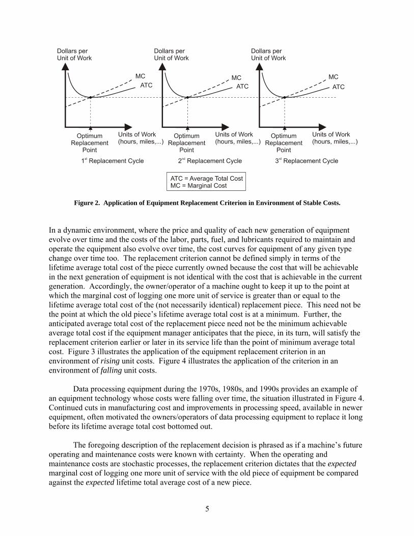
are unchanging and the costs of the labor, parts, fuel, and lubricants required to maintain and operate the equipment are also unchanging, the cost curves for every piece of a given type of equipment would retain their shape from one generation to the next. The point in a machine’s service life at which its marginal cost of operation equals the lifetime average cost of a new machine happens to be the point at which the machine’s lifetime average cost is at a minimum. At that point, the owner would sell the piece and buy an identical replacement piece, which he or she would also proceed to use up to the point of minimum average total cost. Figure 2 illustrates the application of the equipment replacement criterion in an environment of unchanging unit costs: applying the replacement criterion MCold ≤ E(ATCnew) amounts simply to minimizing the lifetime average total cost of each piece; the owner/operator of a piece would keep it until he or she had logged the number of units of service at which the average total cost reached its minimum.

5

Figure 2. Application of Equipment Replacement Criterion in Environment of Stable Costs. In a dynamic environment, where the price and quality of each new generation of equipment evolve over time and the costs of the labor, parts, fuel, and lubricants required to maintain and operate the equipment also evolve over time, the cost curves for equipment of any given type change over time too. The replacement criterion cannot be defined simply in terms of the lifetime average total cost of the piece currently owned because the cost that will be achievable in the next generation of equipment is not identical with the cost that is achievable in the current generation. Accordingly, the owner/operator of a machine ought to keep it up to the point at which the marginal cost of logging one more unit of service is greater than or equal to the lifetime average total cost of the (not necessarily identical) replacement piece. This need not be the point at which the old piece’s lifetime average total cost is at a minimum. Further, the anticipated average total cost of the replacement piece need not be the minimum achievable average total cost if the equipment manager anticipates that the piece, in its turn, will satisfy the replacement criterion earlier or later in its service life than the point of minimum average total cost. Figure 3 illustrates the application of the equipment replacement criterion in an environment of rising unit costs. Figure 4 illustrates the application of the criterion in an environment of falling unit costs.

Data processing equipment during the 1970s, 1980s, and 1990s provides an example of

an equipment technology whose costs were falling over time, the situation illustrated in Figure 4. Continued cuts in manufacturing cost and improvements in processing speed, available in newer equipment, often motivated the owners/operators of data processing equipment to replace it long before its lifetime average total cost bottomed out.

The foregoing description of the replacement decision is phrased as if a machine’s future

operating and maintenance costs were known with certainty. When the operating and maintenance costs are stochastic processes, the replacement criterion dictates that the expected marginal cost of logging one more unit of service with the old piece of equipment be compared against the expected lifetime total average cost of a new piece.

6

Figure 3. Application of Equipment Replacement Criterion in Environment of Rising Costs.

Figure 4. Application of Equipment Replacement Criterion in Environment of Falling Costs.

PURPOSE AND SCOPE

The purpose of this study was to determine whether a better, statistically based method for making replace/repair decisions could be identified. In order to apply the equipment replacement strategy described previously, an equipment manager must have a reliable estimate of the marginal cost of keeping an existing piece of equipment in service and a reliable estimate of the lifetime average total cost of a replacement piece. The practical goal therefore was to

7

obtain from the available historical data the best possible estimates of the expected marginal cost of an existing piece of equipment and of the expected average cost of a new piece.

The available data on which he or she may base the estimates are (1) figures provided by

the equipment manufacturer and (2) historical cost data. The goal of this research was to obtain from the available historical data the best possible estimate of the expected marginal cost of keeping an existing piece of equipment in service.

The study did not examine certain undeniably important issues concerning equipment

replacement. It did not model the evolution of a machine’s resale value. The required time cost prevented the research team from retrieving sale prices for more than a small number of machines. The study did not determine at what point in the VDOT budget cycle the cost estimates must be provided in order to be useful to equipment managers. This issue has been studied by VDOT, and the interested reader is referred to a report by the Management Services Division (VDOT, 2003).

METHODS

The method by which the goal was pursued involved four steps: 1. Review the literature for descriptions of equipment life cycle cost patterns. In some

cases, the descriptions were verbal descriptions of the observed cost patterns, with many nuances and special cases. In other cases, the descriptions were more abstract mathematical models whose realism was tested against actual cost data. An additional step, conceived originally as a survey of the current equipment replacement practices among state departments of transportation (DOTs) and other industries that use similar heavy equipment, was made superfluous by the findings of the literature review.

2. Retrieve a base of historical equipment cost data within VDOT. For economy’s sake,

the research team selected a database of a handful of the types of equipment VDOT uses in greatest number.

3. Employ statistical methods to identify and model mathematically the patterns of life

cycle cost in VDOT equipment. 4. Derive a replace/repair decision rule that takes best advantage of the cost patterns

and recommend the procedures to implement the rule.

Literature Review

The literature review was based chiefly on the results of a search of TRANSPORT from

1988 to the present. Literature recommended by VDOT’s equipment management personnel was also included in the review. Since one of the sources found in the literature (Fluharty, 2000)

8

was a recent survey of the practice among state DOTs, an independent survey of the current practice was not conducted.

Retrieval of VDOT Equipment Cost Data

VDOT uses a custom-designed, menu-driven software package, the Equipment Management System (EMS), to keep track of its equipment. EMS processes, manages, and maintains the data files related to the equipment inventory of the Asset Management Division (VDOT, 1992). EMS consists of several subsystems, each of which performs a function or functions in one part of the life cycle of a piece of equipment.

Users who are authorized to access the system can examine and update information on

any machine in the equipment fleet or format the information for presentation in a report. A report on a single piece of equipment may choose data from any of the hundreds of numeric and alphabetic fields in the database. Some of the fields in EMS are filled in only once, when a new piece of equipment enters VDOT’s inventory. Other fields contain a running total, e.g., cost lifetime to date, that is updated periodically as the machine undergoes more use and more maintenance and repairs. The researchers’ examination of the database suggested that some of the EMS fields are updated frequently and conscientiously and others are updated with somewhat less frequency and precision.

The system is designed to facilitate keeping inventory, tracking work orders and warranty

reimbursements, and recording disposal, all essential accounting functions. Some of the reports a system user can command, such as the “Rental Equipment Operating Statement” (Command 531), provide information that is relevant to the replace/repair decision: fuel cost, parts cost, labor cost, hours used, and hours broken, year to date and lifetime to date. Figure 5 shows a sample report page generated by EMS.

Data Available in EMS Database

To model and forecast the future cost of owning and operating a piece of equipment, a historical record of each machine’s service, maintenance, and repair is required. The research team identified a list of 61 fields in the EMS database that were believed to be of possible use in modeling and forecasting. Table A1 in the Appendix lists the 61 fields. Many of these fields contain a running total that is updated periodically as a machine undergoes more use and more maintenance and repairs or a location indicator that changes if the machine is transferred to a new district office, residency, or area headquarters. Under prevailing VDOT practice, however, the values that were in these fields at any particular time were not archived. The year-to-date totals, for instance, were preserved until the preparation of the end-of-fiscal-year reports in July and August, and then they were discarded, leaving only the year-to-date totals of the new fiscal year. Similarly, only a machine’s most current garage location would be preserved in the database. Hence it was not possible to retrieve a series of snapshots of these fields at different points in time, such as the end of each fiscal year.

9

RUN DATE: 08/09/92 COMMONWEALTH OF VIRGINIA EMR531P1-01 RUN TIME: 15:20:56 DEPARTMENT OF TRANSPORTATION PAGE: 1 EQUIPMENT DIVISION RENTAL EQUIPMENT OPERATING STATEMENT MODEL YEAR 1992 DIST: 0 CENTRAL OFFICE RES: 69 EQUIPMENT DIVISION AREA: 010 EQUIPMENT DIVISION(010) CLASS: 333 LOADERS – TRACTOR RT W/BHOE 2WD FUEL COST PARTS COST LABOR COST OVHD COST DEPREC TOTAL COST HRS USED % REVENUE GAIN/LOSS EQ ID. YTD/LTD YTD/LTD YTD/LTD YTD/LTD YTD/LTD YTD/LTD YTD/LTD UTIL YTD/LTD YTD/LTD R00080 0.00 0.00 100.00- 0.00 0.00 100.00- 0.0 .0 0.00 100.00 0.00 0.00 100.00- 0.00 0.00 100.00- 0.0 0.00 100.00 R00082 0.00 0.00 0.00 0.00 0.00 0.00 0.0 .0 0.00 0.00 0.00 0.00 0.00 0.00 0.00 0.00 0.0 0.00 0.00 R00083 0.00 0.00 0.00 0.00 0.00 0.00 0.0 .0 0.00 0.00 0.00 0.00 0.00 0.00 0.00 0.00 0.0 0.00 0.00 R00084 0.00 0.00 0.00 0.00 0.00 0.00 0.0 .0 0.00 0.00 0.00 0.00 0.00 0.00 0.00 0.00 0.0 0.00 0.00 R00086 0.00 0.00 0.00 0.00 0.00 0.00 0.0 .0 0.00 0.00 0.00 0.00 0.00 0.00 0.00 0.00 0.0 0.00 0.00 R00087 0.00 0.00 0.00 0.00 0.00 0.00 0.0 .0 0.00 0.00 0.00 0.00 0.00 0.00 0.00 0.00 0.0 0.00 0.00 R00088 0.00 0.00 0.00 0.00 0.00 0.00 0.0 .0 0.00 0.00 0.00 0.00 0.00 0.00 0.00 0.00 0.0 0.00 0.00 R00089 0.00 0.00 0.00 0.00 0.00 0.00 0.0 .0 0.00 0.00 0.00 0.00 0.00 0.00 0.00 0.00 0.0 0.00 0.00 AREA TOTALS 0.00 0.00 100.00- 0.00 0.00 100.00- 0.0 .0 0.00 100.00 0.00 0.00 100.00- 0.00 0.00 100.00- 0.0 0.00 100.00 AREA TOTAL UNITS 8 AVERAGE 0.0 RES TOTALS 0.00 0.00 100.00- 0.00 0.00 100.00- 0.0 .0 0.00 100.00 0.00 0.00 100.00- 0.00 0.00 100.00- 0.0 0.00 100.00 RES TOTAL UNITS 8 AVERAGE 0.0 DIST TOTALS 0.00 0.00 100.00- 0.00 0.00 100.00- 0.0 .0 0.00 100.00 0.00 0.00 100.00- 0.00 0.00 100.00- 0.0 0.00 100.00 DIST TOTAL UNITS 8 AVERAGE 0.0 *** END REPORT *** SELECTION CRITERIA;OPTION 1; CLASS CODE 333; DISTRICT 0; MODEL YEAR 1992

Figure 5. Sample Report Page from EMS (From VDOT, 1992, pp. 10-52).

10

At the researchers’ request, equipment section staff did preserve the values of these data at the close of Fiscal Year 2002, and they provided a copy of the data to VTRC. They did this again at the close of 2003, providing a second year’s worth of observations. If they continue to do this, over time, a more comprehensive database for future equipment research will accumulate. Data Available for Immediate Analysis

The Equipment Section did preserve copies of a report on each piece of equipment, listing a small but critical set of the EMS fields desired for analysis. Five years of data, from Fiscal Years 1997 through 2001, were available. In general, data on the following variables were recorded each year for each machine: fuel cost year to date (YTD), labor cost YTD, parts cost YTD, hours used YTD, fuel cost lifetime to date (LTD), labor cost LTD, parts cost LTD, hours used LTD, location where the machine is garaged, and the equipment code and individual ID number.

The research team restricted its attention to a few types of equipment, chosen on the basis

of two criteria. First, pieces of the equipment type must be relatively plentiful. Second, the type must be in use in all, or nearly all, of VDOT’s nine construction districts. The machines included in the sample were motor graders (equipment Codes 285 and 286), wheel loaders (Codes 336, 338, and 340), pickup trucks (Codes 824 and 828), and dump trucks (Codes 864, 866, and 896). Overall, there were 21,809 observations (records), each of one machine in 1 year.

The calendar age of each machine was not part of the available cost report. By manual

queries into the on-line EMS database, the team added to the records with equipment Codes 285, 286, and 336 an additional field that showed the year in which each machine was purchased. Time did not permit this to be done for the entire set.

The research team added manually to each record a field that indicated the fiscal year in

which the record had ended. The five Excel spreadsheets of data, one for each year, were then compiled in Excel and exported to MATLAB as tab delimited text files. MATLAB is a software application equipped to perform numerical computations such as statistical analysis.

The additional variables required for regression analysis were generated from the original

variables. One-period and two-period lags of fuel cost, labor cost, parts cost, and hours used, both YTD and LTD, were created. The location data were used to create geographic dummy variables, intended to capture the impact that terrain may have on the performance, quality, or efficiency of the equipment. Initially the garage location of each piece of equipment was assigned to one of five physiographic regions as defined by the Virginia Department of Mines, Minerals, and Energy (1993): the Coastal Plain, the Piedmont (really a union of several smaller regions), the Blue Ridge, the Valley and Ridge, and the Appalachian Plateaux. The Coastal Plain was treated as the base case; four dummies were created to represent the differences in the other four physiographic regions. As only a small number of records represented the Appalachian Plateaux, this region was later combined with the Valley and Ridge, leaving three

11

dummy variables. Table A2 in the Appendix is a chart of the dependent and independent variables that were used in each statistical regression.

Observations that lacked any of the relevant variables were deleted from the sample. The team had no reason to suspect a correlation between a blank field and the true value of the field. It was therefore assumed that flaws in reporting were independent of the characteristics of a machine and that deleting incomplete records would cause no bias in statistical estimation. Records for nine machines contained obviously misreported fields, i.e., negative entries for one or more cost variables, and these, too, were omitted. Three location Codes—“Materials,” “Maintenance contract (PPTA) Dennis Shea,” and “Unassigned”—defied the researchers’ efforts to place them geographically. These also were removed from the sample. After these deletions, the size of the sample fell to 18,562 observations (records), each of one machine in 1 year. These records represented 2,225 machines for which a full 5 years of data were available and 4,862 machines for which between 1 and 5 years of data were available.

Modeling the Patterns of Life Cycle Cost in VDOT Equipment

As stated earlier, the basic goal was to predict the value of the ratio (l + p)/f, the sum of

labor and parts expense YTD per dollar of fuel expense YTD one or more years in advance. This prediction would have to be based solely on currently known values of labor, parts, and fuel expenses and geographic location, i.e., on the information included in VDOT’S 1997 through 2001 cost reports. The forecasting equation, showing the future value of (l + p)/f as a function of currently known values of labor parts, fuel, and location, would agree as much as possible with the 5 years of data available from these cost reports. Theoretical Issues in Specifying a Forecast Model

As stated earlier, the labor, parts, and fuel expenses that are needed to keep a piece of equipment in service may be characterized as stochastic processes that progress incrementally as the equipment is used and that may also jump discontinuously when a part fails or when the piece suffers an accident. Under such a regime, the outlay on parts and labor would be expected to depend on the amount of use the machine has received, the meteorological conditions in which it has been operated, and the quality or level of past maintenance outlays. The outlay on certain equipment systems may depend on other variables: for instance, the outlay on parts and labor for the engine, transmission, and drive train of a self-propelled piece would be expected to depend on the terrain in which it had been operated; the outlay on parts and labor for the body of an on-road vehicle would be expected to depend on the intensity with which the roads it traveled were salted in the winter.

In theory, maintenance outlays could also affect the other costs of operating a piece of

equipment, e.g., its fuel economy.

The literature accepts the postulate that the lifetime average unit cost plotted versus time has a U shape. The unit cost of owning a machine obviously falls steeply during its early years

12

of service. The unit cost of operating a machine rises as its moving parts undergo more use and more wear. Preliminary Statistical Analysis of the Data

The available dataset included only one direct measure of the usage of a piece of equipment: hours of use. Discussions with equipment section staff cast some doubt on the completeness and reliability of the data in this field. This doubt persuaded the research team to choose fuel expense, rather than hours of use, as the most plausible measure of machine usage. This choice precluded the computation of average fuel economy over the course of a year and consequently precluded estimation of the relationship between fuel economy and maintenance expenses.

In addition to giving up the opportunity to regress fuel expense against hours of use, the

choice of fuel expense as the measure of use introduces another problem. Fuel consumption, and therefore fuel expense, obviously depends directly on usage, but fuel expense also depends directly on the price of fuel. As a measure of use, fuel expense would be better deflated by a fuel price index. On the other hand, because the labor and parts expenses are also subject to general price inflation, the inflation component in the sum of labor and parts expenses will tend to negate the inflation component in fuel expense when their ratio is computed. All of the findings reported here result from statistical analyses in which neither fuel expense nor labor and parts expenses were adjusted for inflation.

For equipment Classes 285 (150-hp motor grader), 336 (110-hp wheel loader

w/backhoe), and 338 (110-hp wheel loader), the correlation coefficients among the available variables were computed. This preliminary analysis showed no obvious correlation between the geographic location dummies and the other variables, with the coefficients mostly less than 0.3. It did show that parts cost LTD, labor cost LTD, fuel cost LTD, and calendar age were strongly correlated, with coefficients mostly above 0.6 and often greater than 0.7. This meant that it would be difficult to separate the influence of these variables statistically unless a good deal of structure was imposed a priori on the regression equation.

As another preliminary test, the research team sorted the observations into artificial

discrete “cells,” based on the fuel expense LTD and the sum of labor and parts expenses YTD: each bin represented a specified range of fuel expense LTD and a specified range of labor and parts expense YTD. For each class of equipment separately, the number of observations in each cell was counted and the tallies were displayed in a histogram. For any given range of fuel expense LTD, the histogram of labor and parts expenses YTD revealed a lopsided bell curve, unimodal and skewed right; i.e., even cells representing very high values of labor and parts expense were often not empty. When the mean, mode, and variance of the distribution of labor and parts expense were computed for each range of fuel expense, they were found to increase as fuel expense increased; i.e., the higher the fuel expense LTD, the more the bell curve stretched and the further its peak moved to the right. In plain terms, this finding means that among the pieces of equipment of any given age, a few rang up costs much higher than the average for their group. Further experimentation along the same lines established that if the data were sorted into

13

cells based on the fuel expenses LTD and on the quantity (labor + parts YTD) ÷ (fuel LTD)0.6, the distribution of that quantity (labor + parts YTD) ÷ (fuel LTD)0.6 was also unimodal and skewed right for any given range of fuel expense LTD. However, the mean, mode, and variance of the distribution (i.e., the shape of the bell curve) remained approximately constant as fuel expense LTD increased. From this finding, it could be inferred that that the variance of the labor and parts expense YTD over a population of equipment varies approximately in proportion as the fuel expense LTD varies. Consequences for the Cost Specification

The objective was a cost forecasting equation that was not too complicated and that fit the available cost data reasonably well. It must be kept in mind that an upward-sloping average variable cost curve (i.e., a steadily rising average unit operating cost) is part of the cause of a U-shaped average total cost curve (i.e., a life cycle cost that first falls and then rises). The researchers’ a priori understanding of the shape of the cost curves and the preliminary statistical tests led them to experiment with models that would have right-skewed error terms and to look for parameter values that comported with the U-shaped cost curve. The specification began with simple cost models in which the operating cost was the sum of labor and parts expenses, L + P, and was a function of fuel expense F.

Consider the cost specification

( )tttt FPL iiiε

βα β

⋅⋅+

=++ )(

1)()( 1 (1)

where Li(t), Pi(t), and Fi(t) are LTD expenses on labor, parts, and fuel; α and β are parametric constants; and ε is an error term. The postulate that the average operating cost rises as fuel consumption rises amounts to the assumption that the parameter β is positive. One possible error distribution that would be skewed right would be the case in which the change in the error term from one time t1 to another time t2 was a lognormal variable with variance proportional to the square root of |t1 – t2|.

Consider the alternative cost specification

( ) ( )tetbab

tt FPL iii⋅⋅+⋅=+ )(exp1)()( (2)

where a and b are constants and e is an error term. The postulate that the average operating cost rises as fuel consumption rises amounts to the assumption that the parameter b is positive. As in the previous case, an error term whose first difference over an interval of time was a lognormal variable is one of a number of possibilities that would produce a right-skewed distribution. Including Influence of Geography

Geography may be expected to have an impact at least on the operating cost of self-propelled equipment. Greater topographical relief, with its correspondingly steeper grades,

14

ought to be positively correlated with cost. Likewise, the frequency of freezing temperatures, occasioning more cold starts, ought to be positively correlated with cost. It should be noted that steep grades and low temperatures may also be positively correlated with fuel consumption per hour or mile service, so using fuel cost as the measure of use may prevent detection of these relationships even if they are present.

Given the way that the geographic dummy variables were constructed to represent

Virginia’s physiographic regions, one would expect each of the dummies to have a positive regression coefficient when they are included in the regression. The Appalachian Plateaux/Valley and Ridge dummy ought to have the largest positive coefficient, and the Piedmont dummy the smallest. On these grounds, then, a statistical regression that estimated positive values for the coefficients of the location dummy variables would tend to corroborate the reasonableness of a given model whereas a regression that produced negative coefficient values would tend to cast doubt on the model. Implications for Forecasting: The Logarithmic Specification

Algebraic development of Equation 1 shows that under this simple specification (geographic dummies are not included), the expected unit cost of machine i during the coming year t + 1 is approximately proportional to the lifetime fuel expense raised to the power β, the factor of proportionality being α:

( ) ( ).

)1()1()1(

tt

ttE FF

PLi

i

ii βα ⋅≈⎥⎦

⎤⎢⎣

⎡

+∆+++∆

(3a)

This implies, alternatively, that the expected unit cost in year t + 1 is approximately

proportional to the lifetime average unit cost as of the previous year t:

( ) ( ))(

)()(1

)1()1()1(

ttt

ttt

EF

PLF

PLi

ii

i

ii+

⋅+≈⎥⎦

⎤⎢⎣

⎡

+∆+++∆

β . (3b)

Regression analysis was used to estimate the equations in their logarithmic forms.

( ) ( )tt

ttFF

PLi

i

ii lnln)1(

)1()1(ln ⋅+≈⎥

⎦

⎤⎢⎣

⎡

+∆+++∆

βα (4a)

( ) ( ) ⎟⎟⎠

⎞⎜⎜⎝

⎛ +++≈⎥

⎦

⎤⎢⎣

⎡

+∆+++∆

)()()(

ln1ln)1(

)1()1(ln

ttt

ttt

FPL

FPL

i

ii

i

ii β (4b)

Thus, regression analysis based on the specification in Equation 1 was used to obtain

estimates of the parameters α and β in that equation.

15

It can also be shown that, ignoring the salvage value and ignoring price changes, the minimum achievable average total cost of a machine that conformed to this model would be

⎟⎟⎠

⎞⎜⎜⎝

⎛+⋅ +

+ ⋅=1

11

1min β

βα β

ββ

PPATC (5)

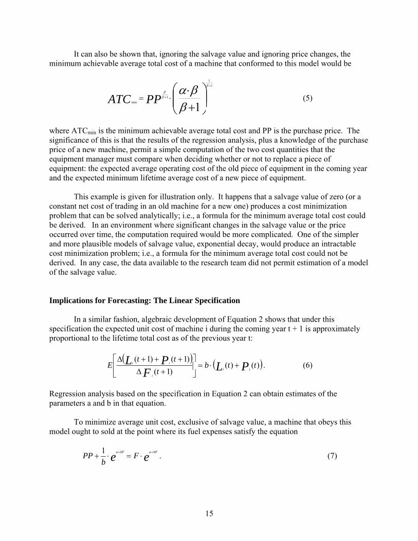
where ATCmin is the minimum achievable average total cost and PP is the purchase price. The significance of this is that the results of the regression analysis, plus a knowledge of the purchase price of a new machine, permit a simple computation of the two cost quantities that the equipment manager must compare when deciding whether or not to replace a piece of equipment: the expected average operating cost of the old piece of equipment in the coming year and the expected minimum lifetime average cost of a new piece of equipment.

This example is given for illustration only. It happens that a salvage value of zero (or a

constant net cost of trading in an old machine for a new one) produces a cost minimization problem that can be solved analytically; i.e., a formula for the minimum average total cost could be derived. In an environment where significant changes in the salvage value or the price occurred over time, the computation required would be more complicated. One of the simpler and more plausible models of salvage value, exponential decay, would produce an intractable cost minimization problem; i.e., a formula for the minimum average total cost could not be derived. In any case, the data available to the research team did not permit estimation of a model of the salvage value.

Implications for Forecasting: The Linear Specification

In a similar fashion, algebraic development of Equation 2 shows that under this specification the expected unit cost of machine i during the coming year t + 1 is approximately proportional to the lifetime total cost as of the previous year t:

( ) ( ))()(

)1()1()1(

ttbt

ttE PLF

PLii

i

ii +⋅=⎥⎦

⎤⎢⎣

⎡

+∆+++∆

. (6)

Regression analysis based on the specification in Equation 2 can obtain estimates of the parameters a and b in that equation.

To minimize average unit cost, exclusive of salvage value, a machine that obeys this

model ought to sold at the point where its fuel expenses satisfy the equation

ee bFabFa Fb

PP ++⋅=⋅+

1 . (7)

16

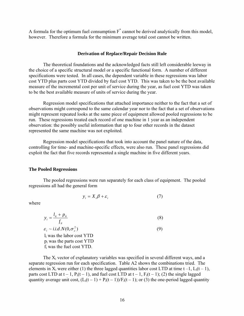
A formula for the optimum fuel consumption F* cannot be derived analytically from this model, however. Therefore a formula for the minimum average total cost cannot be written.

Derivation of Replace/Repair Decision Rule

The theoretical foundations and the acknowledged facts still left considerable leeway in

the choice of a specific structural model or a specific functional form. A number of different specifications were tested. In all cases, the dependent variable in these regressions was labor cost YTD plus parts cost YTD divided by fuel cost YTD. This was taken to be the best available measure of the incremental cost per unit of service during the year, as fuel cost YTD was taken to be the best available measure of units of service during the year.

Regression model specifications that attached importance neither to the fact that a set of

observations might correspond to the same calendar year nor to the fact that a set of observations might represent repeated looks at the same piece of equipment allowed pooled regressions to be run. These regressions treated each record of one machine in 1 year as an independent observation: the possibly useful information that up to four other records in the dataset represented the same machine was not exploited.

Regression model specifications that took into account the panel nature of the data,

controlling for time- and machine-specific effects, were also run. These panel regressions did exploit the fact that five records represented a single machine in five different years. The Pooled Regressions

The pooled regressions were run separately for each class of equipment. The pooled regressions all had the general form

iii Xy εβ += (7) where

it

ititi f

ply

+= (8)

),0(...~ 2εσε Ndiii (9)

li was the labor cost YTD pi was the parts cost YTD fi was the fuel cost YTD. The Xi vector of explanatory variables was specified in several different ways, and a

separate regression run for each specification. Table A2 shows the combinations tried. The elements in Xi were either (1) the three lagged quantities labor cost LTD at time t –1, Li(t – 1), parts cost LTD at t – 1, Pi(t – 1), and fuel cost LTD at t – 1, Fi(t – 1); (2) the single lagged quantity average unit cost, (Li(t – 1) + Pi(t – 1))/Fi(t – 1); or (3) the one-period lagged quantity

17

(li(t – 1) + pi(t – 1))/fi(t – 1) and the two-period lagged quantity (Li(t – 2) + Pi(t – 2))/Fi(t – 2). Because the theory and the basic facts did not rule out either a linear or a logarithmic relationship, equations containing the simple values of these quantities and equations containing the logarithms of their values were both tried. In some regressions, the calendar age of the machine, ai, was also an element of Xi. Every specification included a vector of geographic dummy variables, Ri, with the Coastal Plains region being the baseline. The Linear Regressions

The linear regressions, using yi as the dependent variable, could represent a model with a

U-shaped average cost curve. A look back at Equation 6 shows that the linear regression equation, with the right parameter values (namely, positive and equal coefficients on L and P), could represent the linear model developed from Equation 2. However, under every specification of the independent variables Xi, the regressions run using ln(yi) as the dependent variable explained more of the variance, and produced more precise parameter estimates, than those run using yi. Therefore the results of the regressions using yi are not presented.

The Log Regressions Using LTD Average Unit Cost

Tables A3 and A4 in the Appendix show the results of the regressions

iit

ititi PDBRVR

FPL

y εβββββ +++++

+=−

−−5432

1

111)ln( (10a)

i

it

ititi PDBRVR

FPL

y εβββββ ++++⎟⎟⎠

⎞⎜⎜⎝

⎛ ++=

−

−−

5432

1

111 ln)ln( (10b)

The geographic dummies represent the Piedmont (PD), Blue Ridge (BR), and Valley and

Ridge/Appalachian Plateaux (VR) regions. Comparison with Equation 4b reveals that with the right parameter values (i.e., β1 > 1, β2 = 1), the regression Equation 10b could represent the logarithmic model developed from Equation 1. The Log Regressions Using LTD Labor, Parts, and Fuel Expenses Individually

Tables A5 and A6 in the Appendix show the results of the regressions

iitititi PDBRVRFPLy εβββββββ +++++++= −−− 7654131211)ln( (11a)

( ) ( ) ( ) iitititi PDBRVRFPLy εβββββββ +++++++= −−− 7654131211 lnlnln)ln( (11b)

Comparison with Equation 4a reveals that with the right parameter values (i.e., β2 = β3 = 0, β4 > 0), the regression Equation 11b could represent the logarithmic model developed from Equation 1.

18

Panel Regressions

These specifications allow time series effects to enter only through the presence of lag terms, with the regression treating every observation as if it pertained to a different piece of equipment and the year of the observation being irrelevant. This approach makes some non-trivial assumptions. The key assumption is that each machine’s unit cost from one year to the next is uncorrelated with its cost in previous or future years, except insofar as this correlation is captured by last year’s cumulative average. It is possible, however, that there are machine-specific and/or time-specific components of the unit cost that the analyst cannot observe.

Estimating a model that allows for these unobserved machine-specific or time-specific

components requires a slightly more sophisticated technique. The machine-specific effect can be taken into account in one of two ways: it may be treated as a random effect or it may be treated as a fixed effect.

The first approach was rejected. The random effect treatment produces meaningful

results only if the random machine-specific effect can be assumed to be uncorrelated with the other explanatory variables, and such an assumption seemed questionable in the case at hand. Any measure of the machine’s cost or use LTD would almost surely be correlated with the machine-specific component of average cost YTD, and the coefficient estimates would be biased and inconsistent.

The second approach was adopted. The fixed effect treatment involves the introduction

of a unique dummy variable for each machine in the sample, save one. This two-step approach to estimation will yield consistent estimates of the parameters associated with time-varying variables. Generally, the information about the parameters associated with time-invariant variables (i.e., the geographic dummies) will be lost because the regression procedure differences out the mean over time and the machine-specific effect and the geographic effect will not be separately identifiable (see Hsiao, 1986).

These models took the general form

itiiitit RXy εαµγβ ++++= (12)

where the vector Xi represented the same range of options as in the pooled regressions, Ri represented the vector of time-invariant variables (the geographic dummies), µ represented the overall mean machine-specific effect, αi represented the fixed effect of machine i measured as a deviation from the mean µ, and εit was a random unobservable (i.e., an error term). Estimation of Equation 12 was the first step of a two-step process. The “within estimator” that emerged from this procedure yielded a consistent estimate of the parameter vector β.

This estimator was then used to construct the regression equation

( )iiiii RXy εαµγβ +++=− ˆ (13)

19

A consistent estimate of the parameter vector γ was obtained by treating αi + εit as the error term and running an ordinary least squares regression. Tables A7 and A8 in the Appendix show the results of the two-step regressions using the LTD average unit cost, Y = (L + P)/F, and the geographic dummies as the explanatory variables. Tables A9 and A10 show the results of the two-step regressions using the LTD labor, parts, and fuel expenses, L, P, and F, and the geographic dummies.

Given the shallowness of the panel in the time dimension, i.e., only 5 years of

observations being available, it was unclear that the consistency of the estimator of γ (i.e., its tendency to converge on the true value of γ as the size of the sample increases) would guarantee an estimate centered on the true value. Evidence or theoretical grounds on which to assert that Ri and αi must be orthogonal (uncorrelated) was lacking. If the observable variables Ri were correlated with the unobservable machine-specific parameter αi, then the estimates of µ and γ would not be consistent, though the estimate of β would remain so.

RESULTS AND DISCUSSION

Literature Review

The replace/repair decision, as with the other parts of the operating strategy, has as its goal maximizing the return on the equipment dollar. Any agency or business that operates a fleet of machines faces this challenge. For this reason, experts from several industries, including construction, freight transport, and public transit, have made contributions to the literature concerning equipment replacement. Scope of Equipment Management Literature

Experts in the public and private sectors have been writing about equipment management for more than 80 years. The oldest document the research team examined, Dudick and Ravenscroft (1966), cited the fifth edition of Contractors’ Equipment Ownership Expense but made mention of the first edition, which was published in 1920. Fluharty (2000) cited a 1987 article by Vorster and Sears, who also surveyed the literature back to the 1920s.

Morris (1978) surveyed the state of the practice as of 1978. A national pooled-fund

study, launched in 1975 under the auspices of the Federal Highway Administration (FHWA), produced an equipment management system manual in June 1978 (Cresap, McCormick and Paget, Inc., 1978). Reflecting a concern with the lack of political and administrative support for timely equipment replacement, both publications discussed how information may be used “better [to] communicate the need for equipment replacement to support highway maintenance and betterment programs and [to] demonstrate the cost consequences of not meeting these needs” (Cresap, McCormick and Paget, Inc., p. II-12).

20

Fluharty (2000) surveyed practices as of 1998 and compared the findings with those of Morris (1978). The author found that although many more agencies were collecting and banking data in 1998 than in 1978, they did not rely more heavily on data analysis in 1998 than in 1978.

The Transportation Research Board’s (TRB) Committee on Maintenance Equipment

(2002) described the customary rental, lease, and purchase options available to equipment fleet managers. They explained how to compare different bids and lists factors, such as duration of need and degree of control over cash flow, that should be taken into account. The current research addresses the narrow questions of forecasting future maintenance and operation costs and of forecasting the resale value of a piece of equipment. It explains clearly that these forecasts alone do not dictate the choice between replacement and repair of an aging machine. A variety of additional factors, among them the price of new equipment, the continuing need for machines of that type, and the budget at the manager’s disposal, will also enter into the choice.

A number of college textbooks cover the basics of equipment management. These books

include a discussion of the economic aspects of equipment management: the computation of ownership and operating costs, the strategies of fleet management, and so forth (see Nunnally, 2000; Schaufelberger, 1999). As automobile and truck fleets are far more numerous than are those of other types, entire books devoted to their management exist (see Dolce, 1984).

Hanson and Kyte (1999) reported regression estimates of linear forecasting models of the

resale price and the unit operating cost of four types of state pool passenger vehicles. Weissmann et al. (2003) used a model of the time path of life cycle cost to derive a statistic that is meant to identify, within any given equipment class, those pieces that are likely to have the highest cost per unit of service during the ensuing year. Classification and Reporting of Equipment Costs

The classification of the costs of owning and operating a machine appears to have been settled by the 1960s. A component of cost attributed to a particular machine may be direct, i.e., traceable to the ownership or operation of that machine, or indirect, i.e., traceable no further than to the ownership and operation of the entire fleet, or to the suite of machines on a particular project. A component of cost may be fixed for a time, for instance 1 year, or it may vary daily depending on the use to which the machine is put. The identification of a cost component as either a cost of ownership or a cost of operation usually matches closely the division between fixed and variable costs. Although the treatment of costs differs in minor details from one text to another, the classification shown in Figure 6 is typical. The figure shows that with the exception of depreciation, the costs of equipment ownership are all fixed costs; the costs of operation are all variable costs, although the action that triggers some of these costs is the deployment to a work site rather than the hour or mile of service on the site.

The range of acceptable ways of recording and allocating equipment costs for purposes of

computing tax liability or making cost comparisons continues to evolve, but the range is well defined and fairly narrowly restricted. The challenge for the equipment manager is forward

planning. Many of the cost components depend, in part, on events that cannot be predicted in

21

Figure 6. Classification of Equipment Costs. advance. Depreciation due to obsolescence, for example, depends on the introduction of improvements to new equipment. Repair costs depend on the number and nature of accidents and breakdowns.

All sources agree that complete records are critical. It is not possible to monitor the cost

of a machine, nor therefore to make an informed decision to repair it or sell it, without consulting the history of its usage, its fuel consumption, its maintenance and repair expenses, its downtime, and the intervals between parts replacement.

22

Prospective Modeling of Equipment Costs

As stated earlier, historical data (see Cresap, McCormick & Paget, Inc., 1978; see Weissmann et al., 2003) showed that the life cycle cost of an owned piece of equipment, charted as a function of time, tends to have a U shape: the cost per unit of service declines during the early years of operation, bottoms out, and then begins to rise.

In contrast to the classification and reporting of cost elements, the modeling and

forecasting of cost have evolved rapidly in the past few decades. Dudick and Ravenscroft (1966) presented a rental rate formula that took account of both operating costs and ownership costs. The focus was on rental rates for a class of equipment rather than on diagnostic analysis of individual pieces. The only forward-looking cost element in their model was depreciation, which depended on an estimate of the machine’s expected service life. The other cost components, including all operating costs, were simply historical averages.

Cresap, McCormick and Paget, Inc. (1978) included the graphical exposition of average

fixed and variable costs that is the model for Figures 1 through 4. The model was also formalized in a table rather than an equation. This exposition modeled the expectation that the cost of maintaining and operating a machine will rise as the machine is used and demonstrated the result: a number of hours of service at which average cost is a minimum. The manual concluded:

Based on the foregoing analysis, to support equipment planning and to permit users and field supervisors to identify specific units for replacement, the equipment manager should establish replacement standards for equipment in all classes. The standards should be established by equipment class and should identify a target level of usage that units should accumulate. . . . However, the decision to replace a given unit should be based on an analysis of the utilization and cost history of that unit (p. II-24).

Cresap, McCormick and Paget, Inc., explicitly discussed overhaul as a third option, in addition to the choices of using a piece of old equipment as-is or of replacing it with a new piece.

Hanson and Kyte (1999) studied the replacement criterion for the passenger vehicles

under the control of VDOT’s Division of Fleet Management. They modeled a vehicle’s sales price at auction as a linear function of its purchase price and its age, with the parameters allowed to vary according to the vehicle type (e.g., compact, mid-size, van). They modeled a vehicle’s operating cost per mile as a linear function of its age, with the age parameter and the constant allowed to vary according to type. They also computed the average annual mileage for vehicles of each type. The regression equations, combined with the average annual mileage statistics, permitted a computation of the mileage point at which a vehicle of any given type should be surplused in order to minimize the life cycle cost of operating vehicles of that type.

Weissmann et al. (2003) created and applied in the Texas DOT an automated method of

ranking the pieces of equipment of any one type in the fleet. The method used historical cost data to compute a set of statistics for each machine and to compare those statistics against the statistics of the other pieces in the fleet. The statistics included the equivalent uniform annual cost (EUAC), the cumulative usage, and a “trend score” whose sign and magnitude are intended

23

to indicate whether the machine’s average cost per hour of service has begun to rise and how fast it is rising. The definition of EUAC is identical with the definition of life cycle cost in the theoretical discussion presented earlier. The authors described the motivation for their model as follows: “The most relevant information provided by a life cycle cost graph is its trend. Units whose life cycle costs have been increasing longer and/or at a faster rate should have higher replacement priority” (p. 1). They deemed the chief challenges to a computerized equipment replacement methodology to be (1) the quality of the historical cost data and (2) the inevitable random fluctuations in the life cycle cost of any individual piece of equipment.

To address the first challenge, Weissmann et al. (2003) conducted extensive tests of the

internal consistency and completeness of the data in the TxDOT equipment database to assess the quality of the historical data. They found the quality of the data, by these two standards, to be quite good. To address the second challenge, the authors designed a statistic: the trend score. The trend score sums the annual percentage changes in a machine’s life cycle cost. It was hoped that in this sum the “white noise” in the year-to-year fluctuations in the machine’s cost record would average out and the underlying downward or upward trend would be captured. A machine whose expected average cost curve is climbing steeply with increasing usage will tend to have a higher trend score than one whose average cost is flat or climbing very gradually. A machine that has been in service long past the point of minimum average cost will tend to have a higher trend score than one that has only recently passed that point.

The basic point is that a positive trend score statistic indicates that a machine has been in

service past the point of minimum average cost and thus that a new machine can do the same job more cheaply. The bigger the machine’s trend score, the greater the costs that the equipment manager can avoid by replacing it promptly. With reference to Figure 2, the piece should be sold when its hours or miles of service bring it up, or past, the minimum point the U-shaped life cycle cost curve.

Weissmann et al. (2003) proposed that the trend score be consulted in combination with

other “attributes,” such as the machine’s actual average cost. They had good reason for doing so. For one thing, the trend score is a unitless measure of how fast a piece’s average cost is rising. The actual average cost must be consulted to determine whether a given piece costs more to operate than do others of its type. For another thing, the theoretical exposition showed that, in general, the optimal disposal point coincides with the point of minimum life cycle cost only if the manager is operating in an economic environment where the factors that tend to depress the acquisition cost of new equipment, such as productivity-enhancing design improvements, more or less offset the factors that tend to raise the acquisition cost, such as inflation. If the expected average cost of owning and operating a new machine has risen over time; e.g., Figure 3 shows that the cost-minimizing strategy is to continue to operate an old machine beyond the point where the life cycle cost bottomed out.

To look at the same fact from a different angle, the life cycle cost (what Weissmann et al.

called the equivalent uniform average cost) includes the acquisition cost of the old piece of equipment. In economists’ terms, the acquisition cost is a “sunk cost,” irrelevant to the equipment manager’s decision. Only the expected future operating cost of the old machine, and

24

future changes in its salvage value, needs to be weighed against the acquisition cost and expected operating cost of the new machine. Survey of Current Practice VDOT

EMS produces reports that enable the equipment managers to “flag” pieces of equipment whose accumulated lifetime cost, calendar age, or hours of use exceed specified threshold values (see VDOT, 1992). The salient features of EMS are described in more detail later. Use of cumulative usage as a flag to target pieces of equipment for possible replacement is consistent with the recommendation in the FHWA manual (Cresap, McCormick and Paget, Inc., 1978). Other Agencies

Fluharty (2000) surveyed practices in effect in May and June 1998. As noted earlier, the author compared his findings with those of Morris (1978). He concluded, perhaps with some surprise: “Twenty years later, many more transportation agencies collect data. However, these agencies tend to rely on equipment users’ judgments rather than data analysis. Almost three-fourths of the 1998 respondents reported determining equipment needs largely by roundtable discussion with district managers” (Fluharty, p. 12). A key to explaining the finding lay in the measure of “success” that the equipment managers themselves used: success was to obtain from the authority that oversees the equipment budget both permission and money to buy new equipment. “Based on informal discussion with equipment managers, this increase is attributed to the recent emphasis on ‘customer’ orientation. The customer emphasis also exists in replacement requests. From these discussions, equipment managers can better articulate replacement needs. This has resulted in transportation agencies, in general, being more successful replacing equipment in 1998 than in 1978” (Fluharty, p. 12).

In other words, the equipment managers at many agencies found the anecdotal results of

a roundtable discussion to be more persuasive than data analysis.

The low use of life cycle costing [one fourth of responding agencies] is likely due to its inconsistent impact on replacement decision effectiveness. Data analysis reveals that transportation agencies that never apply the tool are more successful in equipment replacement than those who regularly apply it. Those who rarely apply it are nearly as successful as those who frequently do so (Fluharty, p. 13).

Weissmann and Weissmann (2002) reported that the TxDOT Equipment Replacement

Model (TERM) was using threshold values for equipment age and cumulative usage of an equipment unit as inputs for replacement. For example, current threshold values for dump trucks with tandem rear axles (Class Code 540020) for age and usage were 10 years and 150,000 miles, respectively. They observed that units whose total repair costs exceed a particular “exception threshold,” a percentage of the original purchase cost, were also targeted. As noted earlier, Weissmann et al. (2003) have undertaken to revise the practice in Texas.

25

Summary of Literature Findings

The equipment management literature agrees on some basic patterns of equipment unit cost. There is a component (the acquisition cost per unit of service) that declines inexorably, at a declining rate, as the equipment is used. There is a component (the unit operating cost) that tends to rise as the equipment is used, at least after the first years of service. That component, however, is subject to random influences that can cause it to fluctuate up or down by a particular amount in any given year. Any attempt to forecast the operating cost must employ statistical techniques to mute the “noise” of these random influences.

A recent survey of the practice in the United States (Fluharty, 2000) found that the

equipment managers in many state DOTs rely primarily on the first-hand testimony of field staff who operate the equipment and only secondarily on the cost data that are collected. The survey found further that this approach appears to be effective, at least as effective as a quantitative approach, in procuring money and permission to purchase new equipment.

However, attempts to improve the quantitative approach to the identification of

equipment ripe for replacement are afoot. Hanson and Kyte (1999) and Weissmann et al. (2002, 2003) illustrate two such attempts.

Model Selection

As described in the Methods section, the research team constructed for each record in the database the dependent variable (l + p)/f, the average labor and parts expense per dollar of fuel expense YTD. They regressed this variable on a list of predictors that either included (L + P)/F, the average labor and parts expense per dollar of fuel expense LTD or included separately the LTD quantities L, P, and F. Sometimes a set of geographic region indicators and/or a calendar age variable was also included. Because the literature and the basic facts of equipment costs did not imply that the YTD unit cost must have a linear relationship with the predictors, the research team also employed the logarithmic form ln((l + p)/f) as a dependent variable.

The findings may be summarized by the statement that the “log-log” model specification, in which the natural logarithm of the YTD average unit cost was treated as a linear function of the natural logarithm of the previous year’s LTD average unit cost, or as a function of the previous year’s LTD labor, parts, and fuel expenses individually, provided the best fit to the data for most of the equipment types studied. The “log-linear” model specification, in which the natural logarithm of the year-to-date average unit cost was treated as a linear function of the previous year’s life-to-date average unit cost, or as a function of the previous year’s life-to-date labor, parts and fuel expenses individually, sometimes provided a decent fit to the cost data, but sometimes contradicted a priori expectations. The “linear-linear” model specification provided the worst fit to all sets of cost data except those for the pick-up trucks. None of the models fit the pick-up trucks’ cost data at all well.

The results of the pooled regressions using the first specification (Equation 10) are listed

in Tables A3 and A4 in the Appendix. Table A3 shows the regressions results using a log-linear

26

specification, where the independent variables Xi are the simple values of the explanatory variables L, P, and F (i.e., labor, parts, and fuel expenses LTD). Table A4 shows the results using a log-log specification, where the independent variables Xi are the natural logarithms of the explanatory variables. The relevant coefficient estimates are listed on the table with their t-statistics reported directly below the estimates. The results of the pooled regressions using the second specification (Equation 11) are listed in Tables A5 and A6, following the same format. Table 5 shows the regressions results obtained using the log-linear specification. Table A6 shows the results obtained using the log-log specification.

The picture of the relationship between the unit cost and the explanatory variables was

sufficiently fuzzy that only its most basic features could be described. The margin of error in all of the regression equations was substantial. Rarely was the estimate of any parameter, other than the constant, found to differ significantly from zero: in other words, the predictive power of the explanatory variables could not be proven conclusively (exceptions appear in Tables A3 and A4). This general inconclusiveness is believed to reflect the limitations of the available data set because an ideal model specification would take account of downtime (e.g., the “hours broken” fields in EMS) and mileage (the “miles” fields in EMS), data that were unavailable for this study. Nonetheless, some patterns can be seen in the results.

Comparison of Table A5 and Table A6 in the Appendix, or of Table A3 and Table A4,

shows that the log-log specification generally provided a better fit (a higher R2) than the log-linear specification. In other words, the log-log equation explained more of the variation in the dependent variable.

Tables A5 and A6 show the regression results using lifetime labor, parts, and fuel costs

(L, P, and F) as separate predictors of the coming year’s average labor and parts expenses. Tables A3 and A4 show the results using the ratio (L + P)/F as the predictor. Comparison of Table A3 and Table A5, or of Table A4 and Table A6, shows that the specifications that used L, P, and F separately appeared to provide a slightly better fit for motor graders (equipment Codes 285 and 286) and wheel loaders (Codes 336, 338, and 340), and a considerably better fit for pick-up trucks (Codes 824 and 828) and dump trucks (Codes 864, 866, and 896).

Although the R2 statistics appeared to favor the specifications that used L, P, and F as

separate regressors, the estimated values of the coefficients provided ambiguous support for the specifications that used the ratio (L + P)/F. Table A4 indicates that in the log-log regressions the constant term β1 was estimated to be greater than zero, with statistical significance except in the case of equipment Class 340 (140-horsepower, 3-cubic-yard wheel loaders). With reference to Equation 4b and the theoretical basis of the regression equations, this implied that the curvature parameter β in Equation 1 was positive. This is consistent with a life cycle cost curve (a.k.a. an average total cost curve) that has a U shape, as postulated. Table A5, on the other hand, indicates that in the log-linear regressions, the coefficient β4 was estimated to be greater than zero in only 3 of 10 equipment classes, two of the three being the pickup trucks (Class Codes 824 and 828). Only a positive value was consistent with a U-shaped average cost curve, but the presence of labor and parts expenses, both of which were highly correlated with fuel expense, among the explanatory variables could explain why this regression failed to produce the expected results.

27

For some of the equipment types, regressions of Equations 10 and 11 were run with the independent variable calendar age included as an extra variable. The results of these are not reported. The estimated value of the coefficient on age was sometimes positive, sometimes negative, and relatively small (generally much smaller, for instance, than the coefficients on the geographic dummies). This suggested that once the number of units of service and the geographic location are taken into account, the chronological age of a machine contributes little to a forecast of the machine’s future unit costs.

The results of the panel regressions using Equations 12 and 13 are listed in Tables A7

through A10 in the Appendix. The estimates of the coefficients on the geographic dummies often had different signs in the panel regression results than they did in the pooled regression results of Table A3 in the Appendix. This suggested that the pooled regression technique produced seriously biased estimates of the influence of geography, but as the coefficients were too close to zero to be statistically distinct, it was not possible to draw a firm conclusion.

The fitted log-log cost model was consistent with the supposition that the life cycle cost

curve (a.k.a. the lifetime average total cost curve) is U shaped. In other words, the estimate of the critical parameter supported the conventional wisdom that the average variable cost climbs as a machine is used more and more and that as the average fixed cost (acquisition cost per unit of service) approaches zero, the average total cost will eventually begin to rise. The amount by which the incremental cost per unit of service (a.k.a. the marginal cost) exceeded the historical average unit cost appeared to vary from a factor of 2 (i.e., +100%) for certain equipment types, such as the 150-horsepower motor grader, to a factor of 1.3 (i.e., +30%) for other types, such as the 110-horsepower, 2-cubic-yard wheel loader with backhoe.

The critical parameter in the log-linear model, on the other hand, did not always have the

expected positive sign. The fitted log-linear model therefore was not always consistent with the U-shaped cost curve.

Under the reasonably well-fitting cost model (shown in Equations 1, 4b, and 10b), the

average unit cost YTD is equal to a constant (β + 1) times the previous year’s average unit cost LTD. The ratio of these two quantities is therefore an estimate of that constant:

( )

( ) 1111

+=+

∆+∆

−−−

βFPLFPL

ttt

ttt (14)

This implies in turn that the ratio can be multiplied by the current year’s average unit cost

LTD to forecast the average unit cost YTD for the coming year or, by repetition, for any future year.

The historical average unit cost (represented in this report by labor cost LTD plus parts cost LTD as percentages of fuel cost LTD) provides a measure of a machine’s performance to date. The first conclusion implies that, except in the event of extraordinary repairs, this average should be expected to rise over time. The ratio between the previous year’s unit cost (represented by labor cost YTD plus parts cost YTD as percentages of fuel cost YTD) and the

28

lifetime average unit cost provides a measure of how fast the machine’s average cost should be expected to rise.

Replace/Repair Decision Rule and Procedures to Implement it

Equipment managers should compute for each piece of equipment the ratio between the most recent year’s average unit cost YTD and the previous year’s average unit cost LTD (see Equation 14). This will permit an estimate of the machine’s future unit cost. To be specific, the formula

( )( )

( )⎥⎦

⎤⎢⎣

⎡

∆+∆

=+

×+

∆+∆

+

++

−−− FPL

FPL

FPLFPL

t

tt

t

tt

ttt

ttt Expected1

11

111

(15)

is a forecast at the end of year t of a machine’s unit cost in the year t + 1. This forecast is likely to be rather volatile, and therefore rather unreliable, for a piece of equipment that has been in use for less than 3 years. The ratio on the left may be replaced by an average taken over 2 or more years or by the estimated coefficient β1 from the regression Equation 10b.

CONCLUSIONS • The “log-log” model specification, in which the natural logarithm of the YTD average unit

cost was treated as a linear function of the natural logarithm of the previous year’s LTD average unit cost, or as a function of the previous year’s LTD labor, parts, and fuel expenses individually, provided the best fit to the data for most of the equipment types studied.

• The “log-linear” model specification, in which the natural logarithm of the YTD average unit

cost was treated as a linear function of the previous year’s LTD average unit cost, or as a function of the previous year’s LTD labor, part, and fuel expenses individually, sometimes provided a decent fit to the cost data, but sometimes contradicted a priori expectations.

• The “linear-linear” model specification provided the worst fit to all sets of cost data except

those for the pickup trucks. • None of the models fits the cost data for pickup trucks well.

RECOMMENDATIONS

1. VDOT’s Asset Management Division should compute for each piece of equipment the ratio between the most recent year’s average unit cost YTD and the previous year’s average unit cost LTD (see Equation 14). This will permit an estimate of the machine’s future unit cost. To be specific, the formula

29

( )

( )( )

⎥⎦

⎤⎢⎣

⎡

∆+∆

=+

×+

∆+∆

+

++

−−− FPL

FPL

FPLFPL

t

tt

t

tt

ttt

ttt Expected1

11

111

(15)

is a forecast at the end of year t of a machine’s unit cost in the year t + 1. This forecast is

likely to be rather volatile, and therefore rather unreliable, for a piece of equipment that has been in use for less than 3 years. The ratio on the left may be replaced by an average taken over 2 or more years or by the estimated coefficient β1 from the regression Equation 10b.

2. The Asset Management Division should preserve and archive the data in EMS at the close of

each fiscal year. The equipment staff have already provided an end-of-the-year record to the research team for the two most recent years and plan to continue to do so.

3. The Asset Management Division should add to the EMS a set of fields noting each date on

which a piece of equipment goes down for repairs and each date on which it becomes available for service again.

4. VTRC should revisit the equipment replace/repair decision after several years’ observations

of the larger dataset have been archived.

SUGGESTIONS FOR FURTHER RESEARCH

Analysis Using Hours of Service

An analysis using fuel cost as the measure of service produces findings that are interesting and plausible, but not very precise. To confirm the findings with an analysis using hours of service would be desirable. A more in-depth study of the recorded hours-of-use data and the downtime data will necessarily precede such an analysis. The usage data exist. They are incomplete, and they are not believed to be reliable, but given more time their reliability can be put to the test.

A convincing analysis must use more data from EMS than were available for this go-

round. These data will include the number of hours of availability (or, conversely, the number of hours of down-time), the dates on which a machine goes out of service for repairs and the dates on which it returns to service, and the cash realized at the time of disposal.

Apparent Peculiarity of Pickup Trucks

Every model tested fit the cost data of the pickup trucks (Codes 824 and 828) poorly, much more poorly than they fit the cost data of the other equipment types. The customary operation of pickup trucks at relatively high speeds may create maintenance and repair needs that are quite different from the needs of vehicles that operate mostly at 20 mph or less. Other

30

explanations for the difference, however, such as the absence in pickup trucks of powered systems other than the drive train, must also be considered.

REFERENCES Cresap, McCormick and Paget, Inc. Equipment Management System–Part II: Equipment

Management Information Reports and Their Use. Report No. FHWA-IP-78-11. Federal Highway Administration, Washington, DC, 1978.

Dolce, J. Fleet Management. McGraw-Hill, Inc., New York, 1984. Dudick, T.S. & F.I. Ravenscroft. Development of Uniform Procedures for Establishing

Construction Equipment Rental Rates. NCHRP Report No. 26. Highway Research Board, Washington, DC, 1966.

Fluharty, D.H. Fleet Management and Selection Systems for Highway Maintenance Equipment.

Synthesis of Highway Practice 283. National Academy Press, Washington, DC, 2000. Hanson, R.A. & C.A. Kyte. An Investigation of Rental Rates for Centralized Fleet Vehicles.

Report No. VTRC 99-TAR6. Virginia Transportation Research Council, Charlottesville, 1999.

Hsiao, C. Analysis of Panel Data. Cambridge University Press, Cambridge, England, 1986. Morris, A.I. Management and Selection Systems for Highway Maintenance Equipment. NCHRP

Synthesis 52. Transportation Research Board, Washington, DC, 1978. Nunnally, S.W. Managing Construction Equipment, 2nd ed. Prentice-Hall, Inc., Upper Saddle

River, NJ, 2000. Schaufelberger, J.E. Construction equipment management. Prentice-Hall, Inc., Upper Saddle

River, NJ, 1999. Spectrum Consultants. VDOT Fleet Training Program: A Mark on the Wall? California Fleet

News, Vol. 26, No. 6, November/December 2003. California Fleet News and Spectrum Consultants, Inc., San Diego, 2003. http://www.fleetnews.com/.

Transportation Research Board, Committee on Maintenance Equipment. Financial Aspects of

Equipment Acquisition. Transportation Research Circular No. E-C047. Washington, DC, 2002.

Virginia Department of Highways, Maintenance Division. Policy Manual: Maintenance

Division. Richmond, 1980.

31

Virginia Department of Mines, Minerals and Energy, Division of Mineral Resources. Geologic Map of Virginia. Richmond, 1993.

Virginia Department of Transportation. Equipment Management System (EMS) User Manual.

Richmond, 1992. Virginia Department of Transportation, Management Services Division. “Best Value”

Equipment Procurement. Richmond, 2003. Weissmann, J. & A.J. Weissmann. Analysis of Cost Data and Development of Equipment

Replacement Framework. Research Report No. 4941-1. University of Texas at San Antonio, January 2002.

Weissmann, J., A.J. Weissmann & S. Gona. A Computerized Equipment Replacement

Methodology. Paper presented at the 82nd Annual Meeting of the Transportation Research Board, Washington, DC, January 2003.

32

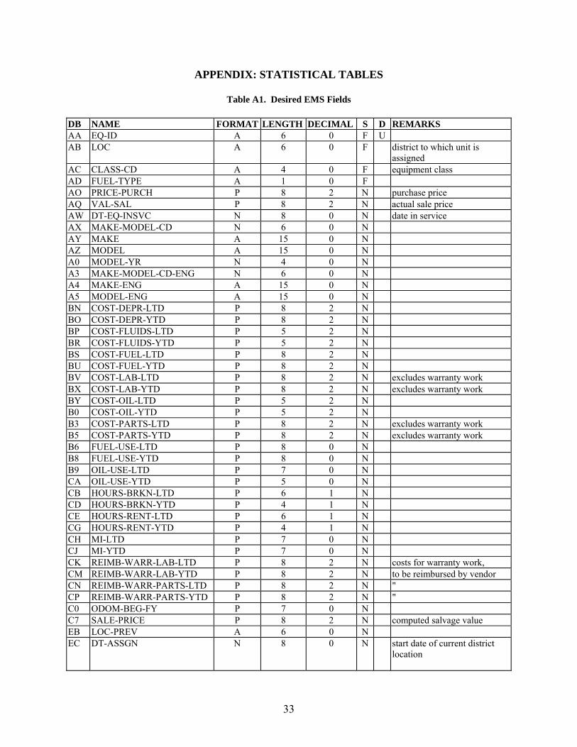
33

APPENDIX: STATISTICAL TABLES

Table A1. Desired EMS Fields DB NAME FORMAT LENGTH DECIMAL S D REMARKS AA EQ-ID A 6 0 F U AB LOC A 6 0 F district to which unit is

assigned AC CLASS-CD A 4 0 F equipment class AD FUEL-TYPE A 1 0 F AO PRICE-PURCH P 8 2 N purchase price AQ VAL-SAL P 8 2 N actual sale price AW DT-EQ-INSVC N 8 0 N date in service AX MAKE-MODEL-CD N 6 0 N AY MAKE A 15 0 N AZ MODEL A 15 0 N A0 MODEL-YR N 4 0 N A3 MAKE-MODEL-CD-ENG N 6 0 N A4 MAKE-ENG A 15 0 N A5 MODEL-ENG A 15 0 N BN COST-DEPR-LTD P 8 2 N BO COST-DEPR-YTD P 8 2 N BP COST-FLUIDS-LTD P 5 2 N BR COST-FLUIDS-YTD P 5 2 N BS COST-FUEL-LTD P 8 2 N BU COST-FUEL-YTD P 8 2 N BV COST-LAB-LTD P 8 2 N excludes warranty work BX COST-LAB-YTD P 8 2 N excludes warranty work BY COST-OIL-LTD P 5 2 N B0 COST-OIL-YTD P 5 2 N B3 COST-PARTS-LTD P 8 2 N excludes warranty work B5 COST-PARTS-YTD P 8 2 N excludes warranty work B6 FUEL-USE-LTD P 8 0 N B8 FUEL-USE-YTD P 8 0 N B9 OIL-USE-LTD P 7 0 N CA OIL-USE-YTD P 5 0 N CB HOURS-BRKN-LTD P 6 1 N CD HOURS-BRKN-YTD P 4 1 N CE HOURS-RENT-LTD P 6 1 N CG HOURS-RENT-YTD P 4 1 N CH MI-LTD P 7 0 N CJ MI-YTD P 7 0 N CK REIMB-WARR-LAB-LTD P 8 2 N costs for warranty work, CM REIMB-WARR-LAB-YTD P 8 2 N to be reimbursed by vendor CN REIMB-WARR-PARTS-LTD P 8 2 N " CP REIMB-WARR-PARTS-YTD P 8 2 N " C0 ODOM-BEG-FY P 7 0 N C7 SALE-PRICE P 8 2 N computed salvage value EB LOC-PREV A 6 0 N EC DT-ASSGN N 8 0 N start date of current district

location

34

EE ODOM-LATEST P 7 0 N odometer reading during latest accounting period

EH ODOM-BEG P 7 0 N odometer reading when first received

FB VAL-SURPLUS-EST P 8 2 N FE MFG-CD N 5 0 N FF DATE-MANUFACTURED N 8 0 N FQ WEIGHT-EMPTY-LBS P 6 0 N FR WEIGHT-GROSS-LBS P 6 0 N FS WEIGHT-NET-LBS P 6 0 N FT VDOT-LOAD-MAX-LBS P 6 0 N FU WHEEL-BASE-INCHES P 3 3 N FV TOWING-CAP-LBS P 6 0 N FW GAWF-LBS P 6 0 N gross axle weight, front FX GAWR-LBS P 6 0 N gross axle weight, rear HD COST-TOT-LTD-PREV P 8 2 N HE COST-TOT-YTD-PREV P 8 2 N HF HRS-RENT-LTD-PREV P 6 1 N HG HRS-RENT-YTD-PREV P 4 1 N

TOTALS 430

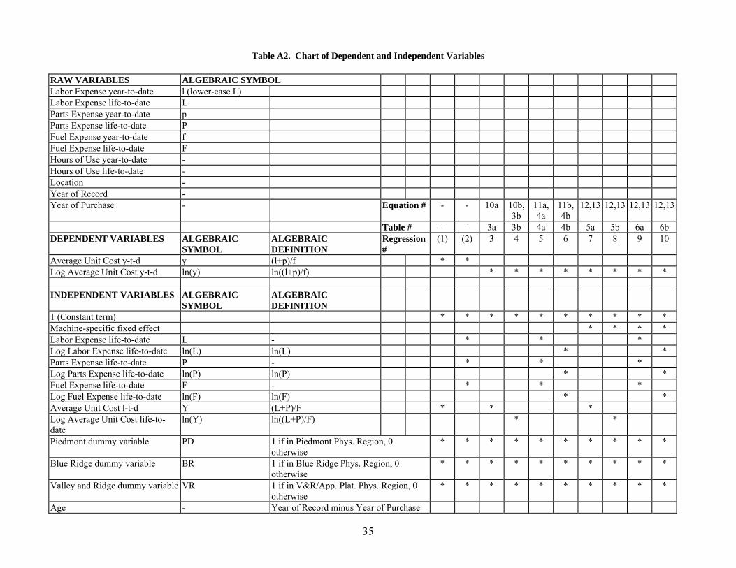
35

Table A2. Chart of Dependent and Independent Variables RAW VARIABLES ALGEBRAIC SYMBOL Labor Expense year-to-date l (lower-case L) Labor Expense life-to-date L Parts Expense year-to-date p Parts Expense life-to-date P Fuel Expense year-to-date f Fuel Expense life-to-date F Hours of Use year-to-date - Hours of Use life-to-date - Location - Year of Record - Year of Purchase - Equation # - - 10a 10b,

3b 11a,4a

11b,4b

12,13 12,13 12,13 12,13

Table # - - 3a 3b 4a 4b 5a 5b 6a 6b DEPENDENT VARIABLES ALGEBRAIC

SYMBOL ALGEBRAIC DEFINITION

Regression #

(1) (2) 3 4 5 6 7 8 9 10

Average Unit Cost y-t-d y (l+p)/f * * Log Average Unit Cost y-t-d ln(y) ln((l+p)/f) * * * * * * * *

INDEPENDENT VARIABLES ALGEBRAIC

SYMBOL ALGEBRAIC DEFINITION

1 (Constant term) * * * * * * * * * * Machine-specific fixed effect * * * * Labor Expense life-to-date L - * * * Log Labor Expense life-to-date ln(L) ln(L) * * Parts Expense life-to-date P - * * * Log Parts Expense life-to-date ln(P) ln(P) * * Fuel Expense life-to-date F - * * * Log Fuel Expense life-to-date ln(F) ln(F) * * Average Unit Cost l-t-d Y (L+P)/F * * * Log Average Unit Cost life-to-date

ln(Y) ln((L+P)/F) * *

Piedmont dummy variable PD 1 if in Piedmont Phys. Region, 0 otherwise

* * * * * * * * * *

Blue Ridge dummy variable BR 1 if in Blue Ridge Phys. Region, 0 otherwise

* * * * * * * * * *

Valley and Ridge dummy variable VR 1 if in V&R/App. Plat. Phys. Region, 0 otherwise

* * * * * * * * * *

Age - Year of Record minus Year of Purchase

36

Table A3. Results of Pooled Regression: Equation 10a, Log-Linear Specification

285 286 336 338 340Beta 1 (Constant) 0.5699 0.6871 1.2543 0.9041 0.4099

-6.2039 6.6640 8.5093 9.4039 1.1622Beta 2 (Y(t-1)) 0.2459 0.2190 0.0979 0.1590 0.2814

9.1483 8.9481 2.7200 8.0615 4.1242Beta 3 (VR dummy) -0.0963 0.0684 -0.3739 -0.1077 0.1299

-1.0800 0.6599 -1.7140 -1.1756 0.3776Beta 4 (BR dummy) -0.1745 0.1404 -0.3716 -0.1785 0.3960

-1.9194 1.3227 -2.2245 -1.7764 0.6976Beta 5 (PD dummy) -0.4687 0.2458 0.1667 -0.0033 0.5483

-5.2427 2.4646 1.0870 -0.0353 1.1209Sample Size 780 779 244 1,106 94R-Squared 0.1468 0.1075 0.0861 0.0633 0.2121

824 828 864 866 896

Beta 1 (Constant) 0.3604 0.3422 0.9451 0.2766 0.6884 11.1990 13.2070 37.5913 3.7834 10.9680

Beta 2 (Y(t-1)) -0.0496 -0.0322 0.0135 -0.0075 0.1330 -8.3259 -6.4125 8.9223 -0.7647 6.7010

Beta 3 (VR dummy) -0.1510 -0.1679 -0.0712 0.4020 -0.2644 -3.2184 -4.1573 -2.0929 3.9881 -3.9615

Beta 4 (BR dummy) -0.0424 -0.1379 -0.2422 0.4176 -0.1634 -0.7190 -3.1232 -6.3521 3.3068 -2.0812

Beta 5 (PD dummy) -0.0385 0.1182 0.0071 0.4073 -0.0364 -0.9600 3.4007 0.2199 3.9087 -0.5449

Sample Size 3,227 3,746 6,663 680 1,205R-Squared 0.0241 0.0256 0.0204 0.0331 0.0505

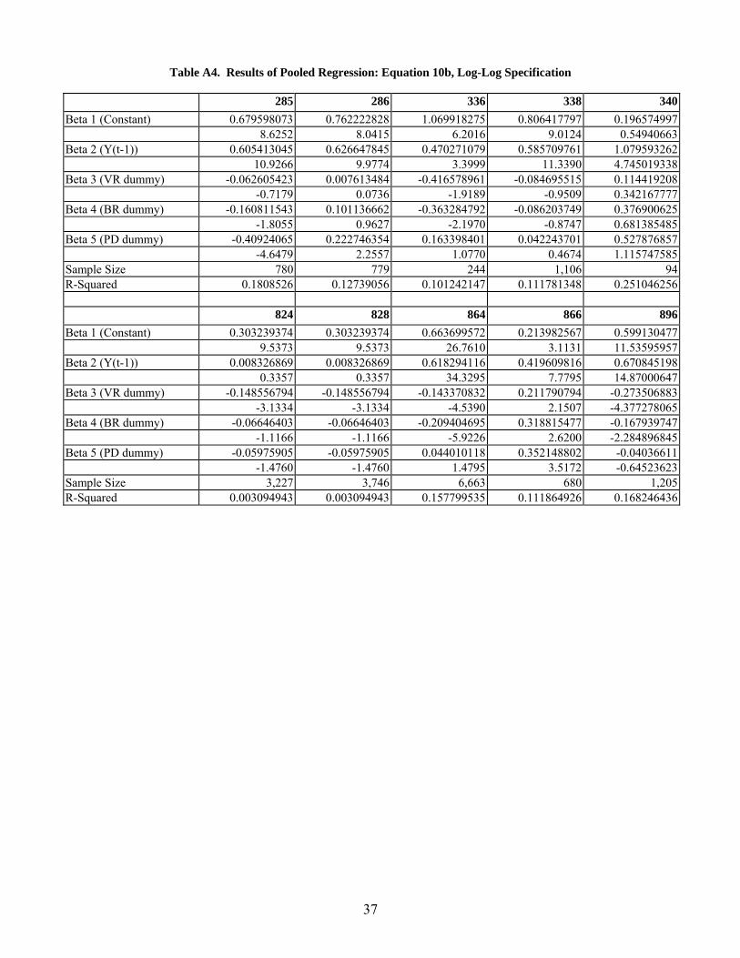
37

Table A4. Results of Pooled Regression: Equation 10b, Log-Log Specification

285 286 336 338 340Beta 1 (Constant) 0.679598073 0.762222828 1.069918275 0.806417797 0.196574997

8.6252 8.0415 6.2016 9.0124 0.54940663Beta 2 (Y(t-1)) 0.605413045 0.626647845 0.470271079 0.585709761 1.079593262

10.9266 9.9774 3.3999 11.3390 4.745019338Beta 3 (VR dummy) -0.062605423 0.007613484 -0.416578961 -0.084695515 0.114419208

-0.7179 0.0736 -1.9189 -0.9509 0.342167777Beta 4 (BR dummy) -0.160811543 0.101136662 -0.363284792 -0.086203749 0.376900625

-1.8055 0.9627 -2.1970 -0.8747 0.681385485Beta 5 (PD dummy) -0.40924065 0.222746354 0.163398401 0.042243701 0.527876857

-4.6479 2.2557 1.0770 0.4674 1.115747585Sample Size 780 779 244 1,106 94R-Squared 0.1808526 0.12739056 0.101242147 0.111781348 0.251046256

824 828 864 866 896

Beta 1 (Constant) 0.303239374 0.303239374 0.663699572 0.213982567 0.599130477 9.5373 9.5373 26.7610 3.1131 11.53595957

Beta 2 (Y(t-1)) 0.008326869 0.008326869 0.618294116 0.419609816 0.670845198 0.3357 0.3357 34.3295 7.7795 14.87000647

Beta 3 (VR dummy) -0.148556794 -0.148556794 -0.143370832 0.211790794 -0.273506883 -3.1334 -3.1334 -4.5390 2.1507 -4.377278065

Beta 4 (BR dummy) -0.06646403 -0.06646403 -0.209404695 0.318815477 -0.167939747 -1.1166 -1.1166 -5.9226 2.6200 -2.284896845

Beta 5 (PD dummy) -0.05975905 -0.05975905 0.044010118 0.352148802 -0.04036611 -1.4760 -1.4760 1.4795 3.5172 -0.64523623

Sample Size 3,227 3,746 6,663 680 1,205R-Squared 0.003094943 0.003094943 0.157799535 0.111864926 0.168246436

38

Table A5. Results of Pooled Regression: Equation 11a, Log-Linear Specification

285 286 336 338 340Beta 1 (Constant) 0.79494890 1.03371909 1.63610447 1.11172570 0.82541043

8.84199 10.53982 9.55045 13.32281 1.97839Beta 2 (L(t-1)) 0.00002923 0.00003073 0.00001402 0.00004576 0.00005563

4.29350 3.74450 0.79092 5.01476 1.21959Beta 3 (P(t-1)) 0.00000925 0.00000769 0.00001260 0.00001668 0.00001729

2.23746 2.23319 1.48733 3.23036 1.13141Beta 4 (F(t-1)) -0.00000812 -0.00001195 -0.00004824 -0.00001565 -0.00003754

-1.04170 -1.27915 -2.06603 -1.31731 -0.95983Beta 5 (VR dummy) -0.11831304 -0.06142620 -0.37274445 -0.36326314 0.06829793

-1.31227 -0.55104 -1.53020 -3.86742 0.17749Beta 6 (BR dummy) -0.23193696 -0.00085215 -0.35476840 -0.31116976 0.36852591

-2.48952 -0.00747 -2.06563 -3.12879 0.61964Beta 7 (PD dummy) -0.41255849 0.25640816 0.17531548 -0.10899213 0.89100591

-4.53741 2.54215 1.13085 -1.20103 1.75555Sample Size 780 779 244 1,106 94R-Squared 0.141800841 0.101649392 0.083971921 0.10039195 0.214536941

824 828 864 866 896

Beta 1 (Constant) -0.15112986 -0.04299728 0.55853020 -0.15075545 0.56192128 -3.95696 -1.44761 20.11716 -2.00004 11.42633

Beta 2 (L(t-1)) 0.00000940 0.00004332 0.00003868 0.00006256 0.00002543 0.46496 3.07495 8.92351 4.22942 4.43756

Beta 3 (P(t-1)) 0.00009574 0.00006761 0.00004075 0.00002098 0.00002058 6.89633 7.30442 13.30907 2.26100 4.39219

Beta 4 (F(t-1)) 0.00005392 0.00003001 -0.00001378 0.00000746 -0.00000227 4.96651 3.50749 -3.12329 0.58331 -0.37642

Beta 5 (VR dummy) -0.07034557 -0.18340010 -0.29209538 0.00324449 -0.39575574 -1.56470 -4.76190 -9.29952 0.03527 -6.59324

Beta 6 (BR dummy) -0.05903479 -0.19008525 -0.27013945 -0.00843121 -0.34457279 -1.04967 -4.49354 -7.79190 -0.07255 -4.78509

Beta 7 (PD dummy) 0.03297851 0.07449533 0.01107271 0.34474714 -0.10875856 0.84763 2.24493 0.37939 3.76209 -1.82804

Sample Size 3,227 3,746 6,663 680 1,205R-Squared 0.113132142 0.120893098 0.19540217 0.257653825 0.260521748

39

Table A6. Results of Pooled Regression: Equation 11b, Log-Log Specification

285 286 336 338 340Beta 1 (Constant) -0.453956639 0.058674359 1.953753268 -0.426210686 -3.013780295

-1.33226 0.12435 1.75910 -1.54808 -1.79027Beta 2 (L(t-1)) 0.149105344 0.344415814 0.084836215 0.286462624 0.784421804

2.76591 4.94941 0.47188 5.31443 1.70363Beta 3 (P(t-1)) 0.354898463 0.249442076 0.355472847 0.234719634 0.260654826

5.85443 3.50729 2.32065 4.68206 0.60413Beta 4 (F(t-1)) -0.338522751 -0.447239058 -0.50814564 -0.306229412 -0.583368514

-4.37205 -4.26810 -2.84039 -4.68212 -1.87518Beta 5 (VR dummy) -0.049980271 -0.128260721 -0.394809716 -0.269977432 0.336361383

-0.58733 -1.17831 -1.71149 -2.94652 0.78265Beta 6 (BR dummy) -0.159449801 -0.029776359 -0.332148182 -0.213101147 0.307970888

-1.81424 -0.27014 -1.92782 -2.15183 0.55272Beta 7 (PD dummy) -0.368884548 0.230548378 0.153801217 -0.036363984 0.920718721

-4.28133 2.33366 0.97822 -0.40677 1.68123Sample Size 780 779 244 1,106 94R-Squared 0.222525226 0.14414207 0.104655973 0.142464251 0.299252267

824 828 864 866 896

Beta 1 (Constant) -2.528092853 -2.528092853 -1.58058958 -2.538201031 -1.966219128 -23.02366 -23.02366 -20.48904 -11.61993 -12.39859

Beta 2 (L(t-1)) 0.125845242 0.125845242 0.371653032 0.266922593 0.329141563 3.99245 3.99245 14.92262 3.50121 7.30656

Beta 3 (P(t-1)) 0.109214538 0.109214538 0.290960152 0.25197328 0.159904782 5.60233 5.60233 13.60908 3.54812 3.68179

Beta 4 (F(t-1)) 0.146360751 0.146360751 -0.341724065 -0.136447654 -0.132305549 5.44435 5.44435 -18.58566 -2.69610 -2.82851

Beta 5 (VR dummy) -0.117111101 -0.117111101 -0.218340078 -0.016689509 -0.407674245 -2.74940 -2.74940 -7.53478 -0.19394 -7.56078

Beta 6 (BR dummy) -0.084150892 -0.084150892 -0.204369873 -0.086363212 -0.355809209 -1.56761 -1.56761 -6.34290 -0.78913 -5.59412

Beta 7 (PD dummy) 0.068891256 0.068891256 0.030056907 0.178734994 -0.121741734 1.87745 1.87745 1.10303 2.05262 -2.23515

Sample Size 3,227 3,746 6,663 680 1,205R-Squared 0.196425284 0.196425284 0.30167089 0.342916018 0.393752245

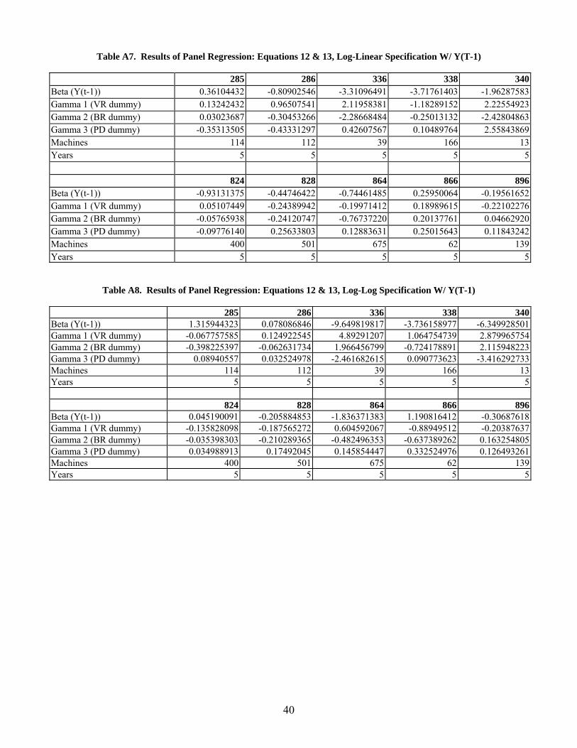
40

Table A7. Results of Panel Regression: Equations 12 & 13, Log-Linear Specification W/ Y(T-1)

285 286 336 338 340Beta (Y(t-1)) 0.36104432 -0.80902546 -3.31096491 -3.71761403 -1.96287583Gamma 1 (VR dummy) 0.13242432 0.96507541 2.11958381 -1.18289152 2.22554923Gamma 2 (BR dummy) 0.03023687 -0.30453266 -2.28668484 -0.25013132 -2.42804863Gamma 3 (PD dummy) -0.35313505 -0.43331297 0.42607567 0.10489764 2.55843869Machines 114 112 39 166 13Years 5 5 5 5 5

824 828 864 866 896

Beta (Y(t-1)) -0.93131375 -0.44746422 -0.74461485 0.25950064 -0.19561652Gamma 1 (VR dummy) 0.05107449 -0.24389942 -0.19971412 0.18989615 -0.22102276Gamma 2 (BR dummy) -0.05765938 -0.24120747 -0.76737220 0.20137761 0.04662920Gamma 3 (PD dummy) -0.09776140 0.25633803 0.12883631 0.25015643 0.11843242Machines 400 501 675 62 139Years 5 5 5 5 5

Table A8. Results of Panel Regression: Equations 12 & 13, Log-Log Specification W/ Y(T-1)

285 286 336 338 340Beta (Y(t-1)) 1.315944323 0.078086846 -9.649819817 -3.736158977 -6.349928501Gamma 1 (VR dummy) -0.067757585 0.124922545 4.89291207 1.064754739 2.879965754Gamma 2 (BR dummy) -0.398225397 -0.062631734 1.966456799 -0.724178891 2.115948223Gamma 3 (PD dummy) 0.08940557 0.032524978 -2.461682615 0.090773623 -3.416292733Machines 114 112 39 166 13Years 5 5 5 5 5

824 828 864 866 896

Beta (Y(t-1)) 0.045190091 -0.205884853 -1.836371383 1.190816412 -0.30687618Gamma 1 (VR dummy) -0.135828098 -0.187565272 0.604592067 -0.88949512 -0.20387637Gamma 2 (BR dummy) -0.035398303 -0.210289365 -0.482496353 -0.637389262 0.163254805Gamma 3 (PD dummy) 0.034988913 0.17492045 0.145854447 0.332524976 0.126493261Machines 400 501 675 62 139Years 5 5 5 5 5

41

Table A9. Results of Panel Regression: Equations 12 & 13, Log-Linear Specification W/L, P, F

285 286 336 338 340Beta 1 (L(t-1)) -0.00006030 0.00009893 -0.00066352 -0.00004637 0.00024287Beta 2 (P(t-1)) -0.00011303 -0.00045772 -0.00064295 -0.00112214 -0.00024494Beta 3 (F(t-1)) 0.00072560 0.00185560 0.00327116 0.00421111 0.00214786Gamma 1 (VR dummy) -0.15543019 -0.08722839 1.61738353 -6.54913038 -3.41428493Gamma 2 (BR dummy) -0.50215106 -3.23817755 -5.51488235 1.11744171 -12.25326666Gamma 3 (PD dummy) -0.18590229 1.97922358 1.80824475 2.38889096 12.23672330Machines 114 112 39 166 13Years 5 5 5 5 5

824 828 864 866 896

Beta 1 (L(t-1)) -0.00056773 -0.00033529 0.00048366 0.00139991 0.00004651Beta 2 (P(t-1)) -0.00086908 -0.00046950 -0.00006526 -0.00077654 -0.00019288Beta 3 (F(t-1)) 0.00156698 0.00098338 0.00019029 0.00021670 0.00043540Gamma 1 (VR dummy) 0.54823573 -0.41669085 -0.98526359 -2.77746397 -0.25294501Gamma 2 (BR dummy) -1.08913665 -0.57420731 -0.18053121 -3.24991765 -1.11944372Gamma 3 (PD dummy) 0.50107615 0.60620132 0.47669699 1.54528661 0.11171786Machines 400 501 675 62 139Years 5 5 5 5 5

Table A10. Results of Panel Regression: Equations 12 & 13, Log-Log Specification W/L, P, F

285 286 336 338 340Beta 1 (L(t-1)) 2.672907873 -0.237164434 -3.380854723 -3.310979232 12.43520967Beta 2 (P(t-1)) -1.450946774 -3.78655686 -14.40993296 -4.759491351 -20.42228816Beta 3 (F(t-1)) 1.281222527 10.96752735 33.48699811 16.49434188 36.54647283Gamma 1 (VR dummy) 0.125503954 -1.048900017 -1.671191384 -3.538810006 0.531350776Gamma 2 (BR dummy) -1.151868514 -1.483504522 -7.681731258 0.257076553 -19.9566081Gamma 3 (PD dummy) 0.334468362 1.316215876 3.933325722 0.100938014 25.51568147Machines 114 112 39 166 13Years 5 5 5 5 5

824 828 864 866 896

Beta 1 (L(t-1)) -0.010398101 0.273447086 -6.581506798 1.80666296 0.667125969Beta 2 (P(t-1)) -0.316580441 -0.534636808 0.453570769 -0.71111002 -0.284524914Gamma 1 (VR dummy) 0.040598946 -0.31253347 -1.694882368 -0.73884430 -0.205793128Gamma 2 (BR dummy) -0.321228818 -0.310421036 -0.552031273 -0.72408053 -0.23352096Gamma 3 (PD dummy) 0.235676819 0.363285175 -0.073947164 0.32319933 0.120312616Machines 400 501 675 62 139Years 5 5 5 5 5