Final Report Template - mla.com.au
66
final re p port Project code: P.PIP.0290 2011 Prepared by: Drs. Bronwen Butler and Michael Johns Johns Environmental Date submitted: August 2012 PUBLISHED BY Meat & Livestock Australia Limited Locked Bag 991 NORTH SYDNEY NSW 2059 Demonstration of Covered Anaerobic Pond Technology Meat & Livestock Australia and the MLA Donor Company acknowledge the matching funds provided by the Australian Government and contributions from the Australian Meat Processor Corporation to support the research and development detailed in this publication. This publication is published by Meat & Livestock Australia Limited ABN 39 081 678 364 (MLA). Care is taken to ensure the accuracy of the information contained in this publication. However MLA cannot accept responsibility for the accuracy or completeness of the information or opinions contained in the publication. You should make your own enquiries before making decisions concerning your interests. Reproduction in whole or in part of this publication is prohibited without prior written consent of MLA.
Transcript of Final Report Template - mla.com.au
final repport
Project code: P.PIP.0290 2011
Prepared by: Drs. Bronwen Butler and Michael Johns
Johns Environmental
Date submitted: August 2012
PUBLISHED BY Meat & Livestock Australia Limited Locked Bag 991 NORTH SYDNEY NSW 2059
Demonstration of Covered Anaerobic Pond Technology
Meat & Livestock Australia and the MLA Donor Company acknowledge the matching funds provided by the Australian Government and contributions from the Australian Meat Processor Corporation to support the research and development detailed in this publication.
This publication is published by Meat & Livestock Australia Limited ABN 39 081 678 364 (MLA). Care is taken to ensure the accuracy of the information contained in this publication. However MLA cannot accept responsibility for the accuracy or completeness of the information or opinions contained in the publication. You should make your own enquiries before making decisions concerning your interests. Reproduction in whole or in part of this publication is prohibited without prior written consent of MLA.
Page 1 of 66
P.PIP.0290 - Demonstration of Covered Anaerobic Pond Technology
Abstract
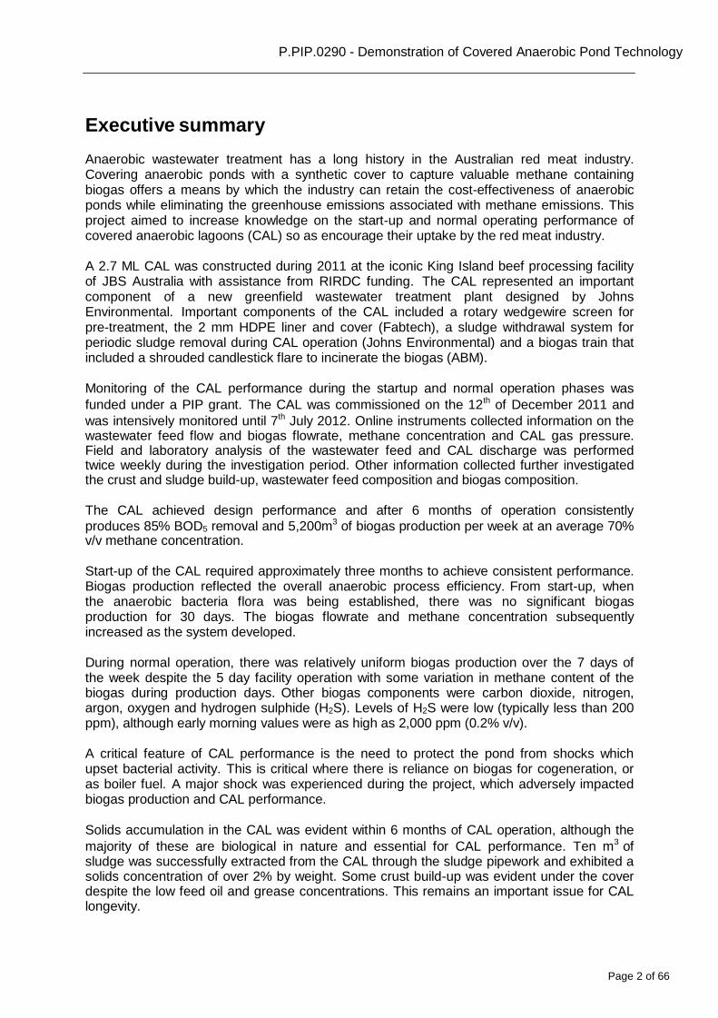
Capturing biogas from covered anaerobic lagoons (CALs) provides a valuable fuel source and greatly reduces carbon emissions. This project aimed to increase knowledge on the start-up and normal operating performance of covered anaerobic lagoons (CAL) so as encourage their uptake by the red meat industry.
CAL performance was assessed by intensive monitoring of the 2.7 ML CAL at JBS Australia’s King Island facility for 7 months from commissioning. The CAL started up successfully and showed steady state operation within 6 months. The results show biogas production and quality was affected significantly by many factors. One of the measures used to successfully gauge the health of the CAL was the ratio of volatile fatty acids to total alkalinity. There is a wealth of valuable insight in this report.
Page 2 of 66
P.PIP.0290 - Demonstration of Covered Anaerobic Pond Technology
Executive summary
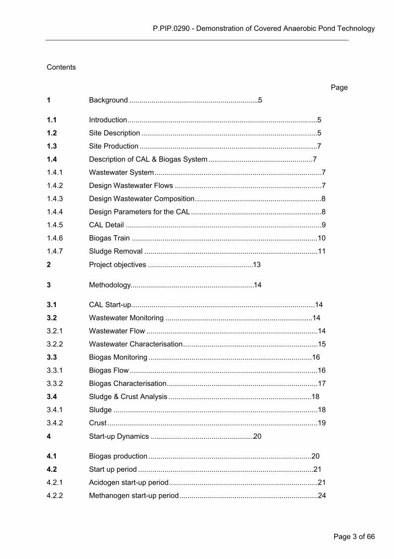
Anaerobic wastewater treatment has a long history in the Australian red meat industry. Covering anaerobic ponds with a synthetic cover to capture valuable methane containing biogas offers a means by which the industry can retain the cost-effectiveness of anaerobic ponds while eliminating the greenhouse emissions associated with methane emissions. This project aimed to increase knowledge on the start-up and normal operating performance of covered anaerobic lagoons (CAL) so as encourage their uptake by the red meat industry.
A 2.7 ML CAL was constructed during 2011 at the iconic King Island beef processing facility of JBS Australia with assistance from RIRDC funding. The CAL represented an important component of a new greenfield wastewater treatment plant designed by Johns Environmental. Important components of the CAL included a rotary wedgewire screen for pre-treatment, the 2 mm HDPE liner and cover (Fabtech), a sludge withdrawal system for periodic sludge removal during CAL operation (Johns Environmental) and a biogas train that included a shrouded candlestick flare to incinerate the biogas (ABM).
Monitoring of the CAL performance during the startup and normal operation phases was
funded under a PIP grant. The CAL was commissioned on the 12th of December 2011 and
was intensively monitored until 7th July 2012. Online instruments collected information on the wastewater feed flow and biogas flowrate, methane concentration and CAL gas pressure. Field and laboratory analysis of the wastewater feed and CAL discharge was performed twice weekly during the investigation period. Other information collected further investigated the crust and sludge build-up, wastewater feed composition and biogas composition.
The CAL achieved design performance and after 6 months of operation consistently
produces 85% BOD5 removal and 5,200m3 of biogas production per week at an average 70% v/v methane concentration.
Start-up of the CAL required approximately three months to achieve consistent performance. Biogas production reflected the overall anaerobic process efficiency. From start-up, when the anaerobic bacteria flora was being established, there was no significant biogas production for 30 days. The biogas flowrate and methane concentration subsequently increased as the system developed.
During normal operation, there was relatively uniform biogas production over the 7 days of the week despite the 5 day facility operation with some variation in methane content of the biogas during production days. Other biogas components were carbon dioxide, nitrogen, argon, oxygen and hydrogen sulphide (H2S). Levels of H2S were low (typically less than 200 ppm), although early morning values were as high as 2,000 ppm (0.2% v/v).
A critical feature of CAL performance is the need to protect the pond from shocks which upset bacterial activity. This is critical where there is reliance on biogas for cogeneration, or as boiler fuel. A major shock was experienced during the project, which adversely impacted biogas production and CAL performance.
Solids accumulation in the CAL was evident within 6 months of CAL operation, although the
majority of these are biological in nature and essential for CAL performance. Ten m3 of sludge was successfully extracted from the CAL through the sludge pipework and exhibited a solids concentration of over 2% by weight. Some crust build-up was evident under the cover despite the low feed oil and grease concentrations. This remains an important issue for CAL longevity.
Page 3 of 66
P.PIP.0290 - Demonstration of Covered Anaerobic Pond Technology
Contents
Page
1 Background ................................................................ 5
1.1 Introduction .............................................................................................5
1.2 Site Description ......................................................................................5
1.3 Site Production .......................................................................................7
1.4 Description of CAL & Biogas System ...................................................7
1.4.1 Wastewater System ..................................................................................7
1.4.2 Design Wastewater Flows ........................................................................7
1.4.3 Design Wastewater Composition ..............................................................8
1.4.4 Design Parameters for the CAL ................................................................8
1.4.5 CAL Detail ................................................................................................9
1.4.6 Biogas Train ........................................................................................... 10
1.4.7 Sludge Removal ..................................................................................... 11
2 Project objectives .................................................... 13
3 Methodology ............................................................. 14
3.1 CAL Start-up .......................................................................................... 14
3.2 Wastewater Monitoring ........................................................................ 14
3.2.1 Wastewater Flow .................................................................................... 14
3.2.2 Wastewater Characterisation .................................................................. 15
3.3 Biogas Monitoring ................................................................................ 16
3.3.1 Biogas Flow ............................................................................................ 16
3.3.2 Biogas Characterisation .......................................................................... 17
3.4 Sludge & Crust Analysis ...................................................................... 18
3.4.1 Sludge .................................................................................................... 18
3.4.2 Crust ....................................................................................................... 19
4 Start-up Dynamics ................................................... 20
4.1 Biogas production ................................................................................ 20
4.2 Start up period ...................................................................................... 21
4.2.1 Acidogen start-up period ......................................................................... 21
4.2.2 Methanogen start-up period .................................................................... 24
Page 4 of 66
P.PIP.0290 - Demonstration of Covered Anaerobic Pond Technology
4.3 Influence of shocks (perturbations) .................................................... 26
4.4 Microbial Stress Indicators .................................................................. 28
4.5 Pond Temperature ................................................................................ 29
5 Normal Operating Performance .............................. 30
5.1 Biogas production ................................................................................ 30
5.1.1 Biogas flowrate ....................................................................................... 30
5.1.2 Biogas methane composition .................................................................. 31
5.1.3 Biogas composition – other components ................................................ 33
5.2 Contaminant Removal from the Wastewater ...................................... 36
5.2.1 Influent Composition ............................................................................... 36
5.2.2 COD and BOD5 removal by the CAL ...................................................... 39
5.2.3 TSS and Oil & Grease Removal ............................................................. 40
5.2.4 Feed Flow ............................................................................................... 41
5.3 Estimate of Biogas Production ............................................................ 42
6 Crust & Solids accumulation .................................. 43
6.1 Crust Build-up ....................................................................................... 43
6.2 Sludge Accumulation ........................................................................... 44
7 Conclusions .............................................................. 46
8 Recommendations ................................................... 47
Page 5 of 66
P.PIP.0290 - Demonstration of Covered Anaerobic Pond Technology
1 Background
1.1 Introduction
Anaerobic ponds (without synthetic covers) have long been the cornerstone of meat processing wastewater treatment systems. They provide robust and cost-effective removal of organic loads and their natural tendency to form floating crusts helped minimise odour emissions. However the large quantity of methane-rich biogas emitted from these ponds forms a significant contribution towards direct Scope 1 greenhouse gas (GHG) emissions from meat processing facilities and represents lost fuel value.
Many proprietary high rate anaerobic systems have been installed in industrial wastewater systems and offer the capacity to capture the biogas. Unfortunately these have a poor record with meat processing wastewater largely because of the tendency of high oil & grease and total suspended solids concentrations to interfere with microbial granulation, which is generally critical for successful high rate system function.
The emergence of CALs provides a more appropriate fit for meat processing wastewater. Considerable unknowns and risks exist for CAL technology implementation in the meat processing sector including:
unknown start-up behaviour of anaerobic systems at green field sites;
limited data regarding biogas production rates and quality;
the danger of crust accumulation under the cover causing mechanical damage and eventually cover failure.
The King Island meat processing site owned by JBS Australia Pty Ltd. (JBS) was selected as an ideal demonstration site due to its unique environment. The Rural Industries Research and Development Corporation (RIRDC) contributed capital funding to assist JBS to construct a new CAL with instrumentation and technologies required to demonstrate and monitor its effectiveness. The Australian Meat Processor Corporation (AMPC), Meat & Livestock Australia (MLA) and JBS provided funding to conduct a 9 month research PIP program to monitor the startup and normal operation of the CAL.
This demonstration site and the associated monitoring research project is a first step in ensuring that the red meat processing sector is best placed to develop a suite of strategies and tools able to equip the industry to meet the challenges faced in responding to climate change and to capitalise on opportunities that invariably accompany fundamental change of this magnitude.
1.2 Site Description
King Island, located between Victoria and Tasmania, has a population of approximately 1300 residents. There are about 85,000 head of cattle on the island being 30% dairy and 70% beef. The King Island Abattoir facility was originally built by the Tasmanian Government in the 1950’s. In May 2008, JBS acquired the King Island site which currently employs 85 people. JBS have 10 abattoirs throughout Australia, with the King Island site contributing to approximately 1.6% of the weekly beef processing capacity.
Page 6 of 66
P.PIP.0290 - Demonstration of Covered Anaerobic Pond Technology
King Island
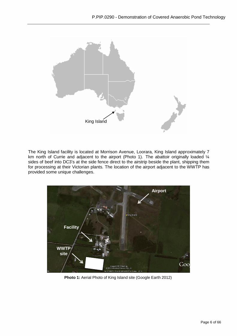
The King Island facility is located at Morrison Avenue, Loorara, King Island approximately 7 km north of Currie and adjacent to the airport (Photo 1). The abattoir originally loaded ¼ sides of beef into DC3’s at the side fence direct to the airstrip beside the plant, shipping them for processing at their Victorian plants. The location of the airport adjacent to the WWTP has provided some unique challenges.
Airport
Facility
WWTP
site
Photo 1: Aerial Photo of King Island site (Google Earth 2012)
Page 7 of 66
P.PIP.0290 - Demonstration of Covered Anaerobic Pond Technology
1.3 Site Production
The abattoir comprises a beef processing floor which typically operates 5 days/week, 235 days/year processing up to 180 head of cattle per day, on a single kill shift basis with 1 boning shift. There exists a full range of ancillary operations including rendering (HTR), boning and offal and intestine processing. Hides from the processed cattle are dry salted for off-site transport.
Although the abattoir is small relative to most in Australia, it is representative of the larger facilities in being fully integrated and having a full suite of ancillary operations.
1.4 Description of CAL & Biogas System
The CAL was designed by Johns Environmental Pty Ltd [JEPL] as the first of several ponds in a greenfield pond-based wastewater treatment system. The design reflects 20 years experience of the company with anaerobic ponds in the meat processing industry. This section gives an overview of the CAL design for the JBS Australia King Island facility.
1.4.1 Wastewater System
The CAL formed one part of a greenfield WWTP comprising:
1 new raw wastewater pump pit, pumps and rising main;
A new rotary screen to provide fine and gross solids removal. An old DAF wasdecommissioned and not replaced due to relatively low oil & grease levels in the rawwastewater;
1 new 2.7 ML CAL with biogas train and flare;
Downstream aerated pond with ancillary settle basin and two aerobic polishing ponds.
This project focussed on the new CAL.
1.4.2 Design Wastewater Flows
The major flow is generated on production days. The CAL was designed to handle a production design average flow of 290 kL/day Mon-Fri. This includes some wet weather capture.
Page 8 of 66
P.PIP.0290 - Demonstration of Covered Anaerobic Pond Technology
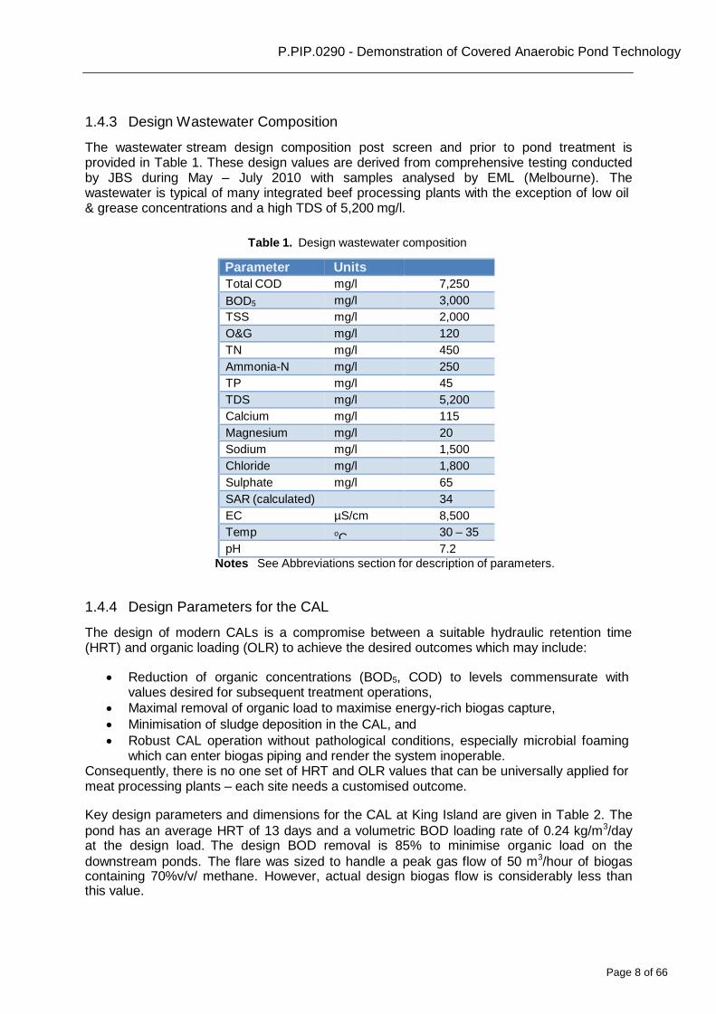
1.4.3 Design Wastewater Composition
The wastewater stream design composition post screen and prior to pond treatment is provided in Table 1. These design values are derived from comprehensive testing conducted by JBS during May – July 2010 with samples analysed by EML (Melbourne). The wastewater is typical of many integrated beef processing plants with the exception of low oil & grease concentrations and a high TDS of 5,200 mg/l.
Table 1. Design wastewater composition
Parameter Units Total COD mg/l 7,250
BOD5 mg/l 3,000
TSS mg/l 2,000
O&G mg/l 120
TN mg/l 450
Ammonia-N mg/l 250
TP mg/l 45
TDS mg/l 5,200
Calcium mg/l 115
Magnesium mg/l 20
Sodium mg/l 1,500
Chloride mg/l 1,800
Sulphate mg/l 65
SAR (calculated) 34
EC µS/cm 8,500
Temp oC 30 – 35
pH 7.2
Notes See Abbreviations section for description of parameters.
1.4.4 Design Parameters for the CAL
The design of modern CALs is a compromise between a suitable hydraulic retention time (HRT) and organic loading (OLR) to achieve the desired outcomes which may include:
Reduction of organic concentrations (BOD5, COD) to levels commensurate with
values desired for subsequent treatment operations,
Maximal removal of organic load to maximise energy-rich biogas capture,
Minimisation of sludge deposition in the CAL, and
Robust CAL operation without pathological conditions, especially microbial foaming which can enter biogas piping and render the system inoperable.
Consequently, there is no one set of HRT and OLR values that can be universally applied for meat processing plants – each site needs a customised outcome.
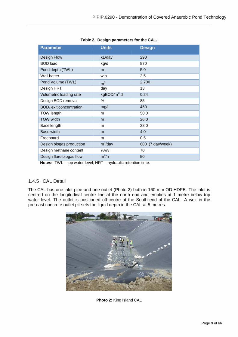
Key design parameters and dimensions for the CAL at King Island are given in Table 2. The
pond has an average HRT of 13 days and a volumetric BOD loading rate of 0.24 kg/m3/day at the design load. The design BOD removal is 85% to minimise organic load on the
downstream ponds. The flare was sized to handle a peak gas flow of 50 m3/hour of biogas containing 70%v/v/ methane. However, actual design biogas flow is considerably less than this value.
Page 9 of 66
P.PIP.0290 - Demonstration of Covered Anaerobic Pond Technology
Table 2. Design parameters for the CAL.
Parameter Units Design
Design Flow kL/day 290
BOD load kg/d 870
Pond depth (TWL) m 5.0
Wall batter w:h 2.5
Pond Volume (TWL) m3 2,700
Design HRT day 13
Volumetric loading rate kgBOD/m3.d 0.24
Design BOD removal % 85
BOD5 exit concentration mg/l 450
TOW length m 50.0
TOW width m 26.0
Base length m 28.0
Base width m 4.0
Freeboard m 0.5
Design biogas production m3/day 600 (7 day/week)
Design methane content %v/v 70
Design flare biogas flow m3/h 50
Notes: TWL – top water level; HRT – hydraulic retention time.
1.4.5 CAL Detail
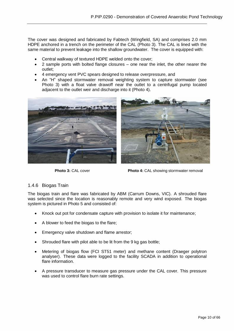
The CAL has one inlet pipe and one outlet (Photo 2) both in 160 mm OD HDPE. The inlet is centred on the longitudinal centre line at the north end and empties at 1 metre below top water level. The outlet is positioned off-centre at the South end of the CAL. A weir in the pre-cast concrete outlet pit sets the liquid depth in the CAL at 5 metres.
Photo 2: King Island CAL
Page 10 of 66
P.PIP.0290 - Demonstration of Covered Anaerobic Pond Technology
The cover was designed and fabricated by Fabtech (Wingfield, SA) and comprises 2.0 mm HDPE anchored in a trench on the perimeter of the CAL (Photo 3). The CAL is lined with the same material to prevent leakage into the shallow groundwater. The cover is equipped with:
Central walkway of textured HDPE welded onto the cover;
2 sample ports with bolted flange closures – one near the inlet, the other nearer the outlet;
4 emergency vent PVC spears designed to release overpressure, and
An “H” shaped stormwater removal weighting system to capture stormwater (see Photo 3) with a float valve drawoff near the outlet to a centrifugal pump located adjacent to the outlet weir and discharge into it (Photo 4).
Photo 3: CAL cover Photo 4: CAL showing stormwater removal
1.4.6 Biogas Train
The biogas train and flare was fabricated by ABM (Carrum Downs, VIC). A shrouded flare was selected since the location is reasonably remote and very wind exposed. The biogas system is pictured in Photo 5 and consisted of:
Knock out pot for condensate capture with provision to isolate it for maintenance;
A blower to feed the biogas to the flare;
Emergency valve shutdown and flame arrestor;
Shrouded flare with pilot able to be lit from the 9 kg gas bottle;
Metering of biogas flow (FCI ST51 meter) and methane content (Draeger polytron analyser). These data were logged to the facility SCADA in addition to operational flare information.
A pressure transducer to measure gas pressure under the CAL cover. This pressure
was used to control flare burn rate settings.
Page 11 of 66
P.PIP.0290 - Demonstration of Covered Anaerobic Pond Technology
Photo 5: Biogas train
The original intent for JBS was to run a small (30 kWe) gas engine, but the decision to install this has been put on hold.
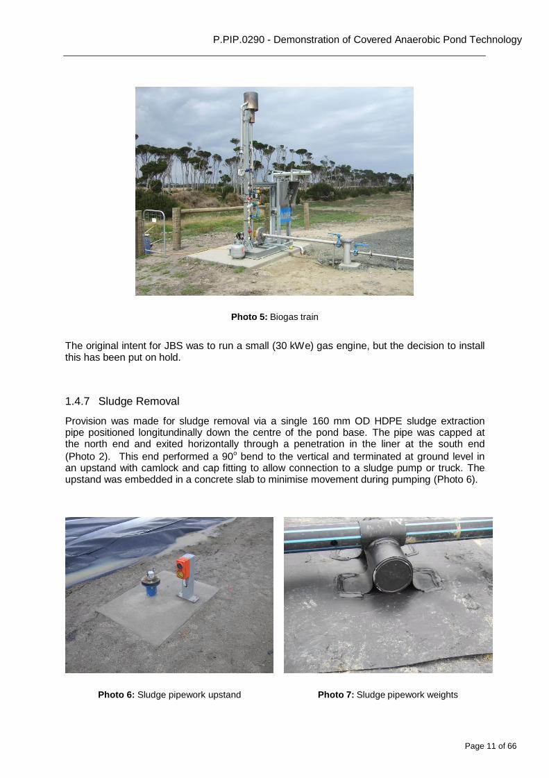
1.4.7 Sludge Removal
Provision was made for sludge removal via a single 160 mm OD HDPE sludge extraction pipe positioned longitundinally down the centre of the pond base. The pipe was capped at the north end and exited horizontally through a penetration in the liner at the south end
(Photo 2). This end performed a 90o bend to the vertical and terminated at ground level in an upstand with camlock and cap fitting to allow connection to a sludge pump or truck. The upstand was embedded in a concrete slab to minimise movement during pumping (Photo 6).
Photo 6: Sludge pipework upstand Photo 7: Sludge pipework weights

Page 12 of 66
P.PIP.0290 - Demonstration of Covered Anaerobic Pond Technology
The pipe was elevated approximately 200 mm off the CAL base by a series of 160 mm OD concrete-filled weights to minimise movement of the pipe and to negate its buoyancy if filled with biogas. The weights were capped water tight with HDPE caps to prevent concrete erosion in the slightly acidic conditions in the CAL (see Photo 7) and held in place by straps welded to a HDPE wear strip.
The pipe (24 m length on the pond base) was drilled with 16 x 30 mm diameter holes for sludge entry. The holes were on alternate sides of the pipe and positioned to avoid the weights. The hole spacings increased as the distance to the sludge discharge point reduced to avoid rat-holing as much as possible.
Page 13 of 66
P.PIP.0290 - Demonstration of Covered Anaerobic Pond Technology
2 Project objectives
The project goal was to demonstrate the operation of covered anaerobic pond technology to drive the uptake in Australian meat processing industry.
The project objectives were to:
Collect and analyse CAL data from a rigorous monitoring program over a 9 month
period. The data sought to capture two critical stages of CAL operation:
o Start-up phase. This can be reasonably lengthy, especially for greenfield sites. There are no publically available data regarding this period for meat processing ponds;
o Normal operation. Of special interest is the impact of the usual 5 day on/ 2
day off processing week on pond operation and biogas production and quality.
This data will help to reduce the uncertainties, risk and cost of installing methane recovery and use systems in the red meat processing industry.
Investigate sludge accumulation and crust build up over the investigation period.
Communicate the benefits of methane recovery and use as a clean energy source through final deliverables.
Page 14 of 66
P.PIP.0290 - Demonstration of Covered Anaerobic Pond Technology
Op
era
tio
n
ph
ase
Co
nst
ruct
ion
p
has
e
3 Methodology
3.1 CAL Start-up
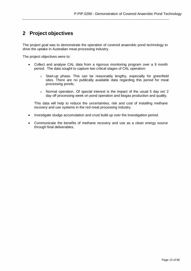
Figure 1 outlines the timing of the construction and operation phases of the project. There were extensive delays due to wet weather during excavation.
Cover installation is preferably conducted on a filled pond. For greenfield sites this is a challenge since the good quality water preferred for filling (such as treated effluent) is not readily available and potable water is expensive. At King Island the pond was initially filled in November 2011 with a mix of bore water and raw wastewater. No difficulties were experienced using this mix.
Commissioning was initiated by adding the full wastewater flow into the CAL on the 13th
December 2011. The entire wastewater flow continued to enter the CAL from this day onwards. No inoculum or sludge was added to assist startup due to the remoteness of the site and the absence of other suitable wastewater treatment systems on the island.
Excavation and lining
Filled with bore & raw wastewater
Installed cover and biogas train
CAL operational
Biogas flare operational
Figure 1: CAL start up time line
3.2 Wastewater Monitoring
Wastewater monitoring enabled the characterisation of the effluent flow and quality entering and leaving the CAL.
3.2.1 Wastewater Flow
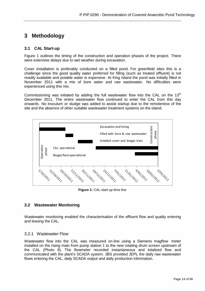
Wastewater flow into the CAL was measured on-line using a Siemens magflow meter installed on the rising main from pump station 1 to the new rotating drum screen upstream of the CAL (Photo 8). The flowmeter recorded instantaneous and totalized flow and communicated with the plant’s SCADA system. JBS provided JEPL the daily raw wastewater flows entering the CAL, daily SCADA output and daily production information.
Page 15 of 66
P.PIP.0290 - Demonstration of Covered Anaerobic Pond Technology
Rotary screen
CAL influent
Siemens magflow meter
Photo 8: Screening and instrumentation upstream of CAL
3.2.2 Wastewater Characterisation
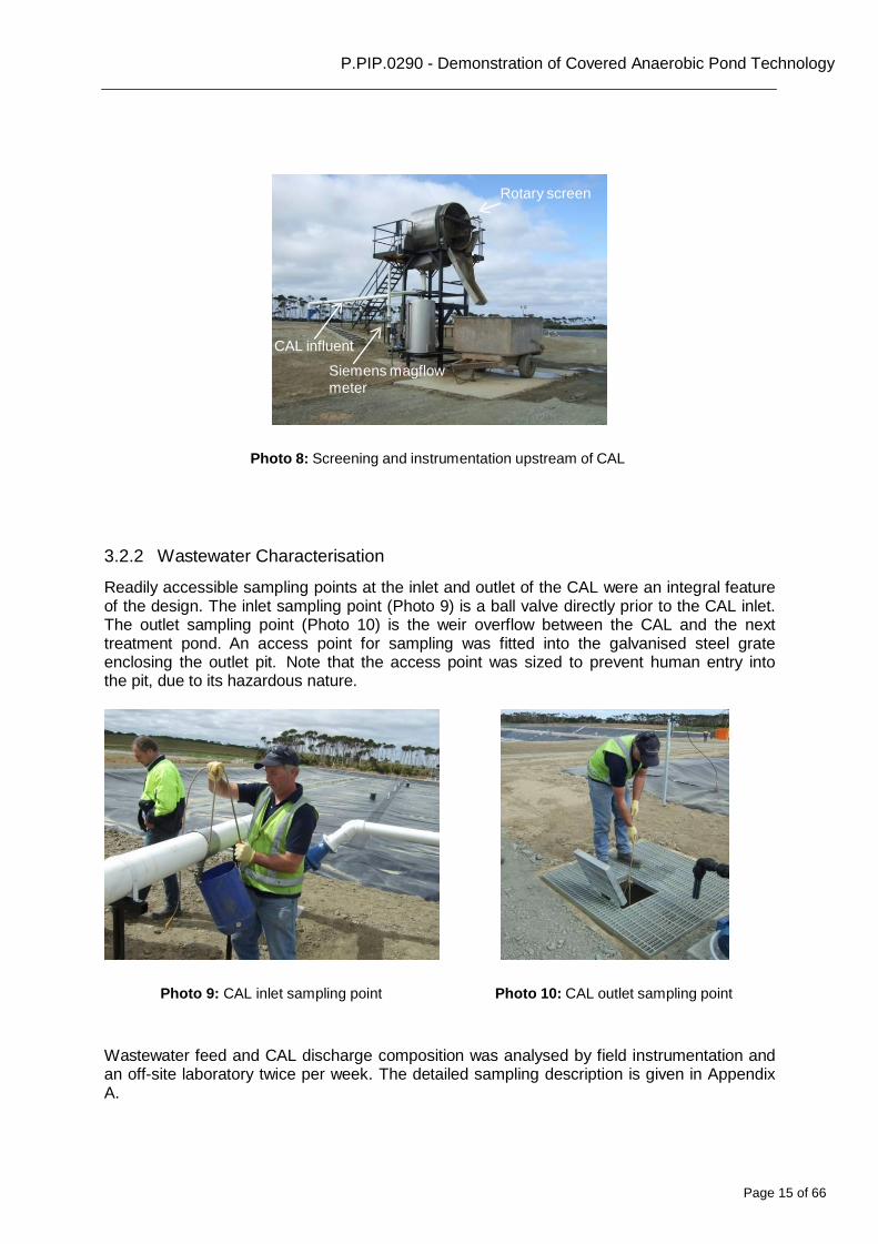
Readily accessible sampling points at the inlet and outlet of the CAL were an integral feature of the design. The inlet sampling point (Photo 9) is a ball valve directly prior to the CAL inlet. The outlet sampling point (Photo 10) is the weir overflow between the CAL and the next treatment pond. An access point for sampling was fitted into the galvanised steel grate enclosing the outlet pit. Note that the access point was sized to prevent human entry into the pit, due to its hazardous nature.
Photo 9: CAL inlet sampling point Photo 10: CAL outlet sampling point
Wastewater feed and CAL discharge composition was analysed by field instrumentation and an off-site laboratory twice per week. The detailed sampling description is given in Appendix A.
Page 16 of 66
P.PIP.0290 - Demonstration of Covered Anaerobic Pond Technology
1. Field measurements by King Island personnel recorded pH, temperature, and conductivity using a portable Hach HQ40d instrument supplied by JEPL. The visual appearance and odour of the effluent was also noted.
2. Laboratory analysis by EML (Chem) provided information on the following
parameters; pH, COD, BOD5, oil and grease, TSS, volatile fatty acids (VFA), total alkalinity (TA), ammonia and total kjeldahl nitrogen measured as TKN.
Raw effluent composition over a typical production day was investigated three times during the monitoring period. Raw effluent samples were collected over a typical production day and analysed by field instrumentation and laboratory analysis. The frequency and handling of each sampling regime are as follows:
1. 9th February 2012.
8 equal volume grab samples collected at approximately 1 hour intervals over production day and composited for laboratory analysis.
2. 4th June 2012. 6 equal volume grab samples collected at approximately 1 hour intervals from 11am to 4pm and composited for laboratory analysis.
3. 5th June 2012. a. 11 equal volume grab samples collected at 1 hour intervals from 7am to 5pm,
analysed for pH, temperature and conductivity using field instrumentation and composited for laboratory analysis.
b. 6 grab samples collected at 2 hour intervals from 7am to 5pm, analysed for pH, temperature and conductivity using field instrumentation and individual samples sent for laboratory analysis.
3.3 Biogas Monitoring
Online biogas monitoring of the methane composition, biogas flow and the pressure under the CAL cover was recorded to the sites SCADA system. An example of a SCADA output is shown in Appendix B. Further laboratory and field analysis of the biogas was performed by
The Odour Unit on 5th and 6th June 2012.
3.3.1 Biogas Flow
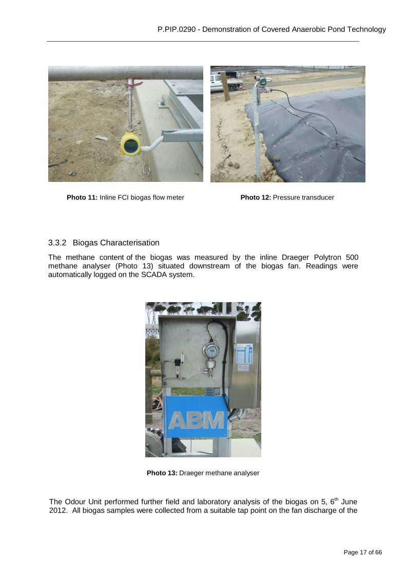
Instantaneous and cumulative biogas flow from an FCI ST51 in-line gas flow meter (Photo 11) was recorded each minute to the SCADA system. King Island personnel also collected this information and commented on the cover inflation and the colour of the flame during twice weekly sampling.
The biogas pressure under the CAL cover was measured by Yokogawa pressure transducer (Photo 12) and was logged on the SCADA system.
Page 17 of 66
P.PIP.0290 - Demonstration of Covered Anaerobic Pond Technology
Photo 11: Inline FCI biogas flow meter Photo 12: Pressure transducer
3.3.2 Biogas Characterisation
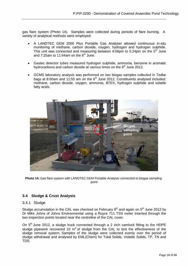
The methane content of the biogas was measured by the inline Draeger Polytron 500 methane analyser (Photo 13) situated downstream of the biogas fan. Readings were automatically logged on the SCADA system.
Photo 13: Draeger methane analyser
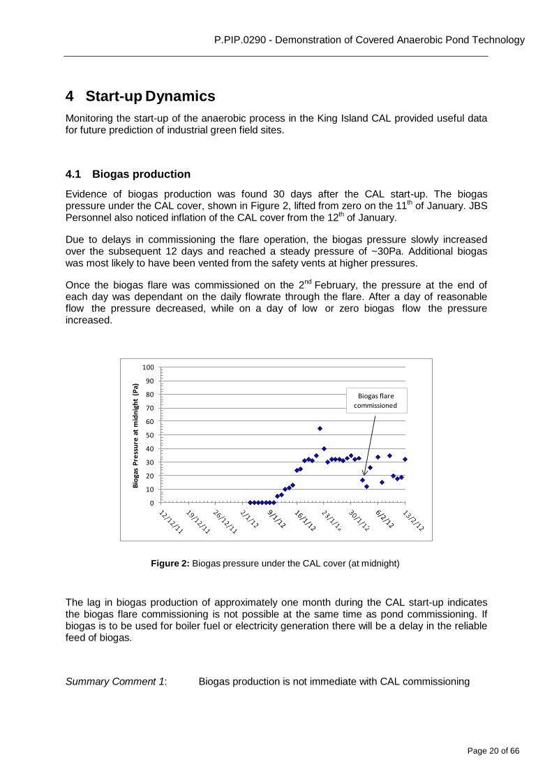
The Odour Unit performed further field and laboratory analysis of the biogas on 5, 6th June 2012. All biogas samples were collected from a suitable tap point on the fan discharge of the
Page 18 of 66
P.PIP.0290 - Demonstration of Covered Anaerobic Pond Technology
gas flare system (Photo 14). Samples were collected during periods of flare burning. A variety of analytical methods were employed:
A LANDTEC GEM 2000 Plus Portable Gas Analyser allowed continuous in-situ
monitoring of methane, carbon dioxide, oxygen, hydrogen and hydrogen sulphide.
This unit was connected and measuring between 4:06pm to 5:24pm on the 5th June
and 7:25am to 11:44am on the 6th June.
Gastec detector tubes measured hydrogen sulphide, ammonia, benzene in aromatic hydrocarbons and carbon dioxide at various times on the 6th June 2012.
GCMS laboratory analysis was performed on two biogas samples collected in Tedlar
bags at 8:00am and 11:55 am on the 6th June 2012. Constituents analysed included: methane, carbon dioxide, oxygen, ammonia, BTEX, hydrogen sulphide and volatile fatty acids.
Biogas
sampling point
Photo 14: Gas flare system with LANDTEC GEM Portable Analyser connected to biogas sampling
point
3.4 Sludge & Crust Analysis
3.4.1 Sludge
Sludge accumulation in the CAL was checked on February 9th and again on 5th June 2012 by Dr Mike Johns of Johns Environmental using a Royce 711 TSS meter inserted through the two inspection points located near the centreline of the CAL cover.
On 5th June 2012, a sludge truck connected through a 2 inch camlock fitting to the HDPE
sludge pipework recovered 10 m3 of sludge from the CAL to test the effectiveness of the sludge removal system. Samples of the sludge were collected evenly over the period of sludge withdrawal and analysed by EML(Chem) for Total Solids, Volatile Solids, TP, TN and TDS.

Page 19 of 66
P.PIP.0290 - Demonstration of Covered Anaerobic Pond Technology
3.4.2 Crust
Crust accumulation was assessed using the inspection ports on February 9th and again on 5th
June 2012. The assessment involved quantitative measurement of crust depth at the two
inspection ports. Crust samples were collected from each port on the 5th June and analysed by EML(Chem) for total Solids, Volatile Solids, TN, TP and Oil and Grease.
A physical assessment by walking on the cover was also conducted to determine if noticeable build up was occurring under the cover.
Page 20 of 66
P.PIP.0290 - Demonstration of Covered Anaerobic Pond Technology
Bio
gas
Pre
ssu
re a
t m
idn
igh
t (P
a)
4 Start-up Dynamics
Monitoring the start-up of the anaerobic process in the King Island CAL provided useful data for future prediction of industrial green field sites.
4.1 Biogas production
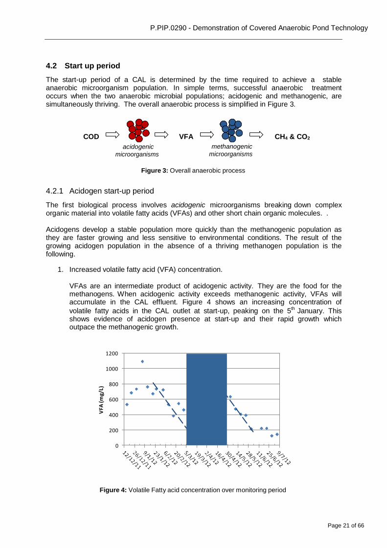
Evidence of biogas production was found 30 days after the CAL start-up. The biogas pressure under the CAL cover, shown in Figure 2, lifted from zero on the 11th of January. JBS Personnel also noticed inflation of the CAL cover from the 12th of January.
Due to delays in commissioning the flare operation, the biogas pressure slowly increased over the subsequent 12 days and reached a steady pressure of ~30Pa. Additional biogas was most likely to have been vented from the safety vents at higher pressures.
Once the biogas flare was commissioned on the 2nd February, the pressure at the end of each day was dependant on the daily flowrate through the flare. After a day of reasonable flow the pressure decreased, while on a day of low or zero biogas flow the pressure increased.
100
90
80
70
60
50
40
30
20
10
0
Biogas flare
commissioned
Figure 2: Biogas pressure under the CAL cover (at midnight)
The lag in biogas production of approximately one month during the CAL start-up indicates the biogas flare commissioning is not possible at the same time as pond commissioning. If biogas is to be used for boiler fuel or electricity generation there will be a delay in the reliable feed of biogas.
Summary Comment 1: Biogas production is not immediate with CAL commissioning
Page 21 of 66
P.PIP.0290 - Demonstration of Covered Anaerobic Pond Technology
VFA
(mg/
L)
4.2 Start up period
The start-up period of a CAL is determined by the time required to achieve a stable anaerobic microorganism population. In simple terms, successful anaerobic treatment occurs when the two anaerobic microbial populations; acidogenic and methanogenic, are simultaneously thriving. The overall anaerobic process is simplified in Figure 3.
COD VFA CH4 & CO2
acidogenic microorganisms
methanogenic microorganisms
Figure 3: Overall anaerobic process
4.2.1 Acidogen start-up period
The first biological process involves acidogenic microorganisms breaking down complex organic material into volatile fatty acids (VFAs) and other short chain organic molecules. .
Acidogens develop a stable population more quickly than the methanogenic population as they are faster growing and less sensitive to environmental conditions. The result of the growing acidogen population in the absence of a thriving methanogen population is the following.
1. Increased volatile fatty acid (VFA) concentration.
VFAs are an intermediate product of acidogenic activity. They are the food for the methanogens. When acidogenic activity exceeds methanogenic activity, VFAs will accumulate in the CAL effluent. Figure 4 shows an increasing concentration of
volatile fatty acids in the CAL outlet at start-up, peaking on the 5th January. This shows evidence of acidogen presence at start-up and their rapid growth which outpace the methanogenic growth.
1200
1000
800
600
400
200
0
Figure 4: Volatile Fatty acid concentration over monitoring period
Page 22 of 66
P.PIP.0290 - Demonstration of Covered Anaerobic Pond Technology
NH
3 (
mg/
L)
TKN
(m
g/L)
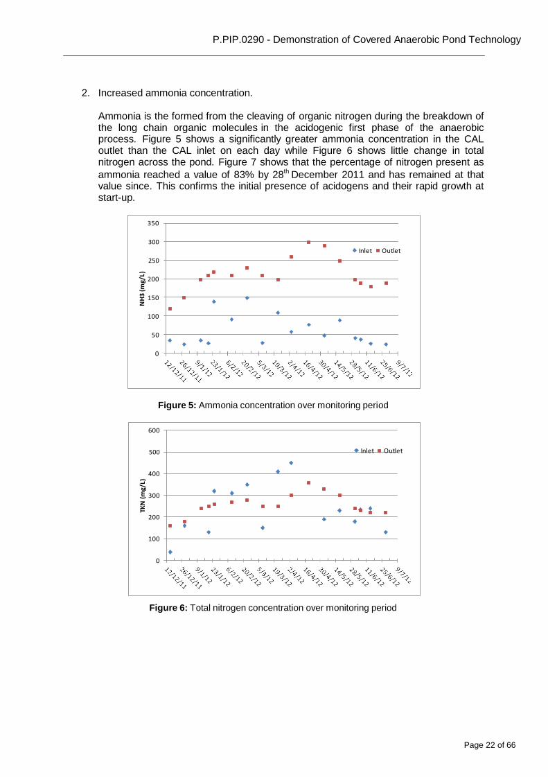
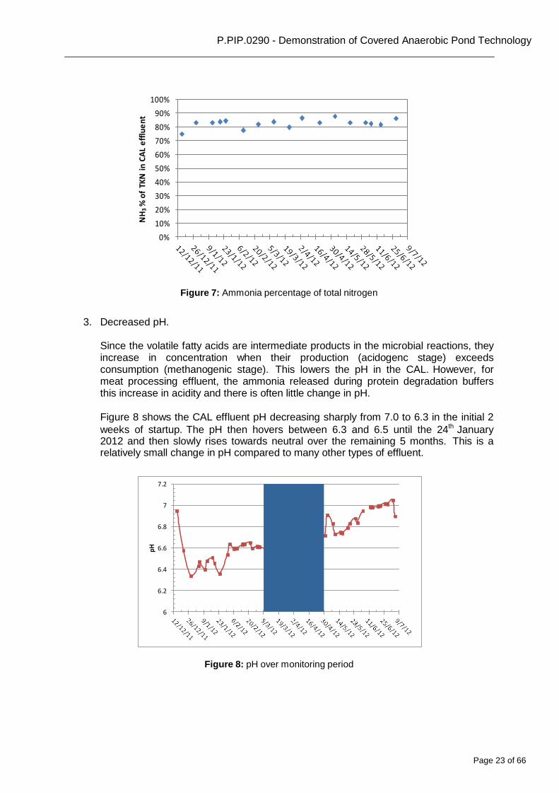
2. Increased ammonia concentration.
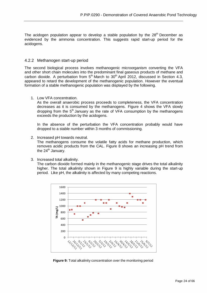
Ammonia is the formed from the cleaving of organic nitrogen during the breakdown of the long chain organic molecules in the acidogenic first phase of the anaerobic process. Figure 5 shows a significantly greater ammonia concentration in the CAL outlet than the CAL inlet on each day while Figure 6 shows little change in total nitrogen across the pond. Figure 7 shows that the percentage of nitrogen present as
ammonia reached a value of 83% by 28th December 2011 and has remained at that value since. This confirms the initial presence of acidogens and their rapid growth at start-up.
350
300
250
Inlet Outlet
200
150
100
50
0
Figure 5: Ammonia concentration over monitoring period
600
500 Inlet Outlet
400
300
200
100
0
Figure 6: Total nitrogen concentration over monitoring period
Page 23 of 66
P.PIP.0290 - Demonstration of Covered Anaerobic Pond Technology
NH
3 %
of
TKN
in
CA
L e
fflu
en
t p
H
100%
90%
80%
70%
60%
50%
40%
30%
20%
10%
0%
Figure 7: Ammonia percentage of total nitrogen
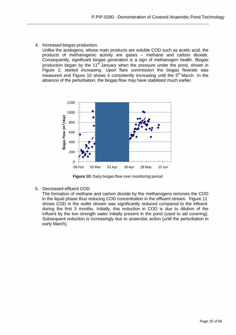
3. Decreased pH.
Since the volatile fatty acids are intermediate products in the microbial reactions, they increase in concentration when their production (acidogenc stage) exceeds consumption (methanogenic stage). This lowers the pH in the CAL. However, for meat processing effluent, the ammonia released during protein degradation buffers this increase in acidity and there is often little change in pH.
Figure 8 shows the CAL effluent pH decreasing sharply from 7.0 to 6.3 in the initial 2
weeks of startup. The pH then hovers between 6.3 and 6.5 until the 24th January 2012 and then slowly rises towards neutral over the remaining 5 months. This is a relatively small change in pH compared to many other types of effluent.
7.2
7
6.8
6.6
6.4
6.2
6
Figure 8: pH over monitoring period
Page 24 of 66
P.PIP.0290 - Demonstration of Covered Anaerobic Pond Technology
TA (
mg/
L)
The acidogen population appear to develop a stable population by the 28th December as evidenced by the ammonia concentration. This suggests rapid start-up period for the acidogens.
4.2.2 Methanogen start-up period
The second biological process involves methanogenic microorganism converting the VFA and other short chain molecules into the predominant final gaseous products of methane and
carbon dioxide. A perturbation from 5th March to 30th April 2012, discussed in Section 4.3, appeared to retard the development of the methanogenic population. However the eventual formation of a stable methanogenic population was displayed by the following.
1. Low VFA concentration.
As the overall anaerobic process proceeds to completeness, the VFA concentration decreases as it is consumed by the methanogens. Figure 4 shows the VFA slowly
dropping from the 5th January as the rate of VFA consumption by the methanogens exceeds the production by the acidogens.
In the absence of the perturbation the VFA concentration probably would have dropped to a stable number within 3 months of commissioning.
2. Increased pH towards neutral.
The methanogens consume the volatile fatty acids for methane production, which removes acidic products from the CAL. Figure 8 shows an increasing pH trend from
the 24th January.
3. Increased total alkalinity. The carbon dioxide formed mainly in the methanogenic stage drives the total alkalinity higher. The total alkalinity shown in Figure 9 is highly variable during the start-up period. Like pH, the alkalinity is affected by many competing reactions.
1600
1400
1200
1000
800
600
400
200
0
Figure 9: Total alkalinity concentration over the monitoring period
Page 25 of 66
P.PIP.0290 - Demonstration of Covered Anaerobic Pond Technology
n w o td u h s
Bio
gas
Flo
w (
m3/d
ay)
4. Increased biogas production. Unlike the acidogens, whose main products are soluble COD such as acetic acid, the products of methanogenic activity are gases – methane and carbon dioxide. Consequently, significant biogas generation is a sign of methanogen health. Biogas
production began by the 11th January when the pressure under the pond, shown in Figure 2, started increasing. Upon flare commission the biogas flowrate was
measured and Figure 10 shows it consistently increasing until the 5th March. In the absence of the perturbation, the biogas flow may have stabilised much earlier.
1200
1000
800
600
400
200
0
06 Feb 05 Mar 02 Apr 30 Apr 28 May 25 Jun
Figure 10: Daily biogas flow over monitoring period
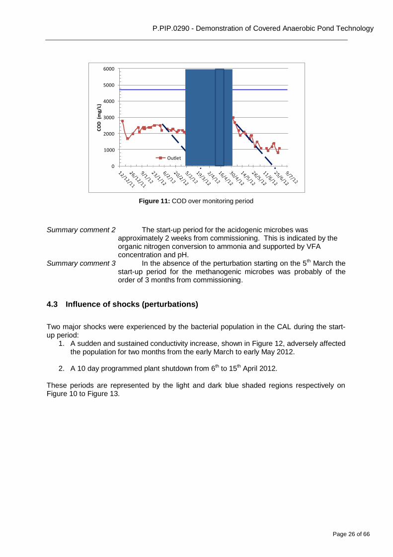
5. Decreased effluent COD The formation of methane and carbon dioxide by the methanogens removes the COD in the liquid phase thus reducing COD concentration in the effluent stream. Figure 11 shows COD in the outlet stream was significantly reduced compared to the influent during the first 3 months. Initially, this reduction in COD is due to dilution of the influent by the low strength water initially present in the pond (used to aid covering). Subsequent reduction is increasingly due to anaerobic action (until the perturbation in early March).
Page 26 of 66
P.PIP.0290 - Demonstration of Covered Anaerobic Pond Technology
Composite Inlet
CO
D (
mg/
L)
6000
5000
4000
3000
2000
1000
0
Outlet
Figure 11: COD over monitoring period
Summary comment 2 The start-up period for the acidogenic microbes was approximately 2 weeks from commissioning. This is indicated by the organic nitrogen conversion to ammonia and supported by VFA concentration and pH.
Summary comment 3 In the absence of the perturbation starting on the 5th March the start-up period for the methanogenic microbes was probably of the order of 3 months from commissioning.
4.3 Influence of shocks (perturbations)
Two major shocks were experienced by the bacterial population in the CAL during the start- up period:
1. A sudden and sustained conductivity increase, shown in Figure 12, adversely affected the population for two months from the early March to early May 2012.
2. A 10 day programmed plant shutdown from 6th to 15th April 2012.
These periods are represented by the light and dark blue shaded regions respectively on Figure 10 to Figure 13.
Page 27 of 66
P.PIP.0290 - Demonstration of Covered Anaerobic Pond Technology
VFA
(mg/
L)
Co
nd
uct
ivit
y O
ut
(S/
cm)
11,000
10,000
9,000
8,000
7,000
6,000
5,000
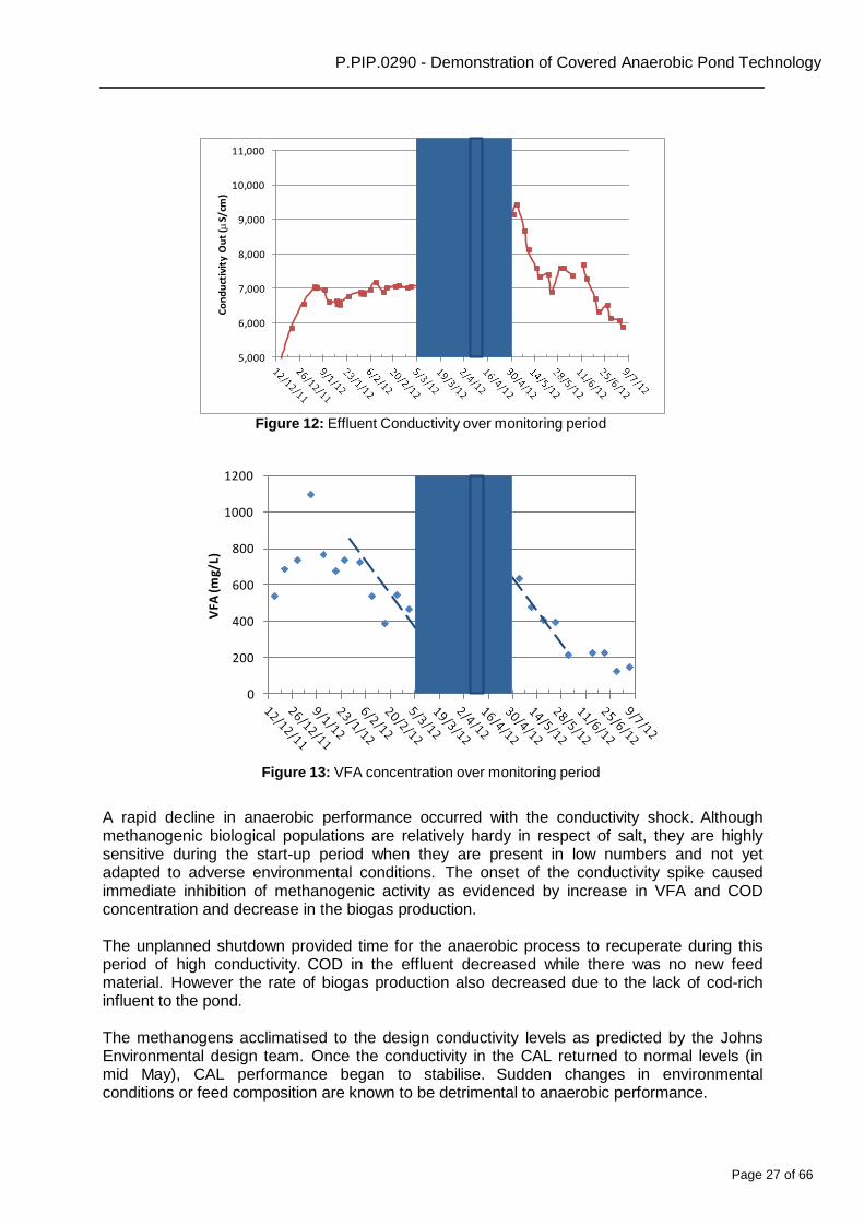
Figure 12: Effluent Conductivity over monitoring period
1200
1000
800
600
400
200
0
Figure 13: VFA concentration over monitoring period
A rapid decline in anaerobic performance occurred with the conductivity shock. Although methanogenic biological populations are relatively hardy in respect of salt, they are highly sensitive during the start-up period when they are present in low numbers and not yet adapted to adverse environmental conditions. The onset of the conductivity spike caused immediate inhibition of methanogenic activity as evidenced by increase in VFA and COD concentration and decrease in the biogas production.
The unplanned shutdown provided time for the anaerobic process to recuperate during this period of high conductivity. COD in the effluent decreased while there was no new feed material. However the rate of biogas production also decreased due to the lack of cod-rich influent to the pond.
The methanogens acclimatised to the design conductivity levels as predicted by the Johns Environmental design team. Once the conductivity in the CAL returned to normal levels (in mid May), CAL performance began to stabilise. Sudden changes in environmental conditions or feed composition are known to be detrimental to anaerobic performance.
Page 28 of 66
P.PIP.0290 - Demonstration of Covered Anaerobic Pond Technology
VFA
/ T
A
Summary comment 4 Anaerobic processes are highly sensitive to rapid changes in the CAL environment or feed composition during start-up.
4.4 Microbial Stress Indicators
Stress to the methanogens causes decreased anaerobic performance. Common stressors are start-up, changing or adverse environmental conditions and shock loads in the feed. An indication of CAL health is useful to allow mitigation before complete failure occurs. Traditionally, pH measurement is used for this purpose. Unfortunately, this is unreliable for protein-rich wastewater.
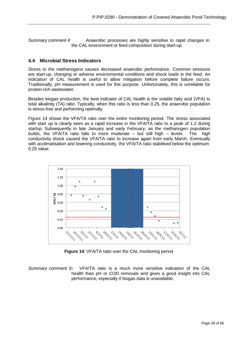
Besides biogas production, the best indicator of CAL health is the volatile fatty acid (VFA) to total alkalinity (TA) ratio. Typically, when this ratio is less than 0.25, the anaerobic population is stress-free and performing optimally.
Figure 14 shows the VFA/TA ratio over the entire monitoring period. The stress associated with start up is clearly seen as a rapid increase in the VFA/TA ratio to a peak of 1.2 during startup. Subsequently in late January and early February, as the methanogen population builds, the VFA/TA ratio falls to more moderate – but still high – levels. The high conductivity shock caused the VFA/TA ratio to increase again from early March. Eventually with acclimatisation and lowering conductivity, the VFA/TA ratio stabilised below the optimum 0.25 value.
1.40
1.20
1.00
0.80
0.60
0.40
0.20
0.00
Figure 14: VFA/TA ratio over the CAL monitoring period
Summary comment 5: VFA/TA ratio is a much more sensitive indication of the CAL health than pH or COD removals and gives a good insight into CAL performance, especially if biogas data is unavailable.
Page 29 of 66
P.PIP.0290 - Demonstration of Covered Anaerobic Pond Technology
Tem
pe
ratu
re (C
)
4.5 Pond Temperature
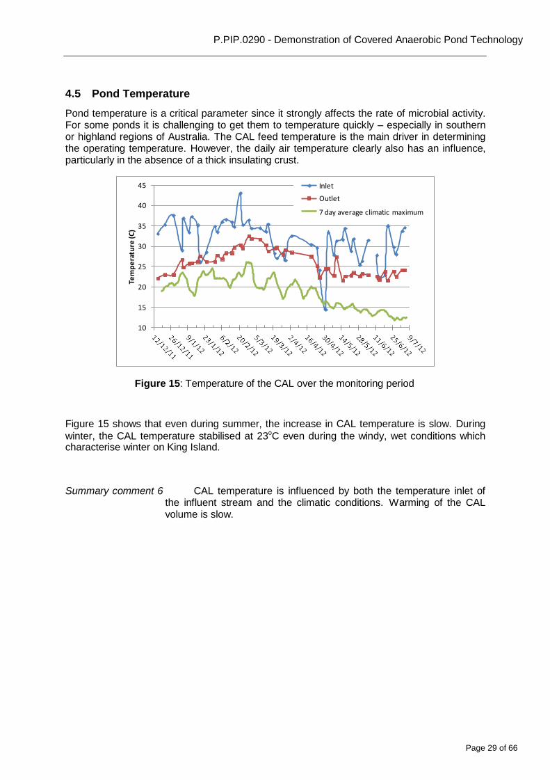
Pond temperature is a critical parameter since it strongly affects the rate of microbial activity. For some ponds it is challenging to get them to temperature quickly – especially in southern or highland regions of Australia. The CAL feed temperature is the main driver in determining the operating temperature. However, the daily air temperature clearly also has an influence, particularly in the absence of a thick insulating crust.
45 Inlet
Outlet 40
7 day average climatic maximum
35
30
25
20
15
10
Figure 15: Temperature of the CAL over the monitoring period
Figure 15 shows that even during summer, the increase in CAL temperature is slow. During
winter, the CAL temperature stabilised at 23oC even during the windy, wet conditions which characterise winter on King Island.
Summary comment 6 CAL temperature is influenced by both the temperature inlet of
the influent stream and the climatic conditions. Warming of the CAL volume is slow.
Page 30 of 66
P.PIP.0290 - Demonstration of Covered Anaerobic Pond Technology
Bio
gas
Flo
w (
m3/d
ay)
shu
tdo
wn
5 Normal Operating Performance
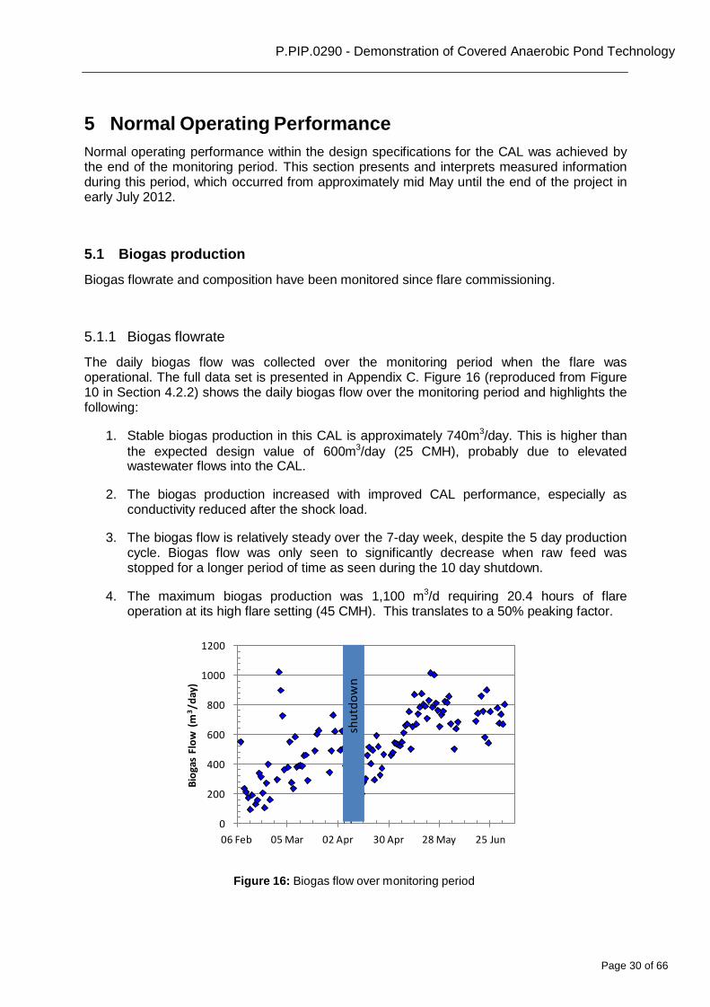
Normal operating performance within the design specifications for the CAL was achieved by the end of the monitoring period. This section presents and interprets measured information during this period, which occurred from approximately mid May until the end of the project in early July 2012.
5.1 Biogas production
Biogas flowrate and composition have been monitored since flare commissioning.
5.1.1 Biogas flowrate
The daily biogas flow was collected over the monitoring period when the flare was operational. The full data set is presented in Appendix C. Figure 16 (reproduced from Figure 10 in Section 4.2.2) shows the daily biogas flow over the monitoring period and highlights the following:
1. Stable biogas production in this CAL is approximately 740m3/day. This is higher than
the expected design value of 600m3/day (25 CMH), probably due to elevated wastewater flows into the CAL.
2. The biogas production increased with improved CAL performance, especially as
conductivity reduced after the shock load.
3. The biogas flow is relatively steady over the 7-day week, despite the 5 day production cycle. Biogas flow was only seen to significantly decrease when raw feed was stopped for a longer period of time as seen during the 10 day shutdown.
4. The maximum biogas production was 1,100 m3/d requiring 20.4 hours of flare operation at its high flare setting (45 CMH). This translates to a 50% peaking factor.
1200
1000
800
600
400
200
0
06 Feb 05 Mar 02 Apr 30 Apr 28 May 25 Jun
Figure 16: Biogas flow over monitoring period
Page 31 of 66
P.PIP.0290 - Demonstration of Covered Anaerobic Pond Technology
nn ww oo tdtd uu hh ss
Bio
gas
Me
than
e %
Summary comment 7: Biogas flowrate increases during start-up and is affected by adverse conditions in the pond.
Summary comment 8: The maximum gas production observed is 1,100 m3/d
representing a peaking factor of 50%.
Summary comment 9: Biogas production is relatively constant during the week,
despite the 5 day operating profile.
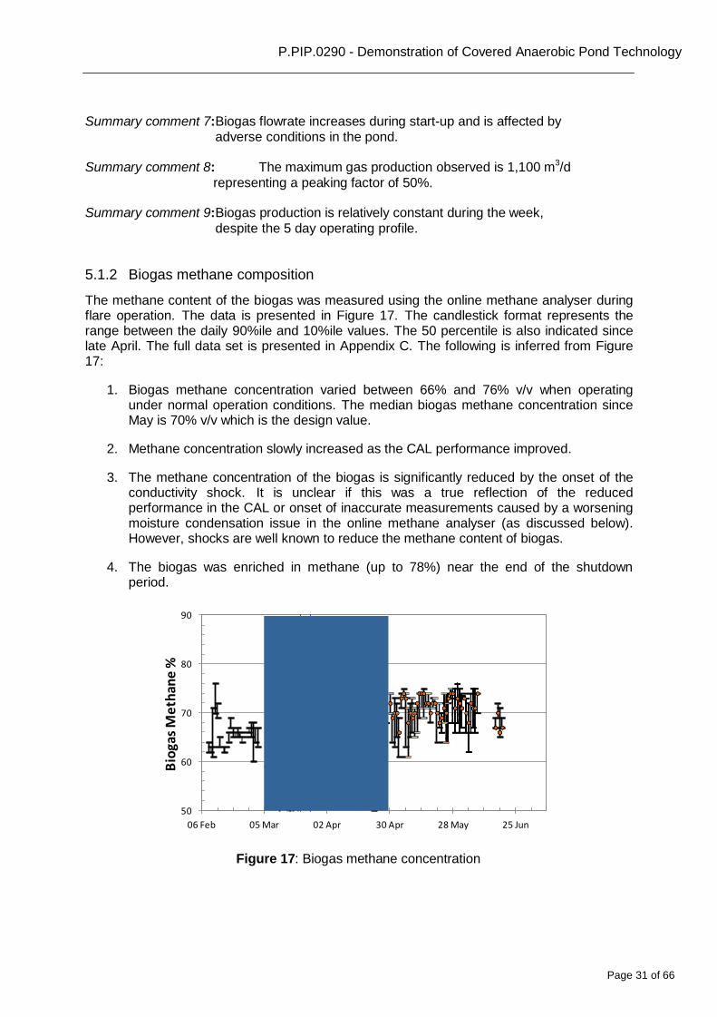
5.1.2 Biogas methane composition
The methane content of the biogas was measured using the online methane analyser during flare operation. The data is presented in Figure 17. The candlestick format represents the range between the daily 90%ile and 10%ile values. The 50 percentile is also indicated since late April. The full data set is presented in Appendix C. The following is inferred from Figure 17:
1. Biogas methane concentration varied between 66% and 76% v/v when operating
under normal operation conditions. The median biogas methane concentration since May is 70% v/v which is the design value.
2. Methane concentration slowly increased as the CAL performance improved.
3. The methane concentration of the biogas is significantly reduced by the onset of the
conductivity shock. It is unclear if this was a true reflection of the reduced performance in the CAL or onset of inaccurate measurements caused by a worsening moisture condensation issue in the online methane analyser (as discussed below). However, shocks are well known to reduce the methane content of biogas.
4. The biogas was enriched in methane (up to 78%) near the end of the shutdown
period.
90
80
70
60
50
06 Feb 05 Mar 02 Apr 30 Apr 28 May 25 Jun
Figure 17: Biogas methane concentration
Page 32 of 66
P.PIP.0290 - Demonstration of Covered Anaerobic Pond Technology
Me
than
e c
on
cen
trat
ion
dif
fere
nce
-
Po
rtab
le A
nal
yse
r -
On
line
An
alys
er
CH
4 %
v/v
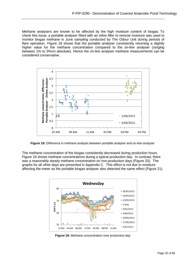
Methane analysers are known to be affected by the high moisture content of biogas. To check this issue, a portable analyser fitted with an inline filter to remove moisture was used to monitor biogas methane in June sampling conducted by The Odour Unit during periods of flare operation. Figure 18 shows that the portable analyser consistently returning a slightly higher value for the methane concentration compared to the on-line analyser (ranging between 1% to 3%v/v absolute). Hence the on-line analyser methane measurements can be considered conservative.
4
3.5
3
2.5
2
1.5
1
0.5
0
5/06/2012
6/06/2012
07 AM 09 AM 11 AM 01 PM 03 PM 05 PM
Figure 18: Difference in methane analysis between portable analyser and on-line analyser
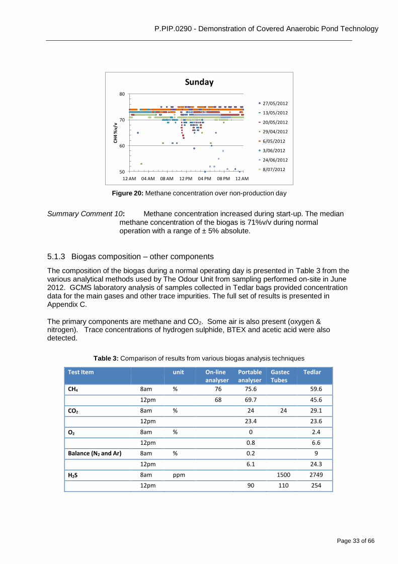
The methane concentration of the biogas consistently decreased during production hours. Figure 19 shows methane concentrations during a typical production day. In contrast, there was a reasonably steady methane concentration on non-production days (Figure 20). The graphs for all other days are presented in Appendix C. This effect is not due to moisture affecting the meter as the portable biogas analyser also detected the same effect (Figure 21).
Wednesday 80
70
60
50
30/05/2012
16/05/2012
23/05/2012
2-May
9/05/2012
6/06/2012
20/06/2012
27/06/2012
12 AM 04 AM 08 AM 12 PM 04 PM 08 PM 12 AM 4/07/2012
Figure 19: Methane concentration over production day
Page 33 of 66
P.PIP.0290 - Demonstration of Covered Anaerobic Pond Technology
CH
4 %
v/v
Sunday
80
70
60
50
27/05/2012
13/05/2012
20/05/2012
29/04/2012
6/05/2012
3/06/2012
24/06/2012
8/07/2012
12 AM 04 AM 08 AM 12 PM 04 PM 08 PM 12 AM
Figure 20: Methane concentration over non-production day
Summary Comment 10: Methane concentration increased during start-up. The median methane concentration of the biogas is 71%v/v during normal operation with a range of ± 5% absolute.
5.1.3 Biogas composition – other components
The composition of the biogas during a normal operating day is presented in Table 3 from the various analytical methods used by The Odour Unit from sampling performed on-site in June 2012. GCMS laboratory analysis of samples collected in Tedlar bags provided concentration data for the main gases and other trace impurities. The full set of results is presented in Appendix C.
The primary components are methane and CO2. Some air is also present (oxygen & nitrogen). Trace concentrations of hydrogen sulphide, BTEX and acetic acid were also detected.
Table 3: Comparison of results from various biogas analysis techniques
Test Item unit On-line analyser
Portable analyser
Gastec Tubes
Tedlar
CH4 8am % 76 75.6 59.6
12pm 68 69.7 45.6
CO2 8am % 24 24 29.1
12pm 23.4 23.6
O2 8am % 0 2.4
12pm 0.8 6.6
Balance (N2 and Ar) 8am % 0.2 9
12pm 6.1 24.3
H2S 8am ppm 1500 2749
12pm 90 110 254
Page 34 of 66
P.PIP.0290 - Demonstration of Covered Anaerobic Pond Technology
O2
(v
/v%
) C
O2
(v/
v%)
N2
& A
r (
v/v%
) C
H4
(v/
v%)
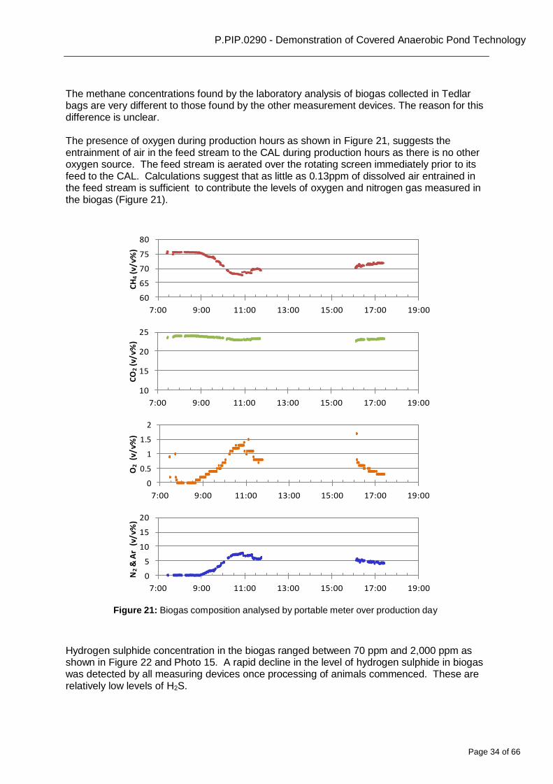
The methane concentrations found by the laboratory analysis of biogas collected in Tedlar bags are very different to those found by the other measurement devices. The reason for this difference is unclear.
The presence of oxygen during production hours as shown in Figure 21, suggests the entrainment of air in the feed stream to the CAL during production hours as there is no other oxygen source. The feed stream is aerated over the rotating screen immediately prior to its feed to the CAL. Calculations suggest that as little as 0.13ppm of dissolved air entrained in the feed stream is sufficient to contribute the levels of oxygen and nitrogen gas measured in the biogas (Figure 21).
80
75
70
65
60
7:00 9:00 11:00 13:00 15:00 17:00 19:00
25
20
15
10
7:00 9:00 11:00 13:00 15:00 17:00 19:00
2
1.5
1
0.5
0
7:00 9:00 11:00 13:00 15:00 17:00 19:00
20
15
10
5
0
7:00 9:00 11:00 13:00 15:00 17:00 19:00
Figure 21: Biogas composition analysed by portable meter over production day
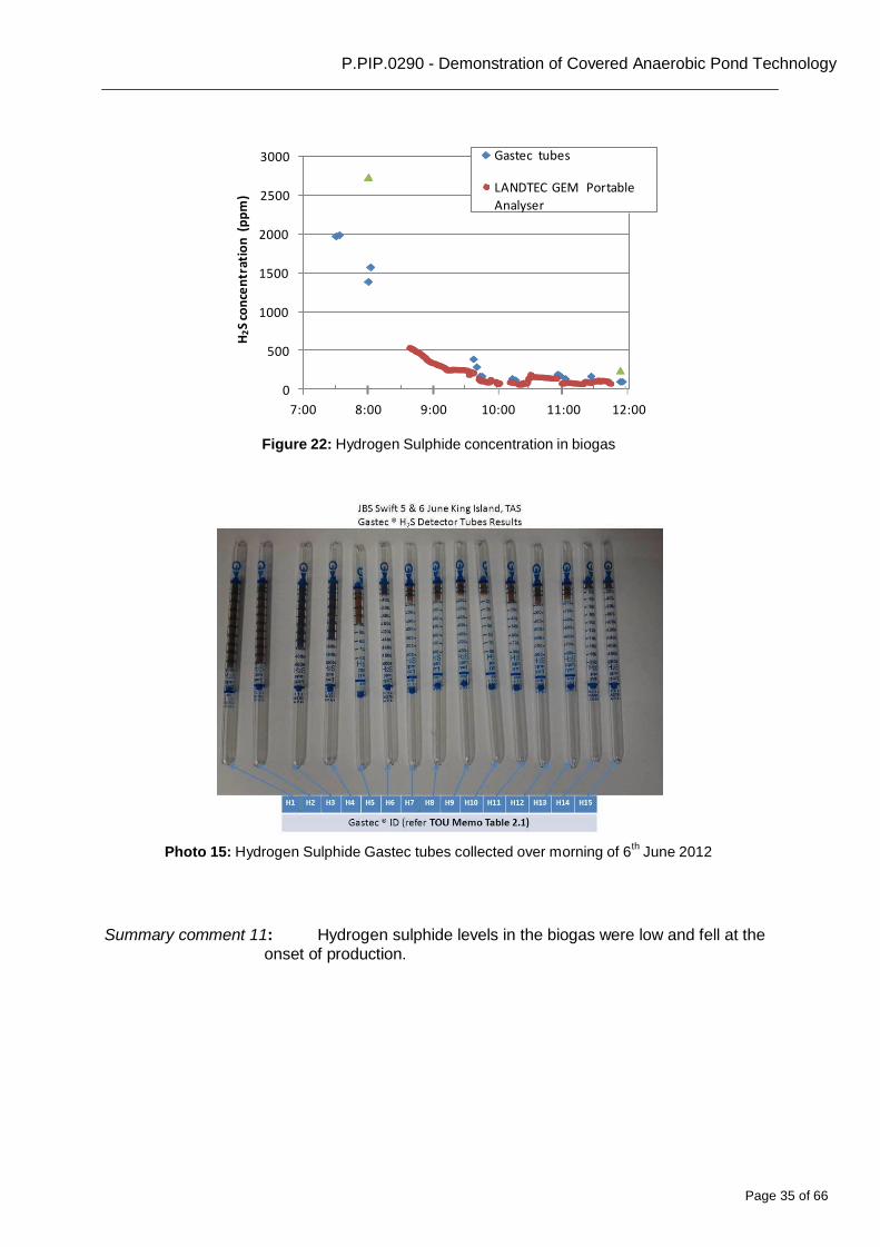
Hydrogen sulphide concentration in the biogas ranged between 70 ppm and 2,000 ppm as shown in Figure 22 and Photo 15. A rapid decline in the level of hydrogen sulphide in biogas was detected by all measuring devices once processing of animals commenced. These are relatively low levels of H2S.
Page 35 of 66
P.PIP.0290 - Demonstration of Covered Anaerobic Pond Technology
H2S
con
cen
trat
ion
(p
pm
)
3000
2500
Gastec tubes
LANDTEC GEM Portable
Analyser
2000
1500
1000
500
0
7:00 8:00 9:00 10:00 11:00 12:00
Figure 22: Hydrogen Sulphide concentration in biogas
Photo 15: Hydrogen Sulphide Gastec tubes collected over morning of 6th
June 2012
Summary comment 11: Hydrogen sulphide levels in the biogas were low and fell at the
onset of production.
Page 36 of 66
P.PIP.0290 - Demonstration of Covered Anaerobic Pond Technology
pH
Te
mp
era
ture
(C
)
Co
nd
uct
ivit
y (
mS/
cm)
5.2 Contaminant Removal from the Wastewater
5.2.1 Influent Composition
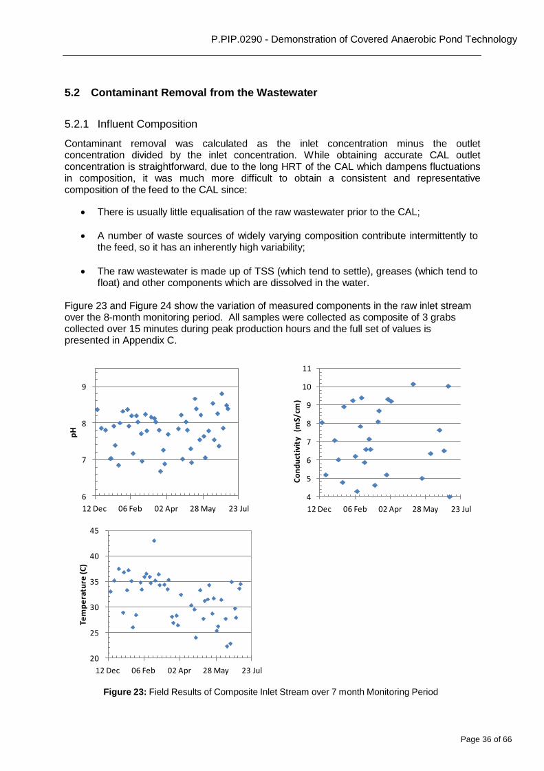
Contaminant removal was calculated as the inlet concentration minus the outlet concentration divided by the inlet concentration. While obtaining accurate CAL outlet concentration is straightforward, due to the long HRT of the CAL which dampens fluctuations in composition, it was much more difficult to obtain a consistent and representative composition of the feed to the CAL since:
There is usually little equalisation of the raw wastewater prior to the CAL;
A number of waste sources of widely varying composition contribute intermittently to the feed, so it has an inherently high variability;
The raw wastewater is made up of TSS (which tend to settle), greases (which tend to
float) and other components which are dissolved in the water.
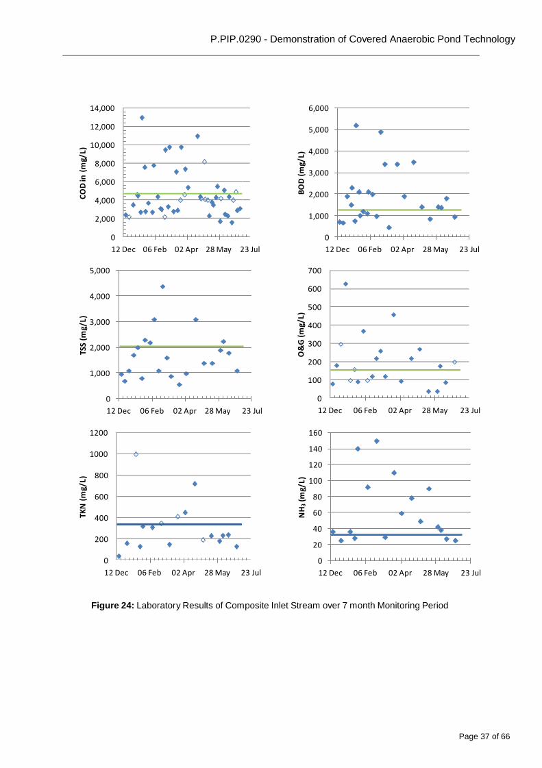
Figure 23 and Figure 24 show the variation of measured components in the raw inlet stream over the 8-month monitoring period. All samples were collected as composite of 3 grabs collected over 15 minutes during peak production hours and the full set of values is presented in Appendix C.
11
9 10
9
8 8
7
7 6
6
12 Dec 06 Feb 02 Apr 28 May 23 Jul
5
4
12 Dec 06 Feb 02 Apr 28 May 23 Jul
45
40
35
30
25
20
12 Dec 06 Feb 02 Apr 28 May 23 Jul
Figure 23: Field Results of Composite Inlet Stream over 7 month Monitoring Period
Page 37 of 66
P.PIP.0290 - Demonstration of Covered Anaerobic Pond Technology
TKN
(m
g/L)
TS
S (m
g/L)
C
OD
in (
mg/
L)
O&
G (
mg/
L)
NH
3 (
mg/
L)
BO
D (
mg/
L)
14,000
12,000
10,000
8,000
6,000
4,000
2,000
6,000
5,000
4,000
3,000
2,000
1,000
0
12 Dec 06 Feb 02 Apr 28 May 23 Jul
0
12 Dec 06 Feb 02 Apr 28 May 23 Jul
5,000 700
4,000
3,000
2,000
1,000
600
500
400
300
200
100
0
12 Dec 06 Feb 02 Apr 28 May 23 Jul
0
12 Dec 06 Feb 02 Apr 28 May 23 Jul
1200
1000
800
600
400
200
0
12 Dec 06 Feb 02 Apr 28 May 23 Jul
160
140
120
100
80
60
40
20
0
12 Dec 06 Feb 02 Apr 28 May 23 Jul
Figure 24: Laboratory Results of Composite Inlet Stream over 7 month Monitoring Period
Page 38 of 66
P.PIP.0290 - Demonstration of Covered Anaerobic Pond Technology
C
on
cen
trat
ion
(m
g/L)
C
on
cen
trat
ion
(mg/
L)
C
on
cen
trat
ion
(mg/
L)
Te
mp
era
ture
(C)
p
H
C
on
du
ctiv
ity
(mS/
cm)
6000 TSS 300
5000 COD 250
4000 200
Flo
w (
kL/h
)
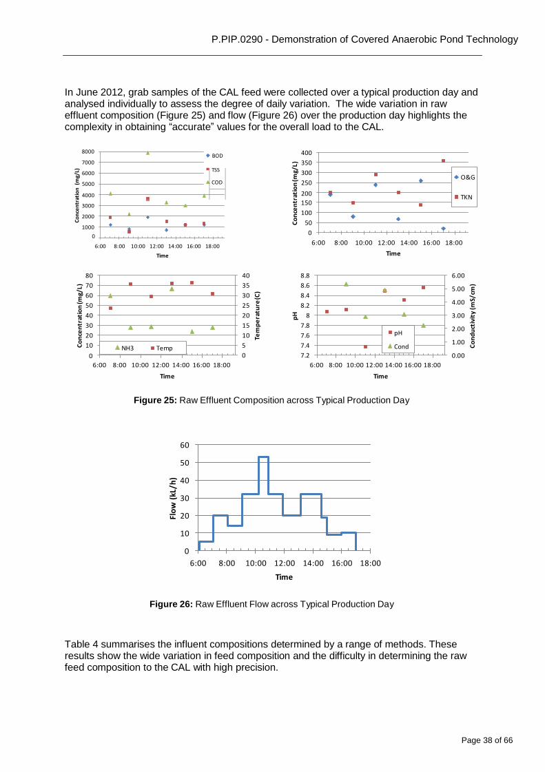
In June 2012, grab samples of the CAL feed were collected over a typical production day and analysed individually to assess the degree of daily variation. The wide variation in raw effluent composition (Figure 25) and flow (Figure 26) over the production day highlights the complexity in obtaining “accurate” values for the overall load to the CAL.
8000
7000
3000
2000
1000
0
BOD 400
350
150
100
50
0
O&G
TKN
6:00 8:00 10:00 12:00 14:00 16:00 18:00
Time
6:00 8:00 10:00 12:00 14:00 16:00 18:00
Time
80
70
60
50
40
30
20
10 NH3 Temp 0
40 8.8
35 8.6
30 8.4
25 8.2
20 8
15 7.8
10 7.6
5 7.4
0 7.2
pH
Cond
6.00
5.00
4.00
3.00
2.00
1.00
0.00
6:00 8:00 10:00 12:00 14:00 16:00 18:00
Time
6:00 8:00 10:00 12:00 14:00 16:00 18:00
Time
Figure 25: Raw Effluent Composition across Typical Production Day
60
50
40
30
20
10
0
6:00 8:00 10:00 12:00 14:00 16:00 18:00
Time
Figure 26: Raw Effluent Flow across Typical Production Day
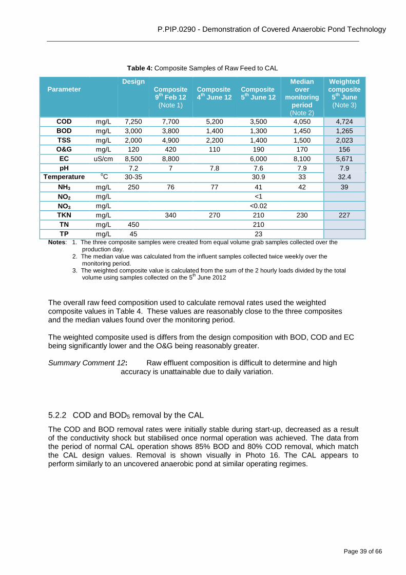
Table 4 summarises the influent compositions determined by a range of methods. These results show the wide variation in feed composition and the difficulty in determining the raw feed composition to the CAL with high precision.
Page 39 of 66
P.PIP.0290 - Demonstration of Covered Anaerobic Pond Technology
Table 4: Composite Samples of Raw Feed to CAL
Parameter
Design Composite 9
th Feb 12
(Note 1)
Composite 4
th June 12
Composite 5
th June 12
Median over
monitoring period (Note 2)
Weighted composite 5
th June
(Note 3)
COD mg/L 7,250 7,700 5,200 3,500 4,050 4,724
BOD mg/L 3,000 3,800 1,400 1,300 1,450 1,265
TSS mg/L 2,000 4,900 2,200 1,400 1,500 2,023
O&G mg/L 120 420 110 190 170 156
EC uS/cm 8,500 8,800 6,000 8,100 5,671
pH 7.2 7 7.8 7.6 7.9 7.9
Temperature oC
30-35 30.9 33 32.4
NH3 mg/L 250 76 77 41 42 39
NO2 mg/L <1 NO3 mg/L <0.02 TKN mg/L 340 270 210 230 227
TN mg/L 450 210 TP mg/L 45 23
Notes: 1. The three composite samples were created from equal volume grab samples collected over the production day.
2. The median value was calculated from the influent samples collected twice weekly over the monitoring period.
3. The weighted composite value is calculated from the sum of the 2 hourly loads divided by the total volume using samples collected on the 5
th June 2012
The overall raw feed composition used to calculate removal rates used the weighted composite values in Table 4. These values are reasonably close to the three composites and the median values found over the monitoring period.
The weighted composite used is differs from the design composition with BOD, COD and EC being significantly lower and the O&G being reasonably greater.
Summary Comment 12: Raw effluent composition is difficult to determine and high
accuracy is unattainable due to daily variation.
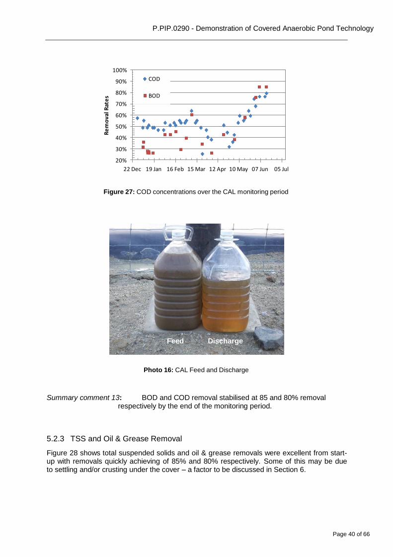
5.2.2 COD and BOD5 removal by the CAL
The COD and BOD removal rates were initially stable during start-up, decreased as a result of the conductivity shock but stabilised once normal operation was achieved. The data from the period of normal CAL operation shows 85% BOD and 80% COD removal, which match the CAL design values. Removal is shown visually in Photo 16. The CAL appears to perform similarly to an uncovered anaerobic pond at similar operating regimes.
Page 40 of 66
P.PIP.0290 - Demonstration of Covered Anaerobic Pond Technology
Re
mo
val R
ate
s
100%
90%
80%
70%
60%
50%
40%
30%
20%
COD
BOD
22 Dec 19 Jan 16 Feb 15 Mar 12 Apr 10 May 07 Jun 05 Jul
Figure 27: COD concentrations over the CAL monitoring period
Feed Discharge
Photo 16: CAL Feed and Discharge
Summary comment 13: BOD and COD removal stabilised at 85 and 80% removal respectively by the end of the monitoring period.
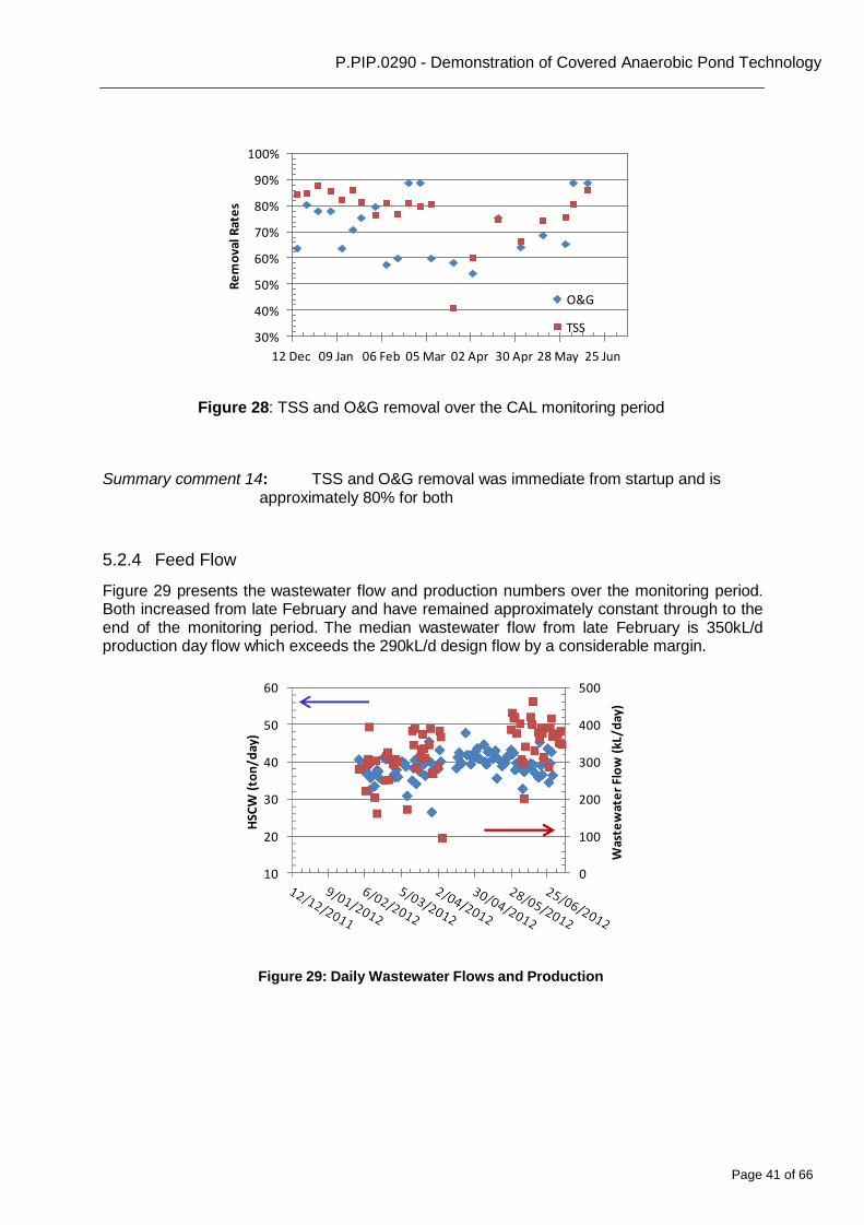
5.2.3 TSS and Oil & Grease Removal
Figure 28 shows total suspended solids and oil & grease removals were excellent from start- up with removals quickly achieving of 85% and 80% respectively. Some of this may be due to settling and/or crusting under the cover – a factor to be discussed in Section 6.
Page 41 of 66
P.PIP.0290 - Demonstration of Covered Anaerobic Pond Technology
Re
mo
val R
ate
s
HSC
W (
ton
/day
)
Was
tew
ate
r Fl
ow
(kL
/day
)
100%
90%
80%
70%
60%
50%
40%
30%
O&G
TSS
12 Dec 09 Jan 06 Feb 05 Mar 02 Apr 30 Apr 28 May 25 Jun
Figure 28: TSS and O&G removal over the CAL monitoring period
Summary comment 14: TSS and O&G removal was immediate from startup and is approximately 80% for both
5.2.4 Feed Flow
Figure 29 presents the wastewater flow and production numbers over the monitoring period. Both increased from late February and have remained approximately constant through to the end of the monitoring period. The median wastewater flow from late February is 350kL/d production day flow which exceeds the 290kL/d design flow by a considerable margin.
60 500
50 400
40 300
30 200
20 100
10 0
Figure 29: Daily Wastewater Flows and Production
Page 42 of 66
P.PIP.0290 - Demonstration of Covered Anaerobic Pond Technology
m3
bio
gas/
kg C
OD
re
mo
ved
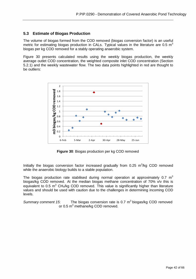
5.3 Estimate of Biogas Production
The volume of biogas formed from the COD removed (biogas conversion factor) is an useful metric for estimating biogas production in CALs. Typical values in the literature are 0.5 m3
biogas per kg COD removed for a stably operating anaerobic system.
Figure 30 presents calculated results using the weekly biogas production, the weekly average outlet COD concentration, the weighted composite inlet COD concentration (Section 5.2.1) and the weekly wastewater flow. The two data points highlighted in red are thought to be outliers:
2
1.8
1.6
1.4
1.2
1
0.8
0.6
0.4
0.2
0
6-Feb 5-Mar 2-Apr 30-Apr 28-May 25-Jun
Figure 30: Biogas production per kg COD removed
Initially the biogas conversion factor increased gradually from 0.25 m3/kg COD removed while the anaerobic biology builds to a stable population.
The biogas production rate stabilised during normal operation at approximately 0.7 m3
biogas/kg COD removed. At the median biogas methane concentration of 70% v/v this is
equivalent to 0.5 m3 CH4/kg COD removed. This value is significantly higher than literature values and should be used with caution due to the challenges in determining incoming COD levels.
Summary comment 15: The biogas conversion rate is 0.7 m3 biogas/kg COD removed
or 0.5 m3 methane/kg COD removed.
Page 43 of 66
P.PIP.0290 - Demonstration of Covered Anaerobic Pond Technology
6 Crust & Solids accumulation
Uncovered anaerobic ponds treating meat processing wastewater form often thick crusts over time due to the buoyant nature of the fine suspended solids in the wastewater and the tendency of oil & grease to separate into a floating scum. This is undesirable for CALs since the floating crust poses a risk to the integrity of the cover and the biogas capture system.
Settled solids also pose a risk to the longevity of the CAL, since they can rapidly accumulate and fill the pond, reducing the HRT available for treatment. The solids arise from two sources:
Inert suspended and gross solids originally present in the raw wastewater. Levels of
these solids need to be reduced through effective pre-treatment;
Biological solids formed during the anaerobic process. Although anaerobic processes are renown for their low sludge formation per tonne COD removed, large amounts of solids are still formed due to the high inlet organic load these ponds typically receive. Poor design can lead to rapid sludge build-up. CAL designs differ in how they handle this issue.
Pre-treatment of the raw wastewater at King Island consisted of a rotating wedgewire screen to remove gross and suspended solids. The original Dissolved Air Flotation (DAF) plant at King Island was badly corroded and JBS decided oil & grease levels were sufficiently low in the raw wastewater to avoid the need for a new DAF.
Crust build-up and sludge accumulation was investigated during the project after 2 and 6 months of operation.
6.1 Crust Build-up
An accumulation of a semi-solid floating scum under the cover was noted during the project. Table 5 reviews the visual observations through the two sample ports at the two inspection dates. Analysis of the scum sample from June 2012 is presented in Appendix C.
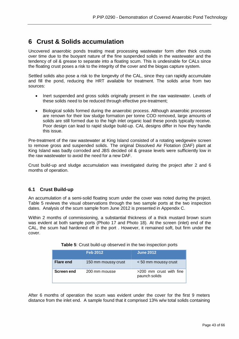
Within 2 months of commissioning, a substantial thickness of a thick mustard brown scum was evident at both sample ports (Photo 17 and Photo 18). At the screen (inlet) end of the CAL, the scum had hardened off in the port . However, it remained soft, but firm under the cover.
Table 5: Crust build-up observed in the two inspection ports
Feb 2012 June 2012
Flare end 150 mm moussy crust < 50 mm moussy crust
Screen end 200 mm mousse >200 mm crust with fine
paunch solids
After 6 months of operation the scum was evident under the cover for the first 9 meters distance from the inlet end. A sample found that it comprised 13% w/w total solids containing
Page 44 of 66
P.PIP.0290 - Demonstration of Covered Anaerobic Pond Technology
25% w/w oil and grease on a dry basis. This is consistent with a fatty deposit separating from the influent stream.
Photo 17: CAL crust at flare end Photo 18: CAL crust at screen end
In the outlet half of the CAL, the crust had thinned considerably since February and had a thin, mousse-like consistency. It is likely that much of the scum arises from a foamy mousse formed when the bacteria are under stress during the first 3 months of operation. As the pond has recovered and settled into normal operation, this scum will probably disappear – as is evident in the June sampling.
Nearer the inlet, however, there appears to be an issue with scum accumulation. The quantity of fat deposited over a 6 month period can be estimated from the median O&G influent concentration of 156mg/L, and assuming an O&G removal of 80% (see Figure 28) and flowrate of 350 kL/d. The remaining O&G translates to 5.6 tonnes of potential scum.
Summary Comment 16: Undesirable crust build-up is occurring beneath the cover with
greater than 200mm of semi-firm crust present within the inlet third of the CAL.
6.2 Sludge Accumulation
Sludge depth was measured using the Royce TSS meter calibrated to measure TSS levels. Sludge levels approximating greater than 1% w/v (e.g. 10,000 mg/l TSS) are detected when the unit goes off scale.
The sludge in the CAL has increased within the first 6 months of the CAL operation as shown in Table 6. The first 3 months saw a sludge depth of approximately 2 m increasing to 2.7m within the next 3 months. However, at both points, the Royce probe was able to easily transit through the sludge layer to the CAL base indicating that sludge was largely biological. Interpreting this finding is difficult since Johns Environmental has only recently applied this technology to CALs. Some sludge is essential to the normal operation of the pond, however, excessive quantities are undesirable. Further assessment is needed to determine this.
Page 45 of 66
P.PIP.0290 - Demonstration of Covered Anaerobic Pond Technology
Table 6: Sludge depth off the CAL base observed in the two inspection ports
Feb 2012 June 2012
Flare end 2.25m 2.7m
Screen end 2m 2.7m
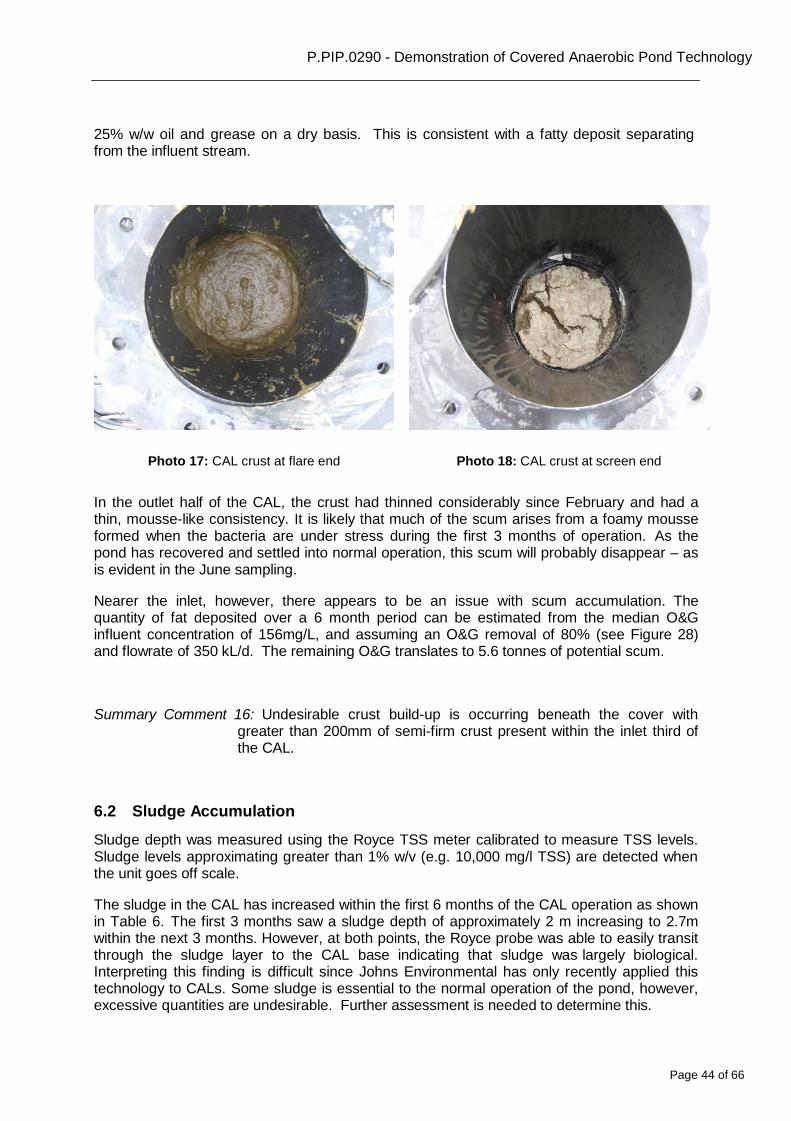
During the June 2012 sampling, a sludge truck successfully withdrew 10 m3 of black sludge through the sludge pipework over 15 minutes (Photo 19). There was little indication of rat holing (breakthrough of liquid) during the pumping since analysis of sludge sampled at even intervals during the withdrawal process showed little decrease in total solids with 2.7, 2.4, 2.4 and 2.2% total solids in sequential samples. Further analytical results are presented in Appendix C.
Photo 19: Sludge truck
Summary Comment 17: Sludge accumulation was evident in the CAL over 6 months of operation but was successfully withdrawn through the sludge removal piping.
Page 46 of 66
P.PIP.0290 - Demonstration of Covered Anaerobic Pond Technology
7 Conclusions
The major outcomes highlighted by this CAL monitoring study are presented below.
1. The CAL has operated successfully for 25 weeks post startup with excellent COD removal (80 %) which is the primary function of the pond, despite higher than design wastewater flows. The CAL delivers excellent biogas quality and quantity after 6
months of operation. Biogas production is approximately 0.7 m3/kg of COD removed
or 740 m3/day. The biogas methane concentration is consistently greater than 70% v/v.
2. Gas flow is reasonably steady over the full 7 day week despite the facility operating a
5 day/week.
3. Methane and CO2 are the main biogas constituents with lesser contaminants including nitrogen, argon, oxygen and H2S. H2S levels were typically 100 to 200 ppm during the production day, but as a concentration as high as 2,000 ppm (0.2%) was measured early in the production day.
4. CAL start-up required 25 weeks for stable operation. Initial startup was successful
within 8 weeks, despite the site being a greenfield site with no option for sludge inoculation.
5. A shock load of salt near the end phase of start-up severely upset the CAL with
noticeable impact on biogas production, VFA and alkalinity values and COD removal. This highlights the need for careful control of raw wastewater composition where a reliable and consistent supply of biogas is needed – for example for boiler fuel, or cogeneration in a gas engine.
6. The VFA/TA ratio proved an effective way of following the performance of the CAL but
is subject to time effective analysis.
7. Crust build up has occurred under the cover possibly due to the relatively low level of pretreatment used at King Island. The initial phase may be more due to microbial foaming than oil & grease accumulation and shows signs of thinning in the rear half of the CAL as it achieves normal performance. Near the inlet, however the scum is rich in oil & grease.
8. Sludge has also accumulated in the base of the CAL, but may be part of the
treatment process. A significant volume was successfully extracted using the sludge removal pipework after 6 months.
Page 47 of 66
P.PIP.0290 - Demonstration of Covered Anaerobic Pond Technology
8 Recommendations
1. The King Island CAL is operating at design performance and is producing sizeable volumes of methane rich biogas. The technology appears eminently appropriate for red meat processing plants.
2. There is a need for attentive management of raw wastewater feed composition and
variation compared to the traditional uncovered anaerobic ponds to ensure a reliable and steady supply of biogas for end-use. This will be financially important where biogas is recovered for gas engine cogeneration or for use as boiler fuel.
3. The risk of crust accumulation under the cover is clearly demonstrated at King Island.
This issue merits further attention to develop means by which potential damage to infrastructure is avoided.
4. Sludge withdrawal systems are recommended as a sludge management tool for
CALs.
5. The degree of error in methane concentration measured by in-line analysers caused by biogas moisture is unclear. There were large discrepancies in methane content measured by inline, portable and laboratory methane analysis. It would be helpful to quantify the impact of moisture on inline analysis for this critical measurement.
6. While pretreatment reduces the risk of crust build-up and sludge accumulation, it also
reduces potential for biogas formation with the lowered organic load. Recommended further research on the optimal degree of pretreatment would determine maximum biogas production while not hindering CAL performance.
7. Stormwater removal from the cover is a persistent problem in industrial CAL
operation. Attention to this detail in CAL cover design would benefit industry greatly.

Page 48 of 66
P.PIP.0290 - Demonstration of Covered Anaerobic Pond Technology
8. Appendices
Page 49 of 66
P.PIP.0290 - Demonstration of Covered Anaerobic Pond Technology
Appendix A: Monitoring Plan
This document proposes a plan [The Plan] for a 9-month investigation of the CAL operation. The Plan seeks to obtain sufficient factual information to achieve the stated objective.
Key Elements
The Plan will require the following field investigations to be conducted:
1. Characterisation of the volume and quality of effluent entering and leaving the CAL.
2. Characterisation of the volume and quality of the biogas leaving the CAL.
3. Sludge volumes produced and the utility of the sludge removal system in removing them.
Management of the Investigation
The skills required to perform the investigation require several contractors and consultants to be involved. The separate tasks and people involved are presented in Table 1.
Dr. Mike Johns of Johns Environmental [JEPL] will be project manager for the investigation and assist in on-site field work and training the Swift Australia King Island [SAKI] persons responsible for sampling and maintenance of the field equipment.
Dr Bronwen Butler (Johns Environmental) will assist in the investigation. She will collate, process and validate the field data supplied by and generate deliverables and communicate with SAKI personnel.
SAKI personnel will be responsible for monitoring and/or recording:
Daily flows to the CAL;
Inlet and outlet wastewater sampling (after training by Drs Johns and Butler);
Daily biogas flows;
Daily biogas composition (on-line methane analyser);
Plant data as required.
These data will be sent electronically to Johns Environmental in Brisbane for collation and processing.
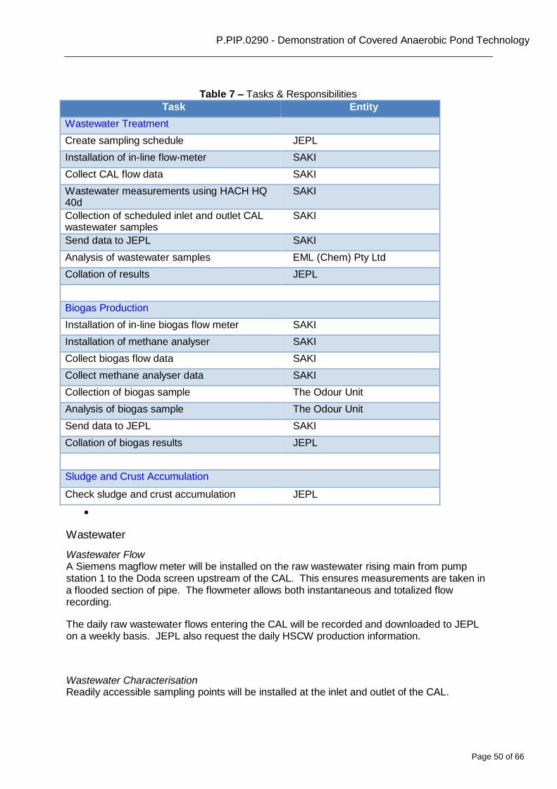
Page 50 of 66
P.PIP.0290 - Demonstration of Covered Anaerobic Pond Technology
Table 7 – Tasks & Responsibilities
Task Entity
Wastewater Treatment
Create sampling schedule JEPL
Installation of in-line flow-meter SAKI
Collect CAL flow data SAKI
Wastewater measurements using HACH HQ SAKI 40d Collection of scheduled inlet and outlet CAL SAKI wastewater samples Send data to JEPL SAKI
Analysis of wastewater samples EML (Chem) Pty Ltd
Collation of results JEPL
Biogas Production
Installation of in-line biogas flow meter SAKI
Installation of methane analyser SAKI
Collect biogas flow data SAKI
Collect methane analyser data SAKI
Collection of biogas sample The Odour Unit
Analysis of biogas sample The Odour Unit
Send data to JEPL SAKI
Collation of biogas results JEPL
Sludge and Crust Accumulation
Check sludge and crust accumulation JEPL
Wastewater
Wastewater Flow A Siemens magflow meter will be installed on the raw wastewater rising main from pump station 1 to the Doda screen upstream of the CAL. This ensures measurements are taken in a flooded section of pipe. The flowmeter allows both instantaneous and totalized flow recording.
The daily raw wastewater flows entering the CAL will be recorded and downloaded to JEPL on a weekly basis. JEPL also request the daily HSCW production information.
Wastewater Characterisation Readily accessible sampling points will be installed at the inlet and outlet of the CAL.
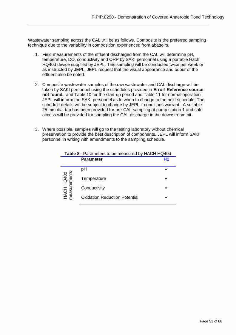
Page 51 of 66
P.PIP.0290 - Demonstration of Covered Anaerobic Pond Technology
HA
CH
HQ
40d
measure
me
nts
Wastewater sampling across the CAL will be as follows. Composite is the preferred sampling technique due to the variability in composition experienced from abattoirs.
1. Field measurements of the effluent discharged from the CAL will determine pH,
temperature, DO, conductivity and ORP by SAKI personnel using a portable Hach HQ40d device supplied by JEPL. This sampling will be conducted twice per week or as instructed by JEPL. JEPL request that the visual appearance and odour of the effluent also be noted.
2. Composite wastewater samples of the raw wastewater and CAL discharge will be
taken by SAKI personnel using the schedules provided in Error! Reference source not found. and Table 10 for the start-up period and Table 11 for normal operation. JEPL will inform the SAKI personnel as to when to change to the next schedule. The schedule details will be subject to change by JEPL if conditions warrant. A suitable 25 mm dia. tap has been provided for pre-CAL sampling at pump station 1 and safe access will be provided for sampling the CAL discharge in the downstream pit.
3. Where possible, samples will go to the testing laboratory without chemical
preservation to provide the best description of components. JEPL will inform SAKI personnel in writing with amendments to the sampling schedule.
Table 8– Parameters to be measured by HACH HQ40d
Parameter H1
pH
Temperature
Conductivity
Oxidation Reduction Potential
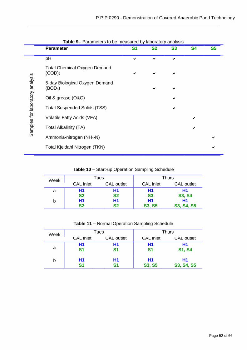
Page 52 of 66
P.PIP.0290 - Demonstration of Covered Anaerobic Pond Technology
Sa
mp
les f
or
labora
tory
analy
sis
Table 9– Parameters to be measured by laboratory analysis
Parameter S1 S2 S3 S4 S5
pH
Total Chemical Oxygen Demand (COD)t
5-day Biological Oxygen Demand (BOD5)
Oil & grease (O&G)
Total Suspended Solids (TSS)
Volatile Fatty Acids (VFA)
Total Alkalinity (TA)
Ammonia-nitrogen (NH3-N)
Total Kjeldahl Nitrogen (TKN)
Table 10 – Start-up Operation Sampling Schedule
Week
Tues Thurs
CAL inlet CAL outlet CAL inlet CAL outlet
a H1 S2
H1 S2
H1 S3
H1 S3, S4
b H1 S2
H1 S2
H1 S3, S5
H1 S3, S4, S5
Table 11 – Normal Operation Sampling Schedule
Week
Tues Thurs
CAL inlet CAL outlet CAL inlet CAL outlet
a H1 S1
H1 S1
H1 S1
H1 S1, S4
b
H1 S1
H1 S1
H1 S3, S5
H1 S3, S4, S5
Page 53 of 66
P.PIP.0290 - Demonstration of Covered Anaerobic Pond Technology
Biogas Monitoring
Biogas Flow The biogas train will be equipped with a FCI in-line gas flow meters. The SAKI personnel will collect this information and should also comment on the cover inflation and the colour of the flame. JEPL request for the information to be forwarded weekly.
Biogas Characterisation Biogas quality will be characterised. Methane content is the most critical component of the biogas in terms of end use. Off-line sampling permits contaminant levels in the gas to be known – these determine the extent of clean up required for specific uses.
1. The in-line methane analysis data will be collected by SAKI personnel from the
Draeger unit installed.
2. Biogas samples will be taken by The Odour Unit during normal operation period to analyse the biogas for CH3, CO2, H2S, NH3, N2O and CO content to permit comparison with data from sites involved in the A.ENV.0093 biogas quality study. The Odour Unit will analyse the samples using on-site equipment.
Sludge and Crust Accumulation
Crusting under the HDPE cover is highly undesirable. The development of crust will be assayed by inspection at access points in the cover. This will be performed by Dr Johns over the normal operation period when he is on site.
Sludge accumulation is also undesirable in the CAL. Sludge removal pipes have been installed on the floor of the CAL. These allow periodic sludge removal if necessary. Towards the end of the normal operation trial period Dr Johns will inspect the CAL to determine if sludge accumulation has occurred using both a Hydrolab Minisonde, a Royce meter and by pumping from the sludge collection system. An estimate of sludge accumulation will be made.
Demonstration of Covered Anaerobic Pond Technology
Page 54 of 66
Appendix B: Sample SCADA Biogas Output
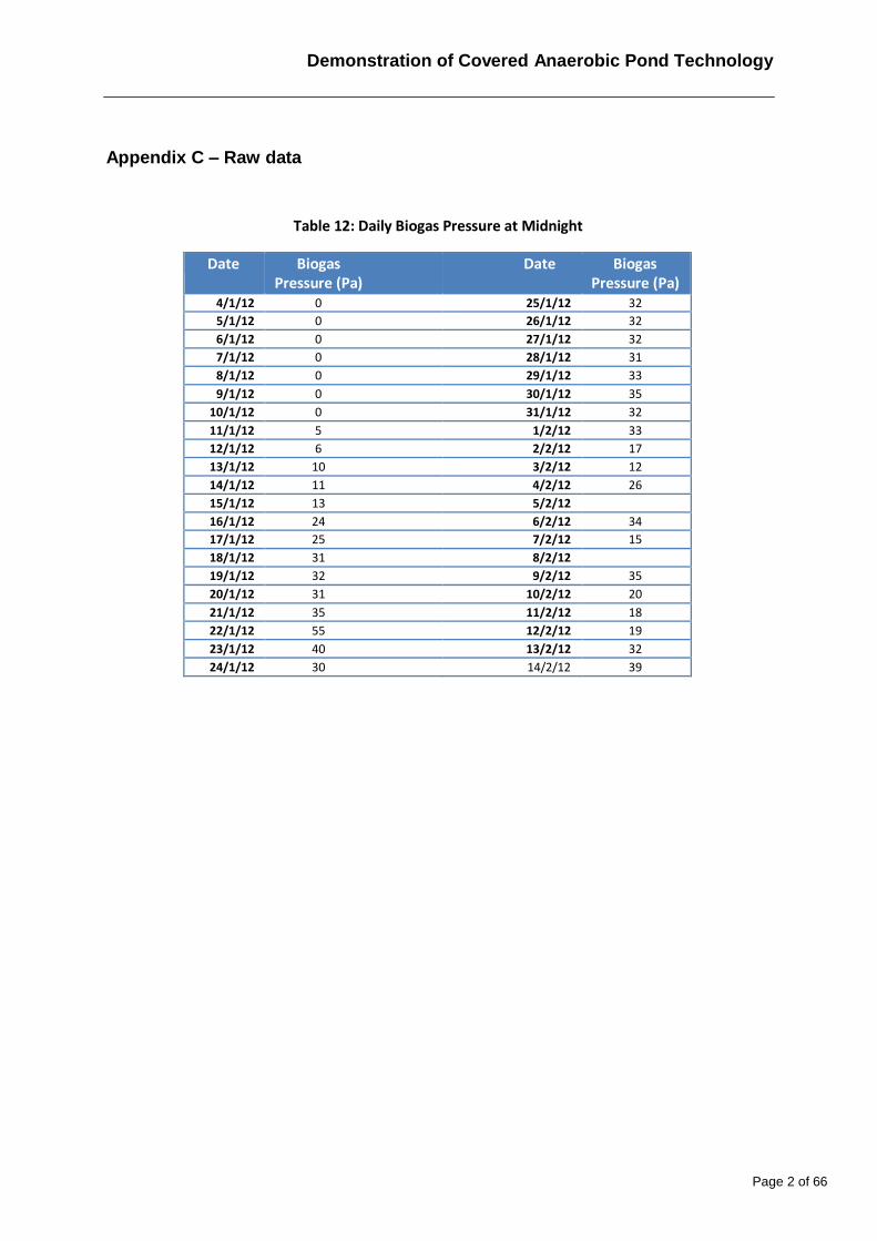
Demonstration of Covered Anaerobic Pond Technology
Page 2 of 66
Appendix C – Raw data
Table 12: Daily Biogas Pressure at Midnight
Date Biogas Pressure (Pa)
Date Biogas Pressure (Pa)
4/1/12 0 25/1/12 32
5/1/12 0 26/1/12 32
6/1/12 0 27/1/12 32
7/1/12 0 28/1/12 31
8/1/12 0 29/1/12 33
9/1/12 0 30/1/12 35
10/1/12 0 31/1/12 32
11/1/12 5 1/2/12 33
12/1/12 6 2/2/12 17
13/1/12 10 3/2/12 12
14/1/12 11 4/2/12 26
15/1/12 13 5/2/12 16/1/12 24 6/2/12 34
17/1/12 25 7/2/12 15
18/1/12 31 8/2/12 19/1/12 32 9/2/12 35
20/1/12 31 10/2/12 20
21/1/12 35 11/2/12 18
22/1/12 55 12/2/12 19
23/1/12 40 13/2/12 32
24/1/12 30 14/2/12 39
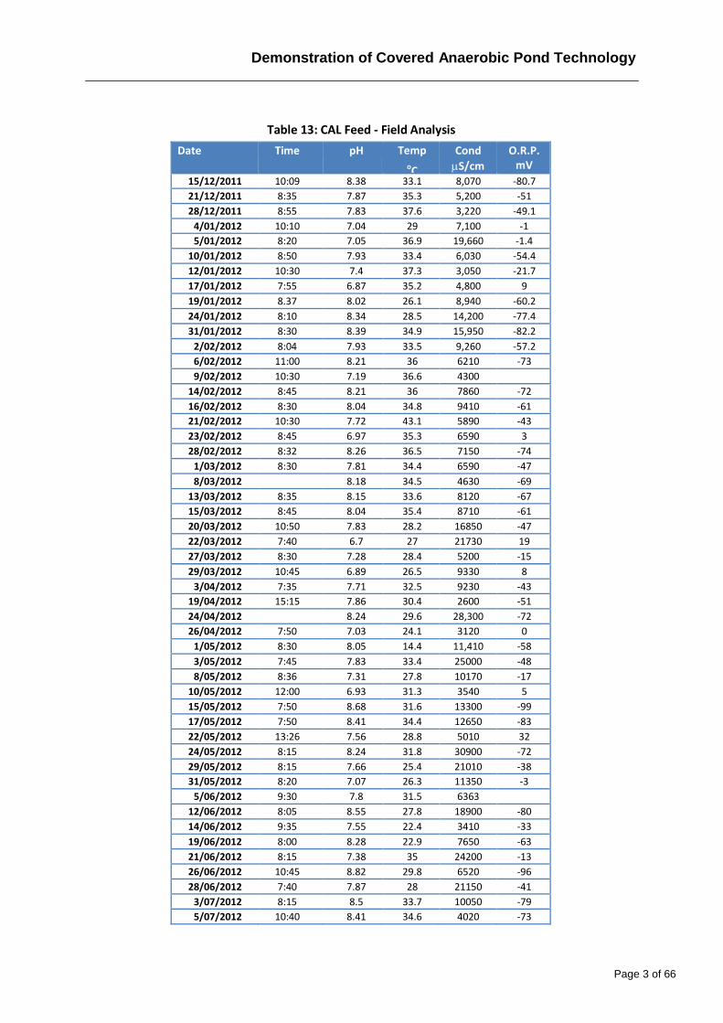
Demonstration of Covered Anaerobic Pond Technology
Page 3 of 66
Table 13: CAL Feed - Field Analysis
Date Time pH Temp oC
Cond
S/cm
O.R.P. mV
15/12/2011 10:09 8.38 33.1 8,070 -80.7
21/12/2011 8:35 7.87 35.3 5,200 -51
28/12/2011 8:55 7.83 37.6 3,220 -49.1
4/01/2012 10:10 7.04 29 7,100 -1
5/01/2012 8:20 7.05 36.9 19,660 -1.4
10/01/2012 8:50 7.93 33.4 6,030 -54.4
12/01/2012 10:30 7.4 37.3 3,050 -21.7
17/01/2012 7:55 6.87 35.2 4,800 9
19/01/2012 8.37 8.02 26.1 8,940 -60.2
24/01/2012 8:10 8.34 28.5 14,200 -77.4
31/01/2012 8:30 8.39 34.9 15,950 -82.2
2/02/2012 8:04 7.93 33.5 9,260 -57.2
6/02/2012 11:00 8.21 36 6210 -73
9/02/2012 10:30 7.19 36.6 4300 14/02/2012 8:45 8.21 36 7860 -72
16/02/2012 8:30 8.04 34.8 9410 -61
21/02/2012 10:30 7.72 43.1 5890 -43
23/02/2012 8:45 6.97 35.3 6590 3
28/02/2012 8:32 8.26 36.5 7150 -74
1/03/2012 8:30 7.81 34.4 6590 -47
8/03/2012 8.18 34.5 4630 -69
13/03/2012 8:35 8.15 33.6 8120 -67
15/03/2012 8:45 8.04 35.4 8710 -61
20/03/2012 10:50 7.83 28.2 16850 -47
22/03/2012 7:40 6.7 27 21730 19
27/03/2012 8:30 7.28 28.4 5200 -15
29/03/2012 10:45 6.89 26.5 9330 8
3/04/2012 7:35 7.71 32.5 9230 -43
19/04/2012 15:15 7.86 30.4 2600 -51
24/04/2012 8.24 29.6 28,300 -72
26/04/2012 7:50 7.03 24.1 3120 0
1/05/2012 8:30 8.05 14.4 11,410 -58
3/05/2012 7:45 7.83 33.4 25000 -48
8/05/2012 8:36 7.31 27.8 10170 -17
10/05/2012 12:00 6.93 31.3 3540 5
15/05/2012 7:50 8.68 31.6 13300 -99
17/05/2012 7:50 8.41 34.4 12650 -83
22/05/2012 13:26 7.56 28.8 5010 32
24/05/2012 8:15 8.24 31.8 30900 -72
29/05/2012 8:15 7.66 25.4 21010 -38
31/05/2012 8:20 7.07 26.3 11350 -3
5/06/2012 9:30 7.8 31.5 6363 12/06/2012 8:05 8.55 27.8 18900 -80
14/06/2012 9:35 7.55 22.4 3410 -33
19/06/2012 8:00 8.28 22.9 7650 -63
21/06/2012 8:15 7.38 35 24200 -13
26/06/2012 10:45 8.82 29.8 6520 -96
28/06/2012 7:40 7.87 28 21150 -41
3/07/2012 8:15 8.5 33.7 10050 -79
5/07/2012 10:40 8.41 34.6 4020 -73
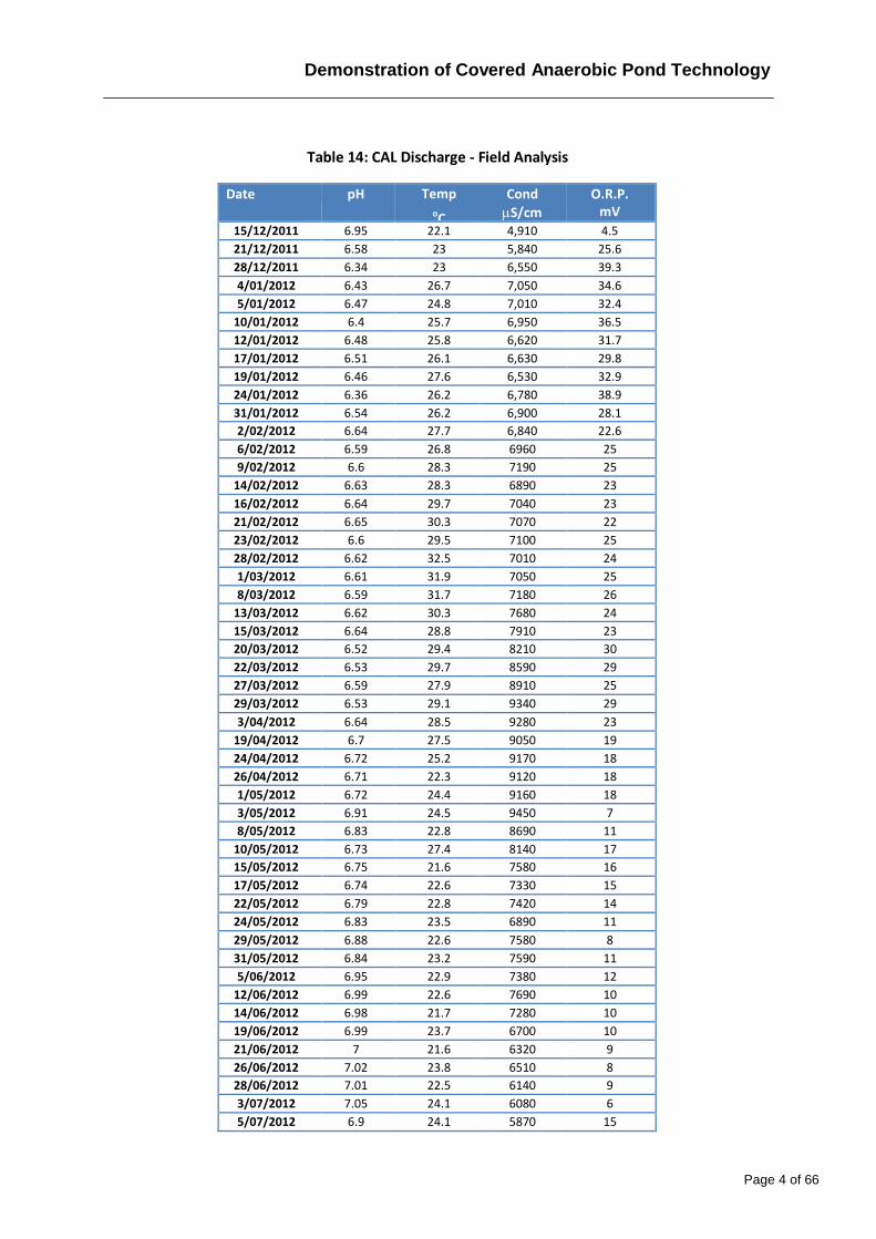
Demonstration of Covered Anaerobic Pond Technology
Page 4 of 66
Table 14: CAL Discharge - Field Analysis
Date pH Temp oC
Cond
S/cm
O.R.P. mV
15/12/2011 6.95 22.1 4,910 4.5
21/12/2011 6.58 23 5,840 25.6
28/12/2011 6.34 23 6,550 39.3
4/01/2012 6.43 26.7 7,050 34.6
5/01/2012 6.47 24.8 7,010 32.4
10/01/2012 6.4 25.7 6,950 36.5
12/01/2012 6.48 25.8 6,620 31.7
17/01/2012 6.51 26.1 6,630 29.8
19/01/2012 6.46 27.6 6,530 32.9
24/01/2012 6.36 26.2 6,780 38.9
31/01/2012 6.54 26.2 6,900 28.1
2/02/2012 6.64 27.7 6,840 22.6
6/02/2012 6.59 26.8 6960 25
9/02/2012 6.6 28.3 7190 25
14/02/2012 6.63 28.3 6890 23
16/02/2012 6.64 29.7 7040 23
21/02/2012 6.65 30.3 7070 22
23/02/2012 6.6 29.5 7100 25
28/02/2012 6.62 32.5 7010 24
1/03/2012 6.61 31.9 7050 25
8/03/2012 6.59 31.7 7180 26
13/03/2012 6.62 30.3 7680 24
15/03/2012 6.64 28.8 7910 23
20/03/2012 6.52 29.4 8210 30
22/03/2012 6.53 29.7 8590 29
27/03/2012 6.59 27.9 8910 25
29/03/2012 6.53 29.1 9340 29
3/04/2012 6.64 28.5 9280 23
19/04/2012 6.7 27.5 9050 19
24/04/2012 6.72 25.2 9170 18
26/04/2012 6.71 22.3 9120 18
1/05/2012 6.72 24.4 9160 18
3/05/2012 6.91 24.5 9450 7
8/05/2012 6.83 22.8 8690 11
10/05/2012 6.73 27.4 8140 17
15/05/2012 6.75 21.6 7580 16
17/05/2012 6.74 22.6 7330 15
22/05/2012 6.79 22.8 7420 14
24/05/2012 6.83 23.5 6890 11
29/05/2012 6.88 22.6 7580 8
31/05/2012 6.84 23.2 7590 11
5/06/2012 6.95 22.9 7380 12
12/06/2012 6.99 22.6 7690 10
14/06/2012 6.98 21.7 7280 10
19/06/2012 6.99 23.7 6700 10
21/06/2012 7 21.6 6320 9
26/06/2012 7.02 23.8 6510 8
28/06/2012 7.01 22.5 6140 9
3/07/2012 7.05 24.1 6080 6
5/07/2012 6.9 24.1 5870 15
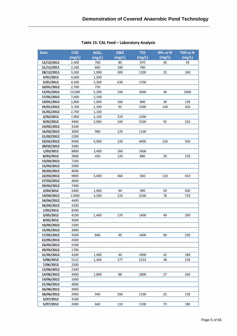
Demonstration of Covered Anaerobic Pond Technology
Page 5 of 66
Table 15: CAL Feed – Laboratory Analysis
Date COD (mg/L)
BOD5
(mg/L) O&G
(mg/L) TSS
(mg/L) NH3 as N (mg/L)
TKN as N (mg/L)
15/12/2011 2,400 700 80 970 36 39
21/12/2011 2,200 660 180 700 28/12/2011 3,500 1,900 300 1100 25 160
4/01/2012 4,600 1,500 5/01/2012 4,500 2,300 630 1700
10/01/2012 2,700 750 12/01/2012 13,000 5,200 100 2000 36 1000
17/01/2012 7,600 2,100 19/01/2012 2,800 1,000 160 800 28 130
24/01/2012 3,700 1,200 92 2300 140 320
31/01/2012 2,700 1,100 2/02/2012 7,800 2,100 370 2200 9/02/2012 4400 2,000 100 3100 92 310
14/02/2012 3100 16/02/2012 3000 980 120 1100 21/02/2012 2200 23/02/2012 9500 4,900 220 4400 150 350
28/02/2012 3300 1/03/2012 9800 3,400 260 1600 8/03/2012 2800 450 120 880 29 150
13/03/2012 7100 15/03/2012 2900 20/03/2012 4000 22/03/2012 9800 3,400 460 560 110 410
27/03/2012 4600 29/03/2012 7400 3/04/2012 5400 1,900 94 990 59 450
19/04/2012 11000 3,500 220 3100 78 720
24/04/2012 4400 26/04/2012 4200 1/05/2012 8200 3/05/2012 4100 1,400 270 1400 49 190
8/05/2012 4000 10/05/2012 2300 15/05/2012 3800 17/05/2012 3500 840 40 1400 90 230
22/05/2012 4300 24/05/2012 5500 29/05/2012 1700 31/05/2012 4200 1,400 40 1900 42 180
5/06/2012 5112 1,364 177 2233 38 234
7/06/2012 2500 12/06/2012 2300 14/06/2012 4400 1,800 88 1800 27 240
19/06/2012 1600 21/06/2012 4000 26/06/2012 4900 28/06/2012 2900 940 200 1100 25 130
3/07/2012 3100 5/07/2012 2400 660 110 1100 73 180
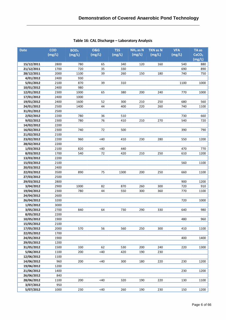
Demonstration of Covered Anaerobic Pond Technology
Page 6 of 66
Table 16: CAL Discharge – Laboratory Analysis
Date COD (mg/L)
BOD5
(mg/L) O&G
(mg/L) TSS
(mg/L) NH3 as N (mg/L)
TKN as N (mg/L)
VFA (mg/L)
TA as CaCO3
(mg/L)
15/12/2011 2800 780 65 340 120 160 540 880
21/12/2011 1700 720 35 330 690 890
28/12/2011 2000 1100 39 260 150 180 740 750
4/01/2012 2400 930 5/01/2012 2100 870 39 310 1100 1000
10/01/2012 2400 980 12/01/2012 2300 1000 65 380 200 240 770 1000
17/01/2012 2400 1000 19/01/2012 2400 1600 52 300 210 250 680 560
24/01/2012 2500 1400 44 400 220 260 740 1100
31/01/2012 2500 2/02/2012 2200 780 36 510 730 660
9/02/2012 2300 780 76 410 210 270 540 720
14/02/2012 2200 16/02/2012 2300 740 72 500 390 790
21/02/2012 2100 23/02/2012 2200 960 <40 410 230 280 550 1200
28/02/2012 2200 1/03/2012 2100 820 <40 440 470 770
8/03/2012 1700 540 72 420 210 250 610 1200
13/03/2012 2200 15/03/2012 2100 560 1100
20/03/2012 2400 22/03/2012 3500 890 75 1300 200 250 660 1100
27/03/2012 2500 29/03/2012 2800 900 1200
3/04/2012 2900 1000 82 870 260 300 720 910
19/04/2012 2300 780 44 550 300 360 770 1100
24/04/2012 2600 26/04/2012 3200 720 1000
1/05/2012 3000 3/05/2012 2700 840 64 730 290 330 640 980
8/05/2012 2200 10/05/2012 1900 480 960
15/05/2012 2100 17/05/2012 2000 570 56 560 250 300 410 1100
22/05/2012 1700 24/05/2012 1900 400 1400
29/05/2012 1200 31/05/2012 1500 330 62 530 200 240 220 1300
5/06/2012 1100 200 <40 420 190 230 12/06/2012 1100 14/06/2012 960 200 <40 300 180 220 230 1200
19/06/2012 1200 21/06/2012 1400 230 1200
26/06/2012 840 28/06/2012 1100 200 <40 320 190 220 130 1100
3/07/2012 950 5/07/2012 1000 230 <40 260 190 230 150 1200
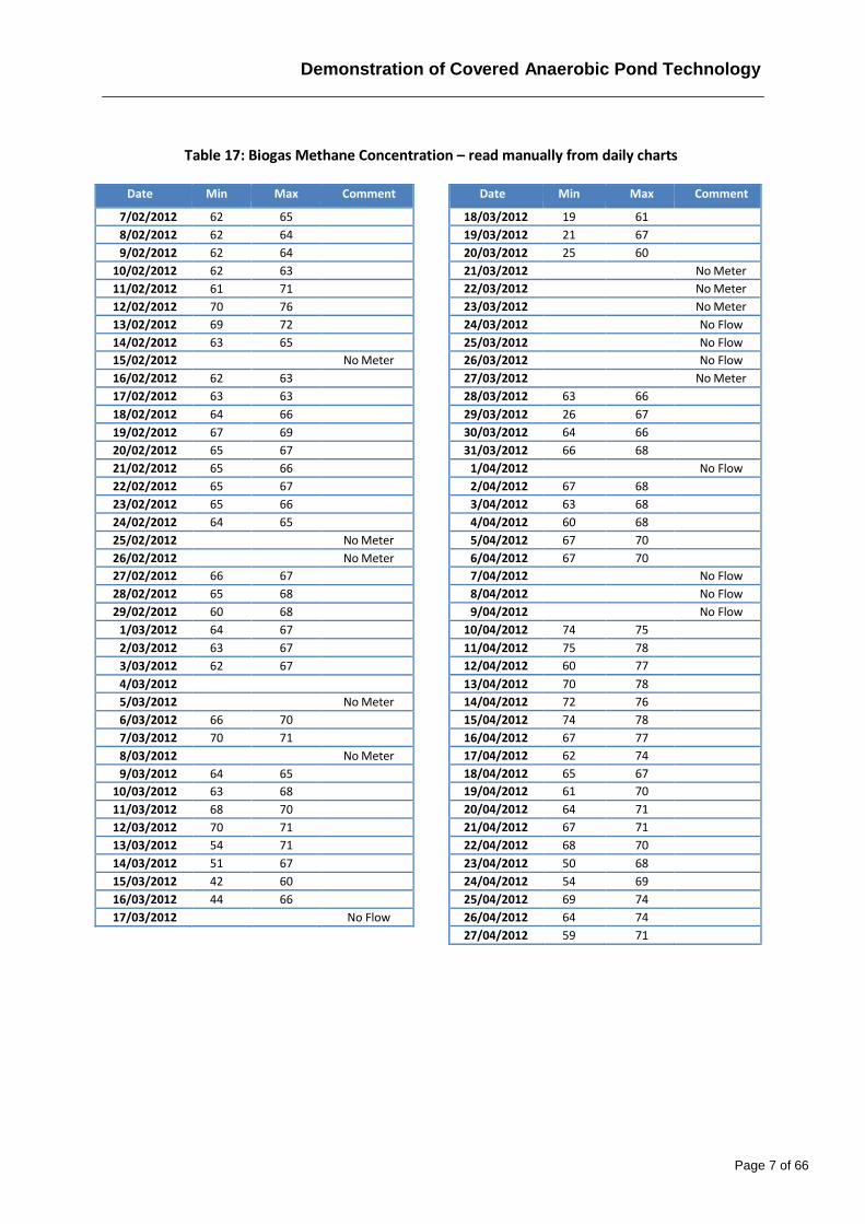
Demonstration of Covered Anaerobic Pond Technology
Page 7 of 66
Date Min Max Comment
18/03/2012 19 61 19/03/2012 21 67 20/03/2012 25 60 21/03/2012 No Meter
22/03/2012 No Meter
23/03/2012 No Meter
24/03/2012 No Flow
25/03/2012 No Flow
26/03/2012 No Flow
27/03/2012 No Meter
28/03/2012 63 66 29/03/2012 26 67 30/03/2012 64 66 31/03/2012 66 68
1/04/2012 No Flow
2/04/2012 67 68 3/04/2012 63 68 4/04/2012 60 68 5/04/2012 67 70 6/04/2012 67 70 7/04/2012 No Flow
8/04/2012 No Flow
9/04/2012 No Flow
10/04/2012 74 75 11/04/2012 75 78 12/04/2012 60 77 13/04/2012 70 78 14/04/2012 72 76 15/04/2012 74 78 16/04/2012 67 77 17/04/2012 62 74 18/04/2012 65 67 19/04/2012 61 70 20/04/2012 64 71 21/04/2012 67 71 22/04/2012 68 70 23/04/2012 50 68 24/04/2012 54 69 25/04/2012 69 74 26/04/2012 64 74 27/04/2012 59 71
Table 17: Biogas Methane Concentration – read manually from daily charts
Date Min Max Comment
7/02/2012 62 65 8/02/2012 62 64 9/02/2012 62 64
10/02/2012 62 63 11/02/2012 61 71 12/02/2012 70 76 13/02/2012 69 72 14/02/2012 63 65 15/02/2012 No Meter
16/02/2012 62 63 17/02/2012 63 63 18/02/2012 64 66 19/02/2012 67 69 20/02/2012 65 67 21/02/2012 65 66 22/02/2012 65 67 23/02/2012 65 66 24/02/2012 64 65 25/02/2012 No Meter
26/02/2012 No Meter
27/02/2012 66 67 28/02/2012 65 68 29/02/2012 60 68
1/03/2012 64 67 2/03/2012 63 67 3/03/2012 62 67 4/03/2012
5/03/2012 No Meter
6/03/2012 66 70 7/03/2012 70 71 8/03/2012 No Meter
9/03/2012 64 65 10/03/2012 63 68 11/03/2012 68 70 12/03/2012 70 71 13/03/2012 54 71 14/03/2012 51 67 15/03/2012 42 60 16/03/2012 44 66 17/03/2012 No Flow
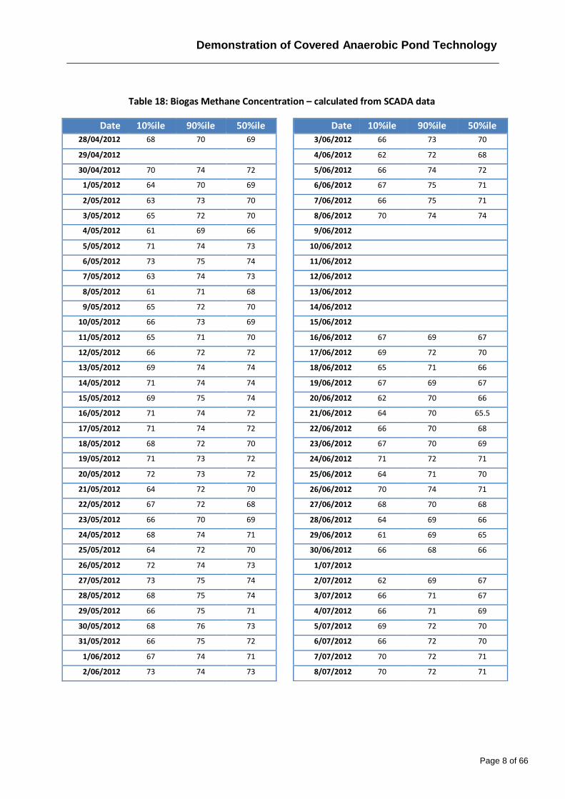
Demonstration of Covered Anaerobic Pond Technology
Page 8 of 66
Date 10%ile 90%ile 50%ile
3/06/2012 66 73 70
4/06/2012 62 72 68
5/06/2012 66 74 72
6/06/2012 67 75 71
7/06/2012 66 75 71
8/06/2012 70 74 74
9/06/2012
10/06/2012
11/06/2012
12/06/2012
13/06/2012
14/06/2012
15/06/2012
16/06/2012 67 69 67
17/06/2012 69 72 70
18/06/2012 65 71 66
19/06/2012 67 69 67
20/06/2012 62 70 66
21/06/2012 64 70 65.5
22/06/2012 66 70 68
23/06/2012 67 70 69
24/06/2012 71 72 71
25/06/2012 64 71 70
26/06/2012 70 74 71
27/06/2012 68 70 68
28/06/2012 64 69 66
29/06/2012 61 69 65
30/06/2012 66 68 66
1/07/2012
2/07/2012 62 69 67
3/07/2012 66 71 67
4/07/2012 66 71 69
5/07/2012 69 72 70
6/07/2012 66 72 70
7/07/2012 70 72 71
8/07/2012 70 72 71
Table 18: Biogas Methane Concentration – calculated from SCADA data
Date 10%ile 90%ile 50%ile
28/04/2012 68 70 69
29/04/2012
30/04/2012 70 74 72
1/05/2012 64 70 69
2/05/2012 63 73 70
3/05/2012 65 72 70
4/05/2012 61 69 66
5/05/2012 71 74 73
6/05/2012 73 75 74
7/05/2012 63 74 73
8/05/2012 61 71 68
9/05/2012 65 72 70
10/05/2012 66 73 69
11/05/2012 65 71 70
12/05/2012 66 72 72
13/05/2012 69 74 74
14/05/2012 71 74 74
15/05/2012 69 75 74
16/05/2012 71 74 72
17/05/2012 71 74 72
18/05/2012 68 72 70
19/05/2012 71 73 72
20/05/2012 72 73 72
21/05/2012 64 72 70
22/05/2012 67 72 68
23/05/2012 66 70 69
24/05/2012 68 74 71
25/05/2012 64 72 70
26/05/2012 72 74 73
27/05/2012 73 75 74
28/05/2012 68 75 74
29/05/2012 66 75 71
30/05/2012 68 76 73
31/05/2012 66 75 72
1/06/2012 67 74 71
2/06/2012 73 74 73
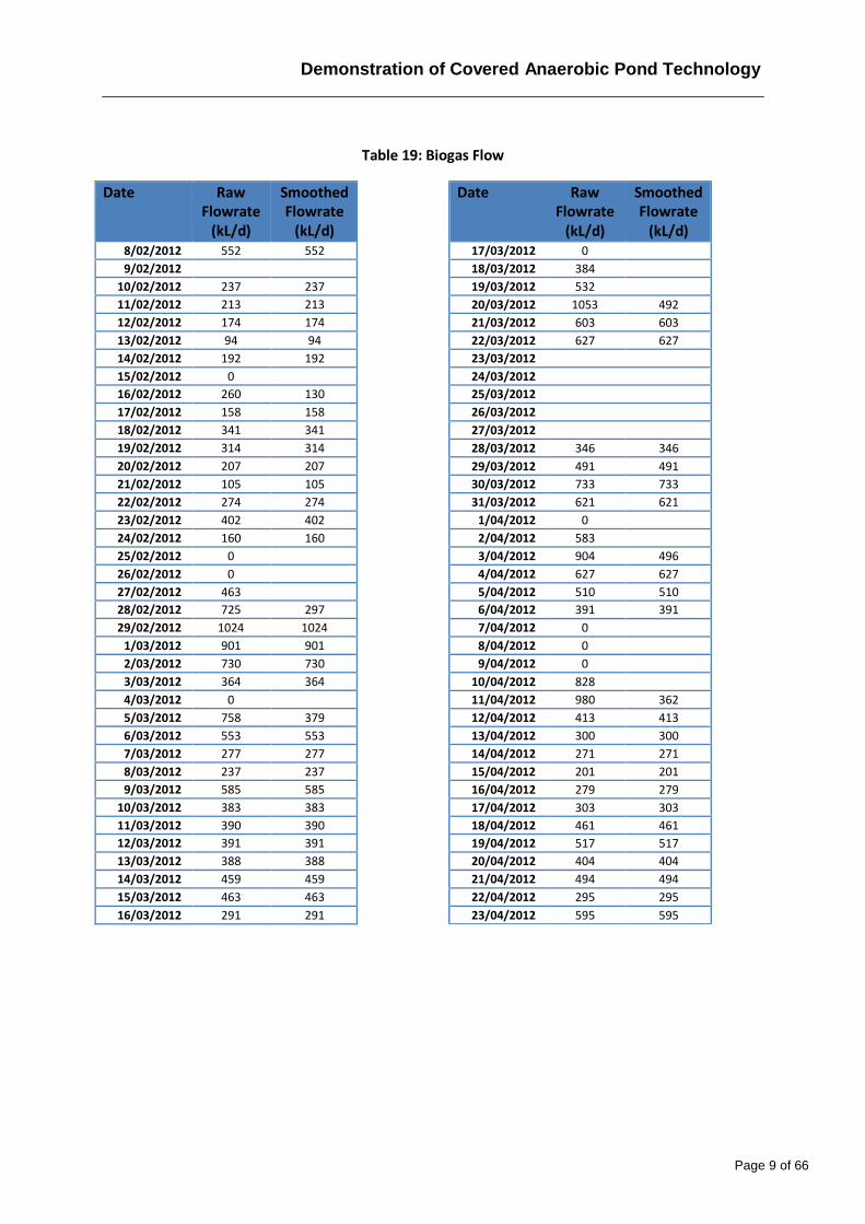
Demonstration of Covered Anaerobic Pond Technology
Page 9 of 66
Date Raw Flowrate
(kL/d)
Smoothed Flowrate
(kL/d) 17/03/2012 0 18/03/2012 384 19/03/2012 532 20/03/2012 1053 492
21/03/2012 603 603
22/03/2012 627 627
23/03/2012
24/03/2012
25/03/2012
26/03/2012
27/03/2012
28/03/2012 346 346
29/03/2012 491 491
30/03/2012 733 733
31/03/2012 621 621
1/04/2012 0 2/04/2012 583 3/04/2012 904 496
4/04/2012 627 627
5/04/2012 510 510
6/04/2012 391 391
7/04/2012 0 8/04/2012 0 9/04/2012 0
10/04/2012 828 11/04/2012 980 362
12/04/2012 413 413
13/04/2012 300 300
14/04/2012 271 271
15/04/2012 201 201
16/04/2012 279 279
17/04/2012 303 303
18/04/2012 461 461
19/04/2012 517 517
20/04/2012 404 404
21/04/2012 494 494
22/04/2012 295 295
23/04/2012 595 595
Table 19: Biogas Flow
Date Raw Flowrate
(kL/d)
Smoothed Flowrate
(kL/d) 8/02/2012 552 552
9/02/2012
10/02/2012 237 237
11/02/2012 213 213
12/02/2012 174 174
13/02/2012 94 94
14/02/2012 192 192
15/02/2012 0 16/02/2012 260 130
17/02/2012 158 158
18/02/2012 341 341
19/02/2012 314 314
20/02/2012 207 207
21/02/2012 105 105
22/02/2012 274 274
23/02/2012 402 402
24/02/2012 160 160
25/02/2012 0 26/02/2012 0 27/02/2012 463 28/02/2012 725 297
29/02/2012 1024 1024
1/03/2012 901 901
2/03/2012 730 730
3/03/2012 364 364
4/03/2012 0 5/03/2012 758 379
6/03/2012 553 553
7/03/2012 277 277
8/03/2012 237 237
9/03/2012 585 585
10/03/2012 383 383
11/03/2012 390 390
12/03/2012 391 391
13/03/2012 388 388
14/03/2012 459 459
15/03/2012 463 463
16/03/2012 291 291
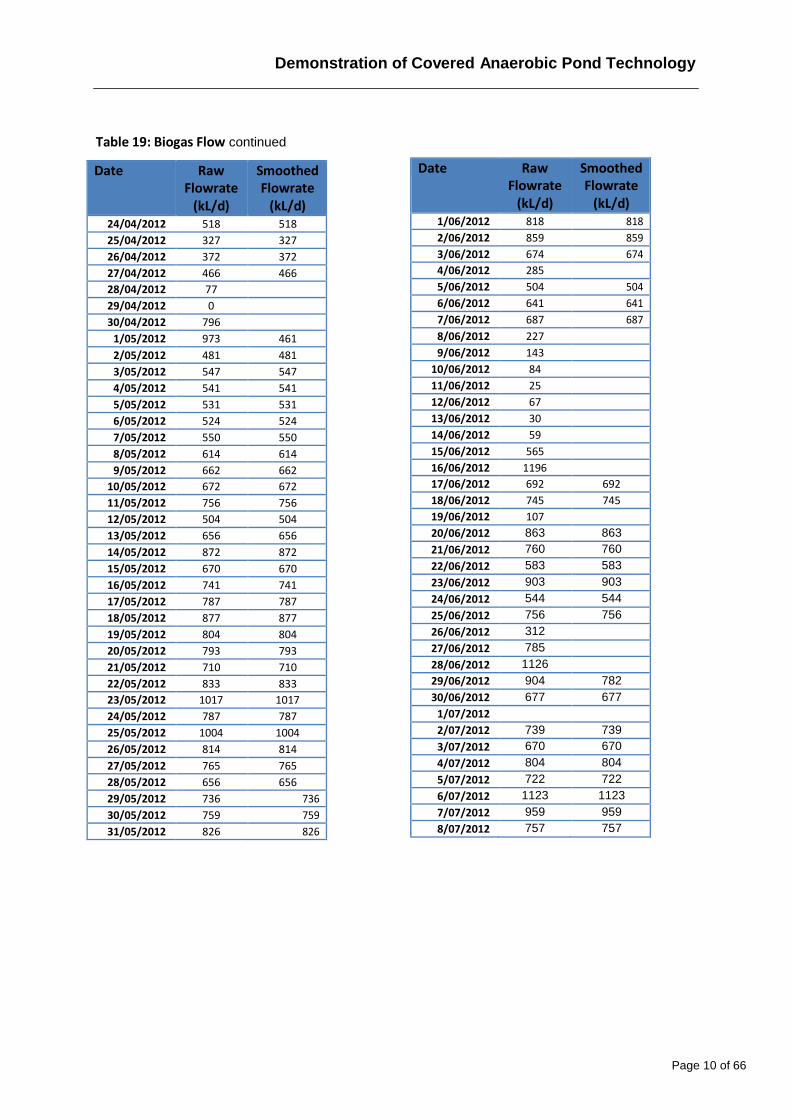
Demonstration of Covered Anaerobic Pond Technology
Page 10 of 66
Date Raw Flowrate
(kL/d)
Smoothed Flowrate
(kL/d) 1/06/2012 818 818
2/06/2012 859 859
3/06/2012 674 674
4/06/2012 285 5/06/2012 504 504
6/06/2012 641 641
7/06/2012 687 687
8/06/2012 227 9/06/2012 143
10/06/2012 84 11/06/2012 25 12/06/2012 67 13/06/2012 30 14/06/2012 59 15/06/2012 565 16/06/2012 1196 17/06/2012 692 692
18/06/2012 745 745
19/06/2012 107 20/06/2012 863 863
21/06/2012 760 760
22/06/2012 583 583
23/06/2012 903 903
24/06/2012 544 544
25/06/2012 756 756
26/06/2012 312 27/06/2012 785 28/06/2012 1126 29/06/2012 904 782
30/06/2012 677 677
1/07/2012
2/07/2012 739 739
3/07/2012 670 670
4/07/2012 804 804
5/07/2012 722 722
6/07/2012 1123 1123
7/07/2012 959 959
8/07/2012 757 757
Table 19: Biogas Flow continued
Date Raw Flowrate
(kL/d)
Smoothed Flowrate
(kL/d) 24/04/2012 518 518
25/04/2012 327 327
26/04/2012 372 372
27/04/2012 466 466
28/04/2012 77 29/04/2012 0 30/04/2012 796
1/05/2012 973 461
2/05/2012 481 481
3/05/2012 547 547
4/05/2012 541 541
5/05/2012 531 531
6/05/2012 524 524
7/05/2012 550 550
8/05/2012 614 614
9/05/2012 662 662
10/05/2012 672 672
11/05/2012 756 756
12/05/2012 504 504
13/05/2012 656 656
14/05/2012 872 872
15/05/2012 670 670
16/05/2012 741 741
17/05/2012 787 787
18/05/2012 877 877
19/05/2012 804 804
20/05/2012 793 793
21/05/2012 710 710
22/05/2012 833 833
23/05/2012 1017 1017
24/05/2012 787 787
25/05/2012 1004 1004
26/05/2012 814 814
27/05/2012 765 765
28/05/2012 656 656
29/05/2012 736 736
30/05/2012 759 759
31/05/2012 826 826
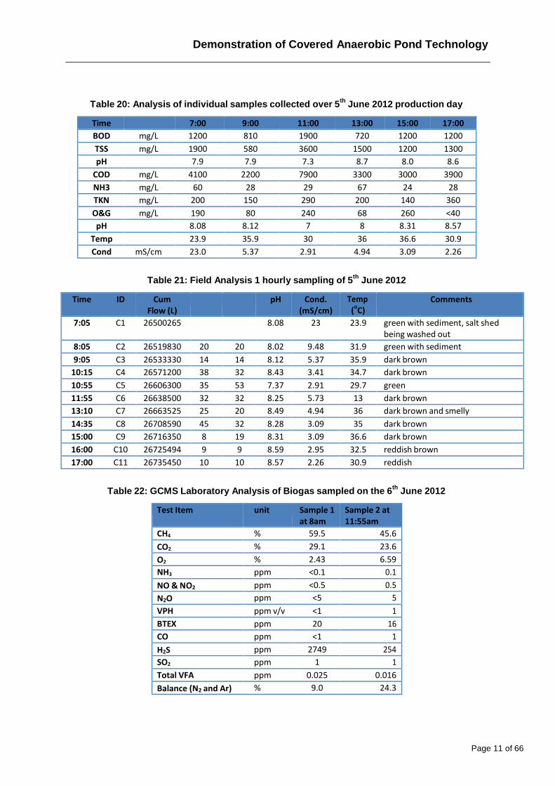
Demonstration of Covered Anaerobic Pond Technology
Page 11 of 66
Table 20: Analysis of individual samples collected over 5th
June 2012 production day
Time 7:00 9:00 11:00 13:00 15:00 17:00
BOD mg/L 1200 810 1900 720 1200 1200
TSS mg/L 1900 580 3600 1500 1200 1300
pH 7.9 7.9 7.3 8.7 8.0 8.6
COD mg/L 4100 2200 7900 3300 3000 3900
NH3 mg/L 60 28 29 67 24 28
TKN mg/L 200 150 290 200 140 360
O&G mg/L 190 80 240 68 260 <40
pH 8.08 8.12 7 8 8.31 8.57
Temp 23.9 35.9 30 36 36.6 30.9
Cond mS/cm 23.0 5.37 2.91 4.94 3.09 2.26
Table 21: Field Analysis 1 hourly sampling of 5th
June 2012
Time ID Cum Flow (L)
pH Cond. (mS/cm)
Temp (
oC)
Comments
7:05 C1 26500265 8.08 23 23.9 green with sediment, salt shed being washed out
8:05 C2 26519830 20 20 8.02 9.48 31.9 green with sediment
9:05 C3 26533330 14 14 8.12 5.37 35.9 dark brown
10:15 C4 26571200 38 32 8.43 3.41 34.7 dark brown
10:55 C5 26606300 35 53 7.37 2.91 29.7 green
11:55 C6 26638500 32 32 8.25 5.73 13 dark brown
13:10 C7 26663525 25 20 8.49 4.94 36 dark brown and smelly
14:35 C8 26708590 45 32 8.28 3.09 35 dark brown
15:00 C9 26716350 8 19 8.31 3.09 36.6 dark brown
16:00 C10 26725494 9 9 8.59 2.95 32.5 reddish brown
17:00 C11 26735450 10 10 8.57 2.26 30.9 reddish
Table 22: GCMS Laboratory Analysis of Biogas sampled on the 6th
June 2012
Test Item unit Sample 1 at 8am
Sample 2 at 11:55am
CH4 % 59.5 45.6
CO2 % 29.1 23.6
O2 % 2.43 6.59
NH3 ppm <0.1 0.1
NO & NO2 ppm <0.5 0.5
N2O ppm <5 5
VPH ppm v/v <1 1
BTEX ppm 20 16
CO ppm <1 1
H2S ppm 2749 254
SO2 ppm 1 1
Total VFA ppm 0.025 0.016
Balance (N2 and Ar) % 9.0 24.3

Demonstration of Covered Anaerobic Pond Technology
Page 12 of 66
Table 23: CAL Crust analysis from 5 June samples
Screen port
Flare port
TS %w/w RB 13 10.9
Fixed TS %w/w DB 14.9 17.6
Org. TS %w/w DB 85.1 82.4
TKN mg/kg DB 14,000 32,000
NO2 as N mg/kg DB <250 <250
NO3 as N mg/kg DB <5 <5
TN as N mg/kg DB
TP as P mg/kg DB 2,500 4,400
O&G mg/kg DB 24,000 25,000
Table 24: CAL sludge analysis from 5 June samples
CAL CAL CAL CAL Sludge A Sludge B Sludge C Sludge D
TS %w/w RB 2.65 2.39 2.38 2.22
Fixed TS %w/w DB 30.4 29.8 30.8 30.8
Org. TS %w/w DB 69.6 70.2 69.2 69.2
TKN mg/kg DB 49,000 45,000 55,000 52,000
NO2 as N mg/kg DB <250 <250 <250 <250
NO3 as N mg/kg DB <5 <5 <5 <5
TN as N mg/kg DB 49,000 45,000
TP as P mg/kg DB 7,600 7,000 7,300 8,300
O&G mg/kg DB
TDS mg/L 4,400 4,500 4,400 4,400


![Template Hui RMAP FLYER [FINAL] 2020.08hopeserviceshawaii.org/.../02/Template-Hui-RMAP-FLYER-FINAL-202… · Template Hui RMAP FLYER [FINAL] 2020.08.20 Author: Kristen Alice Apruzzese](https://static.fdocuments.in/doc/165x107/601e135045d448438a01e950/template-hui-rmap-flyer-final-2020-template-hui-rmap-flyer-final-20200820.jpg)