Final Report for TWDB Contract No. 0904830899

Sediment Transport Modeling of Reach Scale Geomorphic Processes

J.K. Haschenburger University of Texas at San Antonio

and

Joanna Curran University of Virginia

January 22, 2012

1 INTRODUCTION This study investigated the use of a modeling strategy to predict channel adjustment and floodplain accretion in the lower San Antonio River. The modeling strategy was employed in three subreaches with different channel characteristics to capture a range of possible geomorphic responses in the river and validated with empirical observations where possible. Using the modeling strategy, flow simulations of prescribed in-stream flows can provide initial insights into the response of the river.

This report is divided into six sections. The next section on empirical observations describes the selected study reaches, outlines the methodology employed to collect and analyze field observations, and reports on key empirical trends from the analysis of the observations. The third and fourth sections are devoted to the development and initial testing of modeling strategies for channel adjustment and floodplain accretion, respectively. Concluding comments regarding the use and further development of the models are outlined in the last section.

2 EMPIRICAL DATABASE

2.1 Study Reach Selection Three reaches were selected based on field reconnaissance of the San Antonio River from the Elmendorf area to south of Goliad. The three reaches are identified as Floresville (Figure 1), Charco (Figure 2), and Goliad (Figure 3). The overriding selection criteria were channel morphology characteristics and points of land access to the river. Previous research on the general characteristics of the San Antonio River by Engel and Curran (2008) helped guide reach selection.

2.2 Existing River Observations and Analysis

2.2.1 Flow and Sediment Transport Streamflow records of discharge characteristics are available at several US Geological Survey (USGS) gauging stations within the general study area (Elmendorf 08181800, Floresville 08183200, Falls City 08183500, and Goliad 08188500). The hydrological forcing responsible for sediment transport were quantified by using these streamflow observations. First, stage-discharge rating curves were used to assign discharges to periods of sediment transport sampling. Second, flow duration analysis was completed based on mean daily discharge to determine the frequency of occurrence of the flow rates sampled for sediment transport.

Observations of suspended sediment concentration and suspended load are available for the Elmendorf, Falls City, and Goliad gauging stations. The Elmendorf suspended sediment concentration rating curve shows the most pronounced difference among the USGS data.

2

Figure 1. The Floresville reach. Locations of channel cross-sectional survey and boundary material sampling shown by circles. Location of USGS streamflow gauging and sediment transport measurements shown by square.

3

Figure 2. The Charco reach. Locations of channel cross-sectional survey and boundary material sampling shown by circles. Location of sediment transport measurements upstream near Kenedy.

4

Figure 3. The Goliad reach. Locations of channel cross-sectional survey and boundary material sampling shown by circles. Location of USGS streamflow gauging and sediment transport measurements shown by square.

5

2.2.2 Channel Change Cawthon and Curran (2007) quantified changes to the planform geometry and channel width of the lower San Antonio River through a GIS analysis of aerial photography spanning from 1938 to 2004. In an analysis of lateral erosion, the lower San Antonio River exhibited a spatially consistent trend of channel widening over the study period, with the median channel width increasing by 82 ft for an overall reach rate of 1.2 ft yr-1

(Table 1). In the upper portion of the study reach, more than half of the total channel widening occurred between 1938 and 1948 when the median channel width increased from 82 to 132 ft. This was hypothesized to be a result of bank slumping following the 1946 flood. After 1948, channel width increased by another 30 ft. In the lower portion of the study reach, channel width increased by 85 ft from an average width of 108 to 193 ft between 1940 and 2004. The difference in the timing of channel widening between the upper and lower reaches appeared to result, in part, from the different soil characteristics in the two reaches.

Table 1. Rates of channel adjustment Aerial photography Cross-sectional survey

Rate of Rate of Rate of Time width Time width cross-sectional

Reach period

(yr) increase (ft yr-1) Site

period (yr)

increase (ft yr-1)

change (ft2 yr -1)

Upper 66 2.4 1 87 1.1 8.4 Lower 64 1.3 2 57 1.6 11.2

Available information on bed aggradation or degradation is more limited with only two known sites with surveyed channel cross sections in the area (Table 1). Site 1 is the FM 775 bridge at river mile 30 near Floresville, while site 2 is at the FM 791 bridge near Falls City at river mile 62.5. These cross sections are associated with USGS streamflow gauging stations. For the 2007 study, the cross sections were re-surveyed at the USGS gauges to quantify channel erosion, deposition, and movement since the time the original cross section was measured during gauge installation. Bridge handrails were included in the original cross sections and were used as the datum for the resurvey.

At site 1 the original cross-sectional survey was completed in 1920 on the downstream side of an old bridge adjacent to the current FM 775 bridge (Figure 4). Between 1920 and 2007, the channel migrated 95 ft for an average rate of 1.1 ft yr-1. The channel cross-sectional area increased by 55% from 900 ft2 to 1630 ft2, which was accommodated by an increase in channel width of 40 ft and incision of 1.0 ft.

6

Figure 4. Cross-sectional change recorded by survey at site 1

At site 2, the original cross section is from 1950 on the upstream side of the current FM 791 bridge (Figure 5). Although the time frame is reduced compared to site 1, channel width increased by 40 ft. Channel incision was four times as large at this location. Maximum channel depth increased by 4 ft, allowing for a 67% increase in channel area from 1340 ft2 to 1981 ft2.

Figure 5. Cross-sectional change recorded by survey at site 2

Although averaging changes in channel adjustment over long time periods (Table 1) can mask short-term changes, these empirical rates provide a means to estimate volumetric rates of channel change over the Floresville reach. Applying the rate of cross-sectional change of 8.4 ft2yr-1 over the Floresville reach, a length of 16,273 ft, gives a volumetric rate of 136,696 ft3yr-1, which can be converted to 11,307 tons.

2.3 New Field Observations and Analysis

2.3.1 Cross-sectional Survey Each reach was characterized by at least 5 cross sections. Streamwise spacing was set to meet minimum requirements for HEC-RAS modeling and achieve a relatively consistent study reach length based on the number of bankfull widths (i.e., 22.8 ± 3.9 for the three reaches). An initial streamwise position was selected at one site with land access to the river with other positions guided by the spacing interval. Cross-sectional survey captured major breaks in slope along each cross section. Latitude and longitude coordinates were established by collecting and differentially correcting a benchmarked observation using a GPS unit. Where land access was not possible, survey of the flow channel was extended to the floodplain using available LiDAR coverage.

7

2.3.2 Boundary Materials Sediment samples were collected along each cross section. All samples were collected by a grab technique and therefore represent near surface sediments. In general, characteristics of sediments are based on between 4 to 10 samples of streambed sediments depending on channel bed width, 6 samples of bank sediments (3 per bank), and 6 samples of floodplain sediments where possible (3 per surface).

All sediments were wet sieved to remove fines (<0.0025 in.) that aggregate and therefore bias the grain size distribution. The remaining coarser sediments were dry sieved. Size fractions were characterized by 0.5 phi increments. The grain size distribution for a given depositional environment was calculated as a weighted mean to represent the boundary materials of the cross section.

2.3.3 Suspended Load Suspended sediment observations were collected by deploying a depth-integrating DH-76 suspended sediment sampler. Collection proceeded using a fixed width interval along the cross section aiming for 20 samples. Nonetheless, a few 10 sample efforts were completed early in the field program to ensure at least some observations given the unpredictability of floods. Sampling suspended sediment was a lower priority given the availability of USGS observations, so it followed bedload sampling throughout most of the field program. For a given sampling, transit rates for the DH-76 were determined for the specific flow condition and then held constant. Derived rates in this study correspond to a range in flow duration exceedence of 2 to 48% and 6 to 22% for Floresville and Goliad, respectively.

Sediment concentrations were determined in the lab by quantifying the mass of water and sediment and assuming a water density of 62.4 lb ft-3. Suspended sediment loads are the product of the mean cross-sectional concentration of suspended sediment and mean flow discharge over the sampling period. Reported values are representative of the sampling cross section. These data were combined with USGS data where appropriate. Rating curves were fitted using least squares regression. No grain size analysis was undertaken for suspended sediments. However, limited analysis of USGS observations at Falls City and Goliad suggest that sizes <0.0025 in. dominate over most flow rates sampled.

2.3.4 Bedload Bedload observations were collected by deploying a 3 inch orifice Helley-Smith bedload sampler with a 0.0079 in. mesh collection bag from the nearest workable bridge. The orifice size was sufficiently large relative to the largest grain sizes present locally on the streambed to permit capture of all potentially mobile grain sizes.

Collection proceeded using a fixed width interval strategy along the cross section aiming for 20 samples. Nonetheless, early in the sampling program, a few 10 sample efforts were completed to ensure at least some observations given the unpredictability of floods. For each sample, the Helley-Smith sampler rested on the bed for 1 to 25

8

minutes, depending on the sampling site and flow conditions. Rates correspond to a range in flow duration exceedence of about 1 to 16% and 1 to 81% for Floresville and Goliad, respectively. Rates at both Charco and Goliad include those for a flow near or at bankfull discharge.

Bedload samples were wet sieved to remove suspended sediment collected while the sampler was submerged and any aggregates of clay and silt moving as bedload. Sediment larger than >0.0025 in. was dry sieved into 0.5 phi size increments. Only sediment larger than the size of the mesh of the collection bag is considered in bedload rates and grain size distributions. Reported values are representative of the sampling cross section. Rating curves were fitted using least squares regression.

2.3.5 Change in Bed Elevation In the Goliad reach, observations of the change in bed elevation were derived by comparing the cross-sectional survey of cross sections 2, 3, and 4 with information extracted from a raster depiction of bed topography produced by another Texas Water Development Board project. Because the latter is in a raster format, cross-sectional information could not be extracted exactly at the surveyed cross sections, given the software that was available for cross-sectional extraction. Cross sections were overlaid at each location and the mean change to bed elevation computed, ignoring changes in bank erosion or deposition. This comparison provides an order of magnitude metric from which to initially judge model performance.

2.3.6 Floodplain Accretion The depth of floodplain accretion was estimated by direct measurement of visible accretion or repeat cross-sectional survey of floodplain areas at cross sections with direct land access. In the Floresville reach, accretion was measured at several positions near cross section 6 shortly after a January 2010 overbank flow that reached a maximum discharge of 7275 ft3s-1. A spatially weighted mean accretion depth was computed from these direct measurements. For the Charco reach, accretion near the bank-floodplain interface was directly measured at one location in cross section 3 after an October flood that peaked at 11200 ft3s-1 at the Goliad streamflow gauge. In the Goliad reach, repeat survey of floodplain areas on the left bank in channel cross sections 2, 3, and 4 was completed after the overbank flow in October 2009 and then after the November 2009 and January 2010 floods with peaks of 9770 and 10100 ft3s-1, respectively. At each location, the cross sections were overlain in ArcGis and the mean change to floodplain height determined.

2.4 Characteristics of the Study Reaches General characteristics of the three study reaches are contained in Table 2. It is worth noting that the Floresville reach, the most upstream reach, contains a higher concentration of large woody debris and less sediment storage in the form of channel bars than both the Charco and Goliad reaches.

9

Boundary materials are dominated by relatively fine sediments but differences in the reaches are evident (Table 3). In particular, bed sediments in the Floresville and Charco reach contain a significant portion of silt and clay (~40%) compared to the Goliad reach. At Charco, sediments are comprised of a notable amount of gravel (31%), while bed sediments in the Goliad reach are dominated by sand (85%). Bank materials show a downstream decline in silt-clay content while sand content increases. Floodplain sediment averages 40% silt-clay and 60% sand.

Table 2. Characteristics of the study reaches1

Reach Length (miles)

Mean bankfull width (ft)

Mean bankfull

depth (ft) Bed

morphology Large woody debris

Floresville 3.0 121.4 ± 6.9 15.3 ± 0.9 Lack of channel bars

Notable presence; some piece lengths approach channel width

Charco 3.1 220.0 ± 30.8 18.2 ± 1.6 Numerous channel bars

Minor presence; mostly along channel margins

Goliad 2.6 154.9 ± 2.7 16.7 ± 1.1 Numerous channel bars

Minor presence; mostly along channel margins

1 Error bars are standard errors

Table 3. Percent of boundary materials by grain size categories1

Reach Bed Bank Floodplain Silt-clay Sand Gravel Silt-clay Sand Gravel Silt-clay Sand Gravel

Floresville 40.7 56.1 3.2 61.4 38.5 0.1 41.9 57.9 0.2 Charco 36.6 30.1 31.2 56.6 43.4 0 30.1 69.9 0 Goliad 8.2 85.3 6.5 40.8 59.0 0.2 48.9 50.9 0.2 1 Silt-Clay: Diameter (D) <0.0025 in.; Sand: <0.0025 in. < D < 0.079 in.; Gravel: D > 0.079 in.

Suspended transport rates range from 2.2 x10-1 lb s-1 to 1692 lb s-1 based on available observations (Figure 6). Rates of change in transport rates show some increase from Floresville to Goliad, although the limited data for Floresville may influence this result.

Bedload transport rates are relatively low and range from 6.3 x10-4 lb s-1 to 111 lb s-1

(Figure 6). For a given discharge, bedload rates are about two orders of magnitude less than suspended load rates in the Charco and Goliad reaches, while the difference in transport rates in the Floresville reach is even greater.

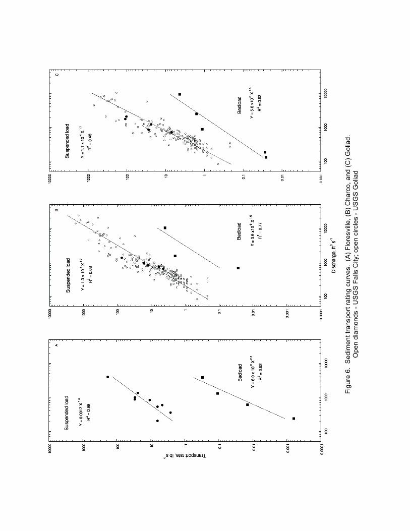
Most bedload consists of sand-sized sediment, although a small portion of relatively fine gravel is mobilized at all sites (Figure 7). There is a tendency for the bedload median diameter to decrease with increasing flow, which may reflect changes associated with bedform migration and/or the difficulty of capturing coarser grains using a portable

10

Figu

re 6

. S

edim

ent t

rans

port

ratin

g cu

rves

. (A

) Flo

resv

ille, (

B) C

harc

o, a

nd (C

) Gol

iad.

O

pen

diam

onds

- U

SGS

Fal

ls C

ity; o

pen

circ

les

- US

GS

Gol

iad

bedload sampler. In any case, the median diameter of bedload differs by less than 0.0061 in. at all sites.

2.4.1 Floodplain Accretion Depth In the Floresville reach, the January flood deposited 0.088 ft of sediment within 56 ft of the right bank edge in cross section 6. Given the proximity of a bridge pier to the cross section, this depth that may be enhanced through increased local flow resistance.

Figure 7. Grain size distributions for bedload. (a) Floresville, (b) Charco, and (c) Goliad. Distributions are identified by the discharge during sampling.

On the left bank, accretion occurred on the lower bank but not on the adjacent floodplain. Inspection of cross section 1 did not reveal any noticeable accretion that justified sampling by repeat survey but it is likely that a small amount of deposition occurred within the ground vegetation.

For the Charco reach, accretion near the bank-floodplain interface amounted to 0.0098 ft for the October flood. In the Goliad reach, accretion averaged 0.039 ± 0.02 ft and 0.034 ± 0.10 ft for the two sampling periods, respectively (Table 4).

Table 4. Accretion depths in the Goliad reach Cross Mean depth (ft) by sampling period

section 7/30/09-10/16/09 10/16/09-1/22/10 4 0.052 0.023 3 0.046 0.039 2 0.020 0.039

12

3 MODELING CHANNEL ADJUSTMENT The general modeling approach was to develop a hydraulic model for the three study reaches in the San Antonio River and select a sediment transport equation that permits the prediction of channel adjustment. Only 1-D hydraulic models were considered seriously for use because of the geomorphic processes under investigation, length of the study reaches, and available empirical data. Further, such models are relatively simple compared to 2-D and 3-D models and require the least amount of input data. Only models that are open source were considered to maximize cost effectiveness in evaluating instream flows.

The selected model HEC-RAS 4.0 (Hydrologic Engineering Centers River Analysis System) was developed by the Army Corps of Engineers to predict changes in channel shape and water surface profile given a set of flow and sediment transport boundary conditions (Warner et al., 2008). The model is among the most widely used programs by engineering consulting firms when designing channel restoration projects. This 1-D model can simulate steady or unsteady hydraulics over a mobile bed. It has the ability to model interaction and exchange between suspended load, bedload, and the active surface and subsurface portions of the riverbed.

3.1 Modeling Procedures One study reach, Floresville, was used for initial model setup to select the sediment transport function and conduct sensitivity analysis on model parameters. The Floresville reach was used as a test case because existing repeat cross-sectional survey of the channel was available so that an evaluation of model results against field measurements could be completed. Although the cross-sectional change extends over a longer time period than would be modeled in practice, the field observations provide an order of magnitude check on results.

3.1.1 Initial Model Setup for Sediment Transport Function Selection A number of modeling decisions, parameter values, and input data remained fixed across all of the runs using HEC-RAS (Table 5). Running RAS in this way allowed the sensitivity of the model to specific sediment transport equations to be assessed.

Using a 1 hour computational increment, setup runs used flow for the period between January 1, 2010 and March 31, 2010 because it encompasses part of the field program and includes three floods with a range in peak discharge (6650 ft3s-1 on January 16, 2010, 5320 ft3s-1 on February 4, 2010, and 2730 ft3s-1 on February 12, 2010) and two periods with extended, relatively low discharge (average around 250 ft3s-1 from January 1, 2010 to January 12, 2010 and 500 ft3s-1 from February 18, 2010 to April 10, 2010).

13

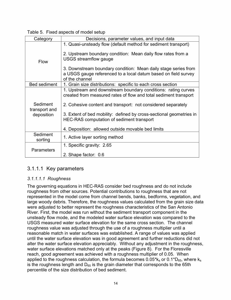
Table 5. Fixed aspects of model setup Category Decisions, parameter values, and input data

Flow

1. Quasi-unsteady flow (default method for sediment transport)

2. Upstream boundary condition: Mean daily flow rates from a USGS streamflow gauge

3. Downstream boundary condition: Mean daily stage series from a USGS gauge referenced to a local datum based on field survey of the channel

Bed sediment 1. Grain size distributions: specific to each cross section

Sediment transport and

deposition

1. Upstream and downstream boundary conditions: rating curves created from measured rates of flow and total sediment transport

2. Cohesive content and transport: not considered separately

3. Extent of bed mobility: defined by cross-sectional geometries in HEC-RAS computation of sediment transport

4. Deposition: allowed outside movable bed limits Sediment

sorting 1. Active layer sorting method

Parameters 1. Specific gravity: 2.65

2. Shape factor: 0.6

3.1.1.1 Key parameters

3.1.1.1.1 Roughness

The governing equations in HEC-RAS consider bed roughness and do not include roughness from other sources. Potential contributions to roughness that are not represented in the model come from channel bends, banks, bedforms, vegetation, and large woody debris. Therefore, the roughness values calculated from the grain size data were adjusted to better represent the roughness characteristics of the San Antonio River. First, the model was run without the sediment transport component in the unsteady flow mode, and the modeled water surface elevation was compared to the USGS measured water surface elevation for the same cross section. The channel roughness value was adjusted through the use of a roughness multiplier until a reasonable match in water surfaces was established. A range of values was applied until the water surface elevation was in good agreement and further reductions did not alter the water surface elevation appreciably. Without any adjustment in the roughness, water surface elevations matched only at the peaks (Figure 8). For the Floresville reach, good agreement was achieved with a roughness multiplier of 0.05. When applied to the roughness calculation, the formula becomes 0.05*ks or 0.1*D65, where ks is the roughness length and D65 is the grain diameter that corresponds to the 65th percentile of the size distribution of bed sediment.

14

3.1.1.1.2 Fall velocity The choices in HEC-RAS for computing fall velocities, and thus deposition of the finer sediments, include Toffaleti (1968) and Rubey (1933). Toffaletti created a table of fall velocities using a shape factor of 0.9 and specific gravity of 2.65. Fall velocities were measured over a range of temperatures (35°-90°F) for grain sizes from very fine sand to medium gravel (i.e., 0.0029 to 0.020 in.). The table is included in the HEC-RAS reference manual (p. 289), and the values are applied to the modeling within RAS to compute fall velocities. Rubey (1933) developed fall velocity equations by considering

Figure 8. Comparison of water surface elevations at the Floresville gauge. (A) roughness based on grain size of sediments and (B) roughness adjusted by multiplier of 0.05.

sediment properties in either Stokes law or an impact equation. Grain sizes ranged from silts to gravels, with a specific gravity of 2.65. Water temperature was fixed at 61°F.

Model results do not show sensitivity to the choice of fall velocity equation. The difference between the results based on the two methods was very small. The Toffaletti fall velocity method was used in all runs for consistency with the selected transport equation.

15

3.1.1.2 Sediment transport equations The choice of transport equation to predict sediment transport rates in any model is of paramount importance. Sediment transport formulae are developed under specific ranges of experimental conditions of flow hydraulics and boundary materials. In selecting the best available transport equation for the lower San Antonio River, the observed grain size distribution of the bed sediments was weighted heavily. In the Floresville reach, most bed sediment is in the sand range (Table 3). The reach averaged median diameter (D50) is 0.005 in., which is classified as very fine sand. The percentage of sediment in the gravel range (>0.08 in.) is between 0.02% and 10.9% with a reach average of 3.2%.

HEC-RAS offers seven formulae for sediment transport prediction. Some are designed for larger sediment (i.e., Meyer-Peter and Muller, Engelund-Hansen, and Yang equations) at high bedload transport rates (i.e., Wong and Parker modification of the Meyer-Peter and Muller equation) and thus inappropriate for the San Antonio River. Ackers-White and Laursen are total load equations, where the total sediment load is predicted as a single volume and not broken into individual grain size fractions. When fractional data are available, a multi-fractional transport equation can provide better results. From the HEC-RAS list, both the Toffaletti and Laursen equations were evaluated for their ability to replicate sediment transport rates in the Floresville reach.

3.1.1.2.1 Toffaletti

The Toffaletti equation (1968) calculates both bedload and suspended load, separating the suspended load distribution into four vertical zones in an attempt to replicate 2-D sediment transport. Sediment transport rates are calculated separately for each zone and then summed for a total transport rate. Toffaletti developed the equations for each zone from the calculated hydraulic parameters governing sediment movement and approximating the Rouse concentration profile through the water column. This is a fundamentally different approach than bedload transport equations (e.g., Wilcock-Crowe equation and Meyer-Peter and Muller equation) that calculate transport using the shear stresses acting on the sediments. A transport modeling approach based on the effects of flow hydraulics on the suspended and bed load sediment concentration makes the Toffaletti equation more appropriate in sand-bed channels. The equation has been applied successfully to large rivers, including the Mississippi, Arkansas, and Atchafalaya.

General transport equations for a single grain size in each of the zones (lower zone, middle zone, upper zone, and bed zone) are:

1+n !0.756 zv 1+n !0.756 z" R # $ % ! (2dm )

v

&11.24 ' g = MssL 1+ n ! 0.756 v z [1]

16

1+n !z 1+n !z0.244 z $ R % "$ R %

v

$ R % v #

& ! ' ( ) ( ) ( )*11.24 + &* 2.5 + *11.24 + '

gssM = M , -1+ nv ! z [2]

z 0.5 z 1+n !1.5 z0.244 " 1+nv!1.5 z #$ R % $ R % $ R % v

& R ! ' ( ) ( ) ( ) ( )*11.24 + * 2.5 + & * 2.5 + '

gssU = M , -1+ n !1.5 v z [3]

+n !0.756 zvgsb = M (2dm )1

[4]

0.756 z!nvM = 43.2 CL (1+ nv )VR [5]

g = g + g + g + gs ssL ssM ssU sb [6]

where gssL = suspended sediment transport in the lower zone (ton ft-1day-1), gssM = suspended sediment transport in the middle zone (ton ft-1day-1), gssU = suspended sediment transport in the upper zone (ton ft-1day-1), gsb = bed load sediment transport (ton ft-1day-1), gs = total sediment transport (ton ft-1day-1), M = sediment concentration parameter, CL = sediment concentration in the lower zone (lb ft3), R = hydraulic radius (ft), Dm = median grain diameter (ft), z = exponent describing the relationship between the sediment and hydraulic characteristics, and nv = temperature exponent. The zones are provided graphically in the HEC-RAS reference manual on p. 315. The Toffaletti equation is applicable to channels with grain sizes between 0.0025 in. and 0.16 in., median grain diameters between 0.018 in. and 0.036 in., flow velocities between 0.7 ft s-1 and 6.3 ft s-1, hydraulic radii between 0.07 ft and 57 ft, energy slopes between 0.00014 and 0.019, channel widths between 0.8 ft and 80 ft, and water temperatures between 40°F and 93°F.

3.1.1.2.2 Laursen (Copeland) The Laursen (1958) equation predicts of the total sediment load carried by the channel. It was derived from field and flume measurements using mean flow parameters. Sediment transport is quantified primarily as a function of channel hydraulics, specifically the flow velocity, flow depth, and energy slope. Sediment size is specified through a mean grain diameter and the fall velocity for that diameter. A modification by Copeland (1989) extended the applicability of the Laursen method to gravel sized sediments, and it is this modified form that is in RAS. The Laursen (Copeland) model may be applied to predict the total load of channels carrying sizes from 0.0043 in. to 1.1 in.

The method centers on the equation

17

7/6 $ d % $! ' % $ u %s o *Cm = 0.01 " ' ( &1( f ' (' ) D * ) ! c * ) # * [7]

where Cm = sediment discharge concentration (lb ft3), γ = specific weight of water (lb ft3), ds = mean grain size (ft), D = effective flow depth (ft), τc = critical shear stress (lb ft-2), τo’ = bed stress acting on bed grains (lb ft-2), u*= shear velocity (ft s-1), ω = fall velocity (ft s-1), and f = function of the ratio of the latter two variables as defined by a figure in Laursen (1958) that has been incorporated into HEC-RAS. Additionally, within RAS, the user establishes a maximum amount of scour that is possible in a channel reach, which is also known as a lower base the channel cannot erode below. The maximum level of scour is applicable primarily in channels with bedrock control or human-made structures.

3.1.1.3 Equation performance in the Floresville reach The choice of sediment transport equation was made by evaluating results from simulations in the Floresville reach and comparing them against known historical changes and associated sediment transport in the lower San Antonio River described in section 2.2.2.

3.1.1.3.1 Toffaletti The reach average change in channel invert elevation from the Toffaletti method was a reduction of 4.0 ft, indicating that over the 3 month period the channel bed degraded an average of 4.0 ft at its deepest point. The amount of erosion was variable at the different cross sections, ranging between 0.7 ft and 6.1 ft. Over a 24 hour period, the model predicts a maximum channel aggradation of 0.2 ft at the channel invert and maximum erosion of 5.9 ft. The resulting cumulative mass change in the bed is 28,949 tons of net sediment loss. The predicted rate from the RAS model is higher than the extrapolated rate from the FM775 cross-section (i.e., 11,307 tons). This suggests that the preliminary model overestimates bed adjustment based on the available empirical data.

3.1.1.3.2 Laursen (Copeland) For the Floresville reach, the maximum erosion level limit was set to 180 ft simply to provide a large value so that the model would run without any influence from the scour limit. The bed eroded steadily to this maximum during the flow simulation. There was no difference in the results with either the Toffaletti or Rubey fall velocity equations. Overall, for the flow rates evaluated, the observed grain size and cross-sectional morphology, and imposed scour limit, the Laursen (Copeland) transport model did not provide realistic results.

3.1.1.3.3 Transport equation selection The three reaches in the Lower San Antonio River were modeled using the Toffaletti transport method. The resulting pattern of sediment mass movement provided the best preliminary match of flux rates in and out of the cross sections. Although the total

18

amount of erosion predicted by the Toffaletti method is relatively large, the pattern and direction of channel change are more realistic than results from the Laursen equation. Predictions from a sediment transport function as a mass capacity can be compared to those estimated from empirical transport rating curves to gain a general assessment of the performance of the transport function. In doing so, it must be kept in mind that errors will be present in both and that prediction of sediment transport rates is unlikely to be exact given well known issues with the use of transport equations.

3.1.2 Refined Model Setup for Reach Study Simulations Based on preliminary simulations, three changes were incorporated into the modeling procedure as follows.

(i) The length of channel modeled was extended beyond the study reaches by adding a cross section at both the upstream and downstream ends. The extension cross sections were the same morphology as the nearest measured cross section and separated by a similar distance. This strategy helped to reduce the influence of imposed boundary conditions on the channel adjustments in the actual study reaches and provided more realistic results. The extension cross sections were not considered in the analysis of model output.

(ii) The streamflow record used for simulation was extended over approximately two years (January 1, 2009 - March 1, 2011) to provide a longer temporal view on transport rates and channel adjustment.

(iii) Calibration procedures were refined to improve modeling results by increasing the similarity between observed and modeled water surface elevations. First, calibration of modeled water surface elevations to those observed at the USGS gauges was performed using the RAS model with steady flow. The bed roughness factor was calculated within the RAS program but it was modified by using a roughness multiplier to improve the water surface calibration. This strategy was followed until the modeled water surface showed an acceptable similarity to the observed elevations at selected flow rates. Similarity was tested over at least seven flow rates that are representative of those in the study reaches.

Second, the model was run under unsteady flow conditions and results compared to the flow series. Testing a range of boundary conditions revealed that the best fit occurred with a flow hydrograph for the upstream boundary condition and a stage hydrograph for the downstream boundary condition. Further, flow roughness factors were added to the calibration, which permitted the bed roughness factor to change as a function of the flow rate and resulted in improved calibration at both low and high flow rates. After the calibration steps of adjusting the bed roughness factor by a roughness multiplier and applying flow roughness factors to the bed roughness factor under the selected flow rates, the model was run as a quasi-steady state model with sediment transport.

Comparison between water surface elevations for the USGS flow series and model

19

output revealed a consistent lag of 24 hours, which suggests a possible error in time assignment in HEC-RAS that could not be resolved. Results for the study reach models are presented with this 24-hour lag eliminated through a shift in the USGS surface elevations, given that the timing error does not affect the degree to which the model simulates the given the flow series.

3.2 Reach Models and Simulation Results

3.2.1 Floresville Reach

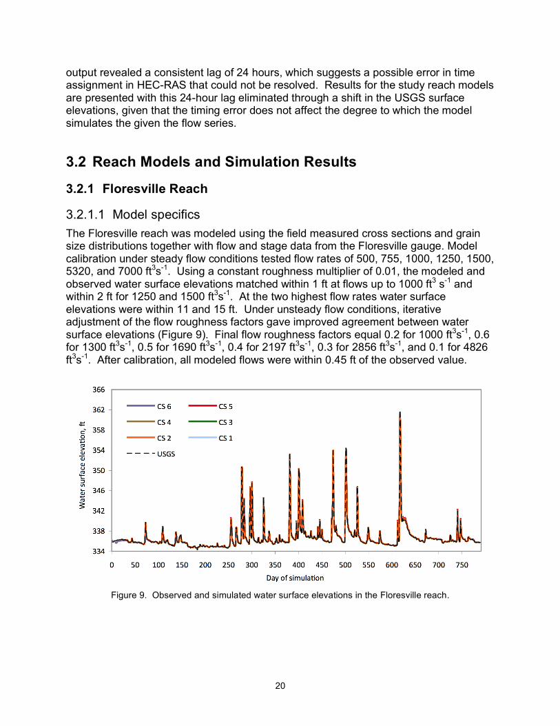
3.2.1.1 Model specifics The Floresville reach was modeled using the field measured cross sections and grain size distributions together with flow and stage data from the Floresville gauge. Model calibration under steady flow conditions tested flow rates of 500, 755, 1000, 1250, 1500, 5320, and 7000 ft3s-1. Using a constant roughness multiplier of 0.01, the modeled and observed water surface elevations matched within 1 ft at flows up to 1000 ft3 s-1 and within 2 ft for 1250 and 1500 ft3s-1. At the two highest flow rates water surface elevations were within 11 and 15 ft. Under unsteady flow conditions, iterative adjustment of the flow roughness factors gave improved agreement between water surface elevations (Figure 9). Final flow roughness factors equal 0.2 for 1000 ft3s-1, 0.6 for 1300 ft3s-1, 0.5 for 1690 ft3s-1, 0.4 for 2197 ft3s-1, 0.3 for 2856 ft3s-1, and 0.1 for 4826 ft3s-1. After calibration, all modeled flows were within 0.45 ft of the observed value.

Figure 9. Observed and simulated water surface elevations in the Floresville reach.

20

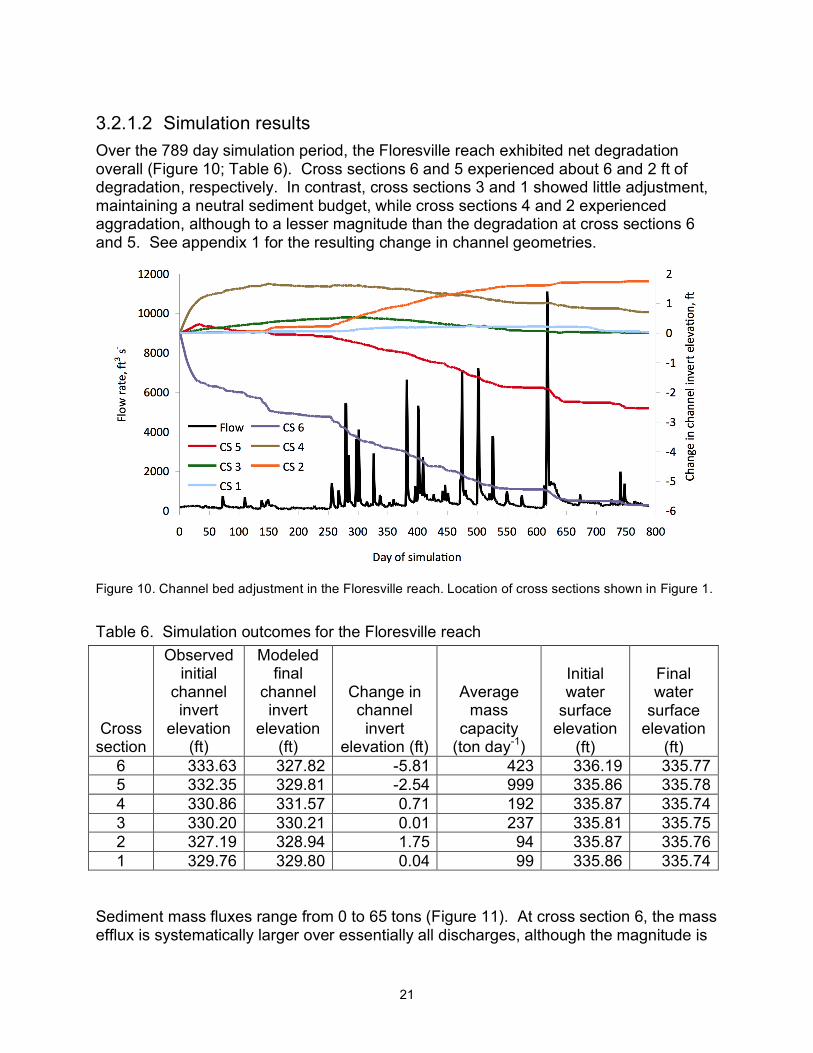
3.2.1.2 Simulation results Over the 789 day simulation period, the Floresville reach exhibited net degradation overall (Figure 10; Table 6). Cross sections 6 and 5 experienced about 6 and 2 ft of degradation, respectively. In contrast, cross sections 3 and 1 showed little adjustment, maintaining a neutral sediment budget, while cross sections 4 and 2 experienced aggradation, although to a lesser magnitude than the degradation at cross sections 6 and 5. See appendix 1 for the resulting change in channel geometries.

Figure 10. Channel bed adjustment in the Floresville reach. Location of cross sections shown in Figure 1.

Table 6. Simulation outcomes for the Floresville reach

Cross section

Observed initial

channel invert

elevation (ft)

Modeled final

channel invert

elevation (ft)

Change in channel invert

elevation (ft)

Average mass

capacity (ton day-1)

Initial water

surface elevation

(ft)

Final water

surface elevation

(ft) 6 333.63 327.82 -5.81 423 336.19 335.77 5 332.35 329.81 -2.54 999 335.86 335.78 4 330.86 331.57 0.71 192 335.87 335.74 3 330.20 330.21 0.01 237 335.81 335.75 2 327.19 328.94 1.75 94 335.87 335.76 1 329.76 329.80 0.04 99 335.86 335.74

Sediment mass fluxes range from 0 to 65 tons (Figure 11). At cross section 6, the mass efflux is systematically larger over essentially all discharges, although the magnitude is

21

not especially large. Influxes and effluxes at cross sections 3 and 1 are very similar, while at cross section 5 the similarity deviates notably only in the 20 to 30 ton range. The remaining two cross sections show disparities between influx and efflux masses that increase slightly as the flux increases. At cross section 4, some influxes less than 20 tons have substantially smaller effluxes. The total mass capacity for the simulation period of January 1, 2009 to February 28, 2011 amounts to 8.8 x 104 tons at cross section 1, which is less than the 4.0 x 105 tons derived from the empirical total sediment load rating curve. Inspection of the predicted and observed flow rates and sediment loads on a daily basis suggests that the underestimation derives from under-prediction at nearly all flow rates. Under-prediction is especially notable at the lower and upper discharge ranges, with departures at the highest flows particularly pronounced (two to three orders of magnitude).

Figure 11. Sediment mass fluxes in the Floresville reach. (A) CS 6, (B) CS 5, (C) CS 4, (D) CS 3, (E) CS 2, and (F) CS 1

3.2.2 Charco Reach

3.2.2.1 Model specifics The Charco reach was modeled using the field measured cross sections and grain size distributions together with flow and stage data from the Goliad gauge adjusted for differences in contributing area and land elevation, respectively. Model calibration

22

under steady flow conditions tested flow rates of 500, 810, 1012, 1247, 2365, 4989, and 6958 ft3s-1. A constant bed roughness multiplier of 0.01 provided a match of water surface elevations to within 1 ft at all selected flow rates. During unsteady flow calibration a final set of flow roughness factors were identified for five flow rates: 0.1 for

-1 -1500 ft3s-1, 3.5 for 1012 ft3s , 0.01 for 2365 ft3s , 2.2 for 4989 ft3s-1, and 0.01 for 6958 ft3s-1. Greater discrepancies remained between the modeled and observed water surface elevations in this study reach compared to both Floresville and Goliad. Modeled water surface elevations at the upstream cross sections are from 4 to 7.7 ft larger than those for the adjusted USGS flow series, while those at the downstream cross sections are better matched, with differences between 0.8 and 2.1 ft (Figure 12).

Figure 12. Observed and simulated water surface elevations in the Charco reach.

3.2.2.2 Simulation results Over the simulation period, the Charco reach exhibits net degradation overall (Figure 13; Table 7). The bed elevation decreases by about 2 ft at cross sections 5 and 2 but only around 0.4 ft at cross sections 4 and 3. Aggradation that occurs at cross section 1 amounts to 1.4 ft. See appendix 2 for the resulting change in channel geometries.

23

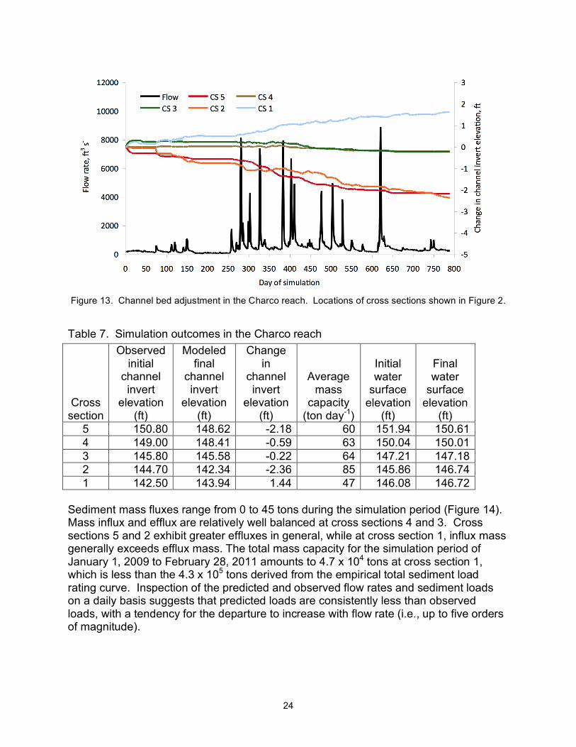
Figure 13. Channel bed adjustment in the Charco reach. Locations of cross sections shown in Figure 2.

Table 7. Simulation outcomes in the Charco reach

Cross section

Observed initial

channel invert

elevation (ft)

Modeled final

channel invert

elevation (ft)

Change in

channel invert

elevation (ft)

Average mass

capacity (ton day-1)

Initial water

surface elevation

(ft)

Final water

surface elevation

(ft) 5 150.80 148.62 -2.18 60 151.94 150.61 4 149.00 148.41 -0.59 63 150.04 150.01 3 145.80 145.58 -0.22 64 147.21 147.18 2 144.70 142.34 -2.36 85 145.86 146.74 1 142.50 143.94 1.44 47 146.08 146.72

Sediment mass fluxes range from 0 to 45 tons during the simulation period (Figure 14). Mass influx and efflux are relatively well balanced at cross sections 4 and 3. Cross sections 5 and 2 exhibit greater effluxes in general, while at cross section 1, influx mass generally exceeds efflux mass. The total mass capacity for the simulation period of January 1, 2009 to February 28, 2011 amounts to 4.7 x 104 tons at cross section 1, which is less than the 4.3 x 105 tons derived from the empirical total sediment load rating curve. Inspection of the predicted and observed flow rates and sediment loads on a daily basis suggests that predicted loads are consistently less than observed loads, with a tendency for the departure to increase with flow rate (i.e., up to five orders of magnitude).

24

Figure 14. Sediment mass fluxes in the Charco reach. (A) CS 5, (B) CS 4, (C) CS 3, (D) CS 2, and (E) CS 1.

3.2.3 Goliad Reach

3.2.3.1 Model specifics The Goliad reach was modeled using the field measured cross sections and grain size distributions together with flow and stage data from the Goliad gauge. Model calibration under steady flow conditions tested flows at 500, 765, 1000, 1300, 2000, 3500, 6000, 9000, and 11000 ft3s-1. Using a final bed roughness multiplier of 0.001, the modeled and observed water surface elevations differed by between 0.3 and 1.3 ft. The best match was at the low flows and the worst was for the mid range flows of 2000 and 3500 ft3s-1. During unsteady flow calibration iterative adjustment of the flow roughness factor did not have an appreciable effect on the calibration beyond a single adjustment of 0.1 for flows between 90 and 100 ft3s-1. The final modeled water surface elevations differed from those observed by between 0.009 ft and 1.2 ft, and all but 10 days had modeled water surface elevations within 0.3 ft of the observed values (Figure 15).

25

Figure 15. Observed and simulated water surface elevations in the Goliad reach

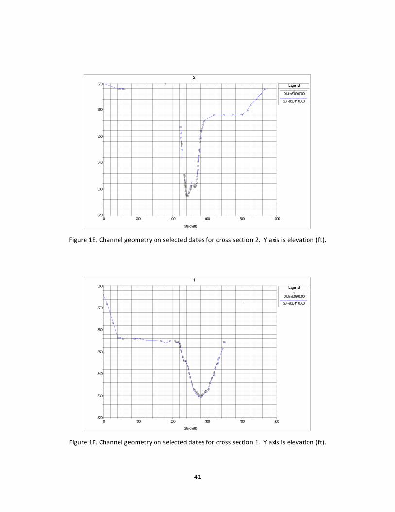
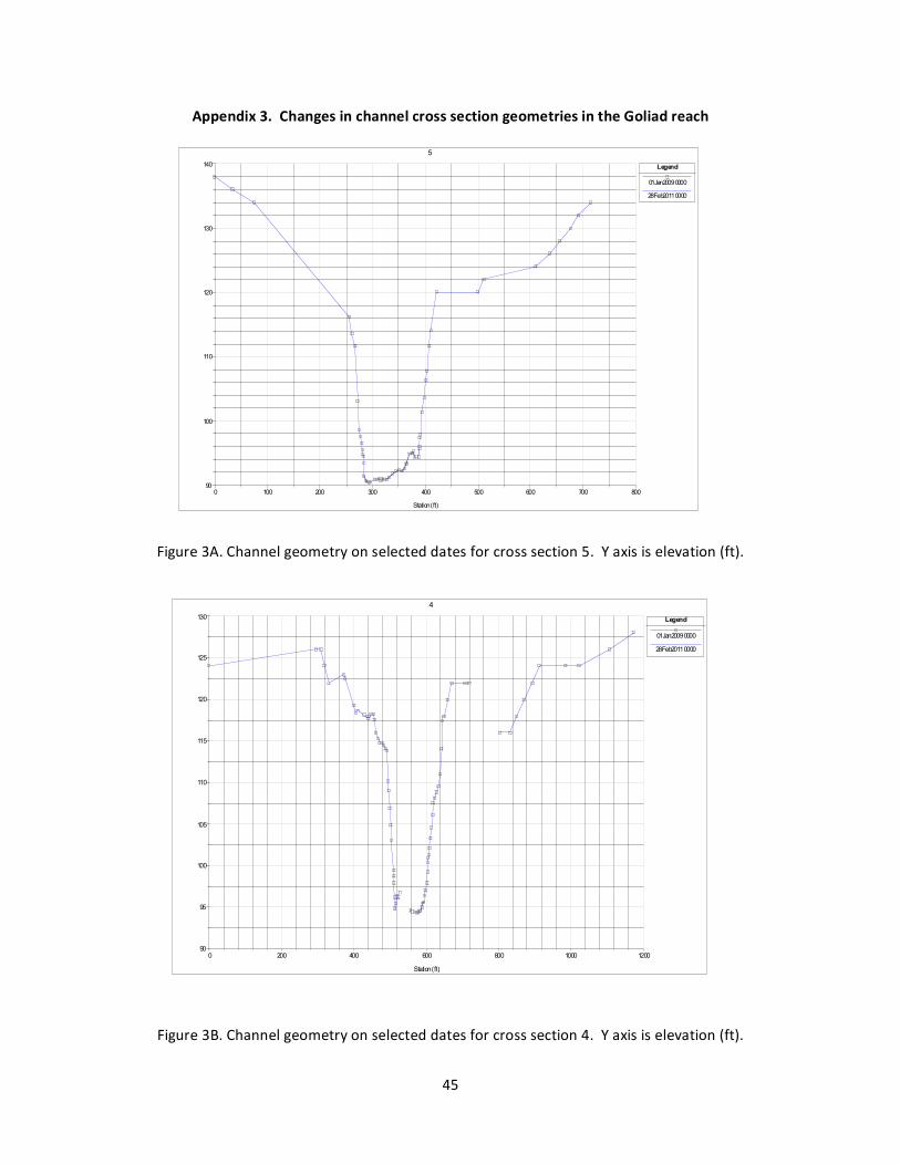
3.2.3.2 Simulation results Over the simulation period, the bed elevation of the Goliad reach is essentially stable (Figure 16; Table 8). Very minor degradation occurs at cross sections 5 and 4, while very minor aggradation is experienced at cross sections 3, 2, and 1. See appendix 3 for the resulting change in channel geometries.

Figure 16. Channel bed adjustment in the Goliad reach. Note expanded elevation scale relative to that in Figures 10 and 13. Locations of cross sections shown in Figure 3.

26

Table 8. Simulation outcomes in the Goliad reach

Cross section

Observed initial

channel invert

elevation (ft)

Modeled final

channel invert

elevation (ft)

Change in channel invert

elevation (ft)

Average mass

capacity (ton day-1)

Initial water

surface elevation

(ft)

Final water

surface elevation

(ft) 5 90.49 90.44 -0.05 0.58 96.35 96.65 4 94.33 94.13 -0.20 2.26 96.17 96.50 3 90.68 90.76 0.08 2.15 96.27 96.58 2 92.59 92.66 0.07 0.18 96.27 96.58 1 85.63 85.64 0.01 0.15 96.28 96.59

Sediment mass fluxes range from 0 to 5 tons (Figure 17). Paired influxes and effluxes are similar at cross section 1. At cross sections 5 and 4, effluxes generally exceed influxes, while at cross sections 3 and 2, influxes generally exceed effluxes. The total mass capacity for the simulation period of January 1, 2009 to February 28, 2011 amounts to 2.7 x 104 tons at cross section 2, which is less than the 6.5 x 105 tons derived from the empirical total sediment load rating curve. Inspection of the predicted and observed flow rates and sediment load on a daily basis suggests that flow rates larger than 2000 ft3 s-1 are under-predicted by about two orders of magnitude. Additionally, predictions at low flow rates (<200 ft3 s-1) are poorly matched.

Figure 17. Sediment mass fluxes in the Goliad reach. (A) CS 5, (B) CS 4, (C) CS 3, (D) CS 2, and (E) CS 1. Note expanded axes compared to the Floresville and Charco results.

27

3.2.3.3 Model performance In absolute terms, the observed change in bed elevation averaged 1.7 ft, while the modeled change amounted to a degradation of the channel invert of 0.014 ft, indicating that the model underpredicts the overall magnitude of change in the reach (Table 9). Additionally, the direction of change is not always predicted well, suggesting that changes at specific cross sections may be misleading based on the limited verification data.

Table 9. Observed and modeled bed elevations in the Goliad reach1

Cross section Time period

Observed change in bed

elevation, ft

Modeled change in bed

elevation, ft 4 7/29-09 - 2/10/10 1.6 -0.014 3 8/8/09 - 2/10/10 0.6 -0.014 2 7/25/09 - 2/10/10 -2.8 -0.014

1 Positive numbers indicate aggradation and negative numbers indicate degradation

4 MODELING FLOODPLAIN ACCRETION Modeling employed part of the floodplain sedimentation model described in Nicholas et al. (2006). The general approach develops predictive relations for floodplain accretion based on excess discharge, an easily determined flow that is the difference between the total rate and bankfull rate. At a given cross section, flow conveyed on the floodplain is determined for a given water surface elevation from

S W /2 1.67 Q = 2 H dx F !n 0 [8]

where QF = flow rate on the floodplain (ft3s-1), S = slope (ft ft-1), n = Manning’s roughness factor for the floodplain, and W = cross-sectional width of the floodplain and H = overbank flow depth (ft), both at a given water surface elevation (ft). The accretion rate depends on the flow conditions on the floodplain and the concentration of sediment in suspension and is given by

WHC D = V !" [9]

where D = sedimentation rate per unit valley length (lb ft-1s-1), C = concentration of suspended sediment in the flow (lb ft-3), V = flow velocity on the floodplain (ft s-1), α = calibration parameter found by Nicholas et al. to be approximately equal to 1, and β = parameter to account for the mechanism by which sediment is deposited on the

28

!

!

!

floodplain. When sediment trapping by vegetation plays a role β can range from 1 to 2. The relation for accretion is established in the form of

D = " (Q # Qbf )$

[10]

where Q = flow rate in the cross section (ft3s-1), Qbf = bankfull flow rate for the cross section (ft3s-1), and Γ and Λ = empirically fitted parameters.

In this study, the accretion rate was derived for each cross section by modifying equation [10] to

)$ d = " a(Q # Qbf [11]

where d = floodplain accretion rate (ft min-1) and " a = ) +*

1 $#" & (' %s

where ρs = sediment

density and φ = sediment porosity. This modification permitted cross-sectional models to be calibrated based on available field observations of floodplain accretion and the overbank flood hydrographs. A reach-based model of floodplain accretion was constructed by pooling individual cross-sectional results.

4.1 Modeling Procedures

4.1.1 Floodplain Flow Conditions Rating curves for overbank flow were developed for all cross sections in the study reaches. First, a relation between the flow rate and stage height was constructed using approximately four years (January 2006 to March 2011) of USGS streamflow data to capture a range of overbank flows. For the Charco reach, where flow gauging information is not available in the reach, Goliad flow data were adjusted downward by 19% based on the contributing areas of the two locations. Stage height was converted to water surface elevation (WSEL) at each cross section using HEC-RAS modeling results. The WSEL at bankfull condition was defined for each cross section using field observations and major breaks in slope in the channel cross-sectional configuration. Bankfull flow was then determined from the flow rate-WSEL power function and this discharge was used to truncate the flow rating curve to represent only overbank flows.

Overbank flows were characterized in terms of flow width, depth, and velocity for input into the accretion model (equation 9). Based on the channel cross sections and flow-rate WSEL power functions, the full width of flow inundation was determined for a range of overbank flows from which the bankfull channel width was subtracted to leave the inundated floodplain width relative to both sides of the channel. The corresponding flow depth over the floodplain area was estimated by calculating the difference between the elevations of the water surface at bankfull and the given overbank flow and dividing by 2 to represent the mean flow depth. This assumes a simplified cross section and use of equation [8] but the known floodplain topography indicates this is a reasonable

29

!

assumption. Flow velocity over the floodplain was determined using Manning’s equation, given as

R0.67S0.5

V = 1.49 [12] n f

where R = hydraulic radius (ft), S = energy slope (ft ft-1), and nf = floodplain roughness coefficient. The hydraulic radius was calculated based on derived flow depths and widths for the floodplain area, while the roughness value was set to that used in the calibration of the RAS model. The slope was based on a reach-based estimate derived from water surface elevations near a bankfull condition.

4.1.2 Floodplain Accretion For each cross section, D was calculated for a range of overbank flows using equation [9]. C was quantified by adjusting the suspended sediment concentration rating curve developed from empirical observations to better represent likely concentrations over the floodplain. This adjustment was guided by suspended sediment sampling at Goliad during an overbank flow. Samples collected from the upper portion of the water column over the channel and from the inundated floodplain suggest that concentrations are only about half of that predicted by the rating curve for the same discharge. Thus, concentration rating curves for the three subreaches were adjusted downward by 0.5. β was set equal to 1 to reflect the presence of riparian vegetation in the study reaches, while α was set initially equal to 1 following Nicholas et al. (2006). Sensitivity analysis for parameters α and β suggested that α exerts a larger impact on results.

Computed D values were adjusted for sediment density and porosity and then regressed against excess overbank flow (Q-Qbf) to empirically determine the coefficients Γa and Λ in equation [11]. Local grain size characteristics of floodplain sediment were used to estimate typical sediment densities and porosities. Sediment density was computed as a weighted mean based on the proportion of major grain size classes. Porosities were estimated based on the median grain size diameter using Komura's (1961) equation for river sediment.

Where possible, accretion models were calibrated by adjusting α in equation [9] until the predicted accretion depth matched the measured accretion depth. Predicted accretion depths were determined by using the predicted relation for the 15 minute flow series that represented overbank conditions at each calibration cross section. Reach specific details of these adjustments are contained in the next section.

Once the relations for accretion rate were finalized for each cross section, the predicted values of d for the range of excess flow considered in all cross sections for a given study reach were pooled and regressed to construct a reach-based model of floodplain accretion. Building a reach model in this way incorporates the local variability that can be found within a study reach.

30

4.2 Reach Accretion Models

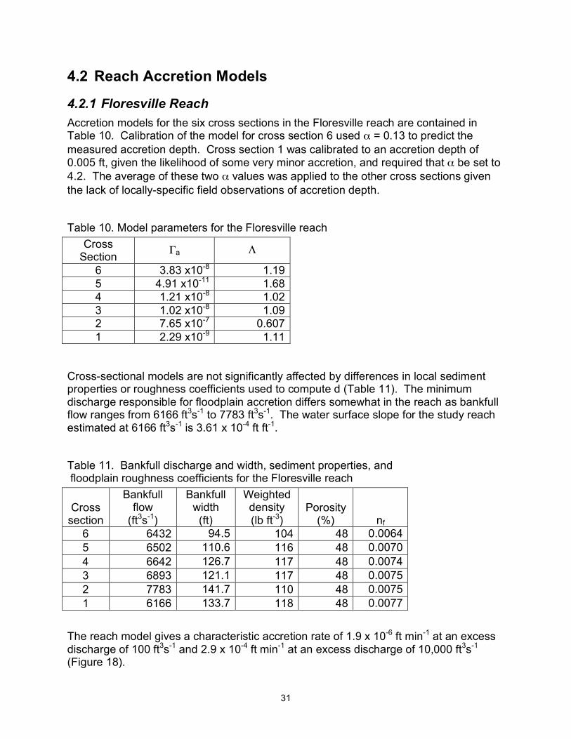
4.2.1 Floresville Reach Accretion models for the six cross sections in the Floresville reach are contained in Table 10. Calibration of the model for cross section 6 used α = 0.13 to predict the measured accretion depth. Cross section 1 was calibrated to an accretion depth of 0.005 ft, given the likelihood of some very minor accretion, and required that α be set to 4.2. The average of these two α values was applied to the other cross sections given the lack of locally-specific field observations of accretion depth.

Table 10. Model parameters for the Floresville reach Cross

Section Γa Λ

6 3.83 x10-8 1.19 5 4.91 x10-11 1.68 4 1.21 x10-8 1.02 3 1.02 x10-8 1.09 2 7.65 x10-7 0.607 1 2.29 x10-9 1.11

Cross-sectional models are not significantly affected by differences in local sediment properties or roughness coefficients used to compute d (Table 11). The minimum discharge responsible for floodplain accretion differs somewhat in the reach as bankfull flow ranges from 6166 ft3s-1 to 7783 ft3s-1. The water surface slope for the study reach estimated at 6166 ft3s-1 is 3.61 x 10-4 ft ft-1.

Table 11. Bankfull discharge and width, sediment properties, and floodplain roughness coefficients for the Floresville reach

Cross section

Bankfull flow

(ft3s -1)

Bankfull width (ft)

Weighted density (lb ft-3)

Porosity (%) nf

6 6432 94.5 104 48 0.0064 5 6502 110.6 116 48 0.0070 4 6642 126.7 117 48 0.0074 3 6893 121.1 117 48 0.0075 2 7783 141.7 110 48 0.0075 1 6166 133.7 118 48 0.0077

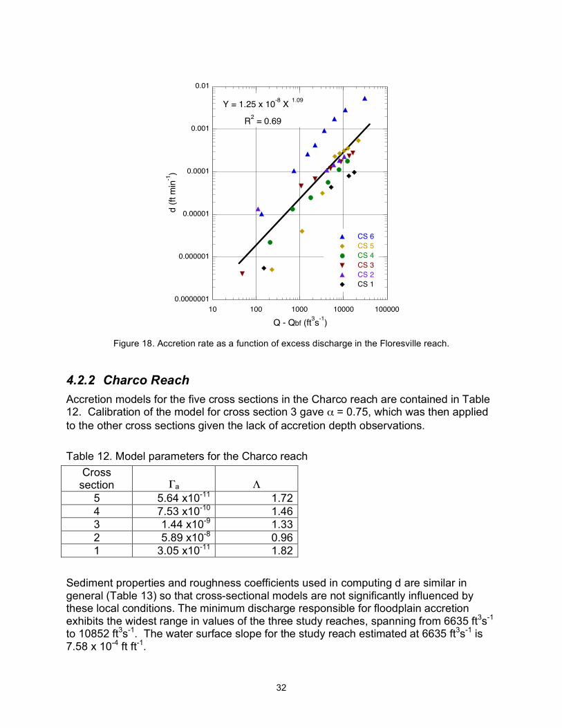
The reach model gives a characteristic accretion rate of 1.9 x 10-6 ft min-1 at an excess discharge of 100 ft3s-1 and 2.9 x 10-4 ft min-1 at an excess discharge of 10,000 ft3s-1

(Figure 18).

31

0.0000001

0.000001

0.00001

0.0001

0.001

0.01

CS 6 CS 5 CS 4 CS 3 CS 2 CS 1

d (ft

min

-1 )

Y = 1.25 x 10-8 X 1.09

R2 = 0.69

10 100 1000 10000 100000 -1)Q - Qbf (ft3s

Figure 18. Accretion rate as a function of excess discharge in the Floresville reach.

4.2.2 Charco Reach Accretion models for the five cross sections in the Charco reach are contained in Table 12. Calibration of the model for cross section 3 gave α = 0.75, which was then applied to the other cross sections given the lack of accretion depth observations.

Table 12. Model parameters for the Charco reach Cross

section Γa Λ 5 5.64 x10-11 1.72 4 7.53 x10-10 1.46 3 1.44 x10-9 1.33 2 5.89 x10-8 0.96 1 3.05 x10-11 1.82

Sediment properties and roughness coefficients used in computing d are similar in general (Table 13) so that cross-sectional models are not significantly influenced by these local conditions. The minimum discharge responsible for floodplain accretion exhibits the widest range in values of the three study reaches, spanning from 6635 ft3s-1

to 10852 ft3s-1. The water surface slope for the study reach estimated at 6635 ft3s-1 is 7.58 x 10-4 ft ft-1.

32

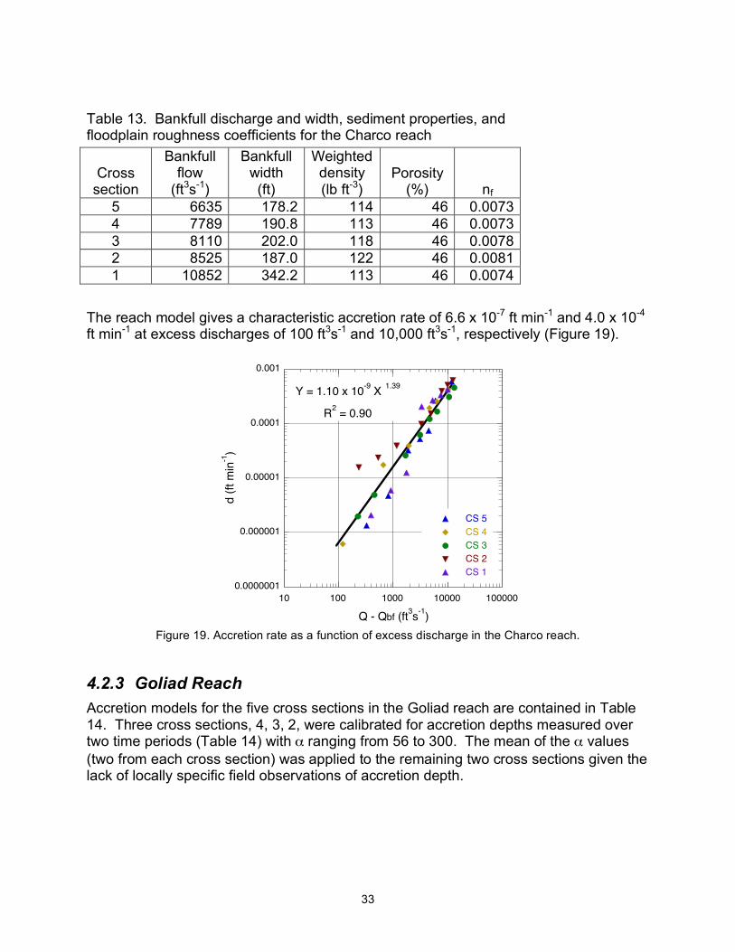
Table 13. Bankfull discharge and width, sediment properties, and floodplain roughness coefficients for the Charco reach

Cross section

Bankfull flow

(ft3s -1)

Bankfull width (ft)

Weighted density (lb ft-3)

Porosity (%) nf

5 6635 178.2 114 46 0.0073 4 7789 190.8 113 46 0.0073 3 8110 202.0 118 46 0.0078 2 8525 187.0 122 46 0.0081 1 10852 342.2 113 46 0.0074

The reach model gives a characteristic accretion rate of 6.6 x 10-7 ft min-1 and 4.0 x 10-4

ft min-1 at excess discharges of 100 ft3s-1 and 10,000 ft3s-1, respectively (Figure 19).

0.0000001

0.000001

0.00001

0.0001

0.001

CS 5 CS 4 CS 3 CS 2 CS 1

d (ft

min

-1)

Y = 1.10 x 10-9 X 1.39

R2 = 0.90

10 100 1000 10000 100000 -1)Q - Qbf (ft3s

Figure 19. Accretion rate as a function of excess discharge in the Charco reach.

4.2.3 Goliad Reach Accretion models for the five cross sections in the Goliad reach are contained in Table 14. Three cross sections, 4, 3, 2, were calibrated for accretion depths measured over two time periods (Table 14) with α ranging from 56 to 300. The mean of the α values (two from each cross section) was applied to the remaining two cross sections given the lack of locally specific field observations of accretion depth.

33

Table 14. Model parameters for the Goliad reach Cross section Γa Λ

5 1.16 x10-11 1.62 4 period 1 4.45 x10-11 1.56 4 period 2 1.38 x10-11 1.56 3 period 1 1.10 x10-10 1.52 3 period 2 8.19 x10-11 1.52 2 period 1 1.61 x10-9 1.02 2 period 2 2.09 x10-9 1.02

1 1.90 x10-7 0.461

Cross-sectional models are not significantly affected by differences in local sediment properties used in computing d, but roughness coefficients exhibit the widest range of the three study reaches and may exert some influence (Table 15). The minimum discharge responsible for floodplain accretion ranges from 5863 ft3s-1 to 9112 ft3s-1. The water surface slope for the study reach estimated at 6635 ft3s-1 is 5.68 x 10-6 ft ft-1.

Table 15. Bankfull discharge and width, sediment properties, and floodplain roughness coefficients for the Goliad reach

Cross section

Bankfull flow

(ft3s -1)

Bankfull width (ft)

Weighted density, (lb ft-3)

Porosity (%) nf

5 9217 158.1 120 51 0.0072 4 5863 151.5 122 51 0.0072 3 7415 157.1 115 51 0.0075 2 6114 146.3 103 51 0.0057 1 9112 161.4 100 51 0.0054

The reach model gives a characteristic accretion rate of 9.6 x 10-8 ft min-1 at an excess discharge of 100 ft3s-1 and 4.4 x 10-5 ft min-1 at an excess discharge of 10,000 ft3s-1

(Figure 20).

34

0.001

0.0001

0.00001

0.000001

0.0000001

0.00000001

CS 5 CS 4 period 1CS 4 period 2CS 3 period 1CS 3 period 2CS 2 period 1CS 2 period 2CS 1

Y = 2.10 x 10-10 X 1.33

R2 = 0.83

d (ft

min

-1)

100 1000 10000 100000 -1)Q - Qbf (ft3s

Figure 20. Accretion rate as a function of excess discharge in the Goliad reach.

5 CONCLUSION The HEC-RAS models developed provide initial models for predicting channel adjustment to a flow series in three distinct reaches in the lower San Antonio River. The reach models for the three study reaches are calibrated based on a fairly extensive field data set compared to other modeling projects. Nonetheless, the verification of the Goliad reach model suggests that the models, as developed so far, can provide only an initial assessment of possible channel adjustment. Given the uncertainties inherent in all sediment transport equations and the issues discussed below, HEC-RAS model output should be interpreted only as a general indication of the possible adjustment to the channel. The specific output of the models should not be regarded as exact measures of aggradation or degradation for the simulated flow series.

Like most hydraulic models, HEC-RAS models are highly dependent on key river observations. For example, channel cross-sectional information is used to create the channel geometry, and to obtain the necessary level of accuracy, some type of field surveying is necessary. An informed choice of sediment transport equation requires grain size information about the channel bed and sediment load, for which field samples are required. Inadequate efforts to characterize the channel, flow hydraulics, and the sediment regime of a river undermine the level of certainty in model output. Further work in acquiring field observations could improve model calibration. First, increasing the number of channel cross sections in the study reaches should improve the ability of the models to capture channel adjustment (Wallerstein, 2006). At present the cross

35

sections do not systematically characterize all areas of the channel morphology, which can exhibit different trends of local aggradation and degradation. More closely spaced cross sections would help capture locally variable sediment fluxes through the modeled reach. Related to this, documenting changes to the channel, particularly the bed elevation, would be helpful in verifying the ability of the reach models to predict channel adjustment. Second, water surface slopes derived from the HEC-RAS modeling have not been field verified nor have independent estimates of channel and floodplain roughness that explicitly take into account all roughness factors (e.g., large woody debris and vegetation on banks and the floodplain) been made. Efforts in both areas should improve the calibration of the models and hence their usefulness. Third, it may be beneficial to re-evaluate the selection of the sediment transport equation once more field observations are available to calibrate the models. It may be that the transport functions available in HEC-RAS are not sufficiently varied to provide the best possible one for modeling channel adjustment in the San Antonio River. Related to this, confidence in the empirical sediment transport rating curves could be improved through further collection of transport observations at higher flow rates. When adequately calibrated to a specific river, HEC-RAS modeling should be an effective tool for aiding management decisions.

The reach accretion models provide initial models for predicting floodplain accretion to a first order approximation. Key advantages of the models include the straightforward, simple computation and incorporation of accretion variability that arises over longer study reaches because flow and channel characteristics vary. Given the limited calibration of the models in terms of overbank flow events and observed accretion depths, the accretion model output should be interpreted only as a general indication of the possible magnitude of floodplain accretion.

To improve the accuracy of the accretion models more thorough calibration using field observations is required. First, observations of accretion depth were limited due to the number of overbank flows that occurred during the field program and number of channel cross sections that could be directly accessed over land. Repeated survey of the channel cross sections, or other measurement approaches that quantify accretion depth (e.g., sediment traps), would permit all cross-sectional models to be calibrated using locally-derived values of α in computing D, which has a significant effect on predicted accretion depths. Second, the computation of D is also influenced by the flow velocity estimated for the floodplain through the Manning's equation. However, water surface slopes derived from the HEC-RAS modeling have not been field verified nor have independent estimates of floodplain roughness that explicitly take into account riparian vegetation been made, both of which should help improve the accuracy of the flow velocity estimates and the resulting D values. Overbank flow velocity could also be directly measured to improve this aspect of the model.

In regard to the conceptual model underlying the accretion model, accretion is assumed to occur continuously during an overbank flow. While sediment trapping by vegetation was observed in the field, the extent to which sediment settling is restricted by flow velocity and associated turbulence is not strictly known. Moreover, the relative

36

importance of the two processes has not been established for the lower San Antonio River. A more sophisticated understanding of the mechanisms that cause sediment deposition (i.e., settling versus trapping) could improve the model calibration through parameter β, while a correction for the effective time over which settling occurs during overbank flows would likely improve model predictions. The latter would require an understanding of the concentration and grain size of suspended sediment in overbank flows.

Overall, the field observations and results of the reach models suggest that the geomorphic response to a given prescribed in-stream flow will not occur uniformly in the lower San Antonio River. River characteristics are sufficiently different to generate a range in responses. This variability in geomorphic response needs to be accounted for in river management decisions.

6 REFERENCES CITED Cawthon, T. and J.C. Curran, 2008. Channel Change on the San Antonio River, Texas.

Report for Project 0604830638. Texas Water Development Board In-Stream Flow Program. 52 pp.

Copeland, R.R. and W.A. Thomas, 1989. Corte Madera Creek Sedimentation Study. Numerical Model Investigation. US Army Engineer Waterways Experiment Station, Vicksburg, MS. TR-HL-89-6.

Engel, F.L. and J.C. Curran, 2008. Geomorphic Classification of the Lower San Antonio River, Texas. Report for Project 0604830637. Texas Water Development Board In-Stream Flow Program. 49 pp.

Komura, S., 1961, Bulk properties of river bed sediments, its applications to sedimenthydraulics, paper presented at Proc. 11th Japan National Congress for AppliedMechanics.

Laursen, E.M, 1958. Total sediment load of streams. Journal of the Hydraulics Division, ASCE, 84(HY1), 1530-1 to 1530-36.

Nicholas, A.P., D.E. Walling, R.J. Sweet, and X. Fang, 2006. Development andevaluation of a new catchment-scale model of floodplain sedimentation. Water Resources Research, 42(W10426), doi:10.1029/2005WR004579.

Rubey, W.W., 1933. Settling velocities of gravel, sand, and silt particles. American Journal of Science. 5th Series. Vol. 25, No 148, pp. 325-338.

37

Toffaleti, F.B., 1968. A Procedure for computation of total river sand discharge and detailed distribution, bed to surface. Technical Report No. 5, Committee on Channel Stabilization, U.S. Army Corps of Engineers.

Wallerstein, N., 2006. Accounting for sediment in rivers. FRMRC Research Report UR9, 130 pp.

Warner, J.C., Brunner, G.W., Wolfe, B.C., and S.S. Piper, 2008. HEC-RAS, River Analysis System Application Guide. CPD-70. U.S. Army Corps of Engineers Hydrologic Engineering Center (HEC). Davis, CA, 351 pp.

38

 

Elevation

(ft)

Elevation

(ft)

Appendix 1. Changes in channel cross section geometries in the Floresville reach

0 100 200 300 400 500 320

330

340

350

360

370

380

390

6

Station(ft)

Legend

01Jan20090000

28Feb20110000

Figure 1A. Channel geometry on selected dates for cross section 6. Y axis is elevation (ft).

0 200 400 600 800 1000 1200 330

340

350

360

370

380

390

5

Station(ft)

Legend

01Jan20090000

28Feb20110000

Figure 1B. Channel geometry on selected dates for cross section 5. Y axis is elevation (ft).

39

 

Elevation

(ft)

Elevation

(ft)

4

380

390 Legend

01Jan20090000

28Feb20110000

370

360

350

340

330 0 200 400 600 800 1000 1200

Station(ft)

Figure 1C. Channel geometry on selected dates for cross section 4. Y axis is elevation (ft).

0 100 200 300 400 500 600 320

330

340

350

360

370

380

3

Station(ft)

Legend

01Jan20090000

28Feb20110000

Figure 1D. Channel geometry on selected dates for cross section 3. Y axis is elevation (ft).

40

 

Elevation

(ft)

Elevation

(ft)

0 200 400 600 800 1000 320

330

340

350

360

370

2

Station(ft)

Legend

01Jan20090000

28Feb20110000

Figure 1E. Channel geometry on selected dates  for cross section 2. Y axis  is elevation (ft).

0 100 200 300 400 500 320

330

340

350

360

370

380

1

Station(ft)

Legend

01Jan20090000

28Feb20110000

Figure 1F. Channel geometry on selected dates for cross section 1. Y axis is elevation (ft).

41

 

Elevation

(ft)

Elevation

(ft)

Appendix 2. Changes in channel cross section geometries in the Charco reach

0 100 200 300 400 500 140

150

160

170

180

190

5

Station(ft)

Legend

01Jan20090000

28Feb20110000

Figure 2A. Channel geometry on selected dates for cross section 5. Y axis is elevation (ft).

0 100 200 300 400 500 600 140

150

160

170

180

190

200

4

Station(ft)

Legend

01Jan20090000

28Feb20110000

Figure 2B. Channel geometry on selected dates for cross section 4. Y axis is elevation (ft).

42

 

Elevation

(ft)

Elevation

(ft)

0 100 200 300 400 500 140

150

160

170

180

190

200

3

Station(ft)

Legend

01Jan20090000

28Feb20110000

Figure 2C. Channel geometry on selected dates for cross section 3. Y axis is elevation (ft).

0 100 200 300 400 500 140

150

160

170

180

190

2

Station(ft)

Legend

01Jan20090000

28Feb20110000

FIgure 2D. Channel geometry on selected dates for cross section 2. Y axis is elevation (ft).

43

 

Elevation

(ft)

0 200 400 600 800 1000 140

150

160

170

180

190

1

Station(ft)

Legend

01Jan20090000

28Feb20110000

Figure 2E. Channel geometry on selected dates for cross section 1. Y axis is elevation (ft).

44

 

Elevation

(ft)

Elevation

(ft)

Appendix 3. Changes in channel cross section geometries in the Goliad reach

0 100 200 300 400 500 600 700 800 90

100

110

120

130

140

5

Station(ft)

Legend

01Jan20090000

28Feb20110000

Figure 3A. Channel geometry on selected dates for cross section 5. Y axis is elevation (ft).

0 200 400 600 800 1000 1200 90

95

100

105

110

115

120

125

130

4

Station(ft)

Legend

01Jan20090000

28Feb20110000

Figure 3B. Channel geometry on selected dates for cross section 4. Y axis is elevation (ft).

45

 

Elevation

(ft)

Elevation

(ft)

0 200 400 600 800 1000 1200 1400 90

100

110

120

130

140

3

Station(ft)

Legend

01Jan20090000

28Feb20110000

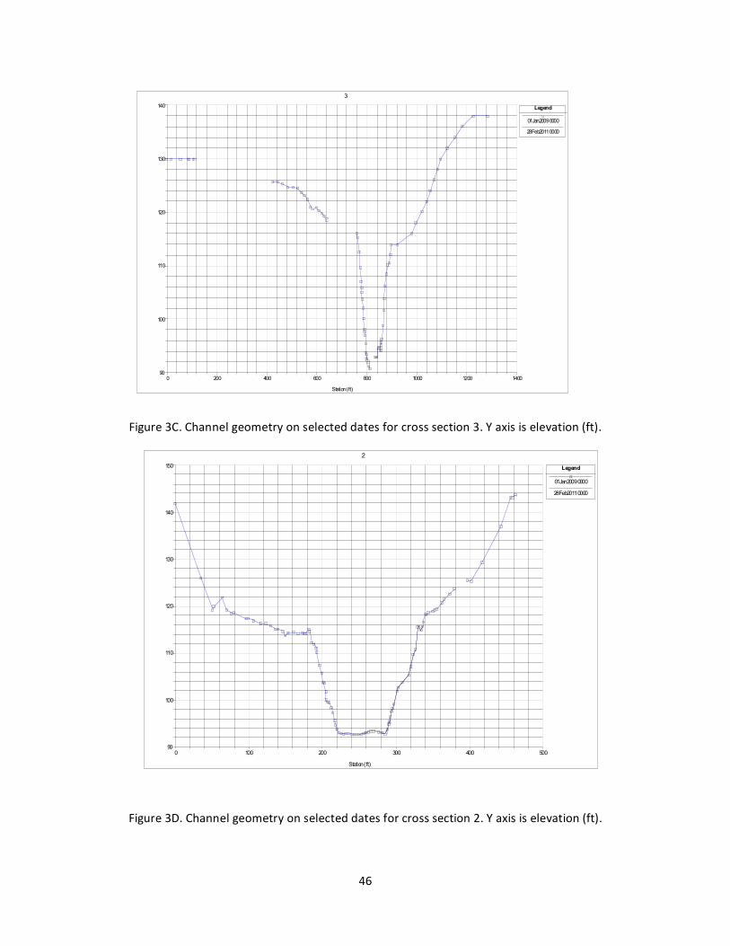
Figure 3C. Channel geometry on selected dates for cross section 3. Y axis is elevation (ft).

0 100 200 300 400 500 90

100

110

120

130

140

150

2

Station(ft)

Legend

01Jan20090000

28Feb20110000

Figure 3D. Channel geometry on selected dates for cross section 2. Y axis is elevation (ft).

46

 

Elevation

(ft)

0 100 200 300 400 500 80

90

100

110

120

130

140

150

1

Station(ft)

Legend

01Jan20090000

28Feb20110000

Figure 3E. Channel geometry on selected date for cross section 1. Y axis is elevation (ft).

47