SANDIA REPORT SAND2004-6635 Unlimited Release Printed December 2004

Final Report: Compliant Thermo-Mechanical MEMS Actuators LDRD #52553

Michael S. Baker, Richard A. Plass, Thomas J. Headley, Jeremy A. Walraven

Prepared by Sandia National Laboratories Albuquerque, New Mexico 87185 and Livermore, California 94550

Sandia is a multi-mission laboratory operated by Sandia Corporation, a Lockheed Martin Company, for the United States Department of Energy’s National Nuclear Security Administration under Contract DE-AC04-94AL85000.

Approved for public release; further dissemination unlimited.

Issued by Sandia National Laboratories, operated for the United States Department of Energy by

Sandia Corporation.

NOTICE: This report was prepared as an account of work sponsored by an agency of the United

States Government. Neither the United States Government, nor any agency thereof, nor any of

their employees, nor any of their contractors, subcontractors, or their employees, make any

warranty, express or implied, or assume any legal liability or responsibility for the accuracy,

completeness, or usefulness of any information, apparatus, product, or process disclosed, or

represent that its use would not infringe privately owned rights. Reference herein to any specific

commercial product, process, or service by trade name, trademark, manufacturer, or otherwise,

does not necessarily constitute or imply its endorsement, recommendation, or favoring by the

United States Government, any agency thereof, or any of their contractors or subcontractors. The

views and opinions expressed herein do not necessarily state or reflect those of the United States

Government, any agency thereof, or any of their contractors.

Printed in the United States of America. This report has been reproduced directly from the best

available copy.

Available to DOE and DOE contractors from

U.S. Department of Energy

Office of Scientific and Technical Information

P.O. Box 62

Oak Ridge, TN 37831

Telephone: (865)576-8401

Facsimile: (865)576-5728

E-Mail: reports@adonis.osti.gov

Online ordering: http://www.osti.gov/bridge

Available to the public from

U.S. Department of Commerce

National Technical Information Service

5285 Port Royal Rd

Springfield, VA 22161

Telephone: (800)553-6847

Facsimile: (703)605-6900

E-Mail: orders@ntis.fedworld.gov

Online order: http://www.ntis.gov/help/ordermethods.asp?loc=7-4-0#online

2

3

SAND2004-6635

Unlimited Release

Printed December 2004

Final Report: Compliant Thermo-Mechanical MEMS

Actuators LDRD #52553

Michael S. Baker

MEMS Device Technologies

Richard A. Plass

Radiation and Reliability Physics

Thomas J. Headley

Materials Characterization Department

Jeremy A. Walraven

Failure Analysis

Sandia National Laboratories

P.O. Box 5800

Albuquerque, NM 87185-1310

Abstract

Thermal actuators have proven to be a robust actuation method in surface-micromachined

MEMS processes. Their higher output force and lower input voltage make them an attractive

alternative to more traditional electrostatic actuation methods. A predictive model of thermal

actuator behavior has been developed and validated that can be used as a design tool to

customize the performance of an actuator to a specific application. This tool has also been used

to better understand thermal actuator reliability by comparing the maximum actuator temperature

to the measured lifetime.

Modeling thermal actuator behavior requires the use of two sequentially coupled models, the first

to predict the temperature increase of the actuator due to the applied current and the second to

model the mechanical response of the structure due to the increase in temperature. These two

models have been developed using Matlab for the thermal response and ANSYS for the

structural response. Both models have been shown to agree well with experimental data.

In a parallel effort, the reliability and failure mechanisms of thermal actuators have been studied.

Their response to electrical overstress and electrostatic discharge has been measured and a study

has been performed to determine actuator lifetime at various temperatures and operating

4

conditions. The results from this study have been used to determine a maximum reliable

operating temperature that, when used in conjunction with the predictive model, enables us to

design in reliability and customize the performance of an actuator at the design stage.

Acknowledgment

The authors would like to thank all of the staff in the MDL for fabrication and release/dry/coat

support through out this project. We would also like to thank Ken Pohl, Mark Jenkins and David

Luck for their assistance in testing and characterization, Mike Rye for TEM sample preparation,

and Hoshang (Amir) Shahvar and Ted Parson for their work in getting SHiMMeR operational

and configured for this experiment. Also, thanks to Sean Kearney and Leslie Phinney for their

work in collecting the Raman temperature data.

5

Contents

1. Introduction....................................................................................................................... 7

1.1. Thermal actuator designs .......................................................................................... 7

2. Model Development.......................................................................................................... 8

2.1. Material properties .................................................................................................... 9

2.1.1. Young’s Modulus.............................................................................................. 9

2.1.2. Resistivity ......................................................................................................... 9

2.1.3. Thermal conductivity ...................................................................................... 10

2.1.4. Coefficient of thermal expansion.................................................................... 10

2.2. Electro-thermal modeling ....................................................................................... 11

2.2.1. Thermal conduction shape-factor ................................................................... 13

2.3. Thermo-mechanical modeling ................................................................................ 13

2.4. Model Validation .................................................................................................... 14

2.4.1. Displacement and Resistance vs. Input Current ............................................. 14

2.4.2. Output Force vs. Input Current and Displacement ......................................... 16

2.4.3. Temperature Measurements............................................................................ 18

3. Reliability........................................................................................................................ 19

3.1. Short-term Discovery Experiments......................................................................... 19

3.1.1. Discussion of Short-term Experiments ........................................................... 22

3.2. Long-Term Reliability Test .................................................................................... 22

3.2.1. Long-Term Test Results – Deformation ......................................................... 27

3.2.2. Long-Term Test Results – Oxidation ............................................................. 29

3.2.3. Cycling Experiments....................................................................................... 33

3.3. Vacuum Experiments.............................................................................................. 34

3.4. Electrostatic Discharge Studies............................................................................... 34

4. Conclusions..................................................................................................................... 35

4.1. Future work............................................................................................................. 36

5. References....................................................................................................................... 36

6. Distribution List .............................................................................................................. 38

Figures

Figure 1-1: Illustration showing U shaped thermal actuator. ................................................... 7

Figure 1-2: Illustration of V shaped actuator. ........................................................................... 8

Figure 2-1: Representation of finite-difference element showing heat transfer terms. .......... 11

Figure 2-2: SEM image showing a typical thermal actuator design. ...................................... 14

Figure 2-3: Illustration showing dimension labels for SUMMiT actuator designs. .............. 15

Figure 2-4: Plots showing model predictions compared with measured data. Red line

indicates predicted temperature of 550° C...................................................................... 16

Figure 2-5: SEM showing force-gauge attached to actuator. ................................................. 17

Figure 2-6: Output force data compared to model predictions. .............................................. 17

Figure 2-7: IR image of a heated thermal actuator. ................................................................ 18

6

Figure 2-8: Plot of modeled temperatures vs. measured temperature using Raman

microscope. ..................................................................................................................... 19

Figure 3-1: a) SEM of actuator tested. b) Plot of shuttle displacement vs. applied power for

unloaded (open squares) and loaded (open triangles) actuators. Predicted displacement

for unloaded case is shown with solid squares. .............................................................. 20

Figure 3-2: Optical images of a) a pristine actuator, b) the same actuator at 302 mW applied

power (note the legs are glowing), c) the same actuator after power was turned off. d)-f)

the same power sequence for a loaded actuator of similar design (the load structure is

not shown). g) Plot of final rest positions after power cycle vs. power level. ................ 21

Figure 3-3: Thermal actuator test circuit diagram .................................................................. 24

Figure 3-4: Photograph of the SHiMMeR test system............................................................ 25

Figure 3-5: Rate of deformation as a function of maximum temperature .............................. 29

Figure 3-6: a) Optical image of actuator after continuous operation in air at 50% relative

humidity for six days at ~600° C maximum leg temperature. b) TEM showing oxide

growth at hottest part of an actuator leg and c) cross-section of same actuator taken near

the anchor where the polysilicon does not reach high temperatures. ............................. 30

Figure 3-7: Rate of oxidation as a function of maximum temperature................................... 31

Figure 3-8: a) optical image of an actuator after 31 million cycles. b) The same device after

an additional 42 million cycles. c) and d) SEM images showing wear debris and

substrate grooves............................................................................................................. 32

Figure 3-9: Overview of wear debris accumulation from an unloaded actuator after 1 billion

cycles when operated in dry nitrogen at ~550 C maximum leg temperature. ................ 33

Figure 3-10: a) Optical image of a loaded actuator before actuation. b) and c) show the same

actuator after 54 thousand actuation cycles under vacuum. d) Optical close-up image

after an additional 54 thousand cycles during which the device failed. e) SEM image of

cleaved actuator leg. f) SEM showing narrow transition between undamaged leg on

right and pitted surface on left. ....................................................................................... 34

Figure 3-11: SEM images showing brittle fracture after ESD testing. ................................... 35

Tables

Table 3-1: Test matrix for long-term experiments. Bold values indicate baseline geometries.

Approx. 720 actuators were included in this study......................................................... 23

Table 3-2: Plastic deformation rate activation energies – microns/day.................................. 28

Table 3-3: Oxidation activation energies - ∆R2/day ............................................................... 31

7

1. Introduction

MEMS motion and actuation has traditionally been achieved electrostatically using comb-

drive or parallel-plate actuation techniques. While successful, this actuation method

typically provides a small force per unit area and requires a high actuation voltage. Surface

micromachined electro-thermo-mechanical actuator designs can overcome these

disadvantages, providing a 100X higher output force, 10 X lower actuation voltages,

stictionless motion, and smaller consumed area on the die.

In this work we have developed a predictive modeling capability that will enable the design

of thermal actuators that overcome the disadvantage of high power consumption while

continuing to provide an order of magnitude higher force output and improved displacement

characteristics than their electrostatic counterparts. This model has been validated against

experimental data across a broad design space. In addition we have conducted a science-

based study of the reliability and predictability of thermally activated MEMS structures after

repeated thermal cycling. This study will be broadly applicable to any thermal MEMS

device.

1.1. Thermal actuator designs

Surface-micromachined thermal actuators utilize constrained thermal expansion to achieve

amplified motion. The thermal expansion is most commonly caused through Joule heating

by passing a current through thin actuator beams. There are two different thermal actuator

designs that have been demonstrated and commonly used in the literature, the pseudo-

bimorph or “U” shaped actuator [1-4], and the bent-beam or “V” shaped actuator [5-9]. Both

designs amplify the small input displacement created by thermal expansion, at the expense of

a reduction in the available output force.

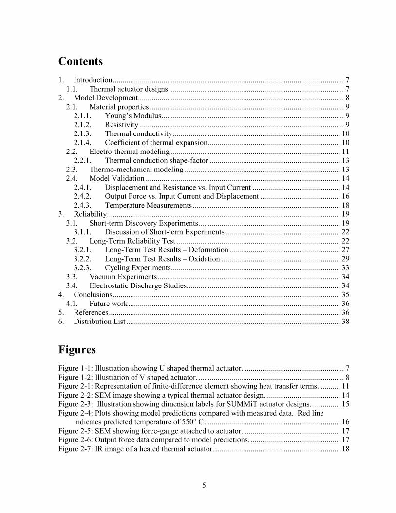
The U shaped actuator operation, illustrated in Figure 1-1, relies on creating a temperature

Figure 1-1: Illustration showing U shaped thermal actuator.

Anchored

contact pads

Hot-arm

Cold-arm

Motion

direction

8

difference between a hot-arm and cold-arm segment. The temperature difference is due to

the reduction in Joule heating in the cold-arm because of its decrease in electrical resistance

resulting from the increase in cross-sectional area. This results in a thermal expansion

difference between the two segments. Because both segments are constrained at their base

the actuator end experiences a rotary motion. Multiple actuators can be connected together

in parallel to increase the output force and to create a linear output motion if desired [3].

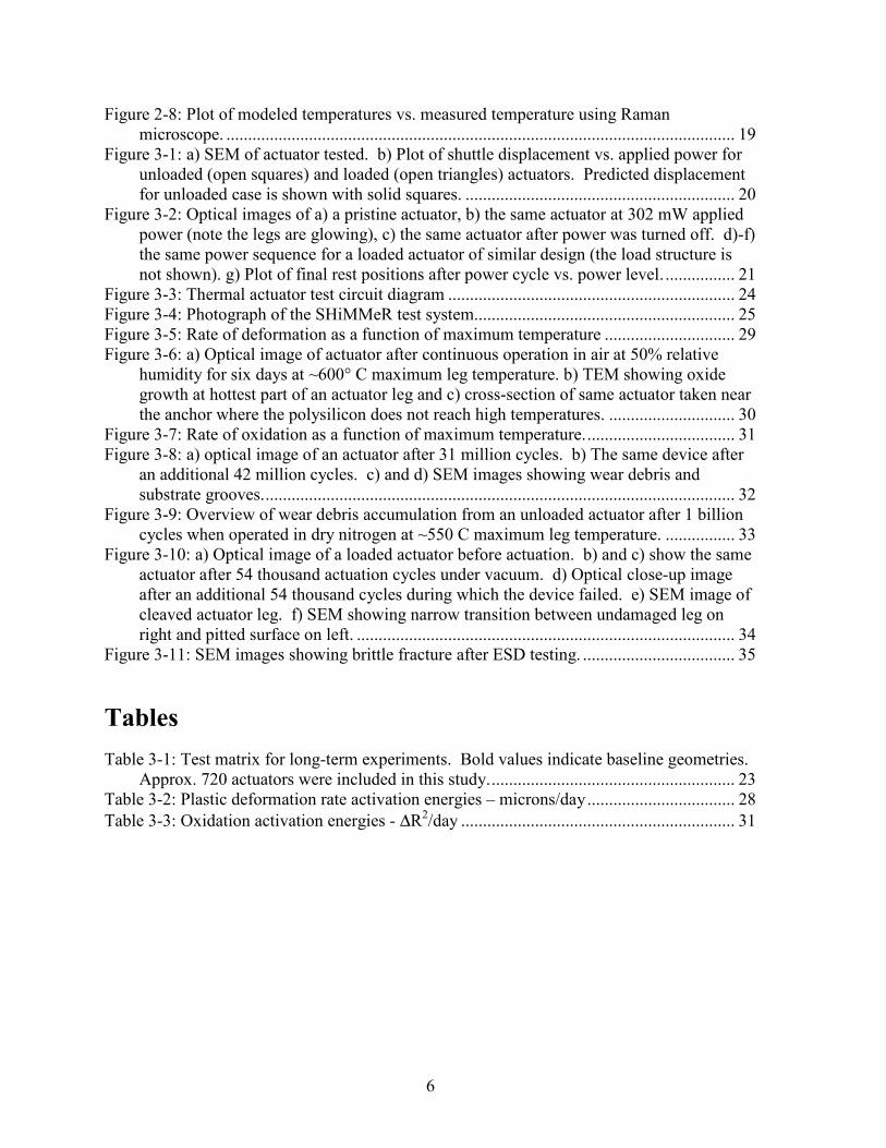
The V shaped, or chevron style actuator is illustrated in Figure 1-2. This design is

characterized by one or more V shaped beams, also commonly called legs, arranged in

parallel. As current is passed through the beams they heat and expand, and because of the

shallow angle of the beams, the center shuttle experiences an amplified displacement in the

direction of the offset.

This work will focus on the V style actuator as it has proven to be robust and offers design

flexibility. While micro-machined thermal actuators can be fabricated out of several

different materials depending on the MEMS process used, this work will focus on polysilicon

actuators fabricated in the Sandia National Laboratories SUMMiT VTM

process.

2. Model Development

There are many parameters that can be modified in the design of a V shaped thermal

actuator, including leg length and offset, leg cross-sectional area, and number of parallel legs.

A general knowledge of these parameters and their effect on actuator performance is

important to understand the trade-off’s required in the design process. In general, the

displacement of the center shuttle of a V style actuator increases with increased leg length

Figure 1-2: Illustration of V shaped actuator.

Applied voltage

Anchored

contact pad

Direction of

motion Movable

shuttle

Heated

beams

Heated

beams

9

and decreased leg offset angle. The displacement is insensitive to the cross-sectional area of

the legs and is not affected by the number of parallel legs. Because the actuator is essentially

a displacement amplifier (amplifying the small displacement due to thermal expansion into a

larger output displacement of the center shuttle), it is expected that any change which

increases the output displacement will decrease the output force. This is indeed the case as

the output force of the actuator will decrease with increased leg length and decreased leg

offset. However, while the displacement is insensitive to the cross-sectional area of the legs

and to the number of parallel legs, the output force is very sensitive to these parameters. The

output force is limited essentially by the buckling strength of the legs and so increasing the

cross-sectional area will stiffen the actuator and increase the available output force. Also, the

force increases linearly with the number of parallel legs.

While the general design trends described above can act as a guide in actuator design,

thermal actuators are inherently non-linear and an accurate prediction of their behavior

requires a detailed model. To capture all of the relevant effects, a thermal actuator model

must couple several different physics, including the electrical, thermal and mechanical

domains. Because of this, it is difficult to derive a closed-form solution that can adequately

model device performance; however, numerical models have been used with success. These

range from finite-difference approaches to full three-dimensional finite element solutions

[10-12].

This work will describe the development of a custom finite-difference electro-thermal model

that is coupled to a commercial finite-element solution for the thermo-mechanical problem.

The results of this model show good agreement with experimental data. A discussion of the

relevant material properties for this analysis will be followed by a detailed description of the

modeling technique and validation.

2.1. Material properties

Regardless of the model complexity, an analysis can only be as accurate as the model inputs.

For this reason it is important that accurate material properties be know for the materials used

in a thermal actuator. In this work all actuators are fabricated in the Sandia National

Laboratories SUMMiT VTM

sacrificial surface micromachined process [13]. In this process

the structural material is polysilicon, and relevant properties are given for this material set.

2.1.1. Young’s Modulus

Young’s Modulus is an important property in the structural modeling step. It is a measure of

the inherent stiffness of a material and affects both the displacement and output force

predicted by the model. Its magnitude will be a function of the fabrication process, and it has

been measured on SUMMiT VTM

parts to be 164.3 GPa ± 3.2 GPa [14].

2.1.2. Resistivity

The heat used to drive a thermal actuator is generated by resistive heating. For this reason,

the material resistivity is an important property in correctly modeling the temperature rise of

the actuator due to the applied voltage. Because thermal actuators can reach temperatures in

excess of 600 C, this property should be known as a function of temperature. For

polysilicon, the resistivity is determined by process parameters and dopant levels, with

10

SUMMiT VTM

polysilicon being highly n-type doped. Its resistivity was measured using

standard van der Pauw sheet-resistance structures [15,16] from room temperature up to

550° C for all three of the primary structural layers (Poly1/2 laminate, poly3 and poly4). A

curve fit of this data, averaged across all three layers is defined as

If T<300 Eq. 2-1

858.20)109713.2( 2 +×= − Tρ

If T>300 and T<700

402.26)102473.7()101600.6( 325 +×−×= −− TTρ

If T>700

8551.8)10624.8( 2 −×= − Tρ

where the temperature is in degrees Celsius and the resistivity is in units of ohm-microns.

The curve fit extends above 700° C to help with model convergence during non-linear

iterations but should not be considered accurate above 600 C. It is interesting to note that

resistance increases with increasing temperature linearly up to approximately 300° C, where

the dependence becomes quadratic. At room temperature the resistivity is 21.5 ohm-microns.

2.1.3. Thermal conductivity

Again, because of the high temperatures possible during thermal actuator operation, the

thermal conductivity of the structural material and the surrounding medium (typically air or

vacuum) should be known as a function of temperature. Measurements have been made on

Sandia large-grained polysilicon [17] up to 700 K, with the curve fit reported for this data as

014.0)100.1()100.9()102.2(

1528311 +×−×+×−

=−−− TTT

k p Eq. 2-2

where the temperature is in degrees Celsius and the thermal conductivity is in W/m/°C. At

room temperature the thermal conductivity of polysilicon is 72 W/m/°C, and it decreases

with increasing temperature.

Data on the thermal conductivity of air is readily available [18], and is given as

3428311 102076.5)102940.1()101803.9()104288.3( −−−− ×−×+×−×= TTTka Eq. 2-3

where the temperature is in degrees Kelvin and the conductivity is in W/m/°C. At room

temperature the thermal conductivity of air is 0.026 W/m/°C and it increases with increased

temperature.

2.1.4. Coefficient of thermal expansion

The instantaneous coefficient of thermal expansion has been measured on single crystal

silicon up to 1500 K, and the corresponding curve fit is given as

11

( )( )( )( ) 643 10)10548.5(1251088.5exp1725.3 −−− ××+−×−−×= TTIα Eq. 2-4

where the temperature is given in Kelvin [19]. To calculate the total elongation of a sample

due to a temperature change, the instantaneous CTE must be integrated across the

temperature range using the following equation,

∫=−T

TI dTTLLL

000 )(α Eq. 2-5

Where L0 is the zero-stress length at temperature T0, and L is the new length at temperature T.

At room temperature the CTE of polysilicon is 2.5×10-6 C

-1 and it increases with

temperature.

2.2. Electro-thermal modeling

The electro-thermal portion of the modeling problem has been solved using a custom finite-

difference formulation that is specific to the geometry of the V shaped actuator. With this

approach, the actuator legs are equally divided into a number of serially connected finite-

difference elements with a temperature node located at the center of each element. The

temperature of the finite-difference node represents the average temperature of the element

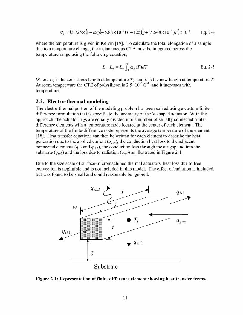
[18]. Heat transfer equations can then be written for each element to describe the heat

generation due to the applied current (qgen), the conduction heat loss to the adjacent

connected elements (qi-1 and qi+1), the conduction loss through the air gap and into the

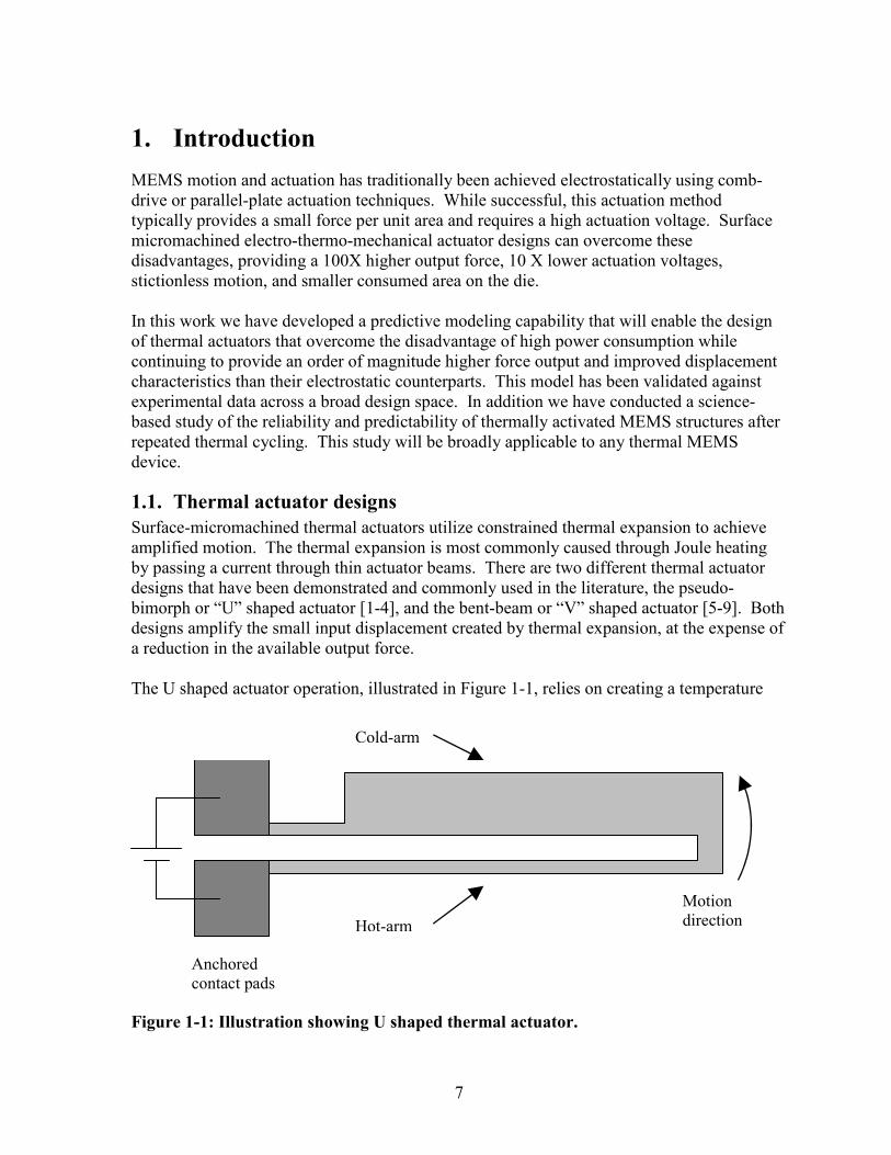
substrate (qsub) and the loss due to radiation (qrad) as illustrated in Figure 2-1.

Due to the size scale of surface-micromachined thermal actuators, heat loss due to free

convection is negligible and is not included in this model. The effect of radiation is included,

but was found to be small and could reasonable be ignored.

Figure 2-1: Representation of finite-difference element showing heat transfer terms.

g

Ti

qi+1

qi-1

qsub

qgen

x qrad

w

t

Substrate

12

An equation for each of the heat transfer terms shown in Figure 2-1 can be written as follows

x

TTAkq

iixp

i

)( 1

1

+

+

−= Eq. 2-6

x

TTAkq

iixp

i

)( 1

1

−

−

−= Eq. 2-7

g

TTASkq subibasub

)( −= Eq. 2-8

)( 44

subisrad TTAq −= σε Eq. 2-9

x

genA

xiq

2ρ= Eq. 2-10

where x is the distance between finite-difference nodes, kp is the thermal conductivity of

polysilicon, ka is the thermal conductivity of the surrounding air, Ax is the cross-sectional

area of the actuator beam, Ab is the surface area of the bottom of the finite-difference element

(wx for the rectangular cross-section shown in Figure 2-1), As is the total surface area of the

finite-difference element, S is the conduction shape factor for the cross-section as explained

in Section 2.2.1, σ is the Stefan-Boltzmann constant of 5.670×10-8 W/m

2/K

4, ε is the

emissivity of polysilicon, i is the applied current, and ρ is the resistivity of polysilicon.

In steady-state thermal equilibrium, the sum of the heat loss terms must equal the heat

generated,

genradsubii qqqqq =+++ −+ 11 Eq. 2-11

This equilibrium equation can be written for each finite-difference node, where the only

unknown is the temperature at each node. If the heated actuator leg is divided into n finite-

difference elements, there will be n equations with n unknown temperatures. This linear

system of equations can be solved using traditional linear algebra techniques [20] to

determine the temperature at each node. To account for the temperature dependent material

properties, iteration is required. The resistivity and thermal conductivity is re-evaluated at

each node after each iteration until the solution converges.

Because the actuator is symmetric about the center shuttle, modeling one half of the actuator

is sufficient. In designs that use multiple parallel actuator beams, each beam behaves the

same. The complete solution is thus obtained by modeling only a single heated beam from

the anchor to the centerline of the actuator. This reduction minimizes the number of

simultaneous equations that must be solved, reducing computational expense. For more

accurate results, thermal conduction through the anchor pad and center shuttle can be

modeled as well using the same finite-difference technique.

13

2.2.1. Thermal conduction shape-factor

The technique for modeling the heat transfer in a thermal actuator beam is a 1-dimensional

solution along the beam length. It assumes that the temperature is uniform across the beam

cross-section and is appropriate as the cross-sectional dimension is typically much smaller

than the length. However, when operating in air, one of the dominant heat loss mechanisms

is conduction through the air to the substrate. The rate of heat loss by this mechanism

depends on the cross-sectional shape of the beam and the gap to the substrate, which requires

a 2-dimensional solution. To address this issue while maintaining the speed and flexibility of

the 1-D finite-difference solution, a 2-D conduction shape factor is used to account for the

additional conductive heat losses from the sides and top of the beam. This shape factor is

defined as the ratio of the total heat loss divided by the heat loss from only the bottom

surface [18,21]. It is specific to a given cross-sectional shape. For some shapes this factor

can be determined using a closed form solution, but typically it is found using finite-element

analysis techniques for the cross-section of interest.

To allow the solution to remain fully parametric, the shape factor was determined by finite-

element analysis for a range of rectangular cross-sections. A total of 570 finite-element

solutions were performed for the range of 0.65 < t/w < 6.4 and 0.15 < g/t < 5.9. These results

were then curve-fit to allow the shape factor to be quickly determined for any actuator cross-

section within the SUMMiT VTM

design space. The curve fit for the shape factor is given as

+

+

+

−

×+

×−= −−

w

t

t

g

t

g

t

g

t

gS 31096.06828.253515.0101051.9109062.5

23

2

4

3

+

+

×− − 99313.040393.0104102.2

2

2

t

g

t

g Eq. 2-12

where g is the gap, t is the thickness, and w is the width as shown in Figure 2-1.

2.3. Thermo-mechanical modeling

From the electro-thermal modeling, the temperature profile of the heated actuator legs is

obtained, and becomes the input for the thermo-mechanical solution. The first step in this

model is to determine the total thermal strain in the actuator by summing the change in

length, L-L0, for each of the finite-difference elements in the electro-thermal solution using

Eq. 2-5. The value must be calculated for each individual element and summed due to the

temperature dependent nature of the coefficient of thermal expansion. Any residual stress

inherent in the polysilicon due to the fabrication process can be added to the thermally

induced stress at this point to improve the accuracy of the final solution.

The structural response of the actuator can be determined using traditional finite-element

analysis (FEA). Because of the long, slender nature of thermal actuators, it is appropriate to

use beam elements in the FEA solution to reduce computational expense, and is consistent

with the use of beams in the electro-thermal solution. With the simple geometry, an input

file can be created for most commercial FEA codes to allow for the entire solution to be

parametrically driven for rapid design evaluations. This is important for design optimization

and uncertainty analyses. For this work the commercial code ANSYS was used for the

14

structural response. Material stresses, displacements and output forces can all be obtained

from the FEA solution.

The output force of a thermal actuator is a non-linear function of both the applied electrical

power and the displacement. Therefore, the finite-element solver must be capable of

performing non-linear iterations. The output force curve is then determined by allowing the

actuator to fully expand to its unloaded maximum displacement and then pushing it back to

the zero-displacement position in the finite-element solution. The reaction load required to

push back on the actuator is extracted as the maximum output force at that displacement and

input power.

2.4. Model Validation

To verify that the model captures all the relevant physical effects, several different actuators

fabricated in the SUMMiT VTM

process were compared to model predictions, including the

displacement, total actuator resistance and leg temperature as a function of the input current

and output fo rce as a function of both position and input current. A total of twenty different

actuator designs, with different actuator lengths, offsets, gaps (done by changing the

SUMMiT layer used for the device), and cross-sectional areas, were fabricated at tested.

Results are reported for a single representative design in each section. The cross-section

thicknesses and gap are defined by the SUMMiT layers used. The I-beam shape produced

using the P1P2 laminate layer and the P3 layer together increases the out-of-plane stiffness of

the actuator.

2.4.1. Displacement and Resistance vs. Input Current

The most direct validation of the model is obtained by comparing the measured output

displacement with applied current to model predictions. The displacement is directly

measurable experimentally and represents the final cumulative output of each part of the

model. For this work, the displacement was measured using a National Instruments Vision

software package that performs sub-pixel image tracking. A 200X magnification was used to

minimize the displacement measurement error to less than ±0.25 microns. Results are shown

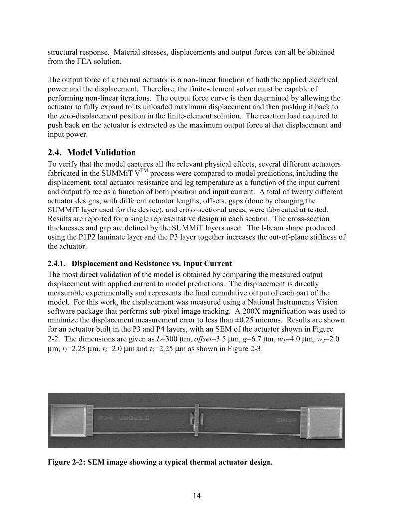
for an actuator built in the P3 and P4 layers, with an SEM of the actuator shown in Figure

2-2. The dimensions are given as L=300 µm, offset=3.5 µm, g=6.7 µm, w1=4.0 µm, w2=2.0

µm, t1=2.25 µm, t2=2.0 µm and t3=2.25 µm as shown in Figure 2-3.

Figure 2-2: SEM image showing a typical thermal actuator design.

15

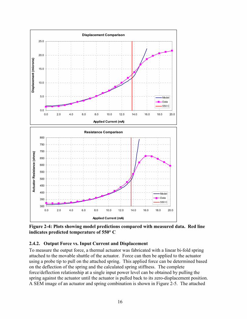
Displacement and resistance measurements were collected at three locations on the wafer and

the measurements were repeatable to better than the measurement accuracy. In each of the

three measurements, the actuators had not been previously powered to ensure undamaged

devices for testing. The current was stepped up in increments of one milliamp until the

device failed, with the displacement and resistance measured at each current level. Plots of

the measured and modeled response for both displacement and resistance are shown in

Figure 2-4. It is important to note that the modeled curves were generated using the nominal

process parameters for thickness and width. These parameters are known to vary due to the

chemical-mechanical polishing process step that defines the oxide thickness, and the edge

bias in the etch that defines the widths.

The vertical red line in the plot indicates the current level resulting in a predicted temperature

of 550° C. This is the maximum temperature with available resistivity data. Above this

point the roll-off in displacement and resistance in the measured data is attributed to high

temperatures that result in melting of the polysilicon. This is visually confirmed as the

actuators begin to glow red at this point, indicating operation near the melting point. In all

data sets, the model tends to under-predict the displacement and resistance at temperatures

nearing the 550° C threshold. At these high temperatures the model becomes very sensitive

to the cross-sectional area of the actuator leg, and therefore sensitive to variations in the

process that defines this cross-section. The differences observed between the model and data

in Figure 2-4 can be eliminated by adjusting the actuator width and layer thicknesses in the

model within the known process variation. For the model to serve as a robust design tool, an

uncertainty analysis should be performed to determine the expected error bounds for the

predicted performance due to process variations.

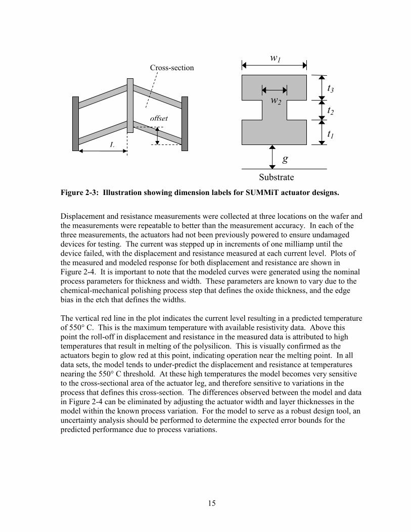
Figure 2-3: Illustration showing dimension labels for SUMMiT actuator designs.

w1

g

t1

t2

t3 w2

Substrate

Cross-section

offset

L

16

2.4.2. Output Force vs. Input Current and Displacement

To measure the output force, a thermal actuator was fabricated with a linear bi-fold spring

attached to the movable shuttle of the actuator. Force can then be applied to the actuator

using a probe tip to pull on the attached spring. This applied force can be determined based

on the deflection of the spring and the calculated spring stiffness. The complete

force/deflection relationship at a single input power level can be obtained by pulling the

spring against the actuator until the actuator is pulled back to its zero-displacement position.

A SEM image of an actuator and spring combination is shown in Figure 2-5. The attached

Figure 2-4: Plots showing model predictions compared with measured data. Red line

indicates predicted temperature of 550° C

Displacement Comparison

0.0

5.0

10.0

15.0

20.0

25.0

0.0 2.0 4.0 6.0 8.0 10.0 12.0 14.0 16.0 18.0 20.0

Applied Current (mA)

Displacement (m

icrons)

Model

Data

550 C

Resistance Comparison

300

350

400

450

500

550

600

650

700

750

800

0.0 2.0 4.0 6.0 8.0 10.0 12.0 14.0 16.0 18.0 20.0

Applied Current (mA)

Actuator Resistance (ohms)

Model

Data

550 C

17

force-gauge spring was designed using an uncertainty analysis technique to minimize the

uncertainty in the spring constant due to variations in the process [22].

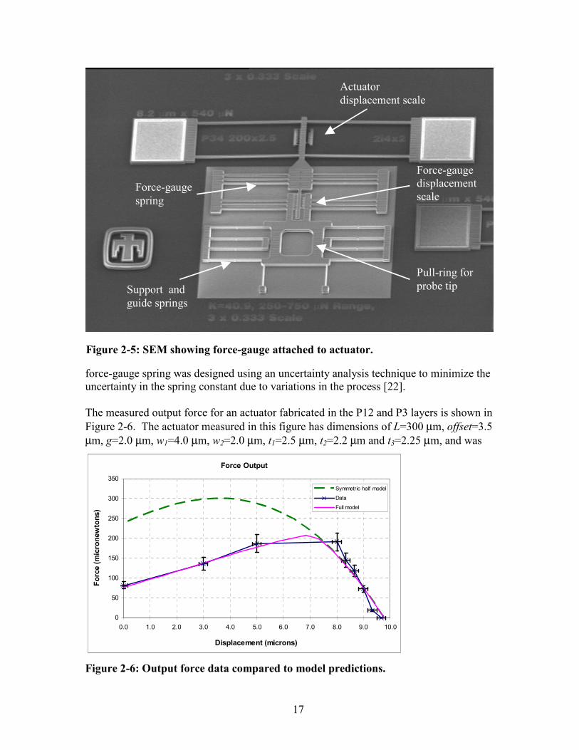
The measured output force for an actuator fabricated in the P12 and P3 layers is shown in

Figure 2-6. The actuator measured in this figure has dimensions of L=300 µm, offset=3.5

µm, g=2.0 µm, w1=4.0 µm, w2=2.0 µm, t1=2.5 µm, t2=2.2 µm and t3=2.25 µm, and was

Figure 2-5: SEM showing force-gauge attached to actuator.

Figure 2-6: Output force data compared to model predictions.

Force-gauge

spring

Actuator

displacement scale

Force-gauge

displacement

scale

Pull-ring for

probe tip Support and

guide springs

Force Output

0

50

100

150

200

250

300

350

0.0 1.0 2.0 3.0 4.0 5.0 6.0 7.0 8.0 9.0 10.0

Displacement (microns)

Force (micronewtons)

Symmetric half model

Data

Full model

18

actuated at a constant 15 mA at 6.1 V. There are two predicted curves for the force output,

illustrating an important consideration when modeling the output force of a thermal actuator.

The green dashed curve labeled “symmetric half-model” is the predicted force output when

modeling only a single beam with a symmetry plane down the center of the actuator so as to

model only half of the actuator length. Utilizing symmetry in this manner is a common

analysis technique as it reduces the problem size. But when pushing against a load, a thermal

actuator will often buckle in a non-symmetric fashion resulting in a force output lower than

predicted by a purely symmetric model. This could be due to slight variations in the leg

widths or thicknesses or from a non-ideal application of the load against the actuator. The

purple curve labeled “full model” was modeled using a full-actuator model (no symmetry

planes), with the force applied at a slight offset from center to introduce an asymmetry. This

results in a predicted force output curve that is significantly lower than the ideal symmetric

case, but that matches very well with experimental data.

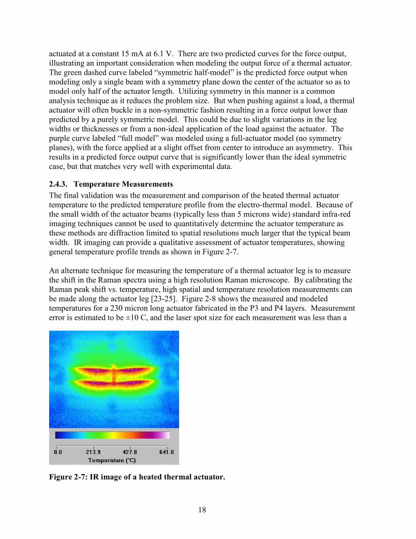
2.4.3. Temperature Measurements

The final validation was the measurement and comparison of the heated thermal actuator

temperature to the predicted temperature profile from the electro-thermal model. Because of

the small width of the actuator beams (typically less than 5 microns wide) standard infra-red

imaging techniques cannot be used to quantitatively determine the actuator temperature as

these methods are diffraction limited to spatial resolutions much larger that the typical beam

width. IR imaging can provide a qualitative assessment of actuator temperatures, showing

general temperature profile trends as shown in Figure 2-7.

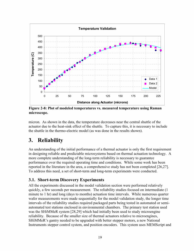
An alternate technique for measuring the temperature of a thermal actuator leg is to measure

the shift in the Raman spectra using a high resolution Raman microscope. By calibrating the

Raman peak shift vs. temperature, high spatial and temperature resolution measurements can

be made along the actuator leg [23-25]. Figure 2-8 shows the measured and modeled

temperatures for a 230 micron long actuator fabricated in the P3 and P4 layers. Measurement

error is estimated to be ±10 C, and the laser spot size for each measurement was less than a

Figure 2-7: IR image of a heated thermal actuator.

19

micron. As shown in the data, the temperature decreases near the central shuttle of the

actuator due to the heat-sink effect of the shuttle. To capture this, it is necessary to include

the shuttle in the thermo-electric model (as was done in the results shown).

3. Reliability

An understanding of the initial performance of a thermal actuator is only the first requirement

in designing reliable and predictable microsystems based on thermal actuation technology. A

more complete understanding of the long-term reliability is necessary to guarantee

performance over the required operating time and conditions. While some work has been

reported in the literature in the area, a comprehensive study has not been completed [26,27].

To address this need, a set of short-term and long-term experiments were conducted.

3.1. Short-term Discovery Experiments

All the experiments discussed in the model validation section were performed relatively

quickly, a few seconds per measurement. The reliability studies focused on intermediate (1

minute to 1 hr) and long (days to months) actuation time intervals. While numerous quarter

wafer measurements were made sequentially for the model validation study, the longer time

intervals of the reliability studies required packaged parts being tested in automated or semi-

automated test stations enclosed in environmental chambers. The primary test station used

was the SHiMMeR system [28,29] which had initially been used to study microengine

reliability. Because of the smaller size of thermal actuators relative to microengines,

SHiMMeR’s gantry needed to be upgraded with better stepper motors, a new National

Instruments stepper control system, and position encoders. This system uses MEMScript and

Figure 2-8: Plot of modeled temperatures vs. measured temperature using Raman

microscope.

Temperature Validation

0

50

100

150

200

250

300

350

400

450

500

0 25 50 75 100 125 150 175 200 225

Distance along Actuator (microns)

Temperature (C)

Data 1

Data 2

Model

20

NI Vision pattern matching routines to determine the displacement of the thermal actuator

shuttle relative to a fixed reference point in the field of view. Since thermal actuators require

current sources rather than the ~ 100 Volt waveforms previously required by microengines,

different device actuation electronics had to be installed. Because we also want to measure

the effective resistance change of the thermal actuators, a Racal multiplexer and a National

Instruments Data Acquisition card was added to the system. A fully automated test control

and optical data collection program was written in Labview.

In the first set of tests or “discovery” experiments, devices were subjected to sequentially

increasing actuation power levels (DC and square wave modulated at 30 or 500 Hz), in ~30%

relative humidity lab air, ~95% high humidity conditions, and vacuum conditions. The short-

term DC experiments were conducted as follows: the initial position of a packaged thermal

actuator was photographed and its two point resistance was measured. Then a specified

current was passed through the device for a set period of time, usually one minute, after

which time the device was again photographed and its voltage drop was measured. The

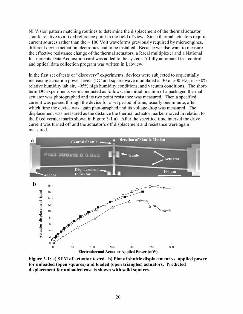
displacement was measured as the distance the thermal actuator marker moved in relation to

the fixed vernier marks shown in Figure 3-1 a). After the specified time interval the drive

current was turned off and the actuator’s off displacement and resistance were again

measured.

Figure 3-1: a) SEM of actuator tested. b) Plot of

for unloaded (open squares) and loaded (open tr

displacement for unloaded case is shown with so

0

2

4

6

8

10

12

14

16

18

0 50 100 150

Actuator displacemen

t (µm)

Anchor Indicator

a

b

Direction of Shuttle Motion

Electrothermal Actuator Ap

Guide

Legs Structu

100 µm

Displacement

shuttle displacem

iangles) actuators

lid squares.

200 250

plied Power (mW)

Actuator

Central Shuttle

ent vs. applied power

. Predicted

300

21

Shuttle displacements were obtained using National Instruments Vision image analysis

software routines [30]. The routines can resolve approximately one fifth of a pixel

displacement which, at the 400X magnification used, corresponds to about 0.1 µm. Shuttle

displacements were measured by comparing the images of stressed devices to unstressed

pristine devices. Relative position changes of the fixed vernier structures were used to

compensate for microscope stage drift. Figure 3-1 b) shows typical shuttle displacement

versus applied DC power curves for an unloaded (open squares) and a loaded (open triangles)

actuator with dimensions of L=300 µm, offset=12 µm, g=2.0 µm, w1=3.0 µm, w2=2.0 µm,

t1=2.5 µm, t2=2.2 µm and t3=2.25 µm (as shown in Figure 2-3). As expected, the

displacement versus power is almost linear up to about 200 mW, or approximately 705° C

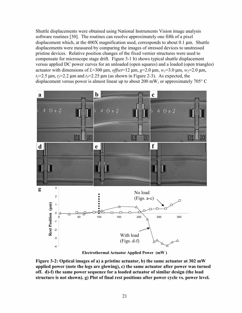
Figure 3-2: Optical images of a) a pristine actuator, b) the same actuator at 302 mW

applied power (note the legs are glowing), c) the same actuator after power was turned

off. d)-f) the same power sequence for a loaded actuator of similar design (the load

structure is not shown). g) Plot of final rest positions after power cycle vs. power level.

-4

-3

-2

-1

0

1

2

3

0 50 100 150 200 250 300

g

Electrothermal Actuator Applied Power (mW )

Rest Position (µm)

a b c

d e f

No load

(Figs. a-c)

With load

(Figs. d-f)

22

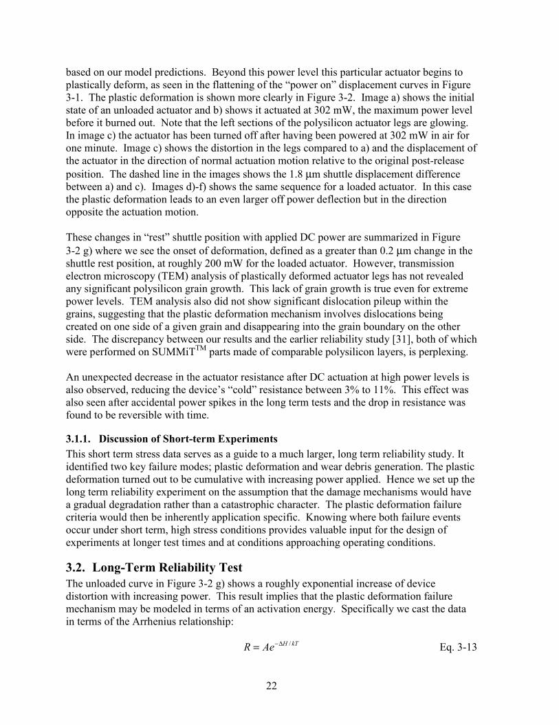
based on our model predictions. Beyond this power level this particular actuator begins to

plastically deform, as seen in the flattening of the “power on” displacement curves in Figure

3-1. The plastic deformation is shown more clearly in Figure 3-2. Image a) shows the initial

state of an unloaded actuator and b) shows it actuated at 302 mW, the maximum power level

before it burned out. Note that the left sections of the polysilicon actuator legs are glowing.

In image c) the actuator has been turned off after having been powered at 302 mW in air for

one minute. Image c) shows the distortion in the legs compared to a) and the displacement of

the actuator in the direction of normal actuation motion relative to the original post-release

position. The dashed line in the images shows the 1.8 µm shuttle displacement difference

between a) and c). Images d)-f) shows the same sequence for a loaded actuator. In this case

the plastic deformation leads to an even larger off power deflection but in the direction

opposite the actuation motion.

These changes in “rest” shuttle position with applied DC power are summarized in Figure

3-2 g) where we see the onset of deformation, defined as a greater than 0.2 µm change in the

shuttle rest position, at roughly 200 mW for the loaded actuator. However, transmission

electron microscopy (TEM) analysis of plastically deformed actuator legs has not revealed

any significant polysilicon grain growth. This lack of grain growth is true even for extreme

power levels. TEM analysis also did not show significant dislocation pileup within the

grains, suggesting that the plastic deformation mechanism involves dislocations being

created on one side of a given grain and disappearing into the grain boundary on the other

side. The discrepancy between our results and the earlier reliability study [31], both of which

were performed on SUMMiTTM

parts made of comparable polysilicon layers, is perplexing.

An unexpected decrease in the actuator resistance after DC actuation at high power levels is

also observed, reducing the device’s “cold” resistance between 3% to 11%. This effect was

also seen after accidental power spikes in the long term tests and the drop in resistance was

found to be reversible with time.

3.1.1. Discussion of Short-term Experiments

This short term stress data serves as a guide to a much larger, long term reliability study. It

identified two key failure modes; plastic deformation and wear debris generation. The plastic

deformation turned out to be cumulative with increasing power applied. Hence we set up the

long term reliability experiment on the assumption that the damage mechanisms would have

a gradual degradation rather than a catastrophic character. The plastic deformation failure

criteria would then be inherently application specific. Knowing where both failure events

occur under short term, high stress conditions provides valuable input for the design of

experiments at longer test times and at conditions approaching operating conditions.

3.2. Long-Term Reliability Test

The unloaded curve in Figure 3-2 g) shows a roughly exponential increase of device

distortion with increasing power. This result implies that the plastic deformation failure

mechanism may be modeled in terms of an activation energy. Specifically we cast the data

in terms of the Arrhenius relationship:

kTHAeR /∆−= Eq. 3-13

23

where R is the device degradation rate with time, A is a constant we will call the prefactor, k

is Boltzmann’s constant (8.617x10-5 eV / K), T is the temperature in degrees Kelvin, and ∆H

is the “activation energy”. This reliability based activation energy term should not be

confused with chemical reaction activation energies, though the damage mechanism may be

related to a chemical reaction, here the term activation energy is simply a way to reduce a

temperature based damage mechanism to a compact, useful mathematical description.

To determine A and ∆H as accurately as possible we need to find the thermal actuator

deformation rate over as broad a maximum leg temperature / power level range as possible.

Given the logarithmic nature of this function, we can foresee that collecting low temperature

deformation rates will require months of low power device actuation with relatively

infrequent data collection intervals while high temperature deformation rates can be collected

in hours or days but require short data collection intervals. Hence the lower power tests were

conducted by keeping powered devices in dry-box environmental chambers and periodically

inspecting them on a semi-automated probe station (SHiMMeR Lite), while the higher power

tests were conducted more rapidly in the fully automated SHiMMeR system.

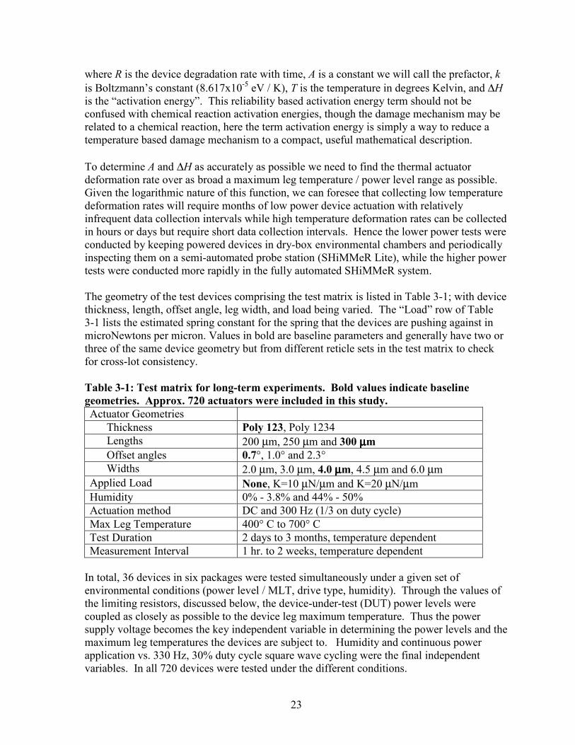
The geometry of the test devices comprising the test matrix is listed in Table 3-1; with device

thickness, length, offset angle, leg width, and load being varied. The “Load” row of Table

3-1 lists the estimated spring constant for the spring that the devices are pushing against in

microNewtons per micron. Values in bold are baseline parameters and generally have two or

three of the same device geometry but from different reticle sets in the test matrix to check

for cross-lot consistency.

Table 3-1: Test matrix for long-term experiments. Bold values indicate baseline

geometries. Approx. 720 actuators were included in this study.

Actuator Geometries

Thickness Poly 123, Poly 1234

Lengths 200 µm, 250 µm and 300 µµµµm

Offset angles 0.7°, 1.0° and 2.3°

Widths 2.0 µm, 3.0 µm, 4.0 µµµµm, 4.5 µm and 6.0 µm

Applied Load None, K=10 µN/µm and K=20 µN/µm

Humidity 0% - 3.8% and 44% - 50%

Actuation method DC and 300 Hz (1/3 on duty cycle)

Max Leg Temperature 400° C to 700° C

Test Duration 2 days to 3 months, temperature dependent

Measurement Interval 1 hr. to 2 weeks, temperature dependent

In total, 36 devices in six packages were tested simultaneously under a given set of

environmental conditions (power level / MLT, drive type, humidity). Through the values of

the limiting resistors, discussed below, the device-under-test (DUT) power levels were

coupled as closely as possible to the device leg maximum temperature. Thus the power

supply voltage becomes the key independent variable in determining the power levels and the

maximum leg temperatures the devices are subject to. Humidity and continuous power

application vs. 330 Hz, 30% duty cycle square wave cycling were the final independent

variables. In all 720 devices were tested under the different conditions.

24

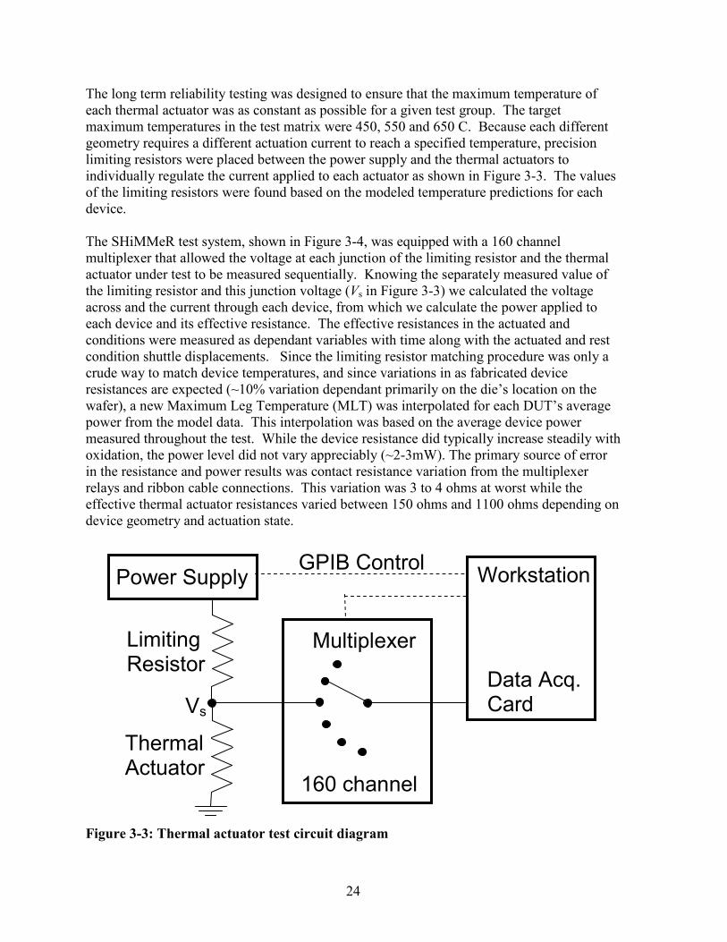
The long term reliability testing was designed to ensure that the maximum temperature of

each thermal actuator was as constant as possible for a given test group. The target

maximum temperatures in the test matrix were 450, 550 and 650 C. Because each different

geometry requires a different actuation current to reach a specified temperature, precision

limiting resistors were placed between the power supply and the thermal actuators to

individually regulate the current applied to each actuator as shown in Figure 3-3. The values

of the limiting resistors were found based on the modeled temperature predictions for each

device.

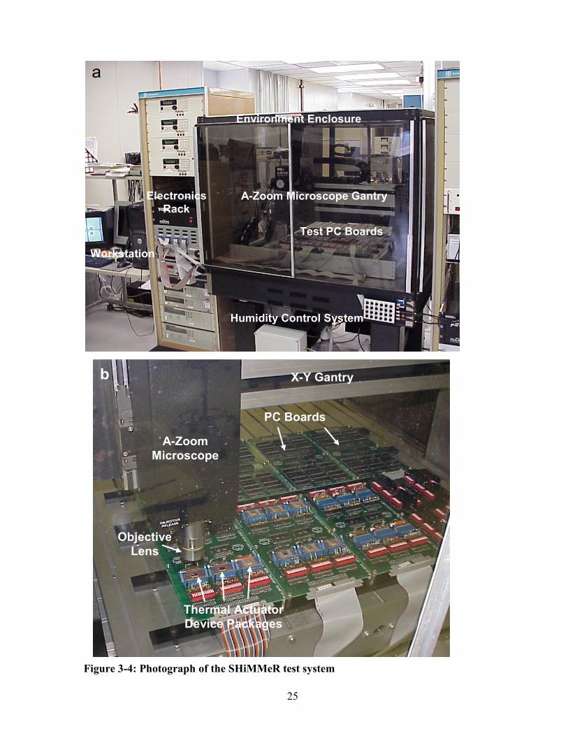
The SHiMMeR test system, shown in Figure 3-4, was equipped with a 160 channel

multiplexer that allowed the voltage at each junction of the limiting resistor and the thermal

actuator under test to be measured sequentially. Knowing the separately measured value of

the limiting resistor and this junction voltage (Vs in Figure 3-3) we calculated the voltage

across and the current through each device, from which we calculate the power applied to

each device and its effective resistance. The effective resistances in the actuated and

conditions were measured as dependant variables with time along with the actuated and rest

condition shuttle displacements. Since the limiting resistor matching procedure was only a

crude way to match device temperatures, and since variations in as fabricated device

resistances are expected (~10% variation dependant primarily on the die’s location on the

wafer), a new Maximum Leg Temperature (MLT) was interpolated for each DUT’s average

power from the model data. This interpolation was based on the average device power

measured throughout the test. While the device resistance did typically increase steadily with

oxidation, the power level did not vary appreciably (~2-3mW). The primary source of error

in the resistance and power results was contact resistance variation from the multiplexer

relays and ribbon cable connections. This variation was 3 to 4 ohms at worst while the

effective thermal actuator resistances varied between 150 ohms and 1100 ohms depending on

device geometry and actuation state.

Figure 3-3: Thermal actuator test circuit diagram

Thermal Actuator

Limiting Resistor

Vs

Power Supply

Multiplexer

Data Acq. Card

Workstation GPIB Control

160 channel

25

Figure 3-4: Photograph of the SHiMMeR test system

a

Workstation

Environment Enclosure

A-Zoom Microscope Gantry

Test PC Boards

Electronics

Rack

Humidity Control System

b

A-Zoom

Microscope

X-Y Gantry

PC Boards

Objective

Lens

Thermal Actuator

Device Packages

26

Displacement and effective resistance data collection was much like the procedure discussed

in the short term test section where National Instruments pattern recognition software was

used to determine the location of a fixed reference feature and a portion of the moving

thermal actuator shuttle. One key difference is that, in the SHiMMeR system, an automatic

focus routine had to be added to the automated image collection and displacement analysis

algorithm to compensate for the change in the height of the die surface with respect to the

microscope. This focus algorithm would sometimes have problems identifying the proper

focal plane and hence the pattern match would generate invalid data. This data was culled

with error checking in the data reduction spreadsheet. Also, obvious outlier data was culled

by hand and this data was replaced by the average of valid neighboring data points. If a

device had several invalid time sequence data points its deformation rate was not calculated.

Generally this occurred because the device had thermally drifted out of the microscopes’s

field of view. We did not anticipate this problem at the start, and in addition, implementing a

robust enough lateral drift correction algorithm would have been complicated by the almost

identical structures of nearby parts.

SHiMMeR’s magnification was limited to 200 times for a 10x objective lens because of

SHiMMeR’s older model A-Zoom microscope. A 20x objective could have been used but

the lateral drift problem would have been worse with a 20x objective and a 400X total

magnification. In the short term and semi automated long term tests 400x magnification

were used because lateral and vertical thermal drifts were manually compensated. The

downside to collecting data at 200x is that the displacement error increased twofold to 0.2

microns per measurement, or to 0.4 microns when the four errors are summed in quadrature.

Four displacement measurements are needed to determine the shuttle’s drift-corrected

position change relative to its initial position.

Linear regressions (least squares fits) were performed on the displacement vs. time data The

error of the deformation per day rates typically varied between 30% to 130% with an average

standard error of 80% likely due to the 0.4 micron displacement error. It is possible that the

high level of scatter in the displacement data is real, i.e. that the actuators are having

problems repeatedly going to the SAME position for the same power level applied. If so, a

reanalysis of the displacement data using improved National Instruments algorithms should

give us better statistics to determine the physical cause of this lack of position repeatability.

The relatively high displacement error, as well as the errors caused by contact resistance

changes, were the primary cause of the ~20% errors in the damage activation energies and

prefactors obtained in the next section.

As discussed previously, to obtain the damage rates required to calculate activation energies

and prefactors it is necessary to collect reliable damage rate data over as broad a temperature

range as possible. Given its importance in mimicking packaging conditions, the environment

in flowing nitrogen / flowing dry air had the broadest range and highest number of power

levels in the test matrix (8 with one semi redundant test) ranging from the 400°C for 105

days to 760°C for 3 days. The three lowest temperature data sets were collected in a flowing

dry nitrogen ambient dry box where the test boards were powered down, removed and

electrically and optically inspected roughly once every two weeks, more frequently at the

start of the experiment. Six other boards were automatically tested in SHiMMeR under dry

27

air conditions and higher power levels. One to ten hour measurement intervals were typical

for the SHiMMeR based tests. The test at ~ 546° C was repeated in both systems to check

consistency.

The damage rates were substantially higher in the flowing dry air SHiMMeR system. This

could be explained by the temperature difference between the two tests (552°-539° C).

Testing in 45% to 50% RH conditions was performed at five power levels ranging from

507° C for 59 days to 635° C for 5 days.

3.2.1. Long-Term Test Results – Deformation

To calculate the damage activation energies of the thermal actuators, the displacement vs.

resistance change rates and temperatures were plotted on an Arrhenius plot (natural log Y

axis vs. 1/(temperature) X axis) and linear regressions were used to calculate the slopes and

intercepts. From these values the activation energies and prefactors were determined.

Surprisingly, the log of the prefactor and the activation energy were consistently found to be

proportional in value and have comparable errors. Again, if a deformation rate seemed to lie

well beyond the trend of the other deformation rates of a given thermal actuator geometry, it

was replaced with an average of the neighboring data points before the natural log was taken.

Typically these mid-temperature rejections were due to damaged or defective devices. If the

outlier data point was an endpoint it was simply ignored. Low temperature endpoints tended

to be rejected because the deformation rate was buried in the noise of the displacement error,

even after months of continuous actuation. High temperature endpoints often were

problematic because the data collection rate was not fast enough to properly capture the

deformation rate. Also the power to maximum leg temperature model match becomes

questionable above 600°C and very questionable above 700°C due to the previously

discussed model uncertainties at these temperatures. At high temperatures there is also an

increased possibility of secondary damage mechanisms, such as cross-term effects from

oxidation.

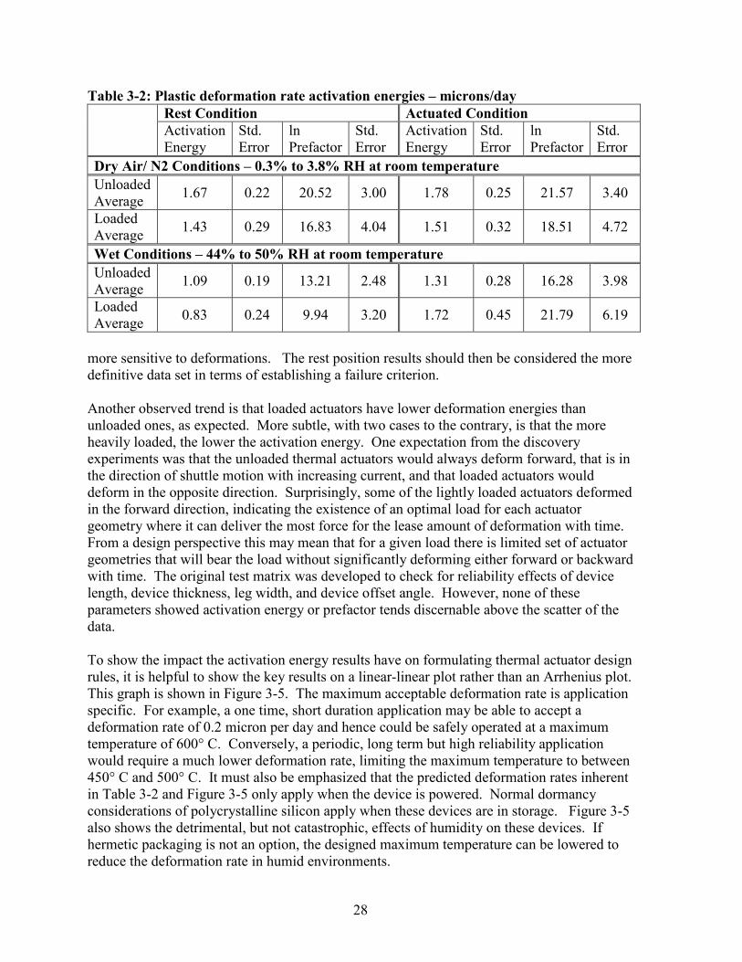
For clarity, Table 3-2 shows the activation energies and prefactors (and their associated

standard errors) averaged across all the device geometries, only making distinctions among

the environmental conditions and on whether the device was loaded or unloaded.

The rest condition energies are calculated from data collected after the actuator was allowed

to return to its rest position while the actuated condition results come from damage data

collected while the device was powered. We would expect these deformation activation

energies to be basically the same for the same device geometry and environmental

conditions. But there is a small trend in the dry data and a more noticeable trend in the wet

data that most of the rest position activation energies are lower than the hot activation

energies, even considering the ~20% standard errors in the activation energy values

themselves. One possible explanation is that while the deformation is essentially the same in

both cases, the device is closer to the end of its possible range of motion when powered. As

such, the additional deflection caused by the deformation is less and will lead to a smaller

absolute deformation rate than in the cold case. Hence the cold data would be marginally

28

more sensitive to deformations. The rest position results should then be considered the more

definitive data set in terms of establishing a failure criterion.

Another observed trend is that loaded actuators have lower deformation energies than

unloaded ones, as expected. More subtle, with two cases to the contrary, is that the more

heavily loaded, the lower the activation energy. One expectation from the discovery

experiments was that the unloaded thermal actuators would always deform forward, that is in

the direction of shuttle motion with increasing current, and that loaded actuators would

deform in the opposite direction. Surprisingly, some of the lightly loaded actuators deformed

in the forward direction, indicating the existence of an optimal load for each actuator

geometry where it can deliver the most force for the lease amount of deformation with time.

From a design perspective this may mean that for a given load there is limited set of actuator

geometries that will bear the load without significantly deforming either forward or backward

with time. The original test matrix was developed to check for reliability effects of device

length, device thickness, leg width, and device offset angle. However, none of these

parameters showed activation energy or prefactor tends discernable above the scatter of the

data.

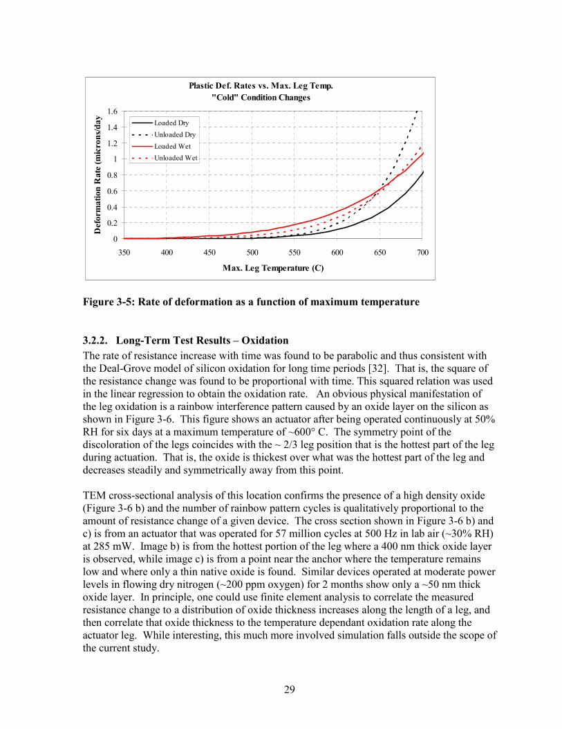
To show the impact the activation energy results have on formulating thermal actuator design

rules, it is helpful to show the key results on a linear-linear plot rather than an Arrhenius plot.

This graph is shown in Figure 3-5. The maximum acceptable deformation rate is application

specific. For example, a one time, short duration application may be able to accept a

deformation rate of 0.2 micron per day and hence could be safely operated at a maximum

temperature of 600° C. Conversely, a periodic, long term but high reliability application

would require a much lower deformation rate, limiting the maximum temperature to between

450° C and 500° C. It must also be emphasized that the predicted deformation rates inherent

in Table 3-2 and Figure 3-5 only apply when the device is powered. Normal dormancy

considerations of polycrystalline silicon apply when these devices are in storage. Figure 3-5

also shows the detrimental, but not catastrophic, effects of humidity on these devices. If

hermetic packaging is not an option, the designed maximum temperature can be lowered to

reduce the deformation rate in humid environments.

Table 3-2: Plastic deformation rate activation energies – microns/day

Rest Condition Actuated Condition

Activation

Energy

Std.

Error

ln

Prefactor

Std.

Error

Activation

Energy

Std.

Error

ln

Prefactor

Std.

Error

Dry Air/ N2 Conditions – 0.3% to 3.8% RH at room temperature

Unloaded

Average 1.67 0.22 20.52 3.00 1.78 0.25 21.57 3.40

Loaded

Average 1.43 0.29 16.83 4.04 1.51 0.32 18.51 4.72

Wet Conditions – 44% to 50% RH at room temperature

Unloaded

Average 1.09 0.19 13.21 2.48 1.31 0.28 16.28 3.98

Loaded

Average 0.83 0.24 9.94 3.20 1.72 0.45 21.79 6.19

29

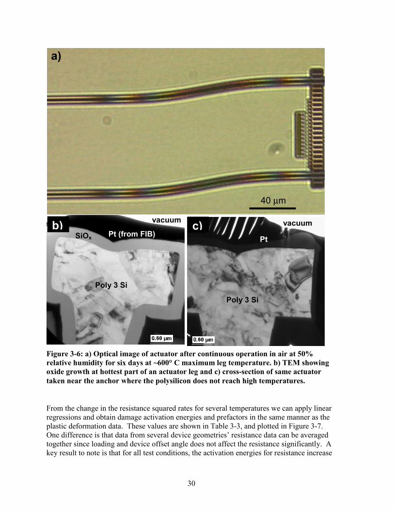
3.2.2. Long-Term Test Results – Oxidation

The rate of resistance increase with time was found to be parabolic and thus consistent with

the Deal-Grove model of silicon oxidation for long time periods [32]. That is, the square of

the resistance change was found to be proportional with time. This squared relation was used

in the linear regression to obtain the oxidation rate. An obvious physical manifestation of

the leg oxidation is a rainbow interference pattern caused by an oxide layer on the silicon as

shown in Figure 3-6. This figure shows an actuator after being operated continuously at 50%

RH for six days at a maximum temperature of ~600° C. The symmetry point of the

discoloration of the legs coincides with the ~ 2/3 leg position that is the hottest part of the leg

during actuation. That is, the oxide is thickest over what was the hottest part of the leg and

decreases steadily and symmetrically away from this point.

TEM cross-sectional analysis of this location confirms the presence of a high density oxide

(Figure 3-6 b) and the number of rainbow pattern cycles is qualitatively proportional to the

amount of resistance change of a given device. The cross section shown in Figure 3-6 b) and

c) is from an actuator that was operated for 57 million cycles at 500 Hz in lab air (~30% RH)

at 285 mW. Image b) is from the hottest portion of the leg where a 400 nm thick oxide layer

is observed, while image c) is from a point near the anchor where the temperature remains

low and where only a thin native oxide is found. Similar devices operated at moderate power

levels in flowing dry nitrogen (~200 ppm oxygen) for 2 months show only a ~50 nm thick

oxide layer. In principle, one could use finite element analysis to correlate the measured

resistance change to a distribution of oxide thickness increases along the length of a leg, and

then correlate that oxide thickness to the temperature dependant oxidation rate along the

actuator leg. While interesting, this much more involved simulation falls outside the scope of

the current study.

Figure 3-5: Rate of deformation as a function of maximum temperature

Plastic Def. Rates vs. Max. Leg Temp.

"Cold" Condition Changes

0

0.2

0.4

0.6

0.8

1

1.2

1.4

1.6

350 400 450 500 550 600 650 700

Max. Leg Temperature (C)

Deform

ation Rate (microns/day)

Loaded Dry

Unloaded Dry

Loaded Wet

Unloaded Wet

30

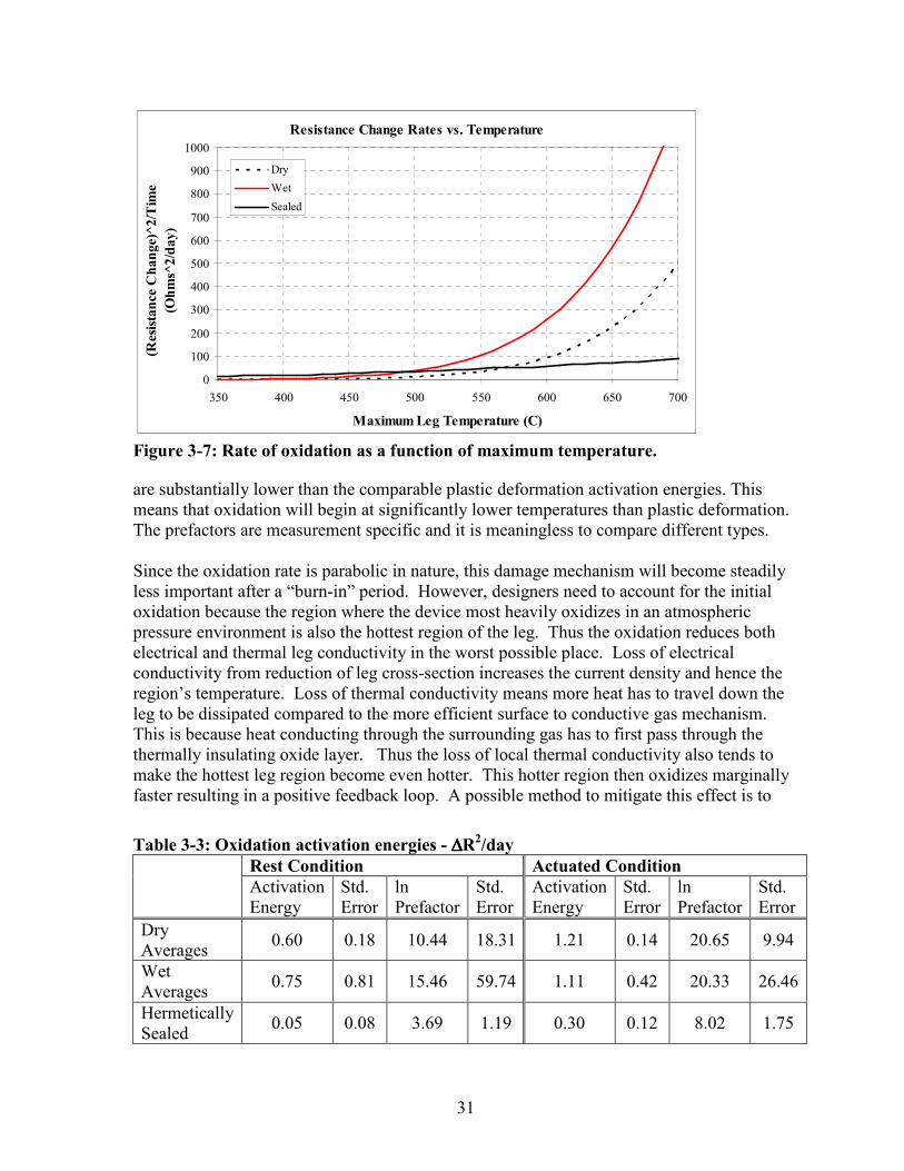
From the change in the resistance squared rates for several temperatures we can apply linear

regressions and obtain damage activation energies and prefactors in the same manner as the

plastic deformation data. These values are shown in Table 3-3, and plotted in Figure 3-7.

One difference is that data from several device geometries’ resistance data can be averaged

together since loading and device offset angle does not affect the resistance significantly. A

key result to note is that for all test conditions, the activation energies for resistance increase

.

Figure 3-6: a) Optical image of actuator after continuous operation in air at 50%

relative humidity for six days at ~600° C maximum leg temperature. b) TEM showing

oxide growth at hottest part of an actuator leg and c) cross-section of same actuator

taken near the anchor where the polysilicon does not reach high temperatures.

a)

40 µm

Poly 3 Si

SiOx Pt (from FIB)

vacuum b)

Pt

Poly 3 Si

vacuum c)

31

are substantially lower than the comparable plastic deformation activation energies. This

means that oxidation will begin at significantly lower temperatures than plastic deformation.

The prefactors are measurement specific and it is meaningless to compare different types.

Since the oxidation rate is parabolic in nature, this damage mechanism will become steadily

less important after a “burn-in” period. However, designers need to account for the initial

oxidation because the region where the device most heavily oxidizes in an atmospheric

pressure environment is also the hottest region of the leg. Thus the oxidation reduces both

electrical and thermal leg conductivity in the worst possible place. Loss of electrical

conductivity from reduction of leg cross-section increases the current density and hence the

region’s temperature. Loss of thermal conductivity means more heat has to travel down the

leg to be dissipated compared to the more efficient surface to conductive gas mechanism.

This is because heat conducting through the surrounding gas has to first pass through the

thermally insulating oxide layer. Thus the loss of local thermal conductivity also tends to

make the hottest leg region become even hotter. This hotter region then oxidizes marginally

faster resulting in a positive feedback loop. A possible method to mitigate this effect is to

Table 3-3: Oxidation activation energies - ∆∆∆∆R2/day

Rest Condition Actuated Condition

Activation

Energy

Std.

Error

ln

Prefactor

Std.

Error

Activation

Energy

Std.

Error

ln

Prefactor

Std.

Error

Dry

Averages 0.60 0.18 10.44 18.31 1.21 0.14 20.65 9.94

Wet

Averages 0.75 0.81 15.46 59.74 1.11 0.42 20.33 26.46

Hermetically

Sealed 0.05 0.08 3.69 1.19 0.30 0.12 8.02 1.75

Figure 3-7: Rate of oxidation as a function of maximum temperature.

Resistance Change Rates vs. Temperature

0

100

200

300

400

500

600

700

800

900

1000

350 400 450 500 550 600 650 700

Maximum Leg Temperature (C)

(Resistance Change)^2/Tim

e

(Ohms^2/day)

Dry

Wet

Sealed

32

vary the width of the leg along its length in a way that balances shuttle displacement / force

output with a more even temperature distribution along the leg. In other words, make the

hottest region of the leg wider or thicker.

Hermetic packaging is of only limited value in stopping initial resistance changes, but it does

effectively shut down all long term oxidation. Table 3-3 shows that hermetic packaging cuts

the oxidation ln(prefactors) by over 50%, which effectively shuts the oxidation down. While

package and chemical analysis of these parts still needs to be done, we suspect the oxygen

source for the initial oxidation is thermally induced redistribution of oxygen within the

package. That is, the hot thermal actuator legs act as a getter for any physisorbed oxygen in

the package and some chemisorbed oxygen on the device itself.

As expected, devices with the smallest leg cross-sections consistently showed the largest

resistance increases, those with the largest cross-sections had resistance changes barely

detectable about the data noise caused by 2-point contact resistance fluctuations. Errors in

the final resistance change activation energy values were much worse for the “cold” data sets

compared to the hot ones because the “on” state effective resistances were roughly twice as

large as the “off” state resistances and the contact resistances had a proportionately smaller

effect. (Most of the “cold – wet” resistance change data set was unusable for this reason.) In

retrospect, the devices should have been designed and wire bonded to allow for four-point

resistance measurements.

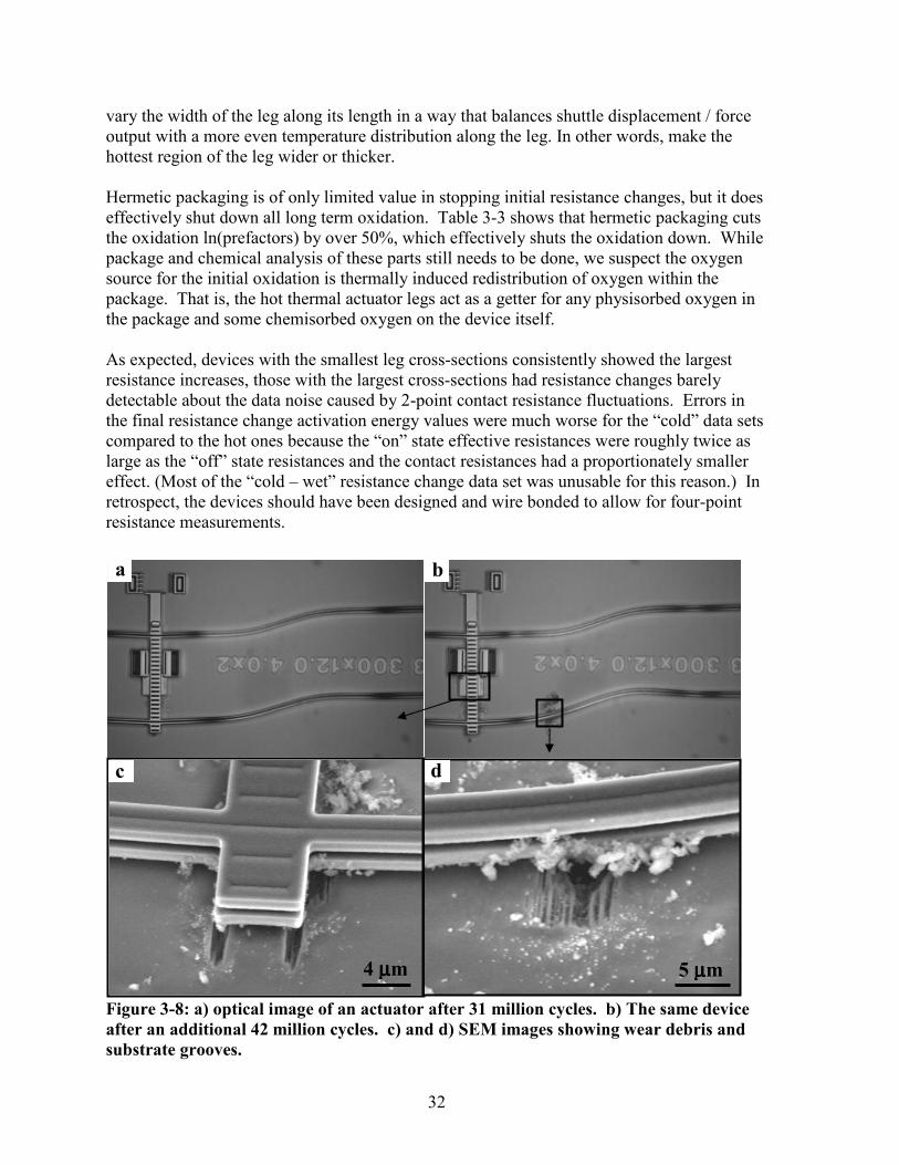
Figure 3-8: a) optical image of an actuator after 31 million cycles. b) The same device

after an additional 42 million cycles. c) and d) SEM images showing wear debris and

substrate grooves.

a b

c d

5 µµµµm 4 µµµµm

33

3.2.3. Cycling Experiments

The short term high power discovery experiments showed thermal actuators can generate a

significant amount of wear debris when modulated at high power levels for modest numbers

of cycles, as is shown in Figure 3-8. The device as shown in Figure 3-8 a) has been cycled at

270 mW for 31 million cycles in air and has clearly plastically deformed. Wear debris is

observed around the shuttle. Image b) shows the actuator after an additional 42 million

cycles, and during this time apparently some foreign object got stuck to a hot portion of the

lower right actuator leg and proceeded to generate significantly more wear debris (there are

no antistiction dimples under the actuator legs). The light colored region in a) and b) is the

visible glow of the device from Joule heating, giving an indication as to the temperature of

the legs. It is important to note that this is well above the normal operating temperature for

an actuator, as evidenced by the large plastic deformation visible in the images. The extent

of the wear trenches under the shuttle and the actuator leg are shown in SEM micrographs c)

and d) respectively. While actuators may not initially be affected by the wear debris they

generate, the debris can migrate to other MEMS devices and impact system level reliability.

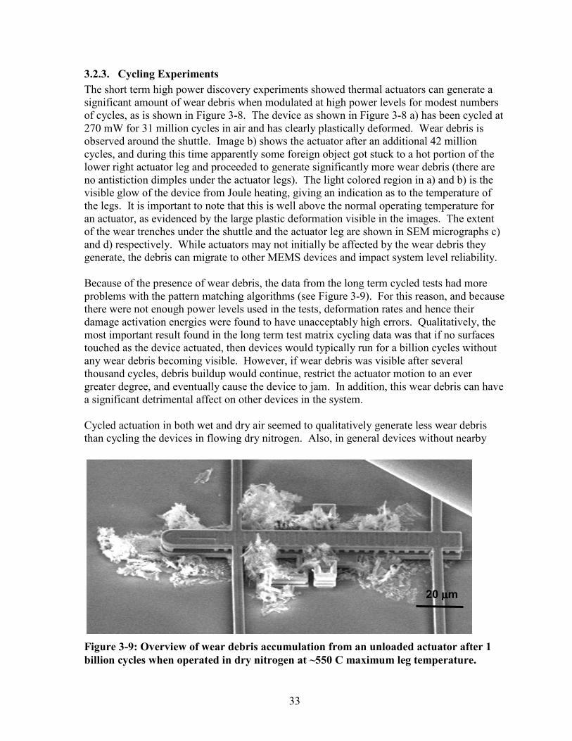
Because of the presence of wear debris, the data from the long term cycled tests had more

problems with the pattern matching algorithms (see Figure 3-9). For this reason, and because

there were not enough power levels used in the tests, deformation rates and hence their

damage activation energies were found to have unacceptably high errors. Qualitatively, the

most important result found in the long term test matrix cycling data was that if no surfaces

touched as the device actuated, then devices would typically run for a billion cycles without

any wear debris becoming visible. However, if wear debris was visible after several

thousand cycles, debris buildup would continue, restrict the actuator motion to an ever

greater degree, and eventually cause the device to jam. In addition, this wear debris can have

a significant detrimental affect on other devices in the system.

Cycled actuation in both wet and dry air seemed to qualitatively generate less wear debris

than cycling the devices in flowing dry nitrogen. Also, in general devices without nearby

Figure 3-9: Overview of wear debris accumulation from an unloaded a

billion cycles when operated in dry nitrogen at ~550 C maximum leg te

20 µµµµm

ctuator after 1

mperature.

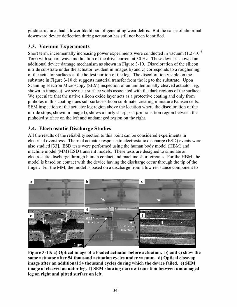
34

guide structures had a lower likelihood of generating wear debris. But the cause of abnormal

downward device deflection during actuation has still not been identified.

3.3. Vacuum Experiments

Short term, incrementally increasing power experiments were conducted in vacuum (1.2×10-6

Torr) with square wave modulation of the drive current at 30 Hz. These devices showed an

additional device damage mechanism as shown in Figure 3-10. Discoloration of the silicon

nitride substrate under the actuator, evident in images b) and c) corresponds to a roughening

of the actuator surfaces at the hottest portion of the leg. The discoloration visible on the

substrate in Figure 3-10 d) suggests material transfer from the leg to the substrate. Upon

Scanning Electron Microscopy (SEM) inspection of an unintentionally cleaved actuator leg,

shown in image e), we see near surface voids associated with the dark regions of the surface.

We speculate that the native silicon oxide layer acts as a protective coating and only from

pinholes in this coating does sub-surface silicon sublimate, creating miniature Kunsen cells.

SEM inspection of the actuator leg region above the location where the discoloration of the

nitride stops, shown in image f), shows a fairly sharp, ~ 5 µm transition region between the

pinholed surface on the left and undamaged region on the right.

3.4. Electrostatic Discharge Studies

All the results of the reliability section to this point can be considered experiments in

electrical overstress. Thermal actuator response to electrostatic discharge (ESD) events were

also studied [33]. ESD tests were performed using the human body model (HBM) and

machine model (MM) ESD transient models. These tests are designed to simulate an

electrostatic discharge through human contact and machine short circuits. For the HBM, the

model is based on contact with the device having the discharge occur through the tip of the

finger. For the MM, the model is based on a discharge from a low resistance component to

Figure 3-10: a) Optical image of a loaded actuator before actuation. b) and c) show the

same actuator after 54 thousand actuation cycles under vacuum. d) Optical close-up

image after an additional 54 thousand cycles during which the device failed. e) SEM

image of cleaved actuator leg. f) SEM showing narrow transition between undamaged

leg on right and pitted surface on left.

2 µµµµm

SEM View

Direction

a

d

e

b c

f

SEM View

Direction

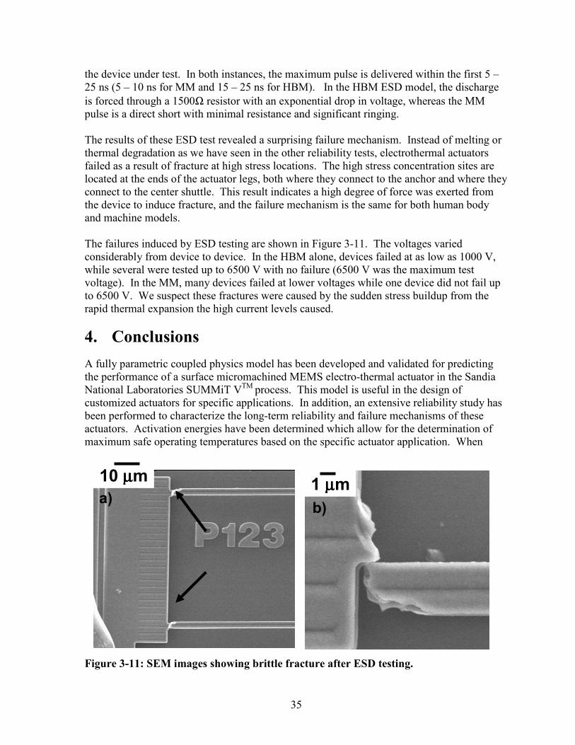
the device under test. In both instances, the maximum pulse is delivered within the first 5 –

25 ns (5 – 10 ns for MM and 15 – 25 ns for HBM). In the HBM ESD model, the discharge

is forced through a 1500Ω resistor with an exponential drop in voltage, whereas the MM

pulse is a direct short with minimal resistance and significant ringing.

The results of these ESD test revealed a surprising failure mechanism. Instead of melting or

thermal degradation as we have seen in the other reliability tests, electrothermal actuators

failed as a result of fracture at high stress locations. The high stress concentration sites are

located at the ends of the actuator legs, both where they connect to the anchor and where they

connect to the center shuttle. This result indicates a high degree of force was exerted from

the device to induce fracture, and the failure mechanism is the same for both human body

and machine models.

The failures induced by ESD testing are shown in Figure 3-11. The voltages varied

considerably from device to device. In the HBM alone, devices failed at as low as 1000 V,

while several were tested up to 6500 V with no failure (6500 V was the maximum test

voltage). In the MM, many devices failed at lower voltages while one device did not fail up

to 6500 V. We suspect these fractures were caused by the sudden stress buildup from the

rapid thermal expansion the high current levels caused.

4. Conclusions

A fully parametric coupled physics model has been developed and validated for predicting

the performance of a surface micromachined MEMS electro-thermal actuator in the Sandia

National Laboratories SUMMiT VTM

process. This model is useful in the design of

customized actuators for specific applications. In addition, an extensive reliability study has

been performed to characterize the long-term reliability and failure mechanisms of these

actuators. Activation energies have been determined which allow for the determination of

maximum safe operating temperatures based on the specific actuator application. When

Fi

10 µµµµm

35

gure 3-11: SEM images showing brittle fracture after ESD testing.

a) 1 µµµµm

b)

36

coupled with the validated modeling capabilities, this allows for reliability to be designed

into an actuator from the beginning.

4.1. Future work

Accurate material properties are critical in achieving an accurate model solution. A better

understanding of the various material properties affecting model accuracy is therefore

important. Specifically, values for thermal conductivity and the coefficient of thermal

expansion for SUMMiT polysilicon could be validated, as they are currently based on values

reported in the literature.

The physical cause behind the downward deflection of these devices still needs to be

determined. In all of the reliability and model validation work we have been unable to

determine the root cause of the downward motion, or even to determine trends in when it

does or does not occur. Elimination of this effect should drastically reduce the amount of

wear debris generation seen in this study.

Direct quantification of the plastic deformation of the actuator legs would be a more

accurate, complete approach to improve on the shuttle displacement based results presented

here. Likewise, four point probe measurements of the device effective resistances should

improve the accuracy of the oxidation activation energies.

The performance and reliability of multiple stage thermal actuators still needs to be

addressed. The model has been developed to include these designs, but it has not yet been

validated.

5. References

[1] J.H. Comtois, M.A. Michalicek, and C.C. Barron, “Electrothermal actuators fabricated

in four-level planarized surface micromachined polycrystalline silicon,” Sensors and

Actuators A, Vol. 70, pp. 23-31, 1998.

[2] Q.A. Huang and N.K.S. Lee, “Analysis and Design of Polysilicon Thermal Flexure

Actuator,” Journal of Micromechanics and Microengineering, Vol. 9, pp. 64-70, 1999.

[3] J.H. Comtois and V. M Bright, “Applications for surface-micromachined polysilicon

thermal actuators and arrays,” Sensors and Actuators A, Vol. 58, pp. 19-25, 1997.

[4] J.H. Comtois, M.A. Michalicek and C.C. Barron, “Characterization of electrothermal

actuators and arrays fabricated in a four-level, planarized surface-micromachined

polycrystalline silicon process,” 1997 International Conference on Solid-State Sensors

and Actuators, pp. 769-772, Chicago, June 16-19, 1997.

[5] L.Que, J.-S. Park and Y.B. Gianchandani, "Bent-Beam Electro-Thermal Actuators for

High Force Applications," IEEE Conf. on Micro Electro Mechanical Systems, Orlando,

Florida. pp. 31-36, Jan., 1999.

[6] L.L. Howell and S.M. Lyon, “Thermomechanical In-Plane Microactuator (TIM),” U.S.

Patent No. 6,734,597, issued May 11, 2004.

[7] R. Cragun and L.L. Howell, “Linear Thermomechanical Microactuators,”

Microelctromechanical Systems (MEMS), at the 1999 ASME International Mechanical

Engineering Congress and Exposition, pp. 181-188, November, 1999.

37

[8] L.Que, J.S. Park, Y.B. Gianchandani, "Bent-beam electrothermal actuators - Part I:

Single beam and cascaded devices," Journal of Microelectromechanical Systems, 10

(2), pp. 247-254, 2001.

[9] J.S. Park, L.L. Chu, A.D. Oliver, Y.B. Gianchandani, "Bent Beam Electrothermal

Actuators - Part II: Linear and rotary microengines," Journal of

Microelectromechanical systems, 10 (2), pp. 255-262, 2001.

[10] C.D. Lott, T.W. McLain, J.N. Harb and L.L. Howell, "Modeling the thermal behavior

of a surface-micromachined linear-displacement thermomechanical microactuator,"

Sensors and Actuators A, Vol. 101, pp. 239-250, 2002.

[11] J.T. Butler, V.M. Bright and W.D. Cowan, “Average Power Control and Positioning of

Polysilicon Thermal Actuators,” Sensors and Actuators A, Vol. 72, pp. 88-97, 1999.

[12] Q.A. Huang and N.K.S. Lee, “Analysis and Design of Polysilicon Thermal Flexure

Actuator,” Journal of Micromechanics and Microengineering, Vol. 9, pp. 64-70, 1999.

[13] J.J. Sniegowski and M.P. de Boer, “IC-compatible polysililcon surface

micromachining,” Annu. Rev. Mater. Sci., vol. 30, pp. 299-333, 2000.

[14] B.D. Jensen, M.P. de Boer, N.D. Masters, F Bitsie and D.A. LaVan, “Interferometry of

Actuated Microcantilevers to Determine Material Properties and Test Structure

Nonidealities in MEMS,” Journal of Microelectromechanical Systems, Vol. 10, No. 3,

pp. 336-346, September, 2001.

[15] L.J. van der Pauw, “A Method of Measuring the Resistivity and Hall Coefficient on

Lamellae of Arbitrary Shape,” Philips Tech. Rev., vol. 20, No. 8, p. 220-224, 1958.

[16] M.G. Buehler, S.D. Grant and W.R. Thurber, “Bridge and van der Pauw Sheet

Resistors for Characterizing the Line Width of Conducting Layers,” J. Electrochem.

Soc., vol. 125, no. 4, pp. 650-654, April, 1978.

[17] R.P. Manginell, “Polycrystalline-Silicon Microbridge Combustible Gas Sensor,” Ph.D.

Dissertation in Physics at the University of New Mexico, December, 1997.

[18] J.P. Holman, Heat Transfer, 8th Ed., McGraw-Hill, 1997.

[19] Y. Okada and Y. Tokumaru, “Precise determination of lattice parameter and thermal

expansion coefficient of silicon between 300 and 1500 K,” Journal of Applied Physics,

vol. 56, no. 2, pp. 314-320, 15 July 1984.

[20] H.G. Moore and A. Yaqub, A First Course in Linear Algebra with Applications, 3rd

edition, Academic Press, 1998.

[21] L.Lin and M. Chiao, “Electrothermal Responses of Lineshape Microstructures,”

Sensors and Actuators A, vol. 55, pp. 35-41, 1996.

[22] J.W. Wittwer, T.G. Gomm and L.L. Howell, “Surface micromachined force gauges:

uncertainty and reliability,” J. Micromech. Microeng., vol. 12, pp. 1-8, 2002.

[23] T.R. Hart, R.L. Aggarwal and B.Lax, “Temperature Dependence of Raman Scattering

in Silicon,” Physical Review B, vol. 1, no. 2, 15 Jan, 1970.

[24] H. Richter, Z.P. Wang and L. Ley, “The one phonon raman spectrum in

microcrystalline silicon,” Solid State Communications, vol. 39, pp. 625-629, 1981.

[25] G. Viera, S. Huet and L. Boufendi, “Crystal size and temperature measurements in

nanostructured silicon using Raman spectroscopy,” Journal of Applied Physics, vol.

90, no. 8, pp. 4175-4183, 15 October, 2001.

[26] L. Que, J.-S. Park and Y.B. Gianchandani, "Reliability Studies of Bent-Beam Electro-

Thermal Actuators," Reliability Physics Symposium. Proceedings Annual. IEEE

International Meeting, pp. 118-122, April 10, 2000.

38

[27] L. Que, L. Otradovec, A.D. Oliver and Y.B. Gianchandani, “Pulse and DC operation

lifetimes of bent-beam electrothermal actuators,” Technical digest, MEMS2001, 14th

IEEE International Conference on Microelectromechanical Systems, pp. 570-573,

Interlaken, Switzerland, 21-25 Jan., 2001.

[28] D.M. Tanner, N.F. Smith, D.J. Bowman, W.P. Eaton and K.A. Peterson, “First

Reliability Test of a Surface Micromachined Microengine Using SHiMMeR,” SPIE’s

1997 Symposium on Micromachining and Microfabrication, Austin, TX, pp. 14-23,

1997.

[29] N.F. Smith, W.P. Eaton, D.M. Tanner, J.J. Allen, “Development of characterization

tools for reliability testing of MicroElectroMechanical system actuators,” SPIE, vol.

3880, pp. 156-164, 1999.

[30] A. D. Corwin, and M. P. de Boer, “Scripting software for MEMS actuation and

automation”, to be published.

[31] L.L. Chu, D. Nelson, A.D. Oliver and Y.B. Gianchandani, “Performance enhancement

of polysilicon electrothermal microactuators by localized self-annealing,” IEEE

Sixteenth Annual International Conference on Microelectromechanical Systems,

Kyoto, Japan, pp. 68-71, 19-23 Jan, 2003.

[32] B.E. Deal and A.S. Grove, “General Relationship for Thermal Oxidation of Silicon,”

Journal of Applied Physics, vol. 36, no. 12, pp. 3770, 1965.

[33] J.A. Walraven, R.A. Plass, M.S. Baker and M.J Shaw, “Failure Analysis of

Electrothermal Actuators Subjected to Electrical Overstress (EOS) and Electrostatic

Discharge (ESD),” Submitted to International Symposium for Testing and Failure

Analysis, Worchester, MA, Nov. 14-17, 2004.

6. Distribution List

Copies Mail Stop Recipient Organization

1 1080 David Sandison 1769

1 1310 Michael Baker 1769

1 1310 Richard Plass 1762

1 1411 Thomas Headley 1822

1 1081 Jeremy Walraven 1739

1 1310 Fred Sexton 1762

1 1310 C Channy Wong 9113

1 1310 Steven Kempka 9113

1 0834 Sean Kearney 9112

1 1310 Leslie Phinney 9112

1 9154 Steven Gianoulakis 8774

1 0123 Donna Chavez 1011

1 9018 Central Technical Files 8945-1

2 0899 Technical Library 9616