FINAL REPORT CE

SCIENCE

United StatesEnvironmental ProtectionAgency

EPA/600/R-08/127 | December 2008 | www.epa.gov/ord

Emissions Test Report: Source Sampling for Transportable Gasifier for Animal Carcasses and Contaminated Plant MaterialFINAL REPORT

Office of Research and DevelopmentNational Homeland Security Research Center

ii

This page intentionally left blank.

EPA/600/R-08/127 | December 2008 | www.epa.gov/ord

Emissions Test Report: Source Sampling for Transportable Gasifier for Animal Carcasses and Contaminated Plant MaterialFINAL REPORT

Prepared by

Paul Lemieux U.S. Environmental Protection Agency Office of Research and Development National Homeland Security Research Center

Prepared for

U.S. Environmental Protection Agency Office of Research and Development National Homeland Security Research Center Research Triangle Park, NC 27711

U.S. Department of Agriculture Animal and Plant Health Inspection Services 4700 River Road Riverdale, MD 20737

U.S. Department of Defense Technical Support Working Group 201 12th St. South, Suite 300 Arlington, VA 22202

Office of Research and DevelopmentNational Homeland Security Research Center, Decontamination and Consequence Management Division

iv

AbstractThe U.S. Department of Defense (DoD) operates the Technical Support Working Group (TSWG) under a multi-agency program that provides information and technology development to support the needs of various U.S. government agencies to address counterterrorism and emergency response issues. TSWG, in collaboration with the U.S. Environmental Protection Agency’s National Homeland Security Research Center (EPA/NHSRC) and the U.S. Department of Agriculture’s Animal and Plant Health Inspection Service (USDA/APHIS) has funded the construction of a transportable gasifier with the goal of processing large quantities of animal carcasses and plant materials resulting from agricultural emergency events. This unit may be useful for other homeland security-related events as an on-site treatment/disposal process. This gasifier converts the biomass material into an inert ash and a combustible synthesis gas that is burned in a secondary combustion chamber. Temperatures within the unit nominally ranged from 1200 to 1800 °F (649 to 982 ºC).

This report describes an emissions test to characterize gasifier operation for the following reasons:

• To provide a basis for comparison with other combustion devices;

• To address public concerns about environmental impacts from carcass disposal operations;

• To give state and local environmental agencies information to support their responsibilities in siting and operating combustion equipment; and

• To allow the permanent siting of such devices at industrial settings in the agricultural industry (e.g., at rendering plants) for use with routine mortalities and for energy production.

Testing occurred during the period from March 3 to 6, 2008, at the Valley Protein rendering facility located in Rose Hill, NC. During these tests, the gasifier was operated on two different biomass feedstocks:

• A mixture of poultry and swine; and

• Bales of wheat straw.

Samples were taken and analyzed for several targets, including:

• Fixed combustion gases, including oxygen, carbon dioxide, carbon monoxide, total hydrocarbons, sulfur dioxide, and oxides of nitrogen;

• Particulate matter, including total filterable particulate, condensable particulates, PM10, and particle size distributions;

• Metals;

• Acid gases;

• Polychlorinated dibenzo-p-dioxins and polychlorinated dibenzofurans;

• Leachable metals in the ash residues; and

• Amino acids in the ash residues.

The unit was successfully deployed in the field in a rapid manner and was operational to perform the necessary emissions testing described in the Quality Assurance Project Plan in spite of having less than a week for initial startup and shakedown. This truncated shakedown schedule resulted in several operational issues that should be addressed through minor design modifications. The operational issues of concern that impacted the emissions testing included:

• Failure of the ash removal auger contributed to a limitation on feed rate;

• Inefficient distribution of macerated animal matter on the hearths in the primary chamber limited the unit’s maximum throughput to approximately 32% of the design capacity; and

• The plant material selected as a surrogate for contaminated plant matter could not be fed through the unit’s macerator; operations involving plant matter were therefore cut to only a few hours and extractive sampling was not performed on the plant matter test emissions.

Air was infiltrating the primary chambers through some unknown mechanism, and the synthesis gas as analyzed did not bear a resemblance to synthesis gas from other gasification processes – this difference could result from air migrating from the secondary chambers through gaps in the hearth to the primary chamber in the vicinity of the sampling port, turbulent mixing from the burner zones, or an overabundance of air pulled into the combustion unit through the ports in the doors.

Emissions of the measured pollutants were at very low levels, and the ash passed the Toxicity Characteristic Leaching Procedure (TCLP) test. The particle size distribution suggested that the vast majority of the emitted particulate matter was smaller than 0.5 microns.

A very important observation was that the emissions of carbon monoxide and total hydrocarbons correlated very well with the average temperatures of the two primary chambers. This observation suggests that for emergency response deployment, the primary chamber temperatures could be used as a surrogate monitoring parameter to ensure minimization of emissions.

Analysis of amino acid in the ash yielded non-detects for all target analytes. This observation indicates that the gasifier unit would be capable of destroying prions that could potentially cause Transmissible Spongiform Encephalopathy (TSE).

v

DisclaimerThe U.S. Environmental Protection Agency through its Office of Research and Development partially funded and collaborated in the research described herein under EP-C-04-023 with ARCADIS G&M. This report has been subject

to an administrative review but does not necessarily reflect the views of the Agency. No official endorsement should be inferred. EPA does not endorse the purchase or sale of any commercial products or services.

vi

Table of ContentsAcronyms and Abbreviations ......................................................................................................................................xiAcknowledgments ..................................................................................................................................................... xiii1.0 Introduction .............................................................................................................................................................12.0 Experimental ...........................................................................................................................................................3

2.1 Gasifier Description ..............................................................................................................................................3

2.1.1 Gasifier Construction Details .......................................................................................................................3

2.1.2 Refractory Materials and Trailer Mounting .................................................................................................3

2.1.3 Macerator .....................................................................................................................................................3

2.1.4 Feed System .................................................................................................................................................4

2.1.5 Stack .............................................................................................................................................................4

2.1.6 Auxiliary Fuel System..................................................................................................................................5

2.1.7 Ash Removal System ...................................................................................................................................5

2.2 Sampling and Analytical Methods ........................................................................................................................5

2.2.1 Measurement of Process Parameters ...........................................................................................................5

2.2.2 Sampling ......................................................................................................................................................8

3.0 Results ......................................................................................................................................................................93.1 Process Parameter Measurements ........................................................................................................................9

3.2 Continuous Emissions Monitors .........................................................................................................................17

3.2.1 Continuous Emissions Data from Test Day 1 (March 3, 2008) .................................................................17




3.2.5 Correlation of Operating Parameters .........................................................................................................28

3.3 Test Timeline and Average Concentrations ........................................................................................................28

3.4 Particulate Matter ...............................................................................................................................................31

3.4.1 Ambient Particulate ....................................................................................................................................31

3.4.2 Total Filterable Particulate .........................................................................................................................31

3.4.3 Filterable Particulate Matter and Condensable Particulate Matter ............................................................31

3.4.4 Visible Emissions .......................................................................................................................................32

3.4.5 Particle Size Distributions ..........................................................................................................................33

3.5 Hydrogen Chloride and Chlorine .......................................................................................................................33

3.6 Metals .................................................................................................................................................................34

3.7 PCDDs/Fs ...........................................................................................................................................................36

3.8 Synthesis Gas Composition ................................................................................................................................38

3.9 Ash Analysis .......................................................................................................................................................38

3.10 Estimated Emissions of Pollutants Per Mass of Carcass Fed ...........................................................................39

4.0 Quality Assurance/Quality Control Evaluation Report ....................................................................................414.1 CEMs (CO2/O2, SO2, NOx, CO, THCs) .............................................................................................................41

vii

Table of Contents4.2 HCl, Cl2 (Method 26/26A) .................................................................................................................................41

4.3 Filterable Particulate (Method 5) .......................................................................................................................41

4.4 PCDDs/PCDFs (EPA Method 23) ......................................................................................................................41

4.5 Metals (EPA Method 29) ....................................................................................................................................41

4.6 PM10, Condensable Particulate (EPA M201A/OTM-DIM) ................................................................................42

4.7 CO2, CH4, N2, O2, NMOC, CH4 in Synthesis Gas ..............................................................................................42

4.8 Total Suspended Particulate ................................................................................................................................42

4.9 Ash Composition (EPA Method 1311/TCLP) ....................................................................................................42

4.10 Ash Amino Acids ..............................................................................................................................................42

4.11 Data Quality Assessment (DQA) ......................................................................................................................42

5.0 Conclusions ............................................................................................................................................................436.0 References ..............................................................................................................................................................45

viii

List of Figures

Figure 2-1. Gasifier Concept Schematic (Courtesy BGP, Inc.) .......................................................................................3

Figure 2-2. Cross-sectional View of Gasifier from the Front .........................................................................................3

Figure 2-3. Trailer Mounted Transportable Gasifier Schematic (Courtesy BGP, Inc.) ...................................................3

Figure 2-4. Macerator .....................................................................................................................................................4

Figure 2-5. Feed Distribution System .............................................................................................................................4

Figure 2-6. Feeding Animal Carcasses into Macerator ...................................................................................................4

Figure 2-7. Telescoping Stack .........................................................................................................................................4

Figure 2-8. Stack Dilution Inlet ......................................................................................................................................5

Figure 2-9. Cross-sectional View of Hearth and Ash Removal Auger ...........................................................................5

Figure 2-10. Temperature Readouts ................................................................................................................................7

Figure 2-11. Dimensions of Broom and 500-gallon Fuel Tank. .....................................................................................7

Figure 2-12. Geometric Construction of 500-gallon. Fuel Tank. ....................................................................................7

Figure 2-13. Stack Side View .........................................................................................................................................8

Figure 3-1. Average Carcass Feed Rate ........................................................................................................................17

Figure 3-2. Stack O2 and CO2 from Test Day 1 ............................................................................................................18

Figure 3-3. SC O2 and CO2 from Test Day 1 ................................................................................................................18

Figure 3-4. Stack CO and THC from Test Day 1 ..........................................................................................................18

Figure 3-5. Stack NOx and SO2 from Test Day 1 ..........................................................................................................19

Figure 3-6. Temperatures from Test Day 1 ...................................................................................................................19

Figure 3-7. Dilution Ratio from Test Day 1 (Average = 2.36) ......................................................................................19

Figure 3-7. Dilution Ratio from Test Day 1 (Average = 2.36) ......................................................................................20

Figure 3-8. Stack O2 and CO2 from Test Day 2 ............................................................................................................20

Figure 3-9. SC O2 and CO2 from Test Day 2 ................................................................................................................21

Figure 3-10. Stack CO and THC from Test Day 2 ........................................................................................................21

Figure 3-11. Stack NOx and SO2 from Test Day 2 ........................................................................................................21

Figure 3-12. Temperatures from Test Day 2 .................................................................................................................22

Figure 3-13. Dilution Ratio from Test Day 2 (Average = 2.34) ....................................................................................22

Figure 3-14. Stack O2 and CO2 from Test Day 3 ..........................................................................................................23

Figure 3-15. SC O2 and CO2 from Test Day 3 ..............................................................................................................23


Figure 3-17. SC CO from Test Day 3 ...........................................................................................................................24




Figure 3-21. Stack O2 and CO2 from Test Day 4 ..........................................................................................................26

Figure 3-22. SC O2 and CO2 from Test Day 4 ..............................................................................................................26



ix



Figure 3-27. PC Temperature vs. CO ............................................................................................................................28

Figure 3-28. PC Temperature vs. THC .........................................................................................................................28

Figure 3-29. Particle Size Distribution .........................................................................................................................33

x

List of Tables

Table 2-1. Table of Sampling Activities ..........................................................................................................................6

Table 3-1. Fuel Consumption Results .............................................................................................................................9

Table 3-2. Temperature and Set Point Data from Test Day 1 .......................................................................................10




Table 3-5. Temperature and Set Point Data from Test Day 4 (Continued) ...................................................................14

Table 3-5. Temperature and Set Point Data from Test Day 4 (Continued) ...................................................................15

Table 3-6. Estimated Feed Quantities and Times ..........................................................................................................16

Table 3-7. Sample Train Start/Stop Times and Average Stack Gas Concentrations, Dry Basis ...................................29

Table 3-8. CEM Average Measurements, Dry Basis ....................................................................................................30

Table 3-9. Stack Velocities and Flow Rates ..................................................................................................................30

Table 3-10. Ambient PM10 Results ................................................................................................................................31

Table 3-11. Total Filterable Particulate Results ............................................................................................................31

Table 3-12. Particulate Matter Emissions Measurements .............................................................................................32

Table 3-13. Visible Emissions During Vegetable Matter Tests (Day 4) ........................................................................32

Table 3-14. Particle Size Distribution Data (Mass Basis) .............................................................................................33

Table 3-15. Hydrogen Chloride and Chlorine ...............................................................................................................34

Table 3-16. Metals Results ............................................................................................................................................35

Table 3-17. PCDD/F Concentrations (pg/Nm3) ............................................................................................................36

Table 3-18. PCDD/F Mass Emission Rate (lb/hr) ........................................................................................................37

Table 3-19. Synthesis Gas Composition .......................................................................................................................38

Table 3-20. TCLP Results for Ash (mg/L) ....................................................................................................................38

Table 3-21. Amino Acid Analytical Results for Ash (mg/g) .........................................................................................39

Table 3-22. Estimated Emissions ..................................................................................................................................40

xi

Acronyms and Abbreviations

APHIS Animal and Plant Health Inspection ServiceCAA Clean Air ActCCB(s) continuing calibration blank(s)CCV(s) continuing calibration verification(s)CEM(s) continuous emission monitor(s)COTS commercial off-the-shelfCDI ambient O2 concentrationCi concentration of pollutant i in ppmCSC secondary chamber concentrationCST stack concentrationCVAA cold vapor atomic absorption spectrophotometryDoD U.S. Department of DefenseDQA data quality assessmentDR dilution ratioDSCF dry standard cubic foot (feet)DSCM dry standard cubic meter(s)EMSL Environmental Monitoring Systems LaboratoryEPA U.S. Environmental Protection Agencyg gram(s) gal gallon(s)GFAA graphite furnace atomic absorption spectrophotometryµg microgram(s)HPLC high performance liquid chromatographyhr hour(s)HpCDD heptachlorodibenzo-p-dioxinHpCDF heptachlorodibenzofuranHxCDD hexachlorodibenzo-p-dioxinHxCDF hexachlorodibenzofuranICP inductively coupled plasma optical emission spectrometryICV(s) initial calibration verification(s)lb pound(s)LED light emitting diodem meter(s)µm micrometer(s)mg milligram(s)Mi molecular mass of pollutant imin minute(s)MQO(s) Measurement Quality Objective(s)Nm3 normal cubic meter(s)NOx oxides of nitrogenNPT nominal pipe threadNSPS New Source Performance Standard(s)OCDD octachlorodibenzo-p-dioxinOTM-DIM Other Test Method – Dry Impinger Method

xii

PC primary chamberPCDD polychlorinated dibenzo-p-dioxinPCDF polychlorinated dibenzofuranPeCDF pentachlorodibenzofuranpg picogram(s) ppm parts per millionQDI dilution flowQS stack flow rateQSC secondary chamber flowQST stack flowNA not availableND not detectedNHSRC National Homeland Security Research CenterOCDF octachlorodibenzofuranPM10 Particle(s) with an aerodynamic diameter of 10 micrometers or lessPeCDD pentachlorodibenzo-p-dioxinQAPP Quality Assurance Project PlanR correlation coefficientR ideal gas constantRCRA Resource Conservation and Recovery ActSC secondary chamberSETA Systems Engineering and Technical Assistancet timeT temperatureTCDD tetrachlorodibenzo-p-dioxinTCDF tetrachlorodibenzofuranTCLP Toxicity Characteristic Leaching ProcedureTEF Toxicity Equivalency FactorTEQ Toxic EquivalencyTHC total hydrocarbon(s)TSE Transmissible Spongiform EncephalopathyTSWG Technical Support Working GroupUSDA U.S. Department of AgricultureWHO World Health Organization

xiii

Acknowledgments

The author would like to acknowledge John McKinney of TSWG SETA Support for his efforts on this project. Jim Howard of the North Carolina Department of Agriculture deserves special recognition for his efforts at making these tests happen. The author would also like to thank Yuanji Dong, Gene Stephenson, Michal Derlicki, Richard Snow,

and John Nash of ARCADIS for their work on the sampling and analysis portion of this report. Special thanks to C.W. Lee of EPA’s National Risk Management Research Laboratory, and Shannon Serre and Joe Wood of EPA’s National Homeland Security Research Center for their invaluable help and advice on this project.

xiv


1

1.0Introduction

The U.S. Department of Defense (DoD) operates the Technical Support Working Group (TSWG) under a multi-agency program that provides information and technology development to support the needs of various U.S. government agencies to address counterterrorism and emergency response issues. TSWG, in collaboration with the U.S. Environmental Protection Agency’s National Homeland Security Research Center (EPA/NHSRC) and the U.S. Department of Agriculture’s Animal and Plant Health Inspection Service (USDA/APHIS) has funded the construction of a transportable gasifier with the goal of processing large quantities of animal carcasses and plant materials resulting from agricultural emergency events. This unit may be useful for other homeland security-related events as an on-site treatment/disposal process. This gasifier converts the biomass material into an inert ash and a combustible synthesis gas that is burned in a secondary combustion chamber. Temperatures within the unit nominally ranged from 1200 to 1800 °F (649 to 982 ºC).

This report describes an emissions test to characterize gasifier operation for the following reasons:





Testing occurred during the period from March 3 to 6, 2008, at the Valley Protein rendering facility located in Rose Hill, NC. During these tests, the gasifier was operated by the manufacturer (BGP, Inc.) on two different biomass feedstocks:

• A mixture of poultry and swine; and

• Bales of wheat straw.

The initial plan was for poultry and swine to be tested separately. However, feed for the gasifier was acquired by diverting some of the trucks delivering dead stock to the test site to supply material for the gasifier, and the feed stock material dropped onto the concrete receiving pad could remain there no longer than 24 hours. It was therefore not feasible to have a single species of animal for the feed. In addition, due to the highly compressed shakedown schedule, the unit was not operating at full design capacity throughout the tests.

The complete effort involved:

(1) delivery and setup of the prototype gasifier at the test site for evaluation;

(2) delivery and installation of advanced shredding/grinding equipment (macerator) at the site;

(3) acquisition of feed materials for performance testing;

(4) startup and shakedown of the system, using a variety of feeds and operating conditions;

(5) establishment of operating parameters required for near-steady-state operation; and

(6) source sampling during gasifier operation according to an EPA-approved Quality Assurance Project Plan (QAPP) (ARCADIS, 2007). This emissions test report addresses the testing covered by the QAPP.

Samples were taken and analyzed for several targets including:



• Metals;

• Acid gases;

• Polychlorinated dibenzo-p-dioxins and polychlorinated dibenzofurans (PCDDs/Fs);



The overall program objective was to deliver a prototype gasifier capable of being transported over all primary and secondary roads, for this prototype gasifier to be capable of being operational in less than 24 hours after arrival at the site, and for this prototype gasifier to have the capability to process 25 tons per day of contaminated animal carcasses or plants.

The objective of these tests was to determine the emission rates and concentrations of the target constituents by sampling the exhaust from the combustion of the synthesis gas produced in the primary chambers of the prototype gasifier.

The resulting data will be utilized by the collaborating entities to determine the operational and environmental impacts of utilizing this gasifier to process different types of agricultural residues. Although there were additional variables of interest (e.g., impact of weather conditions, other feeds), available time and resources precluded including these additional variables as test parameters.

2


3

2.0 Experimental

2.1 Gasifier DescriptionThe BGP-D1000 gasifier is designed to process 25 tons per day of feed material, using a series of chambers, each with different fuel/air stoichiometry. Two independent primary chambers (PCs) operating sub-stoichiometrically feed into two independent secondary chambers (SCs), thus achieving a quasi-steady-state operating mode. Heat from the SCs provides the hearth with heat. The thermal inertia of the hearth prevents significant PC temperature loss when high water content materials are charged onto the hearth. The unit operates on natural draft without requiring an induced draft fan. Up to eight units can be manifolded together to achieve larger capacities, up to approximately 200 tons per day, comparable to other large capacity fixed-site technologies. Figure 2-1 shows a concept schematic diagram of the gasifier. Additional information can be found elsewhere (BGP, 2008).

Secondary Chamber

Feedstock

Primary Chamber

Stack

Feed

Figure 2-1. Gasifier Concept Schematic (Courtesy BGP, Inc.)

2.1.1 Gasifier Construction DetailsThe BGP-D1000 is prototyped to be compatible with a production model Commercial Off-The-Shelf (COTS) trailer. The prototype length is 27 feet, and the prototype height is 11 feet 5 inches, designed to create a total vehicle height of less than the 162-inch legal limit so that the unit can be transported on all primary and secondary roads in the United States. The width of the prototype is approximately 11 feet 2 inches. The materials selected for the prototype unit shell have been selected to accommodate a standard 35-ton capacity low-boy trailer, capable of transporting a total payload weight of approximately 60,000 pounds. Additionally, the two-chamber design allows for increased flexibility: the gasifier can also handle smaller loads; one PC/SC combination can be left dormant without significantly affecting the operating conditions in the other chambers or one chamber can dispose of one type of waste while the other chamber handles another type. Reducing or partially eliminating any cool-down of the gasifier will increase throughput. Alternate loading of the chambers can be utilized to minimize cool-down.

RefractoryLining

PC APC B

SC B SC ADuct

Transition Duct

Telescoping Stack

Hearth

Transition Duct

Oil Burners (2) Oil Burners (2)

Stack Gas

Feed

Figure 2-2. Cross-sectional View of Gasifier

from the Front 2.1.2 Refractory Materials and Trailer MountingThe refractory materials have been selected based on an assessment of the required transporting and operating conditions of the transportable unit. Ceramic fiber has been incorporated into this highly specialized refractory design, while maintaining refractory strength where required. Figure 2-3 shows a schematic of the gasifier as mounted on a trailer. The burners fire into each SC and the exhaust from the SCs enters the stack from a common breeching. Air is introduced into the PCs through small ports in the doors. No burners fire into the PCs, and all fumes from the PCs must pass through their respective SCs en route to the stack.

Figure 2-3. Trailer Mounted Transportable Gasifier Schematic (Courtesy BGP, Inc.)

2.1.3 MaceratorThe COTS macerator that was purchased has a throughput ranging from 60,000 to 100,000 lb/hr of the carcass of any domestic animal species up to approximately the size of pigs. Larger carcasses (e.g., cattle) require a pre-breaker prior to the macerator. The pre-breaker was not included in the purchase of the macerator for the prototype. Figure 2-4 shows the macerator, which is mounted on a second COTS

4

trailer. Material leaves the macerator as approximately 1-inch chunks, in a slurry similar to that leaving a meat grinder.

The macerator is sized so that several gasifier units can be manifolded into a single macerator, resulting in a technology that is scaleable for different-sized events.

2.1.4 Feed SystemGround material leaves the macerator and is pumped into a feed distribution system that drops the material through a straight pipe onto the hearth in the PCs through manually actuated high temperature gate valves (see Figure 2-5). The material drops onto the hearth via gravity and is intended to spread out over the entire surface area of the hearth. During the tests, the material did not spread very effectively. Instead, macerated material tended to make piles underneath the feed ports, and hearth coverage was estimated to be only on the order of 40%. The only way to achieve effective distribution of the material on the hearth was to open the front doors of the PCs and manually spread the material using a metal rake. This action disrupted the sub-stoichiometric operation of the gasifier, resulting in the below-design-capacity feed rates observed during the tests. The intermittent nature of these disruptions apparently did not significantly alter the overall stack gas flow rates and thus likely did not affect sample quality.

Figure 2-4. Macerator

Figure 2-5. Feed Distribution System

The unit was fed using a “bobcat” type front end loader with a nominal bucket capacity between 500 and 600 lb (based on operator experience). Materials were scooped off the ground and loaded into the macerator as shown in Figure 2-6.

Figure 2-6. Feeding Animal Carcasses into Macerator 2.1.5 StackThe gasifier unit is equipped with a 34-inch diameter and approximately 12-foot high telescoping stack (Figure 2-7) projecting above the gasifier, with a 34-inch diameter dilution air inlet at the base of the stack (Figure 2-8), which allows control of the natural draft that draws the air through the primary chambers and draws the combustion gases through the secondary combustion chambers. Sampling ports

Figure 2-7. Telescoping Stack

(and consequently stack measurements) would normally be located at least 8 stack diameters downstream of the dilution air inlet. However, the stack’s height is only 12 feet, which will not allow such sampling port placement. In this case, measurements were made at least 2 stack diameters downstream of the damper (visible inside the dilution duct on Figure 2-7). Since any particulate matter measurements at the stack must be corrected for background PM in the dilution air, it was necessary to characterize the flow rate and PM loading in the dilution air. A duct extension was therefore mounted on the dilution air inlet so that the dilution air flow rate could be measured at an appropriate distance from the air

5

entrance of the duct extension without entrance disturbance. NOTE: The flow rate through the dilution air inlet was too low to be measured using any of the gas flow measurement devices that were available to the sampling crew, so dilution air was estimated using the dilution ratio based on the stack and SC concentrations of oxygen and carbon dioxide. The PM concentration in the dilution air was quantified by a traditional ambient PM10 particulate sampler positioned near the dilution air duct inlet.

Figure 2-8. Stack Dilution Inlet 2.1.6 Auxiliary Fuel SystemFour burners (two were redundant) capable of each firing 8 gal/hr of No. 2 fuel oil were mounted in the duct between the primary and secondary chambers (i.e., two burners on each side). These burners provided initial heat to make the hearth hot enough to initiate gasification in the primary chambers. The burners also provided process control to maintain predetermined temperatures in the secondary chambers. Each burner was fed from a fuel tank mounted on the trailer. The burner fuel tanks were refilled from a 500-gallon fuel tank positioned at the rear end of the trailer. It was advantageous that each burner had a redundant duplicate, since two of the burners failed during shakedown due to overheating after a generator failure. This failure led to an important lesson about the need to be able to swap out and/or repair the burners while the unit was operating. The fuel in the tanks was analyzed by Standard Laboratories, Inc., and was found to be low in sulfur (0.02%) and nitrogen (0.01%) with < 0.001 % ash content.

Ash RemovalAuger

HearthFeed

Figure 2-9. Cross-sectional View of Hearth and Ash

Removal Auger

2.1.7 Ash Removal SystemThe gasifier unit was designed with a reservoir at the back end of the primary chamber to collect ash from the hearths (see Figure 2-9). An ash removal auger was supposed to periodically remove the ash to be collected in metal bins outside the gasifier. However, the ash removal auger was damaged during startup and did not work throughout the tests. There was no way to quantify the amount of ash produced in the process.

2.2 Sampling and Analytical MethodsSampling was performed over four test days during which the gasifier was operating under representative conditions as determined during a very brief period of shakedown testing.Extractive samples were taken for periods as specified in Table 2-1. Much of the monitoring instrumentation that was supposed to be installed by BGP was not available in the manner prescribed in the QAPP due to financial constraints and the compressed schedule. In particular, the following measurements that were specified in the QAPP were not available on the prototype:

• Feedstock feed rate and macerator pump indicator;

• Fuel oil flow rate;

• Burner and secondary air flow rate;

• Air flow rate to primary chamber; and

• Ash mass.

Wherever possible, alternate means for estimating these parameters were used and the methods are documented in this report. The most significant deficiency was the uncertainty in the feed weights. This uncertainty is likely to affect the overall estimated emissions calculations in Section 3.10. However, given that most emission factors published in the EPA’s AP-42 emission factor database [EPA, 1995] are typically order-of-magnitude estimates, these uncertainties are not likely to significantly change the interpretation of the test results.

2.2.1 Measurement of Process ParametersThe prototype unit was equipped with minimal process measurement instrumentation. Only the temperatures in the PCs and SCs were monitored, and the temperatures were only available via an LED readout (shown in Figure 2-10) on the control panel for each PC/SC combination. The temperatures from these readouts were manually recorded onto data sheets every 15 minutes, except when the vegetative matter was being fed, in which case the temperatures were manually recorded every 2 minutes.

6

Table 2-1. Table of Sampling Activities

Parameter LocationSampling/

Analytical MethodFrequency of

SamplingSampling Day

Feedstock feed rate Field

Visual estimation based on 550 lb/bucket on bobcat and bobcat operator experience

Each feed event All

Fuel oil flow rate 500-gal fuel tank DipstickEach time fuel added

or taken from tankAll

Oil fuel elemental composition (C, H, O, N, and S) and heating value

Fuel tankSupplied by vendor or

grab samplingOne sample Grab

Dilution air flow rate and temperature

Damper air duct EPA Methods 1 & 2NO DATA – FLOW TOO

LOW TO MEASUREAll

Stack flue gas flow rate and temperature

Stack EPA Methods 1 & 2Traverse during all

extractive testsAll

Temperatures Primary chamber Single point in each PC15 min (2 during vegetable matter)

All

Temperature Secondary chamber Single point in each SC15 min (2 during vegetable matter)

All

Ash composition Front door Periodic grab samplesOne per day

from each PCGrab

Diluted flue gas composition (O2, CO2, CO, NOx-, SO2, and THC)

StackCEM (EPA M3A, 10, 7E, 6C, 25A)

Continuous All

Flue gas prior to dilution (O2 and CO2)

Exit of SC CEM (EPA M3A) Continuous All

PM10 and condensable particulate StackEPA Methods 201A & 202

One sample per day 1, 2, 3

Total PM, HCl, and Cl2 Stack EPA Methods 5 & 26 Two samples per day 1, 2, 3

Dioxins/furans in flue gas Stack EPA Method 23 Two samples per day 1, 2, 3

Metals in flue gas Stack EPA Method 29 Two samples per day 1, 2, 3

PM10 in dilution air Ambient EPA HiVol One sample per day 1, 2, 3

PC Syngas composition (CO, CO2, H2, O2, H2O, CH4, and non-methane HC)

Primary chamber EPA M3C, 25CAt least one

sample per day1, 2, 3

Visible Emissions (Opacity) Stack EPA Method 9

Intermittently during carcass burns,

continuously during vegetative burns

1,2,3,4

7

Figure 2-10. Temperature Readouts

Feed rates were measured by estimation of the degree of fullness of the bucket in the front end loader shown in Figure 2-6. Based on operator experience, a full bucket contained between 500 and 600 lb of material, while a half bucket contained between 250 and 300 lb of material. Neither the large 500-gallon fuel tank that was used as a reservoir for the burner fuel tanks nor the burner fuel tanks had any sort of level indicator, sight glass, or flow measurement device. In order to measure fuel consumption rates, a broomstick was used as a dipstick in the large fuel tank. The measurements of the tank are shown in Figure 2-11. A discussion of procedures used to measure the fuel consumption rate follows.

Fuel Tank Level

Broom

Fill Cap Fitting

Fuel Tank

1.5 in.

L = Tank Length = 74.14 in.

B

X = B-1.5

46 in.

T = Tank Wall Thickness = .125 in.

Figure 2-11. Dimensions of Broom and 500-gallon Fuel Tank

A geometric construction of the tank was created. This construction is shown in Figure 2-12.

X

r

r sin

Figure 2-12. Geometric Construction of

500-gallon Fuel Tank Using this geometric construction,

(1) Cross-sectional area of tank = r2 (1)

(2) Area of slice of tank cut by angle

2θ= ( )πr2 ⎛ ⎞ 2θ ⎜ ⎟ = r θ 2

(2)⎝ π ⎠

The cross-sectional area of the equilateral triangle formed by two radii and the line formed by the fuel in the tank is defined as:

1Area⎛

Δ ⎟ (rsin (rcos ) = r2= 2⎞

⎜ 2

θ) θ sinθ cosθ (3)⎝ ⎠

The cross-sectional area of the liquid in the tank is calculated by subtracting Eq. (3) from Eq. (2):Area 2θ − r2

liquid = r sinθ cosθ (4)

The known quantity is X, the distance from the top of the tank to the liquid level in the tank. Thus:

r − ( )2r − X = rcosθ (5)

Therefore:

arccos⎛ X ⎞

θ = ⎜ 1r

− ⎟ (6)⎝ ⎠

A spreadsheet was used to calculate θ as a function of X using Eq. (6), and the values for were used in Eq. (4) to θestimate the cross-sectional area. The volume of the liquid was calculated by multiplying the cross-sectional area by the length of the tank (allowing for the 1/8" wall thickness of the tank).

8

StackCross-Section

Exhaust

Gasifier

Stack

Dilution AirDuct Extension

Dilution Air

2-inch NPT Sample Ports@ 90 Degree Pitch

5-inch NPT Sample Ports@ 90 Degree Pitch

2-inch Sample Port

Syngas from PC

Flue Gas from SCDilution Damper

Figure 2-13. Stack Side View

2.2.2 SamplingThe primary sampling location was the stack of the gasifier. The stack has a 34-inch inner diameter and an extended height of 12 feet. Two 5-inch diameter sampling ports were located at 90 degrees from each other and a third 2-inch port was located between the two. The location of the two 5-inch ports was determined according to the requirements described in the EPA sampling Methods 1 and 2 to increase the accuracy of the flow measurement. The two-inch port was installed to accommodate non-isokinetic sampling, e.g., CEMs and particle sizing. Figure 2-13 shows the configuration of these sampling ports. With the isokinetic sampling trains utilizing the two 5-inch nominal pipe thread (NPT) ports (e.g., metals, dioxin/furans), the stack was traversed to measure the variation in gas velocity over its cross-section by rotating the sampling trains between the ports. With the height of the trailer included, gasifier samples were taken at approximately 26–28 feet above the ground.

The secondary sampling location was the dilution air duct extension (as provided by the manufacturer). The extension had two 2-inch ports located 90 degrees apart to accommodate non-isokinetic sampling, e.g., CEMs and air flow rate determination. Unfortunately, the flow in this duct was too low in velocity to measure with the available equipment. An ambient total particulate sampler located near its inlet quantified the contribution of the dilution air to the stack particulate loading.

The target stack gas constituents and parameters of interest in this program are:

• PM10 particulate matter;

• Total particulate matter;

• Condensable particulate matter;

• RCRA/CAA metals (Sb, As, Ba, Be, Cd, Cr, Co, Pb, Mn, Hg, Ni, Se, Ag);

• HCl/Cl2;

• Dioxins/furans;

• CO2;

• O2;

• CO;

• NOx;

• SO2; and

• Total Hydrocarbons (THC).

Since the gasifier utilizes a natural draft and dilution air inlet (with potentially particle-laden ambient air) prior to the stack, corrections may need to be made to allow characterization of the emissions at the stack. Therefore, the original plan was to take simultaneous samples for PM in the ambient air near the dilution air inlet so that background PM present in the dilution air could be subtracted from the PM measured at the stack, resulting in the PM emissions due to the gasifier only. However, due to the low gas velocities in the dilution duct, the flow rates could not be quantified. Therefore, a traditional PM10 particulate sampler was positioned near the dilution air duct inlet so that the ambient PM could be quantified.

In addition to the stack gas constituents, a number of opportunistic samples were taken from various points within the gasifier to aid in the further characterization of the system and to help optimize the operation. These samples included:

• Periodic grab samples of the gasification product gas in the PCs (i.e., synthesis gas) through sampling ports near the exit of primary chamber B;

• CO prior to dilution air inlet monitored through the sampling line, which connects the exit of the secondary chamber to the CEM;

• Temperatures and flow rates at all sampling locations and within the system where practical; and

• Ash after it was augered. However, the auger failed during startup. Therefore, ash was pulled out the front (through the open doors with a rake) when the manual “push back” was occurring.

9

3.0 Results

3.1 Process Parameter MeasurementsFor all the runs, Day 1 through Day 4 corresponds to March 3 to 6, 2008, respectively. Table 3-1 lists the fuel consumption results over the duration of the tests. The t values represent the time between measurement events, which either corresponded to when the individual burner fuel tanks were topped off (both tanks were always topped off at the same time) or else times when the 500-gallon fuel tank was filled via the daily fuel delivery. The burners were operating continuously 24 hours per day throughout the entire test series.

Tables 3-2 through 3-5 list the manually recorded temperatures and SC set points for Day 1 through Day 4, respectively. Blank entries in the tables represent times when no measurements were made.

The set points on the SCs were slightly varied at times in order to provide additional heating to the PC hearths in an attempt to increase material throughput. In general, this procedure was not effective at increasing throughput, mainly because the reduction in throughput resulted from poor distribution of the macerated carcass material on the hearth and not from inadequate hearth temperatures.

Table 3-1. Fuel Consumption Results

Test Day TimeBroom Length

(in) ["B" in Figure 2-11]

Fuel in Tank (gal)

Elapsed t (hr) Fuel Used (gal)Fuel Usage Rate

(gal/hr)

1 15:00 30.4 176 7.0 103.4 14.8

1 20:30 12.5 429 5.0 80.9 16.2

2 8:11 22.0 298 11.7 131.1 11.2

2 13:45 27.5 218 5.6 80.4 14.4

3 5:00 20.5 320 15.3 198.7 13.0

3 11:37 25.5 247 6.6 73.0 11.0

4 7:00 24.5 261 19.4 253.9 13.1

4 13:45 11.9 437 1.7 16.5 9.9

10

Table 3-2. Temperature and Set Point Data from Test Day 1

TimeRight Side (B)

PC (°F)Right Side (B)

SC (°F)Right Side (B) Set Point (°F)

Left Side (A) PC (°F)

Left Side (A) SC (°F)

Left Side (A) Set Point (°F)

8:15 1601 1600 NA 1582 1600

8:30 1598 1600 NA 1578 1600

8:45 1591 1600 NA 1582 1600

9:00 1540 1582 1600 NA 1579 1600

9:15 1514 1593 1600 NA 1578 1600

9:30 1497 1594 1600 NA 1578 1600

9:50 1488 1596 1600 NA 1598 1600

10:00 1467 1596 1600 NA 1574 1600

10:18 1457 1588 1600 NA 1566 1600

10:30 1450 1587 1600 NA 1560 1600

10:45 1432 1585 1600 NA 1553 1600

10:59 1426 1560 1600 NA 1548 1600

11:13 1407 1597 1600 NA 1540 1600

11:30 1445 1593 1600 NA 1535 1600

11:45 1395 1596 1600 NA 1547 1600

11:58 1236 1591 1600 NA 1542 1600

12:15 1502 1692 1600 NA 1548 1600

12:30 1592 1683 1600 NA 1543 1600

12:45 1596 1661 1600 NA 1541 1600

13:00 1568 1654 1600 NA 1535 1600

13:14 1530 1644 1600 NA 1531 1600

13:30 1485 1636 1600 NA 1526 1600

13:45 1437 1490 1600 NA 1525 1600

14:00 1428 1598 1600 NA 1530 1600

14:15 1311 1557 1600 NA 1533 1600

14:30 1429 1576 1600 NA 1544 1600

14:45 1302 1564 1600 NA 1531 1600

15:00 1321 1562 1600 NA 1541 1600

15:15 1421 1600 1600 NA 1554 1600

15:30 1262 1598 1600 NA 1552 1600

15:45 1304 1589 1600 NA 1564 1600

15:59 1011 1575 1600 NA 1550 1600

16:15 1084 1590 1600 NA 1533 1600

16:30 1221 1577 1600 NA 1528 1600

16:45 912 1576 1600 NA 1519 1600

17:03 798 1571 1600 NA 1512 1600

17:15 804 1571 1600 NA 1518 1600

17:30 897 1579 1600 NA 1518 1600

17:45 1262 1500 1600 NA 1521 1600

18:00 1286 1576 1600 NA 1523 1600

18:15 1360 1550 1600 NA 1523 1600

NA – Not available

11


TimeRight Side (B)






7:30 1201 1587 1600 1519 1599 1600

7:45 1083 1569 1600 1715 1462 1600

8:00 1063 1584 1600 1666 1582 1600

8:15 999 1553 1600 1649 1596 1600

8:30 949 1540 1600 1604 1590 1600

8:45 1311 1628 1600 1603 1585 1600

9:00 1144 1615 1600 1594 1552 1600

9:15 1299 1632 1600 1542 1548 1600

9:30 1094 1629 1600 1518 1577 1600

9:45 1146 1629 1700 1404 1593 1700

10:00 1249 1670 1700 1359 1668 1700

10:15 1222 1689 1700 1692 1697 1700

10:30 1253 1695 1700 1522 1663 1700

10:45 1308 1692 1700 1398 1644 1700

11:00 1344 1694 1700 1330 1621 1700

11:15 1450 1696 1700 1649 1681 1700

11:30 1471 1695 1700 1438 1710 1700

11:45 1494 1691 1700 1493 1727 1700

12:00 1441 1688 1700 1547 1724 1700

12:15 1428 1680 1700 1390 1710 1700

12:34 1500 1698 1700 1480 1692 1700

12:47 1380 1681 1700 1480 1700 1700

13:00 1419 1614 1700 1416 1702 1700

13:15 1494 1647 1700 1461 1703 1700

13:30 1530 1695 1700 1503 1695 1700

13:45 1518 1654 1700 1544 1687 1700

14:00 1526 1631 1700 1587 1688 1700

14:15 1544 1611 1700 1609 1696 1700

14:30 1586 1689 1700 1628 1700 1700

14:45 1591 1641 1700 1636 1699 1700

15:00 1592 1624 1700 1646 1687 1700

15:15 1619 1638 1700 1674 1692 1700

15:30 1628 1662 1700 1666 1694 1700

12


TimeRight Side (B)






7:30 1411 1653 1700 1473 1679 1700

7:45 1360 1649 1700 1461 1595 1700

8:00 1239 1692 1700 1217 1673 1700

8:17 1322 1660 1700 1325 1660 1700

8:30 1356 1666 1700 1401 1664 1700

8:45 1388 1653 1700 1420 1673 1700

9:00 1390 1695 1700 1427 1688 1700

9:15 1487 1664 1700 1535 1680 1700

9:30 1539 1772 1700 1154 1711 1700

9:47 1189 1783 1700 1105 1750 1700

10:00 1308 1772 1700 1193 1778 1700

10:15 1544 1749 1700 1333 1779 1700

10:32 1408 1776 1700 1439 1795 1700

10:45 1452 1794 1700 1434 1796 1700

11:00 1492 1800 1700 1512 1794 1700

11:15 1525 1757 1700 1478 1785 1700

11:30 1452 1758 1700 1520 1789 1700

11:47 1507 1787 1700 1566 1800 1700

12:00 1323 1753 1700 1637 1787 1700

12:15 1377 1792 1700 1647 1762 1700

12:30 1409 1781 1700 1773 1780 1700

12:45 1446 1790 1700 1687 1753 1700

13:00 1489 1752 1700 1425 1786 1700

13:15 1512 1787 1900 1645 1833 1900

13:30 1453 1802 1900 1520 1829 1900

13:45 1488 1787 1900 1574 1792 1900

14:00 1518 1756 1900 1620 1792 1900

14:15 1523 1742 1900 1688 1770 1900

14:30 1517 1795 1900 1722 1759 1900

14:45 1297 1805 1900 1590 1759 1900

15:00 1521 1870 1900 1566 1746 1900

15:15 1473 1896 1900 1539 1772 1900

15:31 1466 1853 1900 1604 1758 1900

15:45 1490 1762 1900 1429 1732 1900

16:00 1506 1799 1900 1505 1752 1900

16:15 1483 1800 1900 1574 1740 1900

13


TimeRight Side (B)






10:40 884 1588 1600 650 1462 1600

11:00 870 1571 1600 730 1575 1600

11:15 745 1578 1600 800 1560 1600

11:16 755 1600 1600 1600

11:17 757 1569 1600 1600

11:18 760 1597 1600 1600

11:19 960 1542 1600 1600

11:20 837 1592 1600 1600

11:21 808 1561 1600 1600

11:22 811 1592 1600 1600

11:23 810 1543 1600 1600

11:24 811 1586 1600 1600

11:25 808 1558 1600 1600

11:26 800 1586 1600 1600

11:27 796 1598 1600 1600

11:28 788 1556 1600 1600

11:29 745 1590 1600 1223 1573 1600

11:30 1046 1566 1600 1600

11:31 1023 1560 1600 1600

11:32 1118 1570 1600 1600

11:33 1147 1589 1600 1600

11:34 1198 1542 1600 1600

11:35 1245 1598 1600 1600

11:36 1320 1562 1600 1600

11:37 1335 1598 1600 1600

11:38 1333 1560 1600 1600

11:39 1326 1594 1600 1600

11:40 1316 1582 1600 1600

11:41 1311 1576 1600 1600

11:42 1305 1597 1600 1600

11:43 1310 1535 1600 1600

11:44 1307 1587 1600 1600

11:45 1306 1599 1600 1162 1569 1600

11:46 1303 1559 1600 1600

11:47 1298 1596 1600 1600

11:48 1293 1551 1600 1143 1571 1600

11:49 1600 1133 1571 1600

11:50 1600 1018 1551 1600

11:51 1600 1261 1558 1600

11:52 1600 1291 1565 1600

11:53 1600 1323 1568 1600

11:54 1600 1348 1567 1600

11:55 1600 1329 1568 1600

11:56 1600 1319 1568 1600

11:57 1600 1311 1567 1600

11:58 1600 1309 1566 1600

11:59 1600 1303 1568 1600

12:00 1261 1584 1600 1295 1564 1600

14

Table 3-5. Temperature and Set Point Data from Test Day 4 (Continued)

TimeRight Side (B)






12:02 1600 1282 1567 1600

12:04 1600 1272 1568 1600

12:06 1600 1265 1565 1600

12:15 1270 1602 1600 1224 1567 1600

12:21 1600 1373 1567 1600

12:23 1439 1570 1600 1375 1564 1600

12:25 1440 1594 1600 1366 1564 1600

12:27 1413 1590 1600 1365 1569 1600

12:29 1390 1590 1600 1358 1566 1600

12:30 1378 1545 1600 1600

12:31 1600 1353 1565 1600

12:32 1363 1598 1600 1600

12:33 1600 1347 1565 1600

12:34 1342 1594 1600 1600

12:35 1600 1346 1568 1600

12:36 1329 1584 1600 1600

12:37 1600 1343 1567 1600

12:38 1318 1578 1600 1600

12:39 1600 1350 1568 1600

12:40 1308 1537 1600 1600

12:41 1600 1342 1566 1600

12:42 1298 1537 1600 1600

12:43 1600 1474 1571 1600

12:44 1293 1560 1600 1600

12:45 1600 1460 1573 1600

12:46 1287 1578 1600 1600

12:47 1600 1426 1574 1600

12:48 1281 1597 1600 1600

12:49 1600 1412 1573 1600

12:50 1275 1599 1600 1600

12:51 1600 1402 1576 1600

12:52 1269 1591 1600 1600

12:53 1600 1392 1573 1600

12:54 1399 1579 1600 1600

12:55 1600 1383 1573 1600

12:56 1464 1599 1600 1600

12:57 1600 1378 1578 1600

12:58 1486 1600 1600 1600

13:00 1494 1600 1600 1373 1576 1600

13:02 1485 1597 1600 1370 1574 1600

13:04 1466 1592 1600 1662 1549 1600

13:06 1444 1594 1600 1698 1579 1600

13:08 1428 1598 1600 1725 1584 1600

13:10 1420 1598 1600 1675 1587 1600

13:12 1406 1585 1600 1629 1587 1600

15

Table 3-5. Temperature and Set Point Data from Test Day 4 (Continued)

TimeRight Side (B)






13:13 1687 1563 1600 1600

13:14 1600 1599 1586 1600

13:15 1687 1569 1600 1600

13:16 1600 1564 1588 1600

13:17 1691 1575 1600 1600

13:18 1600 1547 1586 1600

13:19 1670 1592 1600 1600

13:20 1600 1535 1527 1600

13:21 1623 1580 1600 1600

13:22 1600 1527 1586 1600

13:23 1607 1600 1600 1600

13:24 1600 1676 1574 1600

13:25 1582 1568 1600 1600

13:26 1600 1709 1581 1600

13:27 1650 1563 1600 1600

13:28 1600 1704 1592 1600

13:29 1599 1586 1600 1600

13:30 1600 1689 1596 1600

13:31 1658 1586 1600 1600

13:32 1600 1673 1594 1600

13:33 1682 1560 1600 1600

13:34 1600 1654 1596 1600

13:35 1692 1562 1600 1600

13:36 1600 1640 1597 1600

13:37 1687 1577 1600 1600

13:38 1600 1622 1596 1600

13:39 1655 1541 1600 1600

16

Table 3-6 lists the estimated feed quantities and feed times. These feed quantities are based on 550 lb per bucket (approximately ± 50 lb) load on the front end loader, and

35 lb/bale of wheat straw. Blank entries in the table represent times when no measurements were made.

Table 3-6. Estimated Feed Quantities and Times

Test Day Time Loader Buckets into PC A Loader Buckets into PC B Material Quantity (lb)

1 14:07 1 Poultry and Swine 550











2 11:24 0.5 Poultry and Swine 275





2 16:00 2 2 Poultry and Swine 2200

3 6:15 0.5 0.5 Mostly Swine 550

3 7:55 1 Mostly Swine 550

3 7:57 1 Mostly Swine 550

3 10:27 0.5 Mostly Swine 275

3 10:40 0.5 Mostly Swine 275











Test Day Time Bales into PC A Bales into PC B Material Quantity (lb)

4 11:29 2 Wheat Straw 70









17

By breaking the day up into 3-hour blocks and averaging the carcass feed quantities over those periods, Figure 3-1 was developed. This figure shows the unit was operating at approximately 30–40% of its design capacity during the tests. The average carcass feed rate over all runs was 0.32 tons/hr, which was about 1/3 of target.

3.2 Continuous Emissions MonitorsPlots of CEM data are based on a completed validation of the CEM data (raw CEM data can be found in Volume 2 of this report). Invalid data were removed from the data set. Invalid data resulted during periods of zero/span checks, instrument manipulation (swapping instruments and modifying sample flows, checking probes, etc.).

The dilution ratio (DR) is defined as:

DR Q= ST Q (7)SC

where QST is stack flow and QSC is the secondary chamber flow. DR can be calculated using either CO2 measurements or O2 measurements.

Calculation of DR using CO2 measurements is done with the following equation:

QSTCST = QSCCSC (8)

which results in the following:

DR Q= ST CQ

= STCO

2SC C (9)

SC

where CST is the stack CO2 concentration and CSC is the SC CO2 concentration.

Calculation of DR using O2 measurements is done with the following equation:

QSTCST =QDICDI +QSCCSC(10)

where QDI is dilution flow and CDI is the ambient O2 concentration (21%).

Therefore

DRO2=

21−CSC( )21−CST( )

(11)

There was an approximately 10% difference between calculating the DR via the two different methods. Dilution ratios plotted in the following sections represent an average of the DR calculated via CO2 and O2.

In all of the Figures from 3-2 to 3-26, a “feed event” is defined as a point in time when a load of material was dumped into the macerator and pumped onto one of the hearths; a “door event” is defined as a time when the front doors of the gasifier were opened and either the burning material on the hearth was spread out or ash was pushed to the back of the PC.

3.2.1 Continuous Emissions Data from Test Day 1 (March 3, 2008)The feed material for Test Day 1 was a mixture of swine and poultry carcasses. The day started with unburned animal carcass material remaining from the material that was fed to the PCs the night before. On Test Day 1, carcass feeding began around the same time as initiation of operation of the second set of sampling trains. The PC thermocouple on Side A did not operate correctly for the entire day. On this test day, the CEM sampling out of the SC had not been set up yet.

0.00

0.20

0.40

0.60

0.80

1.00

1.20

0:00 6:00 12:00 18:00 0:00 6:00 12:00 18:00 0:00 6:00 12:00 18:00

Day 1 Day 2 Day 3

Target Feed Rate = 1.04 ton/hr

Aver

age

Carc

ass

Feed

Rat

e (t

on/h

r)

Figure 3-1. Average Carcass Feed Rate

18

15

10

5

0

09:00 12:00 15:00

Time

O2 (Stack) CO2 (Stack) Feed Event Door Event

Figure 3-2. Stack O2 and CO2 from Test Day 1

15

10

5

0

09:00 12:00 15:00

Time

O2 (SC) CO2 (SC) Feed Event Door Event

Figure 3-3. SC O2 and CO2 from Test Day 1

35

30

25

20

15

10

5

0

09:00 12:00 15:00

Time

CO (Stack) THC (Stack) Feed Event Door Event

1800

1600

1400

1200

1000

800

600

400

09:00 12:00 15:00

Time

PC B SC B SC A Feed Event Door Event

Figure 3-4. Stack CO and THC from Test Day 1

19

120

100

80

60

40

20

0

09:00 12:00 15:00

Time

NOx (Stack) SO2 (Stack) Feed Event Door Event

Figure 3-5. Stack NOx and SO2 from Test Day 1

1800

1600

1400

1200

1000

800

600

400

09:00 12:00 15:00

PC B SC B SC A Feed Event Door Event

Figure 3-6. Temperatures from Test Day 1

Time

3.0

2.5

2.0

1.5

1.0

09:00 12:00 15:00

Time

Dilution Ratio

Figure 3-7. Dilution Ratio from Test Day 1 (Average = 2.36)

20

3.2.2 Continuous Emissions Data from Test Day 2 (March 4, 2008)On Test Day 2 the animal carcass feed was initiated early in the day. Mostly poultry carcasses were fed this day. The feed

was full bobcat loads fed somewhat infrequently. The SC CEMs were operating. Temperature data were recorded from both sets of PCs and SCs.

3.0

2.5

2.0

1.5

1.0

09:00 12:00 15:00

Time

Dilution Ratio


15

10

5

0

09:00 12:00 15:00

Time



21

14

12

10

8

6

4

2

0

09:00 12:00 15:00

Time



15

10

5

0

09:00 12:00 15:00

Time



140

120

100

80

60

40

20

0

09:00 12:00 15:00

Time



22

1800

1600

1400

1200

1000

800

600

400

09:00 12:00 15:00

Time

PC B SC B PC A SC A Feed Event Door Event


3.5

3.0

2.5

2.0

1.5

Dilution Ratio

10:00 12:00 14:00

Time

Dilution Ratio


3.2.3 Continuous Emissions Data from Test Day 3 (March 5, 2008)On Test Day 3 animal carcasses were successfully fed all day. The feed was a mix of swine and poultry carcasses, with

occasionally more swine than poultry. This day, the feeding was half bobcat loads fed at shorter intervals. Part of the day a CO sample was acquired from the SC.

23

15

10

5

0

09:00 12:00 15:00

Time



14

12

10

8

6

4

2

0

09:00 12:00 15:00

Time



10

8

6

4

2

09:00 12:00 15:00

Time



24

(Note that Stack CO was not being measured during the time when SC CO was being measured [see Figure 3-17].)

100

80

60

40

20

09:00 12:00 15:00

Time

CO (SC) Feed Event Door Event

1800

1600

1400

1200

1000

800

600

400

09:00 12:00 15:00

Time


Figure 3-17. SC CO from Test Day 3

100

80

60

40

20

0

09:00 12:00 15:00

Time



25

1800

1600

1400

1200

1000

800

600

400

09:00 12:00 15:00

Time



4.0

3.5

3.0

2.5

2.0

1.5

1.0

09:00 12:00 15:00

Time

Dilution Ratio


3.2.4 Continuous Emissions Data from Test Day 4 (March 6, 2008)On Test Day 4 wheat straw was burned as a surrogate for contaminated plant material. This material was not acceptable for long-term operation due to the very dry nature of the wheat straw and the inability to feed the wheat straw through the macerator (wetted wood chips were preferred). Several feed methods were used, including hand charging dry

material, hand charging wet material, and conveyor charging of wet material. Opening the doors to feed was not safe or practical for this material, since the material burst into flame nearly immediately, and gas flows through the PC were higher than in gasification mode, making a visible plume. PC chamber temperatures kept increasing over the feeding period.

26

15

10

5

0

10:30 11:00 11:30 12:00 12:30 13:00 13:30

Time



15

10

5

0

10:30 11:00 11:30 12:00 12:30 13:00 13:30

Time



10

8

6

4

2

0

10:30 11:00 11:30 12:00 12:30 13:00 13:30

Time


1800

1600

1400

1200

1000

800

600

400

11:00 12:00 13:00

Time



27

80

60

40

20

0

10:30 11:00 11:30 12:00 12:30 13:00 13:30

Time



1800

1600

1400

1200

1000

800

600

400

11:00 12:00 13:00

Time



3.0

2.5

2.0

1.5

1.0

11:00 11:30 12:00 12:30 13:00 13:30

Time

Dilution Ratio


3.2.5 Correlation of Operating ParametersFor a unit primarily designed for operation in the field, with minimal on-board diagnostics, easily measured parameters should give an indication of operational effectiveness so that emissions can be minimized in the field without the need for sophisticated instrumentation, expensive gas monitoring equipment, and additional operating technicians. In order to assess the potential for indirect measurements of emissions quality, the CO and THC readings (an indication of combustion effectiveness and emissions of organic air toxics) during the carcass tests were correlated with available process measurements from the gasifier using a 2nd degree polynomial. For this correlation, the CO and THC were first corrected to 12% CO2 to account for potential dilution effects. In the United States, emissions measurements are normally correlated to 7% O2. However, due to the high O2 values in the stack, the correction factor based on an O2 concentration would have had a large amount of associated error. For this reason, the emissions were corrected to 12% CO2, the method used in Canada. Equation (12) was used for correction:

Ccorrected =Craw12

CO2stack

⎛

⎝ ⎜

⎞

⎠ ⎟ (12)

where Ccorrected is the corrected pollutant concentration, Craw is the measured pollutant concentration, and CO2,stack is the stack concentration, in volume percent, of CO2.

Both CO and THC correlate favorably (R2=0.638 for CO and R2 = 0.741 for THC) with the average of the temperatures of the two PCs. Figures 3-27 and 3-28 show the correlations between PC temperature and the CO and THC stack measurements. These correlations suggest that, at the feed rates observed during these tests, as long as the PC chamber temperatures are maintained above 900 °F (482 ºC), CO and THC will be maintained below 100 ppm corrected to 12% CO2. Any additional testing should investigate this possibility further.

3.3 Test Timeline and Average ConcentrationsTable 3-7 lists the sample train start and stop times, as well as the average temperatures and gas concentrations over those periods. Note that no extractive sampling trains were operated on Test Day 4 (March 6, 2008), while the wheat straw was being burned. The original intention was to perform the full suite of sampling/analysis activities for the plant materials; however, once the material that was delivered was examined, the extremely lightweight nature of the wheat

straw would obviously not be amenable to feeding through the macerator. The need to manually charge through the front doors would cause problems with the gasifier operation due to rapid combustion and transient operation as well as safety problems. The test team decided that more valuable data would be gathered by attempting different feed procedures while continuous gas sampling and opacity monitoring via EPA Method 9 were used to diagnose the operation of the gasifier, an additional side effect of having the shakedown of the unit truncated due to schedule limitations. Table 3-8 lists the average values of the CEMs over the test days. Note: unlike the analysis of PC temperature vs. CO and THC, all concentrations in the following discussion are reported in raw units on a dry basis (i.e., no correction for dilution was made). Table 3-9 lists the stack velocities and flow rates as well as the estimated dilution flow rates.

28

150

100

50

0

1600140012001000800

Average PC Temperature (°F)

R2=0.638

Figure 3-27. PC Temperature vs. CO

160

140

120

100

80

60

40

20

0

1600140012001000800

Average PC Temperature (°F)

R2=0.741

Figure 3-28. PC Temperature vs. THC

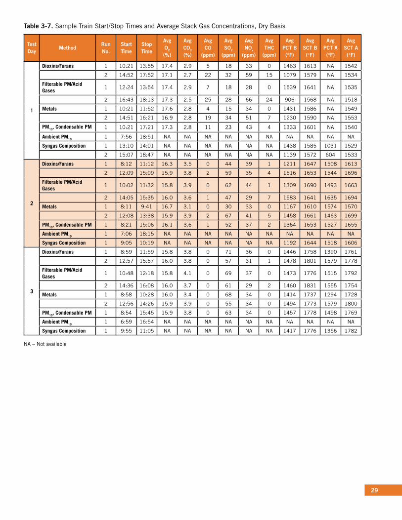
29

Table 3-7. Sample Train Start/Stop Times and Average Stack Gas Concentrations, Dry Basis

Test Day

MethodRun No.

Start Time

Stop Time

Avg O2 (%)

Avg CO2 (%)

Avg CO

(ppm)

Avg SO2

(ppm)

Avg NOx

(ppm)

Avg THC

(ppm)

Avg PCT B (°F)

Avg SCT B (°F)

Avg PCT A (°F)

Avg SCT A (°F)

1

Dioxins/Furans 1 10:21 13:55 17.4 2.9 5 18 33 0 1463 1613 NA 1542

2 14:52 17:52 17.1 2.7 22 32 59 15 1079 1579 NA 1534

Filterable PM/Acid Gases

1 12:24 13:54 17.4 2.9 7 18 28 0 1539 1641 NA 1535

2 16:43 18:13 17.3 2.5 25 28 66 24 906 1568 NA 1518

Metals 1 10:21 11:52 17.6 2.8 4 15 34 0 1431 1586 NA 1549

2 14:51 16:21 16.9 2.8 19 34 51 7 1230 1590 NA 1553

PM10, Condensable PM 1 10:21 17:21 17.3 2.8 11 23 43 4 1333 1601 NA 1540

Ambient PM10 1 7:56 18:51 NA NA NA NA NA NA NA NA NA NA

Syngas Composition 1 13:10 14:01 NA NA NA NA NA NA 1438 1585 1031 1529

2 15:07 18:47 NA NA NA NA NA NA 1139 1572 604 1533

2

Dioxins/Furans 1 8:12 11:12 16.3 3.5 0 44 39 1 1211 1647 1508 1613

2 12:09 15:09 15.9 3.8 2 59 35 4 1516 1653 1544 1696


1 10:02 11:32 15.8 3.9 0 62 44 1 1309 1690 1493 1663

2 14:05 15:35 16.0 3.6 1 47 29 7 1583 1641 1635 1694

Metals 1 8:11 9:41 16.7 3.1 0 30 33 0 1167 1610 1574 1570

2 12:08 13:38 15.9 3.9 2 67 41 5 1458 1661 1463 1699

PM10, Condensable PM 1 8:21 15:06 16.1 3.6 1 52 37 2 1364 1653 1527 1655



3

Dioxins/Furans 1 8:59 11:59 15.8 3.8 0 71 36 0 1446 1758 1390 1761

2 12:57 15:57 16.0 3.8 0 57 31 1 1478 1801 1579 1778


1 10:48 12:18 15.8 4.1 0 69 37 0 1473 1776 1515 1792

2 14:36 16:08 16.0 3.7 0 61 29 2 1460 1831 1555 1754

Metals 1 8:58 10:28 16.0 3.4 0 68 34 0 1414 1737 1294 1728

2 12:56 14:26 15.9 3.9 0 55 34 0 1494 1773 1579 1800

PM10, Condensable PM 1 8:54 15:45 15.9 3.8 0 63 34 0 1457 1778 1498 1769



NA – Not available

30

Table 3-8. CEM Average Measurements, Dry Basis

Test Day TimeStack O2

(%)Stack CO2

(%)Stack CO

(ppm)Stack NOx

(ppm)Stack SO2

(ppm)Stack THC

(ppm)SC O2 (%)

SC CO2 (%)

1 10:21-13:55 17.4 2.6 0 34 12 0 13.2 6.4

1 14:52-17:52 16.7 3.1 19 39 42 6 11.9 7.3

2 8:12-11:12 17.0 3.0 0 34 30 0 10.8 7.9

2 12:09-15:09 16.2 3.7 0 41 70 4 9.8 8.6

3 8:59-11:59 16.4 4.0 0 41 75 0 6.5 10.8

3 12:57-15:57 16.5 3.9 NA* 42 62 0 7.3 10.6

NA - Not Available - CO monitor operating at secondary combustion zone

Table 3-9. Stack Velocities and Flow Rates

Run Number Gas Velocity Volumetric Flowrate Volumetric Flowrate

ft/sec acfm scfm

I-M5/26A-1 13.6 5141 2280

I-M5/26A-2 14 .9 5636 2516

II-M5/26A-1 14.5 5501 2279

II-M5/26A-2 14.8 5583 2338

III-M5/26A-1 13.9 5277 2334

III-M5/26A-2 14.4 5439 2330

I-M29-1 13.4 5067 2233

I-M29-2 14.2 5380 2311

II-M29-1 14.7 5561 2323

II-M29-2 16.1 6082 2598

III-M29-1 14.3 5396 2551

III-M29-2 14.4 5459 2433

I-M23-1 14.6 5540 2379

I-M23-2 14.9 5628 2446

II-M23-1 15.0 5684 2504

II-M23-2 13.9 5252 2264

III-M23-1 14.3 5410 2410

III-M23-2 14.6 5535 2338

Average 14.5 5476 2382

31

The pollutant concentrations were converted into mass emission rates using the following equation:

Mass Emissions =CiMiQs

106RT(13)

where Ci is the concentration of pollutant i in ppm, Mi is the molecular mass of pollutant i, Qs is the stack flow rate in standard cubic feet per hour, R is the ideal gas constant, and T is the temperature (for standard conditions, 68 °F [20 ºC]).

3.4 Particulate Matter

3.4.1 Ambient ParticulateTable 3-10 lists the results from the ambient sampler. These data reflect the amount of PM10 that was being pulled into the dilution air of the stack. The results from March 3 and March 4 are similar, with the Test Day 3 (March 5, 2008) results significantly lower, possibly due to a heavy rain the night before. Overall, the ambient particulate loading represented no more than 1 mg/m3 on any given day.

3.4.2 Total Filterable ParticulateTable 3-11 lists the results for the total filterable particulate for Test Day 1 through Test Day 3. Based on the ambient PM10 measurements, approximately 5% of this particulate resulted from material being pulled into the dilution air from

the ambient surroundings. These results show an average of 26 mg/Nm3 with a standard deviation of 9 mg/Nm3. The average emission rate was 0.224 lb/hr over the three test days of burning animal carcasses, with a standard deviation of 0.077 lb/hr.

3.4.3 Filterable Particulate Matter and Condensable Particulate MatterTable 3-12 shows the results from the filterable particulate (EPA Method 5) and condensable particulate (EPA Method 202). Total particulate averaged 21.9 mg/Nm3 (not corrected for dilution). No particulate matter with an aerodynamic diameter greater than 10 µm was observed. Note that the total filterable particulate results are slightly different in Table 3-12 than in Table 3-11, because the sample train in Table 3-12 was run for 420 minutes as opposed to 90 minutes for the results shown in Table 3-11. Approximately 1/3 of the total particulate was condensable, and of that fraction, approximately 15% was organic, so approximately 30% of the particulate was composed of condensable sulfates and nitrates. Note that the contribution of ambient particulate (approximately 1 mg/Nm3) was not subtracted from the total filterable particulate, although based on the dilution ratios (which averaged 2.34 over Test Days 1 through 3) and results from the ambient sampling, ambient particulate would be expected to contribute roughly 1.34 mg/Nm3 or approximately 5% of the total filterable particulate.

Table 3-10. Ambient PM10 Results

Test Day Run Duration (min) Sample Volume (m3) Filter Catch (µg) PM10 (µg/m3)

1 674.4 864.94 849,900 982.6

2 564.6 725.34 710,600 979.7

3 590.4 761.32 38,290 50.3

Table 3-11. Total Filterable Particulate Results

Test Day Run Concentration (mg/Nm3) Emission Rate (lb/hr)

1 1 15.1 0.129

1 2 13.7 0.129

2 1 34.6 0.295

2 2 33.5 0.294

3 1 27.5 0.240

3 2 29.3 0.256

32

3.4.4 Visible EmissionsOpacity measurements were taken with EPA Method 9 on Day 4, and on Days 1 through 3, intermittent opacity measurements were taken (approximately 15 minutes per hour of sampling), although the sample frequency and duration criteria for EPA Method 9 were not satisfied on those days due to personnel limitations. On Days 1 through 3,

no measurable opacity was observed during any of the time periods where visible emissions observations were taken. On Day 4, during the vegetable matter burns, EPA Method 9 measurements were taken according to the method. These measurements are listed in Table 3-13. The peak smoke number observed during the vegetative matter burns was 15%, with the peak opacity over the test day at 9.4%.

Table 3-12. Particulate Matter Emissions Measurements

Day 1 Day 2 Day 3 Average

FILTERABLE PARTICULATE < 10µm

Concentration, gr/DSCF 2.04E-03 7.29E-03 8.27E-03 5.87E-03

Concentration, mg/DSCM 4.68 16.69 18.92 13.43

Emission Rate, lb/hr 0.1045 0.3645 0.4226 0.2972

ORGANIC CONDENSABLE PARTICULATE




INORGANIC CONDENSABLE PARTICULATE




TOTAL PARTICULATE < 10µm




TOTAL FILTERABLE PARTICULATE




TOTAL PARTICULATE




Table 3-13. Visible Emissions During Vegetable Matter Tests (Day 4)

Start Time End Time Opacity (%)

11:14 12:14 0

13:33 14:42 9.4

33

3.4.5 Particle Size DistributionsTable 3-14 shows the particle size distributions for Test Days 1 through 3. The particulate matter was very fine, with an average of 58.1% by mass ending up on the backup filter. Virtually all the particulate had an aerodynamic diameter less than 0.5 µm. Figure 3-29 shows the cumulative mass percent versus particle size for the average of the three runs.

3.5 Hydrogen Chloride and ChlorineTable 3-15 lists the hydrogen chloride (HCl) and chlorine (Cl2) emissions. HCl averaged 30.8 mg/Nm3 with a standard deviation of 19.2 mg/Nm3, and Cl2 averaged 0.173 mg/

Nm3 with a standard deviation of 0.486 mg/Nm3. The average emission rate of HCl was 0.27 lb/hr with a standard deviation of 0.17 lb/hr and the average emission rate of Cl2 was 0.0015 lb/hr with a standard deviation of 0.0014 lb/hr. These particular pollutants showed a relatively high degree of variability, with the higher emissions occurring at the higher animal carcass feed rates. This variability may result from differences in the feed that the gasified animals were fed.

Table 3-14. Particle Size Distribution Data (Mass Basis)

Day 1 Day 2 Day 3 Average

StageAerodynamic Particle Size

(µm)

Mass % of Total

Cum. Mass % Less Than

Mass % of Total


Mass % of Total


Mass % of Total


1 8.79 0.4 99.6 0.0 100.0 0.0 100.0 0.1 99.9

2 5.47 0.0 99.6 0.0 100.0 0.0 100.0 0.0 99.9

3 3.71 0.0 99.6 0.0 100.0 0.0 100.0 0.0 99.9

4 2.54 0.0 99.6 0.0 100.0 0.0 100.0 0.0 99.9

5 1.62 0.0 99.6 0.8 99.2 0.7 99.3 0.5 99.4

6 0.77 0.7 98.9 4.8 94.5 0.8 98.6 2.1 97.3

7 0.49 11.9 87.0 11.8 82.6 3.8 94.7 9.2 88.1

8 0.33 32.2 54.8 38.7 43.9 19.2 75.5 30.1 58.1

Backup < 0.33 54.8 0.0 43.9 0.0 75.5 0.0 58.1 0.0

Total 100.0 100.0 100.0 100.0

0

20

40

60

80

100

120

0 2 4 6 8 10

Dp - Aerodynamic Particle Diamter (µm)

Cum

ulat

ive

Mas

s %

Les

s th

an

Figure 3-29. Particle Size Distribution

34

Table 3-15. Hydrogen Chloride and Chlorine

Test Day RunHCl

(mg/Nm3)HCl Emission Rate

(lb/hr)Chlorine as Cl2

(mg/Nm3)Chlorine Emission

Rate (lb/hr)

1 1 13.8 0.118 0.066 0.000561 2 4.1 0.039 0.092 0.000862 1 32.0 0.273 0.469 0.004002 2 57.8 0.507 0.127 0.001123 1 37.1 0.324 0.112 0.000983 2 39.8 0.348 ND ND

ND - Not Detected

3.6 MetalsMetals concentrations were low, being comparable to or lower than the New Source Performance Standards (NSPS) for metals for small municipal waste combustors [Federal Register, 2000]. Table 3-16 lists the concentrations and emission rates of metals at the stack. Antimony, beryllium,

cobalt, and mercury were not detected. The source of cadmium is not known – animal carcasses are not expected to have much Cd, and the fuel oil had none. Cd may be a component in the materials of construction of the gasifier or the macerator.

35

Table 3-16. Metals Results

Day1 Run 1

Day 1 Run 2

Day 2 Run 1

Day 2 Run 2

Day 3 Run 1

Day 3 Run 2

Average

Antimony

Concentration, µg/Nm3 ND ND ND ND ND ND ND

Emission Rate, lb/hr ND ND ND ND ND ND ND

Arsenic

Concentration, µg/Nm3 0.49 0.84 0.77 1.41 1.31 1.99 1.13

Emission Rate, lb/hr 4.07E-06 7.28E-06 6.67E-06 1.38E-05 1.25E-05 1.81E-05 1.04E-05

Barium

Concentration, µg/Nm3 5.02 2.98 5.14 4.38 10.80 ND 5.66

Emission Rate, lb/hr 4.20E-05 2.58E-05 4.47E-05 4.26E-05 1.03E-04 ND 5.16E-05

Beryllium


Emission Rate, lb/hrND ND ND ND ND ND ND

Cadmium



Chromium



Cobalt



Lead



Manganese



Mercury



Nickel



Selenium



Silver



ND - Not Detected

36

3.7 PCDDs/FsThe measured dioxins and furans were very low, with concentrations in the picogram per normal cubic meter range (pg/Nm3). As a reference, the NSPS for dioxins from small municipal waste combustors [Federal Register, 2000] is 13 ng/Nm3 total PCDD/F, which is approximately an order of magnitude higher than the observed gasifier emissions, when corrected to 12 % CO2. Table 3-17 lists the concentrations of

PCDDs/Fs as well as the concentration in Toxic Equivalency (TEQ) units, which represent a weighted concentration based on World Health Organization (WHO) 2005 toxicity equivalency factor (TEF) weights (Van den Berg et al., 2006). Table 3-18 lists the mass emission rates of PCDDs/Fs in lb/hr, including TEQ units. Note that averaging is based on setting non-detects to zero.

Table 3-17. PCDD/F Concentrations (pg/Nm3)

Day 1 Run 1

Day 1 Run 2

Day 2 Run 1

Day 2 Run 2

Day 3 Run 1

Day 3 Run 2

Average

2,3,7,8-TCDD ND ND ND ND ND ND ND

1,2,3,7,8-PeCDD ND ND ND ND ND ND ND

1,2,3,4,7,8-HxCDD ND ND ND ND ND ND ND



1,2,3,4,6,7,8-HpCDD 2.6 ND ND ND 2.5 ND 0.8

OCDD 6.2 7.0 ND 8.0 4.5 5.9 5.3

2,3,7,8-TCDF 5.7 5.7 1.2 1.3 0.8 ND 2.4

1,2,3,7,8-PeCDF 3.7 4.2 ND ND ND ND 1.3

2,3,4,7,8-PeCDF 7.8 15.4 ND ND ND ND 3.9

1,2,3,4,7,8-HxCDF 3.6 7.7 ND ND ND ND 1.9

1,2,3,6,7,8-HxCDF 2.4 3.7 ND ND ND ND 1.0

2,3,4,6,7,8-HxCDF 3.5 6.1 ND ND ND ND 1.6

1,2,3,7,8,9-HxCDF ND ND ND ND ND ND ND

1,2,3,4,6,7,8-HpCDF 4.5 6.3 ND ND 2.5 3.3 2.8

1,2,3,4,7,8,9-HpCDF ND ND ND ND ND ND ND

OCDF 5.8 ND ND ND ND ND 1.0

TEQ 4.1 7.1 0.1 0.1 0.1 0.0 1.9

Other TCDD 16.5 21.3 59.5 104.0 89.0 79.8 61.7

Other PeCDD ND 4.7 11.4 10.2 10.8 13.3 8.4

Other HxCDD ND ND ND ND 4.1 5.0 1.5

Other HpCDD 2.2 5.1 ND ND 3.4 ND 1.8

Total PCDD 27.5 38.1 70.9 122.2 114.2 104.0 79.5

Other TCDF 125.0 44.4 62.4 79.6 70.6 88.2 78.4

Other PeCDF 46.2 65.0 15.8 15.1 13.2 18.1 28.9

Other HxCDF 14.9 27.2 4.0 7.3 6.6 9.5 11.6

Other HpCDF 9.4 6.3 1.4 1.4 2.5 3.3 4.1

Total PCDF 232.6 192.0 84.8 104.7 96.2 122.3 138.8

ND – Not Detected

37

Table 3-18. PCDD/F Mass Emission Rate (lb/hr)

Day 1 Run 1

Day 1 Run 2

Day 2 Run 1

Day 2 Run 2

Day 3 Run 1

Day 3 Run 2

Average

2,3,7,8-TCDD ND ND ND ND ND ND ND

1,2,3,7,8-PeCDD ND ND ND ND ND ND ND




1,2,3,4,6,7,8-HpCDD 2.26E-11 ND ND ND 2.22E-11 ND 7.47E-12

OCDD 5.51E-11 6.38E-11 ND 6.75E-11 4.02E-11 5.19E-11 4.64E-11

2,3,7,8-TCDF 5.09E-11 5.18E-11 1.16E-11 1.07E-11 7.08E-12 ND 2.20E-11

1,2,3,7,8-PeCDF 3.26E-11 3.85E-11 ND ND ND ND 1.19E-11

2,3,4,7,8-PeCDF 6.96E-11 1.40E-10 ND ND ND ND 3.49E-11

1,2,3,4,7,8-HxCDF 3.21E-11 7.05E-11 ND ND ND ND 1.71E-11



1,2,3,7,8,9-HxCDF ND ND ND ND ND ND ND

1,2,3,4,6,7,8-HpCDF 3.97E-11 5.70E-11 ND ND 2.28E-11 2.88E-11 2.47E-11

1,2,3,4,7,8,9-HpCDF ND ND ND ND ND ND ND

OCDF 5.15E-11 ND ND ND ND ND 8.58E-12

TEQ 3.60E-11 6.49E-11 1.16E-12 1.09E-12 1.17E-12 3.04E-13 1.75E-11

Other TCDD 1.46E-10 1.94E-10 5.58E-10 8.80E-10 8.04E-10 6.99E-10 5.47E-10

Other PeCDD ND 4.24E-11 1.07E-10 8.63E-11 9.73E-11 1.17E-10 7.50E-11

Other HxCDD ND ND ND ND 3.72E-11 4.36E-11 1.35E-11

Other HpCDD 1.94E-11 4.66E-11 ND ND 3.02E-11 ND 1.60E-11

Total PCDD 2.43E-10 3.47E-10 6.65E-10 1.03E-09 1.03E-09 9.12E-10 7.05E-10

Other TCDF 1.11E-09 4.05E-10 5.85E-10 6.75E-10 6.38E-10 7.72E-10 6.98E-10

Other PeCDF 4.10E-10 5.92E-10 1.48E-10 1.28E-10 1.19E-10 1.58E-10 2.59E-10

Other HxCDF 1.33E-10 2.48E-10 3.72E-11 6.20E-11 5.91E-11 8.29E-11 1.04E-10

Other HpCDF 8.37E-11 5.70E-11 1.35E-11 1.21E-11 2.28E-11 2.88E-11 3.63E-11

Total PCDF 2.07E-09 1.75E-09 7.95E-10 8.88E-10 8.69E-10 1.07E-09 1.24E-09

ND – Not Detected

38

3.8 Synthesis Gas CompositionThe analyses of the synthesis gas were inconclusive because the analytical results did not indicate a gas that resembled a typical gasifier synthesis gas. The composition of the gas indicated that nearly complete combustion had occurred by the time the gases were sampled. Nearly complete combustion could have occurred due to infiltration of ambient air into the PCs via leaks between the SC and PC, or perhaps an overabundance of ambient air was allowed to enter the primary chambers through the ports in the doors, or a recirculation zone from the burner region could have resulted in air being mixed into the back end of the PC through turbulent mixing. At any rate, the high oxygen concentration

in some of the samples indicated that significant quantities of ambient air were being pulled into the chambers. It was not possible to determine which situation had occurred, although it is possible that the truncated shakedown schedule resulted in sub-optimal stoichiometric ratios in the primary chambers. Table 3-19 lists the results from the analysis of the synthesis gas samples.

3.9 Ash AnalysisThe ash samples that were subjected to TCLP analysis (Table 3-20) mostly showed non-detects for all target metals. The amino acid analytical results for the ash (Table 3-21) showed all amino acids below reportable detection limits.

Table 3-19. Synthesis Gas Composition

H2 (%) CO2 (%) O2 (%) N2 (%) CO (%)Methane (ppm)

Non-Methane Organic

Compounds (ppm)

H2O (mg/L)

Day 1 Run 1 ND 6.9 14.7 84.8 ND 20 436 221

Day 1 Run 2 ND 9.5 7.9 76.6 ND 1923 2507 334

Day 2 Run 1 ND 9.1 12.7 86.2 ND 1503 1063 11424

Day 3 Run 1 ND ND 23.2 83.7 ND 453 1351 100

Table 3-20. TCLP Results for Ash (mg/L)

As Ba Cd Cr Pb Hg Se Ag

Day 2 Side A <0.015 0.05 < 0.0006 < 0.05 <0.015 < 0.001 < 0.03 < 0.06

Day 2 Side B <0.015 0.04 < 0.0006 < 0.05 <0.015 < 0.001 < 0.03 < 0.06

Day 3 Side A <0.015 < 0.03 < 0.0006 0.08 <0.015 < 0.001 < 0.03 < 0.06

Day 3 Side B <0.015 0.05 < 0.0006 < 0.05 <0.015 < 0.001 < 0.03 < 0.06

Day 4 Side A <0.015 <0.03 < 0.0006 < 0.05 <0.015 < 0.001 < 0.03 < 0.06

Day 4 Side B <0.015 0.06 < 0.0006 < 0.05 <0.015 < 0.001 < 0.03 < 0.06

39

Table 3-21. Amino Acid Analytical Results for Ash (mg/g)

Day 2 Side A

Day 2 Side B

Day 3 Side A

Day 3 Side B

Day 4 Side A

Day 4 Side B

Alanine < 0.5 < 0.5 < 0.5 < 0.5 < 0.5 < 0.5

Arginine < 0.5 < 0.5 < 0.5 < 0.5 < 0.5 < 0.5

Aspartic Acid < 0.5 < 0.5 < 0.5 < 0.5 < 0.5 < 0.5

Glutamic Acid < 0.5 < 0.5 < 0.5 < 0.5 < 0.5 < 0.5

Glycine < 0.5 < 0.5 < 0.5 < 0.5 < 0.5 < 0.5

Histidine < 0.5 < 0.5 < 0.5 < 0.5 < 0.5 < 0.5

Isoleucine < 0.5 < 0.5 < 0.5 < 0.5 < 0.5 < 0.5

Leucine < 0.5 < 0.5 < 0.5 < 0.5 < 0.5 < 0.5

Lysine < 0.5 < 0.5 < 0.5 < 0.5 < 0.5 < 0.5

Methionine < 0.5 < 0.5 < 0.5 < 0.5 < 0.5 < 0.5

Phenylalanine < 0.5 < 0.5 < 0.5 < 0.5 < 0.5 < 0.5

Proline < 0.5 < 0.5 < 0.5 < 0.5 < 0.5 < 0.5

Serine < 0.5 < 0.5 < 0.5 < 0.5 < 0.5 < 0.5

Threonine < 0.5 < 0.5 < 0.5 < 0.5 < 0.5 < 0.5

Tryptophan < 0.5 < 0.5 < 0.5 < 0.5 < 0.5 < 0.5

Tyrosine < 0.5 < 0.5 < 0.5 < 0.5 < 0.5 < 0.5

Valine < 0.5 < 0.5 < 0.5 < 0.5 < 0.5 < 0.5

3.10 Estimated Emissions of Pollutants Per Mass of Carcass FedTaking the average emissions of each pollutant in pounds per hour and dividing by the average carcass feed rate (0.32 tons/hr) yields the estimated emissions in emission factor

units. These results are shown in Table 3-22. Note that these results apply only to the animal carcass feed, since extractive sampling was not performed during the plant matter tests for reasons described earlier.

40

Table 3-22. Estimated Emissions

Average lb/hr Average lb/ton of carcass

Total Filterable Particulate 0.297 0.93

PM10 0.297 0.93

Organic Condensable Particulate 0.022 0.07

Inorganic Condensable Particulate 0.120 0.37

Total Particulate 0.439 1.37

Hydrogen Chloride 0.27 0.84

Chlorine as Cl2 0.173 0.54

Antimony ND ND

Arsenic 1.04E-05 3.25E-05

Barium 5.16E-05 1.61E-04

Beryllium ND ND

Cadmium 1.08E-04 3.38E-04

Chromium 6.11E-05 1.91E-04

Cobalt ND ND

Lead 5.50E-05 1.72E-04

Manganese 4.69E-05 1.47E-04

Mercury ND ND

Nickel 1.00E-04 3.13E-04

Selenium 4.11E-05 1.28E-04

Silver 7.23E-06 2.26E-05

PCDD/F Total 1.24E-09 3.88E-09

PCDD/F TEQ 1.75E-11 5.47E-11

ND = Not detected.

41

4.0 Quality Assurance/Quality Control

Evaluation Report

This project was conducted under an approved Category III QAPP titled Source Sampling for Transportable Gasifier for Animal Carcasses and Contaminated Plant Material (November 2007). Measurement Quality Objectives (MQOs) established in the QAPP in terms of accuracy, precision, and completeness are shown in Table 4-1 of the QAPP.

Flow rates of stack gas and dilution air were determined using EPA Methods 1 and 2. MQOs were evaluated by pre- and post-test leak checks. All leak checks performed during the course of sampling passed method criteria. Moisture content of the stack gas was determined using EPA Method 4. MQOs were evaluated by pre- and post-test leak checks. All leak checks that were performed passed method criteria. These measurements were 100% complete.

4.1 CEMs (CO2/O2, SO2, NOx, CO, THCs) CEMs were calibrated prior to each test day at three points and pre-test and post-test bias checks were performed. Direct calibration MQOs were established at ±2% error. All values measured for O2, CO, SO2 and NOx were within the MQOs. For CO2, one measured value was slightly outside the MQO at 2.3%. THC values were routinely outside the ±2% limit, ranging from 0 to 6.2%. The bias check MQO was established at ±5% for all CEMs and was routinely met for all instruments with the exception of the THC analyzer, which ranged from 0 to 13.9% error. The MQO for zero/drift checks was established at ±3% and measured on the CO2, O2, SO2, and CO CEMs daily. The MQOs were met for all measurements with the exception of one CO2 and one SO2 measurement, which were slightly above the MQO at ±4.2%. In conclusion, CEM measurements met 90% completeness with the exception of THC.

4.2 HCl, Cl2 (Method 26/26A)Samples were analyzed for HCl and Cl2 using EPA Method 26A by Resolution Analytics. Results from QC samples were included with the analytical report. Reagent blanks and field blanks for HCl were all below method detection limits. For Cl2, the reported catch on the field blank was 0.048 mg. Because Cl2 sample results were low, this blank value is significant. A matrix spike was performed by the addition of a known amount of chloride standard. Recoveries ranged from 90 to 103%, which met acceptance criteria for accuracy. Precision was assessed by replicate injection of laboratory control samples and the replicate injections resulted in a 1.5% difference, which meets established MQOs. These analyses were 100% complete.

4.3 Filterable Particulate (Method 5) Tare weights for filters were obtained by ARCADIS on 02/29/08 and analyzed by Resolution Analytics. Final weights were obtained on 04/30/08. For each weighing session the balance was zeroed and a 5.0000 mg calibration weight was weighed before and after the sample filters. One sample filter (Filter No. 5830786) was also processed as a blank. Accuracy was assessed by comparing the observed weight of the 5.0000 mg calibration standard to the known value. Precision was assessed using the values from replicate weighings of the 5.0000 mg standard. MQOs were met and these measurements were 100% complete.

4.4 PCDDs/PCDFs (EPA Method 23)Six samples, a field blank and reagent blanks were submitted to Analytical Perspectives for the determination of PCDD/PCDF. The laboratory report included raw data for initial calibration, calibration verifications, and daily laboratory control samples. No analytes were detected in the field blank, reagent blanks, or method blank. Internal standard and surrogate recoveries were within the acceptable range of 50–150% for all samples and met MQOs for accuracy/bias. No criteria for precision were established but standard deviations between replicate injections of laboratory control samples passed method acceptance criteria. These analyses were 100% complete.

4.5 Metals (EPA Method 29)EPA Method 29 trains were sent to First Analytical Laboratories for analysis of target metals antimony, arsenic, barium, beryllium, cadmium, chromium, cobalt, lead, manganese, mercury, nickel, selenium, and silver. Barium, cobalt, and manganese were determined by Inductively Coupled Plasma Optical Emission Spectrometry (ICP). Mercury was determined by Cold Vapor Atomic Absorption Spectrophotometry (CVAA). All other compounds were determined by Graphite Furnace Atomic Absorption Spectrophotometry (GFAA).

Six sampled trains were submitted for analysis along with a field blank and reagent blanks. Normal trace amounts of barium, cadmium, chromium, and manganese were found in the blank trains. Since sample values were so low for these elements, blank concentrations are significant and samples should be blank-corrected.

Laboratory control samples consisting of initial calibration verifications (ICVs), continuing calibration verifications (CCVs) and continuing calibration blanks (CCBs) were

42

performed for each element. Triplicate values are obtained for each sample on the instrument and the average of these triplicate values is reported. In addition, the laboratory performed duplicate analysis and matrix spike analysis for selected samples. All laboratory control samples were within the acceptance criteria for recovery and relative standard deviation required by the method.

4.6 PM10, Condensable Particulate (EPA M201A/OTM-DIM)These samples were analyzed by Resolution Analytics. Leak checks on the sampling trains were performed according to the method for every test. Tests were not started until leak checks passed.

4.7 CO2, CH4, N2, O2, NMOC, CH4 in Synthesis GasLeak checks on the sampling trains were performed according to the method for every test. Tests were not started until leak checks passed.

4.8 Total Suspended ParticulateThese samples were analyzed by Resolution Analytics. Leak checks on the sampling trains were performed according to the method for every test. Tests were not started until leak checks passed.

4.9 Ash Composition (EPA Method 1311/TCLP)Grab samples of the ash were taken from “A”-side and “B”-side on days 2 through 4. Six samples were submitted to First Analytical Laboratories for TCLP analysis for target elements arsenic, barium, cadmium, chromium, lead, mercury, selenium, and silver. Arsenic, cadmium, lead, mercury, selenium, and silver were not detectable in any of the leachates. The arsenic spike recovery was slightly low at 70%. This low recovery was not considered a problem because there were not quantifiable levels of arsenic in the samples. All of the other spike recoveries were within the acceptable range of 75–125%. All leachates were analyzed in duplicate. Results for laboratory control samples including method blanks, initial calibration verifications, continuing calibration verifications, and continuing calibration blanks were also included in the analytical report. All data were within method acceptance criteria. These analyses were 100% complete.

4.10 Ash Amino AcidsGrab samples of the ash were taken from “A”-side and “B”-side on days 2 through 4. A total of six samples were submitted to EMSL Analytical for a complete amino acid profile, which included the following:

• Acid stable amino acids;

• Sulfur amino acids; and

• Tryptophan.

For amino acids, a portion of sample was mixed with hydrochloric acid solution in a modified Kjeldahl flask. To prevent oxidation, as much oxygen as possible is removed from the flask by repeated freezing and thawing under vacuum. The neck of the flask was heat-sealed and the flask was heated in a 110 °C oven for 20 hours. Proteins in the sample were hydrolyzed to amino acids by the hot hydrochloric acid solution. Amino acids (if present) were separated on an ion exchange column and detected by reaction with ninhydrin. The concentration of each amino acid was quantitated against a standard known concentration.

The tryptophan samples were hydrolyzed with sodium hydroxide in an evacuated sealed glass vessel. Hydrolysates were analyzed on a high performance liquid chromatograph (HPLC), using UV detection and quantitated from standards of known concentration.

Results for all samples were below the laboratory reporting limit of 0.5 mg/g.

4.11 Data Quality Assessment (DQA)An internal DQA was performed to ensure data from raw analytical reports were accurately transcribed and entered into spreadsheets. Results of laboratory quality control samples for all methods were also reviewed. An error in data entry for organic and inorganic condensable particulate was found and corrected. All laboratory control samples for all methods met method acceptance criteria.

43

5.0 Conclusions

A prototype transportable gasifier, developed by BGP for the Department of Defense TSWG, was tested in the field in March 2008. The gasifier is intended to thermally process contaminated animal carcasses and plant matter.

Samples were taken and analyzed for several targets, including:



• Metals;

• Acid gases;

• Polychlorinated dibenzo-p-dioxins and polychlorinated dibenzofurans;



The unit was deployed in the field in a rapid manner, and was operational to perform the necessary emissions testing described in the QAPP in spite of having less than a week for initial startup and shakedown. This truncated shakedown schedule resulted in several operational issues that should be addressed through minor design modifications, discussed in the Engineer’s Report [BGP, 2008]. The operational issues of concern that impacted the emissions testing included:

• Failure of the ash removal auger contributed to a feed rate limitation.

• Inefficient distribution of animal matter on the hearths in the primary chamber limited the unit’s maximum throughput to approximately 32% of the design capacity.

• The plant material selected as a surrogate for contaminated plant matter was not acceptable to feed through the unit’s macerator. Gasifier operation with plant matter feed was therefore cut to only a few hours and extractive sampling was not performed on the plant matter tests.

• Air infiltrated into the primary chambers through some unknown mechanism, and the analyzed synthesis gas did not bear a resemblance to synthesis gas from other gasification processes, possibly due to air migrating from the secondary chambers through gaps in the hearth to the primary chamber in the vicinity of the sampling port, turbulent mixing from the burner zones, or an overabundance of air being pulled in through the ports in the doors.

• Emissions of the measured pollutants were at low levels, and the ash passed TCLP. There were slightly elevated emissions of cadmium, the source of which is unknown. There may be Cd present in the materials of construction of the gasifier or macerator, since animal carcasses are not known to contain large amounts of Cd and the fuel oil did not contain any Cd.

There are no emissions standards with which to compare this type of gasifier unit, although emissions of most pollutants were well below the NSPS for small municipal waste combustors. The particle size distribution suggested that the vast majority of the emitted particulate matter was smaller than 0.5 microns.

A very important observation was that the emissions of carbon monoxide and total hydrocarbons correlated very well with the average of the temperatures of the two primary chambers. This observation suggests that for emergency response deployment, the primary chamber temperatures could be used as a surrogate monitoring parameter to ensure minimization of emissions. Additional testing should investigate this potential advantage.

Amino acid analysis of the ash yielded non-detects for all target analytes. This observation suggests that the gasifier unit would be capable of destroying prions that could potentially cause Transmissible Spongiform Encephalopathy (TSE).

Because the unit is so simple and produces such low emissions, it is important to gain a better understanding of the reactions taking place in the primary chambers. It is also unknown whether the low emissions will persist as the unit is brought up to its full operating capacity, although by normalizing the results versus the feed rate into emission factor units, the estimated emissions should be conservative. In addition, operation at full capacity may result in significant reduction in auxiliary fuel usage. Further testing at full capacity would be very desirable.

According to the introduction, the purposes of this emissions test were:





44

The data presented in this report are of sufficient quality to allow these goals to be achieved.

The overall program objective was to deliver a prototype gasifier capable of being transported over all primary and secondary roads, for this prototype gasifier to be capable of being operational in less than 24 hours after arrival at the

site, and for this prototype gasifier to have the capability to process 25 tons per day of contaminated animal carcasses or plants.

The first two program objectives were achieved; the third objective has yet to be demonstrated.

45

6.0 References

ARCADIS, 2007, Quality Assurance Project Plan, “Source Sampling for Transportable Gasifier for Animal Carcasses and Contaminated Plant Material,” December 12, 2007.

BGP, 2008, Engineering Report: Initial Shakedown and Testing of Mobile Gasifier Prototype; DoD Contract Number: W91CRB-06-C-0007.

EPA, 1995, AP-42 Emission Factor Database, http://www.epa.gov/ttn/chief/ap42/index.html

Federal Register, 2000, 40 CFR Part 60. New Source Performance Standards for New Small Municipal Waste Combustion Units; Final Rule Wednesday, December 6, 2000.

Van den Berg, M., et al., 2006. “The 2005 World Health Organization Reevaluation of Human and Mammalian Toxic Equivalency Factors for Dioxins and Dioxin-Like Compounds,” Toxicological Sciences 2006 93(2):223–241.

http://www.epa.gov/ttn/chief/ap42/index.html

United StatesEnvironmental ProtectionAgency

Office of Research and DevelopmentNational Homeland Security Research CenterCincinnati, OH 45268Official BusinessPenalty for Private Use$300

PRESORTED STANDARDPOSTAGE & FEES PAID

EPAPERMIT NO. G-35

SCIENCE

FINAL REPORT CE

Documents

Transcript of FINAL REPORT CE