Final Exam - CSSERVERreising/ME 224/Binder1.pdfROSE-HULMAN INSTITUTE OF TECHNOLOGY Department of...
21
Final Exam: MATLAB Arrays, operations (arithmetic, relational) programming structures: for/while loops, if...elseif...else...end standard mathematical functions in MATLAB, scientific notation creating MATLAB functions, for example functions that sum a series, functions that create/process arrays, functions that calculate (polynomials, interpolants, iterations, etc) simulating cellular automata (nothing specific on Wolfram’s coding system) graphics: 2-D plots, of functions and parametric curves, images of arrays via imagesc/image, colormaps images of function data via pcolor. 3-D plots via surf, domains in polar coordinates preparing arrays for plotting using meshgrid, plotting in other coordinate systems. Plotting curves in space. Math Iteration x n1 fx n , fixed points and convergence/divergence, stability/instability linear convergence and the derivative f x , checking for linear convergence experimentally Newton’s method for finding roots of functions, quadratic convergence Iteration/recurrence relations in general - developing a sequence of numbers, arrays, etc according to a rule Interpolation: Formulating equations, calculating the interpolant, plotting the interpolant, the data, and the error (if applicable). Standard polynomial interpolation, interpolation with special families (e.g. odd powers only, sines and cosines, etc) Least squares: The least-squares solution of a linear system Least squares fit of (x,y) data Least square approximation of a function by sampling data Plotting the least squares data fit along with the data, plotting the error (relative to the datapoints or to the underlying function if there is one) How to simulate a discrete probability distribution 1 with prob p, 0 with prob 1-p : u(randp) or u(rand(1,N)p) A random matrix of 1’s and 0’s with probability p of 1 A distribution: 1 with prob p 1 , 2 with prob p 2 , ..., n with prob p n Displaying the results of a simulation using Nhist(Y,X) where X specified "bin centers" Simulating a random walk with steps of 1/-1 or random size in [-1,1], 2*(rand.5)-1 or 2*rand-1 respectively; keeping track of stuff (what was the max or min, where did you wind up, how many times did you hit zero, etc) 1
-
Upload
hoanghuong -
Category
Documents
-
view
237 -
download
0
Transcript of Final Exam - CSSERVERreising/ME 224/Binder1.pdfROSE-HULMAN INSTITUTE OF TECHNOLOGY Department of...

Final Exam:
MATLABArrays, operations (arithmetic, relational)programming structures: for/while loops, if...elseif...else...endstandard mathematical functions in MATLAB, scientific notationcreating MATLAB functions, for example
functions that sum a series, functions that create/process arrays,functions that calculate (polynomials, interpolants, iterations, etc)
simulating cellular automata (nothing specific on Wolfram’s coding system)graphics: 2-D plots, of functions and parametric curves, images of arrays via
imagesc/image, colormapsimages of function data via pcolor. 3-D plots via surf, domains in polar coordinatespreparing arrays for plotting using meshgrid, plotting in other coordinate systems.
Plotting curves in space.
MathIteration xn�1 � f�xn�, fixed points and convergence/divergence, stability/instability
linear convergence and the derivative f��x��, checking for linear convergence
experimentallyNewton’s method for finding roots of functions, quadratic convergenceIteration/recurrence relations in general - developing a sequence of numbers, arrays, etc
according to a ruleInterpolation: Formulating equations, calculating the interpolant,
plotting the interpolant, the data, and the error (if applicable). Standard polynomialinterpolation, interpolation with special families (e.g. odd powers only, sines and cosines,etc)
Least squares:The least-squares solution of a linear systemLeast squares fit of (x,y) dataLeast square approximation of a function by sampling dataPlotting the least squares data fit along with the data, plotting the error (relative to
the datapoints or to the underlying function if there is one)How to simulate a discrete probability distribution
1 with prob p, 0 with prob 1-p : u�(rand�p) or u�(rand(1,N)�p)A random matrix of 1’s and 0’s with probability p of 1A distribution: 1 with prob p1, 2 with prob p2 , ..., n with prob pn
Displaying the results of a simulation using N�hist(Y,X) where X specified "bin centers"Simulating a random walk with steps of �1/-1 or random size in [-1,1], 2*(rand�.5)-1 or
2*rand-1 respectively; keeping track of stuff (what was the max or min, where did you windup, how many times did you hit zero, etc)
1

ROSE-HULMAN INSTITUTE OF TECHNOLOGY
Department of Mechanical Engineering
ME 123 Comp Apps I
Final Exam Page 1 of 6
FINAL EXAM – MATLAB Programming
NAME ___________________________________________
SECTION NUMBER _______________________________
CAMPUS MAILBOX NUMBER _____________________
EMAIL ADDRESS [email protected]
Problem 1 _________________/ 40
Problem 2 _________________/ 60
Total _____________________/ 100
When you are done, we are going to have you collect all of your files into a folder called lastname_firstname, and copy/paste that folder to DFS. You may wish to create that folder now, and do all your work there from the beginning.
ROSE-HULMAN INSTITUTE OF TECHNOLOGY
Department of Mechanical Engineering
ME 123 Comp Apps I
Final Exam Page 2 of 6
Problem 1 (40 points)
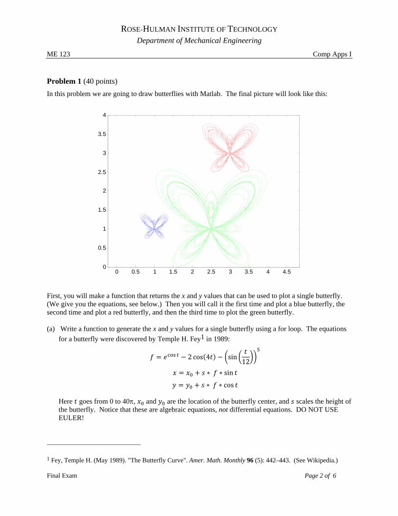
In this problem we are going to draw butterflies with Matlab. The final picture will look like this:
First, you will make a function that returns the x and y values that can be used to plot a single butterfly. (We give you the equations, see below.) Then you will call it the first time and plot a blue butterfly, the second time and plot a red butterfly, and then the third time to plot the green butterfly. (a) Write a function to generate the x and y values for a single butterfly using a for loop. The equations
for a butterfly were discovered by Temple H. Fey1 in 1989:
2 cos 4 sin12
∗ ∗ sin
∗ ∗ cos Here goes from 0 to 40, and are the location of the butterfly center, and scales the height of the butterfly. Notice that these are algebraic equations, not differential equations. DO NOT USE EULER!
1 Fey, Temple H. (May 1989). "The Butterfly Curve". Amer. Math. Monthly 96 (5): 442–443. (See Wikipedia.)
0 0.5 1 1.5 2 2.5 3 3.5 4 4.50
0.5
1
1.5
2
2.5
3
3.5
4

ROSE-HULMAN INSTITUTE OF TECHNOLOGY
Department of Mechanical Engineering
ME 123 Comp Apps I
Final Exam Page 3 of 6
The function statement should look like this:
function [x, y] = butterfly_function(tmin, tmax, dt, s, xo, yo); where dt is the sampling step.
(b) Write a main program called problem1.m that calls your function to generate the curve for the blue butterfly. It has tmin=0, tmax=40*pi, dt=0.001, s=0.1, x0=1, y0=1. In the main program, plot the butterfly with a blue line and add the commands
axis([0 4 0 4]) axis equal hold on
(This will make your plot have the same axes as the one on the previous page.)
(c) Add code to your main program to create a red butterfly with s=0.2, x0=3, y0=3, and a green butterfly with s=0.4, x0=2.5, y0=1. (That is, call your butterfly function with the new parameters and add additional plot commands to your main program. Even if you cannot get the butterfly function working correctly, show how you would have added this code to the main program.)
Instructions on posting these files to DFS are found on the last page.

ROSE-HULMAN INSTITUTE OF TECHNOLOGY
Department of Mechanical Engineering
ME 123 Comp Apps I
Final Exam Page 4 of 6
Problem 2 (60 points)
A dynamic system is described by the following set of equations in which t, time, is the independent variable.
0.04 1.2
0.25
The initial conditions are: 0 2.0, 0 0.0, and 0 0.0.
(a) Using Euler’s method, write a program called problem2.m which will calculate the values of , and for times from 0 to 15.
(b) Your program must then use the Matlab function, plot3, to draw a curve which represents the
system’s time history in the xyz space. (Use the Matlab help or documentation to learn more about plot3.) See below.
(c) Your program must calculate values of , and at time 15 which are accurate to two decimal
places, i.e. 0.01. Print the results to the command window with the following format:
fprintf(‘At time 15.0, x = %6.2f y = %6.2f z = %6.2f\n’, x(end),y(end),z(end)) (Note: x(end) prints the last entry in a vector.)
Instructions on posting your files to DFS are found on the last page.
-3-2
-10
12
3
-3
-2
-1
0
1
2
30
0.5
1
1.5
2
2.5
3
3.5
4
x
Solution to Dynamic System
y
z

ROSE-HULMAN INSTITUTE OF TECHNOLOGY
Department of Mechanical Engineering
ME 123 Comp Apps I
Final Exam Page 5 of 6
Partner/Team Evaluation for ME123 Projects
Project 1: (Optimize Robot Object Pickup and Binning, simulation)
Name of Partner:
Portion of the work on the project completed by you _____ % by your partner _____%
Comments:
Project 2: (Pick up and bin objects by color with actual robot)
Name of Partner:
Portion of the work on the project completed by you _____ % by your partner _____%
Comments:
Project 3: (Draw logo with a robot)
Name of Partner:
Portion of the work on the project completed by you _____ % by your partner _____%
Comments:

ROSE-HULMAN INSTITUTE OF TECHNOLOGY
Department of Mechanical Engineering
ME 123 Comp Apps I
Final Exam Page 6 of 6
When you are done, create a folder on your laptop called lastname_firstname. Put all of your m-files in this folder. (There should be at least three files: butterfly_function.m, problem1.m, and problem2.m. If you created other functions be sure to include them as well.) Before you submt, run your code in the new folder to make sure all the necessary functions are included there. Post your folder to the correct location on DFS:
1. Double-click on “Documents” on your laptop. 2. Double-click on “DFS Root” on the left column. 4. Double-click on Academic Affairs. 5. Double-click on ME. 6. Double-click on ME123. 7. Double-click on Exams. 8. Double-click on the folder with your section number. 9. Copy and paste your lastname_firstname folder to this location.

ROSE-HULMAN INSTITUTE OF TECHNOLOGY
Department of Mechanical Engineering
ME 123 Comp Apps I
Final Exam Page 1 of 4
FINAL EXAM – MATLAB Programming
NAME ___________________________________________
SECTION NUMBER _______________________________
CAMPUS MAILBOX NUMBER _____________________
EMAIL ADDRESS [email protected]
Problem 1 _________________/ 60
Problem 2 _________________/ 20
Problem 3 _________________/ 20
Total _____________________/ 100

ROSE-HULMAN INSTITUTE OF TECHNOLOGY
Department of Mechanical Engineering
ME 123 Comp Apps I
Final Exam Page 2 of 4
Problem 1 (60 points)
A simple robotic arm can be modeled as a pendulum, like in the picture to the right. Let be the angular displacement of the pendulum counterclockwise from the downward position, and denote the angular velocity by . There is damping in the pivot, and a force is applied horizontally to the lumped mass at the end of the pendulum.
The equations governing the behavior of a particular pendulum are as follows:
dt
0.4 20 sin cos
dt
where the units for and are rad and rad/s, respectively, and time is in seconds. Suppose the applied force is such that
0 when 0
2 when 0.
The initial conditions for the pendulum are
0 4 rad/s
0 0 rad.
Complete the following:
1. (40 points) Use MATLAB to plot the pendulum’s angular displacement as a function of time , starting at 0 s and ending at 4 s. Use a time step Δ 0.01 s. Be sure to properly label your axes and to include a title.
2. (20 points) Determine the values of and at 1.737s. Note that your time vector does not have this exact value of time in it. Print these values to the screen using the following format:
Angular displacement at t = 1.737 s is X.XXX rad. Angular velocity at t = 1.737 s is X.XXX rad/s.
Name your m-file lastname_firstname_problem1.m (all lower case). Instructions on posting this file to DFS are found on Page 4.

ROSE-HULMAN INSTITUTE OF TECHNOLOGY
Department of Mechanical Engineering
ME 123 Comp Apps I
Final Exam Page 3 of 4
Problem 2 (20 points)
In this problem, you will be asked to write a MATLAB function which determines the volume of fluid, with a variable height h, contained in a feeding trough with a geometry depicted below:
The radius of the semi-circular base is 0.75 m. Your function should perform the following tasks in an efficient way:
receive only one input variable h from a main calling code.
internally define a feeding trough height H of 3 m, a trough length L of 5 m, and a semi-circular radius R of
0.75 m.
check if the input is physically meaningful, i.e. fits within the physical constraints of the feeding trough. If
not, return a zero value for the output volume and print a warning message to the user:
Error message: Your input fluid level is outside the physical range!
return the fluid volume for the given fluid level h, in cubic meters, for the two cases:
Fluid level is in the semi-circular base:
2 sin 2
2V R L
where is in radians and defined by
1cos 1h
R
Fluid level is in the rectangular top:
2
22
RV R L h R L
print out the result in the following format:
The total fluid volume is x.xxxxxe+xxx cubic meters at a fluid level of x.xxxe+xxx meters. Name your function lastname_firstname_problem2.m (all lower case). Instructions on posting this file to DFS are found on Page 4.
L = 5 m
hR
H = 3 m
Side View End View
ROSE-HULMAN INSTITUTE OF TECHNOLOGY
Department of Mechanical Engineering
ME 123 Comp Apps I
Final Exam Page 4 of 4
Problem 3 (20 points)
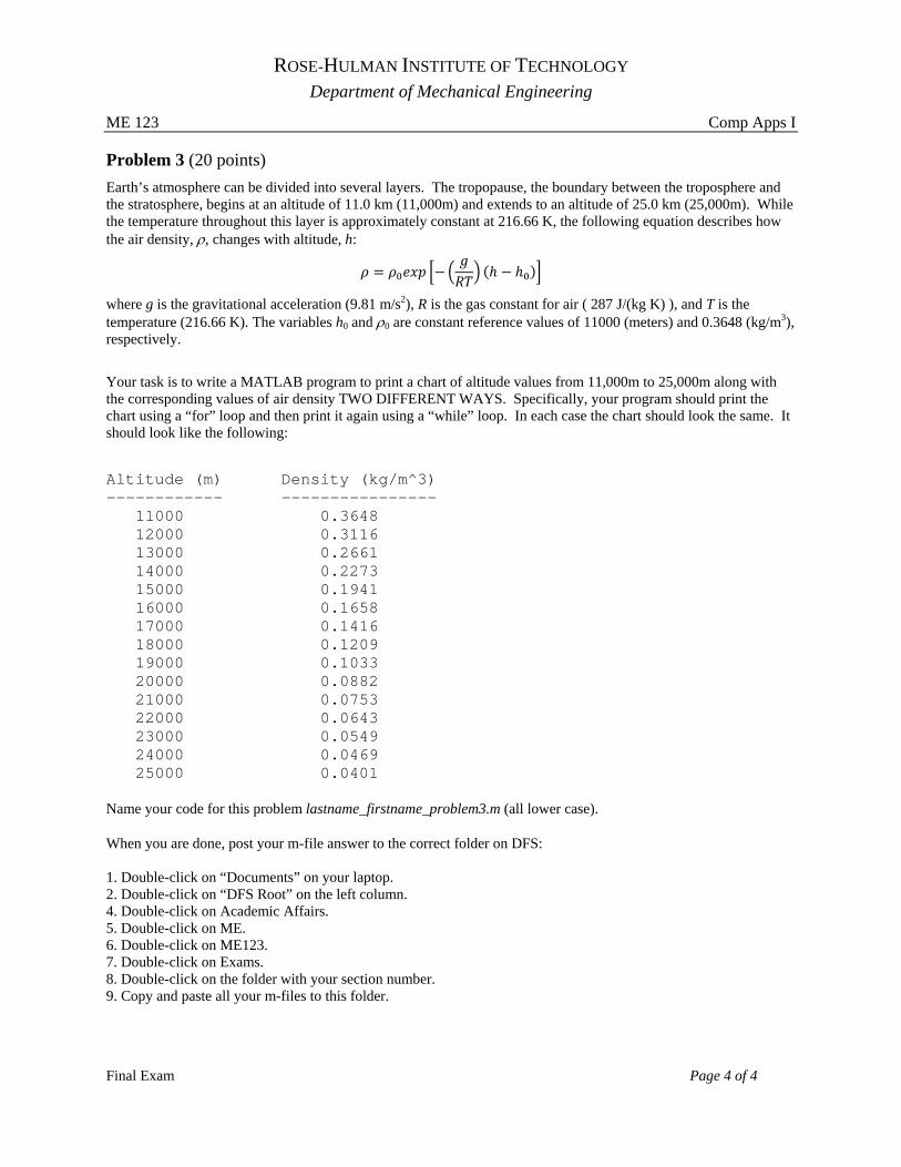
Earth’s atmosphere can be divided into several layers. The tropopause, the boundary between the troposphere and the stratosphere, begins at an altitude of 11.0 km (11,000m) and extends to an altitude of 25.0 km (25,000m). While the temperature throughout this layer is approximately constant at 216.66 K, the following equation describes how the air density, , changes with altitude, h:
where g is the gravitational acceleration (9.81 m/s2), R is the gas constant for air ( 287 J/(kg K) ), and T is the temperature (216.66 K). The variables h0 and 0 are constant reference values of 11000 (meters) and 0.3648 (kg/m3), respectively.
Your task is to write a MATLAB program to print a chart of altitude values from 11,000m to 25,000m along with the corresponding values of air density TWO DIFFERENT WAYS. Specifically, your program should print the chart using a “for” loop and then print it again using a “while” loop. In each case the chart should look the same. It should look like the following:
Altitude (m) Density (kg/m^3) ------------ ---------------- 11000 0.3648 12000 0.3116 13000 0.2661 14000 0.2273 15000 0.1941 16000 0.1658 17000 0.1416 18000 0.1209 19000 0.1033 20000 0.0882 21000 0.0753 22000 0.0643 23000 0.0549 24000 0.0469 25000 0.0401
Name your code for this problem lastname_firstname_problem3.m (all lower case).
When you are done, post your m-file answer to the correct folder on DFS: 1. Double-click on “Documents” on your laptop. 2. Double-click on “DFS Root” on the left column. 4. Double-click on Academic Affairs. 5. Double-click on ME. 6. Double-click on ME123. 7. Double-click on Exams. 8. Double-click on the folder with your section number. 9. Copy and paste all your m-files to this folder.

ROSE-HULMAN INSTITUTE OF TECHNOLOGY
Department of Mechanical Engineering
ME 123 Comp Apps I
Exam 3 Page 1 of 4
EXAM 4 – Matlab Programming
NAME ___________________________________________
SECTION NUMBER _______________________________
CAMPUS MAILBOX NUMBER _____________________
EMAIL ADDRESS [email protected]
Problem 1 _________________/60
Problem 2 _________________/20
Problem 3 _________________/20
Total _____________________/100

ROSE-HULMAN INSTITUTE OF TECHNOLOGY
Department of Mechanical Engineering
ME 123 Comp Apps I
Exam 3 Page 2 of 4
Problem 1 (60 points)
A shock absorber system can be modeled as a mass, a spring and a damper as in the picture below. The mass can only move back and forth in the x-direction. Its displaced position will be designated by x, and its velocity by v.
An engineer has derived the following equations to describe the behavior of the system. (Assume that we are using SI units, with kilograms, meters, and seconds.)
2.400 4.000
At time zero, an impulse loading is supplied to the system. The effect is to give the mass an instantaneous velocity in the positive x-direction. The initial conditions may then be written as follows.
0 2.000 0 0.000
The resulting motion of the mass is an exponentially decaying sine curve. The mass will move to the right and reach a maximum position xmax at time tmax. The mass will then move back to the left, passing through the starting point and reach a minimum (maximum negative valued) position xmin at time tmin. Further oscillations of decreasing amplitude will follow.
1. (40 points) Use Matlab to plot the value of displaced position x as a function of time starting at time 0 and ending at a time of 5.
2. (20 points) The program should print out the values of xmax, tmax, xmin and txmin with statements using the following format.
Maximum displacement of X.XXX meters occurs at time X.XXX seconds.
Minimum displacement of -X.XXX meters occurs at time X.XXX seconds.
To get full credit in Part 2, every digit reported must be correct. In other words, your program must be accurate enough to calculate values which will correctly round to three decimal places.
Name your m-file lastname_firstname_problem1.m Instructions on posting this file to DFS are found on Page 4.
spring
damper
mass x, v
x=0 starting point
ROSE-HULMAN INSTITUTE OF TECHNOLOGY
Department of Mechanical Engineering
ME 123 Comp Apps I
Exam 3 Page 3 of 4
R
R L
Level of water in the tank is given by “h” h
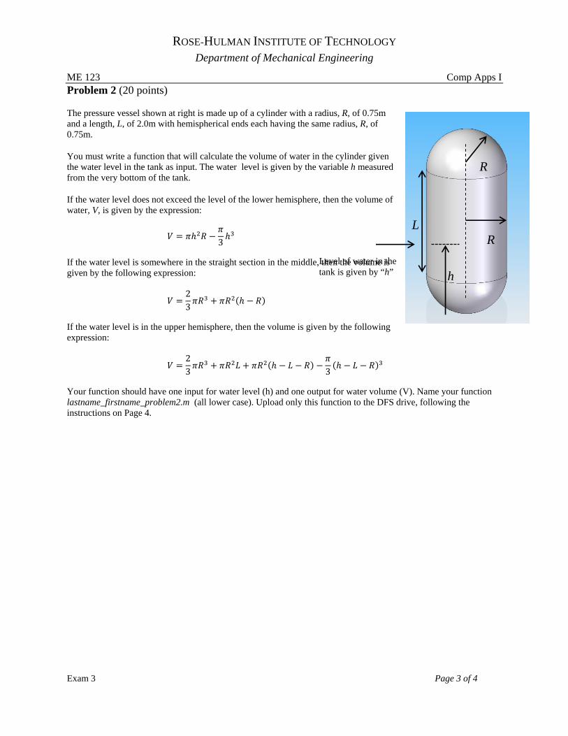
Problem 2 (20 points)
The pressure vessel shown at right is made up of a cylinder with a radius, R, of 0.75m and a length, L, of 2.0m with hemispherical ends each having the same radius, R, of 0.75m.
You must write a function that will calculate the volume of water in the cylinder given the water level in the tank as input. The water level is given by the variable h measured from the very bottom of the tank.
If the water level does not exceed the level of the lower hemisphere, then the volume of water, V, is given by the expression:
3
If the water level is somewhere in the straight section in the middle, then the volume is given by the following expression:
23
If the water level is in the upper hemisphere, then the volume is given by the following expression:
23 3
Your function should have one input for water level (h) and one output for water volume (V). Name your function lastname_firstname_problem2.m (all lower case). Upload only this function to the DFS drive, following the instructions on Page 4.
ROSE-HULMAN INSTITUTE OF TECHNOLOGY
Department of Mechanical Engineering
ME 123 Comp Apps I
Exam 3 Page 4 of 4
x values
y va
lues
contour plot of z = sin(x)*sin(y)
0 1 2 3 4 5 60
1
2
3
4
5
6
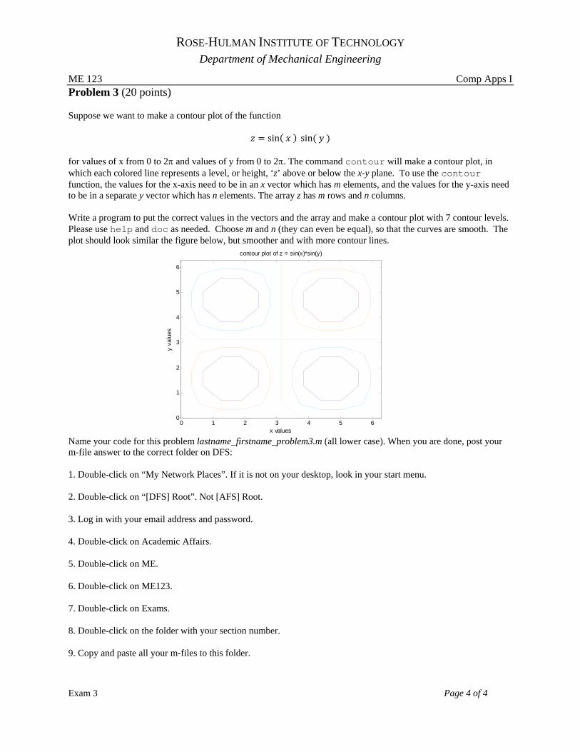
Problem 3 (20 points)
Suppose we want to make a contour plot of the function
sin sin
for values of x from 0 to 2 and values of y from 0 to 2. The command contour will make a contour plot, in which each colored line represents a level, or height, ‘z’ above or below the x-y plane. To use the contour function, the values for the x-axis need to be in an x vector which has m elements, and the values for the y-axis need to be in a separate y vector which has n elements. The array z has m rows and n columns.
Write a program to put the correct values in the vectors and the array and make a contour plot with 7 contour levels. Please use help and doc as needed. Choose m and n (they can even be equal), so that the curves are smooth. The plot should look similar the figure below, but smoother and with more contour lines.
Name your code for this problem lastname_firstname_problem3.m (all lower case). When you are done, post your m-file answer to the correct folder on DFS:
1. Double-click on “My Network Places”. If it is not on your desktop, look in your start menu.
2. Double-click on “[DFS] Root”. Not [AFS] Root.
3. Log in with your email address and password.
4. Double-click on Academic Affairs.
5. Double-click on ME.
6. Double-click on ME123.
7. Double-click on Exams.
8. Double-click on the folder with your section number.
9. Copy and paste all your m-files to this folder.
ROSE-HULMAN INSTITUTE OF TECHNOLOGY
Department of Mechanical Engineering
ME123 Computer Applications I
EXAM 1 – WRITTEN PORTION
NAME ___________________________________________
SECTION NUMBER _______________________________
CAMPUS MAILBOX NUMBER _____________________
EMAIL ADDRESS [email protected]
Multiple Choice /40
Coding Problem /60
Total /100

ROSE-HULMAN INSTITUTE OF TECHNOLOGY
Department of Mechanical Engineering
ME123 Computer Applications I
ALL OF THESE PROBLEMS HAVE EQUAL WEIGHT
USE MATLAB SYNTAX FOR ALL PROGRAMS AND COMMANDS YOU WRITE
Problem 1: Write a short program using a for…end loop to find the sum of the squares of the numbers from 5 to 10. Assign the answer to a variable called total. You do not need to print the answers with fprintf. Problem 2: Write a short program using a for…end loop to find the square roots of the numbers 0, 10, 20…200. You do not need to print the answers with fprintf. Problem 3: Write a short program using a for…end loop to put the angles 0, 10, 20…90 into an array called ‘angle_array’. The array should have 10 rows and 1 column. You do not need to print the answers with fprintf. Problem 4: Circle ALL of the file names that would be appropriate to use in Matlab. Appropriate files names will run and not result in errors.
a) Lab 1 task 2.m b) 1sttaskforlab1.m c) plot.m d) MyName_4.m e) plot_lab1.m f) lecture‐2‐ex‐3.m
ROSE-HULMAN INSTITUTE OF TECHNOLOGY
Department of Mechanical Engineering
ME123 Computer Applications I
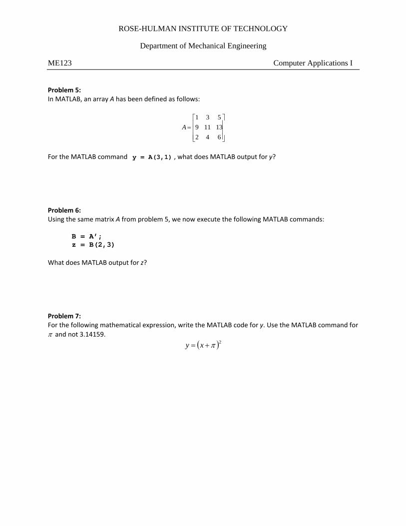
Problem 5: In MATLAB, an array A has been defined as follows:
⎥⎥⎥
⎦
⎤
⎢⎢⎢
⎣
⎡=
642
13119
531
A
For the MATLAB command y = A(3,1) , what does MATLAB output for y? Problem 6: Using the same matrix A from problem 5, we now execute the following MATLAB commands:
B = A’; z = B(2,3)
What does MATLAB output for z? Problem 7: For the following mathematical expression, write the MATLAB code for y. Use the MATLAB command for π and not 3.14159.
( )2π+= xy

ROSE-HULMAN INSTITUTE OF TECHNOLOGY
Department of Mechanical Engineering
ME123 Computer Applications I
Problem 8: When we run the MATLAB program shown below, an error statement appears in the Command window. Here’s the program:
% exampleProgram.m % % This program produces an mx1 array of angles named % degrees and an mx1 array of the sines of the angles % named sineAngle. for angle = 0 : pi/10 : 2*pi degrees(row,1) = angle*180/pi; sineAngle(row,1) = sin(angle); row = row + 1; end % last line
Here’s the error statement:
??? Undefined function or variable 'row'.
Error in ==> exampleProgram at 8 degrees(row,1) = angle*180/pi;
Modify the program to correct the error.

ROSE-HULMAN INSTITUTE OF TECHNOLOGY
Department of Mechanical Engineering
ME123 Computer Applications I
Problem 9: Consider the following piece of code:
fred = 1; for index = 1:3:8 fred = fred*index; end fred
What result will MATLAB produce in the Command window? (Circle one.)
a) fred = 1 b) fred = 7 c) fred = 21 d) fred = 28 e) fred = 280 f) Other: ________________
Problem 10: Consider the following piece of code:
index = 0; for count = 3:-1:1 index = index + 1; A(1,index) = count; end A
What is A after the code is executed? (Circle one.)
a) A = 1 2 3
b) A = 3 2 1
c) A = 123
d) A = 321
e) A = 6
f) Other: ______________

ROSE-HULMAN INSTITUTE OF TECHNOLOGY
Department of Mechanical Engineering
ME 123 Computer Applications I
Proposal for Exam 1 Page 1 of 1
EXAM 1 – COMPUTER PORTION
Put all of your code in one m-file and name it: lastname_firstname.m (all lower case). Include your name, section number, and CM number in the header section of your code. There should be no output other than what is asked for. Problem (60 pts) Download the Excel spreadsheet named “rate.xls” from the course web page at http://www.rose-hulman.edu/ME123/courseware.shtml. The file contains one column of annual investment rates (as percentages) for the years 1993 through 2007 (15 years total). Write a MATLAB code to: a) Read in the rate data stored in the Excel spreadsheet. Print the year and the rate for that year to a text file
lastname_firstname1.txt, where lastname and firstname should be replaced by your last and first names, respectively. Do not forget to use the fclose command in your code. The first 3 lines of the text file should be: Year Rate (percent) 1993 11.28 1994 -0.06 .. .. .. ..
b) Assume you started with $1000 in an investment account at the end of 1992. Use the annual investment rates provided, determine the balance in the account at the end of each year from 1992 through 2007, with no withdrawal. Print your end-of-year balances to the screen with the first 3 lines displaying the following format: Year Balance 1992 $1000.00 1993 $1112.80 .. .. .. ..
c) Plot the rates of return from 1993 to 2007 as a function of the year. Properly label both axes, and give your plot a title.
When you are done, post your m-file to the correct folder:
1. Double-click on “My Network Places”. If it is not on your desktop, look in your start menu. 2. Double-click on “[DFS] Root”. Not [AFS] Root. 3. Log in with your email address and password. 4. Double-click on Academic Affairs. 5. Double-click on ME. 6. Double-click on ME123. 7. Double-click on Exams. 8. Double-click on the folder with your section number. 9. Copy and paste your m-file to this folder.
NOTE: All programming must stop at 8:30pm. You will have a few minutes after that to post your file if you need that time.