Final Control Element (Actuator ) Gs Process Controller L...

Colorado School of Mines CHEN403 Stability Feedback Control Systems

John Jechura ([email protected]) - 1 - © Copyright 2017

April 23, 2017

Stability Analysis of Feedback Control Systems

Stability Analysis of Feedback Control Systems ......................................................................................... 1

Introduction ................................................................................................................................................................ 1

Routh-Hurwitz Stability Criterion ..................................................................................................................... 2

Example #1 ............................................................................................................................................................. 4

Direct Substitution ................................................................................................................................................... 6

Example #1 by Direct Substitution .............................................................................................................. 6

Example with P & PI Control .......................................................................................................................... 7

Example with Dead Time .............................................................................................................................. 11

Root-Locus Analysis ............................................................................................................................................. 13

Introduction

+-

y

LG s

cG s ++ pG s

M

L

spy aG s

C

mG smy

Controller

Process

Final Control

Element (Actuator)

Measuring Element

Remember that for the generalized closed-loop system shown above the overall transfer function is:

1 1

p f c dsp

p f c m p f c m

G G G Gy y d

G G G G G G G G

where: 1

p f c

sp

p f c m

G G GG

G G G G and

1d

load

p f c m

GG

G G G G



April 23, 2017

Review the section Poles & Zeros in the notes Transfer Functions for a discussion of process stability. The definition of stability we will use for bounded input, bounded output stability is:

A dynamic system is considered stable if for every bounded input it produces a bounded output, regardless of its initial state.

The stability will be dictated by the characteristic poles of the transfer functions spG and

loadG . The characteristic equation to give these poles is the same (since the denominator is the same): 1 0p f c mG G G G .

Note that if the control is cut right before the comparator, we get the open loop transfer function:

mp f c m OL

sp

yG G G G G

y

so the characteristic equation can be written as: 1 0OLG .

For example, a process with a transfer function 1/( 1)pG s is unstable since it has a positive pole 1s . However, let’s put in a P controller with 1m fG G . Then, the closed loop characteristic equation will be:

11 1 1 0 1 0

1c cK s K

s.

Now, the pole is at 1 cs K . This will be a stable dynamic system if Re( ) 0s s , or: 1 0 1c cK K .

Routh-Hurwitz Stability Criterion

We do not necessarily need to know the poles to determine stability — just the knowledge of which side of the complex plane the poles lie may be enough. We can set up a Routh array to determine this. The steps are:

• Express the characteristic equation as an expanded polynomial:



April 23, 2017

1

1 1 01 n np f c m n nG G G G a s a s a s a .

where 0 0a . This subscript notation is different from many other texts that

use:

1

0 1 11 n np f c m n nG G G G a s a s a s a .

• If any of the coefficients are negative, then there is at least one root with a

positive real part and the system is unstable.

• Set up a table that looks like the following:

Row

1 an an-2 an-4 an-6

2 an-1 an-3 an-5 an-7

3 b1 b2 b3

4 c1 c2 c3

5 d1 d2

6 e1 e2

where the elements are found from equations like:

1 2 3 3

1 2

1 1

n n n n n nn

n n

a a a a a ab a

a a

1 4 5 5

2 4

1 1

n n n n n nn

n n

a a a a a ab a

a a

1 3 1 2 1 2

1 3

1 1

nn

b a a b a bc a

b b

1 5 1 3 1 3

2 5

1 1

n n nn

b a a b a bc a

b b

The rule is to look at the square matrix above the element to be calculated. Use the values from column 1 & the column just to the right of the element of interest. Multiply the off diagonal terms, subtract the product of the diagonal terms, and divide by the element just above. So, for example, term 2d will be:

1 3 1 3 1 32 3

1 1

c b b c b cd b

c c …



April 23, 2017

• If all of the elements in the 1st column are positive, then the system is stable. • If some of the elements in the 1st column are negative, the number of roots with

a positive real part will be equal to the number of sign changes in the 1st column.

We can use the criteria to pick valid controller parameters that keep the system stable.

Example #1

In the following system, determine the value of the gain that makes the system unstable if (a) 0.25 minD and (b) 0.5 minD . Use the following data:

250 lb/minm

62.5 lb/ft³

1 4 ft³V

2 5 ft³V

3 6 ft³V

ˆ 1 Btu/lb FpC

The energy balance around each tank will be:

1 1

ˆˆ ˆˆ ˆi i

ii i i i p p i i i

d V H dTmH mH Q V C mC T T Q

dt dt

So, it terms of deviation variables & taking the Laplace transform we get 1st order systems of the form:

1

1

1 1

q

i i i

i i

KT T Q

s s where

i

i

V

m &

1ˆq

p

KmC

and where 2 3 0Q Q since there are no heaters in these tanks. The following information block diagram shows the feedback control system.



April 23, 2017

+-

3T

1

1

1s

cG s ++

2

1

1s 3

1

1s

2T

1T

0T

spT

1 1

qK

s

Q

The system parameters will be:

1

1 10.004 F/(Btu/min)

ˆ 250 1p

KmC

11

62.5 41.00 min

250

V

m

22

62.5 51.25 min

250

V

m

33

62.5 61.50 min

250

V

m

The characteristic equation will be:

11 2 3

1 2 3

1 11 1 1

1 1 1

0.004 1 11 1

1 1.25 1 1.50 1

c f c D

c D

KG G G G G K s

s s s

K ss s s

1 1.25 1 1.50 1 0.004 1 0c Ds s s K s

3 21.875 4.625 3.75 1 0.004 0.004 0D c cs s s K s K

The Routh array will be:



April 23, 2017

Row 1 2

1 1.875 3.75 0.004 c DK

2 4.625 1 0.004 cK

3 4.625 3.75 0.004 1.875 1 0.004

4.625c D cK K

4 1 0.004 cK

The important element is:

4.625 3.75 0.004 1.875 1 0.004

3.345 0.004 0.001624.625c D c

c D c

K KK K

So, the system will be stable as long as: 3.345 0.004 0.00162 0c D cK K

0.00162 0.004 3.345D cK

So: for 0.25D , 0.00062 3.345 5380c cK K — this case has conditional stability. For 0.50D , 0.00038 3.345 8800c cK K — this case has unconditional stability.

Direct Substitution

The direct substitution method can give both the ultimate values of the controller settings and the period of oscillation at the ultimate settings. It can also be applied to systems with dead time without having to make any approximations to the se term. The procedure is to substitute s j (where 1j ) and set the real & imaginary parts to zero. These expressions will give the ultimate values for (the frequency of oscillation at this stability limit) & the associated controller settings. A time delay term poses no problems since:

cos sinje j .

Example #1 by Direct Substitution For the previous example the characteristic equation was:

3 21.875 4.625 3.75 1 0.004 0.004 0D c cs s s K s K



April 23, 2017

Substituting s j :

3 2

1.875 4.625 3.75 1 0.004 0.004 0D c cj j j K j K

3 21.875 4.625 3.75 1 0.004 0.004 0D c cj j K j K

2 21 0.004 4.625 3.75 0.004 1.875 0c D cK j K

From the imaginary part:

2 2 3.75 0.0043.75 0.004 1.875 0

1.875D cu

D cu

KK

and from the real part:

2

2 4.625 11 0.004 4.625 0

0.004cu cuK K .

Or we can use the result from the imaginary part first:

3.75 0.0041 0.004 4.625 0

1.875D cu

cu

KK

4.625 0.0044.625 3.75

1 0.004 01.875 1.875

D cc

KK

4.625 0.004 4.625 3.750.004 1

1.875 1.875D

cuK

4.625 3.75 1.875 3,867

0.004 1.875 4.625 0.004 1.875 4.625cu

D D

K .

So, for 0.25D , 5380cuK which is what we found previously. Next, for 0.50D ,

8839cuK — it is not immediately obvious how to interpret that, but we know from the Routh array analysis that this is a lower limit on cK , so this case has unconditional stability.

Example with P & PI Control Let’s consider the following example where the actuator & measurement devices have non-negligible dynamics.



April 23, 2017

+- Y

5

10 1s

cG ++

10

10 1s

1

1s

L

R

1

1s

For this problem the characteristic equation will be:

1 1 101 0

1 1 10 1cG

s s s

2

1 10 1 10 0cs s G

3 210 21 12 1 10 0cs s s G

P Control – Routh Array Analysis. With P control, the characteristic equation is:

3 210 21 12 1 10 0cs s s K

and the Routh array is as follows:

Row 1 2

1 10 12

2 21 1 10 cK

3

10 1 10

1221

cK

4 1 10 cK

Notice that the restriction on cK from the 4th row is exactly the same as the restriction on

cK from the polynomial’s coefficients, namely

1

1 10 010

c cK K .

This is not really a restriction since we are considering only positive values for the controller gain.



April 23, 2017

However, the 3rd row does give a restriction on cK :

10 1 10 12 21 1012 0 2.42

21 100c

c

KK .

There are two important features to the result, (1) the value of the controller gain that will be on the edge of stability and (2) whether this value is a maximum controller gain to be used or a minimum. In this case we see that the ultimate controller gain is a maximum – this is typical of P control – the gain can be small & the larger that it is made, the more likely the system will start going unstable. P Control – Direct Substitution Analysis. With P control, the characteristic equation with the substitution of s j is:

3 210 21 12 1 10 0cj j K

The imaginary part gives:

3 2 2 12 310 12 0 12 10 0 2

10 10u u u u u u

and the real part gives:

22

1221 1

21 1 1021 1 10 0 2.4210 10

uu cu cK K

which is the same ultimate value as found by the Routh array analysis. The only difference between the two techniques is that we are not told whether this cuK value is an upper or lower limit on cK . PI Control – Routh Array Analysis. With PI control, the characteristic equation is:

3 2 110 21 12 1 10 1 0c

I

s s s Ks

4 3 2 1010 21 12 1 10 0c

c

I

Ks s s K s

and the Routh array is as follows:



April 23, 2017

Row 1 2 3

1 10 12

10 c

I

K

2 21 1 10 cK

3

10 1 10

1221

cK

10 c

I

K

4

1021

1 1010 1 10

1221

c

Ic

c

K

KK

5

10 c

I

K

Here the 3rd row gives us the same restriction on cK as the P control situation. Now we also have a restriction on the integral time from the 4th row:

1021

44101 10 0

10 1 10 1 10 242 10012

21

c

cIc I

c c c

K

KK

K K K.

There are two things to note here: (1) the ultimate value of I that leads to instability is a minimum value of integral time & (2) the actual value will depend upon whatever value of controller gain is used. That idea that the integral time can be reduced until instability occurs makes intuitive sense, since very large values of I “turns off” the integral action in the PI controller. One rule-of-thumb states that the cK value chosen for PI control should be ½ the ultimate value from P control. Using this criteria, cK here should be 1.21; however, we’ll use 1cK to simplify the math. Then the values of I that lead to a stable system are:

44102.82

11 142I .

PI Control – Direct Substitution Analysis. With PI control, the characteristic equation using

1cK and with the substitution of s j is:

4 3 2 1010 21 12 11 0

I

j j .



April 23, 2017

The imaginary part gives:

3 2 2 11 1121 11 0 11 21 0

21 21u u u u u u

and the real part gives:

4 2

22 4

10 10 1010 12 0 2.82

12 10 11 1112 10

21 21

u u Iu

Iu u u

which is the same ultimate value as found by the Routh array analysis. Again, the only difference between the two techniques is that we are not told whether this Iu value is an

upper or lower limit on I .

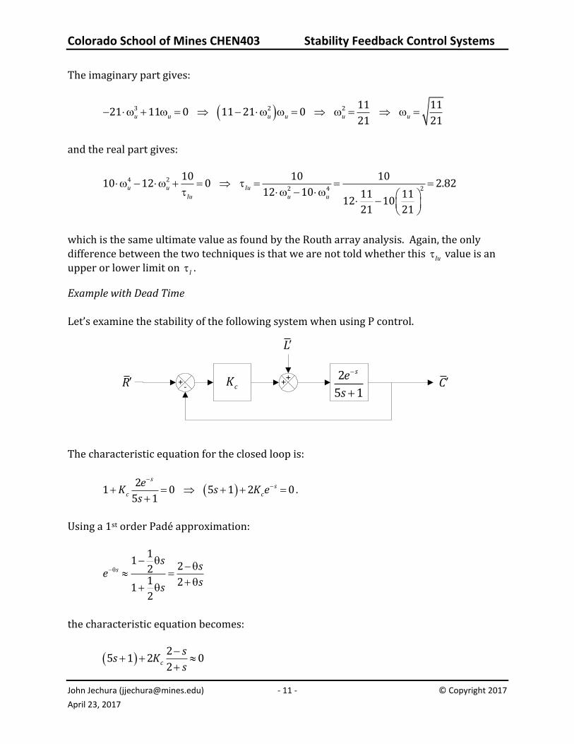
Example with Dead Time Let’s examine the stability of the following system when using P control.

+-

R C

2

5 1

se

scK +

+

L

The characteristic equation for the closed loop is:

21 0 5 1 2 0

5 1

ss

c c

eK s K e

s.

Using a 1st order Padé approximation:

11

221 212

ss

se

ss

the characteristic equation becomes:

25 1 2 0

2c

ss K

s



April 23, 2017

5 1 2 2 2 0cs s K s

25 11 2 2 2 0cs s K s

25 11 2 2 4 0c cs K s K .

The first limit to stability is the coefficient on the s term. For it to remain positive, then: 11 2 0 5.5c cK K .

Next, we’ll do the full Routh array analysis. The Routh array will be:

Row 1 2

1 5 2 4 cK

2 11 2 cK

3 2 4 cK

The stability limit is still controlled by the same coefficient. Now, let’s use the direct substitution method. The characteristic equations becomes:

5 1 2 0jcj K e

5 1 2 cos sin 0cj K j

1 2 cos 5 2 sin 0c cK j K .

The ultimate values can be determined by setting each part equal to zero & doing some algebraic manipulation:

11 2 cos 0

2cosc cuK K

and:

sin5 2 sin 0 5 0

cos

5 tan 0

cuK

The value for must be solved numerically & then substituted in to get cuK . When doing this, we find 1.6887 and 4.251cuK .

Note that the use of 1st order overestimates the ultimate value. One can use higher order

approximations to determine what order approximations will give good estimates to cuK . The following table shows estimates using various order Padé approximations (the



April 23, 2017

calculations were performed using Mathematica). Notice that the a values from the approximate tranfer functions very quickly approach the exact value from the direct substitution method.

Order Padé Approximation

cuK

1st 5.5 2nd 4.289 3rd 4.252

Exact 4.251

Root-Locus Analysis

Can plot in the complex plane the values of the roots of the characteristic equation as the

controller parameter change. These root loci plots can be useful to determine characteristics of the response of the system. For example, for two tanks in series with P control, assuming 1f mG G , then:

1 21 1

p

p

KG

s s and c cG K

and the characteristic equation is:

1 2

1 1 01 1

c p

c p

K KG G

s s

1 21 1 0c ps s K K

21 2 1 2 1 0c ps s K K

so the roots of this equation are given by:

2

1 2 1 2 1 2

1 2

1 2

2

1 2 1 2 1 2

1 2

4 1,

2

4

2

c p

c p

K Kp p

K K

From this, you can make the following observations:

• When 0cK , then:



April 23, 2017

2

1 2 1 2 1 2 1 2

1 2

1 2 1 2 1 2

1 1, ,

2 2p p

the “standard” roots for a non-interacting series of processes.

• We can get a critically damped response when the roots are repeated, or when:

2

2 1 2

1 2 1 2

1 2

4 04

c p c

p

K K KK

So, this means that the system will be overdamped when:

2

2 1 2

1 2 1 2

1 2

4 04

c p c

p

K K KK

Furthermore, for these values of cK the poles will remain negative real. • We can get an underdamped response when:

2

2 1 2

1 2 1 2

1 2

4 04

c p c

p

K K KK

The poles are then given by:

2

1 2 1 21 21 2

1 2 1 2

4,

2 2

c pK Kp p i

The real portion of these roots remain negative, whereas the imaginary part gets bigger and bigger as cK increases.

These types of plots are more instructive for more complicated systems — for example, see the plot on page 265 of SEM. This plot shows that as cK increases, an underdamped system results. However, the real portion of the complex conjugate roots also increases, going positive at 30cK . So, the gain must be kept below this value.

Final Control Element (Actuator ) Gs Process Controller L...

Documents

Transcript of Final Control Element (Actuator ) Gs Process Controller L...