Filter Design
345
Filter Design Toolbox 4 User’s Guide
-
Upload
oguz-cevik -
Category
Documents
-
view
105 -
download
2
Transcript of Filter Design

Filter Design Toolbox 4User’s Guide
How to Contact The MathWorks
www.mathworks.com Webcomp.soft-sys.matlab Newsgroupwww.mathworks.com/contact_TS.html Technical Support
[email protected] Product enhancement [email protected] Bug [email protected] Documentation error [email protected] Order status, license renewals, [email protected] Sales, pricing, and general information
508-647-7000 (Phone)
508-647-7001 (Fax)
The MathWorks, Inc.3 Apple Hill DriveNatick, MA 01760-2098For contact information about worldwide offices, see the MathWorks Web site.
Filter Design Toolbox User’s Guide
© COPYRIGHT 2000–2007 by The MathWorks, Inc.The software described in this document is furnished under a license agreement. The software may be usedor copied only under the terms of the license agreement. No part of this manual may be photocopied orreproduced in any form without prior written consent from The MathWorks, Inc.
FEDERAL ACQUISITION: This provision applies to all acquisitions of the Program and Documentationby, for, or through the federal government of the United States. By accepting delivery of the Program orDocumentation, the government hereby agrees that this software or documentation qualifies as commercialcomputer software or commercial computer software documentation as such terms are used or definedin FAR 12.212, DFARS Part 227.72, and DFARS 252.227-7014. Accordingly, the terms and conditions ofthis Agreement and only those rights specified in this Agreement, shall pertain to and govern the use,modification, reproduction, release, performance, display, and disclosure of the Program and Documentationby the federal government (or other entity acquiring for or through the federal government) and shallsupersede any conflicting contractual terms or conditions. If this License fails to meet the government’sneeds or is inconsistent in any respect with federal procurement law, the government agrees to return theProgram and Documentation, unused, to The MathWorks, Inc.
Trademarks
MATLAB, Simulink, Stateflow, Handle Graphics, Real-Time Workshop, SimBiology,SimHydraulics, SimEvents, and xPC TargetBox are registered trademarks and TheMathWorks, the L-shaped membrane logo, Embedded MATLAB, and PolySpace aretrademarks of The MathWorks, Inc.
Other product or brand names are trademarks or registered trademarks of their respectiveholders.
Patents
The MathWorks products are protected by one or more U.S. patents. Please seewww.mathworks.com/patents for more information.

Revision HistoryMarch 2000 Online only New for Version 1.0September 2000 First printing Revised for Version 2.0 (Release 12)June 2001 Online only Revised for Version 2.1 (Release 12.1)July 2002 Online only Revised for Version 2.2 (Release 13)November 2002 Online only Revised for Version 2.5June 2004 Online only Revised for Version 3.0 (Release 14)October 2004 Online only Revised for Version 3.1 (Release 14SP1)March 2005 Online only Revised for Version 3.2 (Release 14SP2)September 2005 Online only Revised for Version 3.3 (Release 14SP3)March 2006 Online only Revised for Version 3.4 (Release 2006a)September 2006 Online only Revised for Version 4.0 (Release 2006b)March 2007 Online only Revised for Version 4.1 (Release 2007a)September 2007 Online only Revised for Version 4.2 (Release 2007b)


Contents
Designing a Filter — Process Overview
1Process Flow Diagram and Filter Design
Methodology . . . . . . . . . . . . . . . . . . . . . . . . . . . . . . . . . . . . 1-2Exploring the Process Flow Diagram . . . . . . . . . . . . . . . . . . 1-2Selecting a Response . . . . . . . . . . . . . . . . . . . . . . . . . . . . . . . 1-4Selecting a Specification . . . . . . . . . . . . . . . . . . . . . . . . . . . . 1-4Selecting an Algorithm . . . . . . . . . . . . . . . . . . . . . . . . . . . . . 1-6Customizing the Algorithm . . . . . . . . . . . . . . . . . . . . . . . . . 1-7Designing the Filter . . . . . . . . . . . . . . . . . . . . . . . . . . . . . . . 1-8Design Analysis . . . . . . . . . . . . . . . . . . . . . . . . . . . . . . . . . . . 1-9Realize or Apply the Filter to Input Data . . . . . . . . . . . . . . 1-10
Using the Filterbuilder GUI
2The Graphical Interface to Fdesign . . . . . . . . . . . . . . . . . 2-2
Introduction to Filterbuilder . . . . . . . . . . . . . . . . . . . . . . . . 2-2Filterbuilder Design Process . . . . . . . . . . . . . . . . . . . . . . . . 2-3Select a Response . . . . . . . . . . . . . . . . . . . . . . . . . . . . . . . . . 2-3Select a Specification . . . . . . . . . . . . . . . . . . . . . . . . . . . . . . 2-6Select an Algorithm . . . . . . . . . . . . . . . . . . . . . . . . . . . . . . . . 2-6Customize the Algorithm . . . . . . . . . . . . . . . . . . . . . . . . . . . 2-7Analyze the Design . . . . . . . . . . . . . . . . . . . . . . . . . . . . . . . . 2-9Realize or Apply the Filter to Input Data . . . . . . . . . . . . . . 2-9
Designing a FIR Filter Using filterbuilder . . . . . . . . . . . 2-11FIR Filter Design . . . . . . . . . . . . . . . . . . . . . . . . . . . . . . . . . 2-11
v

Digital Frequency Transformations
3Details and Methodology . . . . . . . . . . . . . . . . . . . . . . . . . . . 3-2
Overview of Transformations . . . . . . . . . . . . . . . . . . . . . . . . 3-2Selecting Features Subject to Transformation . . . . . . . . . . 3-6Mapping from Prototype Filter to Target Filter . . . . . . . . . 3-8Summary of Frequency Transformations . . . . . . . . . . . . . . 3-10
Frequency Transformations for Real Filters . . . . . . . . . 3-11Overview . . . . . . . . . . . . . . . . . . . . . . . . . . . . . . . . . . . . . . . . 3-11Real Frequency Shift . . . . . . . . . . . . . . . . . . . . . . . . . . . . . . . 3-11Real Lowpass to Real Lowpass . . . . . . . . . . . . . . . . . . . . . . . 3-13Real Lowpass to Real Highpass . . . . . . . . . . . . . . . . . . . . . . 3-15Real Lowpass to Real Bandpass . . . . . . . . . . . . . . . . . . . . . . 3-17Real Lowpass to Real Bandstop . . . . . . . . . . . . . . . . . . . . . . 3-19Real Lowpass to Real Multiband . . . . . . . . . . . . . . . . . . . . . 3-21Real Lowpass to Real Multipoint . . . . . . . . . . . . . . . . . . . . . 3-23
Frequency Transformations for Complex Filters . . . . . 3-26Overview . . . . . . . . . . . . . . . . . . . . . . . . . . . . . . . . . . . . . . . . 3-26Complex Frequency Shift . . . . . . . . . . . . . . . . . . . . . . . . . . . 3-26Real Lowpass to Complex Bandpass . . . . . . . . . . . . . . . . . . 3-28Real Lowpass to Complex Bandstop . . . . . . . . . . . . . . . . . . 3-30Real Lowpass to Complex Multiband . . . . . . . . . . . . . . . . . . 3-32Real Lowpass to Complex Multipoint . . . . . . . . . . . . . . . . . 3-34Complex Bandpass to Complex Bandpass . . . . . . . . . . . . . . 3-36
Using FDATool with Filter Design Toolbox
4Designing Advanced Filters in FDATool . . . . . . . . . . . . . 4-3
Overview of FDATool Features . . . . . . . . . . . . . . . . . . . . . . . 4-3Using FDATool with Filter Design Toolbox . . . . . . . . . . . . . 4-4Example — Design a Notch Filter . . . . . . . . . . . . . . . . . . . . 4-4
Switching FDATool to Quantization Mode . . . . . . . . . . . 4-7
vi Contents

Quantizing Filters in the Filter Design and AnalysisTool . . . . . . . . . . . . . . . . . . . . . . . . . . . . . . . . . . . . . . . . . . . . 4-10Setting Quantization Parameters . . . . . . . . . . . . . . . . . . . . 4-10Coefficients Options . . . . . . . . . . . . . . . . . . . . . . . . . . . . . . . 4-11Input/Output Options . . . . . . . . . . . . . . . . . . . . . . . . . . . . . . 4-13Filter Internals Options . . . . . . . . . . . . . . . . . . . . . . . . . . . . 4-15Filter Internals Options for CIC Filters . . . . . . . . . . . . . . . 4-19
Analyzing Filters with a Noise-Based Method . . . . . . . . 4-21Using the Magnitude Response Estimate Method . . . . . . . 4-21Comparing the Estimated and Theoretical Magnitude
Responses . . . . . . . . . . . . . . . . . . . . . . . . . . . . . . . . . . . . . 4-26Choosing Quantized Filter Structures . . . . . . . . . . . . . . . . . 4-26Converting the Structure of a Quantized Filter . . . . . . . . . 4-26Converting Filters to Second-Order Sections Form . . . . . . 4-27
Scaling Second-Order Section Filters . . . . . . . . . . . . . . . . 4-29Using the Reordering and Scaling Second-Order Sections
Dialog Box . . . . . . . . . . . . . . . . . . . . . . . . . . . . . . . . . . . . . 4-29Example — Scale an SOS Filter . . . . . . . . . . . . . . . . . . . . . . 4-31
Reordering the Sections of Second-Order SectionFilters . . . . . . . . . . . . . . . . . . . . . . . . . . . . . . . . . . . . . . . . . . 4-37Switching FDATool to Reorder Filters . . . . . . . . . . . . . . . . . 4-37
Viewing SOS Filter Sections . . . . . . . . . . . . . . . . . . . . . . . . 4-44Using the SOS View Dialog Box . . . . . . . . . . . . . . . . . . . . . . 4-44Example — View the Sections of SOS Filters . . . . . . . . . . . 4-47
Importing and Exporting Quantized Filters . . . . . . . . . . 4-51Overview and Structures . . . . . . . . . . . . . . . . . . . . . . . . . . . 4-51Example — Import Quantized Filters . . . . . . . . . . . . . . . . . 4-52To Export Quantized Filters . . . . . . . . . . . . . . . . . . . . . . . . . 4-53
Importing XILINX Coefficient (.COE) Files . . . . . . . . . . . 4-56Example — Import XILINX .COE Files . . . . . . . . . . . . . . . 4-56
Transforming Filters . . . . . . . . . . . . . . . . . . . . . . . . . . . . . . . 4-57FDATool Filter Transformation Capabilities . . . . . . . . . . . 4-57Original Filter Type . . . . . . . . . . . . . . . . . . . . . . . . . . . . . . . 4-58Frequency Point to Transform . . . . . . . . . . . . . . . . . . . . . . . 4-62
vii

Transformed Filter Type . . . . . . . . . . . . . . . . . . . . . . . . . . . . 4-63Specify Desired Frequency Location . . . . . . . . . . . . . . . . . . 4-63
Designing Multirate Filters in FDATool . . . . . . . . . . . . . . 4-68Introduction . . . . . . . . . . . . . . . . . . . . . . . . . . . . . . . . . . . . . . 4-68Switching FDATool to Multirate Filter Design Mode . . . . . 4-68Controls on the Multirate Design Panel . . . . . . . . . . . . . . . 4-69Quantizing Multirate Filters . . . . . . . . . . . . . . . . . . . . . . . . 4-80
Realizing Filters as Simulink Subsystem Blocks . . . . . . 4-83Introduction . . . . . . . . . . . . . . . . . . . . . . . . . . . . . . . . . . . . . . 4-83About the Realize Model Panel in FDATool . . . . . . . . . . . . . 4-83
Getting Help for FDATool . . . . . . . . . . . . . . . . . . . . . . . . . . 4-88The What’s This? Option . . . . . . . . . . . . . . . . . . . . . . . . . . . 4-88Additional Help for FDATool . . . . . . . . . . . . . . . . . . . . . . . . 4-88
Adaptive Filters
5Introducing Adaptive Filtering . . . . . . . . . . . . . . . . . . . . . 5-2
Overview of Adaptive Filters and Applications . . . . . . . 5-4Adaptive Filtering Methodology . . . . . . . . . . . . . . . . . . . . . . 5-4Choosing an Adaptive Filter . . . . . . . . . . . . . . . . . . . . . . . . . 5-6System Identification . . . . . . . . . . . . . . . . . . . . . . . . . . . . . . 5-7Inverse System Identification . . . . . . . . . . . . . . . . . . . . . . . . 5-8Noise or Interference Cancellation . . . . . . . . . . . . . . . . . . . . 5-9Prediction . . . . . . . . . . . . . . . . . . . . . . . . . . . . . . . . . . . . . . . . 5-9
Adaptive Filters in Filter Design Toolbox . . . . . . . . . . . . 5-11Overview of Adaptive Filtering in Filter Design Toolbox . . 5-11Algorithms . . . . . . . . . . . . . . . . . . . . . . . . . . . . . . . . . . . . . . . 5-11Using Adaptive Filter Objects . . . . . . . . . . . . . . . . . . . . . . . 5-14
Examples of Adaptive Filters That Use LMSAlgorithms . . . . . . . . . . . . . . . . . . . . . . . . . . . . . . . . . . . . . . 5-15LMS Methods Available in Filter Design Toolbox . . . . . . . . 5-15
viii Contents

adaptfilt.lms Example — System Identification . . . . . . . . . 5-17adaptfilt.nlms Example — System Identification . . . . . . . . 5-20adaptfilt.sd Example — Noise Cancellation . . . . . . . . . . . . 5-23adaptfilt.se Example — Noise Cancellation . . . . . . . . . . . . 5-27adaptfilt.ss Example — Noise Cancellation . . . . . . . . . . . . 5-31
Example of Adaptive Filter That Uses RLSAlgorithm . . . . . . . . . . . . . . . . . . . . . . . . . . . . . . . . . . . . . . . 5-36Introduction and Comparison to the LMS Algorithm . . . . . 5-36adaptfilt.rls Example — Inverse System Identification . . . 5-37
Selected Bibliography . . . . . . . . . . . . . . . . . . . . . . . . . . . . . . 5-41
Reference for the Properties of Filter Objects
6Fixed-Point Filter Properties . . . . . . . . . . . . . . . . . . . . . . . 6-2
Overview of Fixed-Point Filters . . . . . . . . . . . . . . . . . . . . . . 6-2Fixed-Point Objects and Filters . . . . . . . . . . . . . . . . . . . . . . 6-2Summary — Fixed-Point Filter Properties . . . . . . . . . . . . . 6-5Property Details for Fixed-Point Filters . . . . . . . . . . . . . . . 6-19
Adaptive Filter Properties . . . . . . . . . . . . . . . . . . . . . . . . . . 6-103Property Summaries . . . . . . . . . . . . . . . . . . . . . . . . . . . . . . . 6-103Property Details for Adaptive Filter Properties . . . . . . . . . 6-108
Multirate Filter Properties . . . . . . . . . . . . . . . . . . . . . . . . . 6-116Property Summaries . . . . . . . . . . . . . . . . . . . . . . . . . . . . . . . 6-116Property Details for Multirate Filter Properties . . . . . . . . . 6-121
Bibliography
AAdvanced Filters . . . . . . . . . . . . . . . . . . . . . . . . . . . . . . . . . . A-1
ix
Adaptive Filters . . . . . . . . . . . . . . . . . . . . . . . . . . . . . . . . . . . A-2
Multirate Filters . . . . . . . . . . . . . . . . . . . . . . . . . . . . . . . . . . . A-2
Frequency Transformations . . . . . . . . . . . . . . . . . . . . . . . . A-3
Examples
BUsing FDATool . . . . . . . . . . . . . . . . . . . . . . . . . . . . . . . . . . . . B-2
Adaptive Filters . . . . . . . . . . . . . . . . . . . . . . . . . . . . . . . . . . . B-2
Index
x Contents
1
Designing a Filter —Process Overview
Process Flow Diagram and FilterDesign Methodology (p. 1-2)
Describes the process flow diagramof designing a filter

1 Designing a Filter — Process Overview
Process Flow Diagram and Filter Design Methodology
In this section...
“Exploring the Process Flow Diagram” on page 1-2
“Selecting a Response” on page 1-4
“Selecting a Specification” on page 1-4
“Selecting an Algorithm” on page 1-6
“Customizing the Algorithm” on page 1-7
“Designing the Filter” on page 1-8
“Design Analysis” on page 1-9
“Realize or Apply the Filter to Input Data” on page 1-10
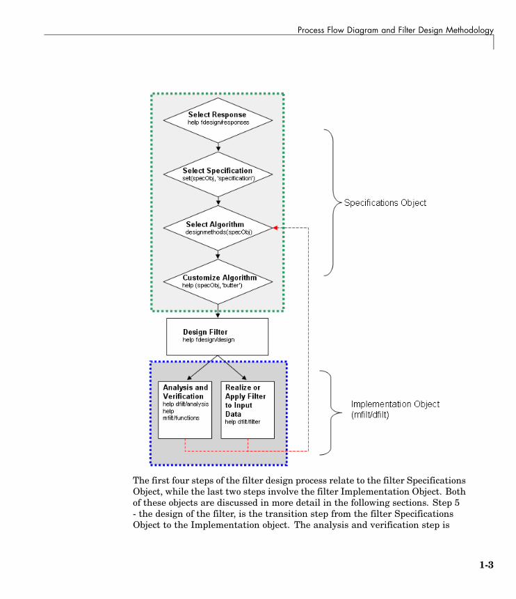
Exploring the Process Flow DiagramThe process flow diagram shown in the following figure lists the steps andshows the order of the filter design process.
1-2
Process Flow Diagram and Filter Design Methodology
The first four steps of the filter design process relate to the filter SpecificationsObject, while the last two steps involve the filter Implementation Object. Bothof these objects are discussed in more detail in the following sections. Step 5- the design of the filter, is the transition step from the filter SpecificationsObject to the Implementation object. The analysis and verification step is
1-3

1 Designing a Filter — Process Overview
completely optional. It provides methods for the filter designer to ensure thatthe filter complies with all design criteria. Depending on the results of thisverification, you can loop back to steps 3 and 4, to either choose a differentalgorithm, or to customize the current one. You may also wish to go back tosteps 3 or 4 after you filter the input data with the designed filter (step 7),and find that you wish to tweak the filter or change it further.
The diagram shows the help command for each step. Enter the help lineat the MATLAB® command prompt to receive instructions and furtherdocumentation links for the particular step. Not all of the steps have to beexecuted explicitly. For example, you could go from step 1 directly to step 5,and the interim three steps are done for you by Filter Design Toolbox.
The following are the details for each of the steps shown above.
Selecting a ResponseIf you type:
help fdesign/responses
at the MATLAB command prompt, you see a complete list of all possible filterresponses available in Filter Design Toolbox. After you choose a response,say bandpass, you start the design of the Specifications Object by typing thefollowing:
d = fdesign.bandpass
This step cannot be skipped, nor is it automatically completed for you by FilterDesign Toolbox. You must select a response to initiate the filter design process.
Selecting a SpecificationA specification is an array of design parameters for a given filter. Thespecification itself is a property of the Specifications Object.
Note A specification is not the same as the Specifications Object, rather aSpecifications Object contains a specification as one of its properties.
1-4

Process Flow Diagram and Filter Design Methodology
When you select a filter response, there is a number of different specificationsavailable, each containing a different combination of design parameters.In the following example, first set the filter response, then ask for thespecifications listing.
>> d = fdesign.bandpass; % step 1 - choose the response>> set (d, 'specification')
ans =
'Fst1,Fp1,Fp2,Fst2,Ast1,Ap,Ast2''N,F3dB1,F3dB2''N,F3dB1,F3dB2,Ap''N,F3dB1,F3dB2,Ast''N,F3dB1,F3dB2,Ast1,Ap,Ast2''N,F3dB1,F3dB2,BWp''N,F3dB1,F3dB2,BWst''N,Fc1,Fc2''N,Fp1,Fp2,Ap''N,Fp1,Fp2,Ast1,Ap,Ast2''N,Fst1,Fp1,Fp2,Fst2''N,Fst1,Fp1,Fp2,Fst2,Ap''N,Fst1,Fst2,Ast''Nb,Na,Fst1,Fp1,Fp2,Fst2'
>> d = fdesign.decimator; % step 1 - choose the response<<% get a list of available specifications>> set (d, 'specification')ans =
'TW,Ast''N''N,Ast''N,TW'
After you select the specification that includes all of the given filter’s designparameters, you can set it as follows:
>> d = fdesign.lowpass; % step 1>> % step 2: get a list of available specifications>> set (d, 'specification')
1-5

1 Designing a Filter — Process Overview
ans =
'Fp,Fst,Ap,Ast''N,F3dB''N,F3dB,Ap''N,F3dB,Ap,Ast''N,F3dB,Ast''N,F3dB,Fst''N,Fc''N,Fc,Ap,Ast''N,Fp,Ap''N,Fp,Ap,Ast''N,Fp,F3dB''N,Fp,Fst''N,Fp,Fst,Ap''N,Fp,Fst,Ast''N,Fst,Ap,Ast''N,Fst,Ast''Nb,Na,Fp,Fst'
>> %step 2: set the required specification>> set (d, 'specification', 'N,Fc')
If you do not perform this step explicitly, Filter Design Toolbox selects adefault specification for the response you chose in , and even provides defaultvalues for all design parameters included in the specification.
Selecting an AlgorithmThe availability of algorithms depends on both the chosen filter responseand the design parameters. In other words, for the same lowpass filter,changing the specification string also changes the available algorithms. Inthe following example, for a lowpass filter and a specification of 'N, Fc',only one algorithm is available—window. However, for a specification of'Fp,Fst,Ap,Ast', a number of algorithms is available.
>> %step 2: set the required specification>> set (d, 'specification', 'N,Fc')>> designmethods (d) %step3: get available algorithms
1-6

Process Flow Diagram and Filter Design Methodology
Design Methods for class fdesign.lowpass (N,Fc):
window
>> %step2: set a different specification>> set (d, 'specification', 'Fp,Fst,Ap,Ast')>> designmethods (d) %step3: get available algorithms
Design Methods for class fdesign.lowpass (Fp,Fst,Ap,Ast):
buttercheby1cheby2ellipequirippleifirkaiserwinmultistage
To apply the chosen algorithm, (the Butterworth algorithm in this example),evaluate the following:
>> f = design(d, 'butter');
The preceding code actually creates the filter, where f is the filterImplementation Object. This concept is discussed further in the next step.
If you do not perform this step explicitly, Filter Design Toolbox automaticallyselects the optimum algorithm for the chosen response and specification.
Customizing the AlgorithmThe customization options available for any given algorithm depend not onlyon the algorithm itself, selected in , but also on the specification selectedin . To explore all the available options, type the following at the MATLABcommand prompt:
1-7

1 Designing a Filter — Process Overview
help (d, 'algorithm-name')
where d is the Specifications Object, and algorithm-name is the name of thealgorithm in quotes, such as 'butter' or 'cheby1'.
The application of these customization options takes place during the ,because these options are the properties of the filter Implementation Object,not the Specification Object.
If you do not perform this step explicitly, Filter Design Toolbox automaticallyselects the optimal algorithm structure as well as other options.
Designing the FilterThis next task introduces a new object, the Filter Object, or dfilt. To create afilter, use the design command:
>> % design filter w/o specifying the algorithm>> f = design(d);
where f is the Filter Object also referred to sometimes as dfilt, and d isthe Specifications Object. This code creates a filter without specifying thealgorithm. When the algorithm is not specified, Filter Design Toolbox selectsthe best available one.
To apply the algorithm chosen in , use the same design command, but specifythe Butterworth algorithm as follows:
>> f = design(d, 'butter');
where f is the new Filter Object, and d is the Specifications Object.
To obtain help and see all the available options, type:
>> help fdesign/design
This help command describes not only the options for the design commanditself, but also options that pertain to the method or the algorithm. If youare customizing the algorithm, you apply these options in this step. In thefollowing example, you design a bandpass filter, and then modify the filterstructure:
1-8

Process Flow Diagram and Filter Design Methodology
>> f = design(d, 'butter', 'filterstructure', 'df2sos')
f =
FilterStructure: 'Direct-Form II, Second-Order Sections'Arithmetic: 'double'sosMatrix: [7x6 double]
ScaleValues: [8x1 double]PersistentMemory: false
The filter design step, just like the first task of choosing a response, must beperformed explicitly. Filter Design Toolbox does not create a filter unlessyou specifically tell it to do so.
Design AnalysisAfter the filter is designed you may wish to analyze it to determine if the filtersatisfies the design criteria. In Filter Design Toolbox, analysis is broken intothree main sections:
• Frequency domain analysis — Includes magnitude response, group delay,and poll zero
• Time domain analysis — Includes impulse and step response
• Implementation analysis — Includes quantization noise and cost
To display help for analysis of a discrete-time filter, type:
>> help dfilt/analysis
To display help for analysis of a multirate filter, type:
>> help mfilt/functions
To display help for analysis of a farrow filter, type:
>> help farrow/functions
To analyze your filter, you must explicitly perform this step.
1-9

1 Designing a Filter — Process Overview
Realize or Apply the Filter to Input DataAfter the filter is designed and optimized, it can be used to filter actual inputdata. The basic filter command takes input data x, filters it through the FilterObject, and produces output y:
>> y = filter (FilterObj, x)
This step is never automatically performed for you by Filter Design Toolbox.To filter your data, you must explicitly execute this step. To understand howthe filtering commands work, type:
>> help dfilt/filter
Note If you have Simulink®, you have the option of exporting this filterto a Simulink block using the realizemdl command. To get help on thiscommand, type:
>> help realizemdl
1-10

2
Using the Filterbuilder GUI
The Graphical Interface to Fdesign(p. 2-2)
filterbuilder GUI
Designing a FIR Filter Usingfilterbuilder (p. 2-11)
FIR filter design example

2 Using the Filterbuilder GUI
The Graphical Interface to Fdesign
In this section...
“Introduction to Filterbuilder” on page 2-2
“Filterbuilder Design Process” on page 2-3
“Select a Response” on page 2-3
“Select a Specification” on page 2-6
“Select an Algorithm” on page 2-6
“Customize the Algorithm” on page 2-7
“Analyze the Design” on page 2-9
“Realize or Apply the Filter to Input Data” on page 2-9
Introduction to FilterbuilderThe filterbuilder function provides a graphical interface to the fdesignobject-object oriented filter design paradigm and is intended to reducedevelopment time during the filter design process. filterbuilder uses aspecification-centered approach to find the best algorithm for the desiredresponse.
The filterbuilder GUI contains many features that are not available inFDATool. For instance:
• Mulitrate/multistage FIR filters for efficient narrow-transition banddesigns
• Automatically generated optimal multistage interpolators and decimators
• Optimal multistage Nyquist filters
• IIR halfband designs (including IIR filters with approximately linear phase)
• CIC designs (including CIC compensators)
• Farrow filter designs
• Wave digital filter designs
• Arbitrary magnitude and phase designs
2-2

The Graphical Interface to Fdesign
Filterbuilder Design ProcessThe design process when using filterbuilder is similar to the processoutlined in the section titledChapter 1, “Designing a Filter — ProcessOverview” in the Getting Started guide. The idea is to choose the constraintsand specifications of the filter, and to use those as a starting point in thedesign. Postponing the choice of algorithm for the filter allows the best designmethod to be determined automatically, based upon the desired performancecriteria. The following are the details of each of the steps for designing afilter with filterbuilder.
Select a ResponseWhen you open the filterbuilder tool by typing:
filterbuilder
at the MATLAB command prompt, the Response Selection dialog boxappears, listing all possible filter responses available in Filter Design Toolbox:
Note This step cannot be skipped because it is not automatically completedfor you by Filter Design Toolbox. You must select a response to initiate thefilter design process.
2-3

2 Using the Filterbuilder GUI
After you choose a response, say bandpass, you start the design of theSpecifications Object, and the Bandpass Design dialog box appears.This dialog box contains a Main pane, a Data Types pane and a CodeGeneration pane. The specifications of your filter are generally set in theMain pane of the dialog box.
The Data Types pane provides settings for precision and data types, and theCode Generation pane contains options for various implementations of thecompleted filter design. More information about the Data Types and CodeGeneration panes can be found in the section titled “Filterbuilder DialogBox” in the Filter Design Toolbox Reference Guide.
For the initial design of your filter, you will mostly use the Main pane.
2-4

The Graphical Interface to Fdesign
The Bandpass Design dialog box contains all the parameters you need todetermine the specifications of a bandpass filter. The parameters listed inthe Main pane depend upon the type of filter you are designing. However,no matter what type of filter you have chosen in the Response Selectiondialog box, the filter design dialog box contains the Main, Data Types, andCode Generation panes.
2-5
2 Using the Filterbuilder GUI
Select a SpecificationTo choose the specification for the bandpass filter, you can begin by selectingan Impulse Response, Order Mode, and Filter Type in the FilterSpecifications frame of the Main Pane. You can further specify theresponse of your filter by setting frequency and magnitude specifications inthe appropriate frames on the Main Pane.
Note Frequency, Magnitude, and Algorithm specifications areinterdependent and may change based upon your Filter Specificationsselections. When choosing specifications for your filter, select your FilterSpecifications first and work your way down the dialog box- this approachensures that the best settings for dependent specifications display as availablein the dialog box.
Select an AlgorithmThe algorithms available for your filter depend upon the filter response anddesign parameters you have selected in the previous steps. For example, in thecase of a bandpass filter, if the impulse response selected is IIR and the OrderMode field is set toMinimum, the design methods available is Butterworth,Chebyshev type I or II, or Elliptic, whereas if the Order Mode field is setto Specify, the design method available is IIR least p-norm.
2-6

The Graphical Interface to Fdesign
Customize the AlgorithmBy expanding the Design options section of the Algorithm frame, youcan further customize the algorithm specified. The options available willdepend upon the algorithm and settings that have already been selected inthe dialog box. In the case of a bandpass IIR filter using the Butterworth
2-7

2 Using the Filterbuilder GUI
method, design options such as Match Exactly are available, as shown inthe following figure.
2-8

The Graphical Interface to Fdesign
Analyze the DesignTo analyze the filter response, click on the View Filter Response button. TheFilter Visualization Tool opens displaying the magnitude plot of the filterresponse.
Realize or Apply the Filter to Input DataWhen you have achieved the desired filter response through design iterationsand analysis using the Filter Visualization Tool, apply the filter to theinput data. Again, this step is never automatically performed for you by FilterDesign Toolbox. To filter your data, you must explicitly execute this step. Inthe Filter Visualization Tool, click OK and Filter Design Toolbox createsthe filter object with the name specified in the Save variable as field andexports it to the MATLAB workspace.
The filter is then ready to be used to filter actual input data. The basic filtercommand takes input data x, filters it through the Filter Object, and producesoutput y:
>> y = filter (FilterObj, x)
To understand how the filtering commands work, type:
>> help dfilt/filter
2-9

2 Using the Filterbuilder GUI
Tip If you have Simulink, you have the option of exporting this filter toa Simulink block using the realizemdl command. To get help on thiscommand, type:
>> help realizemdl
2-10

Designing a FIR Filter Using filterbuilder
Designing a FIR Filter Using filterbuilder
FIR Filter Design
Example – Using Filterbuilder to Design a Finite Impulse Response(FIR) FilterTo design a lowpass FIR filter using filterbuilder:
1 Open the Filterbuilder GUI by typing the following at the MATLAB prompt:
filterbuilder
The Response Selection dialog box appears. In this dialog box, you canselect from a list of filter response types. Select Lowpass in the list box.
2 Hit the OK button. The Lowpass Design dialog box opens. Here youcan specify the writable parameters of the the Lowpass filter object. Thecomponents of the Main frame of this dialog box are described in thesection titled “Lowpass Filter Design Dialog Box — Main Pane”. In thedialog box, make the following changes:
• Enter a Fpass value of 0.55.
• Enter a Fstop value of 0.65.
2-11

2 Using the Filterbuilder GUI
3 Click Apply, and the following message appears at the MATLAB prompt:
The variable 'Hlp' has been exported to the command window.
2-12
Designing a FIR Filter Using filterbuilder
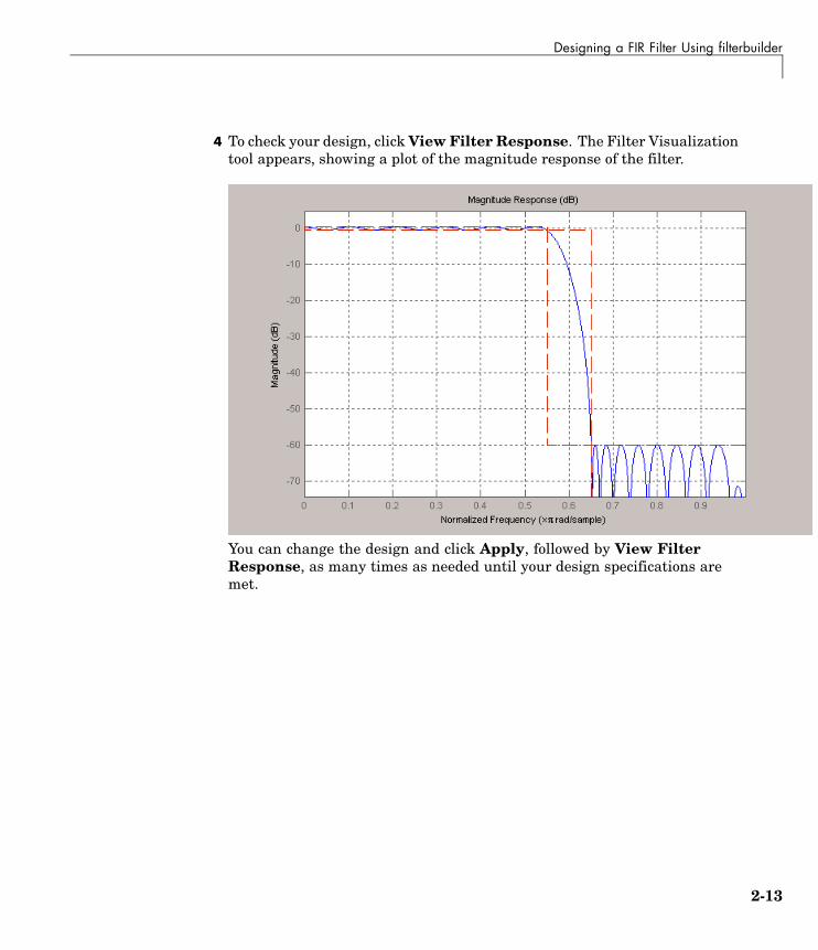
4 To check your design, click View Filter Response. The Filter Visualizationtool appears, showing a plot of the magnitude response of the filter.
You can change the design and click Apply, followed by View FilterResponse, as many times as needed until your design specifications aremet.
2-13

2 Using the Filterbuilder GUI
2-14

3
Digital FrequencyTransformations
Details and Methodology (p. 3-2) Presents and defines the problemof using digital frequencytransformation
Frequency Transformations for RealFilters (p. 3-11)
Discusses the functions fortransforming real filters to otherreal filters
Frequency Transformations forComplex Filters (p. 3-26)
Describes the functions fortransforming complex filters to othercomplex filters, or real filters tocomplex filters

3 Digital Frequency Transformations
Details and Methodology
In this section...
“Overview of Transformations” on page 3-2
“Selecting Features Subject to Transformation” on page 3-6
“Mapping from Prototype Filter to Target Filter” on page 3-8
“Summary of Frequency Transformations” on page 3-10
Overview of TransformationsConverting existing FIR or IIR filter designs to a modified IIR form is oftendone using allpass frequency transformations. Although the resulting designscan be considerably more expensive in terms of dimensionality than theprototype (original) filter, their ease of use in fixed or variable applications isa big advantage.
The general idea of the frequency transformation is to take an existingprototype filter and produce another filter from it that retains some of thecharacteristics of the prototype, in the frequency domain. Transformationfunctions achieve this by replacing each delaying element of the prototypefilter with an allpass filter carefully designed to have a prescribed phasecharacteristic for achieving the modifications requested by the designer.
The basic form of mapping commonly used is
The HA(z) is an Nth-order allpass mapping filter given by
3-2

Details and Methodology
where
Ho(z) — Transfer function of the prototype filter
HA(z) — Transfer function of the allpass mapping filter
HT(z) — Transfer function of the target filter
Let’s look at a simple example of the transformation given by
The target filter has its poles and zeroes flipped across the origin of the realand imaginary axes. For the real filter prototype, it gives a mirror effectagainst 0.5, which means that lowpass Ho(z) gives rise to a real highpassHT(z). This is shown in the following figure for the prototype filter designedas a third-order halfband elliptic filter.
3-3

3 Digital Frequency Transformations
0 0.2 0.4 0.6 0.8 1−60
−50
−40
−30
−20
−10
0Prototype filter
|H(ω
)| in
dB
Normalized Frequency (×π rad/sample)0 0.2 0.4 0.6 0.8 1
−60
−50
−40
−30
−20
−10
0Target filter
|H(ω
)| in
dB
Normalized Frequency (×π rad/sample)
Prototype filter Pole−Zero plot Target filter Pole−Zero plot
Example of a Simple Mirror Transformation
The choice of an allpass filter to provide the frequency mapping is necessaryto provide the frequency translation of the prototype filter frequency responseto the target filter by changing the frequency position of the features from theprototype filter without affecting the overall shape of the filter response.
The phase response of the mapping filter normalized to π can be interpretedas a translation function:
The graphical interpretation of the frequency transformation is shown in thefigure below. The complex multiband transformation takes a real lowpassfilter and converts it into a number of passbands around the unit circle.
3-4

Details and Methodology
Graphical Interpretation of the Mapping Process
Most of the frequency transformations are based on the second-order allpassmapping filter:
The two degrees of freedom provided by α1 and α2 choices are not fully usedby the usual restrictive set of “flat-top” classical mappings like lowpass tobandpass. Instead, any two transfer function features can be migrated to(almost) any two other frequency locations if α1 and α2 are chosen so as to keepthe poles of HA(z) strictly outside the unit circle (since HA(z) is substitutedfor z in the prototype transfer function). Moreover, as first pointed outby Constantinides, the selection of the outside sign influences whether theoriginal feature at zero can be moved (the minus sign, a condition known
3-5

3 Digital Frequency Transformations
as “DC mobility”) or whether the Nyquist frequency can be migrated (the“Nyquist mobility” case arising when the leading sign is positive).
All the transformations forming the package are explained in the nextsections of the tutorial. They are separated into those operating on realfilters and those generating or working with complex filters. The choice oftransformation ranges from standard Constantinides first and second-orderones [1][2] up to the real multiband filter by Mullis and Franchitti [3], andthe complex multiband filter and real/complex multipoint ones by Krukowski,Cain and Kale [4].
Selecting Features Subject to TransformationChoosing the appropriate frequency transformation for achieving the requiredeffect and the correct features of the prototype filter is very importantand needs careful consideration. It is not advisable to use a first-ordertransformation for controlling more than one feature. The mapping filterwill not give enough flexibility. It is also not good to use higher ordertransformation just to change the cutoff frequency of the lowpass filter. Theincrease of the filter order would be too big, without considering the additionalreplica of the prototype filter that may be created in undesired places.
Feature Selection for Real Lowpass to Bandpass Transformation
3-6
Details and Methodology
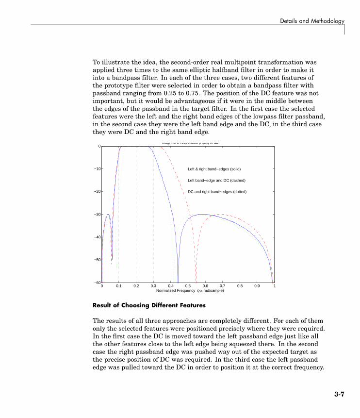
To illustrate the idea, the second-order real multipoint transformation wasapplied three times to the same elliptic halfband filter in order to make itinto a bandpass filter. In each of the three cases, two different features ofthe prototype filter were selected in order to obtain a bandpass filter withpassband ranging from 0.25 to 0.75. The position of the DC feature was notimportant, but it would be advantageous if it were in the middle betweenthe edges of the passband in the target filter. In the first case the selectedfeatures were the left and the right band edges of the lowpass filter passband,in the second case they were the left band edge and the DC, in the third casethey were DC and the right band edge.
0 0.1 0.2 0.3 0.4 0.5 0.6 0.7 0.8 0.9 1−60
−50
−40
−30
−20
−10
0
Left & right band−edges (solid)
Left band−edge and DC (dashed)
DC and right band−edges (dotted)
Magniture responses |H(ω)| in dB
Normalized Frequency (×π rad/sample)
Result of Choosing Different Features
The results of all three approaches are completely different. For each of themonly the selected features were positioned precisely where they were required.In the first case the DC is moved toward the left passband edge just like allthe other features close to the left edge being squeezed there. In the secondcase the right passband edge was pushed way out of the expected target asthe precise position of DC was required. In the third case the left passbandedge was pulled toward the DC in order to position it at the correct frequency.
3-7

3 Digital Frequency Transformations
The conclusion is that if only the DC can be anywhere in the passband, theedges of the passband should have been selected for the transformation. Formost of the cases requiring the positioning of passbands and stopbands,designers should always choose the position of the edges of the prototypefilter in order to make sure that they get the edges of the target filter in thecorrect places. Frequency responses for the three cases considered are shownin the figure. The prototype filter was a third-order elliptic lowpass filterwith cutoff frequency at 0.5.
The MATLAB code used to generate the figure is given here.
The prototype filter is a halfband elliptic, real, third-order lowpass filter:
[b, a] = ellip(3, 0.1, 30, 0.409);
In the example the requirements are set to create a real bandpass filterwith passband edges at 0.1 and 0.3 out of the real lowpass filter having thecutoff frequency at 0.5. This is attempted in three different ways. In the firstapproach both edges of the passband are selected, in the second approach theleft edge of the passband and the DC are chosen, while in the third approachthe DC and the right edge of the passband are taken:
[num1,den1] = iirlp2xn(b, a, [-0.5, 0.5], [0.1, 0.3]);[num2,den2] = iirlp2xn(b, a, [-0.5, 0.0], [0.1, 0.2]);[num3,den3] = iirlp2xn(b, a, [ 0.0, 0.5], [0.2, 0.3]);
Mapping from Prototype Filter to Target FilterIn general the frequency mapping converts the prototype filter, Ho(z), to thetarget filter, HT(z), using the NAth-order allpass filter, HA(z). The generalform of the allpass mapping filter is given in . The frequency mapping is amathematical operation that replaces each delayer of the prototype filterwith an allpass filter. There are two ways of performing such mapping. Thechoice of the approach is dependent on how prototype and target filters arerepresented.
When the Nth-order prototype filter is given with pole-zero form
3-8

Details and Methodology
the mapping will replace each pole, pi, and each zero, zi, with a number ofpoles and zeros equal to the order of the allpass mapping filter:
The root finding needs to be used on the bracketed expressions in order to findthe poles and zeros of the target filter.
When the prototype filter is described in the numerator-denominator form:
Then the mapping process will require a number of convolutions in order tocalculate the numerator and denominator of the target filter:
For each coefficient αi and βi of the prototype filter the NAth-order polynomialsmust be convolved N times. Such approach may cause rounding errors for largeprototype filters and/or high order mapping filters. In such a case the usershould consider the alternative of doing the mapping using via poles and zeros.
3-9

3 Digital Frequency Transformations
Summary of Frequency Transformations
Advantages
• Most frequency transformations are described by closed-form solutions orcan be calculated from the set of linear equations.
• They give predictable and familiar results.
• Ripple heights from the prototype filter are preserved in the target filter.
• They are architecturally appealing for variable and adaptive filters.
Disadvantages
• There are cases when using optimization methods to design the requiredfilter gives better results.
• High-order transformations increase the dimensionality of the target filter,which may give expensive final results.
• Starting from fresh designs helps avoid locked-in compromises.
3-10

Frequency Transformations for Real Filters
Frequency Transformations for Real Filters
In this section...
“Overview” on page 3-11
“Real Frequency Shift” on page 3-11
“Real Lowpass to Real Lowpass” on page 3-13
“Real Lowpass to Real Highpass” on page 3-15
“Real Lowpass to Real Bandpass” on page 3-17
“Real Lowpass to Real Bandstop” on page 3-19
“Real Lowpass to Real Multiband” on page 3-21
“Real Lowpass to Real Multipoint” on page 3-23
OverviewThis section discusses real frequency transformations that take the reallowpass prototype filter and convert it into a different real target filter. Thetarget filter has its frequency response modified in respect to the frequencyresponse of the prototype filter according to the characteristic of the appliedfrequency transformation.
Real Frequency ShiftReal frequency shift transformation uses a second-order allpass mappingfilter. It performs an exact mapping of one selected feature of the frequencyresponse into its new location, additionally moving both the Nyquist and DCfeatures. This effectively moves the whole response of the lowpass filter bythe distance specified by the selection of the feature from the prototype filterand the target filter. As a real transformation, it works in a similar way forpositive and negative frequencies.
with α given by
3-11

3 Digital Frequency Transformations
where
ωold — Frequency location of the selected feature in the prototype filter
ωnew — Position of the feature originally at ωold in the target filter
The following example shows how this transformation can be used to movethe response of the prototype lowpass filter in either direction. Please notethat because the target filter must also be real, the response of the targetfilter will inherently be disturbed at frequencies close to Nyquist and close toDC. Here is the MATLAB code for generating the example in the figure.
The prototype filter is a halfband elliptic, real, third-order lowpass filter:
[b, a] = ellip(3, 0.1, 30, 0.409);
The example transformation moves the feature originally at 0.5 to 0.9:
[num,den] = iirshift(b, a, 0.5, 0.9);
3-12

Frequency Transformations for Real Filters
0 0.1 0.2 0.3 0.4 0.5 0.6 0.7 0.8 0.9 1−60
−50
−40
−30
−20
−10
0Prototype filter
|H(ω
)|in
dB
Normalized Frequency (×π rad/sample)
ωo
0 0.1 0.2 0.3 0.4 0.5 0.6 0.7 0.8 0.9 1−60
−50
−40
−30
−20
−10
0Target filter
|H(ω
)| in
dB
Normalized Frequency (×π rad/sample)
ωt
Example of Real Frequency Shift Mapping
Real Lowpass to Real LowpassReal lowpass filter to real lowpass filter transformation uses a first-orderallpass mapping filter. It performs an exact mapping of one feature of thefrequency response into the new location keeping DC and Nyquist featuresfixed. As a real transformation, it works in a similar way for positive andnegative frequencies. It is important to mention that using first-ordermapping ensures that the order of the filter after the transformation is thesame as it was originally.
with α given by
3-13

3 Digital Frequency Transformations
where
ωold — Frequency location of the selected feature in the prototype filter
ωnew — Frequency location of the same feature in the target filter
The example below shows how to modify the cutoff frequency of the prototypefilter. The MATLAB code for this example is shown in the following figure.
The prototype filter is a halfband elliptic, real, third-order filter:
[b, a] = ellip(3, 0.1, 30, 0.409);
The cutoff frequency moves from 0.5 to 0.75:
[num,den] = iirlp2lp(b, a, 0.5, 0.75);
3-14

Frequency Transformations for Real Filters
0 0.1 0.2 0.3 0.4 0.5 0.6 0.7 0.8 0.9 1−60
−50
−40
−30
−20
−10
0Prototype filter
|H(ω
)|in
dB
Normalized Frequency (×π rad/sample)
ωo
0 0.1 0.2 0.3 0.4 0.5 0.6 0.7 0.8 0.9 1−60
−50
−40
−30
−20
−10
0Target filter
|H(ω
)| in
dB
Normalized Frequency (×π rad/sample)
ωt
Example of Real Lowpass to Real Lowpass Mapping
Real Lowpass to Real HighpassReal lowpass filter to real highpass filter transformation uses a first-orderallpass mapping filter. It performs an exact mapping of one feature of thefrequency response into the new location additionally swapping DC andNyquist features. As a real transformation, it works in a similar way forpositive and negative frequencies. Just like in the previous transformationbecause of using a first-order mapping, the order of the filter before and afterthe transformation is the same.
with α given by
3-15

3 Digital Frequency Transformations
where
ωold — Frequency location of the selected feature in the prototype filter
ωnew — Frequency location of the same feature in the target filter
The example below shows how to convert the lowpass filter into a highpassfilter with arbitrarily chosen cutoff frequency. In the MATLAB code below,the lowpass filter is converted into a highpass with cutoff frequency shiftedfrom 0.5 to 0.75. Results are shown in the figure.
The prototype filter is a halfband elliptic, real, third-order filter:
[b, a] = ellip(3, 0.1, 30, 0.409);
The example moves the cutoff frequency from 0.5 to 0.75:
[num,den] = iirlp2lp(b, a, 0.5, 0.75);
3-16

Frequency Transformations for Real Filters
0 0.1 0.2 0.3 0.4 0.5 0.6 0.7 0.8 0.9 1−60
−50
−40
−30
−20
−10
0Prototype filter
|H(ω
)|in
dB
Normalized Frequency (×π rad/sample)
ωo
0 0.1 0.2 0.3 0.4 0.5 0.6 0.7 0.8 0.9 1−60
−50
−40
−30
−20
−10
0Target filter
|H(ω
)| in
dB
Normalized Frequency (×π rad/sample)
ωt
Example of Real Lowpass to Real Highpass Mapping
Real Lowpass to Real BandpassReal lowpass filter to real bandpass filter transformation uses a second-orderallpass mapping filter. It performs an exact mapping of two features of thefrequency response into their new location additionally moving a DC featureand keeping the Nyquist feature fixed. As a real transformation, it works in asimilar way for positive and negative frequencies.
with α and β given by
3-17

3 Digital Frequency Transformations
where
ωold — Frequency location of the selected feature in the prototype filter
ωnew,1 — Position of the feature originally at (-ωold) in the target filter
ωnew,2 — Position of the feature originally at (+ωold) in the target filter
The example below shows how to move the response of the prototype lowpassfilter in either direction. Please note that because the target filter mustalso be real, the response of the target filter will inherently be disturbed atfrequencies close to Nyquist and close to DC. Here is the MATLAB code forgenerating the example in the figure.
The prototype filter is a halfband elliptic, real, third-order lowpass filter:
[b, a] = ellip(3, 0.1, 30, 0.409);
The example transformation creates the passband between 0.5 and 0.75:
[num,den] = iirlp2bp(b, a, 0.5, [0.5, 0.75]);
3-18

Frequency Transformations for Real Filters
0 0.1 0.2 0.3 0.4 0.5 0.6 0.7 0.8 0.9 1−60
−50
−40
−30
−20
−10
0Prototype filter
|H(ω
)|in
dB
Normalized Frequency (×π rad/sample)
ωo
0 0.1 0.2 0.3 0.4 0.5 0.6 0.7 0.8 0.9 1−60
−50
−40
−30
−20
−10
0Target filter
|H(ω
)| in
dB
Normalized Frequency (×π rad/sample)
ωt1 ωt2
Example of Real Lowpass to Real Bandpass Mapping
Real Lowpass to Real BandstopReal lowpass filter to real bandstop filter transformation uses a second-orderallpass mapping filter. It performs an exact mapping of two features of thefrequency response into their new location additionally moving a Nyquistfeature and keeping the DC feature fixed. This effectively creates a stopbandbetween the selected frequency locations in the target filter. As a realtransformation, it works in a similar way for positive and negative frequencies.
with α and β given by
3-19

3 Digital Frequency Transformations
where
ωold — Frequency location of the selected feature in the prototype filter
ωnew,1 — Position of the feature originally at (-ωold) in the target filter
ωnew,2 — Position of the feature originally at (+ωold) in the target filter
The following example shows how this transformation can be used to convertthe prototype lowpass filter with cutoff frequency at 0.5 into a real bandstopfilter with the same passband and stopband ripple structure and stopbandpositioned between 0.5 and 0.75. Here is the MATLAB code for generating theexample in the figure.
The prototype filter is a halfband elliptic, real, third-order lowpass filter:
[b, a] = ellip(3, 0.1, 30, 0.409);
The example transformation creates a stopband from 0.5 to 0.75:
[num,den] = iirlp2bs(b, a, 0.5, [0.5, 0.75]);
3-20

Frequency Transformations for Real Filters
0 0.1 0.2 0.3 0.4 0.5 0.6 0.7 0.8 0.9 1−60
−50
−40
−30
−20
−10
0Prototype filter
|H(ω
)|in
dB
Normalized Frequency (×π rad/sample)
ωo
0 0.1 0.2 0.3 0.4 0.5 0.6 0.7 0.8 0.9 1−60
−50
−40
−30
−20
−10
0Target filter
|H(ω
)| in
dB
Normalized Frequency (×π rad/sample)
ωt1 ωt2
Example of Real Lowpass to Real Bandstop Mapping
Real Lowpass to Real MultibandThis high-order transformation performs an exact mapping of one selectedfeature of the prototype filter frequency response into a number of newlocations in the target filter. Its most common use is to convert a real lowpasswith predefined passband and stopband ripples into a real multiband filterwith N arbitrary band edges, where N is the order of the allpass mapping filter.
The coefficients α are given by
3-21

3 Digital Frequency Transformations
where
ωold,k — Frequency location of the first feature in the prototype filter
ωnew,k — Position of the feature originally at ωold,k in the target filter
The mobility factor, S, specifies the mobility or either DC or Nyquist feature:
The example below shows how this transformation can be used to convert theprototype lowpass filter with cutoff frequency at 0.5 into a filter having anumber of bands positioned at arbitrary edge frequencies 1/5, 2/5, 3/5 and 4/5.Parameter S was such that there is a passband at DC. Here is the MATLABcode for generating the figure.
The prototype filter is a halfband elliptic, real, third-order lowpass filter:
[b, a] = ellip(3, 0.1, 30, 0.409);
The example transformation creates three passbands, from DC to 0.2, from0.4 to 0.6 and from 0.8 to Nyquist:
[num,den] = iirlp2mb(b, a, 0.5, [0.2, 0.4, 0.6, 0.8], `pass');
3-22

Frequency Transformations for Real Filters
0 0.1 0.2 0.3 0.4 0.5 0.6 0.7 0.8 0.9 1−60
−50
−40
−30
−20
−10
0Prototype filter
|H(ω
)|in
dB
Normalized Frequency (×π rad/sample)
ωo
0 0.1 0.2 0.3 0.4 0.5 0.6 0.7 0.8 0.9 1−60
−50
−40
−30
−20
−10
0Target filter
|H(ω
)| in
dB
Normalized Frequency (×π rad/sample)
ωt1 ωt2 ωt3 ωt4
Example of Real Lowpass to Real Multiband Mapping
Real Lowpass to Real MultipointThis high-order frequency transformation performs an exact mapping of anumber of selected features of the prototype filter frequency response to theirnew locations in the target filter. The mapping filter is given by the generalIIR polynomial form of the transfer function as given below.
For the Nth-order multipoint frequency transformation the coefficients α are
3-23

3 Digital Frequency Transformations
where
ωold,k — Frequency location of the first feature in the prototype filter
ωnew,k — Position of the feature originally at ωold,k in the target filter
The mobility factor, S, specifies the mobility of either DC or Nyquist feature:
The example below shows how this transformation can be used to movefeatures of the prototype lowpass filter originally at -0.5 and 0.5 to their newlocations at 0.5 and 0.75, effectively changing a position of the filter passband.Here is the MATLAB code for generating the figure.
The prototype filter is a halfband elliptic, real, third-order lowpass filter:
[b, a] = ellip(3, 0.1, 30, 0.409);
The example transformation creates a passband from 0.5 to 0.75:
[num,den] = iirlp2xn(b, a, [-0.5, 0.5], [0.5, 0.75], `pass');
3-24

Frequency Transformations for Real Filters
0 0.1 0.2 0.3 0.4 0.5 0.6 0.7 0.8 0.9 1−60
−50
−40
−30
−20
−10
0Prototype filter
|H(ω
)|in
dB
Normalized Frequency (×π rad/sample)
ωo2
0 0.1 0.2 0.3 0.4 0.5 0.6 0.7 0.8 0.9 1−60
−50
−40
−30
−20
−10
0Target filter
|H(ω
)| in
dB
Normalized Frequency (×π rad/sample)
ωt1 ωt2
Example of Real Lowpass to Real Multipoint Mapping
3-25
3 Digital Frequency Transformations
Frequency Transformations for Complex Filters
In this section...
“Overview” on page 3-26
“Complex Frequency Shift” on page 3-26
“Real Lowpass to Complex Bandpass” on page 3-28
“Real Lowpass to Complex Bandstop” on page 3-30
“Real Lowpass to Complex Multiband” on page 3-32
“Real Lowpass to Complex Multipoint” on page 3-34
“Complex Bandpass to Complex Bandpass” on page 3-36
OverviewThis section discusses complex frequency transformation that take thecomplex prototype filter and convert it into a different complex targetfilter. The target filter has its frequency response modified in respect to thefrequency response of the prototype filter according to the characteristic of theapplied frequency transformation from:
Complex Frequency ShiftComplex frequency shift transformation is the simplest first-ordertransformation that performs an exact mapping of one selected feature of thefrequency response into its new location. At the same time it rotates thewhole response of the prototype lowpass filter by the distance specified by theselection of the feature from the prototype filter and the target filter.
with α given by
where
3-26

Frequency Transformations for Complex Filters
ωold — Frequency location of the selected feature in the prototype filter
ωnew — Position of the feature originally at ωold in the target filter
A special case of the complex frequency shift is a, so called, HilbertTransformer. It can be designed by setting the parameter to |α|=1, that is
The example below shows how to apply this transformation to rotate theresponse of the prototype lowpass filter in either direction. Please note thatbecause the transformation can be achieved by a simple phase shift operator,all features of the prototype filter will be moved by the same amount. Here isthe MATLAB code for generating the example in the figure.
The prototype filter is a halfband elliptic, real, third-order lowpass filter:
[b, a] = ellip(3, 0.1, 30, 0.409);
The example transformation moves the feature originally at 0.5 to 0.9:
[num,den] = iirshift(b, a, 0.5, 0.9);
3-27

3 Digital Frequency Transformations
−1 −0.8 −0.6 −0.4 −0.2 0 0.2 0.4 0.6 0.8 1−60
−50
−40
−30
−20
−10
0Prototype filter
|H(ω
)|in
dB
Normalized Frequency (×π rad/sample)
ωo
−1 −0.8 −0.6 −0.4 −0.2 0 0.2 0.4 0.6 0.8 1−60
−50
−40
−30
−20
−10
0Target filter
|H(ω
)| in
dB
Normalized Frequency (×π rad/sample)
ωt
Example of Complex Frequency Shift Mapping
Real Lowpass to Complex BandpassThis first-order transformation performs an exact mapping of one selectedfeature of the prototype filter frequency response into two new locations inthe target filter creating a passband between them. Both Nyquist and DCfeatures can be moved with the rest of the frequency response.
with α and β are given by
3-28

Frequency Transformations for Complex Filters
where
ωold — Frequency location of the selected feature in the prototype filter
ωnew,1 — Position of the feature originally at (-ωold) in the target filter
ωnew,2 — Position of the feature originally at (+ωold) in the target filter
The following example shows the use of such a transformation for convertinga real halfband lowpass filter into a complex bandpass filter with band edgesat 0.5 and 0.75. Here is the MATLAB code for generating the example inthe figure.
The prototype filter is a half band elliptic, real, third-order lowpass filter:
[b, a] = ellip(3, 0.1, 30, 0.409);
The transformation creates a passband from 0.5 to 0.75:
[num,den] = iirlp2bpc(b, a, 0.5, [0.5 0.75]);
3-29

3 Digital Frequency Transformations
−1 −0.8 −0.6 −0.4 −0.2 0 0.2 0.4 0.6 0.8 1−60
−50
−40
−30
−20
−10
0Prototype filter
|H(ω
)|in
dB
Normalized Frequency (×π rad/sample)
ωo
−1 −0.8 −0.6 −0.4 −0.2 0 0.2 0.4 0.6 0.8 1−60
−50
−40
−30
−20
−10
0Target filter
|H(ω
)| in
dB
Normalized Frequency (×π rad/sample)
ωt1
ωt2
Example of Real Lowpass to Complex Bandpass Mapping
Real Lowpass to Complex BandstopThis first-order transformation performs an exact mapping of one selectedfeature of the prototype filter frequency response into two new locations inthe target filter creating a stopband between them. Both Nyquist and DCfeatures can be moved with the rest of the frequency response.
with α and β are given by
3-30

Frequency Transformations for Complex Filters
where
ωold — Frequency location of the selected feature in the prototype filter
ωnew,1 — Position of the feature originally at (-ωold) in the target filter
ωnew,2 — Position of the feature originally at (+ωold) in the target filter
The example below shows the use of such a transformation for converting areal halfband lowpass filter into a complex bandstop filter with band edgesat 0.5 and 0.75. Here is the MATLAB code for generating the example inthe figure.
The prototype filter is a halfband elliptic, real, third-order lowpass filter:
[b, a] = ellip(3, 0.1, 30, 0.409);
The transformation creates a stopband from 0.5 to 0.75:
[num,den] = iirlp2bsc(b, a, 0.5, [0.5 0.75]);
3-31

3 Digital Frequency Transformations
−1 −0.8 −0.6 −0.4 −0.2 0 0.2 0.4 0.6 0.8 1−60
−50
−40
−30
−20
−10
0Prototype filter
|H(ω
)|in
dB
Normalized Frequency (×π rad/sample)
ωo
−1 −0.8 −0.6 −0.4 −0.2 0 0.2 0.4 0.6 0.8 1−60
−50
−40
−30
−20
−10
0Target filter
|H(ω
)| in
dB
Normalized Frequency (×π rad/sample)
ωt1 ωt2
Example of Real Lowpass to Complex Bandstop Mapping
Real Lowpass to Complex MultibandThis high-order transformation performs an exact mapping of one selectedfeature of the prototype filter frequency response into a number of newlocations in the target filter. Its most common use is to convert a real lowpasswith predefined passband and stopband ripples into a multiband filterwith arbitrary band edges. The order of the mapping filter must be even,which corresponds to an even number of band edges in the target filter. TheNth-order complex allpass mapping filter is given by the following generaltransfer function form:
3-32

Frequency Transformations for Complex Filters
The coefficients α are calculated from the system of linear equations:
where
ωold — Frequency location of the selected feature in the prototype filter
ωnew,i — Position of features originally at ±ωold in the target filter
Parameter S is the additional rotation factor by the frequency distance C,giving the additional flexibility of achieving the required mapping:
The example shows the use of such a transformation for converting a prototypereal lowpass filter with the cutoff frequency at 0.5 into a multiband complexfilter with band edges at 0.2, 0.4, 0.6 and 0.8, creating two passbands aroundthe unit circle. Here is the MATLAB code for generating the figure.
3-33

3 Digital Frequency Transformations
−1 −0.8 −0.6 −0.4 −0.2 0 0.2 0.4 0.6 0.8 1−60
−50
−40
−30
−20
−10
0Prototype filter
|H(ω
)|in
dB
Normalized Frequency (×π rad/sample)
ωo
−1 −0.8 −0.6 −0.4 −0.2 0 0.2 0.4 0.6 0.8 1−60
−50
−40
−30
−20
−10
0Target filter
|H(ω
)| in
dB
Normalized Frequency (×π rad/sample)
ωt1 ωt2 ωt3 ωt4
Example of Real Lowpass to Complex Multiband Mapping
The prototype filter is a halfband elliptic, real, third-order lowpass filter:
[b, a] = ellip(3, 0.1, 30, 0.409);
The example transformation creates two complex passbands:
[num,den] = iirlp2mbc(b, a, 0.5, [0.2, 0.4, 0.6, 0.8]);
Real Lowpass to Complex MultipointThis high-order transformation performs an exact mapping of a numberof selected features of the prototype filter frequency response to their newlocations in the target filter. The Nth-order complex allpass mapping filter isgiven by the following general transfer function form.
3-34
Frequency Transformations for Complex Filters
The coefficients α can be calculated from the system of linear equations:
where
ωold,k — Frequency location of the first feature in the prototype filter
ωnew,k — Position of the feature originally at ωold,k in the target filter
Parameter S is the additional rotation factor by the frequency distance C,giving the additional flexibility of achieving the required mapping:
The following example shows how this transformation can be used to moveone selected feature of the prototype lowpass filter originally at -0.5 to twonew frequencies -0.5 and 0.1, and the second feature of the prototype filter
3-35

3 Digital Frequency Transformations
from 0.5 to new locations at -0.25 and 0.3. This creates two nonsymmetricpassbands around the unit circle, creating a complex filter. Here is theMATLAB code for generating the figure.
The prototype filter is a halfband elliptic, real, third-order lowpass filter:
[b, a] = ellip(3, 0.1, 30, 0.409);
The example transformation creates two nonsymmetric passbands:
[num,den] = iirlp2xc(b,a,0.5*[-1,1,-1,1], [-0.5,-0.25,0.1,0.3]);
−1 −0.8 −0.6 −0.4 −0.2 0 0.2 0.4 0.6 0.8 1−60
−50
−40
−30
−20
−10
0Prototype filter
|H(ω
)|in
dB
Normalized Frequency (×π rad/sample)
ωo1 ωo2
ωo3 ωo4
−1 −0.8 −0.6 −0.4 −0.2 0 0.2 0.4 0.6 0.8 1−60
−50
−40
−30
−20
−10
0Target filter
|H(ω
)| in
dB
Normalized Frequency (×π rad/sample)
ωt1 ωt2 ωt3 ωt4
Example of Real Lowpass to Complex Multipoint Mapping
Complex Bandpass to Complex BandpassThis first-order transformation performs an exact mapping of two selectedfeatures of the prototype filter frequency response into two new locations inthe target filter. Its most common use is to adjust the edges of the complexbandpass filter.
3-36
Frequency Transformations for Complex Filters
with α and β are given by
where
ωold,1 — Frequency location of the first feature in the prototype filter
ωold,2 — Frequency location of the second feature in the prototype filter
ωnew,1 — Position of the feature originally at ωold,1 in the target filter
ωnew,2 — Position of the feature originally at ωold,2 in the target filter
The following example shows how this transformation can be used to modifythe position of the passband of the prototype filter, either real or complex. Inthe example below the prototype filter passband spanned from 0.5 to 0.75.It was converted to having a passband between -0.5 and 0.1. Here is theMATLAB code for generating the figure.
The prototype filter is a halfband elliptic, real, third-order lowpass filter:
[b, a] = ellip(3, 0.1, 30, 0.409);
The example transformation creates a passband from 0.25 to 0.75:
[num,den] = iirbpc2bpc(b, a, [0.25, 0.75], [-0.5, 0.1]);
3-37

3 Digital Frequency Transformations
−1 −0.8 −0.6 −0.4 −0.2 0 0.2 0.4 0.6 0.8 1−60
−50
−40
−30
−20
−10
0Prototype filter
|H(ω
)|in
dB
Normalized Frequency (×π rad/sample)
ωo1 ωo2
−1 −0.8 −0.6 −0.4 −0.2 0 0.2 0.4 0.6 0.8 1−60
−50
−40
−30
−20
−10
0Target filter
|H(ω
)| in
dB
Normalized Frequency (×π rad/sample)
ωt1 ωt2
Example of Complex Bandpass to Complex Bandpass Mapping
3-38

4
Using FDATool with FilterDesign Toolbox
Designing Advanced Filters inFDATool (p. 4-3)
Using FDATool to design moreadvanced filters. This sectionsassumes you are familiar withFDATool from Signal ProcessingToolbox.
Switching FDATool to QuantizationMode (p. 4-7)
After you open FDATool, thissection explain how to access thequantization features in the tool.
Quantizing Filters in the FilterDesign and Analysis Tool (p. 4-10)
Explains how you quantize a filterin FDATool.
Analyzing Filters with a Noise-BasedMethod (p. 4-21)
FDATool provides a variety ofanalysis methods for quantizedfilters; this section explains how touse two of them.
Scaling Second-Order Section Filters(p. 4-29)
You can adjust the way FDAToolscales SOS filters. To learn how,read this section.
Reordering the Sections ofSecond-Order Section Filters(p. 4-37)
Shows you how to change the orderof the sections in an SOS filter.
Viewing SOS Filter Sections (p. 4-44) Shows you how to use the SOS Viewfeature in FDATool to analyze thesections of SOS filters.

4 Using FDATool with Filter Design Toolbox
Importing and Exporting QuantizedFilters (p. 4-51)
Shows you how to import and exportfilters to and from your MATLABworkspace, as well as to otherdestinations.
Importing XILINX Coefficient(.COE) Files (p. 4-56)
Import the coefficients froma XILINX .coe file to create aquantized filter in FDATool.
Transforming Filters (p. 4-57) Describes how you use the filtertransformation capability inFDATool to change the magnituderesponse of your FIR or IIR filters inthe tool.
Designing Multirate Filters inFDATool (p. 4-68)
Explains how to use FDATool todesign multirate filters. This sectionassumes you are familiar withFDATool from Signal ProcessingToolbox and you are familiar withmfilt objects.
Realizing Filters as SimulinkSubsystem Blocks (p. 4-83)
Using the Realize Model featureto create a Simulink model of yourquantized filter as a subsystemblock.
Getting Help for FDATool (p. 4-88) Shows you how to get help about thefeatures in FDATool, such as usingHelp or using the What’s This option.
4-2
Designing Advanced Filters in FDATool
Designing Advanced Filters in FDATool
In this section...
“Overview of FDATool Features” on page 4-3
“Using FDATool with Filter Design Toolbox” on page 4-4
“Example — Design a Notch Filter” on page 4-4
Overview of FDATool FeaturesFilter Design Toolbox adds new dialog boxes and operating modes, and newmenu selections, to the Filter Design and Analysis Tool (FDATool) providedby Signal Processing Toolbox. From the new dialog boxes, one titled SetQuantization Parameters and one titled Frequency Transformations,you can:
• Design advanced filters that Signal Processing Toolbox does not providethe design tools to develop.
• View Simulink models of the filter structures available in the toolbox.
• Quantize double-precision filters you design in this GUI using the designmode.
• Quantize double-precision filters you import into this GUI using the importmode.
• Analyze quantized filters.
• Scale second-order section filters.
• Select the quantization settings for the properties of the quantized filterdisplayed by the tool:
- Coefficients — select the quantization options applied to the filtercoefficients
- Input/output — control how the filter processes input and output data
- Filter Internals — specify how the arithmetic for the filter behaves
• Design multirate filters.
• Transform both FIR and IIR filters from one response to another.
4-3

4 Using FDATool with Filter Design Toolbox
After you import a filter in to FDATool, the options on the quantizationdialog box let you quantize the filter and investigate the effects of variousquantization settings.
Options in the frequency transformations dialog box let you change thefrequency response of your filter, keeping various important features whilechanging the response shape.
Using FDATool with Filter Design ToolboxAdding Filter Design Toolbox to your tool suite adds a number of filter designtechniques to FDATool. Use the new filter responses to develop filtersthat meet more complex requirements than those you can design in SignalProcessing Toolbox. While the designs in FDATool are available as commandline functions, the graphical user interface of FDATool makes the designprocess more clear and easier to accomplish.
As you select a response type, the options in the right panes in FDAToolchange to let you set the values that define your filter. You also see that theanalysis area includes a diagram (called a design mask) that describes theoptions for the filter response you choose.
By reviewing the mask you can see how the options are defined and howto use them. While this is usually straightforward for lowpass or highpassfilter responses, setting the options for the arbitrary response types or thepeaking/notching filters is more complicated. Having the masks leads you toyour result more easily.
Changing the filter design method changes the available response typeoptions. Similarly, the response type you select may change the filter designmethods you can choose.
Example — Design a Notch FilterNotch filters aim to remove one or a few frequencies from a broader spectrum.You must specify the frequencies to remove by setting the filter design optionsin FDATool appropriately:
• Response Type
4-4
Designing Advanced Filters in FDATool
• Design Method
• Frequency Specifications
• Magnitude Specifications
Here is how you design a notch filter that removes concert A (440 Hz) froman input musical signal spectrum.
1 Select Notching from the Differentiator list in Response Type.
2 Select IIR in Filter Design Method and choose Single Notch from thelist.
3 For the Frequency Specifications, set Units to Hz and Fs, the full scalefrequency, to 10000.
4 Set the location of the center of the notch, in either normalized frequencyor Hz. For the notch center at 440 Hz, enter 440.
5 To shape the notch, enter the bandwidth, bw, to be 40.
6 Leave the Magnitude Specification in dB (the default) and leave Apassas 1.
7 Click Design Filter.
FDATool computes the filter coefficients and plots the filter magnituderesponse in the analysis area for you to review.
When you design a single notch filter, you do not have the option of setting thefilter order — the Filter Order options are disabled.
Your filter should look about like this:
4-5

4 Using FDATool with Filter Design Toolbox
For more information about a design method, refer to the online Help system.For instance, to get further information about the Q setting for the notchfilter in FDATool, enter
doc iirnotch
at the prompt. This opens the Help browser and displays the reference pagefor function iirnotch.
Designing other filters follows a similar procedure, adjusting for differentdesign specification options as each design requires.
Any one of the designs may be quantized in FDATool and analyzed with theavailable analyses on the Analysis menu. For more general informationabout FDATool, such as the user interface and areas, refer to the FDATooldocumentation in Signal Processing documentation. One way to do this isto enter
doc signal/fdatool
at the prompt. The signal qualifier is necessary to open the reference pagein Signal Processing Toolbox documentation, rather than the page in FilterDesign Toolbox documentation. You might also look at the general section onFDATool in the Signal Processing Toolbox User’s Guide.
4-6

Switching FDATool to Quantization Mode
Switching FDATool to Quantization ModeYou use the quantization mode in FDATool to quantize filters. Quantizationrepresents the fourth operating mode for FDATool, along with the filterdesign, filter transformation, and import modes. To switch to quantizationmode, open FDATool from the MATLAB command prompt by entering
fdatool
You see FDATool in this configuration.
4-7
4 Using FDATool with Filter Design Toolbox
When FDATool opens, click the Set Quantization Parameters button on theside bar. FDATool switches to quantization mode and you see the followingpanel at the bottom of FDATool, with the default double-precision optionshown for Filter Arithmetic.
The Filter Arithmetic option lets you quantize filters and investigate theeffects of changing quantization settings. To enable the quantization settingsin FDATool, select Fixed-point from the Filter Arithmetic.
The quantization options appear in the lower panel of FDATool. You see tabsthat access various sets of options for quantizing your filter.
4-8

Switching FDATool to Quantization Mode
You use the following tabs in the dialog box to perform tasks related toquantizing filters in FDATool:
• Coefficients provides access the settings for defining the coefficientquantization. This is the default active panel when you switch FDAToolto quantization mode without a quantized filter in the tool. When youimport a fixed-point filter into FDATool, this is the active pane when youswitch to quantization mode.
• Input/Output switches FDATool to the options for quantizing the inputsand outputs for your filter.
• Filter Internals lets you set a variety of options for the arithmetic yourfilter performs, such as how the filter handles the results of multiplicationoperations or how the filter uses the accumulator.
• Apply — applies changes you make to the quantization parameters foryour filter.
4-9

4 Using FDATool with Filter Design Toolbox
Quantizing Filters in the Filter Design and Analysis Tool
In this section...
“Setting Quantization Parameters” on page 4-10
“Coefficients Options” on page 4-11
“Input/Output Options” on page 4-13
“Filter Internals Options” on page 4-15
“Filter Internals Options for CIC Filters” on page 4-19
Setting Quantization ParametersQuantized filters have properties that define how they quantize data youfilter. Use the Set Quantization Parameters dialog box in FDATool to setthe properties. Using options in the Set Quantization Parameters dialogbox, FDATool lets you perform a number of tasks:
• Create a quantized filter from a double-precision filter after eitherimporting the filter from your workspace, or using FDATool to design theprototype filter.
• Create a quantized filter that has the default structure (Direct form IItransposed) or any structure you choose, and other property values youselect.
• Change the quantization property values for a quantized filter after youdesign the filter or import it from your workspace.
When you click Set Quantization Parameters, and then change FilterArithmetic to Fixed-point, the quantized filter panel opens in FDATool,with the coefficient quantization options set to default values. In this image,you see the options for an SOS filter. Some of the options shown apply onlyto SOS filters. Other filter structures present a subset of the options yousee here.
4-10
Quantizing Filters in the Filter Design and Analysis Tool
Coefficients OptionsTo let you set the properties for the filter coefficients that make up yourquantized filter, FDATool lists options for numerator word length (anddenominator word length if you have an IIR filter). The following table listseach coefficients option and a short description of what the option settingdoes in the filter.
Option Name When Used Description
Numerator Word Length FIR filters only Sets the word length used torepresent numerator coefficients inFIR filters.
Numerator Frac. Length FIR/IIR Sets the fraction length used tointerpret numerator coefficients inFIR filters.
Numerator Range (+/-) FIR/IIR Lets you set the range thenumerators represent. You use thisinstead of the Numerator Frac.Length option to set the precision.When you enter a value x, theresulting range is -x to x. Rangemust be a positive integer.
4-11

4 Using FDATool with Filter Design Toolbox
Option Name When Used Description
Coefficient Word Length IIR filters only Sets the word length used torepresent both numerator anddenominator coefficients in IIRfilters. You cannot set differentword lengths for the numerator anddenominator coefficients.
Denominator Frac. Length IIR filters Sets the fraction length used tointerpret denominator coefficientsin IIR filters.
Denominator Range (+/-) IIR filters Lets you set the range thedenominator coefficients represent.You use this instead of theDenominator Frac. Lengthoption to set the precision. Whenyou enter a value x, the resultingrange is -x to x. Range must be apositive integer.
Best-precision fractionlengths
All filters Directs FDATool to select thefraction lengths for numerator(and denominator where available)values to maximize the filterperformance. Selecting this optiondisables all of the fraction lengthoptions for the filter.
Scale Values frac. length SOS IIR filters Sets the fraction length used tointerpret the scale values in SOSfilters.
4-12

Quantizing Filters in the Filter Design and Analysis Tool
Option Name When Used Description
Scale Values range (+/-) SOS IIR filters Lets you set the range the SOSscale values represent. You usethis with SOS filters to adjust thescaling used between filter sections.Setting this value disables theScale Values frac. length option.When you enter a value x, theresulting range is -x to x. Rangemust be a positive integer.
Use unsignedrepresentation
All filters Tells FDATool to interpret thecoefficients as unsigned values.
Scale the numeratorcoefficients to fully utilizethe entire dynamic range
All filters Directs FDATool to scale thenumerator coefficients to effectivelyuse the dynamic range defined bythe numerator word length andfraction length format.
Input/Output OptionsThe options that specify how the quantized filter uses input and output valuesare listed in the table below. In the following picture you see the optionsfor an SOS filter.
4-13

4 Using FDATool with Filter Design Toolbox
Option Name When Used Description
Input Word Length All filters Sets the word length used to representthe input to a filter.
Input fraction length All filters Sets the fraction length used to interpretinput values to filter.
Input range (+/-) All filters Lets you set the range the inputsrepresent. You use this instead of theInput fraction length option to set theprecision. When you enter a value x, theresulting range is -x to x. Range must bea positive integer.
Output word length All filters Sets the word length used to representthe output from a filter.
Avoid overflow All filters Directs the filter to set the fraction lengthfor the input to prevent the output valuesfrom exceeding the available range asdefined by the word length. Clearingthis option lets you set Output fractionlength.
Output fractionlength
All filters Sets the fraction length used to representoutput values from a filter.
Output range (+/-) All filters Lets you set the range the outputsrepresent. You use this instead of theOutput fraction length option to setthe precision. When you enter a valuex, the resulting range is -x to x. Rangemust be a positive integer.
Stage input wordlength
SOS filters only Sets the word length used to representthe input to an SOS filter section.
Avoid overflow SOS filters only Directs the filter to use a fraction lengthfor stage inputs that prevents overflowsin the values. When you clear this option,you can set Stage input fractionlength.
4-14

Quantizing Filters in the Filter Design and Analysis Tool
Option Name When Used Description
Stage input fractionlength
SOS filters only Sets the fraction length used to representinput to a section of an SOS filter.
Stage output wordlength
SOS filters only Sets the word length used to representthe output from an SOS filter section.
Avoid overflow SOS filters only Directs the filter to use a fraction lengthfor stage outputs that prevents overflowsin the values. When you clear this option,you can set Stage output fractionlength.
Stage output fractionlength
SOS filters only Sets the fraction length used to representthe output from a section of an SOS filter.
Filter Internals OptionsThe options that specify how the quantized filter performs arithmeticoperations are listed in the table after the figure. In the following pictureyou see the options for an SOS filter.
4-15

4 Using FDATool with Filter Design Toolbox
Option
Equivalent FilterProperty (UsingWildcard *) Description
Round towards RoundMode Sets the mode the filter uses to quantizenumeric values when the values liebetween representable values for thedata format (word and fraction lengths).Choose from one of:
• Ceiling — round up to the nearestallowable quantized value.
• Floor — round down to the nextallowable quantized value.
• Nearest — round to the nearestallowable quantized value. Numbersthat are halfway between the twonearest allowable quantized valuesare rounded up.
• Nearest(convergent) — round tothe next allowable quantized value.For numbers that lie halfway betweenthe two nearest allowable values,round up to the nearest value onlywhen the least significant bit afterrounding would be a 1.
• Round — round towards nearest. Tiesround up in absolute value.
• Zero — round negative numbers andpositive numbers towards zero to thenext allowable quantized value
4-16

Quantizing Filters in the Filter Design and Analysis Tool
Option
Equivalent FilterProperty (UsingWildcard *) Description
Overflow Mode OverflowMode Sets the mode used to respondto overflow conditions in fixed-pointarithmetic. Choose from either saturate(limit the output to the largest positiveor negative representable value) or wrap(set overflowing values to the nearestrepresentable value using modulararithmetic.
Filter Product (Multiply) Options
Product Mode ProductMode Determines how the filter handles theoutput of product operations. Choosefrom full precision (FullPrecision), orwhether to keep the most significantbit (KeepMSB) or least significant bit(KeepLSB) in the result when you need toshorten the word length. Specify alllets you set the fraction length appliedto the results of product operations.
Product word length *ProdWordLength Sets the word length applied to interpretthe results of multiply operations.
Num. fraction length NumProdFracLength Sets the fraction length used to interpretthe results of product operations thatinvolve numerator coefficients.
Den. fraction length DenProdFracLength Sets the fraction length used to interpretthe results of product operations thatinvolve denominator coefficients.
Filter Sum Options
4-17

4 Using FDATool with Filter Design Toolbox
Option
Equivalent FilterProperty (UsingWildcard *) Description
Accum. mode AccumMode Determines how the accumulatoroutputs stored values. Choose fromfull precision (FullPrecision), orwhether to keep the most significantbits (KeepMSB) or least significantbits (KeepLSB) when output resultsneed shorter word length than theaccumulator supports. To let you setthe word length and the precision (thefraction length) used by the output fromthe accumulator, set this to Specifyall.
Accum. word length *AccumWordLength Sets the word length used to store datain the accumulator/buffer.
Num. fraction length NumAccumFracLength Sets the fraction length used to interpretthe numerator coefficients.
Den. fraction length DenAccumFracLength Sets the fraction length the filter uses tointerpret denominator coefficients.
Cast signals beforesum
CastBeforeSum Specifies whether to cast numeric datato the appropriate accumulator format(as shown in the signal flow diagrams foreach filter structure) before performingsum operations.
Filter State Options
State word length *StateWordLength Sets the word length used to representthe filter states. Applied to bothnumerator- and denominator-relatedstates
4-18
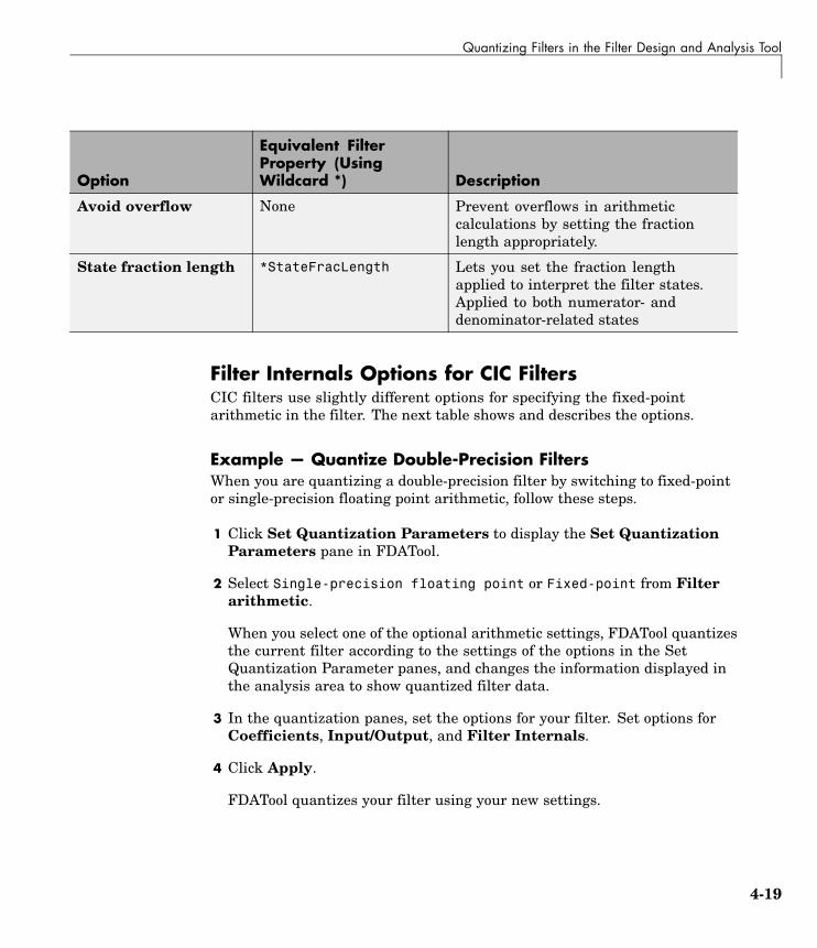
Quantizing Filters in the Filter Design and Analysis Tool
Option
Equivalent FilterProperty (UsingWildcard *) Description
Avoid overflow None Prevent overflows in arithmeticcalculations by setting the fractionlength appropriately.
State fraction length *StateFracLength Lets you set the fraction lengthapplied to interpret the filter states.Applied to both numerator- anddenominator-related states
Filter Internals Options for CIC FiltersCIC filters use slightly different options for specifying the fixed-pointarithmetic in the filter. The next table shows and describes the options.
Example — Quantize Double-Precision FiltersWhen you are quantizing a double-precision filter by switching to fixed-pointor single-precision floating point arithmetic, follow these steps.
1 Click Set Quantization Parameters to display the Set QuantizationParameters pane in FDATool.
2 Select Single-precision floating point or Fixed-point from Filterarithmetic.
When you select one of the optional arithmetic settings, FDATool quantizesthe current filter according to the settings of the options in the SetQuantization Parameter panes, and changes the information displayed inthe analysis area to show quantized filter data.
3 In the quantization panes, set the options for your filter. Set options forCoefficients, Input/Output, and Filter Internals.
4 Click Apply.
FDATool quantizes your filter using your new settings.
4-19

4 Using FDATool with Filter Design Toolbox
5 Use the analysis features in FDATool to determine whether your newquantized filter meets your requirements.
Example — Change the Quantization Properties of QuantizedFiltersWhen you are changing the settings for the quantization of a quantized filter,or after you import a quantized filter from your MATLAB workspace, followthese steps to set the property values for the filter:
1 Verify that the current filter is quantized.
2 Click Set Quantization Parameters to display the Set QuantizationParameters panel.
3 Review and select property settings for the filter quantization:Coefficients, Input/Output, and Filter Internals. Settings for optionson these panes determine how your filter quantizes data during filteringoperations.
4 Click Apply to update your current quantized filter to use the newquantization property settings from Step 3.
5 Use the analysis features in FDATool to determine whether your newquantized filter meets your requirements.
4-20
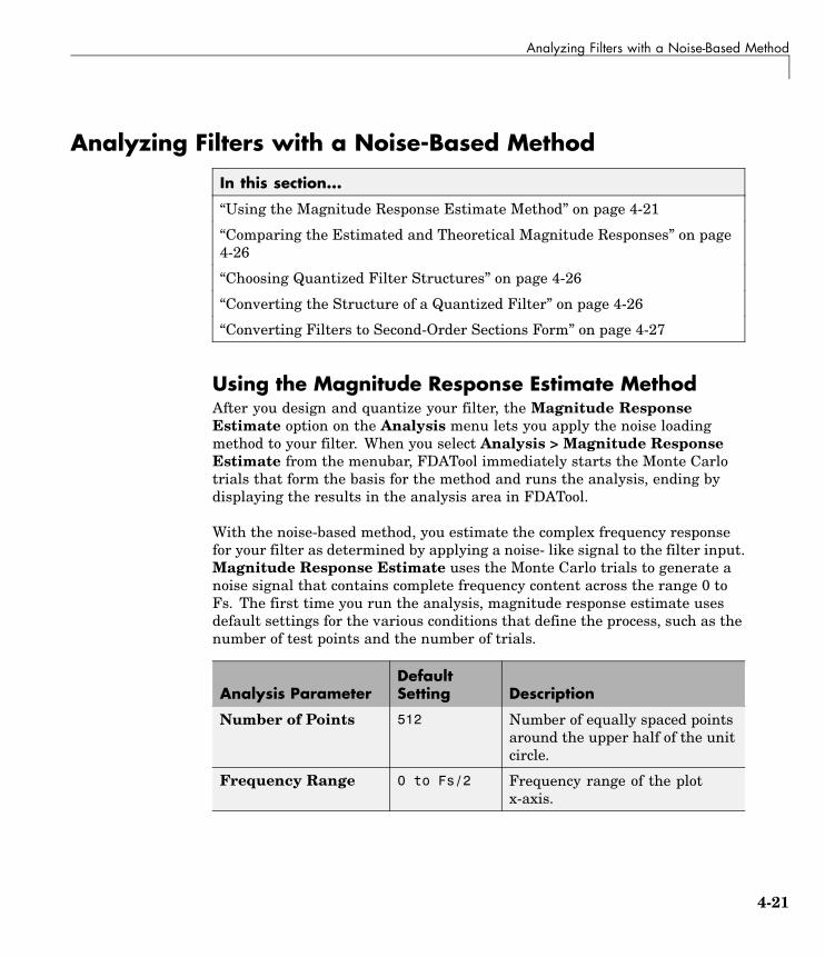
Analyzing Filters with a Noise-Based Method
Analyzing Filters with a Noise-Based Method
In this section...
“Using the Magnitude Response Estimate Method” on page 4-21
“Comparing the Estimated and Theoretical Magnitude Responses” on page4-26
“Choosing Quantized Filter Structures” on page 4-26
“Converting the Structure of a Quantized Filter” on page 4-26
“Converting Filters to Second-Order Sections Form” on page 4-27
Using the Magnitude Response Estimate MethodAfter you design and quantize your filter, the Magnitude ResponseEstimate option on the Analysis menu lets you apply the noise loadingmethod to your filter. When you select Analysis > Magnitude ResponseEstimate from the menubar, FDATool immediately starts the Monte Carlotrials that form the basis for the method and runs the analysis, ending bydisplaying the results in the analysis area in FDATool.
With the noise-based method, you estimate the complex frequency responsefor your filter as determined by applying a noise- like signal to the filter input.Magnitude Response Estimate uses the Monte Carlo trials to generate anoise signal that contains complete frequency content across the range 0 toFs. The first time you run the analysis, magnitude response estimate usesdefault settings for the various conditions that define the process, such as thenumber of test points and the number of trials.
Analysis ParameterDefaultSetting Description
Number of Points 512 Number of equally spaced pointsaround the upper half of the unitcircle.
Frequency Range 0 to Fs/2 Frequency range of the plotx-axis.
4-21

4 Using FDATool with Filter Design Toolbox
Analysis ParameterDefaultSetting Description
Frequency Units Hz Units for specifying the frequencyrange.
Sampling Frequency 48000 Inverse of the sampling period.
Frequency Scale dB Units used for the y-axis displayof the output.
NormalizedFrequency
Off Use normalized frequency for thedisplay.
After your first analysis run ends, open the Analysis Parameters dialog boxand adjust your settings appropriately, such as changing the number of trialsor number of points.
To open the Analysis Parameters dialog box, use either of the nextprocedures when you have a quantized filter in FDATool:
• Select Analysis > Analysis Parameters from the menu bar
• Right-click in the filter analysis area and select Analysis Parametersfrom the context menu
Whichever option you choose opens the dialog box as shown in the figure.Notice that the settings for the options reflect the defaults.
4-22

Analyzing Filters with a Noise-Based Method
Example — Noise Method Applied to a FilterTo demonstrate the magnitude response estimate method, start by creatinga quantized filter. For this example, use FDATool to design a sixth-orderButterworth IIR filter.
To Use Noise-Based Analysis in FDATool
1 Enter fdatool at the MATLAB prompt to launch FDATool.
2 Under Response Type, select Highpass.
3 Select IIR in Design Method. Then select Butterworth.
4 To set the filter order to 6, select Specify order under Filter Order.Enter 6 in the text box.
5 Click Design Filter.
In FDATool, the analysis area changes to display the magnitude responsefor your filter.
6 To generate the quantized version of your filter, using default quantizersettings, click on the side bar.
4-23

4 Using FDATool with Filter Design Toolbox
FDATool switches to quantization mode and displays the quantizationpanel.
7 From Filter arithmetic, select fixed-point.
Now the analysis areas shows the magnitude response for both filters —your original filter and the fixed-point arithmetic version.
8 Finally, to use noise-based estimation on your quantized filter, selectAnalysis > Magnitude Response Estimate from the menubar.
FDATool runs the trial, calculates the estimated magnitude response for thefilter, and displays the result in the analysis area as shown in this figure.
In the above figure you see the magnitude response as estimated by theanalysis method.
To View the Noise Power SpectrumWhen you use the noise method to estimate the magnitude response of a filter,FDATool simulates and applies a spectrum of noise values to test your filterresponse. While the simulated noise is essentially white, you might want tosee the actual spectrum that FDATool used to test your filter.
4-24

Analyzing Filters with a Noise-Based Method
From the Analysis menu bar option, select Round-off Noise PowerSpectrum. In the analysis area in FDATool, you see the spectrum of thenoise used to estimate the filter response. The details of the noise spectrum,such as the range and number of data points, appear in the AnalysisParameters dialog box.
To Change Your Noise Analysis ParametersIn “Example — Noise Method Applied to a Filter” on page 4-23, you usedsynthetic white noise to estimate the magnitude response for a fixed-pointhighpass Butterworth filter. Since you ran the estimate only once in FDATool,your noise analysis used the default analysis parameters settings shown in“Using the Magnitude Response Estimate Method” on page 4-21.
To change the settings, follow these steps after the first time you use thenoise estimate on your quantized filter.
1 With the results from running the noise estimating method displayed inthe FDATool analysis area, select Analysis > Analysis Parameters fromthe menubar.
To give you access to the analysis parameters, the Analysis Parametersdialog box opens as shown here (with default settings).
2 To use more points in the spectrum to estimate the magnitude response,change Number of Points to 1024 and click OK to run the analysis.
4-25

4 Using FDATool with Filter Design Toolbox
FDATool closes the Analysis Parameters dialog box and reruns the noiseestimate, returning the results in the analysis area.
To rerun the test without closing the dialog box, press Enter after you typeyour new value into a setting, then click Apply. Now FDATool runs thetest without closing the dialog box. When you want to try many differentsettings for the noise-based analysis, this is a useful shortcut.
Comparing the Estimated and Theoretical MagnitudeResponsesAn important measure of the effectiveness of the noise method for estimatingthe magnitude response of a quantized filter is to compare the estimatedresponse to the theoretical response.
One way to do this comparison is to overlay the theoretical response on theestimated response. While you have the Magnitude Response Estimatedisplaying in FDATool, select Analysis > Overlay Analysis from the menubar. Then select Magnitude Response to show both response curves plottedtogether in the analysis area.
Choosing Quantized Filter StructuresFDATool lets you change the structure of any quantized filter. Use theConvert structure option to change the structure of your filter to one thatmeets your needs.
To learn about changing the structure of a filter in FDATool, refer to“Converting to a New Structure” in your Signal Processing Toolboxdocumentation.
Converting the Structure of a Quantized FilterYou use the Convert structure option to change the structure of filter. Whenthe Source is Designed(Quantized) or Imported(Quantized), Convertstructure lets you recast the filter to one of the following structures:
• “Direct Form II Transposed Filter Structure” on page 6-52
• “Direct Form I Transposed Filter Structure” on page 6-49
4-26
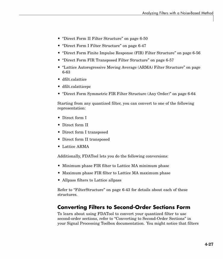
Analyzing Filters with a Noise-Based Method
• “Direct Form II Filter Structure” on page 6-50
• “Direct Form I Filter Structure” on page 6-47
• “Direct Form Finite Impulse Response (FIR) Filter Structure” on page 6-56
• “Direct Form FIR Transposed Filter Structure” on page 6-57
• “Lattice Autoregressive Moving Average (ARMA) Filter Structure” on page6-63
• dfilt.calattice
• dfilt.calatticepc
• “Direct Form Symmetric FIR Filter Structure (Any Order)” on page 6-64
Starting from any quantized filter, you can convert to one of the followingrepresentation:
• Direct form I
• Direct form II
• Direct form I transposed
• Direct form II transposed
• Lattice ARMA
Additionally, FDATool lets you do the following conversions:
• Minimum phase FIR filter to Lattice MA minimum phase
• Maximum phase FIR filter to Lattice MA maximum phase
• Allpass filters to Lattice allpass
Refer to “FilterStructure” on page 6-43 for details about each of thesestructures.
Converting Filters to Second-Order Sections FormTo learn about using FDATool to convert your quantized filter to usesecond-order sections, refer to “Converting to Second-Order Sections” inyour Signal Processing Toolbox documentation. You might notice that filters
4-27

4 Using FDATool with Filter Design Toolbox
you design in FDATool, rather than filters you imported, are implementedin SOS form.
To View Filter Structures in FDAToolTo open the demonstration, click Help > Show filter structures. After theHelp browser opens, you see the reference page for the current filter. You findthe filter structure signal flow diagram on this reference page, or you cannavigate to reference pages for other filter.
4-28

Scaling Second-Order Section Filters
Scaling Second-Order Section Filters
In this section...
“Using the Reordering and Scaling Second-Order Sections Dialog Box” onpage 4-29
“Example — Scale an SOS Filter” on page 4-31
Using the Reordering and Scaling Second-OrderSections Dialog BoxFDATool provides the ability to scale SOS filters after you create them. Usingoptions on the Reordering and Scaling Second-Order Sections dialog box,FDATool scales either or both the filter numerators and filter scale valuesaccording to your choices for the scaling options.
4-29
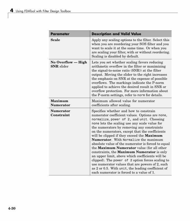
4 Using FDATool with Filter Design Toolbox
Parameter Description and Valid Value
Scale Apply any scaling options to the filter. Select thiswhen you are reordering your SOS filter and youwant to scale it at the same time. Or when youare scaling your filter, with or without reordering.Scaling is disabled by default.
No Overflow — HighSNR slider
Lets you set whether scaling favors reducingarithmetic overflow in the filter or maximizingthe signal-to-noise ratio (SNR)) at the filteroutput. Moving the slider to the right increasesthe emphasis on SNR at the expense of possibleoverflows. The markings indicate the P-normapplied to achieve the desired result in SNR oroverflow protection. For more information aboutthe P-norm settings, refer to norm for details.
MaximumNumerator
Maximum allowed value for numeratorcoefficients after scaling.
NumeratorConstraint
Specifies whether and how to constrainnumerator coefficient values. Options are none,normalize, power of 2, and unit. Choosingnone lets the scaling use any scale value forthe numerators by removing any constraintson the numerators, except that the coefficientswill be clipped if they exceed the MaximumNumerator. With Normalize the maximumabsolute value of the numerator is forced to equalthe Maximum Numerator value (for all otherconstraints, the Maximum Numerator is onlyan upper limit, above which coefficients will beclipped). The power of 2 option forces scaling touse numerator values that are powers of 2, suchas 2 or 0.5. With unit, the leading coefficient ofeach numerator is forced to a value of 1.
4-30

Scaling Second-Order Section Filters
Parameter Description and Valid Value
Overflow Mode Sets the way the filter handles arithmeticoverflow situations during scaling. Choosefrom either saturate (limit the output to thelargest positive or negative representable value)or wrap (set overflowing values to the nearestrepresentable value using modular arithmetic.
Scale ValueConstraint
Specify whether to constrain the filter scalevalues, and how to constrain them. Valid optionsare unit, power of 2, and none. Choosing unitfor the constraint disables the Max. ScaleValue setting and forces scale values to equal1. Power of 2 constrains the scale values to bepowers of 2, such as 2 or 0.5, while none removesany constraint on the scale values, except thatthey cannot exceed the Max. Scale Value.
Max. Scale Value Sets the maximum allowed scale values. SOSfilter scaling applies the Max. Scale Value limitonly when you set Scale Value Constraint toa value other than unit (the default setting).Setting a maximum scale value removes anyother limits on the scale values.
Revert to Original Filter Returns your filter to the original scaling. Beingable to revert to your original filter makes iteasier to assess the results of scaling your filter.
Various combinations of settings let you scale filter numerators withoutchanging the scale values, or adjust the filter scale values without changingthe numerators. There is no scaling control for denominators.
Example — Scale an SOS FilterStart the process by designing a lowpass elliptical filter in FDATool.
1 Launch FDATool.
2 In Response Type, select Lowpass.
4-31
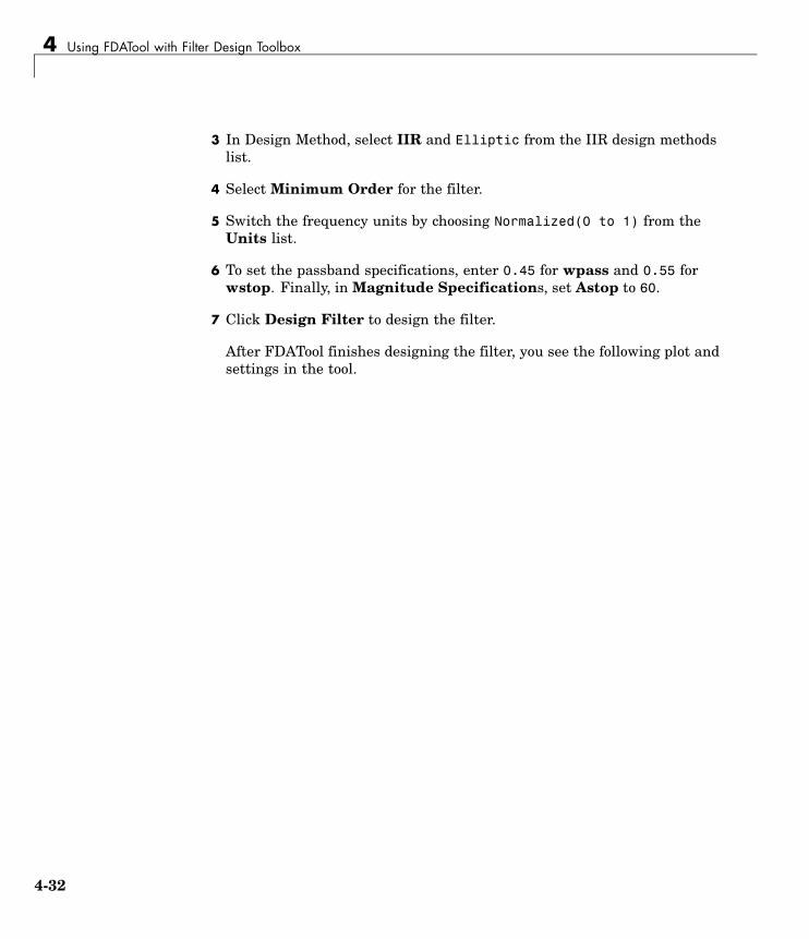
4 Using FDATool with Filter Design Toolbox
3 In Design Method, select IIR and Elliptic from the IIR design methodslist.
4 Select Minimum Order for the filter.
5 Switch the frequency units by choosing Normalized(0 to 1) from theUnits list.
6 To set the passband specifications, enter 0.45 for wpass and 0.55 forwstop. Finally, in Magnitude Specifications, set Astop to 60.
7 Click Design Filter to design the filter.
After FDATool finishes designing the filter, you see the following plot andsettings in the tool.
4-32
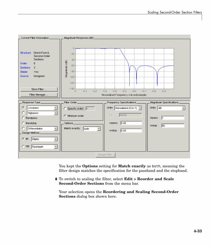
Scaling Second-Order Section Filters
You kept the Options setting for Match exactly as both, meaning thefilter design matches the specification for the passband and the stopband.
8 To switch to scaling the filter, select Edit > Reorder and ScaleSecond-Order Sections from the menu bar.
Your selection opens the Reordering and Scaling Second-OrderSections dialog box shown here.
4-33
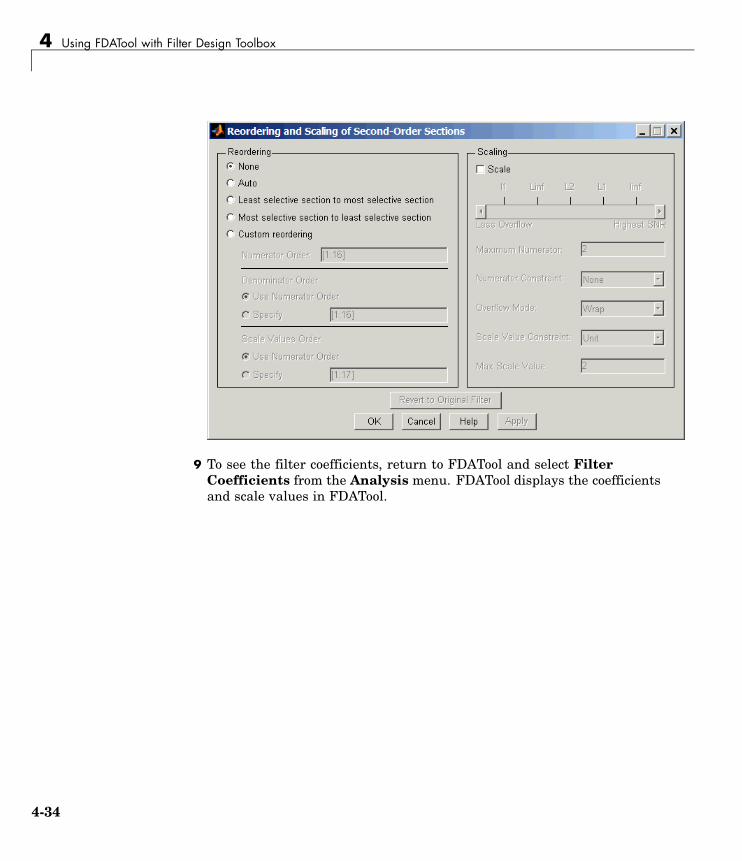
4 Using FDATool with Filter Design Toolbox
9 To see the filter coefficients, return to FDATool and select FilterCoefficients from the Analysis menu. FDATool displays the coefficientsand scale values in FDATool.
4-34
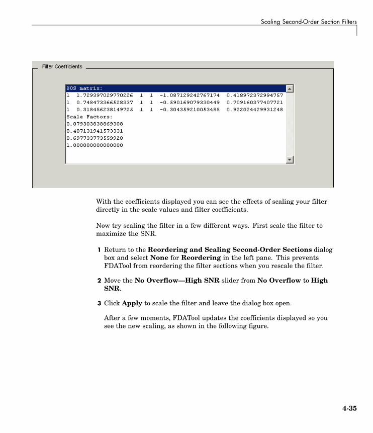
Scaling Second-Order Section Filters
With the coefficients displayed you can see the effects of scaling your filterdirectly in the scale values and filter coefficients.
Now try scaling the filter in a few different ways. First scale the filter tomaximize the SNR.
1 Return to the Reordering and Scaling Second-Order Sections dialogbox and select None for Reordering in the left pane. This preventsFDATool from reordering the filter sections when you rescale the filter.
2 Move the No Overflow—High SNR slider from No Overflow to HighSNR.
3 Click Apply to scale the filter and leave the dialog box open.
After a few moments, FDATool updates the coefficients displayed so yousee the new scaling, as shown in the following figure.
4-35

4 Using FDATool with Filter Design Toolbox
All of the scale factors are now 1, and the SOS matrix of coefficients showsthat none of the numerator coefficients are 1 and the first denominatorcoefficient of each section is 1.
4 Click Revert to Original Filter to restore the filter to the originalsettings for scaling and coefficients.
4-36

Reordering the Sections of Second-Order Section Filters
Reordering the Sections of Second-Order Section Filters
Switching FDATool to Reorder FiltersFDATool design most discrete-time filters in second-order sections. Generally,SOS filters resist the effects of quantization changes when you createfixed-point filters. After you have a second-order section filter in FDATool,either one you designed in the tool, or one you imported, FDATool providesthe capability to change the order of the sections that compose the filter. AnySOS filter in FDATool allows reordering of the sections.
To reorder the sections of a filter, you access the Reorder and Scaling ofSecond-Order Sections dialog box in FDATool.
With your SOS filter in FDATool, select Edit > Reorder and Scale fromthe menu bar. FDATool returns the reordering dialog box shown here withthe default settings.
4-37

4 Using FDATool with Filter Design Toolbox
Controls on the Reordering and Scaling of Second-Order Sections dialog box
In this dialog box, the left-hand side contains options for reordering SOSfilters. On the right you see the scaling options. These are independent —reordering your filter does not require scaling (note the Scale option) andscaling does not require that you reorder your filter (note the None optionunder Reordering). For more about scaling SOS filters, refer to “ScalingSecond-Order Section Filters” on page 4-29 and to scale in the referencesection.
Reordering SOS filters involves using the options in the Reordering andScaling of Second-Order Sections dialog box. The following table listseach reorder option and provides a description of what the option does.
4-38

Reordering the Sections of Second-Order Section Filters
Control Option Description
Auto Reorders the filter sections to minimize the outputnoise power of the filter. Note that differentordering applies to each specification type, such aslowpass or highpass. Automatic ordering adapts tothe specification type of your filter.
None Does no reordering on your filter. SelectingNone lets you scale your filter without applyingreordering at the same time. When you access thisdialog box with a current filter, this is the defaultsetting — no reordering is applied.
Least selectivesection to mostselective section
Rearranges the filter sections so the leastrestrictive (lowest Q) section is the first sectionand the most restrictive (highest Q) section is thelast section.
Most selectivesection to leastselective section
Rearranges the filter sections so the mostrestrictive (highest Q) section is the first sectionand the least restrictive (lowest Q) section is thelast section.
Custom reordering Lets you specify the section ordering to use byenabling the Numerator Order and DenominatorOrder options
Numerator Order Specify new ordering for the sections of your SOSfilter. Enter a vector of the indices of the sectionsin the order in which to rearrange them. Forexample, a filter with five sections has indices 1,2, 3, 4, and 5. To switch the second and fourthsections, the vector would be [1,4,3,2,5].
Use NumeratorOrder
Rearranges the denominators in the order assignedto the numerators.
4-39

4 Using FDATool with Filter Design Toolbox
Control Option Description
Specify Lets you specify the order of the denominators,rather than using the numerator order. Enter avector of the indices of the sections to specify theorder of the denominators to use. For example, afilter with five sections has indices 1, 2, 3, 4, and5. To switch the second and fourth sections, thevector would be [1,4,3,2,5].
Use NumeratorOrder
Reorders the scale values according to the orderof the numerators.
Specify Lets you specify the order of the scale values,rather than using the numerator order. Enter avector of the indices of the sections to specify theorder of the denominators to use. For example, afilter with five sections has indices 1, 2, 3, 4, and5. To switch the second and fourth sections, thevector would be [1,4,3,2,5].
Revert to OriginalFilter
Returns your filter to the original section ordering.Being able to revert to your original filter makescomparing the results of changing the order of thesections easier to assess.
Example — Reorder an SOS FilterWith FDATool open and a second-order filter as the current filter, you use thefollowing process to access the reordering capability and reorder you filter.Start by launching FDATool from the command prompt.
1 Enter fdatool at the command prompt to launch FDATool.
2 Design a lowpass Butterworth filter with order 10 and the defaultfrequency specifications by entering the following settings:
• Under Response Type select Lowpass.
• Under Design Method, select IIR and Butterworth from the list.
• Specify the order equal to 10 in Specify order under Filter Order.
• Keep the default Fs and Fc values in Frequency Specifications.
4-40

Reordering the Sections of Second-Order Section Filters
3 Click Design Filter.
FDATool design the Butterworth filter and returns your filter as aDirect-Form II filter implemented with second-order sections. You see thespecifications in the Current Filter Information area.
With the second-order filter in FDATool, reordering the filter uses theReordering and Scaling of Second-Order Sections feature in FDATool(also available in Filter Visualization Tool, fvtool).
4 To reorder your filter, select Edit > Reorder and Scale Second-OrderSections from the FDATool menus. FDATool opens the following dialogbox that controls reordering of the sections of your filter.
Now you are ready to reorder the sections of your filter. Note that FDAToolperforms the reordering on the current filter in the session.
4-41
4 Using FDATool with Filter Design Toolbox
Use Least Selective to Most Selective Section ReorderingTo let FDATool reorder your filter so the least selective section is first and themost selective section is last, perform the following steps in the Reorderingand Scaling of Second-Order Sections dialog box.
1 In Reordering, select Least selective section to most selectivesection.
2 To prevent filter scaling at the same time, clear Scale in Scaling.
3 In FDATool, select View > SOS View from the menu bar so you see thesections of your filter displayed in FDATool.
4 In the SOS View dialog box, select Individual sections. Making thischoice configures FDATool to show the magnitude response curves for eachsection of your filter in the analysis area.
5 Back in the Reordering and Scaling of Second-Order Sections dialogbox, click Apply to reorder your filter according to the Qs of the filtersections, and keep the dialog box open. In response, FDATool presentsthe responses for each filter section (there should be five sections) in theanalysis area.
4-42

Reordering the Sections of Second-Order Section Filters
In the next two figures you can compare the ordering of the sections ofyour filter. In the first figure, your original filter sections appear. In thesecond figure, the sections have been rearranged from least selective tomost selective.
You see what reordering does, although the result is a bit subtle. Now trycustom reordering the sections of your filter or using the most selective toleast selective reordering option.
4-43

4 Using FDATool with Filter Design Toolbox
Viewing SOS Filter Sections
In this section...
“Using the SOS View Dialog Box” on page 4-44
“Example — View the Sections of SOS Filters” on page 4-47
Using the SOS View Dialog BoxSince you can design and reorder the sections of SOS filters, FDATool providesthe ability to view the filter sections in the analysis area — SOS View. Onceyou have a second-order section filter as your current filter in FDATool,you turn on the SOS View option to see the filter sections individually, orcumulatively, or even only some of the sections. Enabling SOS View putsFDATool in a mode where all second-order section filters display sections untilyou disable the SOS View option. SOS View mode applies to any analysis youdisplay in the analysis area. For example, if you configure FDATool to showthe phase responses for filters, enabling SOS View means FDATool displaysthe phase response for each section of SOS filters.
Controls on the SOS View Dialog Box
SOS View uses a few options to control how FDATool displays the sections,or which sections to display. When you select View > SOS View from theFDATool menu bar, you see this dialog box containing options to configureSOS View operation.
4-44

Viewing SOS Filter Sections
By default, SOS View shows the overall response of SOS filters. Options inthe SOS View dialog box let you change the display. This table lists all theoptions and describes the effects of each.
Option Description
Overall Filter This is the familiar display in FDATool. Fora second-order section filter you see only theoverall response rather than the responses forthe individual sections. This is the defaultconfiguration.
Individual sections When you select this option, FDATool displaysthe response for each section as a curve.If your filter has five sections you see fiveresponse curves, one for each section, and theyare independent. Compare to Cumulativesections.
4-45

4 Using FDATool with Filter Design Toolbox
Option Description
Cumulative sections When you select this option, FDATooldisplays the response for each section as theaccumulated response of all prior sections inthe filter. If your filter has five sections you seefive response curves:
• The first curve plots the response for thefirst filter section.
• The second curve plots the response for thecombined first and second sections.
• The third curve plots the response for thefirst, second, and third sections combined.
And so on until all filter sections appear in thedisplay. The final curve represents the overallfilter response. Compare to Cumulativesections and Overall Filter.
4-46

Viewing SOS Filter Sections
Option Description
User defined Here you define which sections to display, andin which order. Selecting this option enablesthe text box where you enter a cell array ofthe indices of the filter sections. Each indexrepresents one section. Entering one indexplots one response. Entering something like{1:2} plots the combined response of sections 1and 2. If you have a filter with four sections,the entry {1:4} plots the combined response forall four sections, whereas {1,2,3,4} plots theresponse for each section. Note that after youenter the cell array, you need to click OK orApply to update the FDATool analysis area tothe new SOS View configuration.
Use secondary-scalingpoints
This directs FDATool to use the secondaryscaling points in the sections to determinewhere to split the sections. This option appliesonly when the filter is a df2sos or df1tsosfilter. For these structures, the secondaryscaling points refer to the scaling locationsbetween the recursive and the nonrecursiveparts of the section (the "middle" of the section).By default, secondary-scaling points is notenabled. You use this with the Cumulativesections option only.
Example — View the Sections of SOS FiltersAfter you design or import an SOS filter in to FDATool, the SOS view optionlets you see the per section performance of your filter. Enabling SOS Viewfrom the View menu in FDATool configures the tool to display the sections ofSOS filters whenever the current filter is an SOS filter.
These next steps demonstrate using SOS View to see your filter sectionsdisplayed in FDATool.
1 Launch FDATool.
4-47

4 Using FDATool with Filter Design Toolbox
2 Create a lowpass SOS filter using the Butterworth design method. Specifythe filter order to be 6. Using a low order filter makes seeing the sectionsmore clear.
3 Design your new filter by clicking Design Filter.
FDATool design your filter and show you the magnitude response in theanalysis area. In Current Filter Information you see the specifications foryour filter. You should have a sixth-order Direct-Form II, Second-OrderSections filter with three sections.
4 To enable SOS View, select View > SOS View from the menu bar.
Now you see the SOS View dialog box in FDATool. Options here let youspecify how to display the filter sections.
By default the analysis area in FDATool shows the overall filter response,not the individual filter section responses. This dialog box lets you changethe display configuration to see the sections.
5 To see the magnitude responses for each filter section, select Individualsections.
4-48

Viewing SOS Filter Sections
6 Click Apply to update FDATool to display the responses for each filtersection. The analysis area changes to show you something like thefollowing figure.
If you switch FDATool to display filter phase responses, you see the phaseresponse for each filter section in the analysis area.
7 To define your own display of the sections, you use the User definedoption and enter a vector of section indices to display. Now you see a
4-49
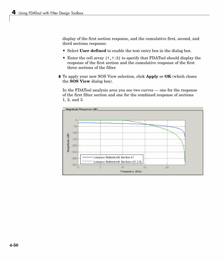
4 Using FDATool with Filter Design Toolbox
display of the first section response, and the cumulative first, second, andthird sections response:
• Select User defined to enable the text entry box in the dialog box.
• Enter the cell array {1,1:3} to specify that FDATool should display theresponse of the first section and the cumulative response of the firstthree sections of the filter.
8 To apply your new SOS View selection, click Apply or OK (which closesthe SOS View dialog box).
In the FDATool analysis area you see two curves — one for the responseof the first filter section and one for the combined response of sections1, 2, and 3.
4-50

Importing and Exporting Quantized Filters
Importing and Exporting Quantized Filters
In this section...
“Overview and Structures” on page 4-51
“Example — Import Quantized Filters” on page 4-52
“To Export Quantized Filters” on page 4-53
Overview and StructuresWhen you import a quantized filter into FDATool, or export a quantized filterfrom FDATool to your workspace, the import and export functions use objectsand you specify the filter as a variable. This contrasts with importing andexporting nonquantized filters, where you select the filter structure and enterthe filter numerator and denominator for the filter transfer function.
You have the option of exporting quantized filters to your MATLAB workspace,exporting them to text files, or exporting them to MAT-files.
For general information about importing and exporting filters in FDATool,refer to “FDATool: A Filter Design and Analysis GUI” in the Signal ProcessingToolbox User’s Guide.
FDATool imports quantized filters having the following structures:
• Direct form I
• Direct form II
• Direct form I transposed
• Direct form II transposed
• Direct form symmetric FIR
• Direct form antisymmetric FIR
• Lattice allpass
• Lattice AR
• Lattice MA minimum phase
4-51

4 Using FDATool with Filter Design Toolbox
• Lattice MA maximum phase
• Lattice ARMA
• Lattice coupled-allpass
• Lattice coupled-allpass power complementary
Example — Import Quantized FiltersAfter you design or open a quantized filter in your MATLAB workspace,FDATool lets you import the filter for analysis. Follow these steps to importyour filter in to FDATool:
1 Open FDATool.
2 Select Filter > Import Filter from the menu bar.
In the lower region of FDATool, the Design Filter pane becomes ImportFilter, and options appear for importing quantized filters, as shown.
3 From the Filter Structure list, select Filter object.
The options for importing filters change to include:
• Discrete filter — Enter the variable name for the discrete-time,fixed-point filter in your workspace.
4-52

Importing and Exporting Quantized Filters
• Frequency units — Select the frequency units from the Units listunder Sampling Frequency, and specify the sampling frequency valuein Fs if needed. Your sampling frequency must correspond to the unitsyou select. For example, when you select Normalized (0 to 1), Fsdefaults to one. But if you choose one of the frequency options, enter thesampling frequency in your selected units. If you have the samplingfrequency defined in your workspace as a variable, enter the variablename for the sampling frequency.
4 Click Import to import the filter.
FDATool checks your workspace for the specified filter. It imports the filterif it finds it, displaying the magnitude response for the filter in the analysisarea. If it cannot find the filter it returns an FDATool Error dialog box.
Note If, during any FDATool session, you switch to quantization modeand create a fixed-point filter, FDATool remains in quantization mode.If you import a double-precision filter, FDATool automatically quantizesyour imported filter applying the most recent quantization parameters.When you check the current filter information for your imported filter, itwill indicate that the filter is Source: imported (quantized) even thoughyou did not import a quantized filter.
To Export Quantized FiltersTo save your filter design, FDATool lets you export the quantized filter toyour MATLAB workspace (or you can save the current session in FDATool).When you choose to save the quantized filter by exporting it, you select oneof these options:
• Export to your MATLAB workspace
• Export to a text file
• Export to a MAT-file
Example — Export Coefficients or Objects to the WorkspaceYou can save the filter as filter coefficients variables or as a dfilt filter objectvariable. To save the filter to the MATLAB workspace:
4-53

4 Using FDATool with Filter Design Toolbox
1 Select Export from the File menu. The Export dialog box appears.
2 Select Workspace from the Export To list.
3 Select Coefficients from the Export As list to save the filter coefficientsor select Objects to save the filter in a filter object.
4 For coefficients, assign variable names using the Numerator andDenominator options under Variable Names. For objects, assignthe variable name in the Discrete or Quantized filter option. If youhave variables with the same names in your workspace and you want tooverwrite them, select the Overwrite Variables box.
5 Click the OK button
If you try to export the filter to a variable name that exists in yourworkspace, and you did not select Overwrite existing variables,FDATool stops the export operation and returns a warning that the variableyou specified as the quantized filter name already exists in the workspace.To continue to export the filter to the existing variable, click OK to dismissthe warning dialog box, select the Overwrite existing variables checkbox and click OK or Apply.
Getting Filter Coefficients After ExportingTo extract the filter coefficients from your quantized filter after you exportthe filter to MATLAB, use the celldisp function in MATLAB. For example,create a quantized filter in FDATool and export the filter as Hq. To extract thefilter coefficients for Hq, use
celldisp(Hq.referencecoefficients)
which returns the cell array containing the filter reference coefficients, or
celldisp(Hq.quantizedcoefficients
to return the quantized coefficients.
Example — Exporting as a Text FileTo save your quantized filter as a text file, follow these steps:
4-54

Importing and Exporting Quantized Filters
1 Select Export from the File menu.
2 Select Text-file under Export to.
3 Click OK to export the filter and close the dialog box. Click Apply to exportthe filter without closing the Export dialog box. Clicking Apply letsyou export your quantized filter to more than one name without leavingthe Export dialog box.
The Export Filter Coefficients to Text-file dialog box appears. This isthe standard Microsoft Windows save file dialog box.
4 Choose or enter a directory and filename for the text file and click OK.
FDATool exports your quantized filter as a text file with the name youprovided, and the MATLAB editor opens, displaying the file for editing.
Example — Exporting as a MAT-FileTo save your quantized filter as a MAT-file, follow these steps:
1 Select Export from the File menu.
2 Select MAT-file under Export to.
3 Assign a variable name for the filter.
4 Click OK to export the filter and close the dialog box. Click Apply to exportthe filter without closing the Export dialog box. Clicking Apply letsyou export your quantized filter to more than one name without leavingthe Export dialog box.
The Export Filter Coefficients to MAT-file dialog box appears. This isthe standard Microsoft Windows save file dialog box.
5 Choose or enter a directory and filename for the text file and click OK.
FDATool exports your quantized filter as a MAT-file with the specifiedname.
4-55

4 Using FDATool with Filter Design Toolbox
Importing XILINX Coefficient (.COE) Files
Example — Import XILINX .COE FilesYou can import XILINX coefficients (.coe) files into FDATool to createquantized filters directly using the imported filter coefficients.
To use the import file feature:
1 Select File > Import Filter From XILINX Coefficient (.COE) Filein FDATool.
2 In the Import Filter From XILINX Coefficient (.COE) File dialog box,find and select the .coe file to import.
3 Click Open to dismiss the dialog box and start the import process.
FDATool imports the coefficient file and creates a quantized, single-section,direct-form FIR filter.
4-56

Transforming Filters
Transforming Filters
In this section...
“FDATool Filter Transformation Capabilities” on page 4-57
“Original Filter Type” on page 4-58
“Frequency Point to Transform” on page 4-62
“Transformed Filter Type” on page 4-63
“Specify Desired Frequency Location” on page 4-63
FDATool Filter Transformation CapabilitiesThe toolbox provides functions for transforming filters between various forms.When you use FDATool with the toolbox installed, a side bar button and amenu bar option enable you to use the Transform Filter panel to transformfilters as well as using the command line functions.
From the selection on the FDATool menu bar — Transformations — you cantransform lowpass FIR and IIR filters to a variety of passband shapes.
You can convert your FIR filters from:
• Lowpass to lowpass.
• Lowpass to highpass.
For IIR filters, you can convert from:
• Lowpass to lowpass.
• Lowpass to highpass.
• Lowpass to bandpass.
• Lowpass to bandstop.
When you click the Transform Filter button, , on the side bar, theTransform Filter panel opens in FDATool, as shown here.
4-57

4 Using FDATool with Filter Design Toolbox
Your options for Original filter type refer to the type of your current filterto transform. If you select lowpass, you can transform your lowpass filterto another lowpass filter or to a highpass filter, or to numerous other filterformats, real and complex.
Note When your original filter is an FIR filter, both the FIR and IIRtransformed filter type options appear on the Transformed filter type list.Both options remain active because you can apply the IIR transforms to anFIR filter. If your source is as IIR filter, only the IIR transformed filter optionsshow on the list.
Original Filter TypeSelect the magnitude response of the filter you are transforming from the list.Your selection changes the types of filters you can transform to. For example:
• When you select Lowpass with an IIR filter, your transformed filter typecan be
- Lowpass
- Highpass
- Bandpass
- Bandstop
- Multiband
4-58

Transforming Filters
- Bandpass (complex)
- Bandstop (complex)
- Multiband (complex)
• When you select Lowpass with an FIR filter, your transformed filtertype can be
- Lowpass
- Lowpass (FIR)
- Highpass
- Highpass (FIR) narrowband
- Highpass (FIR) wideband
- Bandpass
- Bandstop
- Multiband
- Bandpass (complex)
- Bandstop (complex)
- Multiband (complex)
In the following table you see each available original filter type and all thetypes of filter to which you can transform your original.
4-59

4 Using FDATool with Filter Design Toolbox
Original Filter Available Transformed Filter Types
Lowpass FIR • Lowpass
• Lowpass (FIR)
• Highpass
• Highpass (FIR) narrowband
• Highpass (FIR) wideband
• Bandpass
• Bandstop
• Multiband
• Bandpass (complex)
• Bandstop (complex)
• Multiband (complex)
Lowpass IIR • Lowpass
• Highpass
• Bandpass
• Bandstop
• Multiband
• Bandpass (complex)
• Bandstop (complex)
• Multiband (complex)
4-60

Transforming Filters
Original Filter Available Transformed Filter Types
Highpass FIR • Lowpass
• Lowpass (FIR) narrowband
• Lowpass (FIR) wideband
• Highpass (FIR)
• Highpass
• Bandpass
• Bandstop
• Multiband
• Bandpass (complex)
• Bandstop (complex)
• Multiband (complex)
Highpass IIR • Lowpass
• Highpass
• Bandpass
• Bandstop
• Multiband
• Bandpass (complex)
• Bandstop (complex)
• Multiband (complex)
Bandpass FIR • Bandpass
• Bandpass (FIR)
Bandpass IIR Bandpass
Bandstop FIR • Bandstop
• Bandstop (FIR)
Bandstop IIR Bandstop
4-61

4 Using FDATool with Filter Design Toolbox
Note also that the transform options change depending on whether youroriginal filter is FIR or IIR. Starting from an IIR filter, you can transform toIIR or FIR forms. With an IIR original filter, you are limited to IIR targetfilters.
After selecting your response type, use Frequency point to transform tospecify the magnitude response point in your original filter to transfer toyour target filter. Your target filter inherits the performance features of youroriginal filter, such as passband ripple, while changing to the new responseform.
For more information about transforming filters, refer to “FrequencyTransformations for Real Filters” on page 3-11 and “FrequencyTransformations for Complex Filters” on page 3-26.
Frequency Point to TransformThe frequency point you enter in this field identifies a magnitude responsevalue (in dB) on the magnitude response curve.
When you enter frequency values in the Specify desired frequencylocation option, the frequency transformation tries to set the magnituderesponse of the transformed filter to the value identified by the frequencypoint you enter in this field.
While you can enter any location, generally you should specify a filterpassband or stopband edge, or a value in the passband or stopband.
The Frequency point to transform sets the magnitude response at thevalues you enter in Specify desired frequency location. Specify a valuethat lies at either the edge of the stopband or the edge of the passband.
If, for example, you are creating a bandpass filter from a highpass filter, thetransformation algorithm sets the magnitude response of the transformedfilter at the Specify desired frequency location to be the same as theresponse at the Frequency point to transform value. Thus you get abandpass filter whose response at the low and high frequency locations is thesame. Notice that the passband between them is undefined. In the next twofigures you see the original highpass filter and the transformed bandpassfilter.
4-62
Transforming Filters
For more information about transforming filters, refer to Chapter 3, “DigitalFrequency Transformations”.
Transformed Filter TypeSelect the magnitude response for the target filter from the list. The completelist of transformed filter types is:
• Lowpass
• Lowpass (FIR)
• Highpass
• Highpass (FIR) narrowband
• Highpass (FIR) wideband
• Bandpass
• Bandstop
• Multiband
• Bandpass (complex)
• Bandstop (complex)
• Multiband (complex)
Not all types of transformed filters are available for all filter types on theOriginal filter types list. You can transform bandpass filters only tobandpass filters. Or bandstop filters to bandstop filters. Or IIR filters toIIR filters.
For more information about transforming filters, refer to “FrequencyTransformations for Real Filters” on page 3-11 and “FrequencyTransformations for Complex Filters” on page 3-26.
Specify Desired Frequency LocationThe frequency point you enter in Frequency point to transformmatched a magnitude response value. At each frequency you enter here,the transformation tries to make the magnitude response the same as theresponse identified by your Frequency point to transform value.
4-63

4 Using FDATool with Filter Design Toolbox
While you can enter any location, generally you should specify a filterpassband or stopband edge, or a value in the passband or stopband.
For more information about transforming filters, refer to Chapter 3, “DigitalFrequency Transformations”.
Example — Transform FiltersTo transform the magnitude response of your filter, use the TransformFilter option on the side bar.
1 Design or import your filter into FDATool.
2 Click Transform Filter, , on the side bar.
FDATool opens the Transform Filter panel in FDATool.
3 From the Original filter type list, select the response form of the filteryou are transforming.
When you select the type, whether is lowpass, highpass, bandpass, orbandstop, FDATool recognizes whether your filter form is FIR or IIR.Using both your filter type selection and the filter form, FDATool adjuststhe entries on the Transformed filter type list to show only those thatapply to your original filter.
4-64

Transforming Filters
4 Enter the frequency point to transform value in Frequency point totransform. Notice that the value you enter must be in KHz; for example,enter 0.1 for 100 Hz or 1.5 for 1500 Hz.
5 From the Transformed filter type list, select the type of filter you wantto transform to.
Your filter type selection changes the options here.
• When you pick a lowpass or highpass filter type, you enter one value inSpecify desired frequency location.
• When you pick a bandpass or bandstop filter type, you enter two values— one in Specify desired low frequency location and one in Specifydesired high frequency location. Your values define the edges ofthe passband or stopband.
• When you pick a multiband filter type, you enter values as elements in avector in Specify a vector or desired frequency locations — one elementfor each desired location. Your values define the edges of the passbandsand stopbands.
After you click Transform Filter, FDATool transforms your filter,displays the magnitude response of your new filter, and updates theCurrent Filter Information to show you that your filter has beentransformed. In the filter information, the Source is Transformed.
For example, the figure shown here includes the magnitude responsecurves for two filter. The original filter is a lowpass filter with rolloffbetween 0.2 and 0.25. The transformed filter is a lowpass filter withrolloff region between 0.8 and 0.85.
4-65
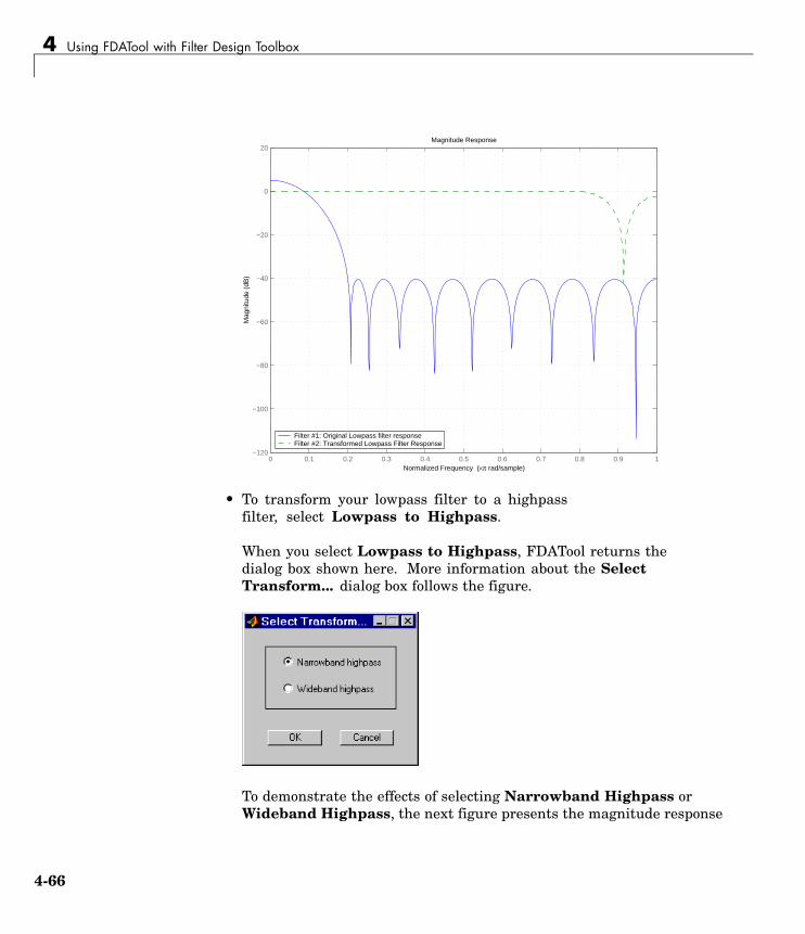
4 Using FDATool with Filter Design Toolbox
0 0.1 0.2 0.3 0.4 0.5 0.6 0.7 0.8 0.9 1−120
−100
−80
−60
−40
−20
0
20
Normalized Frequency (×π rad/sample)
Mag
nitu
de (
dB)
Magnitude Response
Filter #1: Original Lowpass filter responseFilter #2: Transformed Lowpass Filter Response
• To transform your lowpass filter to a highpassfilter, select Lowpass to Highpass.
When you select Lowpass to Highpass, FDATool returns thedialog box shown here. More information about the SelectTransform... dialog box follows the figure.
To demonstrate the effects of selecting Narrowband Highpass orWideband Highpass, the next figure presents the magnitude response
4-66

Transforming Filters
curves for a source lowpass filter after it is transformed to both narrow-and wideband highpass filters. For comparison, the response ofthe original filter appears as well.
0 0.1 0.2 0.3 0.4 0.5 0.6 0.7 0.8 0.9 1−120
−100
−80
−60
−40
−20
0
20
Normalized Frequency (×π rad/sample)
Mag
nitu
de (
dB)
Magnitude Response
Filter #1:Original Lowpass Filter ResponseFilter #2:Narrowband Highpass Filter ResponseFilter #3: Wideband Highpass Filter Response
For the narrowband case, the transformation algorithm essentiallyreverses the magnitude response, like reflecting the curve around they-axis, then translating the curve to the right until the origin lies at 1 onthe x-axis. After reflecting and translating, the passband at highfrequencies is the reverse of the passband of the original filter at lowfrequencies with the same rolloff and ripple characteristics.
4-67

4 Using FDATool with Filter Design Toolbox
Designing Multirate Filters in FDATool
In this section...
“Introduction” on page 4-68
“Switching FDATool to Multirate Filter Design Mode” on page 4-68
“Controls on the Multirate Design Panel” on page 4-69
“Quantizing Multirate Filters” on page 4-80
IntroductionNot only can you design multirate filters from the MATLAB command prompt,FDATool provides the same design capability in a graphical user interfacetool. By starting FDATool and switching to the multirate filter design modeyou have access to all of the multirate design capabilities in the toolbox —decimators, interpolators, and fractional rate changing filters, among others.
Switching FDATool to Multirate Filter Design ModeThe multirate filter design mode in FDATool lets you specify and design awide range of multirate filters, including decimators and interpolators.
With FDATool open, click Create a Multirate Filter, , on the side bar.You see FDATool switch to the design mode showing the multirate filterdesign options. Shown in the following figure is the default multirate designconfiguration that designs an interpolating filter with an interpolation factorof 2. The design uses the current FIR filter in FDATool.
4-68

Designing Multirate Filters in FDATool
When the current filter in FDATool is not an FIR filter, the multirate filterdesign panel removes the Use current FIR filter option and selects the Usedefault Nyquist FIR filter option instead as the default setting.
Controls on the Multirate Design PanelYou see the options that allow you to design a variety of multirate filters. TheType option is your starting point. From this list you select the multiratefilter to design. Based on your selection, other options change to provide thecontrols you need to specify your filter.
4-69

4 Using FDATool with Filter Design Toolbox
Notice the separate sections of the design panel. On the left is the filter typearea where you choose the type of multirate filter to design and set the filterperformance specifications.
In the center section FDATool provides choices that let you pick the filterdesign method to use.
The rightmost section offers options that control filter configuration when youselect Cascaded-Integrator Comb (CIC) as the design method in the centersection. Both the Decimator type and Interpolator type filters let you usethe Cascaded-Integrator Comb (CIC) option to design multirate filters.
Here are all the options available when you switch to multirate filter designmode. Each option listed includes a brief description of what the option doeswhen you use it.
4-70
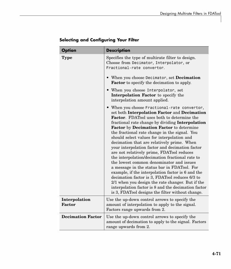
Designing Multirate Filters in FDATool
Selecting and Configuring Your Filter
Option Description
Type Specifies the type of multirate filter to design.Choose from Decimator, Interpolator, orFractional-rate convertor.
• When you choose Decimator, set DecimationFactor to specify the decimation to apply.
• When you choose Interpolator, setInterpolation Factor to specify theinterpolation amount applied.
• When you choose Fractional-rate convertor,set both Interpolation Factor and DecimationFactor. FDATool uses both to determine thefractional rate change by dividing InterpolationFactor by Decimation Factor to determinethe fractional rate change in the signal. Youshould select values for interpolation anddecimation that are relatively prime. Whenyour interpolation factor and decimation factorare not relatively prime, FDATool reducesthe interpolation/decimation fractional rate tothe lowest common denominator and issuesa message in the status bar in FDATool. Forexample, if the interpolation factor is 6 and thedecimation factor is 3, FDATool reduces 6/3 to2/1 when you design the rate changer. But if theinterpolation factor is 8 and the decimation factoris 3, FDATool designs the filter without change.
InterpolationFactor
Use the up-down control arrows to specify theamount of interpolation to apply to the signal.Factors range upwards from 2.
Decimation Factor Use the up-down control arrows to specify theamount of decimation to apply to the signal. Factorsrange upwards from 2.
4-71

4 Using FDATool with Filter Design Toolbox
Selecting and Configuring Your Filter (Continued)
Option Description
SamplingFrequency
No settings here. Just Units and Fs below.
Units Specify whether Fs is specified in Hz, kHz, MHz, GHz,or Normalized (0 to 1) units.
Fs Set the full scale sampling frequency in thefrequency units you specified in Units. When youselect Normalized for Units, you do not enter avalue for Fs.
Designing Your Filter
Option Description
Use current FIRfilter
Directs FDATool to use the current FIR filter todesign the multirate filter. If the current filter is anIIR form, you cannot select this option. You cannotdesign multirate filters with IIR structures.
Use a defaultNyquist Filter
Tells FDATool to use the default Nyquist designmethod when the current filter in FDATool is notan FIR filter.
CascadedIntegrator-Comb(CIC)
Design CIC filters using the options provided in theright-hand area of the multirate design panel.
4-72

Designing Multirate Filters in FDATool
Designing Your Filter (Continued)
Option Description
Hold Interpolator(Zero-order)
When you design an interpolator, you can specifyhow the filter sets interpolated values betweensignal values. When you select this option, theinterpolator applies the most recent signal value foreach interpolated value until it processes the nextsignal value. This is similar to sample-and-holdtechniques. Compare to the Linear Interpolatoroption.
Linear Interpolator(First-order)
When you design an interpolator, you can specifyhow the filter sets interpolated values betweensignal values. When you select this option, theinterpolator applies linear interpolation betweensignal value to set the interpolated value until itprocesses the next signal value. Compare to theLinear Interpolator option.
To see the difference between hold interpolation and linear interpolation, thefollowing figure presents a sine wave signal s1 in three forms:
• The top subplot in the figure presents signal s1 without interpolation.
• The middle subplot shows signal s1 interpolated by a linear interpolatorwith an interpolation factor of 5.
• The bottom subplot shows signal s1 interpolated by a hold interpolator withan interpolation factor of 5.
You see in the bottom figure the sample and hold nature of hold interpolation,and the first-order linear interpolation applied by the linear interpolator.
4-73

4 Using FDATool with Filter Design Toolbox
1 2 3 4 5 6 7 8 9 10−1
−0.5
0
0.5
1Uninterpolated Signal s1
0 5 10 15 20 25 30 35 40 45 50−1
−0.5
0
0.5
1First−Order Linear Interpolation By 5 of Signal s1
0 5 10 15 20 25 30 35 40 45 50−1
−0.5
0
0.5
1
Samples
Zero−Order Hold Interpolation By 5 of Signal s1
We used FDATool to create interpolators similar to the following code forthe figure:
• Linear interpolator — hm=mfilt.linearinterp(5)
• Hold interpolator — hm=mfilt.holdinterp(5)
Options for Designing CICFilters Description
Differential Delay Sets the differential delay for the CIC filter. Usually a value ofone or two is appropriate.
Number of Sections Specifies the number of sections in a CIC decimator. The defaultnumber of sections is 2 and the range is any positive integer.
4-74

Designing Multirate Filters in FDATool
Example — Design a Fractional Rate ConvertorTo introduce the process you use to design a multirate filter in FDATool, thisexample uses the options to design a fractional rate convertor which uses7/3 as the fractional rate. Begin the design by creating a default lowpassFIR filter in FDATool. You do not have to begin with this FIR filter, but thedefault filter works fine.
1 Launch FDATool.
2 Select the settings for a minimum-order lowpass FIR filter, using theEquiripple design method.
3 When FDATool displays the magnitude response for the filter, click inthe side bar. FDATool switches to multirate filter design mode, showing themultirate design panel, shown in the following figure.
4-75

4 Using FDATool with Filter Design Toolbox
4 To design a fractional rate filter, select Fractional-rate convertorfrom the Type list. The Interpolation Factor and Decimation Factoroptions become available.
5 In Interpolation Factor, use the up arrow to set the interpolation factorto 7.
6 Using the up arrow in Decimation Factor, set 3 as the decimation factor.
7 Select Use a default Nyquist FIR filter. You could design the rateconvertor with the current FIR filter as well.
4-76

Designing Multirate Filters in FDATool
8 Enter 24000 to set Fs.
9 Click Create Multirate Filter.
After designing the filter, FDATool returns with the specifications foryour new filter displayed in Current Filter Information, and showsthe magnitude response of the filter.
You can test the filter by exporting it to your workspace and using it to filtera signal. For information about exporting filters, refer to “Importing andExporting Quantized Filters” on page 4-51.
4-77

4 Using FDATool with Filter Design Toolbox
Example — Design a CIC Decimator for 8 Bit Input/Output DataAnother kind of filter you can design in FDATool is Cascaded-IntegratorComb (CIC) filters. FDATool provides the options needed to configure yourCIC to meet your needs.
1 Launch FDATool and design the default FIR lowpass filter. Designing afilter at this time is an optional step.
2 Switch FDATool to multirate design mode by clicking on the side bar.
3 For Type, select Decimator, and set Decimation Factor to 3.
4 To design the decimator using a CIC implementation, selectCascaded-Integrator Comb (CIC). This enables the CIC-related optionson the right of the panel.
5 Set Differential Delay to 2. Generally, 1 or 2 are good values to use.
6 Enter 2 for the Number of Sections. Settings in the multirate designpanel should look like this.
7 Click Create Multirate Filter.
FDATool designs the filter, shows the magnitude response in the analysisarea, and updates the current filter information to show that you designeda tenth-order cascaded-integrator comb decimator with two sections. Notice
4-78
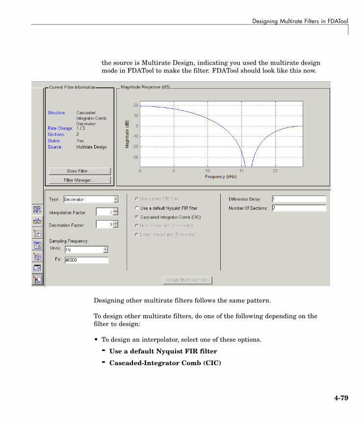
Designing Multirate Filters in FDATool
the source is Multirate Design, indicating you used the multirate designmode in FDATool to make the filter. FDATool should look like this now.
Designing other multirate filters follows the same pattern.
To design other multirate filters, do one of the following depending on thefilter to design:
• To design an interpolator, select one of these options.
- Use a default Nyquist FIR filter
- Cascaded-Integrator Comb (CIC)
4-79

4 Using FDATool with Filter Design Toolbox
- Hold Interpolator (Zero-order)
- Linear Interpolator (First-order)
• To design a decimator, select from these options.
- Use a default Nyquist FIR filter
- Cascaded-Integrator Comb (CIC)
• To design a fractional-rate convertor, select Use a default Nyquist FIRfilter.
Quantizing Multirate FiltersAfter you design a multirate filter in FDATool, the quantization featuresenable you to convert your floating-point multirate filter to fixed-pointarithmetic.
Note CIC filters are always fixed-point.
With your multirate filter as the current filter in FDATool, you can quantizeyour filter and use the quantization options to specify the fixed-pointarithmetic the filter uses.
To Quantize and Configure Multirate FiltersFollow these steps to convert your multirate filter to fixed-point arithmeticand set the fixed-point options.
1 Design or import your multirate filter and make sure it is the current filterin FDATool.
2 Click the Set Quantization Parameters button on the side bar.
3 From the Filter Arithmetic list on the Filter Arithmetic pane, selectFixed-point. If your filter is a CIC filter, the Fixed-point option isenabled by default and you do not set this option.
4 In the quantization panes, set the options for your filter. Set options forCoefficients, Input/Output, and Filter Internals.
4-80
Designing Multirate Filters in FDATool
5 Click Apply.
When you current filter is a CIC filter, the options on the Input/Output andFilter Internals panes change to provide specific features for CIC filters.
Input/OutputThe options that specify how your CIC filter uses input and output valuesare listed in the table below.
Option Name Description
Input Word Length Sets the word length used to represent the inputto a filter.
Input fractionlength
Sets the fraction length used to interpret inputvalues to filter.
Input range (+/-) Lets you set the range the inputs represent. Youuse this instead of the Input fraction lengthoption to set the precision. When you enter a valuex, the resulting range is -x to x. Range must be apositive integer.
Output word length Sets the word length used to represent the outputfrom a filter.
Avoid overflow Directs the filter to set the fraction length for theinput to prevent the output values from exceedingthe available range as defined by the word length.Clearing this option lets you set Output fractionlength.
Output fraction length Sets the fraction length used to represent outputvalues from a filter.
Output range (+/-) Lets you set the range the outputs represent. Youuse this instead of the Output fraction lengthoption to set the precision. When you enter a valuex, the resulting range is -x to x. Range must be apositive integer.
4-81

4 Using FDATool with Filter Design Toolbox
The available options change when you change the Filter precision setting.Moving from Full to Specify all adds increasing control by enabling moreinput and output word options.
Filter InternalsWith a CIC filter as your current filter, the Filter precision option on theFilter Internals pane includes modes for controlling the filter word andfraction lengths.
There are four usage modes for this (the same mode you select for theFilterInternals property in CIC filters at the MATLAB prompt).
• Full — All word and fraction lengths set to Bmax + 1, called Baccum by Harrisin [2]. Full Precision is the default setting.
• Minimum section word lengths — Set the section word lengths tominimum values that meet roundoff noise and output requirements asdefined by Hogenauer in [3].
• Specify word lengths — Enables the Section word length option foryou to enter word lengths for each section. Enter either a scalar to use thesame value for every section, or a vector of values, one for each section.
• Specify all — Enables the Section fraction length option in additionto Section word length. Now you can provide both the word and fractionlengths for each section, again using either a scalar or a vector of values.
4-82

Realizing Filters as Simulink Subsystem Blocks
Realizing Filters as Simulink Subsystem Blocks
In this section...
“Introduction” on page 4-83
“About the Realize Model Panel in FDATool” on page 4-83
IntroductionAfter you design or import a filter in FDATool, the realize model feature letsyou create a Simulink subsystem block that implements your filter. Thegenerated filter subsystem block uses either the Digital Filter block or thedelay, gain, and sum blocks in Simulink. If you do not own Simulink FixedPoint, FDATool still realizes your model using blocks in fixed-point mode fromSimulink, but you cannot run any model that includes your filter subsystemblock in Simulink.
About the Realize Model Panel in FDAToolSwitching FDATool to realize model mode, by clicking on the sidebar,gives you access to the Realize Model panel and the options for realizing yourquantized filter as a Simulink subsystem block.
On the panel, as shown here, are the options provided for configuring howFDATool realizes your model.
4-83

4 Using FDATool with Filter Design Toolbox
Model OptionsUnder Model, you set options that direct FDATool where to put your newsubsystem block and what to name the block.
Destination. Tells FDATool whether to put the new block in your currentSimulink model or open a new Simulink model and add the block to thatwindow. Select Current model to add the block to your current model, orselect New model to create a new model for the block.
Block name. Provides FDATool with a name to assign to your block. Whenyou realize your filter as a subsystem, the resulting block shows the name youenter here as the block name, positioned below the block.
Overwrite block. Directs FDATool whether to overwrite an existing blockwith this block in the destination model. The result is that the new filterrealization subsystem block replaces the existing filter subsystem block.Selecting this option replaces your existing filter realization subsystem blockwith the one you create when you click Realize Model. Clearing Overwriteblock causes FDATool to create a new block in the destination model, ratherthan replacing the existing block.
Build block using basic elements. You can determine how FDAToolmodels the specified filter using this check box. When you select this checkbox, FDATool creates a subsystem block that implements your filter usingSum, Gain, and Delay blocks. When you clear this check box, FDATool uses aDigital Filter block to implement your filter. Filters that you realize with theDigital Filter block accept sample-based, vector, or frame-based input.
The Build model using basic elements check box is available only whenyour filter can be implemented using a Digital Filter block.
Note Filters that use only basic elements accept individual sample-basedinput, not input vectors or frames. The mathematics of filtering a frame-basedinput signal with a filter constructed of basic blocks involves an algebraicloop that Simulink cannot solve. If your input data is in frames, considerunbuffering the input, converting the frames to sample-by-sample input insome other way, or clearing the Build block using basic elements option toimplement your filter with the Digital Filter block.
4-84
Realizing Filters as Simulink Subsystem Blocks
Optimization OptionsFour options enable you to tailor the way the realized model optimizes variousfilter features such as delays and gains. When you open the Realize Modelpanel, these options are selected by default.
Optimize for zero gains. Specify whether to remove zero-gain blocks fromthe realized filter.
Optimize for unity gains. Specify whether to replace unity-gain blockswith direct connections in the filter subsystem.
Optimize for -1 gains. Specify whether to replace negative unity-gainblocks with a sign change at the nearest sum block in the filter.
Optimize delay chains. Specify whether to replace cascaded chains of delayblocks with a single integer delay block to provide an equivalent delay.
Each of these options can optimize the way your filter performs in simulationand in code you might generate from your model.
Example — Realize a Filter Using FDAToolAfter your quantized filter in FDATool is performing the way you want, withyour desired phase and magnitude response, and with the right coefficientsand form, follow these steps to realize your filter as a subsystem that youcan use in a Simulink model.
1 Click Realize Model on the sidebar to change FDATool to realize modelmode.
2 From the Destination list under Model, select either:
• Current model — to add the realized filter subsystem to your currentmodel
• New model — to open a new Simulink model window and add your filtersubsystem to the new window
3 Provide a name for your new filter subsystem in the Name field.
4-85
4 Using FDATool with Filter Design Toolbox
4 Decide whether to overwrite an existing block with this new one, andselect or clear Overwrite block to direct FDATool which way to go —overwrite or not.
5 Select Fixed-point blocks from the list in Block Type.
6 Select or clear the optimizations to apply.
• Optimize for zero gains — removes zero gain blocks from the modelrealization
• Optimize for unity gains — replaces unity gain blocks with directconnections to adjacent blocks
• Optimize for -1 gains — replaces negative gain blocks by a changeof sign at the nearest sum block
• Optimize delay chains — replaces cascaded delay blocks with a singledelay block that produces the equivalent gain
7 Click Realize Model to realize your quantized filter as a subsystem blockaccording to the settings you selected.
If you double-click the filter block subsystem created by FDATool, you see thefilter implementation in Simulink model form. Depending on the options youchose when you realized your filter, and the filter you started with, you mightsee one or more sections, or different architectures based on the form of yourquantized filter. From this point on, the subsystem filter block acts like anyother block that you use in Simulink models.
Supported Filter StructuresFDATool lets you realize discrete-time and multirate filters from the followingforms:
Structure Description
firdecim Decimators based on FIR filters
firtdecim Decimators based on transposed FIRfilters
linearinterp Linear interpolators
4-86

Realizing Filters as Simulink Subsystem Blocks
Structure Description
firinterp Interpolators based on FIR filters
multirate polyphase Multirate filters
holdinterp Interpolators that use the holdinterpolation algorithm
dfilt.allpass Discrete-time filters with allpassstructure
dfilt.cascadeallpass
dfilt.cascadewdfallpass
mfilt.iirdecim Decimators based on IIR filters
mfilt.iirwdfdecim
mfilt.iirinterp Interpolators based on IIR filters
mfilt.iirwdfinterp
dfilt.wdfallpass
4-87

4 Using FDATool with Filter Design Toolbox
Getting Help for FDATool
In this section...
“The What’s This? Option” on page 4-88
“Additional Help for FDATool” on page 4-88
The What’s This? OptionTo find information on a particular option or region of the dialog box:
1 Click the What’s This? button .
Your cursor changes to .
2 Click the region or option of interest.
For example, click Turn quantization on to find out what this option does.
You can also select What’s this? from the Help menu to launchcontext-sensitive help.
Additional Help for FDAToolFor help about importing filters into FDATool, or for details about usingFDATool to create and analyze double-precision filters, refer to the “FDATool:A Filter Design and Analysis GUI” in your Signal Processing Toolboxdocumentation.
4-88

5
Adaptive Filters
Introducing Adaptive Filtering(p. 5-2)
Provides a little background on thedevelopment of adaptive filters andthe contents of this section
Overview of Adaptive Filters andApplications (p. 5-4)
Provides a short discussion aboutadaptive filters and their uses
Adaptive Filters in Filter DesignToolbox (p. 5-11)
Learn about the adaptive filterobjects provided in the toolbox
Examples of Adaptive Filters ThatUse LMS Algorithms (p. 5-15)
Presents examples of adaptivefilters that use LMS algorithms todetermine filter coefficients
Example of Adaptive Filter ThatUses RLS Algorithm (p. 5-36)
Presents examples of adaptivefilters that use RLS algorithms todetermine filter coefficients
Selected Bibliography (p. 5-41) Lists a few books that cover adaptivefilters in both detail and with broadscope
5 Adaptive Filters
Introducing Adaptive FilteringAdaptive filtering involves the changing of filter parameters (coefficients)over time, to adapt to changing signal characteristics. Over the past threedecades, digital signal processors have made great advances in increasingspeed and complexity, and reducing power consumption. As a result, real-timeadaptive filtering algorithms are quickly becoming practical and essential forthe future of communications, both wired and wireless.
In the following sections, this guide presents an overview of adaptive filtering;discussions of some of the common applications for adaptive filters; anddetails about the adaptive filters available in the toolbox.
Listed below are the sections that cover adaptive filters in this guide. Withineach section, examples and a short discussion of the theory of the filtersintroduce the adaptive filter concepts.
• “Overview of Adaptive Filters and Applications” on page 5-4 presents ageneral discussion of adaptive filters and their applications.
- “System Identification” on page 5-7 — Using adaptive filters to identifythe response of an unknown system such as a communications channelor a telephone line.
- “Inverse System Identification” on page 5-8—Using adaptive filters todevelop a filter that has a response that is the inverse of an unknownsystem.
- “Noise or Interference Cancellation” on page 5-9— Performing activenoise cancellation where the filter adapts in real-time to remove noiseby keeping the error small.
- “Prediction” on page 5-9 — describes using adaptive filters to predict asignal’s future values.
• “System Identification” on page 5-7 describes the important considerationsfor selecting an adaptive filter for an application.
• “Adaptive Filters in Filter Design Toolbox” on page 5-11 lists the adaptivefilters included in the toolbox.
5-2

Introducing Adaptive Filtering
• “Examples of Adaptive Filters That Use LMS Algorithms” on page 5-15presents a discussion of using LMS techniques to perform the filteradaptation process.
• “Example of Adaptive Filter That Uses RLS Algorithm” on page 5-36discusses adaptive filters based on the RMS techniques for minimizing thetotal error between the known and unknown systems.
For more detailed information about adaptive filters and adaptive filtertheory, refer to the books listed in “Selected Bibliography” on page 5-41.
5-3

5 Adaptive Filters
Overview of Adaptive Filters and Applications
In this section...
“Adaptive Filtering Methodology” on page 5-4
“Choosing an Adaptive Filter” on page 5-6
“System Identification” on page 5-7
“Inverse System Identification” on page 5-8
“Noise or Interference Cancellation” on page 5-9
“Prediction” on page 5-9
Adaptive Filtering MethodologyThis section presents a brief description of how adaptive filters work andsome of the applications where they can be useful.
Adaptive filters self learn. As the signal into the filter continues, the adaptivefilter coefficients adjust themselves to achieve the desired result, such asidentifying an unknown filter or canceling noise in the input signal. In thefigure below, the shaded box represents the adaptive filter, comprising theadaptive filter and the adaptive recursive least squares (RLS) algorithm.
����
������� ��������������������������
�������� �����������
���������������
����������������
����������������
���������������
�
�
Block Diagram That Defines the Inputs and Output of a Generic RLS AdaptiveFilter
The next figure provides the general adaptive filter setup with inputs andoutputs.
5-4

Overview of Adaptive Filters and Applications
����
������� ��������������������������
����������������
���������������
����������������
����������������
���������������
�
�
Block Diagram Defining General Adaptive Filter Algorithm Inputs andOutputs
Filter Design Toolbox includes adaptive filters of a broad range of forms, all ofwhich can be worthwhile for specific needs. Some of the common ones are:
• Adaptive filters based on least mean squares (LMS) techniques, such asadaptfilt.lms, adaptfilt.filtxlms, and adaptfilt.nlms
• Adaptive filters based on recursive least squares (RLS) techniques. Forexample, adaptfilt.rls and adaptfilt.swrls
• Adaptive filters based on sign-data (adaptfilt.sd), sign-error(adaptfilt.se), and sign-sign (adaptfilt.ss) techniques
• Adaptive filters based on lattice filters. For example, adaptfilt.gal andadaptfilt.lsl
• Adaptive filters that operate in the frequency domain, such asadaptfilt.fdaf and adaptfilt.pbufdaf.
• Adaptive filters that operate in the transform domain. Two of these are theadaptfilt.tdafdft and adaptfilt.tdafdct filters
An adaptive filter designs itself based on the characteristics of the inputsignal to the filter and a signal that represents the desired behavior of thefilter on its input.
Designing the filter does not require any other frequency response informationor specification. To define the self-learning process the filter uses, you selectthe adaptive algorithm used to reduce the error between the output signaly(k) and the desired signal d(k).
5-5

5 Adaptive Filters
When the LMS performance criterion for e(k) has achieved its minimumvalue through the iterations of the adapting algorithm, the adaptive filter isfinished and its coefficients have converged to a solution. Now the output fromthe adaptive filter matches closely the desired signal d(k). When you changethe input data characteristics, sometimes called the filter environment, thefilter adapts to the new environment by generating a new set of coefficientsfor the new data. Notice that when e(k) goes to zero and remains there youachieve perfect adaptation, the ideal result but not likely in the real world.
The adaptive filter functions in this toolbox implement the shaded portion ofthe figures, replacing the adaptive algorithm with an appropriate technique.To use one of the functions, you provide the input signal or signals and theinitial values for the filter.
“Adaptive Filters in Filter Design Toolbox” on page 5-11 offers details aboutthe algorithms available and the inputs required to use them in MATLAB.
Choosing an Adaptive FilterSelecting the adaptive filter that best meets your needs requires carefulconsideration. An exhaustive discussion of the criteria for selecting yourapproach is beyond the scope of this User’s Guide. However, a few guidelinescan help you make your choice.
Two main considerations frame the decision — how you plan to use the filterand the filter algorithm to use.
When you begin to develop an adaptive filter for your needs, most likely theprimary concern is whether using an adaptive filter is a cost-competitiveapproach to solving your filtering needs. Generally many areas determine thesuitability of adaptive filters (these areas are common to most filtering andsignal processing applications). Four such areas are
• Filter consistency — Does your filter performance degrade when the filtercoefficients change slightly as a result of quantization, or you switchto fixed-point arithmetic? Will excessive noise in the signal hurt theperformance of your filter?
5-6

Overview of Adaptive Filters and Applications
• Filter performance — Does your adaptive filter provide sufficientidentification accuracy or fidelity, or does the filter provide sufficient signaldiscrimination or noise cancellation to meet your requirements?
• Tools — Do tools exist that make your filter development process easier?Better tools can make it practical to use more complex adaptive algorithms.
• DSP requirements — Can your filter perform its job within the constraintsof your application? Does your processor have sufficient memory,throughput, and time to use your proposed adaptive filtering approach?Can you trade memory for throughput: use more memory to reduce thethroughput requirements or use a faster signal processor?
Of the preceding considerations, characterizing filter consistency orrobustness may be the most difficult.
The simulations in Filter Design Toolbox offers a good first step in developingand studying these issues. LMS algorithm filters provide both a relativelystraightforward filters to implement and sufficiently powerful tool forevaluating whether adaptive filtering can be useful for your problem.
Additionally, starting with an LMS approach can form a solid baseline againstwhich you can study and compare the more complex adaptive filters availablein the toolbox. Finally, your development process should, at some time, testyour algorithm and adaptive filter with real data. For truly testing the valueof your work there is no substitute for actual data.
System IdentificationOne common adaptive filter application is to use adaptive filters to identifyan unknown system, such as the response of an unknown communicationschannel or the frequency response of an auditorium, to pick fairly divergentapplications. Other applications include echo cancellation and channelidentification.
In the figure, the unknown system is placed in parallel with the adaptivefilter. This layout represents just one of many possible structures. The shadedarea contains the adaptive filter system.
5-7

5 Adaptive Filters
����
�� ��!���"����
���� �������� �������
����
���� �����
�
Using an Adaptive Filter to Identify an Unknown System
Clearly, when e(k) is very small, the adaptive filter response is close to theresponse of the unknown system. In this case the same input feeds both theadaptive filter and the unknown. If, for example, the unknown system is amodem, the input often represents white noise, and is a part of the sound youhear from your modem when you log in to your Internet service provider.
Inverse System IdentificationBy placing the unknown system in series with your adaptive filter, yourfilter adapts to become the inverse of the unknown system as e(k) becomesvery small. As shown in the figure the process requires a delay inserted inthe desired signal d(k) path to keep the data at the summation synchronized.Adding the delay keeps the system causal.
���� ���������� ��!���"���� �������
����
���� �����
�
���"
���
Determining an Inverse Response to an Unknown System
Including the delay to account for the delay caused by the unknown systemprevents this condition.
5-8

Overview of Adaptive Filters and Applications
Plain old telephone systems (POTS) commonly use inverse systemidentification to compensate for the copper transmission medium. Whenyou send data or voice over telephone lines, the copper wires behave like afilter, having a response that rolls off at higher frequencies (or data rates)and having other anomalies as well.
Adding an adaptive filter that has a response that is the inverse of the wireresponse, and configuring the filter to adapt in real time, lets the filtercompensate for the rolloff and anomalies, increasing the available frequencyoutput range and data rate for the telephone system.
Noise or Interference CancellationIn noise cancellation, adaptive filters let you remove noise from a signal inreal time. Here, the desired signal, the one to clean up, combines noise anddesired information. To remove the noise, feed a signal n’(k) to the adaptivefilter that represents noise that is correlated to the noise to remove fromthe desired signal.
���� �������� �������
����
���� �����
�
���� ����
����
Using an Adaptive Filter to Remove Noise from an Unknown System
So long as the input noise to the filter remains correlated to the unwantednoise accompanying the desired signal, the adaptive filter adjusts itscoefficients to reduce the value of the difference between y(k) and d(k),removing the noise and resulting in a clean signal in e(k). Notice that inthis application, the error signal actually converges to the input data signal,rather than converging to zero.
PredictionPredicting signals requires that you make some key assumptions. Assumethat the signal is either steady or slowly varying over time, and periodic overtime as well.
5-9

5 Adaptive Filters
���� �������� ������
����
���� �����
�����
���"
Predicting Future Values of a Periodic Signal
Accepting these assumptions, the adaptive filter must predict the futurevalues of the desired signal based on past values. When s(k) is periodic andthe filter is long enough to remember previous values, this structure with thedelay in the input signal, can perform the prediction. You might use thisstructure to remove a periodic signal from stochastic noise signals.
Finally, notice that most systems of interest contain elements of more than oneof the four adaptive filter structures. Carefully reviewing the real structuremay be required to determine what the adaptive filter is adapting to.
Also, for clarity in the figures, the analog-to-digital (A/D) and digital-to-analog(D/A) components do not appear. Since the adaptive filters are assumed to bedigital in nature, and many of the problems produce analog data, convertingthe input signals to and from the analog domain is probably necessary.
5-10

Adaptive Filters in Filter Design Toolbox
Adaptive Filters in Filter Design Toolbox
In this section...
“Overview of Adaptive Filtering in Filter Design Toolbox” on page 5-11
“Algorithms” on page 5-11
“Using Adaptive Filter Objects” on page 5-14
Overview of Adaptive Filtering in Filter DesignToolboxFilter Design Toolbox contains many objects for constructing and applyingadaptive filters to data. As you see in the tables in the next section, theobjects use various algorithms to determine the weights for the filtercoefficients of the adapting filter. While the algorithms differ in their detailimplementations, the LMS and RLS share a common operational approach —minimizing the error between the filter output and the desired signal.
AlgorithmsFor adaptive filter (adaptfilt) objects, the algorithm string determineswhich adaptive filter algorithm your adaptfilt object implements. Eachavailable algorithm entry appears in one of the tables along with a briefdescription of the algorithm. Click on the algorithm in the first column to getmore information about the associated adaptive filter technique.
• LMS based adaptive filters
• RLS based adaptive filters
• Affine projection adaptive filters
• Adaptive filters in the frequency domain
• Lattice based adaptive filters
5-11
5 Adaptive Filters
Least Mean Squares (LMS) Based FIR Adaptive Filters
Adaptive FilterMethod
Adapting Algorithm Used to Generate FilterCoefficients During Adaptation
adaptfilt.adjlms Adjoint LMS FIR adaptive filter algorithm
adaptfilt.blms Block LMS FIR adaptive filter algorithm
adaptfilt.blmsfft FFT-based Block LMS FIR adaptive filteralgorithm
adaptfilt.dlms Delayed LMS FIR adaptive filter algorithm
adaptfilt.filtxlms Filtered-x LMS FIR adaptive filter algorithm
adaptfilt.lms LMS FIR adaptive filter algorithm
adaptfilt.nlms Normalized LMS FIR adaptive filter algorithm
adaptfilt.sd Sign-data LMS FIR adaptive filter algorithm
adaptfilt.se Sign-error LMS FIR adaptive filter algorithm
adaptfilt.ss Sign-sign LMS FIR adaptive filter algorithm
For further information about an adapting algorithm, refer to the referencepage for the algorithm.
Recursive Least Squares (RLS) Based FIR Adaptive Filters
Adaptive FilterMethod
Adapting Algorithm Used to Generate FilterCoefficients During Adaptation
adaptfilt.ftf Fast transversal least-squares adaptation algorithm
adaptfilt.qrdrls QR-decomposition RLS adaptation algorithm
adaptfilt.hrls Householder RLS adaptation algorithm
adaptfilt.hswrls Householder SWRLS adaptation algorithm
adaptfilt.rls Recursive-least squares (RLS) adaptation algorithm
adaptfilt.swrls Sliding window (SW) RLS adaptation algorithm
adaptfilt.swftf Sliding window FTF adaptation algorithm
5-12

Adaptive Filters in Filter Design Toolbox
For more complete information about an adapting algorithm, refer to thereference page for the algorithm.
Affine Projection (AP) FIR Adaptive Filters
Adaptive FilterMethod
Adapting Algorithm Used to Generate FilterCoefficients During Adaptation
adaptfilt.ap Affine projection algorithm that uses direct matrixinversion
adaptfilt.apru Affine projection algorithm that uses recursive matrixupdating
adaptfilt.bap Block affine projection adaptation algorithm
To find more information about an adapting algorithm, refer to the referencepage for the algorithm.
FIR Adaptive Filters in the Frequency Domain (FD)
Adaptive FilterMethod
Description of the Adapting AlgorithmUsed to Generate Filter Coefficients DuringAdaptation
adaptfilt.fdaf Frequency domain adaptation algorithm
adaptfilt.pbfdaf Partition block version of the FDAF algorithm
adaptfilt.pbufdaf Partition block unconstrained version of the FDAFalgorithm
adaptfilt.tdafdct Transform domain adaptation algorithm usingDCT
adaptfilt.tdafdft Transform domain adaptation algorithm usingDFT
adaptfilt.ufdaf Unconstrained FDAF algorithm for adaptation
For more information about an adapting algorithm, refer to the referencepage for the algorithm.
5-13

5 Adaptive Filters
Lattice-Based (L) FIR Adaptive Filters
Adaptive FilterMethod
Description of the Adapting Algorithm Used toGenerate Filter Coefficients During Adaptation
adaptfilt.gal Gradient adaptive lattice filter adaptation algorithm
adaptfilt.lsl Least squares lattice adaptation algorithm
adaptfilt.qrdlsl QR decomposition RLS adaptation algorithm
For more information about an adapting algorithm, refer to the referencepage for the algorithm.
Presenting a detailed derivation of the Wiener-Hopf equation and determiningsolutions to it is beyond the scope of this User’s Guide. Full descriptions ofthe theory appear in the adaptive filter references provided in the “SelectedBibliography” on page 5-41.
Using Adaptive Filter ObjectsAfter you construct an adaptive filter object, how do you apply it to your dataor system? Like quantizer objects, adaptive filter objects have a filtermethod that you use to apply the adaptfilt object to data. In the followingsections, various examples of using LMS and RLS adaptive filters show youhow filter works with the objects to apply them to data.
• “Examples of Adaptive Filters That Use LMS Algorithms” on page 5-15
• “Example of Adaptive Filter That Uses RLS Algorithm” on page 5-36
5-14

Examples of Adaptive Filters That Use LMS Algorithms
Examples of Adaptive Filters That Use LMS Algorithms
In this section...
“LMS Methods Available in Filter Design Toolbox” on page 5-15
“adaptfilt.lms Example — System Identification” on page 5-17
“adaptfilt.nlms Example — System Identification” on page 5-20
“adaptfilt.sd Example — Noise Cancellation” on page 5-23
“adaptfilt.se Example — Noise Cancellation” on page 5-27
“adaptfilt.ss Example — Noise Cancellation” on page 5-31
LMS Methods Available in Filter Design ToolboxThis section provides introductory examples using some of the least meansquares (LMS) adaptive filter functions in the toolbox.
The toolbox provides many adaptive filter design functions that use the LMSalgorithms to search for the optimal solution to the adaptive filter, including
• adaptfilt.lms — Implement the LMS algorithm to solve the Wiener-Hopfequation and find the filter coefficients for an adaptive filter.
• adaptfilt.nlms — Implement the normalized variation of the LMSalgorithm to solve the Wiener-Hopf equation and determine the filtercoefficients of an adaptive filter.
• adaptfilt.sd — Implement the sign-data variation of the LMS algorithmto solve the Wiener-Hopf equation and determine the filter coefficients ofan adaptive filter. The correction to the filter weights at each iterationdepends on the sign of the input x(k).
• adaptfilt.se — Implement the sign-error variation of the LMS algorithmto solve the Wiener-Hopf equation and determine the filter coefficients ofan adaptive filter. The correction applied to the current filter weights foreach successive iteration depends on the sign of the error, e(k).
• adaptfilt.ss — Implement the sign-sign variation of the LMS algorithmto solve the Wiener-Hopf equation and determine the filter coefficients of an
5-15

5 Adaptive Filters
adaptive filter. The correction applied to the current filter weights for eachsuccessive iteration depends on both the sign of x(k) and the sign of e(k).
To demonstrate the differences and similarities among the various LMSalgorithms supplied in the toolbox, the LMS and NLMS adaptive filterexamples use the same filter for the unknown system. The unknown filter isthe constrained lowpass filter from firgr and fircband examples.
[b,err,res]=firgr(12,[0 0.4 0.5 1], [1 1 0 0], [1 0.2],...{'w' 'c'});
From the figure you see that the filter is indeed lowpass and constrained to0.2 ripple in the stopband. With this as the baseline, the adaptive LMS filterexamples use the adaptive LMS algorithms and their initialization functionsto identify this filter in a system identification role.
To review the general model for system ID mode, look at “SystemIdentification” on page 5-7 for the layout.
0 0.1 0.2 0.3 0.4 0.5 0.6 0.7 0.8 0.9 10
0.2
0.4
0.6
0.8
1
1.2
1.4
Normalized Frequency (×π rad/sample)
Mag
nitu
de
5-16

Examples of Adaptive Filters That Use LMS Algorithms
For the sign variations of the LMS algorithm, the examples use noisecancellation as the demonstration application, as opposed to the systemidentification application used in the LMS examples.
adaptfilt.lms Example — System IdentificationTo use the adaptive filter functions in the toolbox you need to provide threethings:
• The adaptive LMS function to use. This example uses the LMS adaptivefilter function adaptfilt.lms.
• An unknown system or process to adapt to. In this example, the filterdesigned by firgr is the unknown system.
• Appropriate input data to exercise the adaptation process. In terms ofthe generic LMS model, these are the desired signal d(k) and the inputsignal x(k).
Start by defining an input signal x.
x = 0.1*randn(1,250);
The input is broadband noise. For the unknown system filter, use firgr tocreate a twelfth-order lowpass filter:
[b,err,res] = firgr(22,[0 0.4 0.5 1], [1 1 0 0], [1 0.2],...{'w' 'c'});
Although you do not need them here, include the err and res outputarguments.
Now filter the signal through the unknown system to get the desired signal.
d = filter(b,1,x);
With the unknown filter designed and the desired signal in place youconstruct and apply the adaptive LMS filter object to identify the unknown.
Preparing the adaptive filter object requires that you provide starting valuesfor estimates of the filter coefficients and the LMS step size. You could start
5-17

5 Adaptive Filters
with estimated coefficients of some set of nonzero values; this example useszeros for the 12 initial filter weights.
For the step size, 0.8 is a reasonable value — a good compromise between beinglarge enough to converge well within the 250 iterations (250 input samplepoints) and small enough to create an accurate estimate of the unknown filter.
mu = 0.8;ha = adaptfilt.lms(13,mu,w0)
Finally, using the adaptfilt object ha, desired signal, d, and the input to thefilter, x, run the adaptive filter to determine the unknown system and plotthe results, comparing the actual coefficients from firgr to the coefficientsfound by adaptlms.
[y,e] = filter(ha,x,d);stem([b.' ha.coefficients.'])
0 2 4 6 8 10 12 14−0.1
0
0.1
0.2
0.3
0.4
0.5
0.6System Identification by Adaptive LMS Algorithm
Actual Filter WeightsEstimated Filter Weights
5-18

Examples of Adaptive Filters That Use LMS Algorithms
In the stem plot the actual and estimated filter weights are the same. As anexperiment, try changing the step size to 0.2. Repeating the example withmu = 0.2 results in the following stem plot. The estimated weights fail toapproximate the actual weights closely.
0 2 4 6 8 10 12 14−0.1
0
0.1
0.2
0.3
0.4
0.5
0.6System Identification by Adaptive LMS Algorithm
Actual Filter WeightsEstimated Filter Weights
Since this may be because you did not iterate over the LMS algorithm enoughtimes, try using 1000 samples. With 1000 samples, the stem plot, shownin the next figure, looks much better, albeit at the expense of much morecomputation. Clearly you should take care to select the step size with both thecomputation required and the fidelity of the estimated filter in mind.
5-19

5 Adaptive Filters
0 2 4 6 8 10 12 14−0.1
0
0.1
0.2
0.3
0.4
0.5
0.6System Identification by Adaptive LMS Algorithm
Actual Filter WeightsEstimated Filter Weights
adaptfilt.nlms Example — System IdentificationTo improve the convergence performance of the LMS algorithm, thenormalized variant (NLMS) uses an adaptive step size based on the signalpower. As the input signal power changes, the algorithm calculates the inputpower and adjusts the step size to maintain an appropriate value. Thus thestep size changes with time.
As a result, the normalized algorithm converges more quickly with fewersamples in many cases. For input signals that change slowly over time, thenormalized LMS can represent a more efficient LMS approach.
In the adaptlms example, you used firgr to create the filter that you wouldidentify. So you can compare the results, you use the same filter, and replaceadaptlms with adaptnlms, to use the normalized LMS algorithm variation.You should see better convergence with similar fidelity.
5-20

Examples of Adaptive Filters That Use LMS Algorithms
First, generate the input signal and the unknown filter.
x = 0.1*randn(1,500);[b,err,res] = fircband(12,[0 0.4 0.5 1], [1 1 0 0], [1 0.2],...{'w' 'c'});d = filter(b,1,x);
Again d represents the desired signal d(x) as you defined it earlier and bcontains the filter coefficients for your unknown filter.
mu = 0.8;ha = adaptfilt.nlms(13,mu);
You use the preceding code to initialize the normalized LMS algorithm.For more information about the optional input arguments, refer toadaptfilt.nlms in the reference section of this User’s Guide.
Running the system identification process is a matter of usingadaptfilt.nlms with the desired signal, the input signal, and the initialfilter coefficients and conditions specified in s as input arguments. Then plotthe results to compare the adapted filter to the actual filter.
[y,e] = filter(ha,x,d);stem([b.' ha.coefficients.'])
As shown in the following stem plot (a convenient way to compare theestimated and actual filter coefficients), the two are nearly identical.
5-21

5 Adaptive Filters
0 2 4 6 8 10 12 14−0.1
0
0.1
0.2
0.3
0.4
0.5
0.6System Identification by Normalized LMS Algorithm
Actual Filter WeightsEstimated Filter Weights
If you compare the convergence performance of the regular LMS algorithm tothe normalized LMS variant, you see the normalized version adapts in farfewer iterations to a result almost as good as the nonnormalized version.
5-22

Examples of Adaptive Filters That Use LMS Algorithms
0 50 100 150 200 250 300 350 400 450 500−0.1
−0.08
−0.06
−0.04
−0.02
0
0.02
0.04
0.06
0.08Comparing the LMS and NLMS Convergence Performance
Sample Number
Mea
n S
quar
e E
rror
NLMS Derived Filter WeightsLMS Derived Filter Weights
adaptfilt.sd Example — Noise CancellationWhen the amount of computation required to derive an adaptive filterdrives your development process, the sign-data variant of the LMS (SDLMS)algorithm may be a very good choice as demonstrated in this example.
Fortunately, the current state of digital signal processor (DSP) design hasrelaxed the need to minimize the operations count by making DSPs whosemultiply and shift operations are as fast as add operations. Thus some ofthe impetus for the sign-data algorithm (and the sign-error and sign-signvariations) has been lost to DSP technology improvements.
In the standard and normalized variations of the LMS adaptive filter,coefficients for the adapting filter arise from the mean square error betweenthe desired signal and the output signal from the unknown system. Using the
5-23

5 Adaptive Filters
sign-data algorithm changes the mean square error calculation by using thesign of the input data to change the filter coefficients.
When the error is positive, the new coefficients are the previous coefficientsplus the error multiplied by the step size µ. If the error is negative, the newcoefficients are again the previous coefficients minus the error multipliedby µ — note the sign change.
When the input is zero, the new coefficients are the same as the previous set.
In vector form, the sign-data LMS algorithm is
,
with vector w containing the weights applied to the filter coefficients andvector x containing the input data. e(k) (equal to desired signal - filteredsignal) is the error at time k and is the quantity the SDLMS algorithm seeksto minimize. µ (mu) is the step size.
As you specify mu smaller, the correction to the filter weights gets smallerfor each sample and the SDLMS error falls more slowly. Larger mu changesthe weights more for each step so the error falls more rapidly, but theresulting error does not approach the ideal solution as closely. To ensure goodconvergence rate and stability, select mu within the following practical bounds
where N is the number of samples in the signal. Also, define mu as a power oftwo for efficient computing.
5-24

Examples of Adaptive Filters That Use LMS Algorithms
Note How you set the initial conditions of the sign-data algorithm profoundlyinfluences the effectiveness of the adaptation. Because the algorithmessentially quantizes the input signal, the algorithm can become unstableeasily.
A series of large input values, coupled with the quantization process mayresult in the error growing beyond all bounds. You restrain the tendency ofthe sign-data algorithm to get out of control by choosing a small step size (µ<<1) and setting the initial conditions for the algorithm to nonzero positiveand negative values.
In this noise cancellation example, adaptfilt.sd requires two input data sets:
• Data containing a signal corrupted by noise. In Using an Adaptive Filterto Remove Noise from an Unknown System on page 5-9, this is d(k), thedesired signal. The noise cancellation process removes the noise, leavingthe signal.
• Data containing random noise (x(k) in Using an Adaptive Filter to RemoveNoise from an Unknown System on page 5-9) that is correlated with thenoise that corrupts the signal data. Without the correlation between thenoise data, the adapting algorithm cannot remove the noise from the signal.
For the signal, use a sine wave. Note that signal is a column vector of 1000elements.
signal = sin(2*pi*0.055*[0:1000-1]');
Now, add correlated white noise to signal. To ensure that the noise iscorrelated, pass the noise through a lowpass FIR filter, and then add thefiltered noise to the signal.
noise=randn(1,1000);nfilt=fir1(11,0.4); % Eleventh order lowpass filterfnoise=filter(nfilt,1,noise); % Correlated noise datad=signal.'+fnoise;
fnoise is the correlated noise and d is now the desired input to the sign-dataalgorithm.
5-25

5 Adaptive Filters
To prepare the adaptfilt object for processing, set the input conditionscoeffs and mu for the object. As noted earlier in this section, the values youset for coeffs and mu determine whether the adaptive filter can remove thenoise from the signal path.
In “adaptfilt.lms Example — System Identification” on page 5-17, youconstructed a default filter that sets the filter coefficients to zeros. In mostcases that approach does not work for the sign-data algorithm. The closer youset your initial filter coefficients to the expected values, the more likely it isthat the algorithm remains well behaved and converges to a filter solutionthat removes the noise effectively.
For this example, start with the coefficients in the filter you used to filter thenoise (nfilt), and modify them slightly so the algorithm has to adapt.
coeffs = nfilt.' -0.01; % Set the filter initial conditions.mu = 0.05; % Set the step size for algorithm updating.
With the required input arguments for adaptfilt.sd prepared, construct theadaptfilt object, run the adaptation, and view the results.
ha = adaptfilt.sd(12,mu)set(ha,'coefficients',coeffs);[y,e] = filter(ha,noise,d);plot(0:199,signal(1:200),0:199,e(1:200));
When adaptfilt.sd runs, it uses far fewer multiply operations than either ofthe LMS algorithms. Also, performing the sign-data adaptation requires onlybit shifting multiplies when the step size is a power of two.
Although the performance of the sign-data algorithm as shown in the nextfigure is quite good, the sign-data algorithm is much less stable than thestandard LMS variations. In this noise cancellation example, the signal afterprocessing is a very good match to the input signal, but the algorithm couldvery easily grow without bound rather than achieve good performance.
Changing coeffs, mu, or even the lowpass filter you used to create thecorrelated noise can cause noise cancellation to fail and the algorithm tobecome useless.
5-26

Examples of Adaptive Filters That Use LMS Algorithms
0 20 40 60 80 100 120 140 160 180 200−2
−1.5
−1
−0.5
0
0.5
1
1.5
2Noise Cancellation by the Sign−Data Algorithm
Sample Number
Err
or V
alue
Actual SignalResult of Noise Cancellation
adaptfilt.se Example — Noise CancellationIn some cases, the sign-error variant of the LMS algorithm (SELMS) may be avery good choice for an adaptive filter application.
In the standard and normalized variations of the LMS adaptive filter, thecoefficients for the adapting filter arise from calculating the mean squareerror between the desired signal and the output signal from the unknownsystem, and applying the result to the current filter coefficients. Using thesign-error algorithm replaces the mean square error calculation by using thesign of the error to modify the filter coefficients.
When the error is positive, the new coefficients are the previous coefficientsplus the error multiplied by the step size µ. If the error is negative, the newcoefficients are again the previous coefficients minus the error multiplied by
5-27

5 Adaptive Filters
µ — note the sign change. When the input is zero, the new coefficients arethe same as the previous set.
In vector form, the sign-error LMS algorithm is
,
with vector w containing the weights applied to the filter coefficients andvector x containing the input data. e(k) (equal to desired signal - filteredsignal) is the error at time k and is the quantity the SELMS algorithm seeksto minimize. µ (mu) is the step size. As you specify mu smaller, the correctionto the filter weights gets smaller for each sample and the SELMS error fallsmore slowly.
Larger mu changes the weights more for each step so the error falls morerapidly, but the resulting error does not approach the ideal solution as closely.To ensure good convergence rate and stability, select mu within the followingpractical bounds
where N is the number of samples in the signal. Also, define mu as a power oftwo for efficient computation.
Note How you set the initial conditions of the sign-data algorithm profoundlyinfluences the effectiveness of the adaptation. Because the algorithmessentially quantizes the error signal, the algorithm can become unstableeasily.
A series of large error values, coupled with the quantization process mayresult in the error growing beyond all bounds. You restrain the tendency ofthe sign-error algorithm to get out of control by choosing a small step size(µ<< 1) and setting the initial conditions for the algorithm to nonzero positiveand negative values.
5-28

Examples of Adaptive Filters That Use LMS Algorithms
In this noise cancellation example, adaptfilt.se requires two input data sets:
• Data containing a signal corrupted by noise. In Using an Adaptive Filterto Remove Noise from an Unknown System on page 5-9, this is d(k), thedesired signal. The noise cancellation process removes the noise, leavingthe signal.
• Data containing random noise (x(k) in Using an Adaptive Filter to RemoveNoise from an Unknown System on page 5-9) that is correlated with thenoise that corrupts the signal data. Without the correlation between thenoise data, the adapting algorithm cannot remove the noise from the signal.
For the signal, use a sine wave. Note that signal is a column vector of 1000elements.
signal = sin(2*pi*0.055*[0:1000-1]');
Now, add correlated white noise to signal. To ensure that the noise iscorrelated, pass the noise through a lowpass FIR filter, then add the filterednoise to the signal.
noise=randn(1,1000);nfilt=fir1(11,0.4); % Eleventh order lowpass filter.fnoise=filter(nfilt,1,noise); % Correlated noise data.d=signal.'+fnoise;
fnoise is the correlated noise and d is now the desired input to the sign-dataalgorithm.
To prepare the adaptfilt object for processing, set the input conditionscoeffs and mu for the object. As noted earlier in this section, the values youset for coeffs and mu determine whether the adaptive filter can removethe noise from the signal path. In “adaptfilt.lms Example — SystemIdentification” on page 5-17, you constructed a default filter that sets the filtercoefficients to zeros.
Setting the coefficients to zero often does not work for the sign-erroralgorithm. The closer you set your initial filter coefficients to the expectedvalues, the more likely it is that the algorithm remains well behaved andconverges to a filter solution that removes the noise effectively.
5-29

5 Adaptive Filters
For this example, you start with the coefficients in the filter you used to filterthe noise (nfilt), and modify them slightly so the algorithm has to adapt.
coeffs = nfilt.' -0.01; % Set the filter initial conditions.mu = 0.05; % Set step size for algorithm update.
With the required input arguments for adaptfilt.se prepared, run theadaptation and view the results.
ha = adaptfilt.sd(12,mu)set(ha,'coefficients',coeffs);set(ha,'persistentmemory',true); % Prevent filter reset.[y,e] = filter(ha,noise,d);plot(0:199,signal(1:200),0:199,e(1:200));
Notice that you have to set the property PersistentMemory to true when youmanually change the settings of object ha.
If PersistentMemory is left to false, the default, when you try to applyha with the method filter, the filtering process starts by resetting theobject properties to their initial conditions at construction. To preserve thecustomized coefficients in this example, you set PersistentMemory to true sothe coefficients do not get reset automatically back to zero.
When adaptfilt.se runs, it uses far fewer multiply operations than either ofthe LMS algorithms. Also, performing the sign-error adaptation requires onlybit shifting multiplies when the step size is a power of two.
Although the performance of the sign-data algorithm as shown in the nextfigure is quite good, the sign-data algorithm is much less stable than thestandard LMS variations. In this noise cancellation example, the signal afterprocessing is a very good match to the input signal, but the algorithm couldvery easily become unstable rather than achieve good performance.
Changing coeffs, mu, or even the lowpass filter you used to create thecorrelated noise can cause noise cancellation to fail and the algorithm tobecome useless.
5-30

Examples of Adaptive Filters That Use LMS Algorithms
0 20 40 60 80 100 120 140 160 180 200−2.5
−2
−1.5
−1
−0.5
0
0.5
1
1.5
2Noise Cancellation Performance by the Sign−Error LMS Algorithm
Sample Number
Err
or V
alue
Actual SignalError After Noise Reduction
adaptfilt.ss Example — Noise CancellationOne more example of a variation of the LMS algorithm in the toolbox is thesign-sign variant (SSLMS). The rationale for this version matches those forthe sign-data and sign-error algorithms presented in preceding sections. Formore details, refer to “adaptfilt.sd Example — Noise Cancellation” on page5-23.
The sign-sign algorithm (SSLMS) replaces the mean square error calculationwith using the sign of the input data to change the filter coefficients. Whenthe error is positive, the new coefficients are the previous coefficients plus theerror multiplied by the step size µ.
If the error is negative, the new coefficients are again the previous coefficientsminus the error multiplied by µ — note the sign change. When the input iszero, the new coefficients are the same as the previous set.
5-31
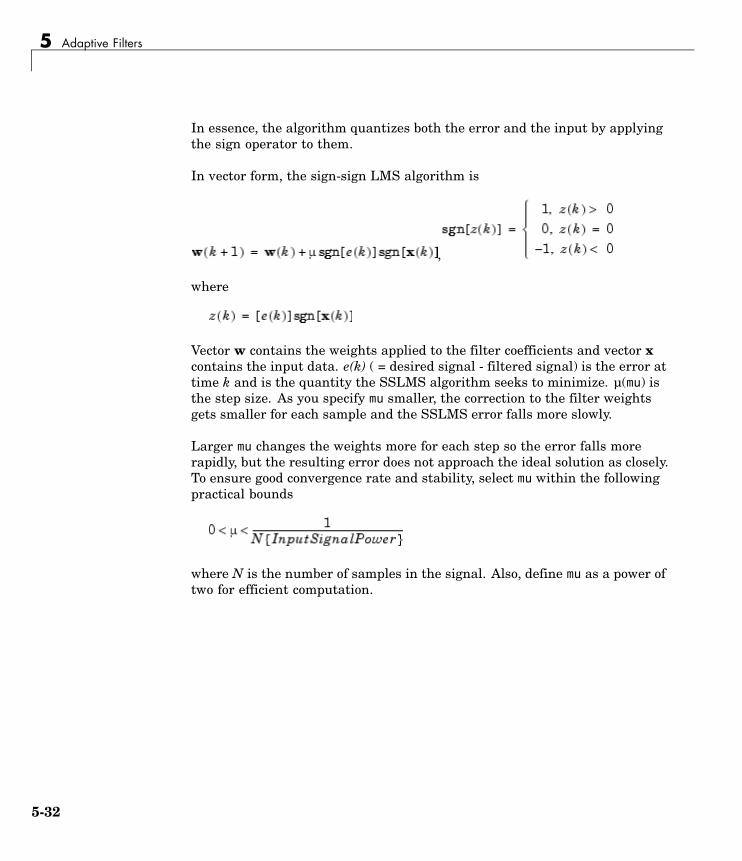
5 Adaptive Filters
In essence, the algorithm quantizes both the error and the input by applyingthe sign operator to them.
In vector form, the sign-sign LMS algorithm is
,
where
Vector w contains the weights applied to the filter coefficients and vector xcontains the input data. e(k) ( = desired signal - filtered signal) is the error attime k and is the quantity the SSLMS algorithm seeks to minimize. µ(mu) isthe step size. As you specify mu smaller, the correction to the filter weightsgets smaller for each sample and the SSLMS error falls more slowly.
Larger mu changes the weights more for each step so the error falls morerapidly, but the resulting error does not approach the ideal solution as closely.To ensure good convergence rate and stability, select mu within the followingpractical bounds
where N is the number of samples in the signal. Also, define mu as a power oftwo for efficient computation.
5-32

Examples of Adaptive Filters That Use LMS Algorithms
Note How you set the initial conditions of the sign-sign algorithm profoundlyinfluences the effectiveness of the adaptation. Because the algorithmessentially quantizes the input signal and the error signal, the algorithmcan become unstable easily.
A series of large error values, coupled with the quantization process mayresult in the error growing beyond all bounds. You restrain the tendency ofthe sign-sign algorithm to get out of control by choosing a small step size (µ<<1) and setting the initial conditions for the algorithm to nonzero positiveand negative values.
In this noise cancellation example, adaptfilt.ss requires two input data sets:
• Data containing a signal corrupted by noise. In Using an Adaptive Filterto Remove Noise from an Unknown System on page 5-9, this is d(k), thedesired signal. The noise cancellation process removes the noise, leavingthe cleaned signal as the content of the error signal.
• Data containing random noise (x(k) in Using an Adaptive Filter to RemoveNoise from an Unknown System on page 5-9) that is correlated with thenoise that corrupts the signal data, called. Without the correlation betweenthe noise data, the adapting algorithm cannot remove the noise from thesignal.
For the signal, use a sine wave. Note that signal is a column vector of 1000elements.
signal = sin(2*pi*0.055*[0:1000-1]');
Now, add correlated white noise to signal. To ensure that the noise iscorrelated, pass the noise through a lowpass FIR filter, then add the filterednoise to the signal.
noise=randn(1,1000);nfilt=fir1(11,0.4); % Eleventh order lowpass filterfnoise=filter(nfilt,1,noise); % Correlated noise datad=signal.'+fnoise;
5-33

5 Adaptive Filters
fnoise is the correlated noise and d is now the desired input to the sign-dataalgorithm.
To prepare the adaptfilt object for processing, set the input conditionscoeffs and mu for the object. As noted earlier in this section, the values you setfor coeffs and mu determine whether the adaptive filter can remove the noisefrom the signal path. In “adaptfilt.lms Example — System Identification” onpage 5-17, you constructed a default filter that sets the filter coefficients tozeros. Usually that approach does not work for the sign-sign algorithm.
The closer you set your initial filter coefficients to the expected values, themore likely it is that the algorithm remains well behaved and converges to afilter solution that removes the noise effectively. For this example, you startwith the coefficients in the filter you used to filter the noise (nfilt), andmodify them slightly so the algorithm has to adapt.
coeffs = nfilt.' -0.01; % Set the filter initial conditions.mu = 0.05; % Set the step size for algorithm updating.
With the required input arguments for adaptfilt.ss prepared, run theadaptation and view the results.
ha = adaptfilt.ss(12,mu)set(ha,'coefficients',coeffs);set(ha,'persistentmemory',true); % Prevent filter reset.[y,e] = filter(ha,noise,d);plot(0:199,signal(1:200),0:199,e(1:200));
Notice that you have to set the property PersistentMemory to true when youmanually change the settings of object ha.
If PersistentMemory is left to false, when you try to apply ha with themethod filter the filtering process starts by resetting the object properties totheir initial conditions at construction. To preserve the customized coefficientsin this example, you set PersistentMemory to true so the coefficients do notget reset automatically back to zero.
When adaptfilt.ss runs, it uses far fewer multiply operations than either ofthe LMS algorithms. Also, performing the sign-sign adaptation requires onlybit shifting multiplies when the step size is a power of two.
5-34

Examples of Adaptive Filters That Use LMS Algorithms
Although the performance of the sign-sign algorithm as shown in the nextfigure is quite good, the sign-sign algorithm is much less stable than thestandard LMS variations. In this noise cancellation example, the signal afterprocessing is a very good match to the input signal, but the algorithm couldvery easily become unstable rather than achieve good performance.
Changing coeffs, mu, or even the lowpass filter you used to create thecorrelated noise can cause noise cancellation to fail and the algorithm tobecome useless.
0 20 40 60 80 100 120 140 160 180 200−2.5
−2
−1.5
−1
−0.5
0
0.5
1
1.5
2
2.5Noise Cancellation Performance of the Sign−Sign LMS Algorithm
Sample Number
Err
or V
alue
Actual SignalError After Noise Reduction
As an aside, the sign-sign LMS algorithm is part of the international CCITTstandard for 32 Kb/s ADPCM telephony.
5-35
5 Adaptive Filters
Example of Adaptive Filter That Uses RLS Algorithm
In this section...
“Introduction and Comparison to the LMS Algorithm” on page 5-36
“adaptfilt.rls Example — Inverse System Identification” on page 5-37
Introduction and Comparison to the LMS AlgorithmThis section provides an introductory example that uses the RLS adaptivefilter function adaptfilt.rls.
If LMS algorithms represent the simplest and most easily applied adaptivealgorithms, the recursive least squares (RLS) algorithms represents increasedcomplexity, computational cost, and fidelity. In performance, RLS approachesthe Kalman filter in adaptive filtering applications, at somewhat reducedrequired throughput in the signal processor.
Compared to the LMS algorithm, the RLS approach offers faster convergenceand smaller error with respect to the unknown system, at the expense ofrequiring more computations.
In contrast to the least mean squares algorithm, from which it can be derived,the RLS adaptive algorithm minimizes the total squared error between thedesired signal and the output from the unknown system.
Referring to , you see the signal flow graph (or model) for the RLS adaptivefilter system. Note that the signal paths and identifications are the samewhether the filter uses RLS or LMS. The difference lies in the adaptingportion.
Within limits, you can use any of the adaptive filter algorithms to solve anadaptive filter problem by replacing the adaptive portion of the applicationwith a new algorithm.
Examples of the sign variants of the LMS algorithms demonstrated thisfeature to demonstrate the differences between the sign-data, sign-error, andsign-sign variations of the LMS algorithm.
5-36

Example of Adaptive Filter That Uses RLS Algorithm
One interesting input option that applies to RLS algorithms is not present inthe LMS processes — a forgetting factor, λ, that determines how the algorithmtreats past data input to the algorithm.
When the LMS algorithm looks at the error to minimize, it considers only thecurrent error value. In the RLS method, the error considered is the total errorfrom the beginning to the current data point.
Said another way, the RLS algorithm has infinite memory — all error data isgiven the same consideration in the total error. In cases where the error valuemight come from a spurious input data point or points, the forgetting factorlets the RLS algorithm reduce the value of older error data by multiplyingthe old data by the forgetting factor.
Since 0 ≤λ< 1, applying the factor is equivalent to weighting the older error.When λ = 1, all previous error is considered of equal weight in the total error.
As λ approaches zero, the past errors play a smaller role in the total. Forexample, when λ = 0.9, the RLS algorithm multiplies an error value from 50samples in the past by an attenuation factor of 0.950 = 5.15 x 10⁻³, considerablydeemphasizing the influence of the past error on the current total error.
adaptfilt.rls Example — Inverse System IdentificationRather than use a system identification application to demonstrate the RLSadaptive algorithm, or a noise cancellation model, this example use theinverse system identification model shown in here.
����
�� ��!���"����
���� �������� �������
����
���� �����
�
5-37

5 Adaptive Filters
Cascading the adaptive filter with the unknown filter causes the adaptivefilter to converge to a solution that is the inverse of the unknown system.
If the transfer function of the unknown is H(z) and the adaptive filtertransfer function is G(z), the error measured between the desired signaland the signal from the cascaded system reaches its minimum when theproduct of H(z) and G(z) is 1, G(z)*H(z) = 1. For this relation to be true,G(z) must equal -H(z), the inverse of the transfer function of the unknownsystem.
To demonstrate that this is true, create a signal to input to the cascadedfilter pair.
x = randn(1,3000);
In the cascaded filters case, the unknown filter results in a delay in the signalarriving at the summation point after both filters. To prevent the adaptivefilter from trying to adapt to a signal it has not yet seen (equivalent topredicting the future), delay the desired signal by 32 samples, the order ofthe unknown system.
Generally, you do not know the order of the system you are trying to identify.In that case, delay the desired signal by the number of samples equal to halfthe order of the adaptive filter. Delaying the input requires prepending 12zero-values samples to x.
delay = zeros(1,12);d = [delay x(1:2988)]; % Concatenate the delay and the signal.
You have to keep the desired signal vector d the same length as x, henceadjust the signal element count to allow for the delay samples.
Although not generally true, for this example you know the order of theunknown filter, so you add a delay equal to the order of the unknown filter.
For the unknown system, use a lowpass, 12th-order FIR filter.
ufilt = fir1(12,0.55,'low');
Filtering x provides the input data signal for the adaptive algorithm function.
5-38

Example of Adaptive Filter That Uses RLS Algorithm
xdata = filter(ufilt,1,x);
To set the input argument values for the adaptfilt.rls object, use theconstructor adaptfilt.rls, providing the needed arguments l, lambda, andinvcov.
For more information about the input conditions to prepare the RLS algorithmobject, refer to adaptfilt.rls in the reference section of this user’s guide.
p0 = 2*eye(13);lambda = 0.99;ha = adaptfilt.rls(13,lambda,p0);
Most of the process to this point is the same as the preceding examples.However, since this example seeks to develop an inverse solution, you need tobe careful about which signal carries the data and which is the desired signal.
Earlier examples of adaptive filters use the filtered noise as the desiredsignal. In this case, the filtered noise (xdata) carries the unknown systeminformation. With Gaussian distribution and variance of 1, the unfilterednoise d is the desired signal. The code to run this adaptive filter example is
[y,e] = filter(ha,xdata,d);
where y returns the coefficients of the adapted filter and e contains the errorsignal as the filter adapts to find the inverse of the unknown system. You canreview the returned elements of the adapted filter in the properties of ha.
The next figure presents the results of the adaptation. In the figure, themagnitude response curves for the unknown and adapted filters show. As areminder, the unknown filter was a lowpass filter with cutoff at 0.55, on thenormalized frequency scale from 0 to 1.
5-39

5 Adaptive Filters
0 0.1 0.2 0.3 0.4 0.5 0.6 0.7 0.8 0.9 1−1200
−1000
−800
−600
−400
−200
0
Normalized Frequency (×π rad/sample)
Pha
se (
degr
ees)
0 0.1 0.2 0.3 0.4 0.5 0.6 0.7 0.8 0.9 1−150
−100
−50
0
50
Normalized Frequency (×π rad/sample)
Mag
nitu
de (
dB)
Comparing the Inverse Filter to the Unknown System
Inverse FilterUnknown System
Viewed alone (refer to the following figure), the inverse system looks like afair compensator for the unknown lowpass filter — a high pass filter withlinear phase.
5-40

Selected Bibliography
0 0.1 0.2 0.3 0.4 0.5 0.6 0.7 0.8 0.9 1−1200
−1000
−800
−600
−400
−200
0
Normalized Frequency (×π rad/sample)
Pha
se (
degr
ees)
0 0.1 0.2 0.3 0.4 0.5 0.6 0.7 0.8 0.9 1−10
0
10
20
30
40
Normalized Frequency (×π rad/sample)
Mag
nitu
de (
dB)
Inverse Filter Resulting from RLS Adaptation
Selected Bibliography[1] Hayes, Monson H., Statistical Digital Signal Processing and Modeling,John Wiley & Sons, 1996, 493–552.
[2] Haykin, Simon, Adaptive Filter Theory, Prentice-Hall, Inc., 1996
5-41

5 Adaptive Filters
5-42

6
Reference for the Propertiesof Filter Objects
Fixed-Point Filter Properties (p. 6-2) Provides an overview and details ofthe properties of fixed-point filters
Adaptive Filter Properties (p. 6-103) Summarizes and details theproperties of adaptive filters
Multirate Filter Properties (p. 6-116) Provides a summary and the detailsof the properties of multirate filters

6 Reference for the Properties of Filter Objects
Fixed-Point Filter Properties
In this section...
“Overview of Fixed-Point Filters” on page 6-2
“Fixed-Point Objects and Filters” on page 6-2
“Summary — Fixed-Point Filter Properties” on page 6-5
“Property Details for Fixed-Point Filters” on page 6-19
Overview of Fixed-Point FiltersThere is a distinction between fixed-point filters and quantized filters —quantized filters represent a superset that includes fixed-point filters.
When dfilt objects have their Arithmetic property set to single or fixed,they are quantized filters. However, after you set the Arithmetic propertyto fixed, the resulting filter is both quantized and fixed-point. Fixed-pointfilters perform arithmetic operations without allowing the binary point tomove in response to the calculation — hence the name fixed-point. Youcan find out more about fixed-point arithmetic in your Fixed-Point Toolboxdocumentation or from the Help system.
With the Arithmetic property set to single, meaning the filter usessingle-precision floating-point arithmetic, the filter allows the binary point tomove during mathematical operations, such as sums or products. Thereforethese filters cannot be considered fixed-point filters. But they are quantizedfilters.
The following sections present the properties for fixed-point filters,which includes all the properties for double-precision and single-precisionfloating-point filters as well.
Fixed-Point Objects and FiltersFixed-point filters depend in part on fixed-point objects from Fixed-PointToolbox. You can see this when you display a fixed-point filter at the commandprompt.
hd=dfilt.df2t
6-2

Fixed-Point Filter Properties
hd =
FilterStructure: 'Direct-Form II Transposed'Arithmetic: 'double'Numerator: 1
Denominator: 1PersistentMemory: false
States: [0x1 double]
set(hd,'arithmetic','fixed')hd
hd =
FilterStructure: 'Direct-Form II Transposed'Arithmetic: 'fixed'Numerator: 1
Denominator: 1PersistentMemory: false
States: [1x1 embedded.fi]
CoeffWordLength: 16CoeffAutoScale: true
Signed: true
InputWordLength: 16InputFracLength: 15
OutputWordLength: 16OutputFracLength: 15
StateWordLength: 16StateAutoScale: true
ProductMode: 'FullPrecision'
AccumWordLength: 40CastBeforeSum: true
6-3

6 Reference for the Properties of Filter Objects
RoundMode: 'convergent'OverflowMode: 'wrap'
Look at the States property, shown here
States: [1x1 embedded.fi]
The notation embedded.fi indicates that the states are being represented byfixed-point objects, usually called fi objects. If you take a closer look at theproperty States, you see how the properties of the fi object represent thevalues for the filter states.
hd.states
ans =
[]
DataType: FixedScaling: BinaryPointSigned: true
WordLength: 16FractionLength: 15
RoundMode: roundOverflowMode: saturateProductMode: FullPrecision
MaxProductWordLength: 128SumMode: FullPrecision
MaxSumWordLength: 128CastBeforeSum: true
To learn more about fi objects (fixed-point objects) in general, refer to yourFixed-Point Toolbox documentation. Commands like the following can helpyou get the information you are looking for:
docsearch(fixed-point object)
or
docsearch(fi)
6-4

Fixed-Point Filter Properties
Either command opens the Help system and searches for information aboutfixed-point objects in Fixed Point Toolbox.
As inputs (data to be filtered), fixed-point filters accept both regulardouble-precision values and fi objects. Which you use depends on your needs.How your filter responds to the input data is determined by the settings of thefilter properties, discussed in the next few sections.
Summary — Fixed-Point Filter PropertiesDiscrete-time filters in this toolbox use objects that perform the filtering andconfiguration of the filter. As objects, they include properties and methodsthat are often referred to as functions — not strictly the same as MATLABfunctions but mostly so) to provide filtering capability. In discrete-time filters,or dfilt objects, many of the properties are dynamic, meaning they becomeavailable depending on the settings of other properties in the dfilt objector filter.
Dynamic PropertiesWhen you use a dfilt.structure function to create a filter, MATLABdisplays the filter properties in the command window in return (unless youend the command with a semicolon which suppresses the output display).Generally you see six or seven properties, ranging from the propertyFilterStructure to PersistentMemory. These first properties are alwayspresent in the filter. One of the most important properties is Arithmetic. TheArithmetic property controls all of the dynamic properties for a filter.
Dynamic properties become available when you change another property inthe filter. For example, when you change the Arithmetic property value tofixed, the display now shows many more properties for the filter, all of themconsidered dynamic. Here is an example that uses a direct form II filter.First create the default filter:
hd=dfilt.df2
hd =
FilterStructure: 'Direct-Form II'Arithmetic: 'double'
6-5
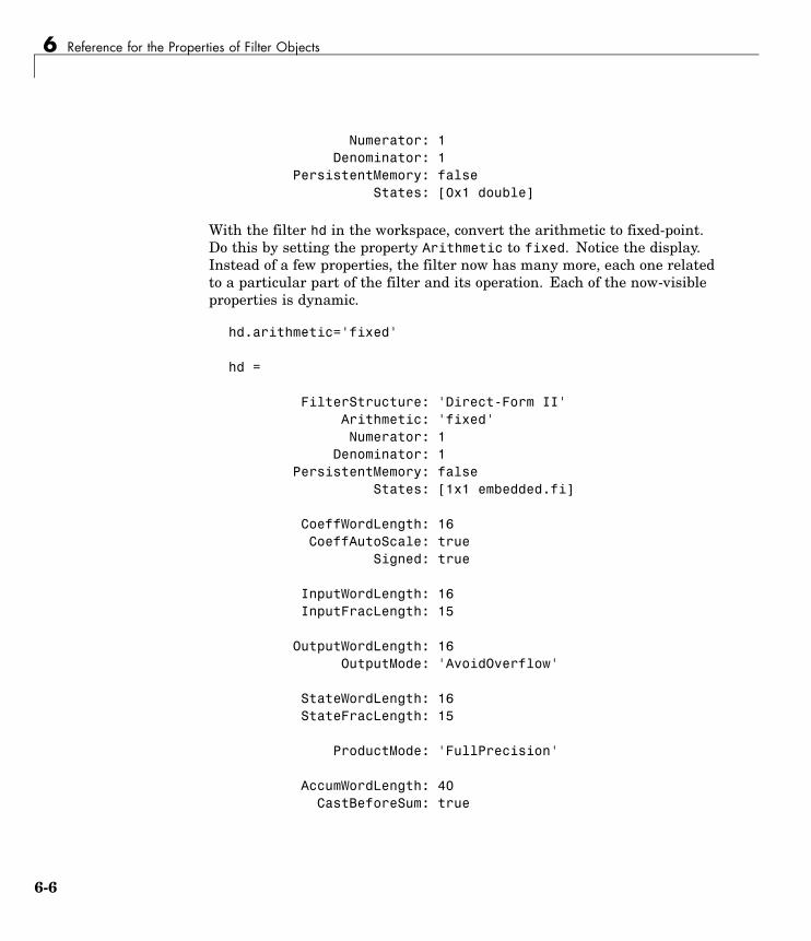
6 Reference for the Properties of Filter Objects
Numerator: 1Denominator: 1
PersistentMemory: falseStates: [0x1 double]
With the filter hd in the workspace, convert the arithmetic to fixed-point.Do this by setting the property Arithmetic to fixed. Notice the display.Instead of a few properties, the filter now has many more, each one relatedto a particular part of the filter and its operation. Each of the now-visibleproperties is dynamic.
hd.arithmetic='fixed'
hd =
FilterStructure: 'Direct-Form II'Arithmetic: 'fixed'Numerator: 1
Denominator: 1PersistentMemory: false
States: [1x1 embedded.fi]
CoeffWordLength: 16CoeffAutoScale: true
Signed: true
InputWordLength: 16InputFracLength: 15
OutputWordLength: 16OutputMode: 'AvoidOverflow'
StateWordLength: 16StateFracLength: 15
ProductMode: 'FullPrecision'
AccumWordLength: 40CastBeforeSum: true
6-6

Fixed-Point Filter Properties
RoundMode: 'convergent'OverflowMode: 'wrap'
Even this list of properties is not yet complete. Changing the value of otherproperties such as the ProductMode or CoeffAutoScale properties mayreveal even more properties that control how the filter works. Remember thisfeature about dfilt objects and dynamic properties as you review the rest ofthis section about properties of fixed-point filters.
An important distinction is you cannot change the value of a property unlessyou see the property listed in the default display for the filter. Entering thefilter name at the MATLAB prompt generates the default property displayfor the named filter. Using get(filtername) does not generate the defaultdisplay — it lists all of the filter properties, both those that you can changeand those that are not available yet.
The following table summarizes the properties, static and dynamic, offixed-point filters and provides a brief description of each. Full descriptions ofeach property, in alphabetical order, follow the table.
Property NameValid Values [DefaultValue] Brief Description
AccumFracLength Any positive or negativeinteger number of bits [29]
Specifies the fraction length usedto interpret data output by theaccumulator. This is a property ofFIR filters and lattice filters. IIRfilters have two similar properties— DenAccumFracLength andNumAccumFracLength — that letyou set the precision for numerator anddenominator operations separately.
AccumWordLength Any positive integer numberof bits [40]
Sets the word length used to store datain the accumulator/buffer.
6-7

6 Reference for the Properties of Filter Objects
Property NameValid Values [DefaultValue] Brief Description
Arithmetic [Double], single, fixed Defines the arithmetic the filter uses.Gives you the options double, single,and fixed. In short, this propertydefines the operating mode for yourfilter.
CastBeforeSum [True] or false Specifies whether to cast numeric datato the appropriate accumulator format(as shown in the signal flow diagrams)before performing sum operations.
CoeffAutoScale [True] or false Specifies whether the filterautomatically chooses the properfraction length to represent filtercoefficients without overflowing.Turning this off by setting the valueto false enables you to change theNumFracLength and DenFracLengthproperties to specify the precision used.
CoeffFracLength Any positive or negativeinteger number of bits [14]
Set the fraction length the filteruses to interpret coefficients.CoeffFracLength is not available untilyou set CoeffAutoScale to false.Scalar filters include this property.
CoeffWordLength Any positive integer numberof bits [16]
Specifies the word length to apply tofilter coefficients.
DenAccumFracLength Any positive or negativeinteger number of bits [29]
Specifies how the filter algorithminterprets the results of additionoperations involving denominatorcoefficients.
DenFracLength Any positive or negativeinteger number of bits [14]
Sets the fraction length the filter usesto interpret denominator coefficients.DenFracLength is always available,but it is read-only until you setCoeffAutoScale to false.
6-8

Fixed-Point Filter Properties
Property NameValid Values [DefaultValue] Brief Description
Denominator Any filter coefficient value[1]
Holds the denominator coefficients forIIR filters.
DenProdFracLength Any positive or negativeinteger number of bits [29]
Specifies how the filter algorithminterprets the results of productoperations involving denominatorcoefficients. You can changethis property value after you setProductMode to SpecifyPrecision.
DenStateFracLength Any positive or negativeinteger number of bits [15]
Specifies the fraction length used tointerpret the states associated withdenominator coefficients in the filter.
FracDelay Any decimal value between0 and 1 samples
Specifies the fractional delay providedby the filter, in decimal fractions of asample.
FDAutoScale [True] or false Specifies whether the filterautomatically chooses the properscaling to represent the fractionaldelay value without overflowing.Turning this off by setting the valueto false enables you to change theFDWordLength and FDFracLengthproperties to specify the data formatapplied.
FDFracLength Any positive or negativeinteger number of bits [5]
Specifies the fraction length torepresent the fractional delay.
FDProdFracLength Any positive or negativeinteger number of bits [34]
Specifies the fraction length torepresent the result of multiplying thecoefficients with the fractional delay.
FDProdWordLength Any positive or negativeinteger number of bits [39]
Specifies the word length to representresult of multiplying the coefficientswith the fractional delay.
FDWordLength Any positive or negativeinteger number of bits [6]
Specifies the word length to representthe fractional delay.
6-9

6 Reference for the Properties of Filter Objects
Property NameValid Values [DefaultValue] Brief Description
DenStateWordLength Any positive integer numberof bits [16]
Specifies the word length used torepresent the states associated withdenominator coefficients in the filter.
FilterInternals [FullPrecision],SpecifyPrecision
Controls whether the filter sets theoutput word and fraction lengths, andthe accumulator word and fractionlengths automatically to maintain thebest precision results during filtering.The default value, FullPrecision,sets automatic word and fractionlength determination by the filter.SpecifyPrecision exposes the outputand accumulator related properties soyou can set your own word and fractionlengths for them.
FilterStructure Not applicable. Describes the signal flow for the filterobject, including all of the activeelements that perform operationsduring filtering — gains, delays, sums,products, and input/output.
InputFracLength Any positive or negativeinteger number of bits [15]
Specifies the fraction length the filteruses to interpret data to be processedby the filter.
InputWordLength Any positive integer numberof bits [16]
Specifies the word length applied torepresent input data.
Ladder Any ladder coefficients indouble-precision data type[1]
latticearma filters include thisproperty to store the ladder coefficients.
LadderAccumFracLength
Any positive or negativeinteger number of bits [29]
latticearma filters use this to definethe fraction length applied to valuesoutput by the accumulator that storesthe results of ladder computations.
6-10
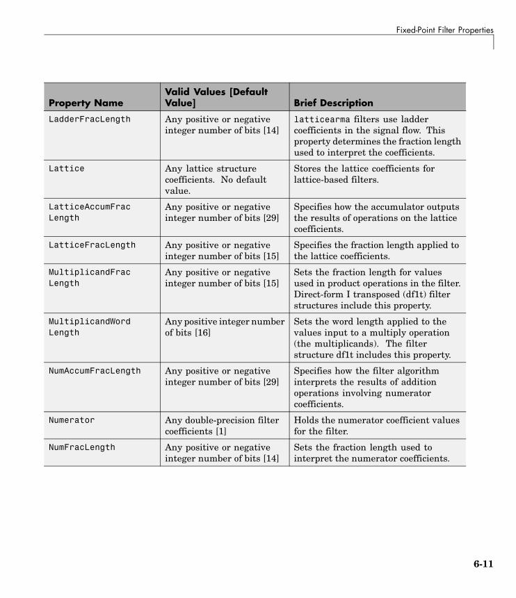
Fixed-Point Filter Properties
Property NameValid Values [DefaultValue] Brief Description
LadderFracLength Any positive or negativeinteger number of bits [14]
latticearma filters use laddercoefficients in the signal flow. Thisproperty determines the fraction lengthused to interpret the coefficients.
Lattice Any lattice structurecoefficients. No defaultvalue.
Stores the lattice coefficients forlattice-based filters.
LatticeAccumFracLength
Any positive or negativeinteger number of bits [29]
Specifies how the accumulator outputsthe results of operations on the latticecoefficients.
LatticeFracLength Any positive or negativeinteger number of bits [15]
Specifies the fraction length applied tothe lattice coefficients.
MultiplicandFracLength
Any positive or negativeinteger number of bits [15]
Sets the fraction length for valuesused in product operations in the filter.Direct-form I transposed (df1t) filterstructures include this property.
MultiplicandWordLength
Any positive integer numberof bits [16]
Sets the word length applied to thevalues input to a multiply operation(the multiplicands). The filterstructure df1t includes this property.
NumAccumFracLength Any positive or negativeinteger number of bits [29]
Specifies how the filter algorithminterprets the results of additionoperations involving numeratorcoefficients.
Numerator Any double-precision filtercoefficients [1]
Holds the numerator coefficient valuesfor the filter.
NumFracLength Any positive or negativeinteger number of bits [14]
Sets the fraction length used tointerpret the numerator coefficients.
6-11

6 Reference for the Properties of Filter Objects
Property NameValid Values [DefaultValue] Brief Description
NumProdFracLength Any positive or negativeinteger number of bits [29]
Specifies how the filter algorithminterprets the results of productoperations involving numeratorcoefficients. You can changethe property value after you setProductMode to SpecifyPrecision.
NumStateFracLength Any positive or negativeinteger number of bits [15]
For IIR filters, this defines the fractionlength applied to the numerator statesof the filter. Specifies the fractionlength used to interpret the statesassociated with numerator coefficientsin the filter.
NumStateWordLength Any positive integer numberof bits [16]
For IIR filters, this defines the wordlength applied to the numerator statesof the filter. Specifies the word lengthused to interpret the states associatedwith numerator coefficients in thefilter.
OutputFracLength Any positive or negativeinteger number of bits —[15] or [12] bits dependingon the filter structure
Determines how the filter interpretsthe filtered data. You can change thevalue of OutputFracLength after youset OutputMode to SpecifyPrecision.
6-12

Fixed-Point Filter Properties
Property NameValid Values [DefaultValue] Brief Description
OutputMode [AvoidOverflow],BestPrecision,SpecifyPrecision
Sets the mode the filter uses to scalethe filtered input data. You have thefollowing choices:
• AvoidOverflow — directs the filterto set the output data fraction lengthto avoid causing the data to overflow.
• BestPrecision — directs the filterto set the output data fraction lengthto maximize the precision in theoutput data.
• SpecifyPrecision — lets you setthe fraction length used by thefiltered data.
OutputWordLength Any positive integer numberof bits [16]
Determines the word length used forthe filtered data.
OverflowMode Saturate or [wrap] Sets the mode used to respond tooverflow conditions in fixed-pointarithmetic. Choose from eithersaturate (limit the output tothe largest positive or negativerepresentable value) or wrap (setoverflowing values to the nearestrepresentable value using modulararithmetic. The choice you makeaffects only the accumulator andoutput arithmetic. Coefficient andinput arithmetic always saturates.Finally, products never overflow — heymaintain full precision.
6-13

6 Reference for the Properties of Filter Objects
Property NameValid Values [DefaultValue] Brief Description
ProductFracLength Any positive or negativeinteger number of bits [29]
For the output from a productoperation, this sets the fraction lengthused to interpret the numeric data.This property becomes writable (youcan change the value) after you setProductMode to SpecifyPrecision.
ProductMode [FullPrecision], KeepLSB,KeepMSB, SpecifyPrecision
Determines how the filter handles theoutput of product operations. Choosefrom full precision (FullPrecision), orwhether to keep the most significantbit (KeepMSB) or least significant bit(KeepLSB) in the result when you needto shorten the data words. For you tobe able to set the precision (the fractionlength) used by the output from themultiplies, you set ProductMode toSpecifyPrecision.
ProductWordLength Any positive number ofbits. Default is 16 or 32depending on the filterstructure
Specifies the word length to use for theresults of multiplication operations.This property becomes writable (youcan change the value) after you setProductMode to SpecifyPrecision.
PersistentMemory True or [false] Specifies whether to reset the filterstates and memory before each filteringoperation. Lets you decide whetheryour filter retains states from previousfiltering runs. True is the defaultsetting.
6-14
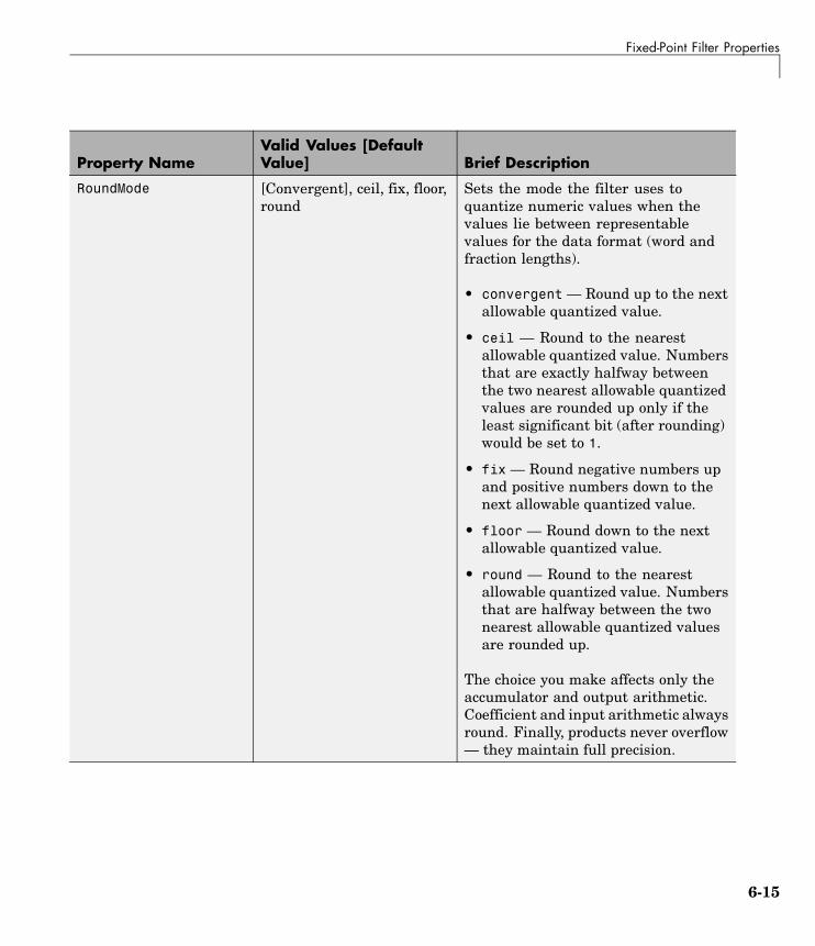
Fixed-Point Filter Properties
Property NameValid Values [DefaultValue] Brief Description
RoundMode [Convergent], ceil, fix, floor,round
Sets the mode the filter uses toquantize numeric values when thevalues lie between representablevalues for the data format (word andfraction lengths).
• convergent — Round up to the nextallowable quantized value.
• ceil — Round to the nearestallowable quantized value. Numbersthat are exactly halfway betweenthe two nearest allowable quantizedvalues are rounded up only if theleast significant bit (after rounding)would be set to 1.
• fix — Round negative numbers upand positive numbers down to thenext allowable quantized value.
• floor — Round down to the nextallowable quantized value.
• round — Round to the nearestallowable quantized value. Numbersthat are halfway between the twonearest allowable quantized valuesare rounded up.
The choice you make affects only theaccumulator and output arithmetic.Coefficient and input arithmetic alwaysround. Finally, products never overflow— they maintain full precision.
6-15

6 Reference for the Properties of Filter Objects
Property NameValid Values [DefaultValue] Brief Description
ScaleValueFracLength Any positive or negativeinteger number of bits [29]
Scale values work with SOS filters.Setting this property controls how yourfilter interprets the scale values bysetting the fraction length. Availableonly when you disable CoeffAutoScaleby setting it to false.
ScaleValues [2 x 1 double] array withvalues of 1
Stores the scaling values for sectionsin SOS filters.
Signed [True] or false Specifies whether the filter uses signedor unsigned fixed-point coefficients.Only coefficients reflect this propertysetting.
sosMatrix [1 0 0 1 0 0] Holds the filter coefficients as propertyvalues. Displays the matrix in theformat [sections x coefficients/sectiondatatype]. A [15x6 double] SOSmatrix represents a filter with 6coefficients per section and 15 sections,using data type double to representthe coefficients.
SectionInputAutoScale
[True] or false Specifies whether the filterautomatically chooses the properfraction length to prevent overflowby data entering a section of anSOS filter. Setting this propertyto false enables you to change theSectionInputFracLength property tospecify the precision used. Availableonly for SOS filters.
6-16

Fixed-Point Filter Properties
Property NameValid Values [DefaultValue] Brief Description
SectionInputFracLength
Any positive or negativeinteger number of bits [29]
Section values work with SOS filters.Setting this property controls howyour filter interprets the sectionvalues between sections of the filterby setting the fraction length. Thisapplies to data entering a section.Compare to SectionOutputFracLength.Available only when you disableSectionInputAutoScale by setting itto false.
SectionInputWordLength
Any positive or negativeinteger number of bits [29]
Sets the word length used to representthe data moving into a section of anSOS filter.
SectionOutputAutoScale
[True] or false Specifies whether the filterautomatically chooses the properfraction length to prevent overflowby data leaving a section of anSOS filter. Setting this propertyto false enables you to change theSectionOutputFracLength property tospecify the precision used.
SectionOutputFracLength
Any positive or negativeinteger number of bits [29]
Section values work with SOS filters.Setting this property controls howyour filter interprets the sectionvalues between sections of the filterby setting the fraction length. Thisapplies to data leaving a section.Compare to SectionInputFracLength.Available after you disableSectionOutputAutoScale by setting itto false.
SectionOutputWordLength
Any positive or negativeinteger number of bits [32]
Sets the word length used to representthe data moving out of one section ofan SOS filter.
6-17

6 Reference for the Properties of Filter Objects
Property NameValid Values [DefaultValue] Brief Description
StateFracLength Any positive or negativeinteger number of bits [15]
Lets you set the fraction length appliedto interpret the filter states.
States [1x1 embedded fi] Contains the filter states before,during, and after filter operations.States act as filter memory betweenfiltering runs or sessions. Noticethat the states use fi objects, withthe associated properties fromthose objects. For details, refer tofiltstates in your Signal ProcessingToolbox documentation or in the Helpsystem.
StateWordLength Any positive integer numberof bits [16]
Sets the word length used to representthe filter states.
TapSumFracLength Any positive or negativeinteger number of bits [15]
Sets the fraction length used torepresent the filter tap values inaddition operations. This is availableafter you set TapSumMode to false.Symmetric and antisymmetric FIRfilters include this property.
6-18

Fixed-Point Filter Properties
Property NameValid Values [DefaultValue] Brief Description
TapSumMode FullPrecision,KeepLSB, [KeepMSB],SpecifyPrecision
Determines how the accumulatoroutputs stored that involve filter tapweights. Choose from full precision(FullPrecision) to prevent overflows,or whether to keep the most significantbits (KeepMSB) or least significantbits (KeepLSB) when outputtingresults from the accumulator. To letyou set the precision (the fractionlength) used by the output from theaccumulator, set FilterInternals toSpecifyPrecision.
Symmetric and antisymmetric FIRfilters include this property.
TapSumWordLength Any positive number of bits[17]
Sets the word length used to representthe filter tap weights during addition.Symmetric and antisymmetric FIRfilters include this property.
Property Details for Fixed-Point FiltersWhen you create a fixed-point filter, you are creating a filter object (a dfiltobject). In this manual, the terms filter, dfilt object, and filter object areused interchangeably. To filter data, you apply the filter object to your dataset. The output of the operation is the data filtered by the filter and the filterproperty values.
Filter objects have properties to which you assign property values. You usethese property values to assign various characteristics to the filters youcreate, including
• The type of arithmetic to use in filtering operations
6-19

6 Reference for the Properties of Filter Objects
• The structure of the filter used to implement the filter (not a property youcan set or change — you select it by the dfilt.structure function youchoose)
• The locations of quantizations and cast operations in the filter
• The data formats used in quantizing, casting, and filtering operations
Details of the properties associated with fixed-point filters are described inalphabetical order on the following pages.
AccumFracLengthExcept for state-space filters, all dfilt objects that use fixed arithmetichave this property that defines the fraction length applied to data in theaccumulator. Combined with AccumWordLength, AccumFracLength helpsfully specify how the accumulator outputs data after processing additionoperations. As with all fraction length properties, AccumFracLength can beany integer, including integers larger than AccumWordLength, and positiveor negative integers.
AccumWordLengthYou use AccumWordLength to define the data word length used in theaccumulator. Set this property to a value that matches your intendedhardware. For example, many digital signal processors use 40-bitaccumulators, so set AccumWordLength to 40 in your fixed-point filter:
set(hq,'arithmetic','fixed');set(hq,'AccumWordLength',40);
Note that AccumWordLength only applies to filters whose Arithmetic propertyvalue is fixed.
ArithmeticPerhaps the most important property when you are working with dfiltobjects, Arithmetic determines the type of arithmetic the filter uses, and theproperties or quantizers that compose the fixed-point or quantized filter. Youuse strings to set the Arithmetic property value.
6-20

Fixed-Point Filter Properties
The next table shows the valid strings for the Arithmetic property. Followingthe table, each property string appears with more detailed information aboutwhat happens when you select the string as the value for Arithmetic inyour dfilt.
ArithmeticPropertyString Brief Description of Effect on the Filter
double All filtering operations and coefficients usedouble-precision floating-point representations andmath. When you use dfilt.structure to create a filterobject, double is the default value for the Arithmeticproperty.
single All filtering operations and coefficients usesingle-precision floating-point representations and math.
fixed This string applies selected default values for theproperties in the fixed-point filter object, includingsuch properties as coefficient word lengths, fractionlengths, and various operating modes. Generally, thedefault values match those you use on many digitalsignal processors. Allows signed fixed data types only.Fixed-point arithmetic filters are available only whenyou install Fixed-Point Toolbox with this toolbox.
double. When you use one of the dfilt.structure methods to create afilter, the Arithmetic property value is double by default. Your filter isidentical to the same filter without the Arithmetic property, as you wouldcreate if you used Signal Processing Toolbox.
Double means that the filter uses double-precision floating-point arithmeticin all operations while filtering:
• All input to the filter must be double data type. Any other data typereturns an error.
• The states and output are doubles as well.
• All internal calculations are done in double math.
6-21
6 Reference for the Properties of Filter Objects
When you use double data type filter coefficients, the reference and quantized(fixed-point) filter coefficients are identical. The filter stores the referencecoefficients as double data type.
single. When your filter should use single-precision floating-point arithmetic,set the Arithmetic property to single so all arithmetic in the filter processinggets restricted to single-precision data type.
• Input data must be single data type. Other data types return errors.
• The filter states and filter output use single data type.
When you choose single, you can provide the filter coefficients in either oftwo ways:
• Double data type coefficients. With Arithmetic set to single, the filtercasts the double data type coefficients to single data type representation.
• Single data type. These remain unchanged by the filter.
Depending on whether you specified single or double data type coefficients,the reference coefficients for the filter are stored in the data type you provided.If you provide coefficients in double data type, the reference coefficients aredouble as well. Providing single data type coefficients generates single datatype reference coefficients. Note that the arithmetic used by the referencefilter is always double.
When you use reffilter to create a reference filter from the referencecoefficients, the resulting filter uses double-precision versions of the referencefilter coefficients.
To set the Arithmetic property value, create your filter, then use set tochange the Arithmetic setting, as shown in this example using a directform FIR filter.
b=fir1(7,0.45);
hd=dfilt.dffir(b)
hd =
6-22

Fixed-Point Filter Properties
FilterStructure: 'Direct-Form FIR'Arithmetic: 'double'Numerator: [1x8 double]
PersistentMemory: falseStates: [7x1 double]
set(hd,'arithmetic','single')hd
hd =
FilterStructure: 'Direct-Form FIR'Arithmetic: 'single'Numerator: [1x8 double]
PersistentMemory: falseStates: [7x1 single]
fixed. Converting your dfilt object to use fixed arithmetic results in a filterstructure that uses properties and property values to match how the filterwould behave on digital signal processing hardware.
Note The fixed option for the property Arithmetic is available only whenyou install Fixed-Point Toolbox as well as Filter Design Toolbox.
After you set Arithmetic to fixed, you are free to change any property valuefrom the default value to a value that more closely matches your needs. Youcannot, however, mix floating-point and fixed-point arithmetic in your filterwhen you select fixed as the Arithmetic property value. Choosing fixedrestricts you to using either fixed-point or floating point throughout the filter(the data type must be homogenous). Also, all data types must be signed.fixed does not support unsigned data types except for unsigned coefficientswhen you set the property Signed to false. Mixing word and fraction lengthswithin the fixed object is acceptable. In short, using fixed arithmetic assumes
• fixed word length.
• fixed size and dedicated accumulator and product registers.
• the ability to do either saturation or wrap arithmetic.
6-23
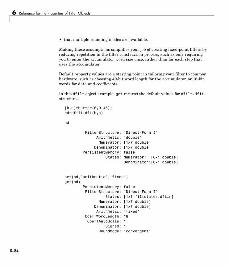
6 Reference for the Properties of Filter Objects
• that multiple rounding modes are available.
Making these assumptions simplifies your job of creating fixed-point filters byreducing repetition in the filter construction process, such as only requiringyou to enter the accumulator word size once, rather than for each step thatuses the accumulator.
Default property values are a starting point in tailoring your filter to commonhardware, such as choosing 40-bit word length for the accumulator, or 16-bitwords for data and coefficients.
In this dfilt object example, get returns the default values for dfilt.df1tstructures.
[b,a]=butter(6,0.45);hd=dfilt.df1(b,a)
hd =
FilterStructure: 'Direct-Form I'Arithmetic: 'double'Numerator: [1x7 double]
Denominator: [1x7 double]PersistentMemory: false
States: Numerator: [6x1 double]Denominator:[6x1 double]
set(hd,'arithmetic','fixed')get(hd)
PersistentMemory: falseFilterStructure: 'Direct-Form I'
States: [1x1 filtstates.dfiir]Numerator: [1x7 double]
Denominator: [1x7 double]Arithmetic: 'fixed'
CoeffWordLength: 16CoeffAutoScale: 1
Signed: 1RoundMode: 'convergent'
6-24

Fixed-Point Filter Properties
OverflowMode: 'wrap'InputWordLength: 16InputFracLength: 15
ProductMode: 'FullPrecision'OutputWordLength: 16OutputFracLength: 15
NumFracLength: 16DenFracLength: 14
ProductWordLength: 32NumProdFracLength: 31DenProdFracLength: 29
AccumWordLength: 40NumAccumFracLength: 31DenAccumFracLength: 29
CastBeforeSum: 1
Here is the default display for hd.
hd
hd =
FilterStructure: 'Direct-Form I'Arithmetic: 'fixed'Numerator: [1x7 double]
Denominator: [1x7 double]PersistentMemory: false
States: Numerator: [6x1 fi]Denominator:[6x1 fi]
CoeffWordLength: 16CoeffAutoScale: true
Signed: true
InputWordLength: 16InputFracLength: 15
OutputWordLength: 16OutputFracLength: 15
6-25

6 Reference for the Properties of Filter Objects
ProductMode: 'FullPrecision'
AccumWordLength: 40CastBeforeSum: true
RoundMode: 'convergent'OverflowMode: 'wrap'
This second example shows the default property values fordfilt.latticemamax filter objects, using the coefficients from an fir1 filter.
b=fir1(7,0.45)
hdlat=dfilt.latticemamax(b)
hdlat =
FilterStructure: [1x45 char]Arithmetic: 'double'
Lattice: [1x8 double]PersistentMemory: false
States: [8x1 double]
hdlat.arithmetic='fixed'
hdlat =
FilterStructure: [1x45 char]Arithmetic: 'fixed'
Lattice: [1x8 double]PersistentMemory: false
States: [1x1 embedded.fi]
CoeffWordLength: 16CoeffAutoScale: true
Signed: true
InputWordLength: 16
6-26

Fixed-Point Filter Properties
InputFracLength: 15
OutputWordLength: 16OutputMode: 'AvoidOverflow'
StateWordLength: 16StateFracLength: 15
ProductMode: 'FullPrecision'
AccumWordLength: 40CastBeforeSum: true
RoundMode: 'convergent'OverflowMode: 'wrap'
Unlike the single or double options for Arithmetic, fixed uses propertiesto define the word and fraction lengths for each portion of your filter. Bychanging the property value of any of the properties, you control your filterperformance. Every word length and fraction length property is independent— set the one you need and the others remain unchanged, such as setting theinput word length with InputWordLength, while leaving the fraction lengththe same.
d=fdesign.lowpass('n,fc',6,0.45)
d =
Response: 'Lowpass with cutoff'Specification: 'N,Fc'
Description: {2x1 cell}NormalizedFrequency: true
Fs: 'Normalized'FilterOrder: 6
Fcutoff: 0.4500
designmethods(d)
6-27

6 Reference for the Properties of Filter Objects
Design Methods for class fdesign.lowpass:
butter
hd=butter(d)
hd =
FilterStructure: 'Direct-Form II, Second-Order Sections'Arithmetic: 'double'sosMatrix: [3x6 double]
ScaleValues: [4x1 double]PersistentMemory: false
States: [2x3 double]
hd.arithmetic='fixed'
hd =
FilterStructure: 'Direct-Form II, Second-Order Sections'Arithmetic: 'fixed'sosMatrix: [3x6 double]
ScaleValues: [4x1 double]PersistentMemory: false
States: [1x1 embedded.fi]
CoeffWordLength: 16CoeffAutoScale: true
Signed: true
InputWordLength: 16InputFracLength: 15
SectionInputWordLength: 16SectionInputAutoScale: true
SectionOutputWordLength: 16Section OutputAutoScale: true
6-28

Fixed-Point Filter Properties
OutputWordLength: 16OutputMode: 'AvoidOverflow'
StateWordLength: 16StateFracLength: 15
ProductMode: 'FullPrecision'
AccumWordLength: 40CastBeforeSum: true
RoundMode: 'convergent'OverflowMode: 'wrap'
hd.inputWordLength=12
hd =
FilterStructure: 'Direct-Form II, Second-Order Sections'Arithmetic: 'fixed'sosMatrix: [3x6 double]
ScaleValues: [4x1 double]PersistentMemory: false
States: [1x1 embedded.fi]
CoeffWordLength: 16CoeffAutoScale: true
Signed: true
InputWordLength: 12InputFracLength: 15
SectionInputWordLength: 16SectionInputAutoScale: true
SectionOutputWordLength: 16SectionOutputAutoScale: true
OutputWordLength: 16OutputMode: 'AvoidOverflow'
6-29

6 Reference for the Properties of Filter Objects
StateWordLength: 16StateFracLength: 15
ProductMode: 'FullPrecision'
AccumWordLength: 40CastBeforeSum: true
RoundMode: 'convergent'OverflowMode: 'wrap'
Notice that the properties for the lattice filter hdlat and direct-form II filter hdare different, as befits their differing filter structures. Also, some propertiesare common to both objects, such as RoundMode and PersistentMemory andbehave the same way in both objects.
Notes About Fraction Length, Word Length, and Precision. Wordlength and fraction length combine to make the format for a fixed-pointnumber, where word length is the number of bits used to represent the valueand fraction length specifies, in bits, the location of the binary point in thefixed-point representation. Therein lies a problem — fraction length, whichyou specify in bits, can be larger than the word length, or a negative numberof bits. This section explains how that idea works and how you might use it.
Unfortunately fraction length is somewhat misnamed (although it continuesto be used in this User’s Guide and elsewhere for historical reasons).
Fraction length defined as the number of fractional bits (bits to the right of thebinary point) is true only when the fraction length is positive and less thanor equal to the word length. In MATLAB format notation you can use [wordlength fraction length]. For example, for the format [16 16], the second 16 (thefraction length) is the number of fractional bits or bits to the right of thebinary point. In this example, all 16 bits are to the right of the binary point.
But it is also possible to have fixed-point formats of [16 18] or [16 -45]. Inthese cases the fraction length can no longer be the number of bits to the rightof the binary point since the format says the word length is 16 — there cannotbe 18 fraction length bits on the right. And how can there be a negativenumber of bits for the fraction length, such as [16 -45]?
6-30

Fixed-Point Filter Properties
A better way to think about fixed-point format [word length fraction length]and what it means is that the representation of a fixed-point number is aweighted sum of powers of two driven by the fraction length, or the two’scomplement representation of the fixed-point number.
Consider the format [B L], where the fraction length L can be positive,negative, 0, greater than B (the word length) or less than B. (B and L arealways integers and B is always positive.)
Given a binary string b(1) b(2) b(3) ... b(B), to determine the two’s-complementvalue of the string in the format described by [B L], use the value of theindividual bits in the binary string in the following formula, where b(1) isthe first binary bit (and most significant bit, MSB), b(2) is the second, andon up to b(B).
The decimal numeric value that those bits represent is given by
value =-b(1)*2^(B-L-1)+b(2)*2^(B-L-2)+b(3)*2^(B-L-3)+...+ b(B)*2^(-L)
L, the fraction length, represents the negative of the weight of the last, orleast significant bit (LSB). L is also the step size or the precision provided bya given fraction length.
Precision. Here is how precision works.
When all of the bits of a binary string are zero except for the LSB (which istherefore equal to one), the value represented by the bit string is given by2(-L). If L is negative, for example L=-16, the value is 216. The smallest stepbetween numbers that can be represented in a format where L=-16 is givenby 1 x 216 (the rightmost term in the formula above), which is 65536. Notethe precision does not depend on the word length.
Take a look at another example. When the word length set to 8 bits, thedecimal value 12 is represented in binary by 00001100. That 12 is thedecimal equivalent of 00001100 tells you that you are using [8 0] data formatrepresentation — the word length is 8 bits and fraction length 0 bits, and thestep size or precision (the smallest difference between two adjacent valuesin the format [8,0], is 20=1.
6-31

6 Reference for the Properties of Filter Objects
Suppose you plan to keep only the upper 5 bits and discard the other three.The resulting precision after removing the right-most three bits comes fromthe weight of the lowest remaining bit, the fifth bit from the left, which is23=8, so the format would be [5,-3].
Note that in this format the step size is 8, I cannot represent numbers thatare between multiples of 8.
In MATLAB, with Fixed-Point Toolbox installed:
x=8;q=quantizer([8,0]); % Word length = 8, fraction length = 0xq=quantize(q,x);binxq=num2bin(q,xq);q1=quantizer([5 -3]); % Word length = 5, fraction length = -3xq1 = quantize(q1,xq);binxq1=num2bin(q1,xq1);binxq
binxq =
00001000
binxq1
binxq1 =
00001
But notice that in [5,-3] format, 00001 is the two’s complement representationfor 8, not for 1; q = quantizer([8 0]) and q1 = quantizer([5 -3]) arenot the same. They cover the about the same range — range(q)>range(q1)— but their quantization step is different — eps(q)= 8, and eps(q1)=1.
Look at one more example. When you construct a quantizer q
q = quantizer([a,b])
the first element in [a,b] is a, the word length used for quantization. Thesecond element in the expression, b, is related to the quantization step —the numerical difference between the two closest values that the quantizer
6-32

Fixed-Point Filter Properties
can represent. This is also related to the weight given to the LSB. Note that2^(-b) = eps(q).
Now construct two quantizers, q1 and q2. Let q1 use the format [32,0] and letq2 use the format [16, -16].
q1 = quantizer([32,0])q2 = quantizer([16,-16])
Quantizers q1 and q2 cover the same range, but q2 has less precision. Itcovers the range in steps of 216, while q covers the range in steps of 1.
This lost precision is due to (or can be used to model) throwing out 16least-significant bits.
An important point to understand is that in dfilt objects and filtering youcontrol which bits are carried from the sum and product operations in thefilter to the filter output by setting the format for the output from the sumor product operation.
For instance, if you use [16 0] as the output format for a 32-bit result from asum operation when the original format is [32 0], you take the lower 16 bitsfrom the result. If you use [16 -16], you take the higher 16 bits of the original32 bits. You could even take 16 bits somewhere in between the 32 bits bychoosing something like [16 -8], but you probably do not want to do that.
Filter scaling is directly implicated in the format and precision for a filter.When you know the filter input and output formats, as well as the filterinternal formats, you can scale the inputs or outputs to stay within the formatranges. For more information about scaling filters, refer to “Converting fromFloating-Point to Fixed-Point”.
Notice that overflows or saturation might occur at the filter input, filteroutput, or within the filter itself, such as during add or multiply or accumulateoperations. Improper scaling at any point in the filter can result in numericalerrors that dramatically change the performance of your fixed-point filterimplementation.
6-33

6 Reference for the Properties of Filter Objects
CastBeforeSumSetting the CastBeforeSum property determines how the filter handlesthe input values to sum operations in the filter. After you set yourfilter Arithmetic property value to fixed, you have the option of usingCastBeforeSum to control the data type of some inputs (addends) tosummations in your filter. To determine which addends reflect theCastBeforeSum property setting, refer to the reference page for the signalflow diagram for the filter structure.
CastBeforeSum specifies whether to cast selected addends to summations inthe filter to the output format from the addition operation before performingthe addition. When you specify true for the property value, the results of theaffected sum operations match most closely the results found on most digitalsignal processors. Performing the cast operation before the summation addsone or two additional quantization operations that can add error sourcesto your filter results.
Specifying CastBeforeSum to be false prevents the addends from being castto the output format before the addition operation. Choose this setting to getthe most accurate results from summations without considering the hardwareyour filter might use.
Notice that the output format for every sum operation reflects the value ofthe output property specified in the filter structure diagram. Which inputproperty is referenced by CastBeforeSum depends on the structure.
Property Value Description
false Configures filter summation operations to retainthe addends in the format carried from the previousoperation.
true Configures filter summation operations to convert theinput format of the addends to match the summationoutput format before performing the summationoperation. Usually this generates results from thesummation that more closely match those found fromdigital signal processors
6-34

Fixed-Point Filter Properties
Another point — with CastBeforeSum set to false, the filter realizationprocess inserts an intermediate data type format to hold temporarily the fullprecision sum of the inputs. A separate Convert block performs the processof casting the addition result to the accumulator format. This intermediatedata format occurs because the Sum block in Simulink always casts input(addends) to the output data type.
Diagrams of CastBeforeSum Settings. When CastBeforeSum is false,sum elements in filter signal flow diagrams look like this:
��##�������
showing that the input data to the sum operations (the addends) retaintheir format word length and fraction length from previous operations. Theaddition process uses the existing input formats and then casts the output tothe format defined by AccumFormat. Thus the output data has the word lengthand fraction length defined by AccumWordLength and AccumFracLength.
When CastBeforeSum is true, sum elements in filter signal flow diagramslook like this:
��##�������
$��
$���##�������
�##�������
6-35
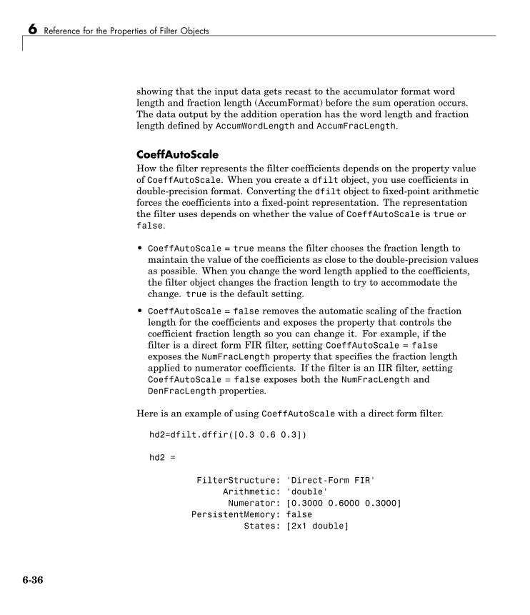
6 Reference for the Properties of Filter Objects
showing that the input data gets recast to the accumulator format wordlength and fraction length (AccumFormat) before the sum operation occurs.The data output by the addition operation has the word length and fractionlength defined by AccumWordLength and AccumFracLength.
CoeffAutoScaleHow the filter represents the filter coefficients depends on the property valueof CoeffAutoScale. When you create a dfilt object, you use coefficients indouble-precision format. Converting the dfilt object to fixed-point arithmeticforces the coefficients into a fixed-point representation. The representationthe filter uses depends on whether the value of CoeffAutoScale is true orfalse.
• CoeffAutoScale = true means the filter chooses the fraction length tomaintain the value of the coefficients as close to the double-precision valuesas possible. When you change the word length applied to the coefficients,the filter object changes the fraction length to try to accommodate thechange. true is the default setting.
• CoeffAutoScale = false removes the automatic scaling of the fractionlength for the coefficients and exposes the property that controls thecoefficient fraction length so you can change it. For example, if thefilter is a direct form FIR filter, setting CoeffAutoScale = falseexposes the NumFracLength property that specifies the fraction lengthapplied to numerator coefficients. If the filter is an IIR filter, settingCoeffAutoScale = false exposes both the NumFracLength andDenFracLength properties.
Here is an example of using CoeffAutoScale with a direct form filter.
hd2=dfilt.dffir([0.3 0.6 0.3])
hd2 =
FilterStructure: 'Direct-Form FIR'Arithmetic: 'double'Numerator: [0.3000 0.6000 0.3000]
PersistentMemory: falseStates: [2x1 double]
6-36

Fixed-Point Filter Properties
hd2.arithmetic='fixed'
hd2 =
FilterStructure: 'Direct-Form FIR'Arithmetic: 'fixed'Numerator: [0.3000 0.6000 0.3000]
PersistentMemory: falseStates: [1x1 embedded.fi]
CoeffWordLength: 16CoeffAutoScale: true
Signed: true
InputWordLength: 16InputFracLength: 15
OutputWordLength: 16OutputMode: 'AvoidOverflow'
ProductMode: 'FullPrecision'
AccumWordLength: 40CastBeforeSum: true
RoundMode: 'convergent'OverflowMode: 'wrap'
To this point, the filter coefficients retain the original values from whenyou created the filter as shown in the Numerator property. Now change theCoeffAutoScale property value from true to false.
hd2.coeffautoScale=false
hd2 =
FilterStructure: 'Direct-Form FIR'Arithmetic: 'fixed'Numerator: [0.3000 0.6000 0.3000]
PersistentMemory: false
6-37

6 Reference for the Properties of Filter Objects
States: [1x1 embedded.fi]
CoeffWordLength: 16CoeffAutoScale: falseNumFracLength: 15
Signed: true
InputWordLength: 16InputFracLength: 15
OutputWordLength: 16OutputMode: 'AvoidOverflow'
ProductMode: 'FullPrecision'
AccumWordLength: 40CastBeforeSum: true
RoundMode: 'convergent'OverflowMode: 'wrap'
With the NumFracLength property now available, change the word lengthto 5 bits.
Notice the coefficient values. Setting CoeffAutoScale to false removes theautomatic fraction length adjustment and the filter coefficients cannot berepresented by the current format of [5 15] — a word length of 5 bits, fractionlength of 15 bits.
hd2.coeffwordlength=5
hd2 =
FilterStructure: 'Direct-Form FIR'Arithmetic: 'fixed'Numerator: [4.5776e-004 4.5776e-004 4.5776e-004]
PersistentMemory: falseStates: [1x1 embedded.fi]
CoeffWordLength: 5
6-38

Fixed-Point Filter Properties
CoeffAutoScale: falseNumFracLength: 15
Signed: true
InputWordLength: 16InputFracLength: 15
OutputWordLength: 16OutputMode: 'AvoidOverflow'
ProductMode: 'FullPrecision'
AccumWordLength: 40CastBeforeSum: true
RoundMode: 'convergent'OverflowMode: 'wrap'
Restoring CoeffAutoScale to true goes some way to fixing the coefficientvalues. Automatically scaling the coefficient fraction length results in settingthe fraction length to 4 bits. You can check this with get(hd2) as shown below.
hd2.coeffautoScale=true
hd2 =
FilterStructure: 'Direct-Form FIR'Arithmetic: 'fixed'Numerator: [0.3125 0.6250 0.3125]
PersistentMemory: falseStates: [1x1 embedded.fi]
CoeffWordLength: 5CoeffAutoScale: true
Signed: true
InputWordLength: 16InputFracLength: 15
OutputWordLength: 16
6-39

6 Reference for the Properties of Filter Objects
OutputMode: 'AvoidOverflow'
ProductMode: 'FullPrecision'
AccumWordLength: 40CastBeforeSum: true
RoundMode: 'convergent'OverflowMode: 'wrap'
get(hd2)PersistentMemory: false
FilterStructure: 'Direct-Form FIR'States: [1x1 embedded.fi]
Numerator: [0.3125 0.6250 0.3125]Arithmetic: 'fixed'
CoeffWordLength: 5CoeffAutoScale: 1
Signed: 1RoundMode: 'convergent'
OverflowMode: 'wrap'InputWordLength: 16InputFracLength: 15
OutputWordLength: 16OutputMode: 'AvoidOverflow'
ProductMode: 'FullPrecision'NumFracLength: 4
OutputFracLength: 12ProductWordLength: 21ProductFracLength: 19
AccumWordLength: 40AccumFracLength: 19
CastBeforeSum: 1
Clearly five bits is not enough to represent the coefficients accurately.
CoeffFracLengthFixed-point scalar filters that you create using dfilt.scalar use thisproperty to define the fraction length applied to the scalar filter coefficients.
6-40

Fixed-Point Filter Properties
Like the coefficient-fraction-length-related properties for the FIR, lattice, andIIR filters, CoeffFracLength is not displayed for scalar filters until you setCoeffAutoScale to false. Once you change the automatic scaling you can setthe fraction length for the coefficients to any value you require.
As with all fraction length properties, the value you enter here can be anynegative or positive integer, or zero. Fraction length can be larger than theassociated word length, as well. By default, the value is 14 bits, with theCoeffWordlength of 16 bits.
CoeffWordLengthOne primary consideration in developing filters for hardware is the lengthof a data word. CoeffWordLength defines the word length for these datastorage and arithmetic locations:
• Numerator and denominator filter coefficients
• Tap sum in dfilt.dfsymfir and dfilt.dfasymfir filter objects
• Section input, multiplicand, and state values in direct-form SOS filterobjects such as dfilt.df1t and dfilt.df2
• Scale values in second-order filters
• Lattice and ladder coefficients in lattice filter objects, such asdfilt.latticearma and dfilt.latticemamax
• Gain in dfilt.scalar
Setting this property value controls the word length for the data listed. Inmost cases, the data words in this list have separate fraction length propertiesto define the associated fraction lengths.
Any positive, integer word length works here, limited by the machine you useto develop your filter and the hardware you use to deploy your filter.
DenAccumFracLengthFilter structures df1, df1t, df2, and df2t that use fixed arithmetic have thisproperty that defines the fraction length applied to denominator coefficientsin the accumulator. In combination with AccumWordLength, the propertiesfully specify how the accumulator outputs data stored there.
6-41

6 Reference for the Properties of Filter Objects
As with all fraction length properties, DenAccumFracLength can be anyinteger, including integers larger than AccumWordLength, and positive ornegative integers. To be able to change the property value for this property,you set FilterInternals to SpecifyPrecision.
DenFracLengthProperty DenFracLength contains the value that specifies the fraction lengthfor the denominator coefficients for your filter. DenFracLength specifies thefraction length used to interpret the data stored in C. Used in combinationwith CoeffWordLength, these two properties define the interpretation of thecoefficients stored in the vector that contains the denominator coefficients.
As with all fraction length properties, the value you enter here can be anynegative or positive integer, or zero. Fraction length can be larger than theassociated word length, as well. By default, the value is 15 bits, with theCoeffWordLength of 16 bits.
DenominatorThe denominator coefficients for your IIR filter, taken from the prototype youstart with, are stored in this property. Generally this is a 1-by-N array of datain double format, where N is the length of the filter.
All IIR filter objects include Denominator, except the lattice-based filterswhich store their coefficients in the Lattice property, and second-ordersection filters, such as dfilt.df1tsos, which use the SosMatrix property tohold the coefficients for the sections.
DenProdFracLengthA property of all of the direct form IIR dfilt objects, except the ones thatimplement second-order sections, DenProdFracLength specifies the fractionlength applied to data output from product operations that the filter performson denominator coefficients.
Looking at the signal flow diagram for the dfilt.df1t filter, for example, yousee that denominators and numerators are handled separately. When you setProductMode to SpecifyPrecision, you can change the DenProdFracLengthsetting manually. Otherwise, for multiplication operations that use the
6-42

Fixed-Point Filter Properties
denominator coefficients, the filter sets the fraction length as defined by theProductMode setting.
DenStateFracLengthWhen you look at the flow diagram for the dfilt.df1sos filter object, thestates associated with denominator coefficient operations take the fractionlength from this property. In combination with the DenStateWordLengthproperty, these properties fully specify how the filter interprets the states.
As with all fraction length properties, the value you enter here can be anynegative or positive integer, or zero. Fraction length can be larger than theassociated word length, as well. By default, the value is 15 bits, with theDenStateWordLength of 16 bits.
DenStateWordLengthWhen you look at the flow diagram for the dfilt.df1sos filter object, thestates associated with the denominator coefficient operations take thedata format from this property and the DenStateFracLength property. Incombination, these properties fully specify how the filter interprets the stateit uses.
By default, the value is 16 bits, with the DenStateFracLength of 15 bits.
FilterInternalsSimilar to the FilterInternals pane in FDATool, this property controls whetherthe filter sets the output word and fraction lengths automatically, and theaccumulator word and fraction lengths automatically as well, to maintain thebest precision results during filtering. The default value, FullPrecision,sets automatic word and fraction length determination by the filter. SettingFilterInternals to SpecifyPrecision exposes the output and accumulatorrelated properties so you can set your own word and fraction lengths forthem. Note that
FilterStructureEvery dfilt object has a FilterStructure property. This is a read-onlyproperty containing a string that declares the structure of the filter objectyou created.
6-43

6 Reference for the Properties of Filter Objects
When you construct filter objects, the FilterStructure property value isreturned containing one of the strings shown in the following table. PropertyFilterStructure indicates the filter architecture and comes from theconstructor you use to create the filter.
After you create a filter object, you cannot change the FilterStructureproperty value. To make filters that use different structures, you constructnew filters using the appropriate methods, or use convert to switch to anew structure.
Default value. Since this depends on the constructor you use and theconstructor includes the filter structure definition, there is no default value.When you try to create a filter without specifying a structure, MATLABreturns an error.
Filter Constructor NameFilterStructure Property String and FilterType
'dfilt.df1' Direct form I
'dfilt.df1sos' Direct form I filter implemented usingsecond-order sections
'dfilt.df1t' Direct form I transposed
'dfilt.df2' Direct form II
'dfilt.df2sos' Direct form II filter implemented using secondorder sections
'dfilt.df2t' Direct form II transposed
'dfilt.dfasymfir' Antisymmetric finite impulse response (FIR).Even and odd forms.
'dfilt.dffir' Direct form FIR
'dfilt.dffirt' Direct form FIR transposed
'dfilt.latticeallpass' Lattice allpass
'dfilt.latticear' Lattice autoregressive (AR)
'dfilt.latticemamin' Lattice moving average (MA) minimum phase
'dfilt.latticemamax' Lattice moving average (MA) maximum phase
6-44

Fixed-Point Filter Properties
Filter Constructor NameFilterStructure Property String and FilterType
'dfilt.latticearma' Lattice ARMA
'dfilt.dfsymfir' Symmetric FIR. Even and odd forms
'dfilt.scalar' Scalar
Filter Structures with Quantizations Shown in Place. To help youunderstand how and where the quantizations occur in filter structures inthis toolbox, the figure below shows the structure for a Direct Form II filter,including the quantizations (fixed-point formats) that compose part of thefixed-point filter. You see that one or more quantization processes, specifiedby the *format label, accompany each filter element, such as a delay, product,or summation element. The input to or output from each element reflects theresult of applying the associated quantization as defined by the word lengthand fraction length format. Wherever a particular filter element appears in afilter structure, recall the quantization process that accompanies the elementas it appears in this figure. Each filter reference page, such as the dfilt.df2reference page, includes the signal flow diagram showing the formattingelements that define the quantizations that occur throughout the filter flow.
For example, a product quantization, either numerator or denominator,follows every product (gain) element and a sum quantization, also eithernumerator or denominator, follows each sum element. The figure shows theArithmetic property value set to fixed.
df2 IIR Filter Structure Including the Formatting Objects, with ArithmeticProperty Value fixed
6-45

6 Reference for the Properties of Filter Objects
When your df2 filter uses the Arithmetic property set to fixed, the filterstructure contains the formatting features shown in the diagram. The formatsincluded in the structure are fixed-point objects that include properties to setvarious word and fraction length formats. For example, the NumFormat orDenFormat in the fixed-point arithmetic filter set the properties for quantizingnumerator or denominator coefficients according to word and fraction lengthsettings.
When the leading denominator coefficient a(1) in your filter is not 1, choose itto be a power of two so that a shift replaces the multiply that would otherwisebe used.
Fixed-Point Arithmetic Filter Structures. You choose among several filterstructures when you create fixed-point filters. You can also specify filters withsingle or multiple cascaded sections of the same type. Because quantization isa nonlinear process, different fixed-point filter structures produce differentresults.
To specify the filter structure, you select the appropriate dfilt.structuremethod to construct your filter. Refer to the function reference information fordfilt and set for details on setting property values for quantized filters.
6-46
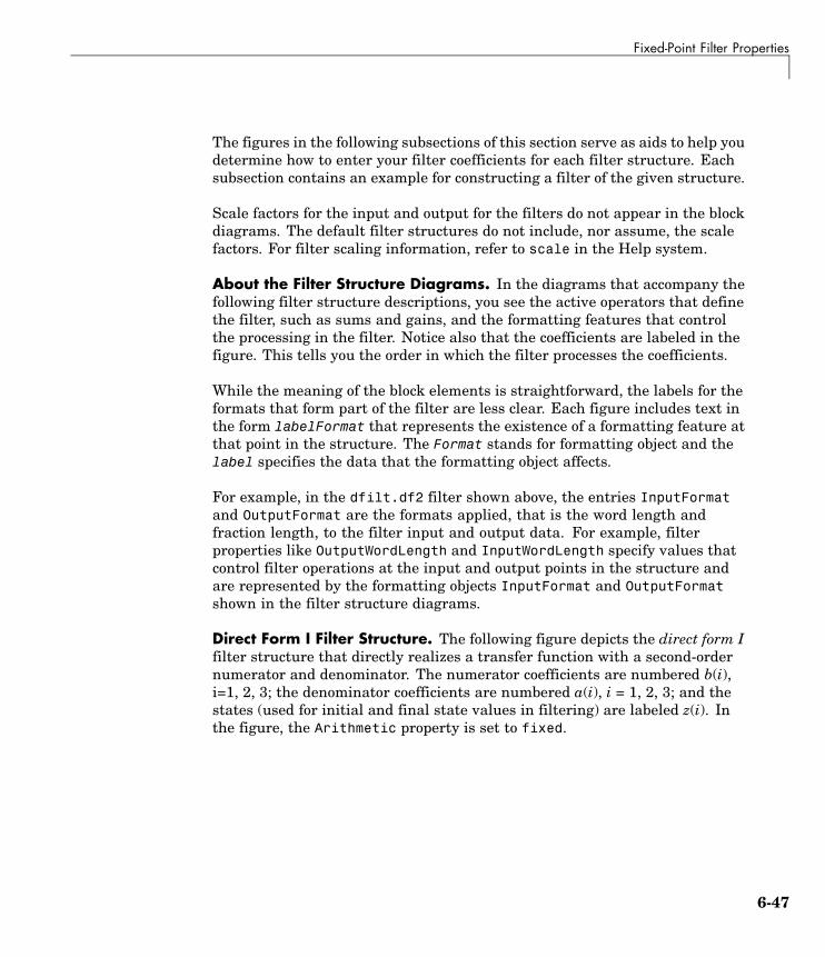
Fixed-Point Filter Properties
The figures in the following subsections of this section serve as aids to help youdetermine how to enter your filter coefficients for each filter structure. Eachsubsection contains an example for constructing a filter of the given structure.
Scale factors for the input and output for the filters do not appear in the blockdiagrams. The default filter structures do not include, nor assume, the scalefactors. For filter scaling information, refer to scale in the Help system.
About the Filter Structure Diagrams. In the diagrams that accompany thefollowing filter structure descriptions, you see the active operators that definethe filter, such as sums and gains, and the formatting features that controlthe processing in the filter. Notice also that the coefficients are labeled in thefigure. This tells you the order in which the filter processes the coefficients.
While the meaning of the block elements is straightforward, the labels for theformats that form part of the filter are less clear. Each figure includes text inthe form labelFormat that represents the existence of a formatting feature atthat point in the structure. The Format stands for formatting object and thelabel specifies the data that the formatting object affects.
For example, in the dfilt.df2 filter shown above, the entries InputFormatand OutputFormat are the formats applied, that is the word length andfraction length, to the filter input and output data. For example, filterproperties like OutputWordLength and InputWordLength specify values thatcontrol filter operations at the input and output points in the structure andare represented by the formatting objects InputFormat and OutputFormatshown in the filter structure diagrams.
Direct Form I Filter Structure. The following figure depicts the direct form Ifilter structure that directly realizes a transfer function with a second-ordernumerator and denominator. The numerator coefficients are numbered b(i),i=1, 2, 3; the denominator coefficients are numbered a(i), i = 1, 2, 3; and thestates (used for initial and final state values in filtering) are labeled z(i). Inthe figure, the Arithmetic property is set to fixed.
6-47

6 Reference for the Properties of Filter Objects
Example — Specifying a Direct Form I Filter. You can specify asecond-order direct form I structure for a quantized filter hq with thefollowing code.
b = [0.3 0.6 0.3];a = [1 0 0.2];hq = dfilt.df1(b,a);
To create the fixed-point filter, set the Arithmetic property to fixed asshown here.
set(hq,'arithmetic','fixed');
Direct Form I Filter Structure With Second-Order Sections. Thefollowing figure depicts a direct form I filter structure that directly realizesa transfer function with a second-order numerator and denominator andsecond-order sections. The numerator coefficients are numbered b(i), i=1, 2, 3;the denominator coefficients are numbered a(i), i = 1, 2, 3; and the states (usedfor initial and final state values in filtering) are labeled z(i). In the figure, theArithmetic property is set to fixed to place the filter in fixed-point mode.
6-48

Fixed-Point Filter Properties
Example — Specifying a Direct Form I Filter with Second-OrderSections. You can specify an eighth-order direct form I structure for aquantized filter hq with the following code.
b = [0.3 0.6 0.3];a = [1 0 0.2];hq = dfilt.df1sos(b,a);
To create the fixed-point filter, set the Arithmetic property to fixed, asshown here.
set(hq,'arithmetic','fixed');
Direct Form I Transposed Filter Structure. The next signal flow diagramdepicts a direct form I transposed filter structure that directly realizes atransfer function with a second-order numerator and denominator. Thenumerator coefficients are b(i), i = 1, 2, 3; the denominator coefficients area(i), i = 1, 2, 3; and the states (used for initial and final state values infiltering) are labeled z(i). With the Arithmetic property value set to fixed,the figure shows the filter with the properties indicated.
6-49
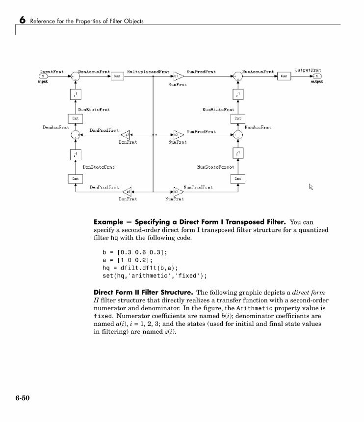
6 Reference for the Properties of Filter Objects
Example — Specifying a Direct Form I Transposed Filter. You canspecify a second-order direct form I transposed filter structure for a quantizedfilter hq with the following code.
b = [0.3 0.6 0.3];a = [1 0 0.2];hq = dfilt.df1t(b,a);set(hq,'arithmetic','fixed');
Direct Form II Filter Structure. The following graphic depicts a direct formII filter structure that directly realizes a transfer function with a second-ordernumerator and denominator. In the figure, the Arithmetic property value isfixed. Numerator coefficients are named b(i); denominator coefficients arenamed a(i), i = 1, 2, 3; and the states (used for initial and final state valuesin filtering) are named z(i).
6-50
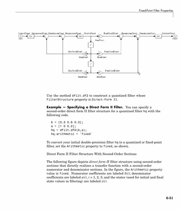
Fixed-Point Filter Properties
Use the method dfilt.df2 to construct a quantized filter whoseFilterStructure property is Direct-Form II.
Example — Specifying a Direct Form II Filter. You can specify asecond-order direct form II filter structure for a quantized filter hq with thefollowing code.
b = [0.3 0.6 0.3];a = [1 0 0.2];hq = dfilt.df2(b,a);hq.arithmetic = 'fixed'
To convert your initial double-precision filter hq to a quantized or fixed-pointfilter, set the Arithmetic property to fixed, as shown.
Direct Form II Filter Structure With Second-Order Sections
The following figure depicts direct form II filter structure using second-ordersections that directly realizes a transfer function with a second-ordernumerator and denominator sections. In the figure, the Arithmetic propertyvalue is fixed. Numerator coefficients are labeled b(i); denominatorcoefficients are labeled a(i), i = 1, 2, 3; and the states (used for initial and finalstate values in filtering) are labeled z(i).
6-51

6 Reference for the Properties of Filter Objects
Use the method dfilt.df2sos to construct a quantized filter whoseFilterStructure property is Direct-Form II.
Example — Specifying a Direct Form II Filter with Second-OrderSections. You can specify a tenth-order direct form II filter structure thatuses second-order sections for a quantized filter hq with the following code.
b = [0.3 0.6 0.3];a = [1 0 0.2];hq = dfilt.df2sos(b,a);hq.arithmetic = 'fixed'
To convert your prototype double-precision filter hq to a fixed-point filter, setthe Arithmetic property to fixed, as shown.
Direct Form II Transposed Filter Structure. The following figure depictsthe direct form II transposed filter structure that directly realizes transferfunctions with a second-order numerator and denominator. The numeratorcoefficients are labeled b(i), the denominator coefficients are labeled a(i), i =1, 2, 3, and the states (used for initial and final state values in filtering) arelabeled z(i). In the first figure, the Arithmetic property value is fixed.
6-52

Fixed-Point Filter Properties
Use the constructor dfilt.df2t to specify the value of the FilterStructureproperty for a filter with this structure that you can convert to fixed-pointfiltering.
Example — Specifying a Direct Form II Transposed Filter. Specifying orconstructing a second-order direct form II transposed filter for a fixed-pointfilter hq starts with the following code to define the coefficients and constructthe filter.
b = [0.3 0.6 0.3];a = [1 0 0.2];hd = dfilt.df2t(b,a);
Now create the fixed-point filtering version of the filter from hd, which isfloating point.
hq = set(hd,'arithmetic','fixed');
6-53
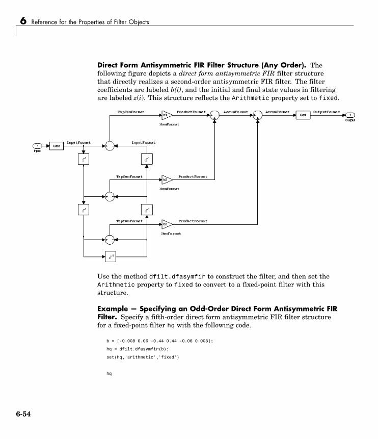
6 Reference for the Properties of Filter Objects
Direct Form Antisymmetric FIR Filter Structure (Any Order). Thefollowing figure depicts a direct form antisymmetric FIR filter structurethat directly realizes a second-order antisymmetric FIR filter. The filtercoefficients are labeled b(i), and the initial and final state values in filteringare labeled z(i). This structure reflects the Arithmetic property set to fixed.
Use the method dfilt.dfasymfir to construct the filter, and then set theArithmetic property to fixed to convert to a fixed-point filter with thisstructure.
Example — Specifying an Odd-Order Direct Form Antisymmetric FIRFilter. Specify a fifth-order direct form antisymmetric FIR filter structurefor a fixed-point filter hq with the following code.
b = [-0.008 0.06 -0.44 0.44 -0.06 0.008];
hq = dfilt.dfasymfir(b);
set(hq,'arithmetic','fixed')
hq
6-54

Fixed-Point Filter Properties
hq =
FilterStructure: 'Direct-Form Antisymmetric FIR'
Arithmetic: 'fixed'
Numerator: [-0.0080 0.0600 -0.4400 0.4400 -0.0600 0.0080]
PersistentMemory: false
States: [1x1 fi object]
CoeffWordLength: 16
CoeffAutoScale: true
Signed: true
InputWordLength: 16
InputFracLength: 15
OutputWordLength: 16
OutputMode: 'AvoidOverflow'
TapSumMode: 'KeepMSB'
TapSumWordLength: 17
ProductMode: 'FullPrecision'
AccumWordLength: 40
CastBeforeSum: true
RoundMode: 'convergent'
OverflowMode: 'wrap'
InheritSettings: false
Example — Specifying an Even-Order Direct Form Antisymmetric FIRFilter. You can specify a fourth-order direct form antisymmetric FIR filterstructure for a fixed-point filter hq with the following code.
b = [-0.01 0.1 0.0 -0.1 0.01];hq = dfilt.dfasymfir(b);hq.arithmetic='fixed'
hq =
6-55

6 Reference for the Properties of Filter Objects
FilterStructure: 'Direct-Form Antisymmetric FIR'Arithmetic: 'fixed'Numerator: [-0.0100 0.1000 0 -0.1000 0.0100]
PersistentMemory: falseStates: [1x1 fi object]
CoeffWordLength: 16CoeffAutoScale: true
Signed: true
InputWordLength: 16InputFracLength: 15
OutputWordLength: 16OutputMode: 'AvoidOverflow'
TapSumMode: 'KeepMSB'TapSumWordLength: 17
ProductMode: 'FullPrecision'
AccumWordLength: 40
CastBeforeSum: trueRoundMode: 'convergent'
OverflowMode: 'wrap'
InheritSettings: false
Direct Form Finite Impulse Response (FIR) Filter Structure. In the nextfigure, you see the signal flow graph for a direct form finite impulse response(FIR) filter structure that directly realizes a second-order FIR filter. Thefilter coefficients are b(i), i = 1, 2, 3, and the states (used for initial and finalstate values in filtering) are z(i). To generate the figure, set the Arithmeticproperty to fixed after you create your prototype filter in double-precisionarithmetic.
6-56

Fixed-Point Filter Properties
Use the dfilt.dffir method to generate a filter that uses this structure.
Example — Specifying a Direct Form FIR Filter. You can specify asecond-order direct form FIR filter structure for a fixed-point filter hq withthe following code.
b = [0.05 0.9 0.05];hd = dfilt.dffir(b);hq = set(hd,'arithmetic','fixed');
Direct Form FIR Transposed Filter Structure. This figure uses the filtercoefficients labeled b(i), i = 1, 2, 3, and states (used for initial and final statevalues in filtering) are labeled z(i). These depict a direct form finite impulseresponse (FIR) transposed filter structure that directly realizes a second-orderFIR filter.
6-57

6 Reference for the Properties of Filter Objects
With the Arithmetic property set to fixed, your filter matches the figure.Using the method dfilt.dffirt returns a double-precision filter that youconvert to a fixed-point filter.
6-58

Fixed-Point Filter Properties
Example — Specifying a Direct Form FIR Transposed Filter. Youcan specify a second-order direct form FIR transposed filter structure for afixed-point filter hq with the following code.
b = [0.05 0.9 0.05];hd=dfilt.dffirt(b);hq = copy(hd);hq.arithmetic = 'fixed';
Lattice Allpass Filter Structure. The following figure depicts the latticeallpass filter structure. The pictured structure directly realizes third-orderlattice allpass filters using fixed-point arithmetic. The filter reflectioncoefficients are labeled k1(i), i = 1, 2, 3. The states (used for initial and finalstate values in filtering) are labeled z(i).
To create a quantized filter that uses the lattice allpass structure shown inthe figure, use the dfilt.latticeallpass method and set the Arithmeticproperty to fixed.
Example — Specifying a Lattice Allpass Filter. You can create athird-order lattice allpass filter structure for a quantized filter hq with thefollowing code.
k = [.66 .7 .44];hd=dfilt.latticeallpass(k);set(hq,'arithmetic','fixed');
6-59
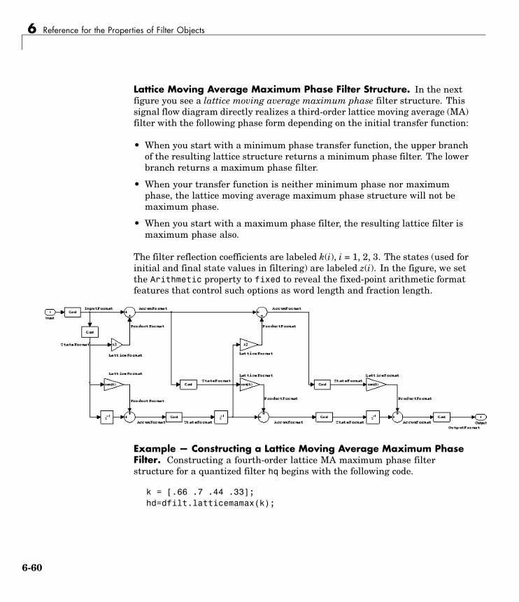
6 Reference for the Properties of Filter Objects
Lattice Moving Average Maximum Phase Filter Structure. In the nextfigure you see a lattice moving average maximum phase filter structure. Thissignal flow diagram directly realizes a third-order lattice moving average (MA)filter with the following phase form depending on the initial transfer function:
• When you start with a minimum phase transfer function, the upper branchof the resulting lattice structure returns a minimum phase filter. The lowerbranch returns a maximum phase filter.
• When your transfer function is neither minimum phase nor maximumphase, the lattice moving average maximum phase structure will not bemaximum phase.
• When you start with a maximum phase filter, the resulting lattice filter ismaximum phase also.
The filter reflection coefficients are labeled k(i), i = 1, 2, 3. The states (used forinitial and final state values in filtering) are labeled z(i). In the figure, we setthe Arithmetic property to fixed to reveal the fixed-point arithmetic formatfeatures that control such options as word length and fraction length.
Example — Constructing a Lattice Moving Average Maximum PhaseFilter. Constructing a fourth-order lattice MA maximum phase filterstructure for a quantized filter hq begins with the following code.
k = [.66 .7 .44 .33];hd=dfilt.latticemamax(k);
6-60

Fixed-Point Filter Properties
Lattice Autoregressive (AR) Filter Structure. The methoddfilt.latticear directly realizes lattice autoregressive filters in the toolbox.The following figure depicts the third-order lattice autoregressive (AR)filter structure — with the Arithmetic property equal to fixed. The filterreflection coefficients are labeled k(i), i = 1, 2, 3, and the states (used forinitial and final state values in filtering) are labeled z(i).
Example — Specifying a Lattice AR Filter. You can specify a third-orderlattice AR filter structure for a quantized filter hq with the following code.
k = [.66 .7 .44];hd=dfilt.latticear(k);hq.arithmetic = 'custom';
Lattice Moving Average (MA) Filter Structure for Minimum Phase.The following figures depict lattice moving average (MA) filter structuresthat directly realize third-order lattice MA filters for minimum phase. Thefilter reflection coefficients are labeled k(i), i = 1, 2, 3, and the states (usedfor initial and final state values in filtering) are labeled z(i). Setting theArithmetic property of the filter to fixed results in a fixed-point filter thatmatches the figure.
This signal flow diagram directly realizes a third-order lattice moving average(MA) filter with the following phase form depending on the initial transferfunction:
6-61

6 Reference for the Properties of Filter Objects
• When you start with a minimum phase transfer function, the upper branchof the resulting lattice structure returns a minimum phase filter. The lowerbranch returns a minimum phase filter.
• When your transfer function is neither minimum phase nor maximumphase, the lattice moving average minimum phase structure will not beminimum phase.
• When you start with a minimum phase filter, the resulting lattice filter isminimum phase also.
The filter reflection coefficients are labeled k(i), i = 1, 2, 3. The states (usedfor initial and final state values in filtering) are labeled z(i). This figure showsthe filter structure when theArithmetic property is set to fixed to revealthe fixed-point arithmetic format features that control such options as wordlength and fraction length.
Example — Specifying a Minimum Phase Lattice MA Filter. Youcan specify a third-order lattice MA filter structure for minimum phaseapplications using variations of the following code.
k = [.66 .7 .44];hd=dfilt.latticemamin(k);set(hq,'arithmetic','fixed');
6-62

Fixed-Point Filter Properties
Lattice Autoregressive Moving Average (ARMA) Filter Structure. Thefigure below depicts a lattice autoregressive moving average (ARMA) filterstructure that directly realizes a fourth-order lattice ARMA filter. The filterreflection coefficients are labeled k(i), i = 1, ..., 4; the ladder coefficients arelabeled v(i), i = 1, 2, 3; and the states (used for initial and final state valuesin filtering) are labeled z(i).
Example — Specifying an Lattice ARMA Filter. The following codespecifies a fourth-order lattice ARMA filter structure for a quantized filter hq,starting from hd, a floating-point version of the filter.
k = [.66 .7 .44 .66];v = [1 0 0];hd=dfilt.latticearma(k,v);hq.arithmetic = 'fixed';
6-63

6 Reference for the Properties of Filter Objects
Direct Form Symmetric FIR Filter Structure (Any Order). Shown in thenext figure, you see signal flow that depicts a direct form symmetric FIR filterstructure that directly realizes a fifth-order direct form symmetric FIR filter.Filter coefficients are labeled b(i),i = 1, ...,n, and states (used for initial andfinal state values in filtering) are labeled z(i). Showing the filter structureused when you select fixed for the Arithmetic property value, the first figuredetails the properties in the filter object.
Example — Specifying an Odd-Order Direct Form Symmetric FIRFilter. By using the following code in MATLAB, you can specify a fifth-orderdirect form symmetric FIR filter for a fixed-point filter hq:
b = [-0.008 0.06 0.44 0.44 0.06 -0.008];hd=dfilt.dfsymfir(b);set(hq,'arithmetic','fixed');
Assigning Filter Coefficients. The syntax you use to assign filter coefficientsfor your floating-point or fixed-point filter depends on the structure youselect for your filter.
6-64

Fixed-Point Filter Properties
Converting Filters Between Representations. Filter conversion functionsin this toolbox and in Signal Processing Toolbox let you convert filter transferfunctions to other filter forms, and from other filter forms to transfer functionform. Relevant conversion functions include the following functions.
ConversionFunction Description
ca2tf Converts from a coupled allpass filter to a transferfunction.
cl2tf Converts from a lattice coupled allpass filter to atransfer function.
convert Convert a discrete-time filter from one filterstructure to another.
sos Converts quantized filters to create second-ordersections. We recommend this method for convertingquantized filters to second-order sections.
tf2ca Converts from a transfer function to a coupledallpass filter.
tf2cl Converts from a transfer function to a lattice coupledallpass filter.
tf2latc Converts from a transfer function to a lattice filter.
tf2sos Converts from a transfer function to a second-ordersection form.
tf2ss Converts from a transfer function to state-spaceform.
tf2zp Converts from a rational transfer function to itsfactored (single section) form (zero-pole-gain form).
zp2sos Converts a zero-pole-gain form to a second-ordersection form.
zp2ss Conversion of zero-pole-gain form to a state-spaceform.
zp2tf Conversion of zero-pole-gain form to transferfunctions of multiple order sections.
6-65

6 Reference for the Properties of Filter Objects
Note that these conversion routines do not apply to dfilt objects.
The function convert is a special case — when you use convert to changethe filter structure of a fixed-point filter, you lose all of the filter states andsettings. Your new filter has default values for all properties, and it in notfixed-point.
To demonstrate the changes that occur, convert a fixed-point direct form Itransposed filter to direct form II structure.
hd=dfilt.df1t
hd =
FilterStructure: 'Direct-Form I Transposed'Arithmetic: 'double'Numerator: 1
Denominator: 1PersistentMemory: false
States: Numerator: [0x0 double]Denominator:[0x0 double]
hd.arithmetic='fixed'hd =
FilterStructure: 'Direct-Form I Transposed'Arithmetic: 'fixed'Numerator: 1
Denominator: 1PersistentMemory: false
States: Numerator: [0x0 fi]Denominator:[0x0 fi]
convert(hd,'df2')
Warning: Using reference filter for structure conversion.Fixed-point attributes will not be converted.
ans =
6-66

Fixed-Point Filter Properties
FilterStructure: 'Direct-Form II'Arithmetic: 'double'Numerator: 1
Denominator: 1PersistentMemory: false
States: [0x1 double]
You can specify a filter with L sections of arbitrary order by
1 Factoring your entire transfer function with tf2zp. This converts yourtransfer function to zero-pole-gain form.
2 Using zp2tf to compose the transfer function for each section from theselected first-order factors obtained in step 1.
Note You are not required to normalize the leading coefficients of eachsection’s denominator polynomial when you specify second-order sections,though tf2sos does.
Gaindfilt.scalar filters have a gain value stored in the gain property. By defaultthe gain value is one — the filter acts as a wire.
InputFracLengthInputFracLength defines the fraction length assigned to the input data foryour filter. Used in tandem with InputWordLength, the pair defines the dataformat for input data you provide for filtering.
As with all fraction length properties in dfilt objects, the value you enterhere can be any negative or positive integer, or zero. Fraction length can belarger than the associated word length, in this case InputWordLength, as well.
InputWordLengthSpecifies the number of bits your filter uses to represent your input data. Yourword length option is limited by the arithmetic you choose — up to 32 bits for
6-67

6 Reference for the Properties of Filter Objects
double, float, and fixed. Setting Arithmetic to single (single-precisionfloating-point) limits word length to 16 bits. The default value is 16 bits.
LadderIncluded as a property in dfilt.latticearma filter objects, Ladder containsthe denominator coefficients that form an IIR lattice filter object. Forinstance, the following code creates a high pass filter object that uses thelattice ARMA structure.
[b,a]=cheby1(5,.5,.5,'high')
b =
0.0282 -0.1409 0.2817 -0.2817 0.1409 -0.0282
a =
1.0000 0.9437 1.4400 0.9629 0.5301 0.1620
hd=dfilt.latticearma(b,a)
hd =
FilterStructure: [1x44 char]Arithmetic: 'double'
Lattice: [1x6 double]Ladder: [1 0.9437 1.4400 0.9629 0.5301 0.1620]
PersistentMemory: falseStates: [6x1 double]
hd.arithmetic='fixed'
hd =
FilterStructure: [1x44 char]Arithmetic: 'fixed'
Lattice: [1x6 double]Ladder: [1 0.9437 1.4400 0.9629 0.5301 0.1620]
6-68

Fixed-Point Filter Properties
PersistentMemory: falseStates: [1x1 embedded.fi]
CoeffWordLength: 16CoeffAutoScale: true
Signed: true
InputWordLength: 16InputFracLength: 15
OutputWordLength: 16OutputMode: 'AvoidOverflow'
StateWordLength: 16StateFracLength: 15
ProductMode: 'FullPrecision'
AccumWordLength: 40CastBeforeSum: true
RoundMode: 'convergent'OverflowMode: 'wrap'
LadderAccumFracLengthAutoregressive, moving average lattice filter objects (lattticearma) useladder coefficients to define the filter. In combination with LadderFracLengthand CoeffWordLength, these three properties specify or reflect how theaccumulator outputs data stored there. As with all fraction length properties,LadderAccumFracLength can be any integer, including integers larger thanAccumWordLength, and positive or negative integers. The default value is29 bits.
LadderFracLengthTo let you control the way your latticearma filter interprets the denominatorcoefficients, LadderFracLength sets the fraction length applied to the laddercoefficients for your filter. The default value is 14 bits.
6-69

6 Reference for the Properties of Filter Objects
As with all fraction length properties, LadderFracLength can be any integer,including integers larger than AccumWordLength, and positive or negativeintegers.
LatticeWhen you create a lattice-based IIR filter, your numerator coefficients (fromyour IIR prototype filter or the default dfilt lattice filter function) get storedin the Lattice property of the dfilt object. The properties CoeffWordLengthand LatticeFracLength define the data format the object uses to representthe lattice coefficients. By default, lattice coefficients are in double-precisionformat.
LatticeAccumFracLengthLattice filter objects (latticeallpass, latticearma, latticemamax, andlatticemamin) use lattice coefficients to define the filter. In combination withLatticeFracLength and CoeffWordLength, these three properties specifyhow the accumulator outputs lattice coefficient-related data stored there. Aswith all fraction length properties, LatticeAccumFracLength can be anyinteger, including integers larger than AccumWordLength, and positive ornegative integers. By default, the property is set to 31 bits.
LatticeFracLengthTo let you control the way your filter interprets the denominator coefficients,LatticeFracLength sets the fraction length applied to the latticecoefficients for your lattice filter. When you create the default lattice filter,LatticeFracLength is 16 bits.
As with all fraction length properties, LatticeFracLength can be any integer,including integers larger than CoeffWordLength, and positive or negativeintegers.
MultiplicandFracLengthEach input data element for a multiply operation has both word lengthand fraction length to define its representation. MultiplicandFracLengthsets the fraction length to use when the filter object performs any multiplyoperation during filtering. For default filters, this is set to 15 bits.
6-70

Fixed-Point Filter Properties
As with all word and fraction length properties, MultiplicandFracLengthcan be any integer, including integers larger than CoeffWordLength, andpositive or negative integers.
MultiplicandWordLengthEach input data element for a multiply operation has both word length andfraction length to define its representation. MultiplicandWordLength setsthe word length to use when the filter performs any multiply operation duringfiltering. For default filters, this is set to 16 bits. Only the df1t and df1tsosfilter objects include the MultiplicandFracLength property.
Only the df1t and df1tsos filter objects include the MultiplicandWordLengthproperty.
NumAccumFracLengthFilter structures df1, df1t, df2, and df2t that use fixed arithmetic have thisproperty that defines the fraction length applied to numerator coefficients inoutput from the accumulator. In combination with AccumWordLength, theNumAccumFracLength property fully specifies how the accumulator outputsnumerator-related data stored there.
As with all fraction length properties, NumAccumFracLength can be anyinteger, including integers larger than AccumWordLength, and positive ornegative integers. 30 bits is the default value when you create the filterobject. To be able to change the value for this property, set FilterInternalsfor the filter to SpecifyPrecision.
NumeratorThe numerator coefficients for your filter, taken from the prototype you startwith or from the default filter, are stored in this property. Generally this is a1-by-N array of data in double format, where N is the length of the filter.
All of the filter objects include Numerator, except the lattice-based andsecond-order section filters, such as dfilt.latticema and dfilt.df1tsos.
6-71

6 Reference for the Properties of Filter Objects
NumFracLengthProperty NumFracLength contains the value that specifies the fraction lengthfor the numerator coefficients for your filter. NumFracLength specifiesthe fraction length used to interpret the numerator coefficients. Usedin combination with CoeffWordLength, these two properties define theinterpretation of the coefficients stored in the vector that contains thenumerator coefficients.
As with all fraction length properties, the value you enter here can be anynegative or positive integer, or zero. Fraction length can be larger than theassociated word length, as well. By default, the value is 15 bits, with theCoeffWordLength of 16 bits.
NumProdFracLengthA property of all of the direct form IIR dfilt objects, except the ones thatimplement second-order sections, NumProdFracLength specifies the fractionlength applied to data output from product operations the filter performs onnumerator coefficients.
Looking at the signal flow diagram for the dfilt.df1t filter, for example, yousee that denominators and numerators are handled separately. When you setProductMode to SpecifyPrecision, you can change the NumProdFracLengthsetting manually. Otherwise, for multiplication operations that use thenumerator coefficients, the filter sets the word length as defined by theProductMode setting.
NumStateFracLengthAll the variants of the direct form I structure include the propertyNumStateFracLength to store the fraction length applied to the numeratorstates for your filter object. By default, this property has the value 15 bits,with the CoeffWordLength of 16 bits, which you can change after you createthe filter object.
As with all fraction length properties, the value you enter here can be anynegative or positive integer, or zero. Fraction length can be larger than theassociated word length, as well.
6-72

Fixed-Point Filter Properties
NumStateWordLengthWhen you look at the flow diagram for the df1sos filter object, the statesassociated with the numerator coefficient operations take the data formatfrom this property and the NumStateFracLength property. In combination,these properties fully specify how the filter interprets the state it uses.
As with all fraction length properties, the value you enter here can be anynegative or positive integer, or zero. Fraction length can be larger than theassociated word length, as well. By default, the value is 16 bits, with theNumStateFracLength of 11 bits.
OutputFracLengthTo define the output from your filter object, you need both the word andfraction lengths. OutputFracLength determines the fraction length appliedto interpret the output data. Combining this with OutputWordLength fullyspecifies the format of the output.
Your fraction length can be any negative or positive integer, or zero. Inaddition, the fraction length you specify can be larger than the associatedword length. Generally, the default value is 11 bits.
OutputModeSets the mode the filter uses to scale the filtered (output) data. You havethe following choices:
• AvoidOverflow — directs the filter to set the property that controls theoutput data fraction length to avoid causing the data to overflow. In a df2filter, this would be the OutputFracLength property.
• BestPrecision — directs the filter to set the property that controls theoutput data fraction length to maximize the precision in the output data.For df1t filters, this is the OutputFracLength property. When you changethe word length (OutputWordLength), the filter adjusts the fraction lengthto maintain the best precision for the new word size.
• SpecifyPrecision — lets you set the fraction length used by the filtereddata. When you select this choice, you can set the output fraction lengthusing the OutputFracLength property to define the output precision.
6-73

6 Reference for the Properties of Filter Objects
All filters include this property except the direct form I filter which takes theoutput format from the filter states.
Here is an example that changes the mode setting to bestprecision, andthen adjusts the word length for the output.
hd=dfilt.df2
hd =
FilterStructure: 'Direct-Form II'Arithmetic: 'double'Numerator: 1
Denominator: 1PersistentMemory: false
States: [0x1 double]
hd.arithmetic='fixed'
hd =
FilterStructure: 'Direct-Form II'Arithmetic: 'fixed'Numerator: 1
Denominator: 1PersistentMemory: false
States: [1x1 embedded.fi]
CoeffWordLength: 16CoeffAutoScale: true
Signed: true
InputWordLength: 16InputFracLength: 15
OutputWordLength: 16OutputMode: 'AvoidOverflow'
StateWordLength: 16StateFracLength: 15
6-74
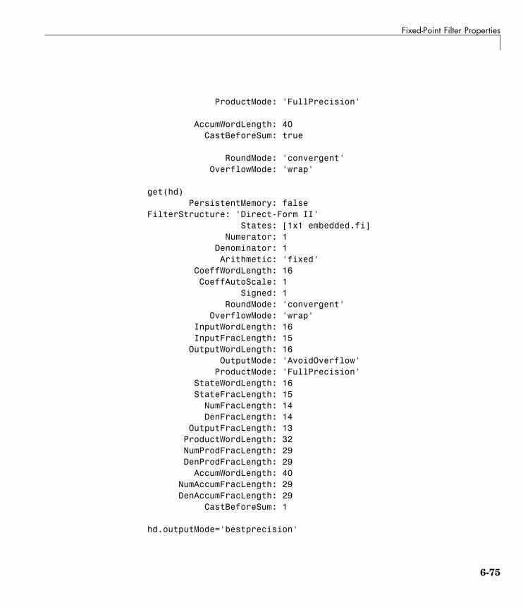
Fixed-Point Filter Properties
ProductMode: 'FullPrecision'
AccumWordLength: 40CastBeforeSum: true
RoundMode: 'convergent'OverflowMode: 'wrap'
get(hd)PersistentMemory: false
FilterStructure: 'Direct-Form II'States: [1x1 embedded.fi]
Numerator: 1Denominator: 1Arithmetic: 'fixed'
CoeffWordLength: 16CoeffAutoScale: 1
Signed: 1RoundMode: 'convergent'
OverflowMode: 'wrap'InputWordLength: 16InputFracLength: 15
OutputWordLength: 16OutputMode: 'AvoidOverflow'
ProductMode: 'FullPrecision'StateWordLength: 16StateFracLength: 15
NumFracLength: 14DenFracLength: 14
OutputFracLength: 13ProductWordLength: 32NumProdFracLength: 29DenProdFracLength: 29
AccumWordLength: 40NumAccumFracLength: 29DenAccumFracLength: 29
CastBeforeSum: 1
hd.outputMode='bestprecision'
6-75

6 Reference for the Properties of Filter Objects
hd =
FilterStructure: 'Direct-Form II'Arithmetic: 'fixed'Numerator: 1
Denominator: 1PersistentMemory: false
States: [1x1 embedded.fi]
CoeffWordLength: 16CoeffAutoScale: true
Signed: true
InputWordLength: 16InputFracLength: 15
OutputWordLength: 16OutputMode: 'BestPrecision'
StateWordLength: 16StateFracLength: 15
ProductMode: 'FullPrecision'
AccumWordLength: 40CastBeforeSum: true
RoundMode: 'convergent'OverflowMode: 'wrap'
hd.outputWordLength=8;
get(hd)PersistentMemory: falseFilterStructure: 'Direct-Form II'
States: [1x1 embedded.fi]Numerator: 1
Denominator: 1Arithmetic: 'fixed'
6-76
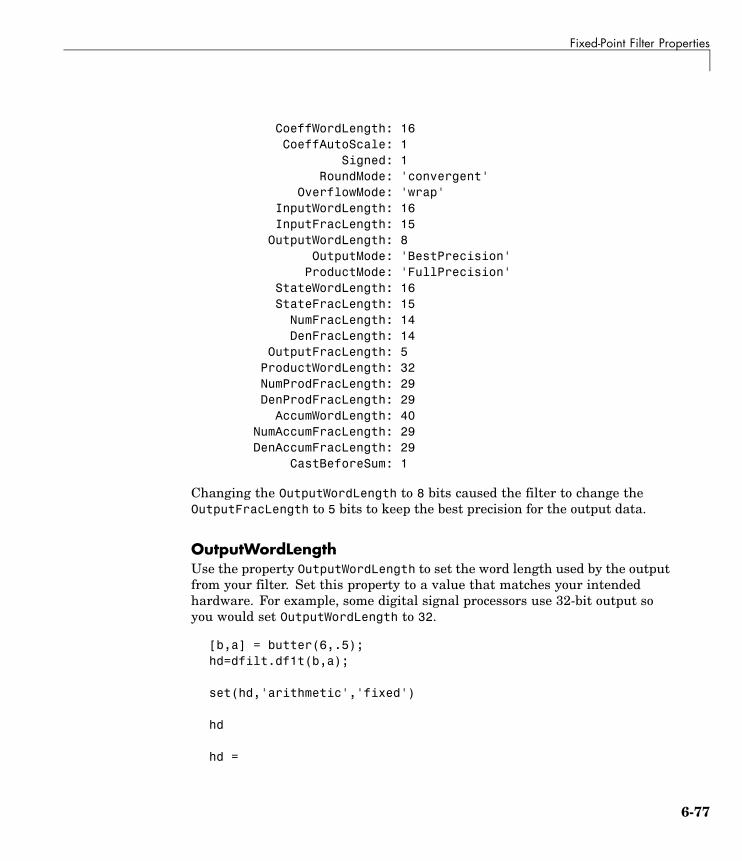
Fixed-Point Filter Properties
CoeffWordLength: 16CoeffAutoScale: 1
Signed: 1RoundMode: 'convergent'
OverflowMode: 'wrap'InputWordLength: 16InputFracLength: 15
OutputWordLength: 8OutputMode: 'BestPrecision'
ProductMode: 'FullPrecision'StateWordLength: 16StateFracLength: 15
NumFracLength: 14DenFracLength: 14
OutputFracLength: 5ProductWordLength: 32NumProdFracLength: 29DenProdFracLength: 29
AccumWordLength: 40NumAccumFracLength: 29DenAccumFracLength: 29
CastBeforeSum: 1
Changing the OutputWordLength to 8 bits caused the filter to change theOutputFracLength to 5 bits to keep the best precision for the output data.
OutputWordLengthUse the property OutputWordLength to set the word length used by the outputfrom your filter. Set this property to a value that matches your intendedhardware. For example, some digital signal processors use 32-bit output soyou would set OutputWordLength to 32.
[b,a] = butter(6,.5);hd=dfilt.df1t(b,a);
set(hd,'arithmetic','fixed')
hd
hd =
6-77

6 Reference for the Properties of Filter Objects
FilterStructure: 'Direct-Form I Transposed'Arithmetic: 'fixed'Numerator: [1x7 double]
Denominator: [1 0 0.7777 0 0.1142 0 0.0018]PersistentMemory: false
States: Numerator: [6x1 fi]Denominator:[6x1 fi]
CoeffWordLength: 16CoeffAutoScale: true
Signed: true
InputWordLength: 16InputFracLength: 15
OutputWordLength: 16OutputMode: 'AvoidOverflow'
MultiplicandWordLength: 16MultiplicandFracLength: 15
StateWordLength: 16StateAutoScale: true
ProductMode: 'FullPrecision'
AccumWordLength: 40CastBeforeSum: true
RoundMode: 'convergent'OverflowMode: 'wrap'
hd.outputwordLength=32
hd =
FilterStructure: 'Direct-Form I Transposed'Arithmetic: 'fixed'
6-78

Fixed-Point Filter Properties
Numerator: [1x7 double]Denominator: [1 0 0.7777 0 0.1142 0 0.0018]
PersistentMemory: falseStates: Numerator: [6x1 fi]
Denominator:[6x1 fi]
CoeffWordLength: 16CoeffAutoScale: true
Signed: true
InputWordLength: 16InputFracLength: 15
OutputWordLength: 32OutputMode: 'AvoidOverflow'
MultiplicandWordLength: 16MultiplicandFracLength: 15
StateWordLength: 16StateAutoScale: true
ProductMode: 'FullPrecision'
AccumWordLength: 40CastBeforeSum: true
RoundMode: 'convergent'OverflowMode: 'wrap'
When you create a filter object, this property starts with the value 16.
OverflowModeThe OverflowMode property is specified as one of the following two stringsindicating how to respond to overflows in fixed-point arithmetic:
• 'saturate' — saturate overflows.
6-79

6 Reference for the Properties of Filter Objects
When the values of data to be quantized lie outside of the range of thelargest and smallest representable numbers (as specified by the applicableword length and fraction length properties), these values are quantized tothe value of either the largest or smallest representable value, dependingon which is closest. saturate is the default value for OverflowMode.
• 'wrap' — wrap all overflows to the range of representable values.
When the values of data to be quantized lie outside of the range of thelargest and smallest representable numbers (as specified by the data formatproperties), these values are wrapped back into that range using modulararithmetic relative to the smallest representable number. You can learnmore about modular arithmetic in Fixed-Point Toolbox documentation.
These rules apply to the OverflowMode property.
• Applies to the accumulator and output data only.
• Does not apply to coefficients or input data. These always saturate theresults.
• Does not apply to products. Products maintain full precision at all times.Your filters do not lose precision in the products.
Note Numbers in floating-point filters that extend beyond the dynamic rangeoverflow to ±inf.
ProductFracLengthAfter you set ProductMode for a fixed-point filter to SpecifyPrecision, thisproperty becomes available for you to change. ProductFracLength sets thefraction length the filter uses for the results of multiplication operations.Only the FIR filters such as asymmetric FIRs or lattice autoregressive filtersinclude this dynamic property.
Your fraction length can be any negative or positive integer, or zero. Inaddition, the fraction length you specify can be larger than the associatedword length. Generally, the default value is 11 bits.
6-80

Fixed-Point Filter Properties
ProductModeThis property, available when your filter is in fixed-point arithmetic mode,specifies how the filter outputs the results of multiplication operations. Alldfilt objects include this property when they use fixed-point arithmetic.
When available, you select from one of the following values for ProductMode:
• FullPrecision — means the filter automatically chooses the word lengthand fraction length it uses to represent the results of multiplicationoperations. The setting allow the product to retain the precision providedby the inputs (multiplicands) to the operation.
• KeepMSB — means you specify the word length for representing productoperation results. The filter sets the fraction length to discard the LSBs,keep the higher order bits in the data, and maintain the precision.
• KeepLSB — means you specify the word length for representing the productoperation results. The filter sets the fraction length to discard the MSBs,keep the lower order bits, and maintain the precision. Compare to theKeepMSB option.
• SpecifyPrecision — means you specify the word length and the fractionlength to apply to data output from product operations.
When you switch to fixed-point filtering from floating-point, you are mostlikely going to throw away some data bits after product operations in yourfilter, perhaps because you have limited resources. When you have to discardsome bits, you might choose to discard the least significant bits (LSB) froma result since the resulting quantization error would be small as the LSBscarry less weight. Or you might choose to keep the LSBs because the resultshave MSBs that are mostly zero, such as when your values are small relativeto the range of the format in which they are represented. So the options forProductMode let you choose how to maintain the information you need fromthe accumulator.
For more information about data formats, word length, and fraction length infixed-point arithmetic, refer to “Notes About Fraction Length, Word Length,and Precision” on page 6-30.
6-81

6 Reference for the Properties of Filter Objects
ProductWordLengthYou use ProductWordLength to define the data word length used by theoutput from multiplication operations. Set this property to a value thatmatches your intended application. For example, the default value is 32 bits,but you can set any word length.
set(hq,'arithmetic','fixed');set(hq,'ProductWordLength',64);
Note that ProductWordLength applies only to filters whose Arithmeticproperty value is fixed.
PersistentMemoryDetermine whether the filter states get restored to their starting values foreach filtering operation. The starting values are the values in place when youcreate the filter object. PersistentMemory returns to zero any state thatthe filter changes during processing. States that the filter does not changeare not affected. Defaults to false — the filter does not retain memoryabout filtering operations from one to the next. Maintaining memory (settingPersistentMemory to true) lets you filter large data sets as collections ofsmaller subsets and get the same result.
In this example, filter hd first filters data xtot in one pass. Then you canuse hd to filter x as two separate data sets. The results ytot and ysec arethe same in both cases.
xtot=[x,x];
ytot=filter(hd,xtot)
ytot =
0 -0.0003 0.0005 -0.0014 0.0028 -0.0054 0.0092
reset(hm1); % Clear history of the filter
hm1.PersistentMemory='true';
ysec=[filter(hd,x) filter(hd,x)]
ysec =
0 -0.0003 0.0005 -0.0014 0.0028 -0.0054 0.0092
6-82

Fixed-Point Filter Properties
This test verifies that ysec (the signal filtered by sections) is equal to ytot(the entire signal filtered at once).
RoundModeThe RoundMode property value specifies the rounding method used forquantizing numerical values. Specify the RoundMode property values as oneof the following five strings.
RoundModeString Description of Rounding Algorithm
'ceil' Round up to the next representable quantized value.
'convergent' Round to the nearest representable quantized value.Numbers that are exactly halfway between the twonearest representable quantized values are rounded upwhen the least significant bit would be set to 1 afterrounding. Otherwise, the number is rounded down. Filterobjects use convergent rounding by default.
'fix' Round negative numbers up and positive numbers downto the next representable quantized value.
'floor' Round down to the next representable quantized value.
'round' Round to the nearest representable quantized value.Numbers that are halfway between the two nearestrepresentable quantized values are rounded up.
The choice you make affects only the accumulator and output arithmetic.Coefficient and input arithmetic always round. Finally, products neveroverflow — they maintain full precision.
ScaleValueFracLengthFilter structures df1sos, df1tsos, df2sos, and df2tsos that use fixedarithmetic have this property that defines the fraction length applied tothe scale values the filter uses between sections. In combination withCoeffWordLength, these two properties fully specify how the filter interpretsand uses the scale values stored in the property ScaleValues. As withfraction length properties, ScaleValueFracLength can be any integer,
6-83
6 Reference for the Properties of Filter Objects
including integers larger than CoeffWordLength, and positive or negativeintegers. 15 bits is the default value when you create the filter.
ScaleValuesThe ScaleValues property values are specified as a scalar (or vector) thatintroduces scaling for inputs (and the outputs from cascaded sections in thevector case) during filtering:
• When you only have a single section in your filter:
- Specify the ScaleValues property value as a scalar if you only want toscale the input to your filter.
- Specify the ScaleValues property as a vector of length 2 if you want tospecify scaling to the input (scaled with the first entry in the vector) andthe output (scaled with the last entry in the vector).
• When you have L cascaded sections in your filter:
- Specify the ScaleValues property value as a scalar if you only want toscale the input to your filter.
- Specify the value for the ScaleValues property as a vector of lengthL+1 if you want to scale the inputs to every section in your filter, alongwith the output:
The first entry of your vector specifies the input scaling
Each successive entry specifies the scaling at the output of the nextsection
The final entry specifies the scaling for the filter output.
The default value for ScaleValues is 0.
The interpretation of this property is described as follows with diagrams in“Interpreting the ScaleValues Property” on page 6-85.
Note The value of the ScaleValues property is not quantized. Data affectedby the presence of a scaling factor in the filter is quantized according to theappropriate data format.
6-84

Fixed-Point Filter Properties
When you apply normalize to a fixed-point filter, the value for theScaleValues property is changed accordingly.
It is good practice to choose values for this property that are either positive ornegative powers of two.
Interpreting the ScaleValues Property. When you specify the values ofthe ScaleValues property of a quantized filter, the values are entered as avector, the length of which is determined by the number of cascaded sectionsin your filter:
• When you have only one section, the value of the Scalevalues property canbe a scalar or a two-element vector.
• When you have L cascaded sections in your filter, the value of theScaleValues property can be a scalar or an L+1-element vector.
The following diagram shows how the ScaleValues property values areapplied to a quantized filter with only one section.
The following diagram shows how the ScaleValues property values areapplied to a quantized filter with two sections.
6-85

6 Reference for the Properties of Filter Objects
SignedWhen you create a dfilt object for fixed-point filtering (you set the propertyArithmetic to fixed, the property Signed specifies whether the filterinterprets coefficients as signed or unsigned. This setting applies only to thecoefficients. While the default setting is true, meaning that all coefficientsare assumed to be signed, you can change the setting to false after youcreate the fixed-point filter.
For example, create a fixed-point direct-form II transposed filter with bothnegative and positive coefficients, and then change the property value forSigned from true to false to see what happens to the negative coefficientvalues.
hd=dfilt.df2t(-5:5)
hd =
FilterStructure: 'Direct-Form II Transposed'Arithmetic: 'double'Numerator: [-5 -4 -3 -2 -1 0 1 2 3 4 5]
Denominator: 1PersistentMemory: false
States: [10x1 double]
set(hd,'arithmetic','fixed')hd.numerator
ans =
-5 -4 -3 -2 -1 0
6-86

Fixed-Point Filter Properties
1 2 3 4 5
set(hd,'signed',false)hd.numerator
ans =
0 0 0 0 0 01 2 3 4 5
Using unsigned coefficients limits you to using only positive coefficients inyour filter. Signed is a dynamic property — you cannot set or change it untilyou switch the setting for the Arithmetic property to fixed.
SosMatrixWhen you convert a dfilt object to second-order section form, or create asecond-order section filter, sosMatrix holds the filter coefficients as propertyvalues. Using the double data type by default, the matrix is in [sectionscoefficients per section] form, displayed as [15-x-6] for filters with 6coefficients per section and 15 sections, [15 6].
To demonstrate, the following code creates an order 30 filter usingsecond-order sections in the direct-form II transposed configuration. Noticethe sosMatrix property contains the coefficients for all the sections.
d = fdesign.lowpass('n,fc',30,0.5);hd = butter(d);
hd =
FilterStructure: 'Direct-Form II, Second-Order Sections'Arithmetic: 'double'sosMatrix: [15x6 double]
ScaleValues: [16x1 double]PersistentMemory: false
States: [2x15 double]
hd.arithmetic='fixed'
hd =
6-87

6 Reference for the Properties of Filter Objects
FilterStructure: 'Direct-Form II, Second-Order Sections'Arithmetic: 'fixed'sosMatrix: [15x6 double]
ScaleValues: [16x1 double]PersistentMemory: false
States: [1x1 embedded.fi]
CoeffWordLength: 16CoeffAutoScale: true
Signed: true
InputWordLength: 16InputFracLength: 15
SectionInputWordLength: 16SectionInputAutoScale: true
SectionOutputWordLength: 16SectionOutputAutoScale: true
OutputWordLength: 16OutputMode: 'AvoidOverflow'
StateWordLength: 16StateFracLength: 15
ProductMode: 'FullPrecision'
AccumWordLength: 40CastBeforeSum: true
RoundMode: 'convergent'OverflowMode: 'wrap'
hd.sosMatrix
ans =
1.0000 2.0000 1.0000 1.0000 0 0.9005
6-88

Fixed-Point Filter Properties
1.0000 2.0000 1.0000 1.0000 0 0.72941.0000 2.0000 1.0000 1.0000 0 0.58881.0000 2.0000 1.0000 1.0000 0 0.47241.0000 2.0000 1.0000 1.0000 0 0.37551.0000 2.0000 1.0000 1.0000 0 0.29481.0000 2.0000 1.0000 1.0000 0 0.22751.0000 2.0000 1.0000 1.0000 0 0.17161.0000 2.0000 1.0000 1.0000 0 0.12541.0000 2.0000 1.0000 1.0000 0 0.08781.0000 2.0000 1.0000 1.0000 0 0.05761.0000 2.0000 1.0000 1.0000 0 0.03441.0000 2.0000 1.0000 1.0000 0 0.01731.0000 2.0000 1.0000 1.0000 0 0.00621.0000 2.0000 1.0000 1.0000 0 0.0007
The SOS matrix is an M-by-6 matrix, where M is the number of sections inthe second-order section filter. Filter hd has M equal to 15 as shown above (15rows). Each row of the SOS matrix contains the numerator and denominatorcoefficients (b’s and a’s) and the scale factors of the corresponding sectionin the filter.
SectionInputAutoScaleSecond-order section filters include this property that determines who thefilter handles data in the transitions from one section to the next in the filter.
How the filter represents the data passing from one section to thenext depends on the property value of SectionInputAutoScale. Therepresentation the filter uses between the filter sections depends on whetherthe value of SectionInputAutoScale is true or false.
• SectionInputAutoScale = true means the filter chooses the fractionlength to maintain the value of the data between sections as close to theoutput values from the previous section as possible. true is the defaultsetting.
• SectionInputAutoScale = false removes the automatic scaling of thefraction length for the intersection data and exposes the property thatcontrols the coefficient fraction length (SectionInputFracLength) soyou can change it. For example, if the filter is a second-order, directform FIR filter, setting SectionInputAutoScale to false exposes the
6-89

6 Reference for the Properties of Filter Objects
SectionInputFracLength property that specifies the fraction lengthapplied to data between the sections.
SectionInputFracLengthSecond-order section filters use quantizers at the input to each sectionof the filter. The quantizers apply to the input data entering each filtersection. Note that the quantizers for each section are the same. To set thefraction length for interpreting the input values, use the property value inSectionInputFracLength.
In combination with CoeffWordLength, SectionInputFracLength fullydetermines how the filter interprets and uses the state values stored inthe property States. As with all word and fraction length properties,SectionInputFracLength can be any integer, including integers larger thanCoeffWordLength, and positive or negative integers. 15 bits is the defaultvalue when you create the filter object.
SectionInputWordLengthSOS filters are composed of sections, each one a second-order filter. Filteringdata input to the filter involves passing the data through each filter section.SectionInputWordLength specifies the word length applied to data asit enters one filter section from the previous section. Only second-orderimplementations of direct-form I transposed and direct-form II transposedfilters include this property.
The following diagram shows an SOS filter composed of sections (the bottompart of the diagram) and a possible internal structure of each Section (the topportion of the diagram), in this case — a direct form I transposed second ordersections filter structure. Note that the output of each section is fed througha multiplier. If the gain of the multiplier =1, then the last Cast block of theSection is ignored, and the format of the output is NumSumQ.
6-90

Fixed-Point Filter Properties
�������
������
��� �� ����
�������
�������
���������� �����
��������� ���������������� ������
�������
��������
������
�������
��� ���
�������
�������
������
��������
�������
�������
�������� ��������
��������������
���� ����
����� ���������� �� ���� ��!�" �"
���� ������ ���� ����� ���� ���� ���� �����
�"���
6-91

6 Reference for the Properties of Filter Objects
SectionInputWordLength defaults to 16 bits.
SectionOutputAutoScaleSecond-order section filters include this property that determines who thefilter handles data in the transitions from one section to the next in the filter.
How the filter represents the data passing from one section to thenext depends on the property value of SectionOutputAutoScale. Therepresentation the filter uses between the filter sections depends on whetherthe value of SectionOutputAutoScale is true or false.
• SectionOutputAutoScale = true means the filter chooses the fractionlength to maintain the value of the data between sections as close to theoutput values from the previous section as possible. true is the defaultsetting.
• SectionOutputAutoScale = false removes the automatic scaling of thefraction length for the intersection data and exposes the property thatcontrols the coefficient fraction length (SectionOutputFracLength) soyou can change it. For example, if the filter is a second-order, directform FIR filter, setting SectionOutputAutoScale = false exposes theSectionOutputFracLength property that specifies the fraction lengthapplied to data between the sections.
SectionOutputFracLengthSecond-order section filters use quantizers at the output from each sectionof the filter. The quantizers apply to the output data leaving each filtersection. Note that the quantizers for each section are the same. To set thefraction length for interpreting the output values, use the property value inSectionOutputFracLength.
In combination with CoeffWordLength, SectionOutputFracLengthdetermines how the filter interprets and uses the state values storedin the property States. As with all fraction length properties,SectionOutputFracLength can be any integer, including integers larger thanCoeffWordLength, and positive or negative integers. 15 bits is the defaultvalue when you create the filter object.
6-92

Fixed-Point Filter Properties
SectionOutputWordLengthSOS filters are composed of sections, each one a second-order filter. Filteringdata input to the filter involves passing the data through each filter section.SectionOutputWordLength specifies the word length applied to data as itleaves one filter section to go to the next. Only second-order implementationsdirect-form I transposed and direct-form II transposed filters include thisproperty.
The following diagram shows an SOS filter composed of sections (the bottompart of the diagram) and a possible internal structure of each Section (the topportion of the diagram), in this case — a direct form I transposed second ordersections filter structure. Note that the output of each section is fed througha multiplier. If the gain of the multiplier =1, then the last Cast block of theSection is ignored, and the format of the output is NumSumQ.
6-93

6 Reference for the Properties of Filter Objects
�������
������
��� �� ����
�������
�������
���������� �����
��������� ���������������� ������
�������
��������
������
�������
��� ���
�������
�������
������
��������
�������
�������
�������� ��������
��������������
���� ����
����� ���������� �� ���� ��!�" �"
���� ������ ���� ����� ���� ���� ���� �����
�"���
6-94

Fixed-Point Filter Properties
SectionOutputWordLength defaults to 16 bits.
StateAutoScaleAlthough all filters use states, some do not allow you to choose whetherthe filter automatically scales the state values to prevent overruns or badarithmetic errors. You select either of the following settings:
• StateAutoScale = true means the filter chooses the fraction length tomaintain the value of the states as close to the double-precision values aspossible. When you change the word length applied to the states (whereallowed by the filter structure), the filter object changes the fraction lengthto try to accommodate the change. true is the default setting.
• StateAutoScale = false removes the automatic scaling of the fractionlength for the states and exposes the property that controls the coefficientfraction length so you can change it. For example, in a direct form Itransposed SOS FIR filter, setting StateAutoScale = false exposes theNumStateFracLength and DenStateFracLength properties that specifythe fraction length applied to states.
Each of the following filter structures provides the StateAutoScale property:
• df1t
• df1tsos
• df2t
• df2tsos
• dffirt
Other filter structures do not include this property.
StateFracLengthFilter states stored in the property States have both word length and fractionlength. To set the fraction length for interpreting the stored filter object statevalues, use the property value in StateFracLength.
6-95

6 Reference for the Properties of Filter Objects
In combination with CoeffWordLength, StateFracLength fully determineshow the filter interprets and uses the state values stored in the propertyStates.
As with all fraction length properties, StateFracLength can be any integer,including integers larger than CoeffWordLength, and positive or negativeintegers. 15 bits is the default value when you create the filter object.
StatesDigital filters are dynamic systems. The behavior of dynamic systems (theirresponse) depends on the input (stimulus) to the system and the current orprevious state of the system. You can say the system has memory or inertia.All fixed- or floating-point digital filters (as well as analog filters) have states.
Filters use the states to compute the filter output for each input sample, aswell using them while filtering in loops to maintain the filter state betweenloop iterations. This toolbox assumes zero-valued initial conditions (thedynamic system is at rest) by default when you filter the first input sample.Assuming the states are zero initially does not mean the states are not used;they are, but arithmetically they do not have any effect.
Filter objects store the state values in the property States. The number ofstored states depends on the filter implementation, since the states representthe delays in the filter implementation.
When you review the display for a filter object with fixed arithmetic, noticethat the states return an embedded fi object, as you see here.
b = ellip(6,3,50,300/500);
hd=dfilt.dffir(b)
hd =
FilterStructure: 'Direct-Form FIR'
Arithmetic: 'double'
Numerator: [0.0773 0.2938 0.5858 0.7239 0.5858 0.2938 0.0773]
PersistentMemory: false
States: [6x1 double]
6-96

Fixed-Point Filter Properties
hd.arithmetic='fixed'
hd =
FilterStructure: 'Direct-Form FIR'
Arithmetic: 'fixed'
Numerator: [0.0773 0.2938 0.5858 0.7239 0.5858 0.2938 0.0773]
PersistentMemory: false
States: [1x1 embedded.fi]
CoeffWordLength: 16
CoeffAutoScale: 'on'
Signed: 'on'
InputWordLength: 16
InputFracLength: 15
OutputWordLength: 16
OutputMode: 'AvoidOverflow'
ProductMode: 'FullPrecision'
AccumWordLength: 40
CastBeforeSum: 'on'
RoundMode: 'convergent'
OverflowMode: 'wrap'
InheritSettings: 'off'
fi objects provide fixed-point support for the filters. To learn more about thedetails about fi objects, refer to your Fixed-Point Toolbox documentation.
The property States lets you use a fi object to define how the filter interpretsthe filter states. For example, you can create a fi object in MATLAB, thenassign the object to States, as follows:
statefi=fi([],16,12)
6-97

6 Reference for the Properties of Filter Objects
statefi =
[]DataTypeMode = Fixed-point: binary point scaling
Signed = trueWordlength = 16
Fractionlength = 12
This fi object does not have a value associated (notice the [] input argumentto fi for the value), and it has word length of 16 bits and fraction length of 12bit. Now you can apply statefi to the States property of the filter hd.
set(hd,'States',statefi);Warning: The 'States' property will be reset to the valuespecified at construction before filtering.Set the 'PersistentMemory' flag to 'True'to avoid changing this property value.hd
hd =
FilterStructure: 'Direct-Form FIR'Arithmetic: 'fixed'Numerator: [0.0773 0.2938 0.5858 0.7239 0.5858
0.2938 0.0773]PersistentMemory: false
States: [1x1 embedded.fi]
CoeffWordLength: 16CoeffAutoScale: 'on'
Signed: 'on'
InputWordLength: 16InputFracLength: 15
OutputWordLength: 16OutputMode: 'AvoidOverflow'
ProductMode: 'FullPrecision'AccumWordLength: 40
6-98

Fixed-Point Filter Properties
CastBeforeSum: 'on'
RoundMode: 'convergent'OverflowMode: 'wrap'
StateWordLengthWhile all filters use states, some do not allow you to directly change the staterepresentation — the word length and fraction lengths — independently. Forthe others, StateWordLength specifies the word length, in bits, the filter usesto represent the states. Filters that do not provide direct state word lengthcontrol include:
• df1
• dfasymfir
• dffir
• dfsymfir
For these structures, the filter derives the state format from the input formatyou choose for the filter — except for the df1 IIR filter. In this case, thenumerator state format comes from the input format and the denominatorstate format comes from the output format. All other filter structures providecontrol of the state format directly.
TapSumFracLengthDirect-form FIR filter objects, both symmetric and antisymmetric, use thisproperty. To set the fraction length for output from the sum operations thatinvolve the filter tap weights, use the property value in TapSumFracLength. Toenable this property, set the TapSumMode to SpecifyPrecision in your filter.
As you can see in this code example that creates a fixed-point asymmetric FIRfilter, the TapSumFracLength property becomes available after you change theTapSumMode property value.
hd=dfilt.dfasymfir
hd =
6-99

6 Reference for the Properties of Filter Objects
FilterStructure: 'Direct-Form Antisymmetric FIR'Arithmetic: 'double'Numerator: 1
PersistentMemory: falseStates: [0x1 double]
set(hd,'arithmetic','fixed');hd
hd =
FilterStructure: 'Direct-Form Antisymmetric FIR'Arithmetic: 'fixed'Numerator: 1
PersistentMemory: falseStates: [1x1 embedded.fi]
CoeffWordLength: 16CoeffAutoScale: true
Signed: true
InputWordLength: 16InputFracLength: 15
OutputWordLength: 16OutputMode: 'AvoidOverflow'
TapSumMode: 'KeepMSB'TapSumWordLength: 17
ProductMode: 'FullPrecision'
AccumWordLength: 40
CastBeforeSum: trueRoundMode: 'convergent'
OverflowMode: 'wrap'
6-100
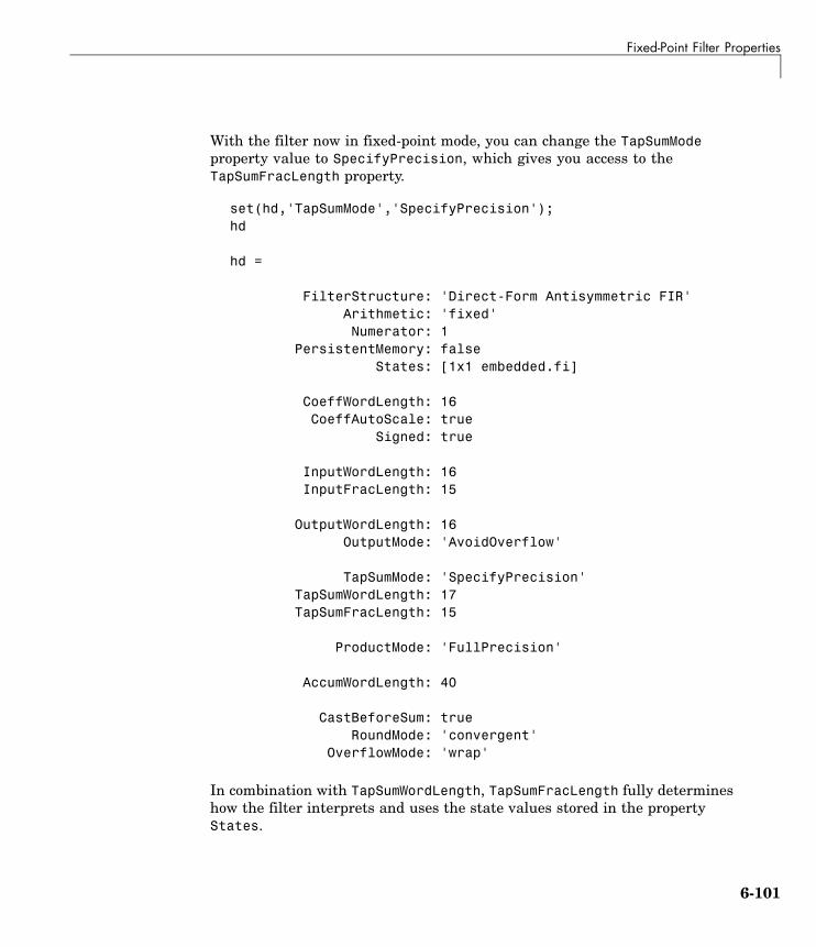
Fixed-Point Filter Properties
With the filter now in fixed-point mode, you can change the TapSumModeproperty value to SpecifyPrecision, which gives you access to theTapSumFracLength property.
set(hd,'TapSumMode','SpecifyPrecision');hd
hd =
FilterStructure: 'Direct-Form Antisymmetric FIR'Arithmetic: 'fixed'Numerator: 1
PersistentMemory: falseStates: [1x1 embedded.fi]
CoeffWordLength: 16CoeffAutoScale: true
Signed: true
InputWordLength: 16InputFracLength: 15
OutputWordLength: 16OutputMode: 'AvoidOverflow'
TapSumMode: 'SpecifyPrecision'TapSumWordLength: 17TapSumFracLength: 15
ProductMode: 'FullPrecision'
AccumWordLength: 40
CastBeforeSum: trueRoundMode: 'convergent'
OverflowMode: 'wrap'
In combination with TapSumWordLength, TapSumFracLength fully determineshow the filter interprets and uses the state values stored in the propertyStates.
6-101
6 Reference for the Properties of Filter Objects
As with all fraction length properties, TapSumFracLength can be any integer,including integers larger than TapSumWordLength, and positive or negativeintegers. 15 bits is the default value when you create the filter object.
TapSumModeThis property, available only after your filter is in fixed-point mode, specifieshow the filter outputs the results of summation operations that involve thefilter tap weights. Only symmetric (dfilt.dfsymfir) and antisymmetric(dfilt.dfasymfir) FIR filters use this property.
When available, you select from one of the following values:
• FullPrecision — means the filter automatically chooses the word lengthand fraction length to represent the results of the sum operation so theyretain all of the precision provided by the inputs (addends).
• KeepMSB — means you specify the word length for representing tap sumsummation results to keep the higher order bits in the data. The filter setsthe fraction length to discard the LSBs from the sum operation. This isthe default property value.
• KeepLSB — means you specify the word length for representing tap sumsummation results to keep the lower order bits in the data. The filter setsthe fraction length to discard the MSBs from the sum operation. Compareto the KeepMSB option.
• SpecifyPrecision — means you specify the word and fraction lengths toapply to data output from the tap sum operations.
TapSumWordLengthSpecifies the word length the filter uses to represent the output from tapsum operations. The default value is 17 bits. Only dfasymfir and dfsymfirfilters include this property.
6-102

Adaptive Filter Properties
Adaptive Filter Properties
In this section...
“Property Summaries” on page 6-103
“Property Details for Adaptive Filter Properties” on page 6-108
Property SummariesThe following table summarizes the adaptive filter properties and provides abrief description of each. Full descriptions of each property, in alphabeticalorder, are given in the subsequent section.
Property Description
Algorithm Reports the algorithm the object uses foradaptation. When you construct your adaptivefilter object, this property is set automaticallyby the constructor, such as adaptfilt.nlmscreating an adaptive filter that uses thenormalized LMS algorithm. You cannot changethe value — it is read only.
AvgFactor Averaging factor used to compute theexponentially-windowed estimates of the powersin the transformed signal bins for the coefficientupdates. AvgFactor should lie between zero andone. For default filter objects, AvgFactor equals(1 - step). lambda is the input argument thatrepresents AvgFactor
BkwdPredErrorPower Returns the minimum mean-squared predictionerror. Refer to [2] in the bibliography for detailsabout linear prediction.
BkwdPrediction Returns the predicted samples generated duringadaptation. Refer to [2] in the bibliography fordetails about linear prediction.
6-103

6 Reference for the Properties of Filter Objects
Property Description
Blocklength Block length for the coefficient updates.This must be a positive integer such that(l/blocklength) is also an integer. For fasterexecution, blocklength should be a power oftwo. blocklength defaults to two.
Coefficients Vector containing the initial filter coefficients. Itmust be a length l vector where l is the numberof filter coefficients. coeffs defaults to lengthl vector of zeros when you do not provide theargument for input.
ConversionFactor Conversion factor defaults to the matrix [1 -1]that specifies soft-constrained initialization.This is the gamma input argument for some ofthe fast transversal algorithms.
Delay Update delay given in time samples. Thisscalar should be a positive integer—negativedelays do not work. delay defaults to 1 for mostalgorithms.
DesiredSignalStates Desired signal states of the adaptive filter.dstates defaults to a zero vector with lengthequal to (blocklen - 1) or (swblocklen - 1)depending on the algorithm.
EpsilonStates Vector of the epsilon values of the adaptive filter.EpsilonStates defaults to a vector of zeros with(projectord - 1) elements.
ErrorStates Vector of the adaptive filter error states.ErrorStates defaults to a zero vector withlength equal to (projectord - 1).
FFTCoefficients Stores the discrete Fourier transform of thefilter coefficients in coeffs.
FFTStates Stores the states of the FFT of the filtercoefficients during adaptation.
FilteredInputStates Vector of filtered input states with length equalto l - 1.
6-104

Adaptive Filter Properties
Property Description
FilterLength Contains the length of the filter. Note that thisis not the filter order. Filter length is 1 greaterthan filter order. Thus a filter with length equalto 10 has filter order equal to 9.
ForgettingFactor Determines how the RLS adaptive filter usespast data in each iteration. You use theforgetting factor to specify whether old datacarries the same weight in the algorithm asmore recent data.
FwdPredErrorPower Returns the minimum mean-squared predictionerror in the forward direction. Refer to [2] in thebibliography for details about linear prediction.
FwdPrediction Contains the predicted values for samplesduring adaptation. Compare these to the actualsamples to get the error and power.
InitFactor Soft-constrained initialization factor. This scalarshould be positive and sufficiently large toprevent an excessive number of Kalman gainrescues. Called delta as an input argument,this defaults to one.
InvCov Upper-triangular Cholesky (square root) factorof the input covariance matrix. Initialize thismatrix with a positive definite upper triangularmatrix. Dimensions are l-by-l, where l is thefilter length.
KalmanGain Empty when you construct the object, this getspopulated after you run the filter.
KalmanGainStates Contains the states of the Kalman gain updatesduring adaptation.
6-105

6 Reference for the Properties of Filter Objects
Property Description
Leakage Contains the setting for leakage in the adaptivefilter algorithm. Using a leakage factor that isnot 1 forces the weights to adapt even when theyhave found the minimum error solution. Forcingthe adaptation can improve the numericalperformance of the LMS algorithm.
OffsetCov Contains the offset covariance matrix.
Offset Specifies an optional offset for the denominatorof the step size normalization term. You mustspecify offset to be a scalar greater than orequal to zero. Nonzero offsets can help avoid adivide-by-near-zero condition that causes errors.
Power A vector of 2*l elements, each initialized withthe value delta from the input arguments. Asyou filter data, Power gets updated by the filterprocess.
ProjectionOrder Projection order of the affine projectionalgorithm. projectord defines the size of theinput signal covariance matrix and defaults totwo.
ReflectionCoeffs Coefficients determined for the reflection portionof the filter during adaptation.
ReflectionCoeffsStep Size of the steps used to determine the reflectioncoefficients.
PersistentMemory Specifies whether to reset the filter states andmemory before each filtering operation. Letsyou decide whether your filter retains states andcoefficients from previous filtering runs.
SecondaryPathCoeffs A vector that contains the coefficient values ofyour secondary path from the output actuatorto the error sensor.
SecondaryPathEstimate An estimate of the secondary path filter model.
6-106
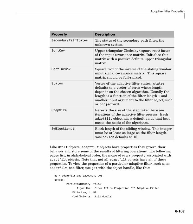
Adaptive Filter Properties
Property Description
SecondaryPathStates The states of the secondary path filter, theunknown system.
SqrtCov Upper-triangular Cholesky (square root) factorof the input covariance matrix. Initialize thismatrix with a positive definite upper triangularmatrix.
SqrtlnvCov Square root of the inverse of the sliding windowinput signal covariance matrix. This squarematrix should be full-ranked.
States Vector of the adaptive filter states. statesdefaults to a vector of zeros whose lengthdepends on the chosen algorithm. Usually thelength is a function of the filter length l andanother input argument to the filter object, suchas projectord.
StepSize Reports the size of the step taken betweeniterations of the adaptive filter process. Eachadaptfilt object has a default value that bestmeets the needs of the algorithm.
SwBlockLength Block length of the sliding window. This integermust be at least as large as the filter length.swblocklen defaults to 16.
Like dfilt objects, adaptfilt objects have properties that govern theirbehavior and store some of the results of filtering operations. The followingpages list, in alphabetical order, the name of every property associated withadaptfilt objects. Note that not all adaptfilt objects have all of theseproperties. To view the properties of a particular adaptive filter, such as anadaptfilt.bap filter, use get with the object handle, like this:
ha = adaptfilt.bap(32,0.5,4,1.0);
get(ha)
PersistentMemory: false
Algorithm: 'Block Affine Projection FIR Adaptive Filter'
FilterLength: 32
Coefficients: [1x32 double]
6-107

6 Reference for the Properties of Filter Objects
States: [35x1 double]
StepSize: 0.5000
ProjectionOrder: 4
OffsetCov: [4x4 double]
get shows you the properties for ha and the values for the properties.Entering the object handle returns the same values and properties withoutthe formatting of the list and the more familiar property names.
Property Details for Adaptive Filter Properties
AlgorithmReports the algorithm the object uses for adaptation. When you construct youadaptive filter object, this property is set automatically. You cannot changethe value—it is read only.
AvgFactorAveraging factor used to compute the exponentially-windowed estimates of thepowers in the transformed signal bins for the coefficient updates. AvgFactorshould lie between zero and one. For default filter objects, AvgFactor equals(1 - step). lambda is the input argument that represent AvgFactor
BkwdPredErrorPowerReturns the minimum mean-squared prediction error in the backwarddirection. Refer to [2] in the bibliography for details about linear prediction.
BkwdPredictionWhen you use an adaptive filter that does backward prediction, such asadaptfilt.ftf, one property of the filter contains the backward predictioncoefficients for the adapted filter. With these coefficient, the forwardcoefficients, and the system under test, you have the full set of knowledge ofhow the adaptation occurred. Two values stored in properties compose theBkwdPrediction property:
• Coefficients, which contains the coefficients of the system under test, asdetermined using backward predictions process.
6-108

Adaptive Filter Properties
• Error, which is the difference between the filter coefficients determined bybackward prediction and the actual coefficients of the sample filter. Inthis example, adaptfilt.ftf identifies the coefficients of an unknownFIR system.
x = randn(1,500); % Input to the filter
b = fir1(31,0.5); % FIR system to be identified
n = 0.1*randn(1,500); % Observation noise signal
d = filter(b,1,x)+n; % Desired signal
N = 31; % Adaptive filter order
lam = 0.99; % RLS forgetting factor
del = 0.1; % Soft-constrained initialization factor
ha = adaptfilt.ftf(32,lam,del);
[y,e] = filter(ha,x,d);
ha
ha =
Algorithm: 'Fast Transversal Least-Squares Adaptive Filter'
FilterLength: 32
Coefficients: [1x32 double]
States: [31x1 double]
ForgettingFactor: 0.9900
InitFactor: 0.1000
FwdPrediction: [1x1 struct]
BkwdPrediction: [1x1 struct]
KalmanGain: [32x1 double]
ConversionFactor: 0.7338
KalmanGainStates: [32x1 double]
PersistentMemory: false
ha.coefficients
ans =
Columns 1 through 8
-0.0055 0.0048 0.0045 0.0146 -0.0009 0.0002 -0.0019 0.0008
6-109

6 Reference for the Properties of Filter Objects
Columns 9 through 16
-0.0142 -0.0226 0.0234 0.0421 -0.0571 -0.0807 0.1434 0.4620
Columns 17 through 24
0.4564 0.1532 -0.0879 -0.0501 0.0331 0.0361 -0.0266 -0.0220
Columns 25 through 32
0.0231 0.0026 -0.0063 -0.0079 0.0032 0.0082 0.0033 0.0065
ha.bkwdprediction
ans =
Coeffs: [1x32 double]
Error: 82.3394
>> ha.bkwdprediction.coeffs
ans =
Columns 1 through 8
0.0067 0.0186 0.1114 -0.0150 -0.0239 -0.0610 -0.1120 -0.1026
Columns 9 through 16
0.0093 -0.0399 -0.0045 0.0622 0.0997 0.0778 0.0646 -0.0564
Columns 17 through 24
0.0775 0.0814 0.0057 0.0078 0.1271 -0.0576 0.0037 -0.0200
Columns 25 through 32
-0.0246 0.0180 -0.0033 0.1222 0.0302 -0.0197 -0.1162 0.0285
6-110
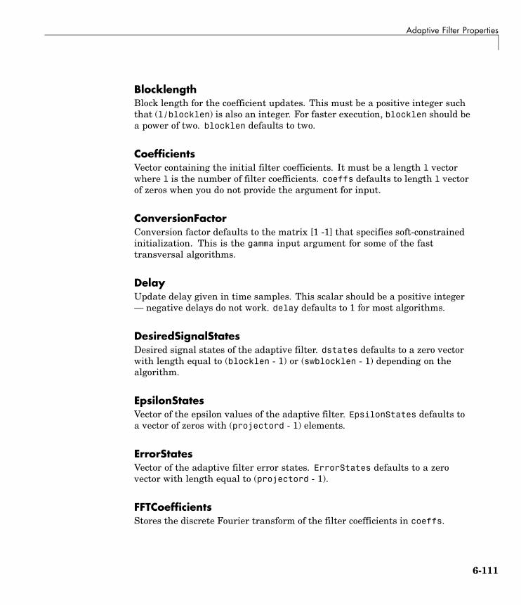
Adaptive Filter Properties
BlocklengthBlock length for the coefficient updates. This must be a positive integer suchthat (l/blocklen) is also an integer. For faster execution, blocklen should bea power of two. blocklen defaults to two.
CoefficientsVector containing the initial filter coefficients. It must be a length l vectorwhere l is the number of filter coefficients. coeffs defaults to length l vectorof zeros when you do not provide the argument for input.
ConversionFactorConversion factor defaults to the matrix [1 -1] that specifies soft-constrainedinitialization. This is the gamma input argument for some of the fasttransversal algorithms.
DelayUpdate delay given in time samples. This scalar should be a positive integer— negative delays do not work. delay defaults to 1 for most algorithms.
DesiredSignalStatesDesired signal states of the adaptive filter. dstates defaults to a zero vectorwith length equal to (blocklen - 1) or (swblocklen - 1) depending on thealgorithm.
EpsilonStatesVector of the epsilon values of the adaptive filter. EpsilonStates defaults toa vector of zeros with (projectord - 1) elements.
ErrorStatesVector of the adaptive filter error states. ErrorStates defaults to a zerovector with length equal to (projectord - 1).
FFTCoefficientsStores the discrete Fourier transform of the filter coefficients in coeffs.
6-111
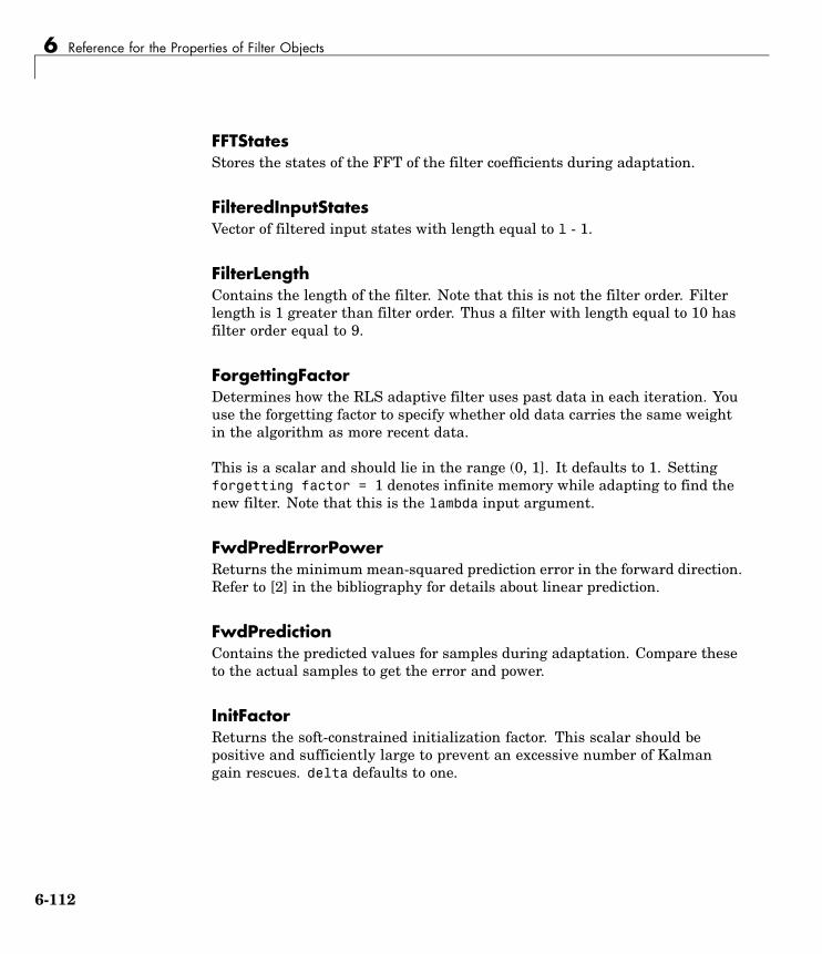
6 Reference for the Properties of Filter Objects
FFTStatesStores the states of the FFT of the filter coefficients during adaptation.
FilteredInputStatesVector of filtered input states with length equal to l - 1.
FilterLengthContains the length of the filter. Note that this is not the filter order. Filterlength is 1 greater than filter order. Thus a filter with length equal to 10 hasfilter order equal to 9.
ForgettingFactorDetermines how the RLS adaptive filter uses past data in each iteration. Youuse the forgetting factor to specify whether old data carries the same weightin the algorithm as more recent data.
This is a scalar and should lie in the range (0, 1]. It defaults to 1. Settingforgetting factor = 1 denotes infinite memory while adapting to find thenew filter. Note that this is the lambda input argument.
FwdPredErrorPowerReturns the minimum mean-squared prediction error in the forward direction.Refer to [2] in the bibliography for details about linear prediction.
FwdPredictionContains the predicted values for samples during adaptation. Compare theseto the actual samples to get the error and power.
InitFactorReturns the soft-constrained initialization factor. This scalar should bepositive and sufficiently large to prevent an excessive number of Kalmangain rescues. delta defaults to one.
6-112

Adaptive Filter Properties
InvCovUpper-triangular Cholesky (square root) factor of the input covariancematrix. Initialize this matrix with a positive definite upper triangular matrix.Dimensions are l-by-l, where l is the filter length.
KalmanGainEmpty when you construct the object, this gets populated after you run thefilter.
KalmanGainStatesContains the states of the Kalman gain updates during adaptation.
LeakageContains the setting for leakage in the adaptive filter algorithm. Using aleakage factor that is not 1 forces the weights to adapt even when they havefound the minimum error solution. Forcing the adaptation can improve thenumerical performance of the LMS algorithm.
OffsetCovContains the offset covariance matrix.
OffsetSpecifies an optional offset for the denominator of the step size normalizationterm. You must specify offset to be a scalar greater than or equal to zero.Nonzero offsets can help avoid a divide-by-near-zero condition that causeserrors.
Use this to avoid dividing by zero or by very small numbers when input signalamplitude becomes very small, or dividing by very small numbers when anyof the FFT input signal powers become very small. offset defaults to one.
PowerA vector of 2*l elements, each initialized with the value delta from the inputarguments. As you filter data, Power gets updated by the filter process.
6-113

6 Reference for the Properties of Filter Objects
ProjectionOrderProjection order of the affine projection algorithm. projectord defines thesize of the input signal covariance matrix and defaults to two.
ReflectionCoeffsFor adaptive filters that use reflection coefficients, this property stores them.
ReflectionCoeffsStepAs the adaptive filter changes coefficient values during adaptation, the stepsize used between runs is stored here.
PersistentMemoryDetermines whether the filter states and coefficients get restored to theirstarting values for each filtering operation. The starting values are the valuesin place when you create the filter.
PersistentMemory returns to zero any property value that the filter changesduring processing. Property values that the filter does not change are notaffected. Defaults to false.
SecondaryPathCoeffsA vector that contains the coefficient values of your secondary path from theoutput actuator to the error sensor.
SecondaryPathEstimateAn estimate of the secondary path filter model.
SecondaryPathStatesThe states of the secondary path filter, the unknown system.
SqrtCovUpper-triangular Cholesky (square root) factor of the input covariance matrix.Initialize this matrix with a positive definite upper triangular matrix.
6-114

Adaptive Filter Properties
SqrtInvCovSquare root of the inverse of the sliding window input signal covariancematrix. This square matrix should be full-ranked.
StatesVector of the adaptive filter states. states defaults to a vector of zeros whoselength depends on the chosen algorithm. Usually the length is a functionof the filter length l and another input argument to the filter object, suchas projectord.
StepSizeReports the size of the step taken between iterations of the adaptive filterprocess. Each adaptfilt object has a default value that best meets the needsof the algorithm.
SwBlockLengthBlock length of the sliding window. This integer must be at least as large asthe filter length. swblocklength defaults to 16.
6-115

6 Reference for the Properties of Filter Objects
Multirate Filter Properties
In this section...
“Property Summaries” on page 6-116
“Property Details for Multirate Filter Properties” on page 6-121
Property SummariesThe following table summarizes the multirate filter properties and providesa brief description of each. Full descriptions of each property are given inthe subsequent section.
Name Values Default Description
BlockLength Positive integers 100 Length of each block of datainput to the FFT used inthe filtering. fftfirinterpmultirate filters includethis property.
DecimationFactor Any positive integer 2 Amount to reduce the inputsampling rate.
DifferentialDelay Any integer 1 Sets the differential delayfor the filter. Usuallya value of one or two isappropriate.
6-116
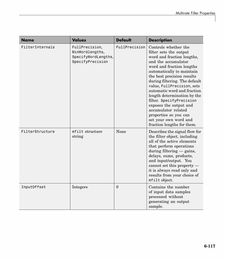
Multirate Filter Properties
Name Values Default Description
FilterInternals FullPrecision,MinWordlengths,SpecifyWordLengths,SpecifyPrecision
FullPrecision Controls whether thefilter sets the outputword and fraction lengths,and the accumulatorword and fraction lengthsautomatically to maintainthe best precision resultsduring filtering. The defaultvalue, FullPrecision, setsautomatic word and fractionlength determination by thefilter. SpecifyPrecisionexposes the output andaccumulator relatedproperties so you canset your own word andfraction lengths for them.
FilterStructure mfilt structurestring
None Describes the signal flow forthe filter object, includingall of the active elementsthat perform operationsduring filtering — gains,delays, sums, products,and input/output. Youcannot set this property —it is always read only andresults from your choice ofmfilt object.
InputOffset Integers 0 Contains the numberof input data samplesprocessed withoutgenerating an outputsample.
6-117

6 Reference for the Properties of Filter Objects
Name Values Default Description
InterpolationFactor Positive integers 2 Interpolation factor forthe filter. l specifies theamount to increase theinput sampling rate.
NumberOfSections Any positive integer 2 Number of sections usedin the decimator, or inthe comb and integratorportions of CIC filters.
Numerator Array of doublevalues
No defaultvalues
Vector containing thecoefficients of the FIRlowpass filter used forinterpolation.
OverflowMode saturate, [wrap] wrap Sets the mode used torespond to overflowconditions in fixed-pointarithmetic. Choose fromeither saturate (limit theoutput to the largestpositive or negativerepresentable value) orwrap (set overflowing valuesto the nearest representablevalue using modulararithmetic. The choiceyou make affects only theaccumulator and outputarithmetic. Coefficient andinput arithmetic alwayssaturates. Finally, productsnever overflow — theymaintain full precision.
6-118

Multirate Filter Properties
Name Values Default Description
PolyphaseAccum Values depend onfilter type. Eitherdouble, single, orfixed-point object
0 Stores the value remainingin the accumulator afterthe filter processes the lastinput sample. The storedvalue for PolyphaseAccumaffects the next outputwhen PersistentMemoryis true and InputOffsetis not equal to 0. Alwaysprovides full precisionvalues. Compare theAccumWordLength andAccumFracLength.
PersistentMemory false or true false Determines whether thefilter states get restoredto their starting values foreach filtering operation.The starting values arethe values in place whenyou create the filter if youhave not changed the filtersince you constructed it.PersistentMemory returnsto zero any state thatthe filter changes duringprocessing. States that thefilter does not change arenot affected.
RateChangeFactors [l,m] [2,3] or [3,2] Reports the decimation(m) and interpolation (l)factors for the filter object.Combining these factorsresults in the final ratechange for the signal. Thedefault changes dependingon whether the filterdecimates or interpolates.
6-119

6 Reference for the Properties of Filter Objects
Name Values Default Description
States Any m+1-by-n matrixof double values
2-by-2 matrix,int32
Stored conditions for thefilter, including values forthe integrator and combsections. n is the number offilter sections and m is thedifferential delay. Stored ina filtstates object.
SectionWordLengthMode MinWordLengths orSpecifyWordLengths
MinWordLength Determines whether thefilter object sets the sectionword lengths or you providethe word lengths explicitly.By default, the filter usesthe input and output wordlengths in the command todetermine the proper wordlengths for each section,according to the informationin “Constraints and WordLength Considerations”.When you chooseSpecifyWordLengths,you provide the wordlength for each section.In addition, choosingSpecifyWordLengthsexposes theSectionWordLengthsproperty for you to modifyas needed.
6-120

Multirate Filter Properties
Name Values Default Description
SpecifyWordLengths Vector of integers [16 16 1616] bits
WordLengthPerSection Any integer or avector of length 2*n
16 Defines the word lengthused in each section whileaccumulating the data inthe integrator sectionsor while subtractingthe data during thecomb sections (using’wrap’ arithmetic). EnterWordLengthPerSectionas a scalar or vector oflength 2*n, where n is thenumber of sections. WhenWordLengthPerSection isa scalar, the scalar valueis applied to each filtersection. The default is16 for each section in thedecimator.
The following sections provide details about the properties that govern theway multirate filter work. Creating any multirate filter object puts in placea number of these properties. The following pages list the mfilt objectproperties in alphabetical order.
Property Details for Multirate Filter Properties
BitsPerSectionAny integer or a vector of length 2*n.
Defines the bits per section used while accumulating the data in the integratorsections or while subtracting the data during the comb sections (using wraparithmetic). Enter bps as a scalar or vector of length 2*n, where n is the
6-121

6 Reference for the Properties of Filter Objects
number of sections. When bps is a scalar, the scalar value is applied to eachfilter section. The default is 16 for each section in the decimator.
BlockLengthLength of each block of input data used in the filtering.
mfilt.fftfirinterp objects process data in blocks whose length isdetermined by the value you set for the BlockLength property. By default theproperty value is 100. When you set the BlockLength value, try choosing avalue so that [BlockLength + length(filter order)] is a power of two.
Larger block lengths generally reduce the computation time.
DecimationFactorDecimation factor for the filter. m specifies the amount to reduce the samplingrate of the input signal. It must be an integer. You can enter any integervalue. The default value is 2.
DifferentialDelaySets the differential delay for the filter. Usually a value of one or two isappropriate. While you can set any value, the default is one and the maximumis usually two.
FilterInternalsSimilar to the FilterInternals pane in FDATool, this property controls whetherthe filter sets the output word and fraction lengths automatically, and theaccumulator word and fraction lengths automatically as well, to maintain thebest precision results during filtering. The default value, FullPrecision,sets automatic word and fraction length determination by the filter. SettingFilterInternals to SpecifyPrecision exposes the output and accumulatorrelated properties so you can set your own word and fraction lengths for them.
About FilterInternals Mode. There are four usage modes for this that youset using the FilterInternals property in multirate filters.
• FullPrecision — All word and fraction lengths set to Bmax + 1, calledBaccum by fred harris in [2]. Full precision is the default setting.
6-122

Multirate Filter Properties
• MinWordLengths — Minimum Word Lengths
• SpecifyWordLengths — Specify Word Lengths
• SpecifyPrecision — Specify Precision
Full Precision
In full precision mode, the word lengths of all sections and the output are setto Baccum as defined by
where Nsecs is the number of filter sections.
Section fraction lengths and the fraction length of the output are set to theinput fraction length.
Here is the display looks for this mode.
FilterStructure: 'Cascaded Integrator-Comb Decimator'Arithmetic: 'fixed'DifferentialDelay: 1NumberOfSections: 2DecimationFactor: 4PersistentMemory: false
InputWordLength: 16InputFracLength: 15
FilterInternals: 'FullPrecision'
Minimum Word Lengths
In minimum word length mode, you control the output word length explicitly.When the output word length is less than Baccum, roundoff noise is introducedat the output of the filter. Hogenauer’s bit pruning theory (refer to [3]) statesthat one valid design criterion is to make the word lengths of the differentsections of the filter smaller than Baccum as well, so that the roundoff noiseintroduced by all sections does not exceed the roundoff noise introduced atthe output.
6-123
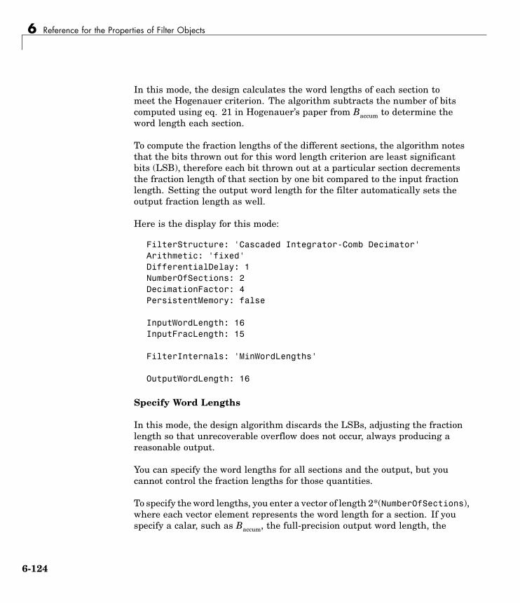
6 Reference for the Properties of Filter Objects
In this mode, the design calculates the word lengths of each section tomeet the Hogenauer criterion. The algorithm subtracts the number of bitscomputed using eq. 21 in Hogenauer’s paper from Baccum to determine theword length each section.
To compute the fraction lengths of the different sections, the algorithm notesthat the bits thrown out for this word length criterion are least significantbits (LSB), therefore each bit thrown out at a particular section decrementsthe fraction length of that section by one bit compared to the input fractionlength. Setting the output word length for the filter automatically sets theoutput fraction length as well.
Here is the display for this mode:
FilterStructure: 'Cascaded Integrator-Comb Decimator'Arithmetic: 'fixed'DifferentialDelay: 1NumberOfSections: 2DecimationFactor: 4PersistentMemory: false
InputWordLength: 16InputFracLength: 15
FilterInternals: 'MinWordLengths'
OutputWordLength: 16
Specify Word Lengths
In this mode, the design algorithm discards the LSBs, adjusting the fractionlength so that unrecoverable overflow does not occur, always producing areasonable output.
You can specify the word lengths for all sections and the output, but youcannot control the fraction lengths for those quantities.
To specify the word lengths, you enter a vector of length 2*(NumberOfSections),where each vector element represents the word length for a section. If youspecify a calar, such as Baccum, the full-precision output word length, the
6-124

Multirate Filter Properties
algorithm expands that scalar to a vector of the appropriate size, applying thescalar value to each section.
The CIC design does not check that the specified word lengths aremonotonically decreasing. There are some cases where the word lengths arenot necessarily monotonically decreasing, for example
hcic=mfilt.cicdecim;hcic.FilterInternals='minwordlengths';hcic.Outputwordlength=14;
which are valid CIC filters but the word lengths do not decrease monotonicallyacross the sections.
Here is the display looks like for the SpecifyWordLengths mode.
FilterStructure: 'Cascaded Integrator-Comb Decimator'Arithmetic: 'fixed'DifferentialDelay: 1NumberOfSections: 2DecimationFactor: 4PersistentMemory: false
InputWordLength: 16InputFracLength: 15
FilterInternals: 'SpecifyWordLengths'
SectionWordLengths: [19 18 18 17]
OutputWordLength: 16
Specify Precision
In this mode, you have full control over the word length and fraction lengthsof all sections and the filter output.
When you elect the SpecifyPrecision mode, you must enter a vector oflength 2*(NumberOfSections) with elements that represent the word lengthfor each section. When you enter a scalar such as Baccum, the CIC algorithmexpands that scalar to a vector of the appropriate size and applies the scalar
6-125

6 Reference for the Properties of Filter Objects
value to each section and the output. The design does not check that thisvector is monotonically decreasing.
Also, you must enter a vector of length 2*(NumberOfSections) with elementsthat represent the fraction length for each section as well. When you entera calar such as Baccum, the design applies scalar expansion as done for theword lengths.
Here is the SpecifyPrecision display.
FilterStructure: 'Cascaded Integrator-Comb Decimator'Arithmetic: 'fixed'DifferentialDelay: 1NumberOfSections: 2DecimationFactor: 4PersistentMemory: false
InputWordLength: 16InputFracLength: 15
FilterInternals: 'SpecifyPrecision'
SectionWordLengths: [19 18 18 17]SectionFracLengths: [14 13 13 12]
OutputWordLength: 16OutputFracLength: 11
FilterStructureReports the type of filter object, such as a decimator or fractional integrator.You cannot set this property — it is always read only and results from yourchoice of mfilt object. Because of the length of the names of multiratefilters, FilterStructure often returns a vector specification for the string.For example, when you use mfilt.firfracinterp to design a filter,FilterStructure returns as [1x49 char].
hm=mfilt.firfracinterp
hm =
6-126

Multirate Filter Properties
FilterStructure: [1x49 char]Numerator: [1x72 double]
RateChangeFactors: [3 2]PersistentMemory: false
States: [24x1 double]
InputOffsetWhen you decimate signals whose length is not a multiple of the decimationfactor M, the last samples — (nM +1) to [(n+1)(M) -1], where n is an integer —are processed and used to track where the filter stopped processing input dataand when to expect the next output sample. If you think of the filtering processas generating an output for a block of input data, InputOffset contains acount of the number of samples in the last incomplete block of input data.
Note InputOffset applies only when you set PersistentMemory to true.Otherwise, InputOffset is not available for you to use.
Two different cases can arise when you decimate a signal:
1 The input signal is a multiple of the filter decimation factor. In this case,the filter processes the input samples and generates output samples for allinputs as determined by the decimation factor. For example, processing99 input samples with a filter that decimates by three returns 33 outputsamples.
2 The input signal is not a multiple of the decimation factor. When thisoccurs, the filter processes all of the input samples, generates outputsamples as determined by the decimation factor, and has one or more inputsamples that were processed but did not generate an output sample.
For example, when you filter 100 input samples with a filter which hasdecimation factor of 3, you get 33 output samples, and 1 sample that didnot generate an output. In this case, InputOffset stores the value 1 afterthe filter run.
InputOffset equal to 1 indicates that, if you divide your input signal intoblocks of data with length equal to your filter decimation factor, the filter
6-127

6 Reference for the Properties of Filter Objects
processed one sample from a new (incomplete) block of data. Subsequentinputs to the filter are concatenated with this single sample to form thenext block of length m.
One way to define the value stored in InputOffset is
InputOffset = mod(length(nx),m)
where nx is the number of input samples in the data set and m is thedecimation factor.
Storing InputOffset in the filter allows you to stop filtering a signal atany point and start over from there, provided that the PersistentMemoryproperty is set to true. Being able to resume filtering after stopping asignal lets you break large data sets in to smaller pieces for filtering. WithPersistentMemory set to true and the InputOffset property in the filter,breaking a signal into sections of arbitrary length and filtering the sectionsis equivalent to filtering the entire signal at once.
xtot=[x,x];
ytot=filter(hm1,xtot)
ytot =
0 -0.0003 0.0005 -0.0014 0.0028 -0.0054 0.0092
reset(hm1); % Clear history of the filter
hm1.PersistentMemory='true';
ysec=[filter(hm1,x) filter(hm1,x)]
ysec =
0 -0.0003 0.0005 -0.0014 0.0028 -0.0054 0.0092
This test verifies that ysec (the signal filtered by sections) is equal to ytot(the entire signal filtered at once).
InterpolationFactorAmount to increase the sampling rate. Interpolation factor for the filter. Itspecifies the amount to increase the input sampling rate. It must be aninteger. Two is the default value. You may use any positive value.
6-128

Multirate Filter Properties
NumberOfSectionsNumber of sections used in the multirate filter. By default multirate filtersuse two sections, but any positive integer works.
OverflowModeThe OverflowMode property is specified as one of the following two stringsindicating how to respond to overflows in fixed-point arithmetic:
• 'saturate' — saturate overflows.
When the values of data to be quantized lie outside of the range of thelargest and smallest representable numbers (as specified by the applicableword length and fraction length properties), these values are quantized tothe value of either the largest or smallest representable value, dependingon which is closest.
• 'wrap' — wrap all overflows to the range of representable values.
When the values of data to be quantized lie outside of the range of thelargest and smallest representable numbers (as specified by the data formatproperties), these values are wrapped back into that range using modulararithmetic relative to the smallest representable number. You can learnmore about modular arithmetic in Fixed-Point Toolbox documentation.
These rules apply to the OverflowMode property.
• Applies to the accumulator and output data only.
• Does not apply to coefficients or input data. These always saturate theresults.
• Does not apply to products. Products maintain full precision at all times.Your filters do not lose precision in the products.
Default value: 'saturate'
Note Numbers in floating-point filters that extend beyond the dynamic rangeoverflow to ±inf.
6-129
6 Reference for the Properties of Filter Objects
PolyphaseAccumThe idea behind PolyphaseAccum and AccumWordLength/AccumFracLengthis to distinguish between the adders that always work in full precision(PolyphaseAccum) from the others [the adders that are controlled by theuser (through AccumWordLength and AccumFracLength) and that mayintroduce quantization effects when you set property FilterInternals toSpecifyPrecision].
Given a product format determined by the input word and fractionlengths, and the coefficients word and fraction lengths, doing full precisionaccumulation means allowing enough guard bits to avoid overflows andunderflows.
Property PolyphaseAccum stores the value that was in the accumulator thelast time your filter ran out of input samples to process. The default value forPolyphaseAccum affects the next output only if PersistentMemory is trueand InputOffset is not equal to 0.
PolyphaseAccum stores data in the format for the filter arithmetic.Double-precision filters store doubles in PolyphaseAccum. Single-precisionfilter store singles in PolyphaseAccum. Fixed-point filters store fi objectsin PolyphaseAccum.
PersistentMemoryDetermine whether the filter states get restored to their starting values foreach filtering operation. The starting values are the values in place when youcreate the filter if you have not changed the filter since you constructed it.PersistentMemory returns to zero any state that the filter changes duringprocessing. States that the filter does not change are not affected.
Determine whether the filter states get restored to their starting values foreach filtering operation. The starting values are the values in place when youcreate the filter object. PersistentMemory returns to zero any state that thefilter changes during processing. States that the filter does not change arenot affected. Defaults to true — the filter retains memory about filteringoperations from one to the next. Maintaining memory lets you filter largedata sets as collections of smaller subsets and get the same result.
xtot=[x,x];
6-130

Multirate Filter Properties
ytot=filter(hm1,xtot)
ytot =
0 -0.0003 0.0005 -0.0014 0.0028 -0.0054 0.0092
reset(hm1); % Clear history of the filter
hm1.PersistentMemory='true';
ysec=[filter(hm1,x) filter(hm1,x)]
ysec =
0 -0.0003 0.0005 -0.0014 0.0028 -0.0054 0.0092
This test verifies that ysec (the signal filtered by sections) is equal to ytot(the entire signal filtered at once).
RateChangeFactorsReports the decimation (m) and interpolation (l) factors for the filter objectwhen you create fractional integrators and decimators, although m and lare used as arguments to both decimators and integrators, applying thesame meaning. Combining these factors as input arguments to the fractionaldecimator or integrator results in the final rate change for the signal.
For decimating filters, the default is [2,3]. For integrators, [3,2].
StatesStored conditions for the filter, including values for the integrator and combsections. m is the differential delay and n is the number of sections in the filter.
About the States of Multirate Filters. In the states property you findthe states for both the integrator and comb portions of the filter, stored in afiltstates object. states is a matrix of dimensions m+1-by-n, with the statesin CIC filters apportioned as follows:
• States for the integrator portion of the filter are stored in the first rowof the state matrix.
• States for the comb portion fill the remaining rows in the state matrix.
In the state matrix, state values are specified and stored in double format.
6-131

6 Reference for the Properties of Filter Objects
States stores conditions for the delays between each interpolator phase, thefilter states, and the states at the output of each phase in the filter, includingvalues for the interpolator and comb states.
The number of states is (lh-1)*m+(l-1)*(lo+mo) where lh is the length of eachsubfilter, and l and m are the interpolation and decimation factors. lo and mo,the input and output delays between each interpolation phase, are integersfrom Euclid’s theorem such that lo*l-mo*m = -1 (refer to the reference for moredetails). Use euclidfactors to get lo and mo for an mfilt.firfracdecimobject.
States defaults to a vector of zeros that has length equal to nstates(hm)
6-132

A
Bibliography
• “Advanced Filters” on page A-1
• “Adaptive Filters” on page A-2
• “Multirate Filters” on page A-2
• “Frequency Transformations” on page A-3
Advanced Filters[1] Antoniou, A., Digital Filters: Analysis, Design, and Applications, SecondEdition, McGraw-Hill, Inc., 1993.
[2] Chirlian, P.M., Signals and Filters, Van Nostrand Reinhold, 1994.
[3] Fliege, N.J., Multirate Digital Signal Processing, John Wiley and Sons,1994.
[4] Jackson, L., Digital Filtering and Signal Processing with MATLABExercises, Third edition, Kluwer Academic Publishers, 1996.
[5] Lapsley, P., J. Bier, A. Sholam, and E.A. Lee, DSP Processor Fundamentals:Architectures and Features, IEEE Press, 1997.
[6] McClellan, J.H., C.S. Burrus, A.V. Oppenheim, T.W. Parks, R.W. Schafer,and H.W. Schuessler, Computer-Based Exercises for Signal Processing UsingMATLAB 5, Prentice-Hall, 1998.
[7] Mayer-Baese, U., Digital Signal Processing with Field Programmable GateArrays, Springer, 2001, refer to the BiQuad block diagram on pp. 126 and theIIR Butterworth example on pp. 140.

A Bibliography
[8] Moler, C., “Floating points: IEEE Standard unifies arithmeticmodel.” Cleve’s Corner, The MathWorks, Inc., 1996. Seehttp://www.mathworks.com/company/newsletter/pdf/Fall96Cleve.pdf.
[9] Oppenheim, A.V., and R.W. Schafer, Discrete-Time Signal Processing,Prentice-Hall, 1989.
[10] Shajaan, M., and J. Sorensen, “Time-Area Efficient Multiplier-FreeRecursive Filter Architectures for FPGA Implementation,” IEEE InternationalConference on Acoustics, Speech, and Signal Processing, 1996, pp. 3269-3272.
Adaptive Filters[1] Hayes, M.H., Statistical Digital Signal Processing and Modeling, JohnWiley and Sons, 1996.
[2] Haykin, S., Adaptive Filter Theory, Third Edition, Prentice-Hall, Inc.,1996.
Multirate Filters[1] Fliege, N.J., Multirate Digital Signal Processing, John Wiley and Sons,1994.
[2] Harris, Fredric J, Multirate Signal Processing for CommunicationSystems, Prentice Hall PTR, 2004.
[3] Hogenauer, E. B., “An Economical Class of Digital Filters for Decimationand Interpolation,” IEEE Transactions on Acoustics, Speech, and SignalProcessing, Vol. ASSP-29, No. 2, April 1981, pp. 155-162.
[4] Lyons, Richard G., Understanding Digital Signal Processing, PrenticeHall PTR, 2004
[5] Mitra, S.K., Digital Signal Processing, McGraw-Hill, 1998.
A-2

Frequency Transformations
[6] Orfanidis, S.J., Introduction to Signal Processing, Prentice-Hall, Inc., 1996.
Frequency Transformations[1] Constantinides, A.G., “Spectral Transformations for Digital Filters,” IEEEProceedings, Vol. 117, No. 8, pp. 1585-1590, August 1970.
[2] Nowrouzian, B., and A.G. Constantinides, “Prototype Reference TransferFunction Parameters in the Discrete-Time Frequency Transformations,”Proceedings 33rd Midwest Symposium on Circuits and Systems, Calgary,Canada, Vol. 2, pp. 1078-1082, August 1990.
[3] Feyh, G., J.C. Franchitti, and C.T. Mullis, “Allpass Filter Interpolation andFrequency Transformation Problem,“ Proceedings 20th Asilomar Conferenceon Signals, Systems and Computers, Pacific Grove, California, pp. 164-168,November 1986.
[4] Krukowski, A., G.D. Cain, and I. Kale, “Custom Designed High-OrderFrequency Transformations for IIR Filters,” 38th Midwest Symposium onCircuits and Systems (MWSCAS’95), Rio de Janeiro, Brazil, August 1995.
A-3

A Bibliography
A-4

B
Examples
Use this list to find examples in the documentation.

B Examples
Using FDATool“Example — Design a Notch Filter” on page 4-4“Example — Quantize Double-Precision Filters” on page 4-19“Example — Change the Quantization Properties of Quantized Filters”on page 4-20“Example — Noise Method Applied to a Filter” on page 4-23“Example — Scale an SOS Filter” on page 4-31“Example — Reorder an SOS Filter” on page 4-40“Example — View the Sections of SOS Filters” on page 4-47“Example — Export Coefficients or Objects to the Workspace” on page 4-53“Example — Exporting as a Text File” on page 4-54“Example — Exporting as a MAT-File” on page 4-55“Example — Import XILINX .COE Files” on page 4-56“Example — Design a Fractional Rate Convertor” on page 4-75“Example — Design a CIC Decimator for 8 Bit Input/Output Data” onpage 4-78“Example — Realize a Filter Using FDATool” on page 4-85
Adaptive Filters“Examples of Adaptive Filters That Use LMS Algorithms” on page 5-15“Example of Adaptive Filter That Uses RLS Algorithm” on page 5-36
B-2

Index
IndexAAccumFracLength 6-20AccumWordLength 6-20adaptfilt object
apply to data 5-14adaptfilt object properties
Algorithm 6-108AvgFactor 6-108BkwdPredErrorPower 6-108BkwdPrediction 6-108Blocklength 6-111Coefficients 6-111ConversionFactor 6-111Delay 6-111DesiredSignalStates 6-111EpsilonStates 6-111ErrorStates 6-111FFTCoefficients 6-111FFTStates 6-112FilteredInputStates 6-112FilterLength 6-112ForgettingFactor 6-112FwdPredErrorPower 6-112FwdPrediction 6-112InitFactor 6-112InvCov 6-113KalmanGain 6-113KalmanGainStates 6-113Offset 6-113OffsetCov 6-113Power 6-113ProjectionOrder 6-114ReflectionCoeffsStep 6-114ResetBeforeFiltering 6-114SecondaryPathCoeffs 6-114SecondaryPathEstimate 6-114SecondaryPathStates 6-114SqrtInvCov 6-115States 6-115StepSize 6-115
SwBlockLength 6-115adaptive filter object 5-14
See also adaptfilt objectadaptive filter properties
SqrtCov 6-114Algorithm 6-108antisymmetricfir 6-54arithmetic
about fixed-point 6-20arithmetic property
double 6-21fixed 6-23single 6-22
AvgFactor 6-108
BBkwdPredErrorPower 6-108BkwdPrediction 6-108Blocklength 6-111
Cchanging quantized filter properties in
FDATool 4-20CoeffAutoScale 6-36CoeffFracLength 6-40Coefficients 6-111CoeffWordLength 6-41context-sensitive help 4-88controls
FDATool 4-9ConversionFactor 6-111convert filters 6-66converting filter structures in FDATool 4-26
DDelay 6-111DenAccumFracLength 6-41DenFracLength 6-42
Index-1

Index
Denominator 6-42DenProdFracLength 6-42DenStateFracLength 6-43DenStateWordLength 6-43design methods 1-6
customize 1-7designing fixed-point multirate filters 4-80designing multirate filters 4-80DesiredSignalStates 6-111df1 6-47df1t 6-49df2 6-50df2t 6-52dfilt properties
arithmetic 6-20direct-form I 6-48
transposed 6-49direct-form II 6-50
transposed 6-52double
property value 6-21dynamic properties 6-5
EEpsilonStates 6-111ErrorStates 6-111exporting quantized filters in FDATool 4-53
FFDATool
about 4-2about importing and exporting filters 4-51about quantization mode 4-7apply option 4-9changing quantized filter properties 4-20context-sensitive help 4-88controls 4-9convert structure option 4-26
converting filter structures 4-26exporting quantized filters 4-53frequency point to transform 4-62getting help 4-88import filter dialog box 4-52importable filter structures 4-51importing filters 4-52original filter type 4-58quantized filter properties 4-10quantizing filters 4-10quantizing reference filters 4-19set quantization parameters dialog 4-10setting properties 4-10specify desired frequency location 4-63switching to quantization mode 4-7transform filters in FDATool 4-64transformed filter type 4-63user options 4-9
FFTCoefficients 6-111FFTStates 6-112filter algorithm 1-6
choosing 1-6filter conversions 6-67filter data 1-10filter design
adaptive 5-1customize algorithm 1-7filter analysis 1-9Filter Object 1-8flow chart 1-2multirate filters in FDATool 4-68process 1-2single-rate filters in FDATool 4-3specification 1-4Specifications Object 1-4
Filter Design and Analysis Tool 4-2See also FDATool
filter design GUIcontext-sensitive help 4-88help about 4-88
Index-2

Index
filter design parameters 1-4filter response 1-4filter sections
specifying 6-67filter structures
about 6-43all-pass lattice 6-59direct-form antisymmetric FIR 6-54direct-form FIR 6-56direct-form I 6-47direct-form I SOS IIR 6-48direct-form I transposed 6-49direct-form I transposed IIR 6-49direct-form II 6-50direct-form II IIR 6-50direct-form II SOS IIR 6-51direct-form II transposed 6-52direct-form II transposed IIR 6-52direct-form symmetric FIR 6-64direct-form transposed FIR 6-57FIR transposed 6-57fixed-point 6-46lattice allpass 6-59lattice AR 6-61lattice ARMA 6-63lattice autoregressive moving average 6-63lattice moving average maximum phase 6-60lattice moving average minimum phase 6-61
FilteredInputStates 6-112filterinternals
fixed-point filter 6-43multirate filter 6-122
FilterLength 6-112filters
converting 6-66exporting as MAT-file 4-55exporting as text file 4-54exporting from FDATool 4-53FIR 6-43getting filter coefficients after exporting 4-54
importing and exporting 4-51importing into FDATool 4-52lattice 6-43state-space 6-43
filters, export as MAT-file 4-55FilterStructure property 6-43finite impulse response
antisymmetric 6-54symmetric 6-64
fir 6-56FIR filters 6-43firt 6-57fixed
arithmetic property value 6-23fixed-point filter properties
AccumFracLength 6-20AccumWordLength 6-20Arithmetic 6-20CastBeforeSum 6-34CoeffAutoScale 6-36CoeffFracLength 6-40CoeffWordLength 6-41DenAccumFracLength 6-41DenFracLength 6-42Denominator 6-42DenProdFracLength 6-42DenStateFracLength 6-43DenStateWordLength 6-43FilterStructure 6-43
fixed-point filter states 6-96fixed-point filter structures 6-46fixed-point filters
dynamic properties 6-5fixed-point multirate filters 4-80ForgettingFactor 6-112fraction length
about 6-30negative number of bits 6-30
frequency point to transform 4-62function for opening FDATool 4-7
Index-3
Index
FwdPredErrorPower 6-112FwdPrediction 6-112
Ggetting filter coefficients after exporting 4-54
Iimport filter dialog box in FDATool 4-52import filter dialog box options 4-52
discrete-time filter 4-52frequency units 4-53
import/export filters in FDATool 4-51importing filters 4-52importing quantized filters in FDATool 4-52InitFactor 6-112InvCov 6-113
KKalmanGain 6-113KalmanGainStates 6-113
Llatcallpass 6-59latcmax 6-60lattice filters
allpass 6-59AR 6-61ARMA 6-63autoregressive 6-61MA 6-61moving average maximum phase 6-60moving average minimum phase 6-61
latticear 6-61latticearma 6-63latticeca 6-60latticema 6-61
Mmultiple sections
specifying 6-67multirate filter states 6-131multirate filters
designing 4-80
Nnegative fraction length
interpret 6-30
Oobject properties
AccumWordLength 6-20Offset 6-113OffsetCov 6-113opening FDATool
function for 4-7options
FDATool 4-9original filter type 4-58
PPersistentMemory 6-114Power 6-113precision 6-31ProjectionOrder 6-114properties
dynamic 6-5FilterStructure 6-43ScaleValues 6-84
Qquantization mode in FDATool 4-7quantized filter properties
changing in FDATool 4-20quantized filters
Index-4

Index
architecture 6-43direct-form FIR 6-56direct-form FIR transposed 6-57direct-form symmetric FIR 6-64finite impulse response 6-57lattice allpass 6-59lattice AR 6-61lattice ARMA 6-63lattice coupled-allpass 6-59lattice MA maximum phase 6-60lattice MA minimum phase 6-61reference filter 6-64scaling 6-84specifying 6-64specifying coefficients for multiple
sections 6-67structures 6-43symmetric FIR 6-54
quantized filters propertiesScaleValues 6-84
quantizing filters in FDATool 4-19
Rrealize data 1-10reference coefficients
specifying 6-64ReflectionCoeffs 6-114ReflectionCoeffsStep 6-114represent numeric data 6-30ResetBeforeFiltering
(PersistentMemory) 6-114
SScaleValues property 6-84
interpreting 6-85scaling
implementing for quantized filters 6-85
quantized filters 6-84second-order sections
normalizing 6-67SecondaryPathCoeffs 6-114SecondaryPathEstimate 6-114SecondaryPathStates 6-114set quantization parameters dialog 4-10setting filter properties in FDATool 4-10single
property value 6-22specifying desired frequency location 4-63SqrtCov 6-114SqrtInvCov 6-115starting FDATool 4-7States 6-115states, fixed-point filter 6-96states, multirate filter 6-131StepSize 6-115SwBlockLength 6-115symmetricfir 6-64
Ttransform filter
frequency point to transform 4-62original filter type 4-58specify desired frequency location 4-63transformed filter type 4-63
transformed filter type 4-63
Uusing adaptfilt objects 5-14using FDATool 4-52
Wword length
about 6-30
Index-5