Figure 1 Realization of the Experiment
82
Transcript of Figure 1 Realization of the Experiment


ii
Certain materials are included under the fair use Exemption of the U.S. Copyright Law and have been
prepared according to the fair use guidelines and are restricted from further use
iii
Abstract
The project focuses on the development of an experiment for an olfactory terrain vehicle localizing
a moving gas source inside an enclosed environment using gas, airflow, and proximity sensors.
The experiment simulates the movement of an unmanned air vehicle (UAV) tracing the source of
a leaking gas from another moving aircraft. A literature review was conducted to aid in the
understanding of technologies and processes that have been used in similar experiments. The main
accomplishments of the project include the selection of major design components such as the gas,
robot, and appropriate gas sensors. Other accomplishments include the design and manufacturing
of a sensor mount as well as the development of a robot motion control algorithm using Matlab
and Simulink code and simulations.
iv
Acknowledgements
We would like to thank the following individuals and organizations for the support they
provided our team. Without them, we would not have been able to achieve what we have during
our time working on this project. Our advisors Professors Michael Demetriou and Nikolaos
Gatsonis have helped guide us through the project process every step of the way. We worked
alongside another MQP group, Christopher Clark, Mitchell Greene, and Madeline Seigle, during
the early stages of the project. Tatiana Egorova, a WPI graduate student, helped us understand the
flow simulations that she and the other group worked on and gave us feedback during our weekly
meetings. Barbara Furhman, an Administrative Assistant in the Mechanical Engineering
Department assisted us in the purchasing of all necessary materials for our project. In research and
purchasing, K-Team Corporation, Road Narrows LLC, CO2 Meter Inc., and Ultimate Plastics were
all very accommodating and provided us with useful information about their products and
distribution methods. Lastly, we would like to thank the entire Worcester Polytechnic Institute
Aerospace Faculty. Over the past four years, they have taught us the material necessary to work
on the project at hand, and gave us feedback and asked questions during our weekly department-
wide meetings.

v
Authorship
Title Page ..................................................................................................................... Anglin, Hunt
Abstract .................................................................................................................................. Anglin
Acknowledgements ....................................................................................................................Hunt
Authorship........................................................................................................ Anglin, Hunt, Myles
Table of Contents ............................................................................................. Anglin, Hunt, Myles
List of Figures ................................................................................................................Hunt, Myles
Chapter 1: Introduction ............................................................ Anglin, Clark, Greene, Hunt, Seigle
Chapter 2: Literature Review ........................................................................... Anglin, Hunt, Myles
Section 2.1....................................................................................................................Myles
Section 2.2.................................................................................................................. Anglin
Section 2.3......................................................................................................................Hunt
Chapter 3: Goals, Objectives, & Approach .............................................................................Myles
Chapter 4: Experiment Design ......................................................................... Anglin, Hunt, Myles
Section 4.1.................................................................................................................. Anglin
Section 4.2 .....................................................................................................................Hunt
Section 4.3........................................................................................................ Anglin, Hunt
Section 4.4 ...................................................................................................................Myles
Section 4.5.......................................................................................................... Hunt, Myles
Section 4.6....................................................................................................................Myles
Chapter 5: Results ....................................................................................................................Myles
Chapter 6: Recommendations ..................................................................................................Myles
Appendices ....................................................................................................... Anglin, Hunt, Myles
All members participated in the revising and editing of all chapters of the report.
All photos are by the authors unless otherwise noted.

vi
Table of Contents Abstract .............................................................................................................................. iii
Acknowledgements ............................................................................................................ iv
Authorship........................................................................................................................... v
List of Figures ................................................................................................................... vii
1 Introduction ................................................................................................................... 1
1.1 Overview .................................................................................................................... 1
1.2 Research ..................................................................................................................... 2
1.3 Goals .......................................................................................................................... 3
1.4 Robot Research and Selection ................................................................................... 3
1.5 Gas Sensor Research and Selection ........................................................................... 4
1.6 Wind Sensor Research ............................................................................................... 5
1.7 External Chassis Design ............................................................................................ 5
1.8 Motion Control and Simulations ............................................................................... 5
2 Literature Review.......................................................................................................... 7
2.1 Multiple Gas Sensing Localization Experiment ........................................................ 7
2.2 Swarm Robot Navigation Experiment ..................................................................... 10
2.3 Gas Distribution Experiments for Inspection by Mobile Robots ............................ 12
3 Goals, Objectives & Approach ................................................................................... 16
4 Experiment Design...................................................................................................... 17
4.1 Robot Selection ........................................................................................................ 17
4.2 Gas Sensor Selection ............................................................................................... 21
4.3 Wind Sensor Selection ............................................................................................. 23
4.4 External Chassis ....................................................................................................... 28
4.5 Price, Weight, and Power Budgets .......................................................................... 33
4.6 Motion Control/Navigation...................................................................................... 34
4.6.1 Control Modes ............................................................................................... 34
4.6.2 Kinematic Motion Study ............................................................................... 37
4.6.3 Simulations .................................................................................................... 44
5 Results ......................................................................................................................... 47
6 Conclusions and Recommendations ........................................................................... 49
6.1 Conclusions .............................................................................................................. 49
6.2 Recommendations .................................................................................................... 50
References ......................................................................................................................... 52
Appendix A : APM 2.6 Airspeed Sensor Kit, Airspeed Error .......................................... 54
Appendix B : Sensor Mount Drawings ............................................................................. 55
Appendix C : Sensor Mount Static Stress Analysis .......................................................... 57
Appendix D : Simulink Robot Control Code .................................................................... 60
Appendix E : V-rep Simulation Code ............................................................................... 66

vii
List of Figures
Figure 1 Realization of the Experiment 1
Figure 2 Plume Generation and Detection Experiment 2
Figure 3 The E-nose used in the Martinez, Rochel, Hugues experiment 7
Figure 4 Koala robot setup from the Martinez, Rochel, Hugues experiment 8
Figure 5 The experimental setup for the Martinez, Rochel, Hugues experiment 8
Figure 6 Successful trajectories from the Martinez, Rochel, Hugues experiment 9
Figure 7 A swarm of robots moving toward the odor source 10
Figure 8 Cooperative localization system; three stationary beacons and one robot moving 11
Figure 9 Khepera III and KheNose with sensing modules 11
Figure 10 Two Erratic and two Khepera III robots localizing the odor source 12
Figure 11 ATRV Robot Setup 13
Figure 12 Koala Robot Setup 14
Figure 13 Results of Tubingen Experiment 15
Figure 14 Results of Orebro Experiment 15
Figure 15 ATRV junior and specifications 18
Figure 16 ATRV experimental setup 18
Figure 17 Koala 2.5 and specifications 19
Figure 18 Korebot II and the KoreIO extension board 19
Figure 19 Khepera III and specifications 20
Figure 20 Khepera IV and specifications 21
Figure 21 COZIR Ambient 10k CO2 Sensor 22
Figure 22 CAD Model of the COZIR Ambient 10K Sensor 23
Figure 23 DS-2 Sonic Anemometer 24
Figure 24 FT702LM OEM Airflow Sensor 24
Figure 25 T-DCI-F900-S-P Airflow Sensor 25
Figure 26 PCB-RFS300 25
Figure 27 F600 Series PCB 26
Figure 28 APM 2.6 Airspeed Sensor Kit 26
Figure 29 APM 2. Airspeed Sensor connected to a board 27
Figure 30 Pitot tube assembled at nose of UAV 27
Figure 31 M3 screw positioning 28
Figure 32 Preliminary mount design 29
Figure 33 Updated mount design with assembly 30

viii
Figure 34 Updated Design for metal mount 31
Figure 35 Updated Sensor Mount Design 32
Figure 36 Budget Chart 33
Figure 37 Speed profile control example 35
Figure 38 An example of position control 36
Figure 39 Main Simulink model 40
Figure 40 Desired x and y positions 41
Figure 41 Actual x and y positions 42
Figure 42 Perterbation from x and y desired in circular model 43
Figure 43 Values given by the atan2 of y and x velocities over time 43
Figure 44 Final simulation run for the half parabola shape 44
Figure 45 Final shape generated by the V-rep software using the data for the half parabola simulation 46
1
1 Introduction
1.1 Overview
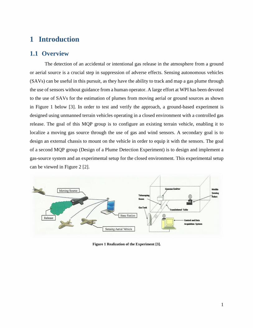
The detection of an accidental or intentional gas release in the atmosphere from a ground
or aerial source is a crucial step in suppression of adverse effects. Sensing autonomous vehicles
(SAVs) can be useful in this pursuit, as they have the ability to track and map a gas plume through
the use of sensors without guidance from a human operator. A large effort at WPI has been devoted
to the use of SAVs for the estimation of plumes from moving aerial or ground sources as shown
in Figure 1 below [3]. In order to test and verify the approach, a ground-based experiment is
designed using unmanned terrain vehicles operating in a closed environment with a controlled gas
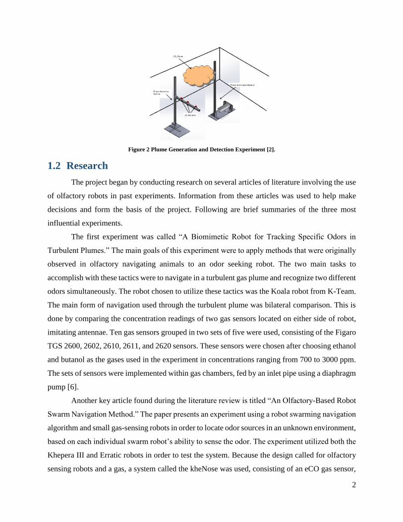
release. The goal of this MQP group is to configure an existing terrain vehicle, enabling it to
localize a moving gas source through the use of gas and wind sensors. A secondary goal is to
design an external chassis to mount on the vehicle in order to equip it with the sensors. The goal
of a second MQP group (Design of a Plume Detection Experiment) is to design and implement a
gas-source system and an experimental setup for the closed environment. This experimental setup
can be viewed in Figure 2 [2].
Figure 1 Realization of the Experiment [3].
2
Figure 2 Plume Generation and Detection Experiment [2].
1.2 Research
The project began by conducting research on several articles of literature involving the use
of olfactory robots in past experiments. Information from these articles was used to help make
decisions and form the basis of the project. Following are brief summaries of the three most
influential experiments.
The first experiment was called “A Biomimetic Robot for Tracking Specific Odors in
Turbulent Plumes.” The main goals of this experiment were to apply methods that were originally
observed in olfactory navigating animals to an odor seeking robot. The two main tasks to
accomplish with these tactics were to navigate in a turbulent gas plume and recognize two different
odors simultaneously. The robot chosen to utilize these tactics was the Koala robot from K-Team.
The main form of navigation used through the turbulent plume was bilateral comparison. This is
done by comparing the concentration readings of two gas sensors located on either side of robot,
imitating antennae. Ten gas sensors grouped in two sets of five were used, consisting of the Figaro
TGS 2600, 2602, 2610, 2611, and 2620 sensors. These sensors were chosen after choosing ethanol
and butanol as the gases used in the experiment in concentrations ranging from 700 to 3000 ppm.
The sets of sensors were implemented within gas chambers, fed by an inlet pipe using a diaphragm
pump [6].
Another key article found during the literature review is titled “An Olfactory-Based Robot
Swarm Navigation Method.” The paper presents an experiment using a robot swarming navigation
algorithm and small gas-sensing robots in order to locate odor sources in an unknown environment,
based on each individual swarm robot’s ability to sense the odor. The experiment utilized both the
Khepera III and Erratic robots in order to test the system. Because the design called for olfactory
sensing robots and a gas, a system called the kheNose was used, consisting of an eCO gas sensor,
3
three thermal anemometers and two eNostril sensors for each robot. In order to track the
movements of the swarm, individual robots took turns acting as stationary beacons while the others
moved, using the Zigbee network to communicate with each other. After several trials of this setup
using four robots, the system appeared to be a success. All of the robots were able to move to the
gas source in the test runs, with some variances. In general, the tests would take longer if the air
flow in the environment was stronger, as well as if the sensors received large changes in
concentrations [5].
A third experiment highlighted is called “Gas Distribution in Unventilated Indoor
Environments Inspected by a Mobile Robot,” which analyzed the results of two identical tests
conducted in Tubingen, Germany and Orebro, Sweden. The tests were designed to analyze the
results of gas distribution in unventilated environments if patrolled by fixed-course olfactory
robots. The robots used in the experiments were the ATRV and the Koala Bot, made by iRobot
and K-Team respectively. The gas sensors used on the ATRV were the TGS 2620 gas sensors,
placed vertically from one another to measure different heights. The TGS 2600, 2610, and 2620
sensors were placed on the Koala Bot. The analysis tests with each robot were ran twice, once in
the summer and once in the winter. The report shows that the tests had similar results during the
different times of the year [4].
1.3 Goals
The goal of the project is to work in conjunction with another group to set up an
experiment that would allow a gas sensing terrain vehicle to localize a gas source and reconstruct
the gas plume. In order to achieve this, a robot that could read and send sensor data wirelessly
needed to be selected. Next, gas sensors that could send gas concentration data to a computer
base station had to be chosen. A mount for the sensors also had to be created so that they could
be attached to the robot. These sensors required a data acquisition system to collect and log data
to use for the robot’s motion. Finally, to keep track of the robot’s motion, a guidance and
navigation system needed to be designed to model the motion during the experiment as well as
during simulations beforehand.
1.4 Robot Research and Selection
After conducting a literature review, there was extensive research into the robots used in
similar types of experiments. The robot needed for this experiment had several requirements. The

4
first requirement was a small, compact size that would minimize the effect it would have on the
air flow while moving. The robot also had to be able to support enough weight for four gas sensors,
and an anemometer. It would also need to be able to connect wirelessly with a base station to
communicate its readings and receive movement commands.
From the conducted research and literature reviews, three robots appeared viable: the
ATRV-Jr, the Koala Bot, and the Khepera III. The third option, the Khepera III, is made by K-
Team. It is a small mobile robot, 13cm in diameter and 7cm in height. It reaches a maximum speed
of 0.5m/s and weighs approximately 690g, with a payload of 2000g. It requires a Korebot II board
and KoreIO extension board in order to add external sensors. The Khepera III communicates
wirelessly via Korebot Wireless Ethernet. It also includes several proximity sensors, both infrared
and ultrasonic, with a range of 20cm to 4m [7].
After researching all three robots, the Khepera III was selected. Road Narrows LLC, the
North American K-Team Distributer, was then contacted about receiving a quote and
determining other logistics. They announced that the Khepera IV was about to be released and
released the specifications sheet. The Khepera IV was an upgraded version of the Khepera III
and turned out to fit the needs of the project even better [1].
1.5 Gas Sensor Research and Selection
Moving forward, the next step was to determine a setup for the gas sensors to be placed on
the Khepera IV. The design constraints for the project required four gas sensors located at the
front, back, and sides of the robot, two feet apart from one another. Because this experiment
requires an olfactory robot, the COZIR Ambient 10K CO2 Sensor produced by CO2 Meter was
selected, once it was established by the other MQP group NAG1501 that the choice of gas was
CO2. The gas sensor parameters considered when making this selection included a low power
need, low response time, high accuracy, appropriate measurement range, and a high measurement
frequency. The power need of each sensor is 3.5mW, which is ultra-low compared to the output
of the Khepera IV robot. A low response time of the gas sensor ensures that the sensor is making
measurements that represent the environment’s actual local levels. The COZIR sensors were the
best match for this, sitting at less than 3 seconds in response time. It has an accuracy of ±50 ppm
+/- 3% of the reading which should be low enough for this application. The sensor has a
measurement range from 0-10,000 ppm, which should fit this experiment. The sensor is also

5
capable of making individual measurements every 0.5 seconds. This is one of the highest
measurement frequencies for a CO2 sensor that was found.
1.6 Wind Sensor Research
From the beginning of the project, it had been noted that finding an appropriate wind
sensor could help the algorithm for gas source localization. For the duration of the project, most
of the airspeed sensors found would neither fit on the Khepera IV nor fit the needs of the project.
Wind sensors that require the input of a differential pressure sensor from a Prandtl tube would be
ideal for a UAV application. However, after some calculations for error analysis which was done
for pitot tube sensor APM 2.6 Airspeed Sensor using Microsoft Excel, the setup propagates too
much error to be utilized due to the low operational speeds of the Khepera IV. Appendix A
shows the results of these calculations.
1.7 External Chassis Design
Over the course of the project, a series of designs for a sensor mount were developed. The
mount needed to extend a distance of 1 foot from the center of the robot in the shape of a cross,
disturbing airflow as little as possible. The mount’s weight also needed to be minimized to ensure
that the Khepera IV can handle the payload while still moving as desired. For the final design, two
pieces of acrylic were cut 8 inches in length and were placed perpendicular to each other such that
the holes in the center of each were cut to be secured to the robot with M3 spacers and screws.
This design resulted in the final weight of the mount at 564.66 grams, meeting the robot’s payload
limit of 2 kg. The design’s detailed drawings are provided in Appendix B. The acrylic was easily
purchased and cut using the WPI Machine Lab’s Laser Cutter.
1.8 Motion Control and Simulations
The motion of the Khepera IV can be controlled with four different control modes that are
built into the robot. Speed control mode was the main focus for the simulations because it was the
most simple to replicate with the given software. In this mode, the robot takes a velocity command
for each wheel and tries to accelerate the wheels to their respective velocities as quickly as
possible. The velocity command ranges from 5 to 1,200 which correspond to a real velocity of 3
mm/s to 813 mm/s. To obtain the real values, the velocity command must be multiplied by
6
0.678181, a factor determined by the geometric properties of the Khepera IV. The minimum value
for the velocity is determined by the PID controller, which is active in speed control mode [1].
With an understanding of the different control options for the robot, the goal was to create
a kinematic model that would simulate the robot’s motion based on speed control mode. The
kinematic equations that dictate the motion were determined with some research and basic math.
A simulation model was created in Simulink software to test these equations. This model created
an artificial path for the robot to follow based on parametric equations. The parametric equations
were x and y positions as a function of time. The derivatives of these functions were then taken to
determine the x and y velocities as a function of time. For this experiment, the gas sensor
concentrations would determine the x and y velocities for the robot. The x and y velocities are then
run through a set of control laws which determine the input to the robot. The Simulink model then
takes these values and sets up the kinematic differential equations of motion. These are then solved
to determine the actual x and y positions of the robot. Since the desired x and y positions are known
in the model from the parametric equations, the actual position of the robot could be compared to
the desired position.
The Simulink model also generates the angular velocities of each wheel, as this is the true
input to the robot. These angular velocities could be used in a simulation software provided by
K-Team for robot called V-rep. This software has a three dimensional visual representation of
the robot and allows the control of the robot using the LUA programming language. Since the
Khepera IV is a new model, the only model available in V-rep is the Khepera III. Two
simulations were worked throughout the duration of the project. The first simulation was a very
basic algorithm that adjusted the robot’s motion based on simulated gas sensors. The gas sensors
in the program generated random gas concentrations. When the concentration on one side of the
robot was higher than another side, the robot would move towards that side. This simulation also
made use of the robot’s infrared proximity sensors. If the robot was too close to a wall, then the
proximity sensors would be triggered and the robot would turn around. The second simulation
made use of the Simulink model. It took the angular velocities for each wheel that was generated
by the model and applied it to the robot at given time intervals. After some debugging of both the
Simulink and V-rep codes, a model was achieved that depicted the desired motion.
7
2 Literature Review
The project began with the research of numerous articles of literature depicting past
experiments involving the use of olfactory robots. Information was used from these articles to help
make decisions and form the basis of the project. Following are brief summaries of the three most
influential experiments.
2.1 Multiple Gas Sensing Localization Experiment
The first case researched was an experiment very similar to this project. This experiment
was carried out by Dominique Martinez, Oliver Rochel, and Etienne Hugues. Their findings are
outlined in a research paper titled “A Biomimetic Robot for Tracking Specific Odors in Turbulent
Plumes” [6]. The main goals of this experiment were to employ tactics that were originally
observed in animals to an odor seeking robot. The two main tasks were to have the robot navigate
in a turbulent plume and recognize two odors simultaneously. To navigate in a turbulent plume,
the group planned on using bilateral comparison. This is when there are two sensors on either side
of the odor seeking device and the concentration of gas can be monitored at each side of the device.
Then, by comparing the two concentration readings, the robot decides to maneuver accordingly.
This is similar to how some insects have two antennae to sense different odors simultaneously.
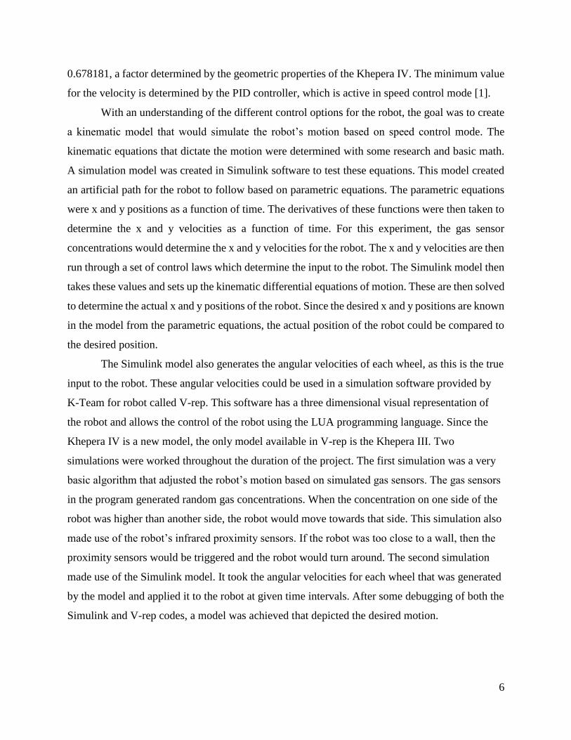
For this experiment, the Koala robot from K-team was used. “E-noses” were attached to
both sides of the robot. These are sensor arrays with ten gas sensors in each configuration, placed
in a small Plexiglas chamber. The ten gas sensors consisted of two each of the Figaro TGS 2600,
2602, 2610, 2611, and 2620.
Figure 3 The E-nose used in the Martinez, Rochel, Hugues experiment [6].
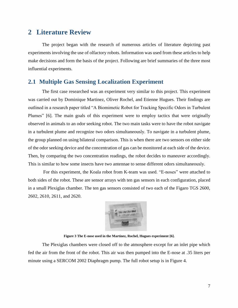
The Plexiglas chambers were closed off to the atmosphere except for an inlet pipe which
fed the air from the front of the robot. This air was then pumped into the E-nose at .35 liters per
minute using a SERCOM 2002 Diaphragm pump. The full robot setup is in Figure 4.
8
Figure 4 Koala robot setup from the Martinez, Rochel, Hugues experiment [6].
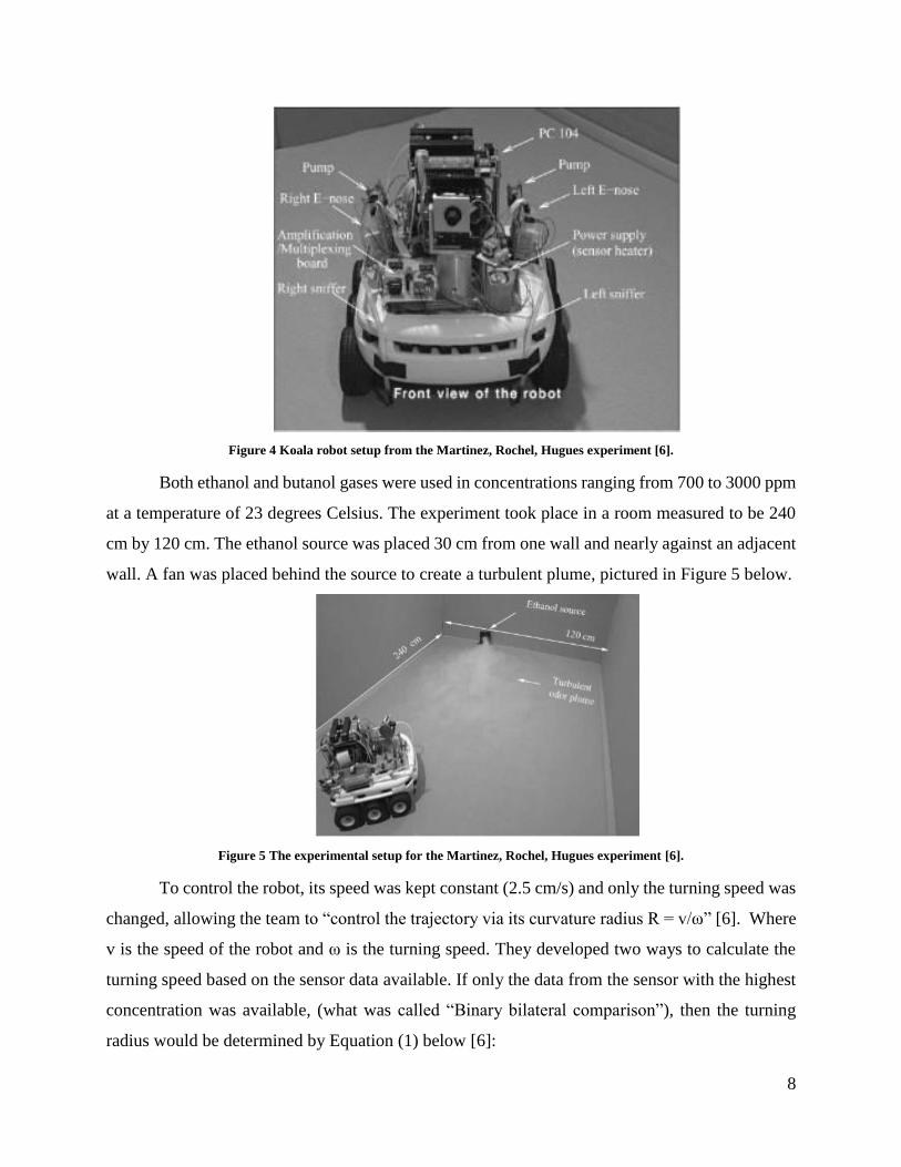
Both ethanol and butanol gases were used in concentrations ranging from 700 to 3000 ppm
at a temperature of 23 degrees Celsius. The experiment took place in a room measured to be 240
cm by 120 cm. The ethanol source was placed 30 cm from one wall and nearly against an adjacent
wall. A fan was placed behind the source to create a turbulent plume, pictured in Figure 5 below.
Figure 5 The experimental setup for the Martinez, Rochel, Hugues experiment [6].
To control the robot, its speed was kept constant (2.5 cm/s) and only the turning speed was
changed, allowing the team to “control the trajectory via its curvature radius R = v/ω” [6]. Where
v is the speed of the robot and ω is the turning speed. They developed two ways to calculate the
turning speed based on the sensor data available. If only the data from the sensor with the highest
concentration was available, (what was called “Binary bilateral comparison”), then the turning
radius would be determined by Equation (1) below [6]:
9
𝜔(𝑡) = Ω(𝑡) ∗ sgn ∆𝐶(𝑡) (1)
Where ∆𝐶 is the change in concentration, t is time, and Ω(𝑡) is some turning speed. If the
team had access to graded information from both sensors, (called “analog bilateral comparison”)
then the turning speed would be determined by Equation (2) below [6]:
𝜔(𝑡) = Ω0 ∗ sgn ∆𝐶(𝑡) ∗ |∆𝐶(𝑡)|𝑛 ∗ 𝑐1−2𝑛 (2)
Where 𝑐 is the average concentration (both concentrations added up and divided by two)
and the rest of the parameters are the same from the previous equation.
These calculations do not depend on the wind. Anemometers were not used because
“relative imprecision of the anemometers that can be used on real robots” makes this approach
only valid “in presence of a strong airflow” [6].
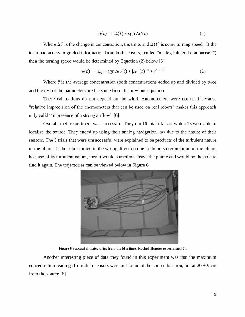
Overall, their experiment was successful. They ran 16 total trials of which 13 were able to
localize the source. They ended up using their analog navigation law due to the nature of their
sensors. The 3 trials that were unsuccessful were explained to be products of the turbulent nature
of the plume. If the robot turned in the wrong direction due to the misinterpretation of the plume
because of its turbulent nature, then it would sometimes leave the plume and would not be able to
find it again. The trajectories can be viewed below in Figure 6.
Figure 6 Successful trajectories from the Martinez, Rochel, Hugues experiment [6].
Another interesting piece of data they found in this experiment was that the maximum
concentration readings from their sensors were not found at the source location, but at 20 ± 9 cm
from the source [6].
10
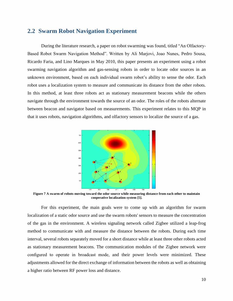
2.2 Swarm Robot Navigation Experiment
During the literature research, a paper on robot swarming was found, titled “An Olfactory-
Based Robot Swarm Navigation Method”. Written by Ali Marjovi, Joao Nunes, Pedro Sousa,
Ricardo Faria, and Lino Marques in May 2010, this paper presents an experiment using a robot
swarming navigation algorithm and gas-sensing robots in order to locate odor sources in an
unknown environment, based on each individual swarm robot’s ability to sense the odor. Each
robot uses a localization system to measure and communicate its distance from the other robots.
In this method, at least three robots act as stationary measurement beacons while the others
navigate through the environment towards the source of an odor. The roles of the robots alternate
between beacon and navigator based on measurements. This experiment relates to this MQP in
that it uses robots, navigation algorithms, and olfactory sensors to localize the source of a gas.
Figure 7 A swarm of robots moving toward the odor source while measuring distance from each other to maintain
cooperative localization system [5].
For this experiment, the main goals were to come up with an algorithm for swarm
localization of a static odor source and use the swarm robots' sensors to measure the concentration
of the gas in the environment. A wireless signaling network called Zigbee utilized a leap-frog
method to communicate with and measure the distance between the robots. During each time
interval, several robots separately moved for a short distance while at least three other robots acted
as stationary measurement beacons. The communication modules of the Zigbee network were
configured to operate in broadcast mode, and their power levels were minimized. These
adjustments allowed for the direct exchange of information between the robots as well as obtaining
a higher ratio between RF power loss and distance.
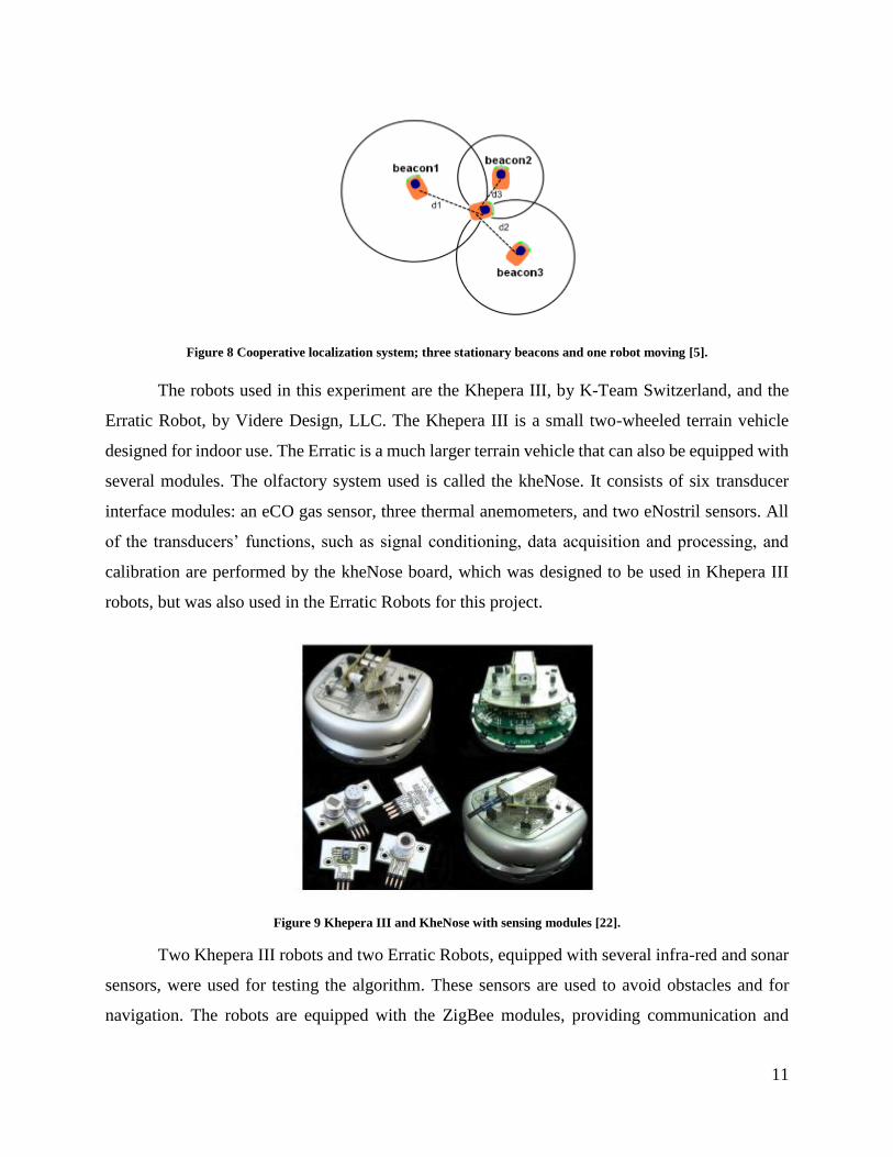
11
Figure 8 Cooperative localization system; three stationary beacons and one robot moving [5].
The robots used in this experiment are the Khepera III, by K-Team Switzerland, and the
Erratic Robot, by Videre Design, LLC. The Khepera III is a small two-wheeled terrain vehicle
designed for indoor use. The Erratic is a much larger terrain vehicle that can also be equipped with
several modules. The olfactory system used is called the kheNose. It consists of six transducer
interface modules: an eCO gas sensor, three thermal anemometers, and two eNostril sensors. All
of the transducers’ functions, such as signal conditioning, data acquisition and processing, and
calibration are performed by the kheNose board, which was designed to be used in Khepera III
robots, but was also used in the Erratic Robots for this project.
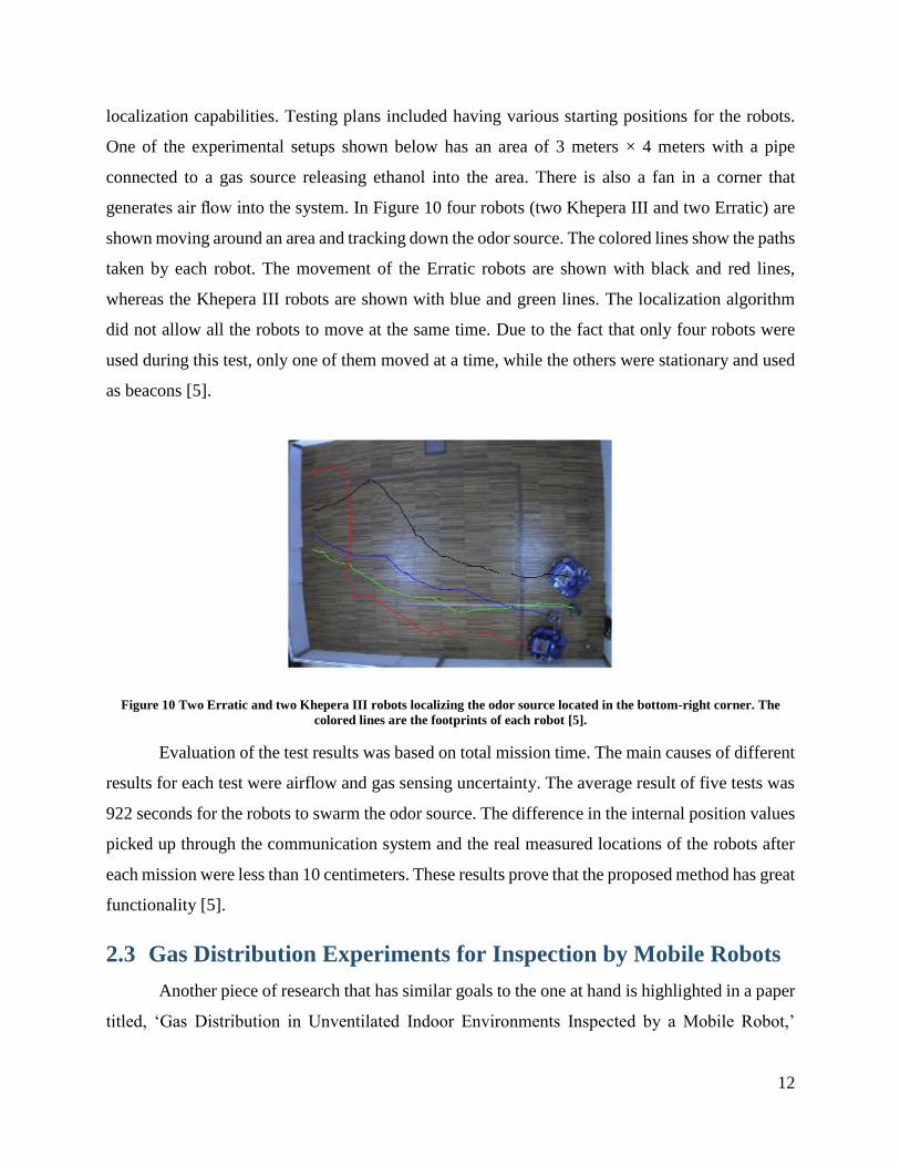
Figure 9 Khepera III and KheNose with sensing modules [22].
Two Khepera III robots and two Erratic Robots, equipped with several infra-red and sonar
sensors, were used for testing the algorithm. These sensors are used to avoid obstacles and for
navigation. The robots are equipped with the ZigBee modules, providing communication and
12
localization capabilities. Testing plans included having various starting positions for the robots.
One of the experimental setups shown below has an area of 3 meters × 4 meters with a pipe
connected to a gas source releasing ethanol into the area. There is also a fan in a corner that
generates air flow into the system. In Figure 10 four robots (two Khepera III and two Erratic) are
shown moving around an area and tracking down the odor source. The colored lines show the paths
taken by each robot. The movement of the Erratic robots are shown with black and red lines,
whereas the Khepera III robots are shown with blue and green lines. The localization algorithm
did not allow all the robots to move at the same time. Due to the fact that only four robots were
used during this test, only one of them moved at a time, while the others were stationary and used
as beacons [5].
Figure 10 Two Erratic and two Khepera III robots localizing the odor source located in the bottom-right corner. The
colored lines are the footprints of each robot [5].
Evaluation of the test results was based on total mission time. The main causes of different
results for each test were airflow and gas sensing uncertainty. The average result of five tests was
922 seconds for the robots to swarm the odor source. The difference in the internal position values
picked up through the communication system and the real measured locations of the robots after
each mission were less than 10 centimeters. These results prove that the proposed method has great
functionality [5].
2.3 Gas Distribution Experiments for Inspection by Mobile Robots
Another piece of research that has similar goals to the one at hand is highlighted in a paper
titled, ‘Gas Distribution in Unventilated Indoor Environments Inspected by a Mobile Robot,’
13
which was conducted in both Tubingen, Germany and Orebro, Sweden with two different but
similar setups. In this paper, both teams attempt odor localization of a gas source in an unventilated
room using mobile, olfactory robots. Typically, experiments including gas localization are
completed in environments with a strong uni-directional air flow. In order to confirm the test
results, the experiments were performed in both summer and winter, when convection and heat
flows vary.
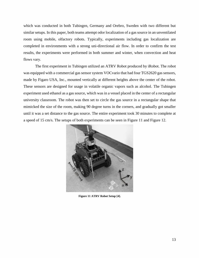
The first experiment in Tubingen utilized an ATRV Robot produced by iRobot. The robot
was equipped with a commercial gas sensor system VOCvario that had four TGS2620 gas sensors,
made by Figaro USA, Inc., mounted vertically at different heights above the center of the robot.
These sensors are designed for usage in volatile organic vapors such as alcohol. The Tubingen
experiment used ethanol as a gas source, which was in a vessel placed in the center of a rectangular
university classroom. The robot was then set to circle the gas source in a rectangular shape that
mimicked the size of the room, making 90 degree turns in the corners, and gradually got smaller
until it was a set distance to the gas source. The entire experiment took 30 minutes to complete at
a speed of 15 cm/s. The setups of both experiments can be seen in Figure 11 and Figure 12.
Figure 11 ATRV Robot Setup [4].
14
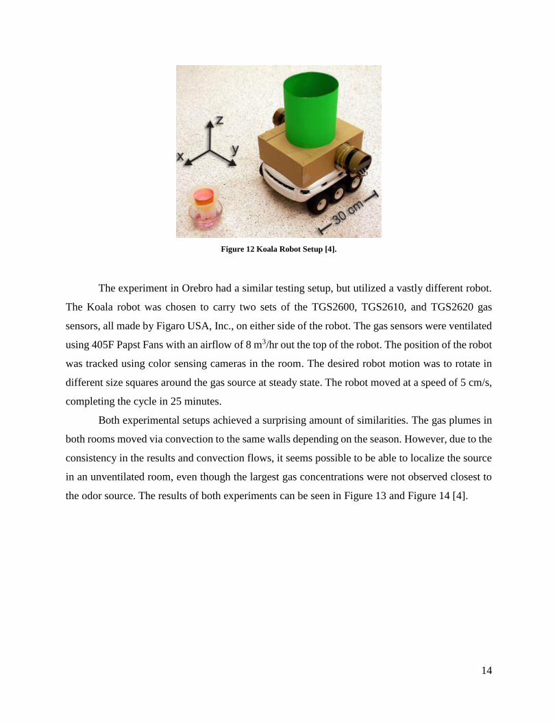
Figure 12 Koala Robot Setup [4].
The experiment in Orebro had a similar testing setup, but utilized a vastly different robot.
The Koala robot was chosen to carry two sets of the TGS2600, TGS2610, and TGS2620 gas
sensors, all made by Figaro USA, Inc., on either side of the robot. The gas sensors were ventilated
using 405F Papst Fans with an airflow of 8 m3/hr out the top of the robot. The position of the robot
was tracked using color sensing cameras in the room. The desired robot motion was to rotate in
different size squares around the gas source at steady state. The robot moved at a speed of 5 cm/s,
completing the cycle in 25 minutes.
Both experimental setups achieved a surprising amount of similarities. The gas plumes in
both rooms moved via convection to the same walls depending on the season. However, due to the
consistency in the results and convection flows, it seems possible to be able to localize the source
in an unventilated room, even though the largest gas concentrations were not observed closest to
the odor source. The results of both experiments can be seen in Figure 13 and Figure 14 [4].

15
Figure 13 Results of Tubingen Experiment [4].
Figure 14 Results of Orebro Experiment [4].
16
3 Goals, Objectives & Approach
The main goal of this project is to work in conjunction with another MQP group to set up an
experiment that would allow a gas sensing terrain vehicle to localize a gas source and then
reconstruct the gas plume. To reach this goal, there are also several sub goals. First and foremost
is to choose a robotic vehicle capable of fulfilling the project needs. The robot needs to be able to
read and send sensor data wirelessly; otherwise, a separate system will need to be designed to do
so. Next, the gas sensors have to be selected. Based on the gas source collaboratively selected by
both MQP groups, a gas sensor will be chosen that will send gas concentration data to the base
station. An air flow sensor may also be selected so that wind data could be added to the algorithm
that determines the robot’s motion. Depending on the robot selection, an external mount for the
sensors may be created, which will be attached on top of the robot. These sensors will also require
a data acquisition system to collect and log data for the robot to use. Finally, to keep track of the
robot’s motion, a guidance and navigation system will be developed. This system will be used to
both model the robot’s motion during the experiment and to simulate the motion beforehand.
The robot and sensor selection will be completed with research from literature reviews as
well as extended research on individual products. The motion control algorithm will be done in
either Matlab or Simulink. Both research and analysis will help create this algorithm. CAD files
will be created to model the entire system using SolidWorks, for better visualization of the
experiment. The CAD software will also be used to design the external mount for the sensors,
which will then need to be manufactured. When the experiment runs, the gas sensors will collect
readings of gas concentrations which will be used to recreate the gas plume using computer
software.
17
4 Experiment Design
In the following sections, the process of selecting a robot, gas sensor, and anemometer for
the project were discussed, as well as the designing process for an external mount located on top
of the robot. The modes of motion control, kinematic motion study, and simulations that were used
to configure the robot’s motion and navigation are also discussed.
4.1 Robot Selection
This project required a small to medium sized mobile robot. The experiment would be
performed in a completely enclosed area. The area would be built indoors and be approximately
10m by 10m with a height of 3m. The entire robot also had to be smaller than the plume of CO2
gas used in the enclosed area. Other requirements are that the robot must have the correct extension
modules for the equipment of four CO2gas sensors and at least one anemometer, as well as a
wireless communication method and motion control.
From the background research and literature reviews, the robot options were narrowed
down to three: ATRV-Jr, Koala Bot, and Khepera III. The ATRV-Jr is a four-wheeled mobile
robot with differential steering, zero turn radius, and a maximum speed of 1m/s. Its dimensions
are 77.5cm by 55cm and weighs 50kg (110 lbs). It has a weight payload of 25kg (55.1lbs) and uses
wireless communication by either RS-232 or Ethernet.
18
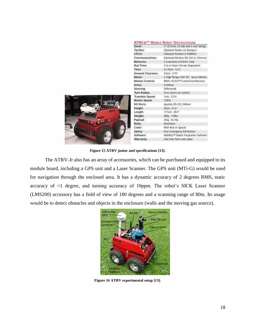
Figure 15 ATRV junior and specifications [13].
The ATRV-Jr also has an array of accessories, which can be purchased and equipped to its
module board, including a GPS unit and a Laser Scanner. The GPS unit (MTi-G) would be used
for navigation through the enclosed area. It has a dynamic accuracy of 2 degrees RMS, static
accuracy of <1 degree, and turning accuracy of 10ppm. The robot’s SICK Laser Scanner
(LMS200) accessory has a field of view of 180 degrees and a scanning range of 80m. Its usage
would be to detect obstacles and objects in the enclosure (walls and the moving gas source).
Figure 16 ATRV experimental setup [13].
19
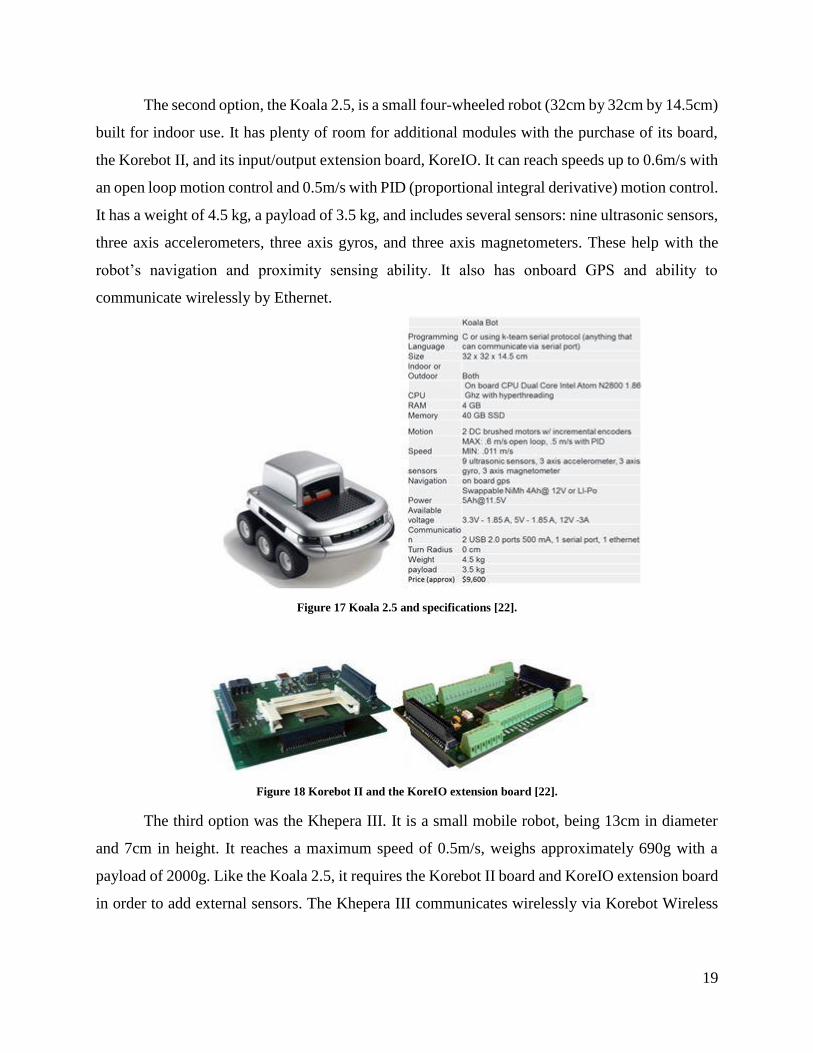
The second option, the Koala 2.5, is a small four-wheeled robot (32cm by 32cm by 14.5cm)
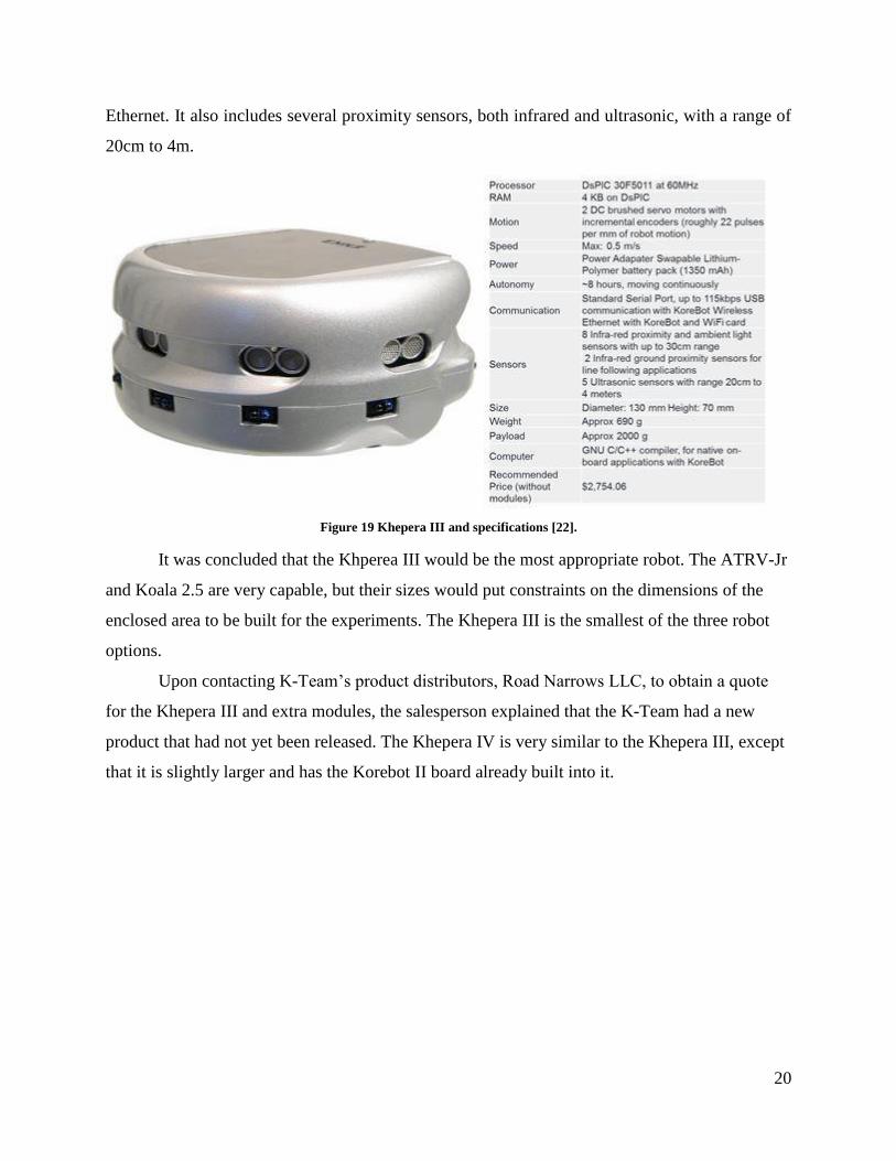
built for indoor use. It has plenty of room for additional modules with the purchase of its board,
the Korebot II, and its input/output extension board, KoreIO. It can reach speeds up to 0.6m/s with
an open loop motion control and 0.5m/s with PID (proportional integral derivative) motion control.
It has a weight of 4.5 kg, a payload of 3.5 kg, and includes several sensors: nine ultrasonic sensors,
three axis accelerometers, three axis gyros, and three axis magnetometers. These help with the
robot’s navigation and proximity sensing ability. It also has onboard GPS and ability to
communicate wirelessly by Ethernet.
Figure 17 Koala 2.5 and specifications [22].
Figure 18 Korebot II and the KoreIO extension board [22].
The third option was the Khepera III. It is a small mobile robot, being 13cm in diameter
and 7cm in height. It reaches a maximum speed of 0.5m/s, weighs approximately 690g with a
payload of 2000g. Like the Koala 2.5, it requires the Korebot II board and KoreIO extension board
in order to add external sensors. The Khepera III communicates wirelessly via Korebot Wireless
20
Ethernet. It also includes several proximity sensors, both infrared and ultrasonic, with a range of
20cm to 4m.
Figure 19 Khepera III and specifications [22].
It was concluded that the Khperea III would be the most appropriate robot. The ATRV-Jr
and Koala 2.5 are very capable, but their sizes would put constraints on the dimensions of the
enclosed area to be built for the experiments. The Khepera III is the smallest of the three robot
options.
Upon contacting K-Team’s product distributors, Road Narrows LLC, to obtain a quote
for the Khepera III and extra modules, the salesperson explained that the K-Team had a new
product that had not yet been released. The Khepera IV is very similar to the Khepera III, except
that it is slightly larger and has the Korebot II board already built into it.

21
Figure 20 Khepera IV and specifications [22].
It was decided that the newer model would work best. An order was sent for the products needed,
including two Khepera IV robots, two Laser Range Finders for proximity, and two KoreIO
extension boards. Two of everything was purchased for the two collaborating MQP groups.
4.2 Gas Sensor Selection
One of the main goals of this project is to come up with a way to sense and analyze a
desired gas. To begin, a gas needed to be selected in conjunction with ‘Design of a Plume Detection
Experiment’ testing. Due to design constraints, such as safety and sensibility, a conclusion was
reached that CO2 would be an appropriate gas to use in an experiment. More can be read about
this decision in NAG-2015.
22
The task of picking a gas sensor required research into sensors that were used for a similar
purpose. The main two methods of gas sensing is via olfactory methods, and long ranged infrared.
Olfactory methods generally have a device that produces a voltage corresponding to the
concentration of gas present. This includes metal oxide, as well as local infrared sensors. A long
ranged infrared application works by emitting energy at the characteristic frequency of the chosen
gas which is then reflected back and measured. The amount of infrared that is measured will vary
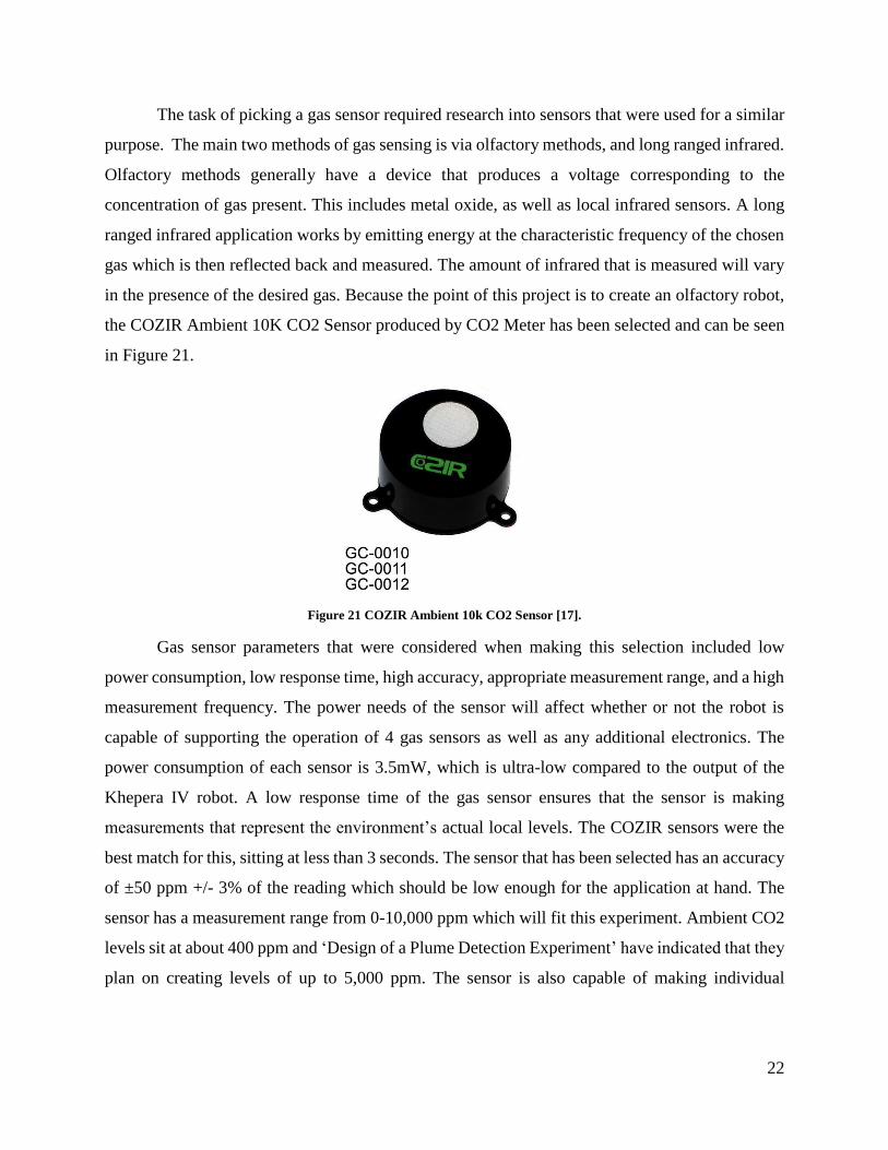
in the presence of the desired gas. Because the point of this project is to create an olfactory robot,
the COZIR Ambient 10K CO2 Sensor produced by CO2 Meter has been selected and can be seen
in Figure 21.
Figure 21 COZIR Ambient 10k CO2 Sensor [17].
Gas sensor parameters that were considered when making this selection included low
power consumption, low response time, high accuracy, appropriate measurement range, and a high
measurement frequency. The power needs of the sensor will affect whether or not the robot is
capable of supporting the operation of 4 gas sensors as well as any additional electronics. The
power consumption of each sensor is 3.5mW, which is ultra-low compared to the output of the
Khepera IV robot. A low response time of the gas sensor ensures that the sensor is making
measurements that represent the environment’s actual local levels. The COZIR sensors were the
best match for this, sitting at less than 3 seconds. The sensor that has been selected has an accuracy
of ±50 ppm +/- 3% of the reading which should be low enough for the application at hand. The
sensor has a measurement range from 0-10,000 ppm which will fit this experiment. Ambient CO2
levels sit at about 400 ppm and ‘Design of a Plume Detection Experiment’ have indicated that they
plan on creating levels of up to 5,000 ppm. The sensor is also capable of making individual
23
measurements every 0.5 seconds. This is one of the highest measurement frequencies for a CO2
sensor so it is well suited for this application.
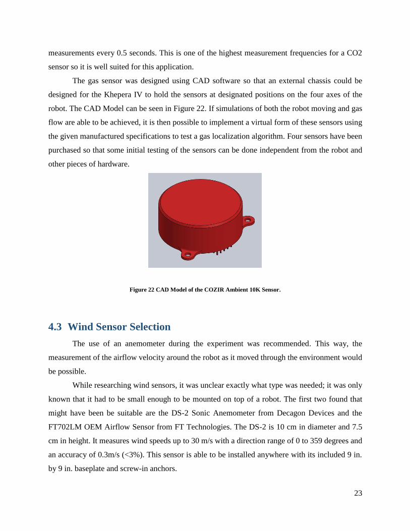
The gas sensor was designed using CAD software so that an external chassis could be
designed for the Khepera IV to hold the sensors at designated positions on the four axes of the
robot. The CAD Model can be seen in Figure 22. If simulations of both the robot moving and gas
flow are able to be achieved, it is then possible to implement a virtual form of these sensors using
the given manufactured specifications to test a gas localization algorithm. Four sensors have been
purchased so that some initial testing of the sensors can be done independent from the robot and
other pieces of hardware.
Figure 22 CAD Model of the COZIR Ambient 10K Sensor.
4.3 Wind Sensor Selection
The use of an anemometer during the experiment was recommended. This way, the
measurement of the airflow velocity around the robot as it moved through the environment would
be possible.
While researching wind sensors, it was unclear exactly what type was needed; it was only
known that it had to be small enough to be mounted on top of a robot. The first two found that
might have been be suitable are the DS-2 Sonic Anemometer from Decagon Devices and the
FT702LM OEM Airflow Sensor from FT Technologies. The DS-2 is 10 cm in diameter and 7.5
cm in height. It measures wind speeds up to 30 m/s with a direction range of 0 to 359 degrees and
an accuracy of 0.3m/s (<3%). This sensor is able to be installed anywhere with its included 9 in.
by 9 in. baseplate and screw-in anchors.
24
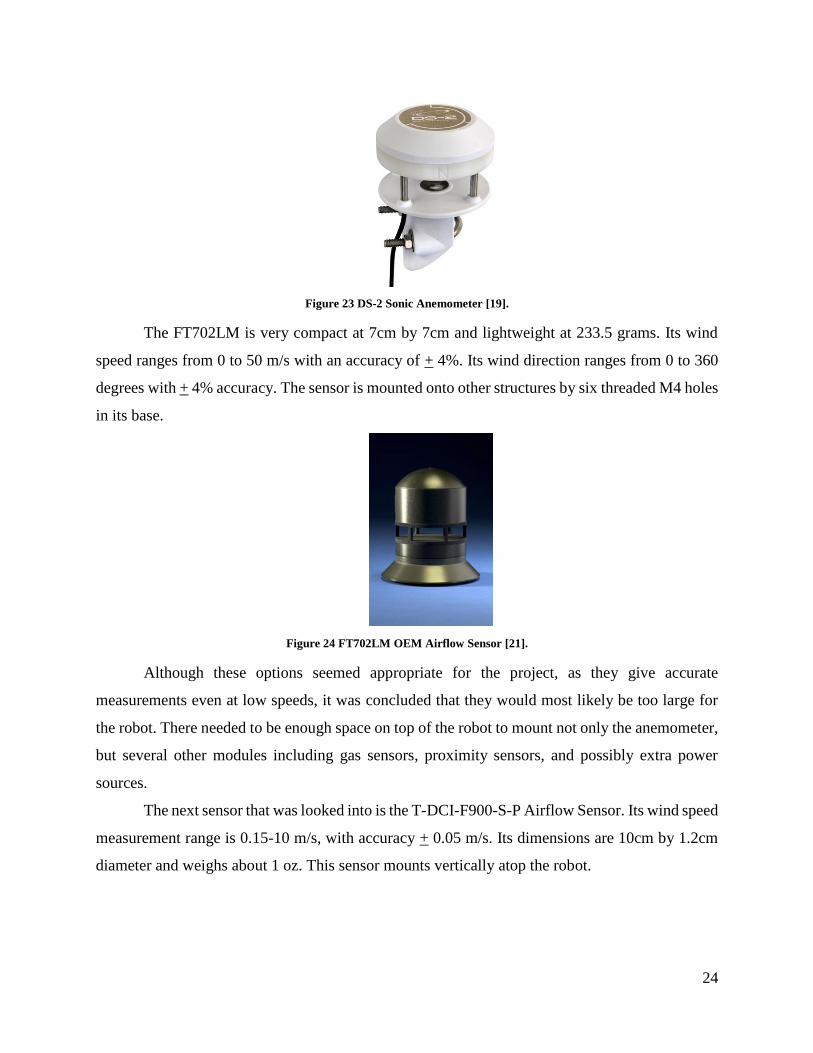
Figure 23 DS-2 Sonic Anemometer [19].
The FT702LM is very compact at 7cm by 7cm and lightweight at 233.5 grams. Its wind
speed ranges from 0 to 50 m/s with an accuracy of + 4%. Its wind direction ranges from 0 to 360
degrees with + 4% accuracy. The sensor is mounted onto other structures by six threaded M4 holes
in its base.
Figure 24 FT702LM OEM Airflow Sensor [21].
Although these options seemed appropriate for the project, as they give accurate
measurements even at low speeds, it was concluded that they would most likely be too large for
the robot. There needed to be enough space on top of the robot to mount not only the anemometer,
but several other modules including gas sensors, proximity sensors, and possibly extra power
sources.
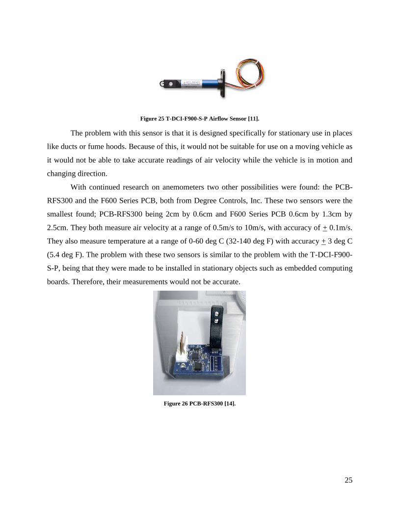
The next sensor that was looked into is the T-DCI-F900-S-P Airflow Sensor. Its wind speed
measurement range is 0.15-10 m/s, with accuracy + 0.05 m/s. Its dimensions are 10cm by 1.2cm
diameter and weighs about 1 oz. This sensor mounts vertically atop the robot.
25
Figure 25 T-DCI-F900-S-P Airflow Sensor [11].
The problem with this sensor is that it is designed specifically for stationary use in places
like ducts or fume hoods. Because of this, it would not be suitable for use on a moving vehicle as
it would not be able to take accurate readings of air velocity while the vehicle is in motion and
changing direction.
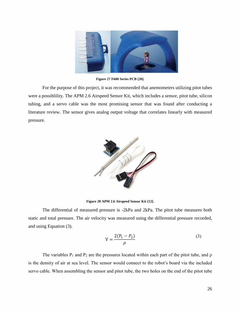
With continued research on anemometers two other possibilities were found: the PCB-
RFS300 and the F600 Series PCB, both from Degree Controls, Inc. These two sensors were the
smallest found; PCB-RFS300 being 2cm by 0.6cm and F600 Series PCB 0.6cm by 1.3cm by
2.5cm. They both measure air velocity at a range of 0.5m/s to 10m/s, with accuracy of + 0.1m/s.
They also measure temperature at a range of 0-60 deg C (32-140 deg F) with accuracy + 3 deg C
(5.4 deg F). The problem with these two sensors is similar to the problem with the T-DCI-F900-
S-P, being that they were made to be installed in stationary objects such as embedded computing
boards. Therefore, their measurements would not be accurate.
Figure 26 PCB-RFS300 [14].
26
Figure 27 F600 Series PCB [20].
For the purpose of this project, it was recommended that anemometers utilizing pitot tubes
were a possiblility. The APM 2.6 Airspeed Sensor Kit, which includes a sensor, pitot tube, silicon
tubing, and a servo cable was the most promising sensor that was found after conducting a
literature review. The sensor gives analog output voltage that correlates linearly with measured
pressure.
Figure 28 APM 2.6 Airspeed Sensor Kit [12].
The differential of measured pressure is -2kPa and 2kPa. The pitot tube measures both
static and total pressure. The air velocity was measured using the differential pressure recorded,
and using Equation (3).
V =
2(P1 − 𝑃2)
𝜌
(3)
The variables P1 and P2 are the pressures located within each part of the pitot tube, and ρ
is the density of air at sea level. The sensor would connect to the robot’s board via the included
servo cable. When assembling the sensor and pitot tube, the two holes on the end of the pitot tube

27
should be placed at least 1cm away from any solid part of the vehicle structure, shown in Fig. 23.
.
Figure 29 APM 2. Airspeed Sensor connected to a board [12].
Figure 30 Pitot tube assembled at nose of UAV [12].
Although this sensor seems like it would be perfect for the mobile terrain robot, a rather
large issue presented itself. Due to error propagation from the micro pressure sensor, this type of
sensor is best when used at higher speeds, such as when placed at the nose of an unmanned air
vehicle (UAV). In order to see how this error will affect measurements at speeds of the Khepera
IV, it was necessary to create an excel spreadsheet to calculate the error in velocity measurements.
This spreadsheet can be seen in Appendix A. For half of the sensor voltages, the pressure
differential is negative, which would not apply to this project at all, due to the nature of Prandtl
tubes and velocity measurements. At maximum ‘actual airspeeds’ of 57.1 m/s, the ‘maximum
error’ in the ‘measured airspeed’ is about 3.89 m/s, which corresponds to about a 6.8% error. At
‘actual airspeeds’ of 0 m/s, the ‘maximum error’ that could occur due to ‘measurement voltage
error’ corresponds to ‘measured airspeeds’ of almost 16 m/s. Because the Khepera IV has a
maximum speed of 1 m/s, this airspeed sensor is by no means practical for this experiment. Despite
28
continuous research on anemometers throughout the duration of the project, a practical airspeed
sensor could not be located.
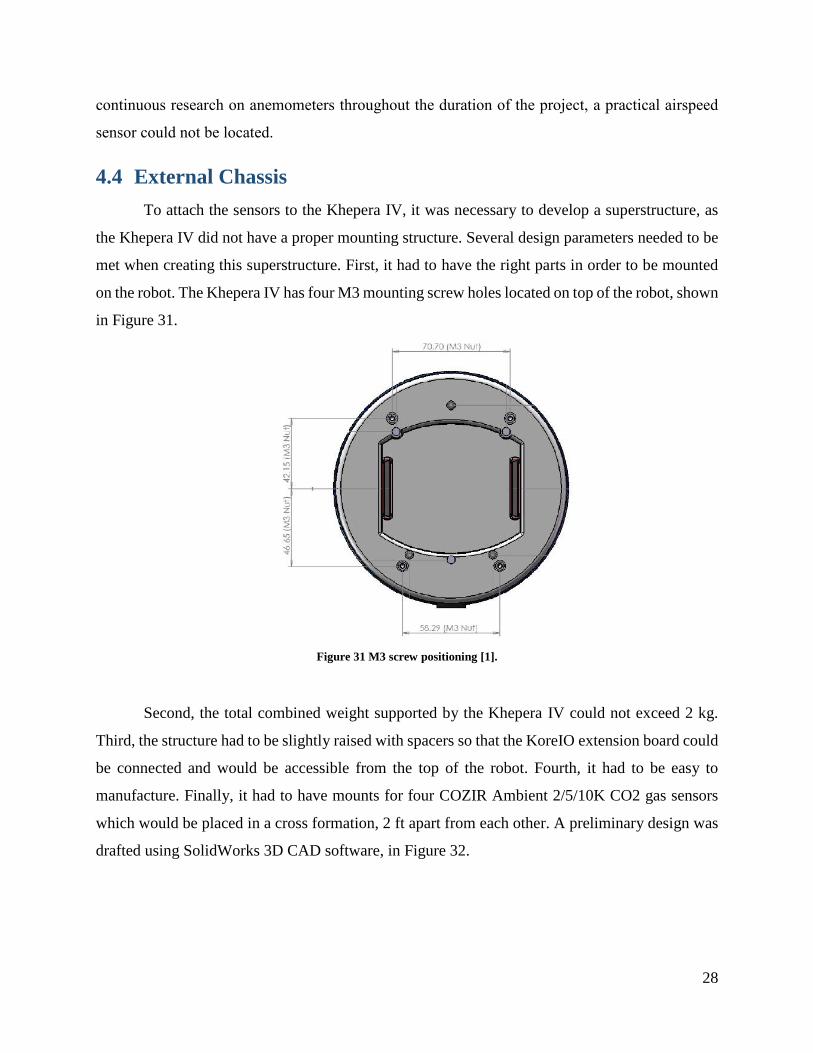
4.4 External Chassis
To attach the sensors to the Khepera IV, it was necessary to develop a superstructure, as
the Khepera IV did not have a proper mounting structure. Several design parameters needed to be
met when creating this superstructure. First, it had to have the right parts in order to be mounted
on the robot. The Khepera IV has four M3 mounting screw holes located on top of the robot, shown
in Figure 31.
Figure 31 M3 screw positioning [1].
Second, the total combined weight supported by the Khepera IV could not exceed 2 kg.
Third, the structure had to be slightly raised with spacers so that the KoreIO extension board could
be connected and would be accessible from the top of the robot. Fourth, it had to be easy to
manufacture. Finally, it had to have mounts for four COZIR Ambient 2/5/10K CO2 gas sensors
which would be placed in a cross formation, 2 ft apart from each other. A preliminary design was
drafted using SolidWorks 3D CAD software, in Figure 32.
29
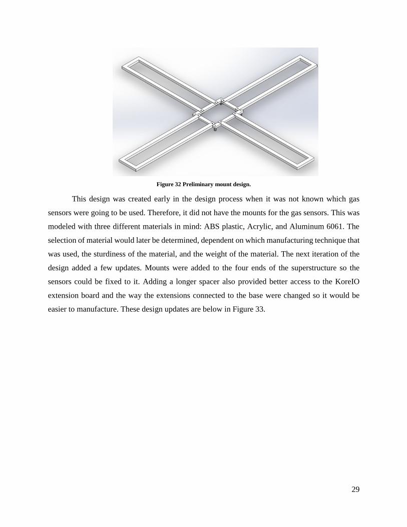
Figure 32 Preliminary mount design.
This design was created early in the design process when it was not known which gas
sensors were going to be used. Therefore, it did not have the mounts for the gas sensors. This was
modeled with three different materials in mind: ABS plastic, Acrylic, and Aluminum 6061. The
selection of material would later be determined, dependent on which manufacturing technique that
was used, the sturdiness of the material, and the weight of the material. The next iteration of the
design added a few updates. Mounts were added to the four ends of the superstructure so the
sensors could be fixed to it. Adding a longer spacer also provided better access to the KoreIO
extension board and the way the extensions connected to the base were changed so it would be
easier to manufacture. These design updates are below in Figure 33.
30
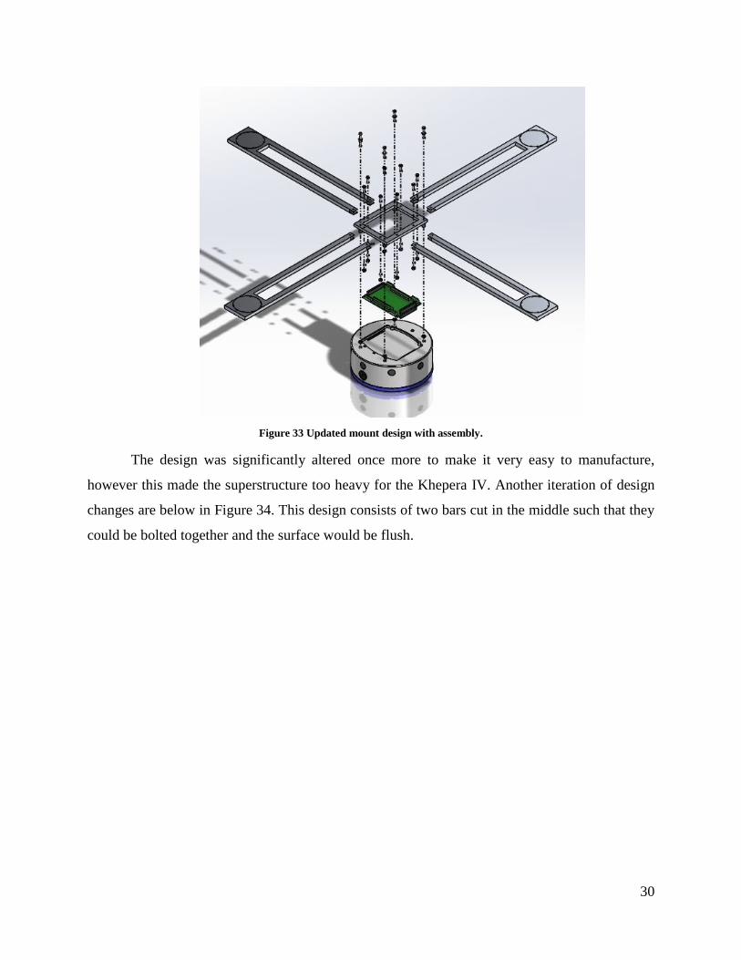
Figure 33 Updated mount design with assembly.
The design was significantly altered once more to make it very easy to manufacture,
however this made the superstructure too heavy for the Khepera IV. Another iteration of design
changes are below in Figure 34. This design consists of two bars cut in the middle such that they
could be bolted together and the surface would be flush.
31
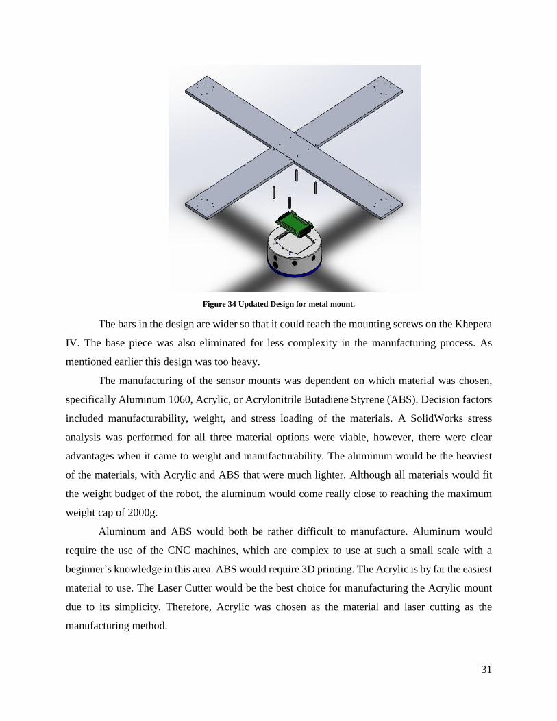
Figure 34 Updated Design for metal mount.
The bars in the design are wider so that it could reach the mounting screws on the Khepera
IV. The base piece was also eliminated for less complexity in the manufacturing process. As
mentioned earlier this design was too heavy.
The manufacturing of the sensor mounts was dependent on which material was chosen,
specifically Aluminum 1060, Acrylic, or Acrylonitrile Butadiene Styrene (ABS). Decision factors
included manufacturability, weight, and stress loading of the materials. A SolidWorks stress
analysis was performed for all three material options were viable, however, there were clear
advantages when it came to weight and manufacturability. The aluminum would be the heaviest
of the materials, with Acrylic and ABS that were much lighter. Although all materials would fit
the weight budget of the robot, the aluminum would come really close to reaching the maximum
weight cap of 2000g.
Aluminum and ABS would both be rather difficult to manufacture. Aluminum would
require the use of the CNC machines, which are complex to use at such a small scale with a
beginner’s knowledge in this area. ABS would require 3D printing. The Acrylic is by far the easiest
material to use. The Laser Cutter would be the best choice for manufacturing the Acrylic mount
due to its simplicity. Therefore, Acrylic was chosen as the material and laser cutting as the
manufacturing method.

32
The WPI Laser Cutter uses a program to convert designs into the machine, which uses an
algorithm and color scheme to make cuts into the desired material. In order to input the 3D parts
into the program, the designs were taken and saved in the desired projected view as drawings
which could be opened up in AutoCAD. After checking the drawings’ dimensions, they are then
able to be used by the machine. The drawings are positioned relative to the rulers on the sides of
the cutting area. After placing the material in the machine at the same place relative to the cuts, a
viewing laser is then used for visual alignment. The program then makes cuts in the parts, leaving
a finished product. The manufactured acrylic mounts are in Figure 35 below.
Figure 35 Updated Sensor Mount Design.
Now that the final design was finished, it was necessary to make sure that it could hold the
sensors properly without significant deformation. To accomplish this, a SolidWorks simulation
add-on was used. A load equal to the weight of the gas sensor was applied on both ends of the
extension pieces. This was done for all three materials on both designs. A more detailed version
of these simulations can be viewed in the Appendix. The conclusion from these studies was that
all three materials would work fine as they did not show any significant deformation.

33
4.5 Price, Weight, and Power Budgets
Over the course of this project, it was important to keep track of a series of budgets for the
robot. This includes a price budget, weight budget, and power budget for the experiment. A price
budget is obviously very important. This ensured that all parts of the experiment could be afforded.
Due to the large expense of the Khepera IV robot, it was necessary to find extra funding in order
to make the purchase and move forward with the project.
A weight budget was important to track due to the design constraints of the robot itself.
The Khepera IV can only carry 2000 grams of external equipment. The biggest concern with
designing the experiment was the weight that an external chassis would add to the project.
Although it would have been desirable to use Aluminum 1060 as the chassis material, it would
have added to much weight to the robot. The use acrylic to manufacture the chassis platform was
chosen to reduce the weight to an amount that the robot could easily handle. The sensors and
required hardware needed to hold together the chassis were also added in the budget.
The third budget looked into was the power budget of the robot. The Khepera IV has a
capability of powering external equipment with 17 Watts at a voltage of 17 V. This would impact
the gas and wind sensors for the experiment. The Khepera IV should easily be able to power these
devices, as the gas sensors have an extremely low power draw, 35 milliWatts per sensor. If not,
then an external battery might need to be purchased.
Figure 36 Budget Chart.
Component Units Voltage (V) Power (mW) Total Power (mW) Weight (g) Total Weight (g) Unit Price Shipping Price Total Price
External Chassis (Acrylic) 2 0 0 0 282.33 564.66 $50.80 $0.00 $101.60
External Chassis (ABS) 2 0 0 0 240.68 481.36 $0.00
External Chassis(Al 1060) 1 0 0 0 629.42 629.42 $0.00
Small Hardware (Screws and Nuts) 1
COZIR Ambient 2/5/10K CO2 Sensor 4 3.3 35 140 20 80 $109.00 $18.48 $454.48
Anemometer 1
KoreIO 1 5 0 0 226.8 226.8 $749.00 $749.00
Khepera IV 1 7.4 -17000 -17000 -2000 -2000 $12,554.00 $12,554.00
Total -16860 -17.76 $13,859.08
Weight BudgetPower Budget Prive Budget

34
4.6 Motion Control/Navigation
4.6.1 Control Modes
The Khepera IV has four different control modes: speed control, speed profile control,
position control, and open loop control. Three of these control modes use a Proportional Integral
Derivative (PID) controller (speed control, speed profile control, and position control). The PID
controller acts on both motors that control each of the wheels. The default PID coefficients are set
at Kp = 10, Ki = 5, Kd = 1 but they can be changed if a particular application requires different
settings. The manual outlines a process to calibrate your PID settings using open loop control [1].
The first control mode is called speed control. In this mode, a speed command is used as
input for each wheel. The allowable speed command ranges from 5 to 1,200. These values
correspond to a wheel speed of 3 mm/s to 813 mm/s. This conversion is done using some geometric
parameters such as the wheel diameter and some intrinsic parameters of the system including the
refresh time and revolution resolution. It simplifies to Equation (4) below [1].
𝑆𝑝𝑒𝑒𝑑 [𝑚𝑚
𝑠] = 0.678181 ∗ 𝑉𝑐𝑜𝑚𝑚𝑎𝑛𝑑
(4)
Speed is the wheel speed in mm/s and Vcommand is the velocity command that is given to the
system. The minimum speed threshold is mostly determined by the PID controller. At low values,
the controller becomes erratic [1]. The maximum threshold is dependent on the battery voltage and
the payload weight. In speed control mode the robot takes the velocity commands and attempts to
reach the velocity as fast as possible. Theoretically the robot would go from zero velocity to the
input instantly. Advantages to this control mode include its simplicity and quick achievement of
the desired speed. The main disadvantage is that with the abrupt speed change it could cause
instability of the payload.
The next control mode is speed profile control. This mode is similar to speed control in
that the system is given two velocity commands, one for each wheel, however in this mode
acceleration ramps are generated so that the change in speed is not as abrupt. The acceleration
ramps are based off of three constants that can be modified. The first constant is Acc_Inc, which
can have a value from 1 – 255 (default: 3). This value is the amount the speed will increase or
decrease for every Acc_Div + 1 control loops. Acc_Div is a value from 0 – 255 (default: 0) that
determines the number of control loops that will pass before Acc_Inc is implemented. The final

35
constant is Min_Speed_Acc which sets the minimum speed so that the speed doesn’t reach a value
that is too low for the PID to handle. Below in Figure 37, is an example of speed profile control
when given three commands, 100 speed units, 200 speed units, and 0 speed units [1].
Figure 37 Speed profile control example [1].
The main advantage of this mode is the increased level of control over the system in order
to keep the robot and its payload stable. The disadvantages include its higher level of complexity
and the long amount of time it takes to obtain the desired speed.
The third control mode is called position control. This mode takes a position command for
each wheel. This command can be anything from 0 – 231 which corresponds to 0 m – 14,563 m. In
a similar conversion process to the speed commands the actual distance can be found using
Equation (5) [1].
𝑃𝑜𝑠𝑖𝑡𝑖𝑜𝑛(𝑚𝑚) =
𝑃𝑐𝑜𝑚𝑚𝑎𝑛𝑑
147.453
(5)
In this equation position is the distance the wheel travels in millimeters and Pcommand is the
given position command. The robot takes the position command and generates a velocity
command as well as an acceleration and a deceleration ramp similar to speed profile control. It
uses the constants that were used in speed profile control as well as three additional constants.
Min_Speed_Dec is like Min_Speed_Acc from speed profile control but it is only used when the

36
robot is decelerating so that it does not reach a low speed that the PID is unable handle (default:
1). Speed_Order determines the maximum speed command that will be allowed (default: 400).
Pos_Margin controls the threshold when the controller stops the motor (ie. Speed = 0). A low value
increases the precision but makes the controller unstable. It is not recommended to go below the
default value of 10 [1]. An example of this control mode can be seen in Figure 38 below. In this
example only one position command is given.
Figure 38 An example of position control [1].
This control mode shares similar advantages and disadvantages as speed profile control but
is tailored to the specific application where the desired distance the robot needs to move is known.
It also increases the complexity and adds more variables.
The final control mode is called open loop control. This mode does not use the PID
controller as the PWM signal is sent directly to the motor. The input commands range from
-2,940 to 2,940, where -2,940 corresponds to full voltage to power the motor backwards and 2,940
corresponds to full voltage to power the motor forwards. There are no acceleration or deceleration
ramps and very little restrictions. Due to the absence of a PID, lower speeds are more stable. In
this mode a higher maximum speed is obtainable but since there is no controller it is more difficult

37
to maintain these speeds. This mode is usually used for crude tests or to tune the PID. It is not
recommended for experimental purposes [1].
4.6.2 Kinematic Motion Study
Calculation of Angular Velocities from X and Y velocities
For this experiment the robot would be receiving the x and y components of velocity from
an algorithm that takes the four gas concentrations from the four sensors and determines the
velocity the robot needs to have to reach a point closer to the source. Since the Khepera IV is a
two wheeled differential drive robot the x and y components of velocity could not be directly used
since the angular velocity of each wheel is all that could be controlled. To make this conversion
some basic calculations were done using Equations (6), (7), (8), and (9) below [18].
𝑽𝒓 = 𝝎𝑹 ∗ 𝒓 (6)
𝑽𝒍 = 𝝎𝒍 ∗ 𝒓 (7)
𝑽𝒊𝒏𝒑𝒖𝒕 = 𝑽𝒓 + 𝑽𝒍
𝟐 (8)
𝝎𝒊𝒏𝒑𝒖𝒕 = 𝑽𝒓 − 𝑽𝒍
𝑳 (9)
In this set of equations Vr is the right wheel velocity, Vl is the left wheel velocity, ωr is the
right wheel angular velocity, ωl is the left wheel angular velocity, r is the radius of the wheel, L is
the distance between the wheels, Vinput is the average velocity of the wheels, and ωinput is the
average angular velocity. Substituting for Vr and Vl into Equation (8) and (9) results in Equations
(10) and (11):
𝑉𝑖𝑛𝑝𝑢𝑡 =
𝑟(𝜔𝑟 + 𝜔𝑙)
2
(10)

38
𝜔𝑖𝑛𝑝𝑢𝑡 =
𝑟(𝜔𝑟 – 𝜔𝑙)
𝐿
(11)
Next these equations were solved for ωr and ωl.
𝜔𝑟 =
2 ∗ 𝑉𝑖𝑛𝑝𝑢𝑡 + 𝜔𝑖𝑛𝑝𝑢𝑡 ∗ 𝐿
2 ∗ 𝑟
(12)
𝜔𝑙 = 2 ∗ 𝑉𝑖𝑛𝑝𝑢𝑡 − 𝜔𝑖𝑛𝑝𝑢𝑡 ∗ 𝐿
2 ∗ 𝑟 (13)
In this system Vinput is the same as the desired velocity. This is given by the following:
𝑉𝑖𝑛𝑝𝑢𝑡 = 𝑉𝑑𝑒𝑠𝑖𝑟𝑒𝑑 = √𝑉𝑥
2 + 𝑉𝑦2
(14)
ωinput is a comparison with the desired angular velocity and the difference between the actual angle
and the desired angle. This is determined by Equation (15) below.
𝜔𝑖𝑛𝑝𝑢𝑡 = 𝑑𝑒𝑠𝑖𝑟𝑒𝑑 − 𝑎(𝜃𝑎𝑐𝑡𝑢𝑎𝑙 − 𝜃𝑑𝑒𝑠𝑖𝑟𝑒𝑑) (15)
θdesired and 𝑑𝑒𝑠𝑖𝑟𝑒𝑑 are defined in Equation (16) and (17) below.
𝜃𝑑𝑒𝑠𝑖𝑟𝑒𝑑 = tan−1(
𝑉𝑦
𝑉𝑥)
(16)
𝑑𝑒𝑠𝑖𝑟𝑒𝑑 = 𝑑𝜃
𝑑𝑡 (17)
In this instance, a is a constant gain which alters the dependence of 𝜔𝑖𝑛𝑝𝑢𝑡 on the measured value
as opposed to the desired value and 𝜃𝑎𝑐𝑡𝑢𝑎𝑙 is the previous measurement of the pose. Finally the
angular velocities of the wheels (the inputs to the robot) have been determined in terms of the x
and y components of the velocity (the inputs to the system) and known constants. These are
pictured in Equation (18) and (19).

39
𝜔𝑟 = 2 ∗ √𝑉𝑥
2 + 𝑉𝑦2 + (
𝑑 tan−1 (𝑉𝑦
𝑉𝑥)
𝑑𝑡− 𝑎 (𝜃𝑎𝑐𝑡𝑢𝑎𝑙 − tan−1 (
𝑉𝑦
𝑉𝑥))) ∗ 𝐿
2 ∗ 𝑟
(18)
𝜔𝑙 = 2 ∗ √𝑉𝑥
2 + 𝑉𝑦2 − (
𝑑 tan−1 (𝑉𝑦
𝑉𝑥)
𝑑𝑡− 𝑎 (𝜃𝑎𝑐𝑡𝑢𝑎𝑙 − tan−1 (
𝑉𝑦
𝑉𝑥))) ∗ 𝐿
2 ∗ 𝑟
(19)
To turn these into linear velocities, both sides need to be multiplied by the radius, resulting in
Equation (20) and (21).
𝑉𝑟 = 2 ∗ √𝑉𝑥
2 + 𝑉𝑦2 + (
𝑑 tan−1 (𝑉𝑦
𝑉𝑥)
𝑑𝑡− 𝑎 (𝜃𝑎𝑐𝑡𝑢𝑎𝑙 − tan−1 (
𝑉𝑦
𝑉𝑥))) ∗ 𝐿
2
(20)
𝑉𝑙 = 2 ∗ √𝑉𝑥
2 + 𝑉𝑦2 − (
𝑑 tan−1 (𝑉𝑦
𝑉𝑥)
𝑑𝑡− 𝑎 (𝜃𝑎𝑐𝑡𝑢𝑎𝑙 − tan−1 (
𝑉𝑦
𝑉𝑥))) ∗ 𝐿
2
(21)
Simulink model
Another step to this project was to simulate the robot’s motion and the controller using
software. To do this a Simulink model was set up to generate an artificial path for the robot based
off of a known set of parametric equations. It utilizes the desired x and y velocities, which are time
dependent, to generate the robot’s simulated motion. The Simulink model consisted of four blocks.

40
The main model can be viewed below in Figure 39. The different subsystems can be viewed in
appendix D.
Figure 39 Main Simulink model.
In this model, there are four subsystems. The first subsystem on the left generates the
artificial path. It sets up equations based off of the parametric equations for the x and y velocities
as well as their positions. In the real experiment, the x and y desired positions would not be known,
only the velocities. For the sake of this model, however, comparing the actual x and y positions
that are received at the end of the simulation with the desired positions is beneficial because it
shows how well the controller works. As shown in the figure, the desired x and y positions go
straight to a graphing block, which plots them against each other. The parametric model of a
bifolium was used for the first simulation. These equations can be seen in Equation (22), (23),
(24), and (25).
𝑉𝑥 = 2 ∗ 𝑏 ∗ sin (4 ∗ 𝑡) (22)
𝑉𝑦 = 4 ∗ 𝑏 ∗ sin2(𝑡) ∗ (2 ∗ cos(2 ∗ 𝑡) + 1) (23)
𝑥 = 4 ∗ 𝑏 ∗ sin2(𝑡) ∗ 𝑐𝑜𝑠2(𝑡) (24)
𝑦 = 4 ∗ 𝑏 ∗ 𝑠𝑖𝑛3(𝑡) ∗ cos (𝑡) (25)
41
The next subsystem in the model is the controller. This subsystem takes the x and y desired
velocities and turns them into Vinput and ωinput using equations (14) and (15) above. The next
subsystem block creates the angular velocities, which will be the actual input into the robot. This
is done using equations (18) and (19) above. These angular velocities are also used later when a
3D simulation of the model was created.
The final subsystem block takes Vinput and ωinput and applies them to the kinematic
equations for the Khepera IV. Equations (26), (27), and (28) show these relationships.
𝑎𝑐𝑡𝑢𝑎𝑙 = 𝑉𝑖𝑛𝑝𝑢𝑡 ∗ cos(𝜃𝑎𝑐𝑡𝑢𝑎𝑙) (26)
𝑎𝑐𝑡𝑢𝑎𝑙 = 𝑉𝑖𝑛𝑝𝑢𝑡 ∗ sin( 𝜃𝑎𝑐𝑡𝑢𝑎𝑙) (27)
𝑎𝑐𝑡𝑢𝑎𝑙 = 𝜔𝑖𝑛𝑝𝑢𝑡 (28)
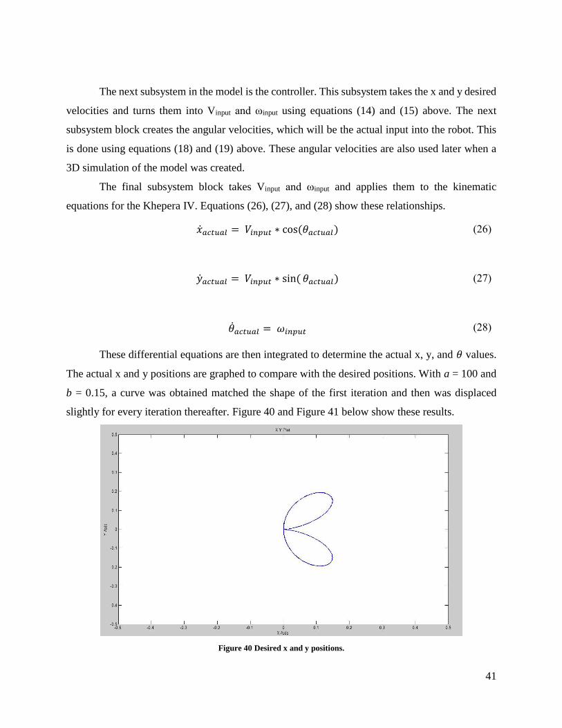
These differential equations are then integrated to determine the actual x, y, and 𝜃 values.
The actual x and y positions are graphed to compare with the desired positions. With a = 100 and
b = 0.15, a curve was obtained matched the shape of the first iteration and then was displaced
slightly for every iteration thereafter. Figure 40 and Figure 41 below show these results.
Figure 40 Desired x and y positions.

42
Figure 41 Actual x and y positions.
The time interval for this simulation was very short at only ten seconds. This resulted in
very high angular velocities for the wheels which were above the maximum speed for the khepera
(.88 m/s). To remedy this situation the parametric equations had to be modified by dividing t by a
constant. Changing the x and y positions in this fashion also changes their derivatives, the x and y
velocities, so they had to be found again. Another alteration made for the next iteration of
simulations was the constant b. This value was changed from .15 to 2.5 to increase the area of the
simulation to approximately 5 by 5 meters which is closer to the area an actual experiment would
be held in. Making these changes garnered more realistic results within the Khepera’s speed ranges
and also allowed the gain (a) to be lowered significantly and still obtain close results.
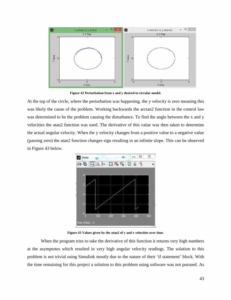
There was still one problem with the model however; at one point in the simulation there
would be a sharp spike in the angular velocities of the wheels causing a perterbation in the x and
y position that was well off the desired track. Thinking this problem might be due to the complexity
of the bifolium shape, the code was altered to follow a cricular path instead. The block for this
subsystem can be seen in appendix D. Running simulations with this shape allowed the problem
to become more apparent. In Figure 42 below is the perterbation in the shape at the very top of the
circle.
43
Figure 42 Perturbation from x and y desired in circular model.
At the top of the circle, where the perturbation was happening, the y velocity is zero meaning this
was likely the cause of the problem. Working backwards the arctan2 function in the control law
was determined to be the problem causing the disturbance. To find the angle between the x and y
velocities the atan2 function was used. The derivative of this value was then taken to determine
the actual angular velocity. When the y velocity changes from a positive value to a negative value
(passing zero) the atan2 function changes sign resulting in an infinite slope. This can be observed
in Figure 43 below.
Figure 43 Values given by the atan2 of y and x velocities over time.
When the program tries to take the derivative of this function it returns very high numbers
at the asymptotes which resulted in very high angular velocity readings. The solution to this
problem is not trivial using Simulink mostly due to the nature of their ‘if statement’ block. With
the time remaining for this project a solution to this problem using software was not pursued. As

44
a result when controlling the robot using this code one should not go to very low velocities. The
Khepera PID controller does not allow the robot to go to low velocities, as outlined in previous
sections, likely due to a similar issue [1]. Since the problem was known the parametric equations
were changed one more time to generate a shape that didn’t require a low y velocity; half of a
parabola. Finally, the simulation ran smoothly and generated the expected result. The results for a
90 second simulation can be seen in Figure 44 below.
Figure 44 Final simulation run for the half parabola shape.
4.6.3 Simulations
Preliminary Simulation
Using the K-team sponsored V-rep simulation software, a very basic preliminary
simulation of the experiment was created. Since the Khepera IV is K-team’s brand new model, it
was not available in the software so the Khepera III was used. The basic goal of this simulation
was to be able to view, in three dimensions, the robot reacting correctly to simulated gas sensor
input, and to be able to use the infrared sensors to avoid running into walls.
Since the program could not simulate gas concentrations and experiments were not actually
run to obtain actual plume concentration data, random numbers were generated to act as input from
each sensor. Since there were four sensors, four random numbers were generated. These numbers
ranged from 400 to 2500, except for the rear sensor which ranged from 400 to 600. The range for
the rear sensor was much smaller because when the robot is moving towards a gas source, the
concentration reading of the gas behind the robot should always be smaller than the concentration

45
readings from the other sensors. For every loop of the program, a new number was generated for
each sensor. The robot would act accordingly, depending on which sensor had the highest reading.
For example if the front sensor reading was the highest, then both wheels were given the maximum
velocity command, resulting in forward motion. If the right sensor was the highest, then the left
wheel would be given the maximum velocity command and the right wheel would be given the
negative maximum velocity command, resulting in a turn-in-place to the right. The opposite is true
if the left sensor was the highest reading. If the rear sensor was the highest then both wheels would
be given the negative velocity command resulting in backwards motion.
The final part to the simulation was the wall avoidance. The simulated experimental setup
was a 5m by 5m box surrounded by walls. Using the front five infrared sensors, the robot can
determine how far away it is from a wall. If the value of any of these sensors dropped too low then
the robot would turn away from the wall. In this program the robot uses the speed control mode
which is outlined in the previous section. This is the only mode that can be used in this software.
The source code for this simulation can be viewed in the appendix and the actual simulations can
be viewed online [8] [9].
Simulation with Angular Velocity Data
To test the accuracy of the Simulink program a simulation was run using the angular
velocities that were generated by it. Since V-rep did not have the Khepera IV, the Khepera III’s
constants for the radius of the wheels and distance between the wheels were used in the code.
Another issue with using V-rep for simulation purposes was that the maximum velocity of the
Khepera III in V-rep was only 0.129 m/s, which is nowhere near the actual maximum velocity of
the Khepera IV (0.88 m/s) [1]. Therefore, the maximum speed of the robot in the Simulink
simulation could not exceed this value. With all of this taken into account, a program was written
that would change each wheel’s angular velocity at each time interval based on the simulation data
received from the Simulink program. This program can be seen in Appendix E. The simulation ran
properly and performed as expected. The video of this simulation can be viewed online [10]. Below
in Figure 45 is an image showing the final shape of the path the robot took using the data from the
half parabola simulation.

46
Figure 45 Final shape generated by the V-rep software using the data for the half parabola simulation.
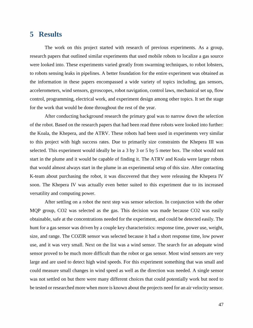
47
5 Results
The work on this project started with research of previous experiments. As a group,
research papers that outlined similar experiments that used mobile robots to localize a gas source
were looked into. These experiments varied greatly from swarming techniques, to robot lobsters,
to robots sensing leaks in pipelines. A better foundation for the entire experiment was obtained as
the information in these papers encompassed a wide variety of topics including, gas sensors,
accelerometers, wind sensors, gyroscopes, robot navigation, control laws, mechanical set up, flow
control, programming, electrical work, and experiment design among other topics. It set the stage
for the work that would be done throughout the rest of the year.
After conducting background research the primary goal was to narrow down the selection
of the robot. Based on the research papers that had been read three robots were looked into further:
the Koala, the Khepera, and the ATRV. These robots had been used in experiments very similar
to this project with high success rates. Due to primarily size constraints the Khepera III was
selected. This experiment would ideally be in a 3 by 3 or 5 by 5 meter box. The robot would not
start in the plume and it would be capable of finding it. The ATRV and Koala were larger robots
that would almost always start in the plume in an experimental setup of this size. After contacting
K-team about purchasing the robot, it was discovered that they were releasing the Khepera IV
soon. The Khepera IV was actually even better suited to this experiment due to its increased
versatility and computing power.
After settling on a robot the next step was sensor selection. In conjunction with the other
MQP group, CO2 was selected as the gas. This decision was made because CO2 was easily
obtainable, safe at the concentrations needed for the experiment, and could be detected easily. The
hunt for a gas sensor was driven by a couple key characteristics: response time, power use, weight,
size, and range. The COZIR sensor was selected because it had a short response time, low power
use, and it was very small. Next on the list was a wind sensor. The search for an adequate wind
sensor proved to be much more difficult than the robot or gas sensor. Most wind sensors are very
large and are used to detect high wind speeds. For this experiment something that was small and
could measure small changes in wind speed as well as the direction was needed. A single sensor
was not settled on but there were many different choices that could potentially work but need to
be tested or researched more when more is known about the projects need for an air velocity sensor.
48
With both the robot and the sensor selection out of the way the sensor mount was focused
on. The top of the robot is very small but has four screw holes for M3 screws in it. It was decided
that these holes would be used to attach the mount for the sensors. The mount was designed using
SolidWorks CAD software and a couple design constraints. There was a need for four gas sensors
placed in a cross formation separated by at least two feet. The mount also needed to be raised
slightly because the KoreIO board used for connecting the sensors would be underneath the mount.
The total payload weight could also not exceed 2000 grams. The design went through much
iteration to make it sturdier, lighter, and more manufacturable. The final design was very simple
and used acrylic for a material. It was made on campus using the WPI machine lab’s laser cutter.
To make sure the design choices were within the constraints of the hardware and funding,
a price, weight, and power budget were made. The sensor mount was lightweight as it was made
out of acrylic. The sensors were very small and also didn’t draw very much power. The restrictions
of the weight and power budget were met with, leaving room to spare for extra sensors, or add-ons
if it is later determined to be necessary. The price budget was a little high but was within the limits
given.
Since the robot was never obtained running motion simulations was the next best thing. A
kinematic control law was derived and used for this purpose. It was built into a Simulink model
that took a desired x and y velocity and converted into the Khepera’s actual motion. This model
had multiple hiccups and required fine tuning but a working model was achieved. The final step
for the simulation was to take the data the Simulink model generated for the angular velocities of
the Khepera’s wheels and apply this to the V-rep model of the Khepera to see if the motions
matched. A successful simulation was created in V-rep using this method.

49
6 Conclusions and Recommendations
6.1 Conclusions
Although all of the goals were not completed, as this group was the first to take on this
project, several sub goals were completed to set up the success of future groups that will continue
this work. The Khepera IV was selected for this experiment and the quotes were obtained for its
purchase. A gas as well as gas sensors were also selected. The gas sensors were purchased and are
available for use for future projects. A mounting system for the sensors that is flexible and can be
modified for different sensor configurations was designed and manufactured. The kinematic
motion equations for the Khepera IV were derived and used to accurately model its motion.
An outstanding wind sensor was not found. Some choices that could be used in future
projects were discussed, but they would require further testing or research.
It was determined that there is no need for a separate wireless communication system as
the Khepera IV is capable of both radio and Bluetooth communication. The sensors connect to the
KoreIO extension board which connects to the Khepera IV so the robot should be able to transmit
the sensor data to a base station and receive further commands. This was not tested as there was
no access to the actual robot.
The data acquisition system was worked on sparingly, but it was not tested in an
experimental environment. Data was tracked and logged using the software that came with the
CO2 sensors. A LabVIEW program was also provided by the company that provided the sensors.
The data logging works independent of the robot, but might need some modification when actually
working with the robot.
The robot was never acquired while conducting the MQP and therefore the actual
experiment was not run. This means a program that controlled the robots motion was not
implemented, a gas source was not localized, and a gas plume was not reconstructed. Although
the main goals which required experiments were not met, the leg work was provided that will
lead to the success of future experiments. The next group that works on this project will have a
robot, the sensors, a mounting system, and a working simulation software to play with. They will
be able to jump right in to the experiment and work on the aspects that were not possible for this
project.

50
6.2 Recommendations
The majority of this report is a recommendation for a future experiment. The Khepera IV
robot made by K-team and CO2 is recommended for the robot and for the gas used in the
experiment for reasons outlined in this paper. The COZIR gas sensors and a mount design similar
to the one that was designed for this project is recommended for the continuation of this project.
The mount design and CAD models can be modified very easily using the laser cutter in Washburn
Shops at WPI. If any sensors or hardware are added later the design can be modified to fit these
needs.
The wind sensor selection should be researched further. The exact purpose of reading air
velocity should be determined and then finding the correct wind sensor should be clearer. During
this project, the physical experiment was never conducted so it was not known whether or not there
was going to be a fan adding air flow to the experiment. During this project it was also unclear
whether or not the direction of the air flow was important, which is something very few micro
wind sensors can provide. If it is later determined that an air velocity sensor is needed to improve
the algorithm that runs the robot, then the ones listed in this report should be researched more
thoroughly. One should then be selected based on the data that is needed for the algorithm.
During the research portion of a future MQP, various programming languages should be
studied. The simulation software for this project was written in Simulink and Matlab, The robot
simulation software, V-rep, uses a language called LUA to drive its simulations. The makers of
this software claim that it can use seven different programming approaches and any programming
language using remote API, add-ons, and plug-ins. These features were attempted, but did not
work successfully due to unfamiliarity with the software and these techniques. Learning C or C++
is highly recommended, as this is what the Khepera IV robot is coded in. Familiarity with the
Linux operating system will also be useful because the robot is controlled by a microcontroller
with a Linux operating system and requires a computer with Linux to communicate with it.
Finally, it is recommended that future project groups start working on the experiment
portion of the project as soon as possible. Working on a new robot that will constantly be
communicating with a base station, sending back and forth sensor data and motion commands, is
a complex system that will take many trials and debugging sessions to work properly. The more
time that is spent experimenting with the setup and trying new things, the more likely the
experiment will be successful. Also, if there are two groups working together, similar to this

51
project, make sure the communication between groups is sufficient. Work is often difficult to
accomplish when there are two groups working on different things and they are not on the same
page.
52
References
[1] Carron, T., Lambercy, F., and Tharin, J., 2014, Khepera IV User Manual, K-team, Vallorbe,
Switzerland
[2] Clark, C., Greene, M., and Seigle, M., 2015, “Design of Plume Generation and Detection
Systems,” NAG-1501, Worcester Polytechnic Institute, Worcester, MA.
[3] Demetriou, M. A., Gatsonis, N.A., and Court, J., “A coupled controls-computational fluids
approach for the estimation of the concentration from a moving gaseous source in a 2D
domain with a Lyapunov-guided sensing aerial vehicle”, IEEE Transactions on Control
Systems Technology, Vol. 22, 3, pp. 853 – 867, 2014. 10.1109/TCST.2013.2267623
[4] Duckett, T., Lilienthal, A., Wandel, M., Weimar, U., and Zell, A., 2014, “Gas Distribution in
Unventilated Indoor Environments Inspected by a Mobile Robot,” IEEE International
Conference on Advanced Robotics, Coimbra, Portugal
[5] Faria, R., Marques, L., Marjovi, A., Nunes, J., and Sousa, P., 2010, “An Olfactory-Based
Robot Swarm Navigation Method,” IEEE International Conference on Robotics and
Automation, Coimbra Portugal
[6] Hugues, E., Martinez, D., and Rochel O., 2006, “A Biomimetic Robot for Tracking Specific
Odors in Turbulent Plumes,” Springer Science, LLC Auton Robot, Vandoeuvre-Les-
Nancy, France
[7] Lambercy, F., and Tharin, J., 2013, Khepera III User Manual, K-team, Vallorbe, Switzerland
[8] Myles, M.. (2014, December 4). Khepera III simulation 1 [Video file]. Retrieved from
https://www.youtube.com/watch?v=Qyek_jrcHkk&feature=youtu.be
[9] Myles, M.. (2014, December 4). Khepera III simulation 2 [Video file]. Retrieved from
https://www.youtube.com/watch?v=yoM3ofunZvg&feature=youtu.be
[10] Myles, M.. (2015, February 27). Final Khepera Control Simulation Parabola [Video file].
Retrieved from https://www.youtube.com/watch?v=yoM3ofunZvg&feature=youtu.be
[11] “Air Velocity Sensor - T-DCI-F900-S-P.” Onset Computer Corporation: Onset HOBO Data
Loggers. N.p., n.d. Web. 04 Mar. 2015. < http://www.onsetcomp.com/products/sensors/t-
dci-f900-s-p>.
[12] “APM 2.6 Airspeed Sensor Kit.” 3D Robotics Inc. N.p., n.d. Web. 04 Mar. 2015. <
https://store.3drobotics.com/products/>.
[13] “ATRV-Jr Mobile Robot Tech Sheet.” Real World Interface. N.p., n.d. Web. 04 Mar. 2015.
<http://www.ing.unibs.it/>.
[14] “Board-Mounted Air Velocity & Temperature Sensor with Reference Circuit • PCB-
RFS300.” Degree Controls, Inc. N.p., n.d. Web. 04 Mar. 2015. <
http://www.degreec.com/downloads/airflow-sensors/rfs300.pdf>.
[15] “Clifford Rover.” NASA Jet Propulsion Laboratory. N.p., n.d. Web. 04 Mar. 2015.
<https://www-robotics.jpl.nasa.gov/>.
53
[16] "Coppelia Robotics V-rep: Create. Compose. Simulate. Any Robot." Coppelia Robotics V-
rep: Create. Compose. Simulate. Any Robot. N.p., n.d. Web. 03 Mar. 2015.
<http://www.coppeliarobotics.com/>.
[17] “COZIR Ambient 2/5/10K CO2 Sensor.” CO2meter.com: CO2 Measurement Specialists.
N.p., n.d. Web. 04 Mar. 2015. < http://www.co2meter.com/>.
[18] "Differential Drive Robotics." 1 Differential Drive Kinematics (n.d.): n. pag. Berkeley.edu.
Web. 03 Mar. 2015.
<http://chess.eecs.berkeley.edu/eecs149/documentation/differentialDrive.pdf>.
[19] “DS-2 Sonic Anemometer.” Decagon Devices. N.p., n.d. Web. 04 Mar. 2015.
<http://www.decagon.com/products/>.
[20] “F600 Series PCB Embedded Air Velocity and Temperature Sensor Data Sheet.” Degree
Controls, Inc. N.p., n.d. Web. 04 Mar. 2015. <
http://www.degreec.com/downloads/airflow-sensors/f600/f600-datasheet.pdf>.
[21] “FT702LM wind sensor.” FT Technologies LTD. N.p., n.d. Web. 04 Mar. 2015. <
http://www.fttech.co.uk/ft702-lm-wind-sensor/>.
[22] “K-Team Corporation | Mobile Robotics.” K-Team Corporation. N.p., n.d. Web. 03 Mar.
2015.[23] “Simplify Hybrid Electric Vehicle Modelingwith Simscape.” MathWorks.
N.p., n.d. Web. 03 Mar. 2015. <http://www.mathworks.com/>.
[24] “The Programming Language Lua.” The Programming Language Lua. N.p., n.d. Web. 03
Mar. 2015. <http://www.lua.org/>.[25] “University of Tubingen: Outdoor Robot.”
University of Tubingen. N.p., n.d. Web. 04 Mar. 2015. < http://www.ra.cs.uni-
tuebingen.de/>.
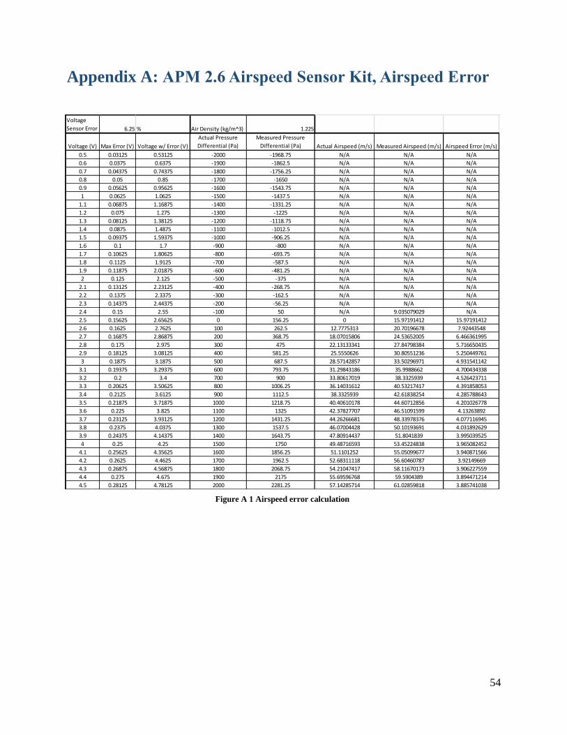
54
Appendix A: APM 2.6 Airspeed Sensor Kit, Airspeed Error
Voltage
Sensor Error 6.25 % Air Density (kg/m^3) 1.225
Voltage (V) Max Error (V) Voltage w/ Error (V)
Actual Pressure
Differential (Pa)
Measured Pressure
Differential (Pa) Actual Airspeed (m/s) Measured Airspeed (m/s) Airspeed Error (m/s)
0.5 0.03125 0.53125 -2000 -1968.75 N/A N/A N/A
0.6 0.0375 0.6375 -1900 -1862.5 N/A N/A N/A
0.7 0.04375 0.74375 -1800 -1756.25 N/A N/A N/A
0.8 0.05 0.85 -1700 -1650 N/A N/A N/A
0.9 0.05625 0.95625 -1600 -1543.75 N/A N/A N/A
1 0.0625 1.0625 -1500 -1437.5 N/A N/A N/A
1.1 0.06875 1.16875 -1400 -1331.25 N/A N/A N/A
1.2 0.075 1.275 -1300 -1225 N/A N/A N/A
1.3 0.08125 1.38125 -1200 -1118.75 N/A N/A N/A
1.4 0.0875 1.4875 -1100 -1012.5 N/A N/A N/A
1.5 0.09375 1.59375 -1000 -906.25 N/A N/A N/A
1.6 0.1 1.7 -900 -800 N/A N/A N/A
1.7 0.10625 1.80625 -800 -693.75 N/A N/A N/A
1.8 0.1125 1.9125 -700 -587.5 N/A N/A N/A
1.9 0.11875 2.01875 -600 -481.25 N/A N/A N/A
2 0.125 2.125 -500 -375 N/A N/A N/A
2.1 0.13125 2.23125 -400 -268.75 N/A N/A N/A
2.2 0.1375 2.3375 -300 -162.5 N/A N/A N/A
2.3 0.14375 2.44375 -200 -56.25 N/A N/A N/A
2.4 0.15 2.55 -100 50 N/A 9.035079029 N/A
2.5 0.15625 2.65625 0 156.25 0 15.97191412 15.97191412
2.6 0.1625 2.7625 100 262.5 12.7775313 20.70196678 7.92443548
2.7 0.16875 2.86875 200 368.75 18.07015806 24.53652005 6.466361995
2.8 0.175 2.975 300 475 22.13133341 27.84798384 5.716650435
2.9 0.18125 3.08125 400 581.25 25.5550626 30.80551236 5.250449761
3 0.1875 3.1875 500 687.5 28.57142857 33.50296971 4.931541142
3.1 0.19375 3.29375 600 793.75 31.29843186 35.9988662 4.700434338
3.2 0.2 3.4 700 900 33.80617019 38.3325939 4.526423711
3.3 0.20625 3.50625 800 1006.25 36.14031612 40.53217417 4.391858053
3.4 0.2125 3.6125 900 1112.5 38.3325939 42.61838254 4.285788643
3.5 0.21875 3.71875 1000 1218.75 40.40610178 44.60712856 4.201026778
3.6 0.225 3.825 1100 1325 42.37827707 46.51091599 4.13263892
3.7 0.23125 3.93125 1200 1431.25 44.26266681 48.33978376 4.077116945
3.8 0.2375 4.0375 1300 1537.5 46.07004428 50.10193691 4.031892629
3.9 0.24375 4.14375 1400 1643.75 47.80914437 51.8041839 3.995039525
4 0.25 4.25 1500 1750 49.48716593 53.45224838 3.965082452
4.1 0.25625 4.35625 1600 1856.25 51.1101252 55.05099677 3.940871566
4.2 0.2625 4.4625 1700 1962.5 52.68311118 56.60460787 3.92149669
4.3 0.26875 4.56875 1800 2068.75 54.21047417 58.11670173 3.906227559
4.4 0.275 4.675 1900 2175 55.69596768 59.5904389 3.894471214
4.5 0.28125 4.78125 2000 2281.25 57.14285714 61.02859818 3.885741038
Figure A 1 Airspeed error calculation
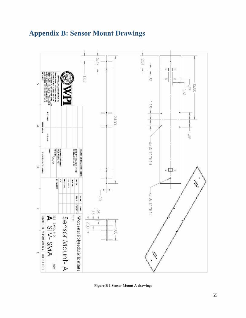
55
Appendix B: Sensor Mount Drawings
Figure B 1 Sensor Mount A drawings

56
Figure B 2 Sensor mount B drawings
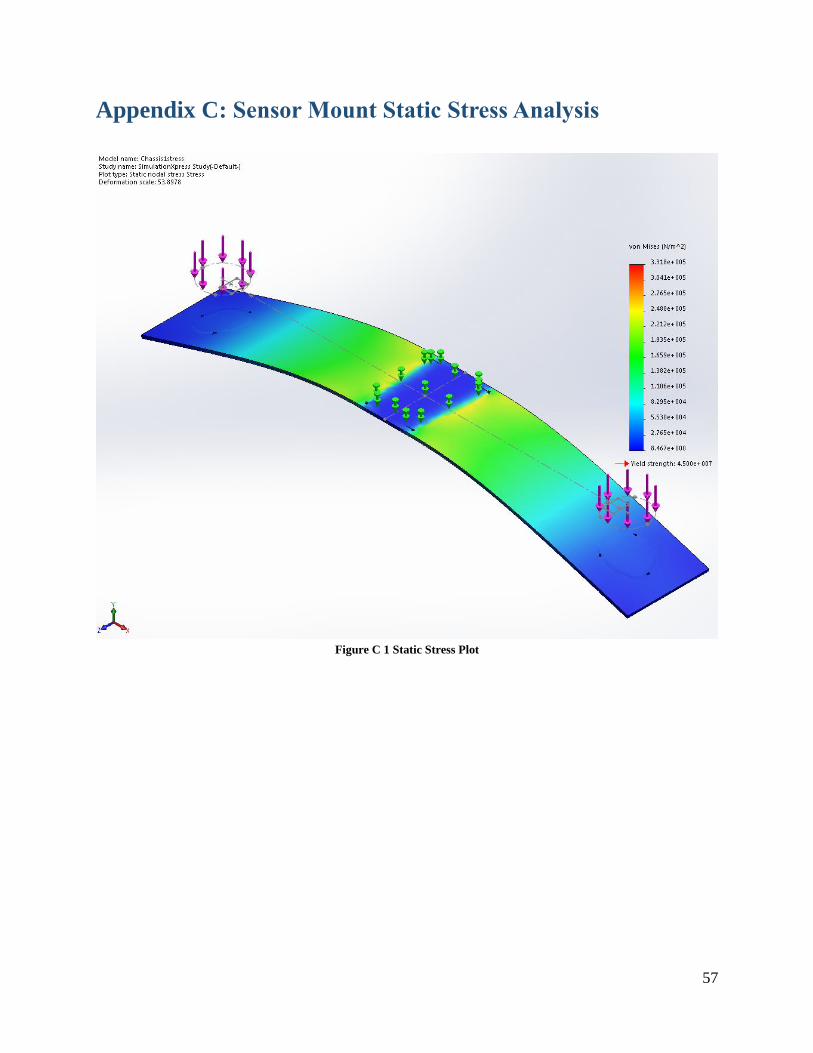
57
Appendix C: Sensor Mount Static Stress Analysis
Figure C 1 Static Stress Plot

58
Figure C 2 Static Displacement Plot

59
Figure C 3 Factor of Safety Check
60
Appendix D: Simulink Robot Control Code
a = 2.5; d = .0884; r = .0205;
Matlab script that sets the constants for the Simulink program. a = constant that scales the
parametric shape. d = distance between the wheels of the robot in meters. r = radius of the
wheels in meters.
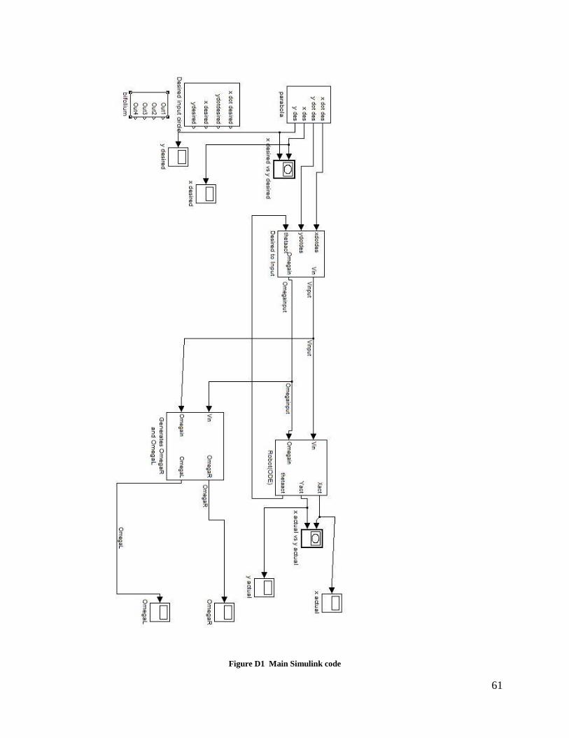
61
Figure D1 Main Simulink code

62
Figure D2 Parametric equations for a bifolium in Simulink

63
Figure D3 Parametric equations for a circle in Simulink
Figure D4 Parametric equations for a parabola in Simulink

64
Figure D5 Controller used in Simulink model. Takes in Xdotdesired and Ydotdesired, returns Vin and OmegaIn
Figure D6 Simulink block that converts Vin and Omegain to angular velocities of both wheels

65
Figure D7 Simulink block that converts Vin and Omegain to angular velocities of both wheels

66
Appendix E : V-rep Simulation Code
LUA code used for first simulation with random sensor generation and infrared wall detection:
-- This script runs in a thread. A non-threaded script can also be used instead
-- Following commands are implemented:
--
-- distance_inMeters=simExtK3_getInfrared(index_of_ir_sensor_0_to_8)
-- distance_inMeters=simExtK3_getUltrasonic(index_of_us_sensor_0_to_5)
-- intensity_0_to_1=simExtK3_getLineSensor(index_of_line_sensor_0_to_1)
--
distance_inMeters=simExtK3_getGripperProxSensor(index_of_finger_prox_sensor_0_to_1)
-- simExtK3_setVelocity(velocityLeft_radPerSec,velocityRight_radPerSec)
-- simExtK3_setArmPosition(position_300_to_900)
-- simExtK3_setGripperGap(gap_0_to_170)
threadFunction=function()
while simGetSimulationState()~=sim_simulation_advancing_abouttostop do
gas_sensorFront = math.random(400,2500)
gas_sensorRear = math.random(400,600)
gas_sensorRight = math.random(400,2500)
gas_sensorLeft = math.random(400,2500)
while (simExtK3_getInfrared(1) ~= 100 or simExtK3_getInfrared(2) ~=
100 or simExtK3_getInfrared(3) ~= 100 or simExtK3_getInfrared(4) ~= 100) do

67
if (simExtK3_getInfrared(1)< 3) then
velLeft=maxVel
velRight=-maxVel
simWait(math.pi/6)
elseif (simExtK3_getInfrared(2)< 5) then
velLeft = maxVel
velRight = -maxVel
simWait(math.pi/4)
elseif (simExtK3_getInfrared(3)< 5) then
velLeft = -maxVel
velRight = maxVel
simWait(math.pi/4)
elseif (simExtK3_getInfrared(4)< 3) then
velLeft = -maxVel
velRight = maxVel
simWait(math.pi/6)
end
simExtK3_setVelocity(velLeft,velRight)
end
if (gas_sensorFront > gas_sensorRight and gas_sensorFront >
gas_sensorLeft and gas_sensorFront > gas_sensorRear) then
velLeft= maxVel
velRight= maxVel

68
--simWait(2)
elseif (gas_sensorRight > gas_sensorFront and gas_sensorRight >
gas_sensorLeft and gas_sensorRight > gas_sensorRear) then
velLeft = maxVel
velRight = -maxVel
--simWait(.5)
elseif (gas_sensorLeft > gas_sensorFront and gas_sensorLeft >
gas_sensorRight and gas_sensorLeft > gas_sensorRear) then
velLeft = -maxVel
velRight = maxVel
--simWait(.5)
elseif (gas_sensorRear > gas_sensorFront and gas_sensorRear >
gas_sensorRight and gas_sensorRear > gas_sensorLeft) then
velLeft = -maxVel
velRight = -maxVel
--simWait(.5)
else
velLeft = 0
VelRight = 0
end
simExtK3_setVelocity(velLeft,velRight) -- Set desired left and right motor
velocities
end
end
-- Put some initialization code here:
-- Check if the required plugin is there:
-- ************************************************
moduleName=0
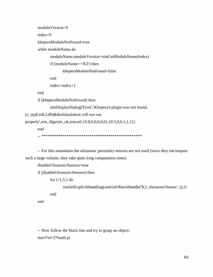
69
moduleVersion=0
index=0
kheperaModuleNotFound=true
while moduleName do
moduleName,moduleVersion=simGetModuleName(index)
if (moduleName=='K3') then
kheperaModuleNotFound=false
end
index=index+1
end
if (kheperaModuleNotFound) then
simDisplayDialog('Error','Khepera3 plugin was not found.
(v_repExtK3.dll)&&nSimulation will not run
properly',sim_dlgstyle_ok,true,nil,0.8,0,0,0,0,0,0.5,0,0,1,1,1)
end
-- ************************************************
-- For this simulation the ultrasonic proximity sensors are not used (since they encompass
such a large volume, they take quite long computation time):
disableUltrasonicSensors=true
if (disableUltrasonicSensors) then
for i=1,5,1 do
simSetExplicitHandling(simGetObjectHandle('K3_ultrasonicSensor'..i),1)
end
end
-- Now follow the black line and try to grasp an object:
maxVel=2*math.pi
70
-- Here is the execution of the regular thread code:
res,err=xpcall(threadFunction,function(err) return debug.traceback(err) end)
if not res then
simAddStatusbarMessage('Lua runtime error: '..err)
end
-- Put some clean-up code here:

71
LUA code used for final simulation that generated robots path when given angular
velocities at a given time interval. For this particular case the path was a parabola:
-- This script runs in a thread. A non-threaded script can also be used instead
-- Following commands are implemented:
--
-- distance_inMeters=simExtK3_getInfrared(index_of_ir_sensor_0_to_8)
-- distance_inMeters=simExtK3_getUltrasonic(index_of_us_sensor_0_to_5)
-- intensity_0_to_1=simExtK3_getLineSensor(index_of_line_sensor_0_to_1)
-- distance_inMeters=simExtK3_getGripperProxSensor(index_of_finger_prox_sensor_0_to_1)
-- simExtK3_setVelocity(velocityLeft_radPerSec,velocityRight_radPerSec)
-- simExtK3_setArmPosition(position_300_to_900)
-- simExtK3_setGripperGap(gap_0_to_170)
threadFunction=function()
while simGetSimulationState()~=sim_simulation_advancing_abouttostop do
t = <insert data for time intervals>
OmegaL = <insert data for left wheel angular velocity here>
OmegaR = <insert data for right wheel angular velocity here>
for a= 1, 903, 1 do
while t[a] > simGetSimulationTime() do
velLeft = OmegaL[a]
velRight = OmegaR[a]
simExtK3_setVelocity(velLeft,velRight)
end

72
end
while (simExtK3_getInfrared(1) ~= 100 or simExtK3_getInfrared(2) ~= 100 or
simExtK3_getInfrared(3) ~= 100 or simExtK3_getInfrared(4) ~= 100) do
if (simExtK3_getInfrared(1)< 3) then
velLeft=maxVel
velRight=-maxVel
simWait(math.pi/6)
elseif (simExtK3_getInfrared(2)< 5) then
velLeft = maxVel
velRight = -maxVel
simWait(math.pi/4)
elseif (simExtK3_getInfrared(3)< 5) then
velLeft = -maxVel
velRight = maxVel
simWait(math.pi/4)
elseif (simExtK3_getInfrared(4)< 3) then
velLeft = -maxVel
velRight = maxVel
simWait(math.pi/6)
end

73
simExtK3_setVelocity(velLeft,velRight)
end
simExtK3_setVelocity(velLeft,velRight) -- Set desired left and right motor
velocities
end
end
-- Put some initialization code here:
-- Check if the required plugin is there:
-- ************************************************
moduleName=0
moduleVersion=0
index=0
kheperaModuleNotFound=true
while moduleName do
moduleName,moduleVersion=simGetModuleName(index)
if (moduleName=='K3') then
kheperaModuleNotFound=false
end
index=index+1
end
if (kheperaModuleNotFound) then
simDisplayDialog('Error','Khepera3 plugin was not found.
(v_repExtK3.dll)&&nSimulation will not run
properly',sim_dlgstyle_ok,true,nil,0.8,0,0,0,0,0,0.5,0,0,1,1,1)
end
-- ************************************************
74
-- For this simulation the ultrasonic proximity sensors are not used (they encompass such a large
volume, they take quite long computation time):
disableUltrasonicSensors=true
if (disableUltrasonicSensors) then
for i=1,5,1 do
simSetExplicitHandling(simGetObjectHandle('K3_ultrasonicSensor'..i),1)
end
end
-- Now follow the black line and try to grasp an object:
maxVel=2*math.pi
-- Here is the execution of the regular thread code:
res,err=xpcall(threadFunction,function(err) return debug.traceback(err) end)
if not res then
simAddStatusbarMessage('Lua runtime error: '..err)
end