Storm Water Best Management Practices (BMPs)

Field Trials of Erosion Control Compost in

Reclamation of Rock Quarry Operations

Final Report to:

Nonpoint Source Protection Program CWA §319(h)

Texas Commission on Environmental Quality

Prepared by

Todd Adams, Anne McFarland, and Larry Hauck

Texas Institute for Applied Environmental Research

Tarleton State University

Stephenville, Texas

and

Michael Barrett and Brad Eck

Center for Research in Water Resources

The University of Texas

Austin, Texas

August 2008

PR 0804

PREPARED IN COOPERATION WITH THE TEXAS COMMISSION ON ENVIRONMENTAL QUALITY AND

U.S. ENVIRONMENTAL PROTECTION AGENCY

The preparation of this report was financed through grants from the U.S. Environmental Protection Agency through the Texas Commission on Environmental Quality.

ii

Table of Contents

1 Introduction................................................................................................................. 1

2 Literature Review........................................................................................................ 3

3 Materials and Methods................................................................................................ 7

3.1 Field Installation................................................................................................... 7

3.2 Compost Testing ................................................................................................ 11

3.3 Water Sample Collection and Laboratory Analysis........................................... 13

3.4 Soil Collection and Analysis .............................................................................. 14

3.5 Vegetation and Erosion Monitoring................................................................... 14

3.6 Runoff Data Analysis ......................................................................................... 14

4 Results and Discussion ............................................................................................. 17

4.1 Overview ............................................................................................................ 17

4.2 Compost and Soil Testing .................................................................................. 17

4.3 Vegetation .......................................................................................................... 20

4.4 Runoff Volume................................................................................................... 23

4.5 Runoff Concentrations ....................................................................................... 31

4.5.1 Variation within and between Treatments over Time................................. 31

4.5.2 Comparisons between Treatment for Paired Event Concentrations ........... 40

4.6 Nutrient and Sediment Loads............................................................................. 42

4.7 Impacts on Receiving Waters............................................................................. 46

5 Conclusions............................................................................................................... 50

6 References................................................................................................................. 53

Appendix A: Monthly and Bimonthly Pictorial Observations ..........................................56

Appendix B: Observed Runoff Volumes and Concentrations.........................................133

Appendix C: Monthly and Bimonthly Narrative Observations .......................................146

Appendix D: Statistical Details........................................................................................159

iii

List of Tables

Table 3-1 Erosion Control Treatments ............................................................................. 10

Table 3-2 Analysis Methods and Reporting Limits for Compost and Soil Parameters.... 12

Table 3-3 Laboratory Analysis Methods .......................................................................... 13

Table 4-1 Analysis of Compost Conducted by TSU/TAES Compost Analysis Laboratory

using TMECC methods..................................................................................................... 18

Table 4-2 Analysis of Compost and Compost-Blend Samples Conducted by TIAER

Laboratory......................................................................................................................... 18

Table 4-3 Soil analysis results for 0-6 inch samples collected annually. ......................... 19

Table 4-4 Monthly Vegetative Cover Estimated as Percent of Plot ................................. 21

Table 4-5 Storm Events with Volume or Water Quality Data.......................................... 24

Table 4-6 Multiple Regression Summary by Treatment for Equation 1 .......................... 26

Table 4-7 Projected Runoff Volumes for Events Not Measured...................................... 28

Table 4-8 Estimated Total Runoff Volume ...................................................................... 31

Table 4-9 Average Concentrations (mg/L) ....................................................................... 38

Table 4-10 Prevailing Conditions and Mean Concentrations at Steady State .................. 39

Table 4-11 P Values from Paired t Testing....................................................................... 40

Table 4-12 Comparison of Total Load for All Events, June 2006-May 2008.................. 43

Table 4-13 Applied and Exported Nutrients..................................................................... 46

Table 4-14 Range of literature values for nutrient export coefficients. ............................ 48

Table 4-15 Derived nutrient export coefficients from study plots.................................... 48

iv

List of Figures

Figure 3-1 Potential installation site ................................................................................... 7

Figure 3-2 Construction of Test Plots................................................................................. 8

Figure 3-3 Test Plots with Runoff Collection System and Rain Gauge ............................. 9

Figure 3-4 Schematic of Test Plot Installation ................................................................. 10

Figure 3-5 Installation of Erosion Control Compost ........................................................ 11

Figure 4-1 Soil test values and 95 percent confidence intervals by treatment and year ... 20

Figure 4-2 Vegetative Cover (average of replicate plots) over time ................................ 21

Figure 4-3 Example of vegetation encroachment ............................................................. 23

Figure 4-4 Illustrative rainfall-runoff relationship for varying rainfall depths assuming

storms occurred halfway through the monitoring period with the median observed

precipitation intensity........................................................................................................ 26

Figure 4-5 Regression coefficients for rainfall slope and 95 percent confidence intervals

........................................................................................................................................... 28

Figure 4-6 Average TSS Concentrations .......................................................................... 32

Figure 4-7 Average TKN Concentrations and Outlier Concentrations ............................ 33

Figure 4-8 Average Nitrate Concentrations and Outlier Concentrations.......................... 34

Figure 4-9 Average Total N Concentrations..................................................................... 35

Figure 4-10 Average Dissolved Phosphorus Concentrations and Outlier Concentrations36

Figure 4-11 Average Total Phosphorus Concentrations and Outlier Concentrations....... 37

Figure 4-12 Average Loads of Dissolved P...................................................................... 45

1 Introduction

Citizens in Texas have recently expressed concern about the amount of sediment and

other constituents being conveyed to receiving waters in stormwater runoff from quarries.

Quarries include a variety of disturbed areas that are often almost completely lacking in

vegetation including active mining areas, process areas, spoils piles, and locations that

were previously sedimentation ponds used to treat process water. Runoff from areas of

bare soil, such as these, can convey extremely large amounts of suspended solids

compared to other rural land uses. Consequently, the Texas Commission on

Environmental Quality (TCEQ) initiated this project to evaluate various methods for

stabilizing disturbed areas at quarry sites.

In addition to quarries, areas disturbed by construction activities also generate large

amounts of sediment during storms, which leads to very visible impacts on nearby

surface waters. To protect these waters, the United States Environmental Protection

Agency (USEPA), through the Construction General Permit, requires disturbed areas to

be vegetated and stabilized before a Notice of Termination can be submitted to

regulators. Establishing vegetation proves to be time consuming and expensive on many

projects. To this end, research has shown that compost applied to disturbed lands

substantively reduces sediment loss and enhances vegetation establishment (Bresson et

al., 2001; Block, 2000).

Composting is the aerobic biological degradation of waste in the solid state (Rittman and

McCarty, 2001). In recent years, composting has become popular for dairy manure,

poultry litter, and wastewater treatment biosolids. The composting process consumes

biodegradable organic matter and releases carbon dioxide among other products. Due to

the destruction of organic matter and the associated reduction in volume, compost has

higher phosphorus concentrations than the original waste material (Sharpley and Beegle,

2001). The reduced volume makes the compost less costly to transport, but the higher

phosphorus concentrations in the compost may leach into runoff, potentially impairing

the quality of receiving waters (Easton and Petrovic, 2004). 1

The Texas Department of Transportation (TxDOT) has used compost on construction

projects since 1998 (Cogburn, 2007), and currently uses two specifications (161 &

Special 1001) for compost in erosion control applications. Both specifications blend

equal volumes of wood chips and compost to create Erosion Control Compost (ECC) for

application to disturbed areas, but differ in the organic content of the compost.

Specification 161 requires compost containing 25 percent - 65 percent organic matter by

mass, while Special Specification 1001 allows organic content as low as 10 percent by

mass for manure compost (TxDOT, 2004).

The aim of this study was to compare the vegetation establishment, runoff volume, and

water quality of the two types of TxDOT approved compost with a common industry best

management practice (BMP), wood based hydromulch, and a seeded bare soil control.

These four treatments were applied to test plots. Vegetation density and runoff volume

were sampled on selected occasions throughout the year. Runoff was analyzed for five

water quality parameters: total suspended solids (TSS), total Kjeldahl nitrogen (TKN),

nitrite-nitrogen plus nitrate-nitrogen (henceforth referred to as nitrate), dissolved

phosphorus as orthophosphate-phosphorus (dissolved-P), and total phosphorus (total-P).

Sampled events provided the basis for a comparison between treatments of the annual

runoff volume and mass loss of each water quality constituent.

2

2 Literature Review Previous studies evaluating the effect of compost on water quality and vegetation

establishment may be categorized according to the compost source material, how

precipitation was applied (natural or simulated), and the type of test area. Test areas have

included columns and trays of various sizes as well as field studies.

Bresson et al. (2001) compared erosion from a compost amended soil with a control soil

using simulated rainfall over small trays, none of which had vegetation. Test soils were

compacted into 50 x 50 x 15 cm test trays such that the bulk density ranged from 1,000 to

1,200 kg/m3. The trays were set at a 5 percent slope. Simulated rainfall was applied at

19 mm/h for 60 minutes, corresponding to a 3-year return period for the study area near

Paris, France. Runoff was collected continuously during rainfall simulation. The

compost amended soil delayed the onset of runoff from 2.5 to 9.2 mm of cumulative

rainfall. The average TSS concentration in the incipient runoff was 11,000 mg/L and

36,400 mg/L for the amended and control soils, respectively. Total sediment load was

18.3 g or 732 kg/ha for the amended soil and 54.6 g or 2184 kg/ha for the control soil.

Kirchoff et al. (2003) analyzed leachate from compost filled columns subjected to

simulated rainfall. Several blends of compost were studied; the results summarized here

pertain to erosion control compost from dairy manure. Rainfall was applied on eight

occasions such that the total rainfall was equivalent to the annual average rainfall for

Austin, Texas (31.5 inches or 800 mm). Nitrate and total nitrogen concentrations in

leachate decreased by an order of magnitude between the first and second rainfall

applications. In subsequent rainfall applications, concentrations stabilized around 2.5

mg/L for nitrate and 8.6 mg/L for total nitrogen. Total phosphorus concentrations were

relatively stable at around 3.3 mg/L throughout the study.

Kirchoff et al. (2003) also investigated erosion control properties of compost. A

precipitation depth of 67 mm was applied to a 275 x 91 cm test tray as the hyetograph of

a 2-year, 3-hour storm for Austin, Texas. Runoff from the tray was monitored

continuously. Compared to the clay loam control soil, the runoff hydrograph for the 3

dairy compost was flatter and shifted to the right. This result indicates that dairy compost

delays the onset of runoff and reduces the peak flow rate. A water quality analysis of one

sample contained the following concentrations: nitrate-N 0.73 mg/L, TKN 8.98 mg/L,

total-P 4.17 mg/L, and TSS 645 mg/L.

Easton and Petrovic (2004) performed a two year field study to determine the effect of

nutrient source on turfgrass runoff and leachate under natural rainfall. Fertilizers were

applied to 1 x 2 m plots situated on a 7-9 percent slope. Treatment plots received

repeated applications of fertilizer, totaling 100 or 200 kg-N/ha for the two year study.

Three organic composts were investigated (dairy, swine, and biosolids) with results

presented as the average of the three. Test plots experienced 33 precipitation events

totaling 536 mm. Nitrate concentrations in runoff generally decreased with time, but

appear to be influenced by repeated fertilizer application. Nitrate concentrations ranged

from 13 mg/L for the unfertilized control plot in the second month to 0.1 mg/L for the

compost plots in month 17. Nitrate concentrations in runoff from the treatments were

significantly different, with the control plot producing the highest concentrations.

Concentrations of phosphate (PO43--P) in compost runoff fluctuated between 0.1 and 1.5

mg/L, but exceeded 2.5 mg/L on two occasions following fertilizer application.

Phosphate concentrations from the control plots appeared fairly stable and averaged 0.3

mg/L and 0.5 mg/L for years 1 and 2, respectively. The study found that nutrient

concentrations and mass losses were highest in the 20-week period following turfgrass

seeding, with compost treatments having greater phosphorus loss on a percent applied

basis. The nutrient losses declined significantly once turfgrass cover was established.

The reduced nutrient runoff was related to overall plant growth and shoot density.

Faucette et al. (2004) studied the runoff from several composts and mulch blankets under

simulated rainfall. Composts used for the project were derived from poultry litter,

municipal solid waste, biosolids, food waste, and yard waste. The treatments were placed

into a 92 x 107 cm frame on a 10 percent incline. Rainfall was applied at 160 mm/hr for

one hour. This storm event exceeds the 1-hour, 100-year storm event for Athens,

Georgia. Solids loss from composts were less than bare soil, ranging from 111 g for yard

4

waste compost to 552 g for poultry litter compost, compared with 646 g for bare soil.

Losses of nitrogen and phosphorus from most of the compost treatments were higher than

those from bare soil or mulch treatments.

Xia et al. (2007) studied the leaching of nitrogen and phosphorus from compost filled

columns subjected to simulated rainfall. Rainfall was applied at 20.4 mm/hr for 100 min.

For one month, 10 of these events were conducted every other day such that the total

amount of water leached was equivalent to 25 percent of the mean annual rainfall in Fort

Pierce, Florida. Compost for this study consisted of a 1:1 mix of biosolids and yard

waste. Over the study period, nitrate concentrations dropped from 2000 mg/L to near 0

mg/L. Concentrations of total dissolved P in leachate rose from 10 mg/L to 35 mg/L

before declining to around 28 mg/L. Concentrations of phosphate in leachate rose from

10 mg/L to 30 mg/L before declining to 25 mg/L.

In addition to the experimental results presented above, other authors (Block, 2000;

Goldstein, 2002) have summarized compost demonstration projects from around the

USA. Block (2000) summarizes projects in Texas and Connecticut where compost

helped establish vegetation in resistant or difficult areas. The Connecticut study applied

different rates of compost to test plots. Compared to a control plot, the compost

significantly improved turf establishment. Differences among the treated plots were

subtle, suggesting that a small amount of compost helped establish vegetation. Four

demonstration projects in Texas showed that compost blended with wood chips could

establish vegetation in areas where other methods were unsuccessful. Goldstein (2002)

summarizes three studies of compost for erosion control and observes that “Positive

results are also found when establishing vegetation on a slope with seeded compost.”

In summary, previously published studies indicate that:

• Compost can help establish vegetation in difficult locations (Block, 2000;

Goldstein, 2002)

• Compost reduces sediment loss in runoff (Bresson et al., 2002; Faucette et al.,

2004) and reduces peak discharge (Kirchoff et al., 2003).

5

• Nitrate concentrations in leachate or runoff from composted areas tend to

decrease dramatically after the initial rain event before stabilizing. (Kirchoff et al.,

2003; Xia et al., 2007; Easton and Petrovic, 2004).

• Total phosphorus and phosphate observations did not exhibit a readily apparent

trend. Kirchoff et al. (2003) observed relatively constant phosphorus levels in

leachate, while Xia (2007) observed increasing concentrations. Easton and

Petrovic (2004) observed decreasing phosphorus concentrations in leachate, but

varying concentrations in runoff because of repeated fertilizer application.

Faucette et al. (2004) found that phosphorus losses in runoff from compost plots

were higher than mulch treatments or bare soil.

6

3 Materials and Methods

3.1 Field Installation

Test plots for this project were constructed on the property of Vulcan Materials Company

in southwest Parker County, Texas. The Texas Institute for Applied Environmental

Research (TIAER) at Tarleton State University coordinated plot installation, sample

analysis, and data collection with the company. Several sites within the quarry were

considered for test plot construction. Several of the possible locations were very steep,

making installation of treatments and monitoring equipment difficult (Figure 3-1).

Figure 3-1 Potential installation site

Ultimately, a site with more accessible terrain was selected for test plot installation. Plots

were 40 feet long and 8 feet wide and had an average slope of 12 percent. The plot

orientation and size were selected to encourage formation of erosive features such as rills

7

that might distinguish the erosion control treatments. Plots were also sized to balance the

runoff volume with the size of a readily available livestock water tank. To estimate the

volume of runoff, plots were assumed to have an SCS curve number of 88, which is

appropriate for pasture or rangeland with little vegetation coverage and underlain with

silty clay soils.

The quarry staff at Vulcan provided assistance in construction of test plots and in various

other areas of this project. Contributions of quarry personnel time, labor, and expertise

were instrumental to the overall success of the project. These contributions included

assistance in site selection, transportation of overburden to the test plot area, test plot

grading (Figure 3-2), formation of earthen berms between each plot and above the plot

area to isolate runoff, periodic site access repairs, watering of plots to aid vegetative

establishment during the first few months, and arrangement of on-site meetings and tours.

Coordination of these endeavors with quarry staff was effortless as quarry personnel were

very supportive of the project and willing participants.

Figure 3-2 Construction of Test Plots

8

Each plot was equipped with a runoff collection system consisting of a gutter and tank.

A 6-inch PVC pipe was cut lengthwise to function as a gutter. Metal flashing prevented

water from flowing under the gutter. Flow from the gutter was collected in a 160 gallon

livestock water tank. Prior to installation, the relationship between depth and volume for

each tank was calibrated by measuring the depth associated with a known volume of

water. A tipping bucket rain gauge recorded every time 0.01 inches of rainfall

accumulated in the gauge. Figure 3-3 shows the overall installation.

Figure 3-3 Test Plots with Runoff Collection System and Rain Gauge

Three different erosion control treatments were applied in May 2006 to eight of the 10

test plots, with two plots left untreated for experimental control. Treatments were

assigned to plots as shown in Figure 3-4. Two treatments utilized a 1:1 blend of

composted dairy manure and wood mulch. One of these treatments utilized compost with

relatively low organic matter (OM) content consistent with TxDOT Special Specification

1001, while the other utilized compost with higher OM content in accordance with

TxDOT Specification 161. The third treatment consisted of Biocover Daily Landfill

hydromulch, manufactured by Profile Products LLC. Table 3-1 summarizes the

composition and nutrient content of the erosion control treatments

9

Table 3-1 Erosion Control Treatments

Composition Treatment

Application Rate

(kg/ha)

Total Nitrogena (kg/ha)

Total Phosphorusa

(kg/ha) Wood Fiber Other

Low OMb 282,454c 1375 585 50%

50% composted dairy manure

(12.8% organic matter)d

High OMe 282,454c 3249 1565 50%

50% composted dairy manure

(29.6% organic matter)d

Hydromulch 2,242 18 22 67% 20% corrugated

carton fiber, 10% Tackifier

a Nutrients in compost-blend based on laboratory analysis. Nutrients in hydromulch based on information from the manufacturer on the addition of liquid fertilizer. b Organic content meets TxDOT specification 1001. c Assumes compost-blend applied at a rate of 141 kg/ha (126 ton/acre) based on 2.5 cm (1-inch) compost and 2.5 cm (1-inch) wood chips. d TSU/TAES Compost Analysis Laboratory using TMECC methods e Organic content meets TxDOT special specification 161.

Figure 3-4 Schematic of Test Plot Installation

The designated treatment was blown onto compost-treated plots using a hose (Figure

3-5). The compost treated plots were then hand seeded with grass and lightly raked to

10

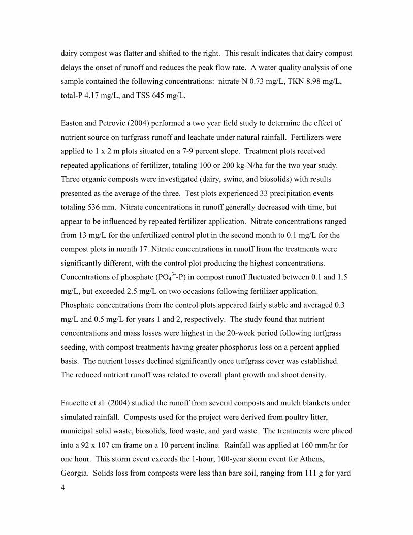
incorporate the seed. The hydromulch plots were hand seeded with grass prior to

treatment application. Ernie Parker of Finish Line Supply applied the hydromulch. All

plots were seeded with Giant bermudagrass (Cynodon dactylon, var. aridus) at a rate of

17.6 kg/ha and Common bermudagrass (Cynodon dactylon) at a rate of 6.4 kg/ha.

Figure 3-5 Installation of Erosion Control Compost

3.2 Compost Testing

Compost installed on test plots was analyzed in accordance with requirements for use by

the TxDOT. Two compost samples were analyzed for percent organic matter, total

nitrogen (total- N), and total phosphorus (total-P) by the Tarleton State University/Texas

Agriculture Extension Service (TSU/TAES) Compost Analysis Laboratory following

certified Test Methods for the Examination of Composting and Compost (TMECC)

methodology (Table 3-2). The TSU/TAES Compost Analysis Laboratory participates in

the United States Composting Council (USCC) Seal of Testing Assurance program. The

11

two compost samples were also analyzed by the TIAER Laboratory for percent organic

matter, total Kjeldahl nitrogen (TKN), extractable nitrate nitrogen (Ext-NO3-N), total-P,

and Mehlich III extractable phosphorus (ext-P) in order to provide consistency between

the methods used and results obtained for the compost and soil testing portions of the

project. Two additional samples were collected after blending of the compost with

mulch. These blended-compost samples were only analyzed by the TIAER Laboratory.

Table 3-2 Analysis Methods and Reporting Limits for Compost and Soil

Parameters.

Parameter Method a Reporting Limit b Laboratory Matrix

Organic Matter (%) TMECC 05.07A 0.1 TSU/TAES Compost Total Nitrogen (mg/kg) TMECC 04.02D 20 TSU/TAES Compost

Total Phosphorus (mg/kg) TMECC 04.03A 4 TSU/TAES Compost Organic Matter (%) SM2540G 1.0 TIAER Compost and Soil

Total Kjeldahl Nitrogen (mg/kg) EPA 351.2 modified c 2.0 TIAER Compost and Soil

Total Phosphorus EPA 365.4 modified c 1.0 TIAER Compost and Soil Extractable Nitrate (mg/kg) EPA 353.2 d 0.5 TIAER Compost and Soil

Extractable Phosphorus (mg/kg) EPA 365.2 c 0.1 TIAER Compost and Soil

a TMECC refers to Test Methods for the Examination of Composing and Compost (TMECC, 2004), SM refers to Standard Methods for the Examination of Water and Waste Water (APHA, 1998), and EPA refers to USEPA Methods for Chemical Analysis of Water and Wastewater (USEPA, 1983). b Reporting limits for solids are estimated on percent dry solids. All soil and compost parameters are reported on a dry weight basis as calculated. c Modification of the TKN and TP methods involves using copper sulfate as the catalyst instead of mercuric sulfate. d Extraction procedures for NO3-N (deionized water) and P (Mehlich III) follow Soil Science Society of America, Methods of Soil Analysis (SSSA, 1996).

The following protocol was followed for field sampling of compost and the compost-

blend. Using a collection device (e.g., hand trowel or spade), at least 15 representative

samples were collected from the compost pile and placed in a plastic bucket.

Representative composite sampling of blended stockpile was conducted per TMECC

Method 02.01-A, “Compost Sampling Principles and Practices.” After thorough mixing,

a composite sample of the compost was taken from the bucket, placed in a plastic bag

(labeled with date, time, and sample pile), and stored in an iced chest for transport to the

TIAER Laboratory. Of note, the compost-blend samples were collected from the

applicator hose during treatment installation to ensure quality control. Splits of the

12

compost samples were analyzed by the two laboratories, while the compost-blend was

analyzed only by the TIAER laboratory.

3.3 Water Sample Collection and Laboratory Analysis

All storm events were monitored for runoff volume and TSS during the first few months

after treatment application. Beginning September 1, 2006, the monitoring strategy was

altered to only sample events when there was sufficient runoff from all 10 plots to

conduct the required chemical analyses. In late November 2006, due to the larger than

expected number of events that had occurred to date, the monitoring strategy was further

amended to sample only one event (where all 10 plots responded) every two months

starting January 2007. These modifications were necessary to spread out the 16 budgeted

events over the project to track changes over time as well as differences between

treatments.

Upon completion of a storm event selected for sampling, TIAER personnel tabulated the

rainfall depth and runoff volume and collected a water sample. Stock tanks were covered

between storms to prevent contamination. The TIAER lab analyzed water samples to

determine the concentration of the following water quality parameters: TSS, nitrate,

TKN, dissolved-P, and total-P. Table 3-3 provides a detailed listing of the laboratory

methods utilized for this project.

Table 3-3 Laboratory Analysis Methods

Parameter EPA Methoda AWRLb RLc

Total Suspended Solids (TSS) 160.2 4 4 Nitrate-plus-nitrite as nitrogen, dissolved, lab filteredd (nitrate) 353.2 0.04 0.04

Total Kjeldahl Nitrogend (TKN) 351.2 (modified)e 0.02 0.02 Orthophosphate Phosphorus, dissolved, lab filteredd (dissolved P) 365.2 0.04 0.005

Total Phosphorusd (total P) 365.4 (modified)e 0.06 0.06 a USEPA (1983) b AWRL = Ambient Water Reporting Limit c RL = Reporting Limit d Due to the amount of sediment in the samples, all samples were filtered and preserved, as necessary, in the TIAER lab. e Method modified to use copper sulfate as the catalyst instead of mercuric sulfate

13

3.4 Soil Collection and Analysis

Soil samples were collected annually from each plot and represent a depth of 0-6 inches

from the surface using a standard soil probe. When soil samples were collected, any

treatment material (compost or hydromulch) or vegetation was scraped aside prior to

inserting the soil probe. Ten 0-6 inch soil plugs were taken randomly within each plot

and composited to represent the soil sample for a plot. Soil parameters evaluated

included percent organic matter (OM), total Kjeldahl nitrogen (TKN), extractable nitrate

nitrogen, total phosphorus (TP), and extractable phosphorus (ExtP) as outlined in Table

3-2. An initial set of soil samples was collected June 8, 2006 after treatment installation.

The second set was collected June 18, 2007 and the third set April 17, 2008.

3.5 Vegetation and Erosion Monitoring

Narrative and digital photographic documentation of the test plots during installation and

at least once per quarter afterward were used to document visible evidence of the relative

success of the different BMP systems in establishing vegetation and in containing

erosion, sediment, and other nonpoint source pollution. Percent vegetation cover was

recorded at 30-day intervals based on visual observation (beginning within 60 days of

initial installation) until 70 percent cover was attained on both compost-treated BMP

systems and at 60-day intervals thereafter.

Encroachment of vegetation between plots was managed manually by installation of

metal edging and use of a gas powered trimmer (e.g. weedeater). The trimmer was used

to remove vegetation that had clearly encroached from an adjacent plot rather than grown

from within the plot itself. This approach to controlling encroachment was deliberately

selected over manually pulling-up the runners, or using an herbicide such as glyphosate.

3.6 Runoff Data Analysis

Analysis of storm runoff data focused on the following four areas:

• Comparison of runoff response between treatments and estimation of runoff

volumes for storms not monitored using multiple regression techniques, 14

• Evaluation of concentration data for outliers and changes in concentration over

time,

• Comparison of event concentrations between treatments using paired t-tests, and

• Estimation of treatment loadings.

The runoff response of each treatment was evaluated to determine the amount of rainfall

required to initiate runoff and the amount of rainfall retained by the treatment once runoff

began. This information was used to estimate runoff volumes for unmonitored events.

Estimation of runoff volume for storms not monitored was important for evaluating

overall runoff volumes and treatment loads. While the project was designed to monitor

only 16 rainfall-runoff events, nearly 65 inches of rainfall occurred of which only about

20 inches or 30 percent was monitored. Rainfall was measured throughout the project

using a tipping bucket rain gauge logging at one-minute intervals. Multiple regression

techniques were implemented to estimate runoff volume for events not monitored based

on the relationship of measured runoff volume for each treatment with rainfall depth,

time, and peak rainfall intensity for each treatment. Rainfall depth represented the total

rainfall associated with a runoff event. Time was defined as the number of days since the

first storm event. Rainfall intensity was computed on a 15 minute basis, with the peak

intensity being the maximum value for a given storm event. In some cases, runoff

overflowed the tank used for volume measurement. These overflow events were

excluded from the regression analysis. To compare derived coefficients between

treatments, 95 percent confidence intervals were calculated on the regression coefficients.

To initially assess water quality, concentrations were plotted over time to visually

observe changes between and within treatments, particularly with the establishment of

vegetation, and to determine outliers that should be removed prior to further data

analysis. Once outliers were determined, concentrations were averaged for plots within

the same treatment. It was anticipated that concentrations of runoff parameters would

stabilize over time. To determine if treatments obtained relatively stable runoff

concentrations, the time series of concentration for each water quality parameter was

divided into regions of changing and steady state concentration by visual inspection. A 15

regression line was fitted to data points within the hypothesized region of relatively

constant concentration. If the 95 percent confidence interval for the slope of the

regression included zero, indicating no significant relationship, the concentration was

considered steady state. The steady state concentration was reported as the average of

data points within that region representing the prevailing concentration after

establishment of vegetation. Where a stabilized region was not visually evident, no

steady-state regression was performed and no concentration was reported.

To compare runoff concentrations between treatments, paired t testing was applied to all

events. Treatments were compared based on the event average concentration of plots

representing each treatment with outliers removed. A p-value from a paired t test was

calculated for each pair of treatments, so that each water quality parameter had six p-

values. These p-values estimate the probability that observations come from the same

population. Treatment pairs with a p-value less than 0.05 were considered statistically

different.

Measured and estimated nutrient and sediment loadings were calculated for the study

period (June 2006 – May 2008) for measured and unmeasured rainfall events. For

measured events, the concentration was multiplied by the volume, except when overflow

was indicated. For unmeasured events, the runoff volume was estimated using the

multiple regression model based on rainfall depth, intensity and time since the first event.

Concentrations were linearly interpolated between sampled events based on the date of

the unmeasured event. Total loadings were calculated as the sum of measured and

unmeasured events.

16

4 Results and Discussion

4.1 Overview

This project required several types of measurements:

• Nutrient concentrations in soil and compost,

• Vegetation density,

• Rainfall depth and runoff volume, and

• Nutrient and suspended solid concentrations in runoff.

Each measurement relates to the mass of TSS or nutrient exported from the test plots. In

the following sections, the categories of data are presented independently. Runoff

volume and concentration data are combined to estimate the mass loss of each

constituent. The impact of nutrient losses on receiving waters is quantified by deriving

export coefficients (kg/ha/yr) for each nutrient and treatment.

4.2 Compost and Soil Testing

Nutrient levels were measured in the soil underlying test plots and of the compost applied

to treatments. Nutrient levels in compost relate to the amount of nutrient applied with an

erosion control treatment. Levels in soil relate to the nutrient available to all treatments.

The level of organic matter was also measured to investigate its relationship with

vegetative performance.

Compost alone was tested by two different laboratories. One lab used methods

specifically for compost testing, while the other lab used methods for testing soil (Table

3-2). Compost treatments (compost blended with wood mulch) were only tested by the

laboratory that used the soil methods.

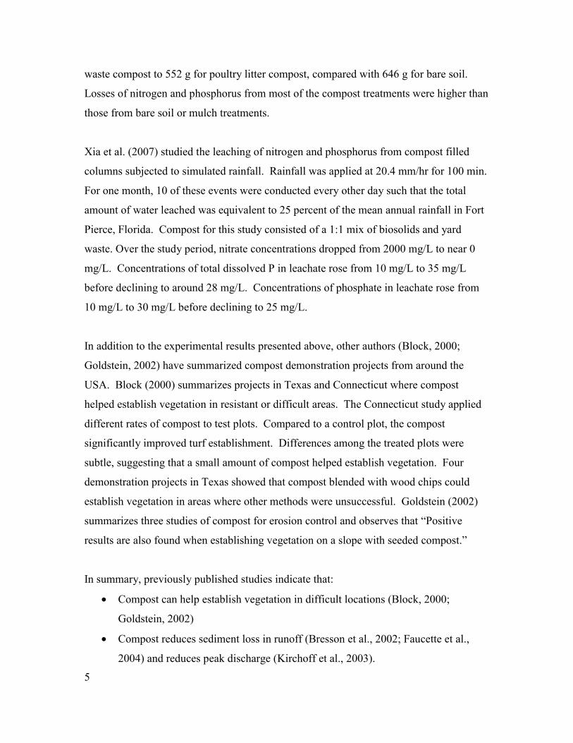
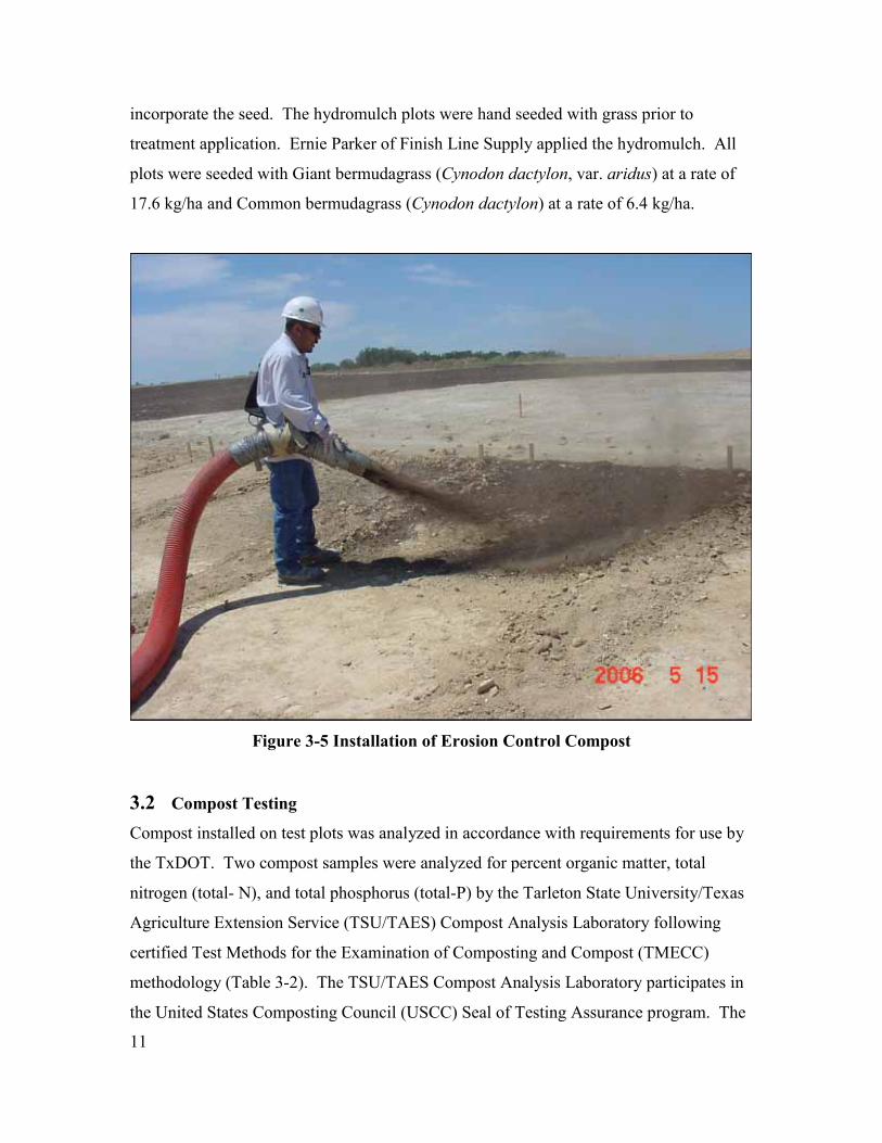
Analysis of compost samples prior to blending with mulch indicated desired values of

about 13 percent OM for the low OM compost and 30 percent OM for the high OM

compost following TMECC methods (Table 4-1). Total-N concentrations in the low OM

17

compost were about half that of the high OM compost, while total-P concentrations were

about a third as much in the low OM compost as in the high OM compost.

Table 4-1 Analysis of Compost Conducted by TSU/TAES Compost Analysis

Laboratory using TMECC methods.

Sample Description OM(%) Total-N (mg/kg)

Total-P (mg/kg)

Low OM Compost 12.8 7,100 2,380 High OM Compost 29.6 15,300 6,770

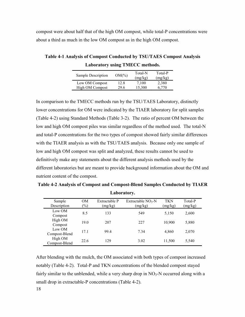
In comparison to the TMECC methods run by the TSU/TAES Laboratory, distinctly

lower concentrations for OM were indicated by the TIAER laboratory for split samples

(Table 4-2) using Standard Methods (Table 3-2). The ratio of percent OM between the

low and high OM compost piles was similar regardless of the method used. The total-N

and total-P concentrations for the two types of compost showed fairly similar differences

with the TIAER analysis as with the TSU/TAES analysis. Because only one sample of

low and high OM compost was split and analyzed, these results cannot be used to

definitively make any statements about the different analysis methods used by the

different laboratories but are meant to provide background information about the OM and

nutrient content of the compost.

Table 4-2 Analysis of Compost and Compost-Blend Samples Conducted by TIAER

Laboratory.

Sample Description

OM (%)

Extractable P (mg/kg)

Extractable NO3-N (mg/kg)

TKN (mg/kg)

Total-P (mg/kg)

Low OM Compost 8.5 133 549 5,150 2,600

High OM Compost 19.0 207 227 10,900 5,880

Low OM Compost-Blend 17.1 99.4 7.34 4,860 2,070

High OM Compost-Blend 22.6 129 3.02 11,500 5,540

After blending with the mulch, the OM associated with both types of compost increased

notably (Table 4-2). Total-P and TKN concentrations of the blended compost stayed

fairly similar to the unblended, while a very sharp drop in NO3-N occurred along with a

small drop in extractable-P concentrations (Table 4-2). 18

Soils underlying each treatment plot indicated very low extractable P and NO3-N

concentrations (Table 4-3). All extractable P concentrations were below 3 mg/kg and

except for the first year, extractable NO3-N concentrations were less than 2 mg/kg. On

the untreated and hydromulch plots, concentrations of TKN and total-P stayed essentially

constant over the study period (Figure 4-1). Mean TKN and total-P concentrations in the

soil under the compost treated plots doubled over the study period, though the increase

was not statistically significant due to the wide range of values measured in 2008.

Table 4-3 Soil analysis results for 0-6 inch samples collected annually.

Treatment Site Date Ext P (mg/kg)

Ext NO3-N (mg/kg)

TKN (mg/kg)

Total-P (mg/kg) OM (%)

Untreated VP04 6/8/2006 < 0.9a 9 390 233 1.4 6/18/2007 < 0.9 < 2b 540 239 2.7 4/17/2008 < 0.9 < 2 484 236 < 1.0c VP08 6/8/2006 < 0.9 11 423 227 3.0 6/18/2007 < 0.9 < 2 520 256 2.7 4/17/2008 < 0.9 < 2 507 271 < 1.0 High OM VP02 6/8/2006 < 0.9 9 453 238 1.8 6/18/2007 < 0.9 < 2 749 351 2.9 4/17/2008 1.1 < 2 644 297 < 1.0 VP06 6/8/2006 < 0.9 9 411 227 2.1 6/18/2007 < 0.9 < 2 634 310 3.0 4/17/2008 1.5 < 2 1053 453 1.1 Hydromulch VP03 6/8/2006 < 0.9 9 376 304 1.8 6/18/2007 < 0.9 < 2 620 359 2.7 4/17/2008 < 0.9 < 2 646 380 < 1.0 VP07 6/8/2006 < 0.9 12 498 328 2.2 6/18/2007 < 0.9 < 2 565 308 2.9 4/17/2008 < 0.9 < 2 626 298 < 1.0 VP10 6/8/2006 < 0.9 13 480 300 2.3 6/18/2007 < 0.9 < 2 578 327 2.8 4/17/2008 < 0.9 < 2 528 300 < 1.0 Low OM VP01 6/8/2006 < 0.9 15 576 294 2.2 6/18/2007 < 0.9 < 2 757 309 2.9 4/17/2008 < 0.9 < 2 709 272 < 1.0 VP05 6/8/2006 < 0.9 12 387 211 2.0 6/18/2007 < 0.9 < 2 659 306 3.0 4/17/2008 1.1 < 2 1024 400 1.1 VP09 6/8/2006 < 0.9 19 419 234 2.3 6/18/2007 < 0.9 < 2 763 279 3.2 4/17/2008 2.2 < 2 1506 507 1.4 a Measured values are less than the Ext P method detection limit of 0.9 mg/kg. b Measured values are less than the Ext NO3-N method detection limit of 2 mg/kg. c Measured values are less than the OM reporting limit of 1.0 %.

19

Figure 4-1 Soil test values and 95 percent confidence intervals by treatment and

year

Nutrients from the compost materials clearly are leaching into the soils increasing the

nutrient content of the underlying soil. While TKN and total P in the soils are increasing,

the extractable nutrient concentrations in year 3 were near or below the laboratory

reporting limit. The calcareous nature of the soils associated with the mining operation

tightly binds most phosphorus making it unavailable in runoff unless moved with eroded

sediment.

4.3 Vegetation

Vegetative cover was monitored throughout the study to see how quickly the different

treatments established vegetation. The fraction of vegetative cover was estimated on

thirteen occasions after treatments were established (Table 4-4 and Figure 4-2). Compost

plots established vegetation faster than other treatments, achieving complete (100

percent) cover in about four months.

20

Table 4-4 Monthly Vegetative Cover Estimated as Percent of Plot

Treatment and Plot Numbers Low OM High OM Hydromulch Untreated

Date 1 5 9 2 6 3 7 10 4 8 7/14/06 10 10 <10 10 <10 10 25 15 <1 0 8/14/06 20 20 10 15 15 10 25 15 <1 0 9/14/06 70 80 55 60 70 15 35 30 <1 0

10/14/06 100 99 100 100 100 30 50 60 <1 <1 12/14/06 100 100 100 100 100 45 65 75 1 1 2/21/07 100 100 100 100 100 45 65 75 1 1 4/19/07 100 100/99a 100 100 100/95a 45 70 75 1 1 6/18/07 100 100/99a 100 100 100/99a 95 99 99 10 20 8/20/07 100 100 100 100 100 100 100 100 50 80

10/16/07 100 100 100 100 100 100 100 100 95 100 1/3/08 100 100 100 100 100 100 100 100 95 100

2/14/08 100 100 100 100 100 100 100 100 95 100 4/17/08 100 100 100 100 100 100 100 100 95 100

a Represents percent coverage of new vegetative growth.

0

10

20

30

40

50

60

70

80

90

100

6/1/06 10/1/06 1/31/07 6/2/07 10/2/07 2/1/08 6/2/08

Veg

etat

ive

Cov

er (%

)

Avg LowOM Avg HighOM Avg Hydromulch Avg Untreated

Figure 4-2 Vegetative Cover (average of replicate plots) over time

Based on visual observation, the compost plots appeared to establish vegetation at the

same rate. However, visual observation cannot detect small differences in vegetation

density, so the two types of compost treatments may actually establish vegetation at 21

different rates. The hydromulch plots took almost three times longer than the compost

plots, establishing complete coverage after a year. Even after a year, the seeded bare soil

plots had little vegetation, which was consistent with the higher nutrient levels present in

the hydromulch and compost and agrees with observations of Bresson (2002). The

advantage of compost over hydromulch is that compost provides a better place for seeds

to germinate and retains more water (Kirchoff et al., 2003).

Harsh climactic conditions inhibited the vegetative establishment of all treatments during

the first summer of the study. Severe drought conditions existed from June 2006 through

August 2006, with less than 1 inch of rain during this period. Furthermore, extreme

temperatures were experienced during August 2006 with several days over 100ºF. Due

to drought conditions, supplemental watering of test plots was performed by Vulcan staff

throughout June, July, and August 2006 to help establish vegetation.

Rainfall events occurring in September and October 2006 substantially increased

vegetative growth on compost treated plots (see Appendix C – Monthly and Bimonthly

Narrative Observations for September/October 2006). This growth resulted in the

unanticipated encroachment of compost plot vegetation onto nearby hydromulch and

untreated plots. Metal landscape edging (about 4 inches in height) was installed between

each plot on April 19, 2007 to curtail the encroaching vegetation (Figure 4-3). Also,

beginning in June 2006, periodic grass trimming along the metal edging was performed

to help control runner advancement between each plot. These combined efforts proved to

be effective in controlling further vegetative encroachment between the plots.

22

Figure 4-3 Example of vegetation encroachment

4.4 Runoff Volume

The volume of runoff produced by each test plot was measured to determine the amount

of rainfall retained by each treatment, facilitate the computation of mass losses during

monitored events, and provide a basis for estimating runoff volumes for events that were

not monitored. During this project, the field site had 136 rain days with 65 inches of total

rainfall. Complete volume and water quality observations—nonzero data for each of the

10 plots—were collected from 16 storm events throughout the project. Partial data,

usually runoff volume, were measured for seven additional events. Table 4-5

summarizes average runoff volumes for the events for which data were collected.

Appendix B contains all the runoff volume and water quality data collected for this

project. Rainfall from events with complete data totaled 19.77 inches or 30 percent of the

total rainfall. Relatively large storms (> 1.9 inches) in September, October, and

November 2006 caused the runoff collection tanks to overflow, so runoff volume could

not be determined for those events.

23

Table 4-5 Storm Events with Volume or Water Quality Data

Date LowOM HighOM Hydromulch Untreated 6/17/2006 0.36 No 0 3 4 22 6/17/2006 1.23 Yes 77 94 124 152 6/23/2006 0.28 No 0 0 0 13 6/24/2006 0.40 No 2 2 37 54 7/4/2006 1.11 Yes 65 62 135 159

8/12/2006 0.11 No 0 0 0 3 8/14/2006 0.45 Yes 12 8 50 59 8/27/2006 1.25 Yes 40 19 140 154 9/3/2006a 2.68 No n/a n/a n/a n/a

9/17/2006a 1.92 Yes n/a n/a n/a n/a 10/10/2006 0.45 No 0 0 25 100 10/15/2006a 2.51 Yes n/a n/a n/a n/a 10/24/2006 0.26 No 0 0 8 7 11/5/2006a 2.56 Yes n/a n/a n/a n/a 1/3/2007 0.70 Yes 10 10 82 73

3/11/2007 0.59 Yes 2 2 19 21 4/30/2007 0.97 Yes 7 4 67 83 6/1/2007 0.76 Yes 2 2 59 76

10/22/2007 0.65 Yes 2 2 2 13 11/25/2008 1.78 Yes 9 9 60 135 2/15/2008 1.10 Yes 9 15 83 126 3/18/2008 1.37 Yes 9 14 115 144 4/9/2008 0.87 Yes 11 19 122 158

Total: 24.36 257 261 1132 1546 a Overflow event--volume not applicable (n/a)

For each treatment, the relationship between runoff and rainfall, time, and peak rainfall

intensity was explored using multiple regression. The regression analysis excluded

overflow events, but included data from the seven additional storms where only some but

not all 10 plots responded. The regression equations have the form

Runoff = A + B*Rainfall + C*Day Number + D*Peak Intensity Equation 1

where Runoff is the depth of runoff in inches,

Rainfall is the depth of rainfall in inches,

Day Number is the number of days since the first event to account for changing

vegetation coverage,

24

Peak Intensity is the peak rainfall intensity for a 15 minute period in inches per

hour, and

A, B, C & D are coefficients determined by the regression.

Equation 1 uses runoff depth which is calculated as the runoff volume divided by the plot

area. Using depth rather than volume facilitates comparisons between watersheds of

different sizes.

In Equation 1, the date and intensity terms can be thought of as adjustments to the

intercept. Once these terms are known, the multiple regression becomes a line in two

dimensions. Figure 4-4 shows results from the rainfall-runoff multiple regression

relationship for varying rainfall depths or storm sizes occurring halfway through the

monitoring period (day number = 332) with the median observed precipitation intensity

of 0.554 inches/hr. If the values for day number and rainfall intensity are changed, the

lines in Figure 4-4 would have the same slope, but move vertically depending upon the

date and the precipitation intensity input into the regression model.

The runoff characteristics of each treatment may be conceptualized as an initial

abstraction and a continuous abstraction. The initial abstraction is the rainfall depth after

which runoff begins. In Figure 4-4, the initial abstraction corresponds to the intersection

of the regression line for each treatment with the abscissa (x-axis). Since the compost

lines in Figure 4-4 move vertically with time, the initial abstraction also changes, though

changes with time were not significant for the hydromulch and untreated plots (Table

4-6). After 180 days, runoff from the compost plots begins after nearly 0.5 inches of

rainfall but after 540 days (18 months) requires 1 inch to initiate runoff. The hydromulch

and untreated plots had an initial abstraction of nearly 0.2 inches. These differences

matter because the median rainfall depth for this study was 0.31 inches. The compost

plots do not produce runoff for more than half of the storm events. Bresson et al. (2001)

and Faucette et al. (2004) also showed that compost delayed runoff compared to bare soil.

25

The continuous abstraction is the fraction of rainfall that becomes runoff after the initial

abstraction. In Figure 4-4, the continuous abstraction corresponds to the slope of the line.

Slopes associated with rainfall depth ranged from 0.22 for the low OM compost treatment

to 0.5 for untreated plots (Table 4-6). Even after the initial abstraction, a smaller volume

of runoff is expected from the compost plots than the other treatments, because the slope

of the line is flatter.

Low OM

High OM

Hydromulch

Untreated

0

0.1

0.2

0.3

0.4

0.5

0.6

0.7

0.8

0.9

1

0 0.5 1 1.5 2Rainfall (in)

Run

off (

in)

Figure 4-4 Illustrative rainfall-runoff relationship for varying rainfall depths

assuming storms occurred halfway through the monitoring period with the median

observed precipitation intensity

Table 4-6 Multiple Regression Summary by Treatment for Equation 1

Treatment Regression Coefficient or Statistic Low OM High OM Hydromulch Untreated

A (inches) -0.066 9 -0.080 2 -0.111 -0.154 B (no units) 0.215 0.207 0.341 0.500 C (inches) -0.000363 -0.000327 -0.000165a -0.0000917a D (hours) 0.0610 0.0739 0.189 0.187 Residual Standard Error 0.0573 0.0775 0.130 0.089

Adjusted R2 0.823 0.731 0.733 0.909 a Parameter estimate for the regression coefficient was not statistically significant at level 0.05

26

Also presented in Table 4-6 are the residual standard error and adjusted R2 values for the

regression analysis. The adjusted R2 estimates the fraction of variability in the data that

is accounted for by the model, after adjusting for the number of model parameters.

Adjusted R2 values ranged from 0.731 for the high OM plots to 0.909 for the untreated

plots. The residual standard error is a measure of how well the multiple regression

equation reproduces measured values. The low OM plots had the lowest residual

standard error (0.0573) of all treatments while the hydromulch plots had the highest

residual standard error (0.130).

One impact of a higher residual standard error is wider confidence intervals for the

regression coefficients. While the other variables were important in characterizing the

amount of runoff, rainfall depth was the primary variable driving the regression equation

results. The confidence intervals about the estimated regression coefficient for rainfall

depth (parameter B) are shown in (Figure 4-5). The widest confidence interval (Figure

4-5) and the highest residual standard error for the overall multiple regression equation

(Table 4-6) were indicated for the hydromulch treatment. The confidence intervals

shown in Figure 4-5 in part confirm that the compost plots offer similar runoff

performance because the confidence intervals overlap. The confidence intervals about

parameter B (rainfall depth) also indicate that the industry BMP (hydromulch) was not

statistically different from untreated plots or the compost plots for this parameter. It

should be noted however, that the small overlap of the hydromulch interval with the

compost and untreated plots represents a very small chance that the slope coefficients are

actually the same.

27 ils.

All of the regression coefficients were statistically significant (p<0.05) except for day

number (coefficient C) on the hydromulch (p=0.06) and untreated plots (p=0.21). The p-

value for hydromulch is very close to the cutoff value of 0.05, suggesting that the

treatment probably does produce less runoff as time passes and vegetation grows. The p-

value for untreated plots is further from the cutoff making any inferences difficult.

Additional statistical results regarding the multiple regression models are provided in

Appendix C: Statistical Deta

0.215 0.207

0.341

0.5

0.0

0.1

0.2

0.3

0.4

0.5

0.6

0.7

LowOM HighOM Hydromulch Untreated

Rai

nfal

l Slo

pe

Figure 4-5 Regression coefficients for rainfall slope and 95 percent confidence

intervals

The regression coefficients shown in Table 4-6 were used to project runoff volumes for

unmeasured events and those events during which the tanks overflowed. In some cases

the runoff volume measured for an overflow event (i.e., the volume of the tank) exceeded

the volume predicted by the regression equation, suggesting that the overflow was small.

The volume of the collection tank was used in these cases. Table 4-7 shows the

estimated runoff volume from each treatment for events where only rainfall was

recorded.

Table 4-7 Projected Runoff Volumes for Events Not Measured

Runoff Volume (gallons per plot) Date and Time Rainfall Began

Rainfall (inches)

Day Number

Peak 15 min. Intensity Low OM High OM Hydromulch Untreated

8/11/2006 15:52 0.07 56 NAa 0 0 0 0 9/1/2006 17:36 0.13 77 0.147 0 0 0 0

10/14/2006 11:11 0.18 119 0.24 0 0 0 0 11/29/2006 17:37 0.52 166 0.64 5 4 32 42

12/1/2006 9:22 0.08 167 0.126 0 0 0 0 12/19/2006 10:05 0.58 185 0.58 5 4 33 45 12/25/2006 5:27 0.01 191 NA 0 0 0 0 12/29/2006 5:43 0.59 195 0.528 4 3 32 44 1/12/2007 13:17 0.48 210 0.328 0 0 16 26

28

29

Runoff Volume (gallons per plot) Date and Time Rainfall Began

Rainfall (inches)

Day Number

Peak 15 min. Intensity Low OM High OM Hydromulch Untreated

1/17/2007 12:07 0.02 215 NA 0 0 0 0 1/18/2007 11:43 0.2 215 0.124 0 0 0 0 1/19/2007 5:45 0.97 216 0.131 14 12 42 67 1/21/2007 9:23 0.01 218 NA 0 0 0 0 2/1/2007 4:23 0.32 229 0.12 0 0 0 1 2/2/2007 8:54 0.01 230 NA 0 0 0 0

2/12/2007 6:22 0.13 240 0.084 0 0 0 0 2/24/2007 5:26 0.1 252 NA 0 0 0 0

3/22/2007 12:17 0.01 278 NA 0 0 0 0 3/23/2007 3:50 0.01 279 NA 0 0 0 0 3/26/2007 9:24 1.88 282 1.04 59 58 136 191 3/29/2007 5:16 2.28 285 1.44 81 81 178 245 4/7/2007 10:24 0.12 294 0.091 0 0 0 0 4/10/2007 1:28 0.02 297 NA 0 0 0 0

4/13/2007 16:28 0.33 301 0.52 0 0 10 16 4/17/2007 8:27 0.67 304 1.281 9 11 62 78 4/24/2007 9:01 2 311 1.638 70 70 166 224 5/2/2007 16:09 1.31 320 2.4 49 53 147 184 5/5/2007 10:16 0.01 322 NA 0 0 0 0 5/7/2007 7:56 0.05 324 NA 0 0 0 0 5/9/2007 1:46 0.22 326 0.22 0 0 0 0

5/9/2007 17:15 0.04 327 NA 0 0 0 0 5/10/2007 6:09 0.12 327 0.24 0 0 0 0

5/12/2007 14:03 0.38 330 0.843 0 0 25 33 5/14/2007 16:00 0.01 332 NA 0 0 0 0 5/24/2007 13:58 0.53 342 0.726 0 0 30 43 5/25/2007 15:26 1.51 343 1.08 40 40 110 154 5/26/2007 16:11 0.09 344 NA 0 0 0 0 5/27/2007 11:10 0.01 344 NA 0 0 0 0 5/29/2007 4:57 2.28 346 3.2 98 103 242 310 5/31/2007 0:22 0.06 348 0.162 0 0 0 0 6/3/2007 6:54 0.31 351 1.164 0 0 31 37

6/10/2007 22:04 0.02 359 NA 0 0 0 0 6/14/2007 0:48 0.02 362 NA 0 0 0 0

6/14/2007 12:42 0.52 362 0.42 0 0 17 30 6/15/2007 6:10 1.86 363 1.607 60 61 153 208

6/15/2007 22:19 0.35 364 0.46 0 0 7 15 6/16/2007 23:33 2.37 365 1.6 81 81 188 259 6/20/2007 3:20 0.49 368 0.373 0 0 13 25

6/21/2007 15:31 0.16 370 0.241 0 0 0 0 6/24/2007 18:36 0.03 373 NA 0 0 0 0 6/25/2007 10:43 0.01 373 NA 0 0 0 0 6/26/2007 5:32 2.73 374 1.333 93 92 202 285

6/27/2007 17:05 0.19 376 0.112 0 0 0 0 6/29/2007 16:48 0.81 378 1.34 10 12 71 93 7/1/2007 13:19 0.2 380 0.4 0 0 0 0 7/2/2007 13:08 0.27 381 0.463 0 0 1 7

30

Runoff Volume (gallons per plot) Date and Time Rainfall Began

Rainfall (inches)

Day Number

Peak 15 min. Intensity Low OM High OM Hydromulch Untreated

7/3/2007 11:01 0.35 381 0.68 0 0 15 23 7/4/2007 15:23 0.32 383 0.245 0 0 0 3 7/5/2007 13:59 0.02 384 0.01 0 0 0 0 7/8/2007 15:33 0.01 387 NA 0 0 0 0

7/23/2007 15:42 0.11 402 0.099 0 0 0 0 7/28/2007 16:55 0.04 407 NA 0 0 0 0

8/2/2007 7:40 1.12 411 1.4 22 24 93 126 8/17/2007 15:50 0.58 427 0.743 0 0 31 47 8/30/2007 18:31 0.09 440 NA 0 0 0 0 9/1/2007 14:28 0.36 442 0.702 0 0 14 23 9/2/2007 13:46 0.52 443 1.104 0 0 40 54 9/3/2007 14:17 0.19 444 0.61 0 0 0 3 9/4/2007 18:18 0.72 445 0.304 0 0 24 44 9/9/2007 20:14 0.02 450 NA 0 0 0 0 9/10/2007 8:46 1.85 450 1.16 47 48 133 189

9/18/2007 21:28 0.07 459 0.056 0 0 0 0 10/15/2007 5:25 0.43 485 0.62 0 0 15 26

11/22/2007 22:12 0.11 524 0.061 0 0 0 0 12/1/2007 10:15 0.01 532 NA 0 0 0 0

12/10/2007 17:50 0.01 542 NA 0 0 0 0 12/11/2007 6:42 0.22 542 0.12 0 0 0 0 12/12/2007 8:14 0.26 543 0.134 0 0 0 0

12/14/2007 15:19 0.1 546 0.031 0 0 0 0 12/26/2007 3:02 0.04 557 0.047 0 0 0 0 1/22/2008 11:12 0.01 584 NA 0 0 0 0 1/25/2008 1:40 0.18 587 0.28 0 0 0 0 1/26/2008 9:20 0.01 588 NA 0 0 0 0 2/12/2008 3:09 0.06 605 NA 0 0 0 0 2/17/2008 6:21 0.01 610 NA 0 0 0 0 3/3/2008 0:29 1.51 625 1.173 20 23 104 152 3/6/2008 9:37 0.19 628 0.224 0 0 0 0

3/6/2008 22:12 0.49 629 0.213 0 0 0 15 3/9/2008 20:49 0.32 632 0.405 0 0 0 5 4/4/2008 0:15 0.44 657 0.98 0 0 23 38

4/8/2008 21:06 0.52 662 0.662 0 0 16 34 Total: 40 768 780 2,452 3,444

a NA indicated not applicable. The rainfall event was less than 15 minutes.

The compost plots were projected to produce much less runoff than hydromulch or

untreated plots (Table 4-8). This result is consistent with the work of Bresson et al.

(2001), Kirchoff et al. (2003), and Easton and Petrovic (2004). The availability of

nutrients and ability of the compost material to hold water on the plots greatly aided the

speed with which vegetation was able to establish on the compost plots compared to the

hydromulch and untreated plots. Even when all 10 plots were totally vegetated, the

compost treated plots continued to have much lower runoff.

Table 4-8 Estimated Total Runoff Volume

Total Runoff Volume (gallons per plot) Fractional Difference from Untreated

LowOM HighOM Hydromulch Untreated LowOM HighOM Hydromulch Untreated

Observed 257 261 1,132 1,546 -83% -83% -27% 0%

Estimated 768 780 2,452 3,444 -78% -77% -29% 0%

Overflowsa 449 450 608 802 -44% -44% -24% 0%

Total 1,474 1,491 4,192 5,792 -75% -74% -28% 0% a runoff volume for overflow events is the larger of the estimated value or the tank volume

4.5 Runoff Concentrations

Like runoff volume, concentrations of the water quality parameters were measured to

detect differences between treatments and estimate mass losses. Trends in runoff

concentrations were also analyzed to estimate what nutrient levels might be expected in

the future.

4.5.1 Variation within and between Treatments over Time

Time series graphs of concentration for each constituent were used to visually evaluate

the data for outliers and to assess variations in concentration within and between

treatments over time. Time series plots represent the average concentration by event of

plots within the same treatment. Points identified as outliers were not used in calculating

the average for the treatment. Several points identified as outliers were associated with

rodent activity at the field site. In these cases it is thought that rodent excrement in the

collection tanks caused very high nutrient concentrations.

31

Average TSS concentrations from all plots tended to dramatically decrease with time

(Figure 4-6), although an increase was noted on the untreated and hydromuch plots in the

spring of 2007. These events occurred on April 30 and June 1, 2007, when vegetative

cover was notable (45 to 75 percent) on the hydromulch plots and barely existent (1

percent) on the untreated plots (Table 4-4). These two events also occurred after fairly

large unsampled rainfall events (see Tables 4-5 and 4-7). The April 30 event had 0.97

inches of rain, and occurred only six days after a 2-inch event (April 24) that was

unsampled. Similarly the June 1 event had 0.76 inches of rain , and occurred only three

days after a 2.28-inch event (May 29) that was unsampled. The fairly large unsampled

rainfall events prior to the sampled events probably helped create soil moisture conditions

leading to more sediment runoff from plots with less vegetation. Average TSS

concentrations were very high for untreated plots, reaching a maximum of 80,000 mg/L.

The second highest TSS concentrations occurred from the hydromulch treated plots. No

outliers were identified for event TSS concentrations by plots, so all measured values

were used in calculating average TSS concentrations by treatment.

0

10,000

20,000

30,000

40,000

50,000

60,000

70,000

80,000

90,000

6/1/06 9/29/06 1/27/07 5/27/07 9/24/07 1/22/08 5/21/08

Con

cent

ratio

n (m

g/L)

LowOMHighOMHydromulchUntreated

Figure 4-6 Average TSS Concentrations

32

For TKN, untreated plots tended to have the highest concentrations (Figure 4-7), although

all values generally decreased over time. Because fertilizer or nutrients were not applied

to the untreated plots, the TKN in runoff appears to have come from the organic content

of the soil. High concentrations of TKN were related to the high TSS values, particularly

for the untreated plots. Early in the study, the high OM compost plots had higher TKN

concentrations than the low OM compost plots, which was consistent with the higher

TKN concentrations in the high OM compost blend (11,476 mg/kg) compared with the

low OM compost blend (4,863 mg/kg). While obscured by the scale in Figure 4-7 by the

end of the study, the low OM plots exhibited slightly higher TKN concentrations. A few

TKN concentrations were excluded as outliers in association with events monitored in

October and November 2007. These outliers in October and November 2007 may have

been related to rodent activity noted within the plots. The inexplicably high TKN

concentration reported for an untreated plot in February 2008 was also excluded as an

outlier in calculating treatment averages.

0

20

40

60

80

100

120

6/1/06 9/29/06 1/27/07 5/27/07 9/24/07 1/22/08 5/21/08

Con

cent

ratio

n (m

g/L)

LowOM LowOM Outliers

HighOM High OM Outliers

Hydromulch Hydromulch Outliers

Untreated Untreated Outliers

Figure 4-7 Average TKN Concentrations and Outlier Concentrations

33

For nitrate, the variation in concentrations over time showed a different pattern than TKN

or TSS (Figure 4-8). After the first few events, nitrate concentrations tended to show an

increasing pattern over time, particularly for the compost treatments. The very high

nitrate concentration associated with the low OM compost treatment during the first

runoff event (Figure 4-8) is most likely related to the high amount of extractable nitrogen

measured in the compost (Table 4-2) and soil test values (Table 4-3). Initial soil test

values of nitrate were also slightly higher on two of the low OM plots (VP01 = 15.1

mg/kg and VP09 = 19.5 mg/kg), while the average across all plots was 11.8 + 3.5 mg/kg.

The low OM compost also had a higher extractable nitrate concentration (7.34 mg/kg)

than the high OM compost blend (3.02 mg/kg). These higher soil and compost nitrate

concentrations most likely explain this spike for the low OM treatment. Nitrate

concentrations excluded as outliers occurred in October 2007 were most likely caused by

rodent activity. As with TKN, the inexplicably high nitrate concentration reported for an

untreated plot in February 2008 was excluded as an outlier.

0.0

0.5

1.0

1.5

2.0

2.5

3.0

3.5

4.0

6/1/06 9/29/06 1/27/07 5/27/07 9/24/07 1/22/08 5/21/08

Con

cent

ratio

n (m

g/L)

LowOMHighOMHydromulchUntreatedHydromulch OutliersUntreated Outliers

Figure 4-8 Average Nitrate Concentrations and Outlier Concentrations

34

When nitrate and TKN concentrations were added together to calculate total-N (Figure 4-

9), the pattern of runoff concentrations was most similar to those for TKN (Figure 4-7).

Nitrate as a percent of total-N ranged from a high of about 10 percent for the compost

plots to about 3 percent for the untreated plots, so the dominance of TKN concentrations

as part of total-N was not unexpected.

0

10

20

30

40

50

60

6/1/06 9/29/06 1/27/07 5/27/07 9/24/07 1/22/08 5/21/08

Con

cent

ratio

n (m

g/L)

LowOMHighOMHydromulchUntreated

Figure 4-9 Average Total N Concentrations

Compost plots generally produced much higher dissolved phosphorus concentrations than

hydromulch or untreated plots (Error! Reference source not found.). Both compost

treatments exhibited two peaks in dissolved-P concentration in the first six month of

monitoring, while the other treatments showed a general decline. During the later part of

35

the monitoring, dissolved-P concentrations in runoff showed a general increasing trend

from the compost treatments, while concentrations from the untreated and hydromulch

plots showed more stable concentrations over time. Dissolved-P concentrations excluded

as outliers from the treatment averages occurred only in October 2007. As noted before,

rodent activity was noted as the most likely cause for these outliers.

0

1

2

3

4

5

6

7

8

6/1/06 9/29/06 1/27/07 5/27/07 9/24/07 1/22/08 5/21/08

Con

cent

ratio

n (m

g/L)

LowOMHighOMHydromulchUntreatedLow OM OutliersHydromulch Outliers

Figure 4-10 Average Dissolved Phosphorus Concentrations and Outlier

Concentrations

Total phosphorus concentrations demonstrated the combined effect of TSS and dissolved-

P because phosphorus sorbs to soil particles. Like TSS, total phosphorus concentrations

generally declined through the study period (Figure 4-11), although as with dissolved-P, a

general increase in total-P concentrations was shown for the low and high OM compost

treatments. Untreated plots often had the highest total-P concentrations in runoff,

36

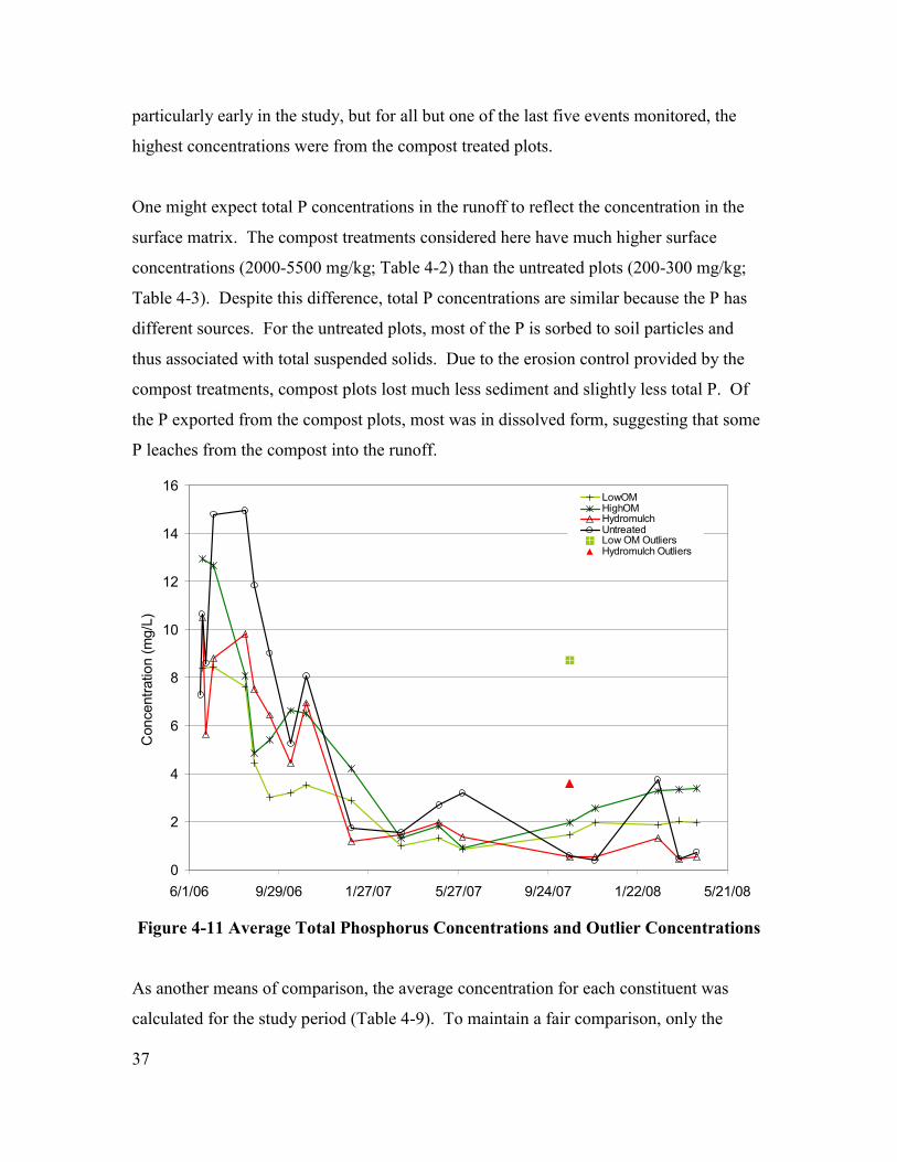
particularly early in the study, but for all but one of the last five events monitored, the

highest concentrations were from the compost treated plots.

One might expect total P concentrations in the runoff to reflect the concentration in the

surface matrix. The compost treatments considered here have much higher surface

concentrations (2000-5500 mg/kg; Table 4-2) than the untreated plots (200-300 mg/kg;

Table 4-3). Despite this difference, total P concentrations are similar because the P has

different sources. For the untreated plots, most of the P is sorbed to soil particles and

thus associated with total suspended solids. Due to the erosion control provided by the

compost treatments, compost plots lost much less sediment and slightly less total P. Of

the P exported from the compost plots, most was in dissolved form, suggesting that some

P leaches from the compost into the runoff.

0

2

4

6

8

10

12

14

16

6/1/06 9/29/06 1/27/07 5/27/07 9/24/07 1/22/08 5/21/08

Con

cent

ratio

n (m

g/L)

LowOMHighOMHydromulchUntreatedLow OM OutliersHydromulch Outliers

Figure 4-11 Average Total Phosphorus Concentrations and Outlier Concentrations

As another means of comparison, the average concentration for each constituent was

calculated for the study period (Table 4-9). To maintain a fair comparison, only the

37

sixteen storms with complete data were used for averaging. The standard deviation is

also presented to quantify the variability in concentrations. The standard deviations are

wide, often as large as the mean, because there is a strong time variation in the data.

Table 4-9 Mean and (standard deviation) of concentration for each treatment

(mg/L)

Parameter LowOM HighOM Hydromulch Untreated 1710 1270 7080 22900 TSS

(2730) (1900) (7780) (25200) 8.76 11.9 8.08 17.2 TKN

(8.50) (14.3) (6.01) (15.6) 0.733 0.511 0.231 0.273 Nitrate (1.04) (0.537) (0.175) (0.167) 1.38 2.69 0.517 0.21 Dissolved P

(.843) (1.73) (.668) (.258) 3.41 4.99 4.15 5.86 Total P

(2.59) (4.00) (3.66) (4.96)

Trends over time in water quality parameters were evaluated to see if concentrations

reached a steady state. Considering the entire study period, each treatment exhibited a

steady or declining trend over time except nitrate for the high OM plots, which tended to

increase slightly, and dissolved phosphorus from the compost plots.

Each treatment and constituent reached a steady state except total phosphorus on high

OM plots, where concentrations tended to increase over time. Total phosphorus on the

low OM plots appears to increase at the end of the study, but this trend was not

significant at the 0.05 level. The overall behavior of the compost plots with respect to

dissolved phosphorus remains unclear. The time series were not readily divisible into

regions of declining and steady concentration. Furthermore, dissolved phosphorus from

the compost plots appears to increase in the second half of the study, making future

concentrations difficult to estimate.

The time that steady state behavior was reached was inferred from visual inspection of

the time series plots. In each case, the 95 percent confidence interval for the regression

38

slope (of data within the hypothesized steady state region) included zero, indicating no

significant relationship with time. Concentrations in the steady state region were

averaged and reported in Table 4-10 along with the prevailing conditions when steady

state occurred.

Table 4-10 Prevailing Conditions and Mean Concentrations at Steady State

Prevailing Conditions

Elapsed

Time (days) Vegetative

Cover Cumulative Rainfall (in)

Steady State Concentration

(mg/L) LowOM 119 100% 10.68 415 HighOM 119 100% 10.68 271

Hydromulch 200 60% 17.82 887 TSS

Untreated 200 0% 17.82 2,600 LowOM 91 70% 10.02 4.36 HighOM 91 70% 10.02 5.09

Hydromulch 200 60% 17.82 3.22 TKN

Untreated 200 0% 17.82 4.56 LowOM 200 100% 17.82 0.84 HighOM 119 100% 10.68 0.67

Hydromulch 0 0% 0 0.20 Nitrate

Untreated 0 0% 0 0.24 LowOM 140 100% 13.7 5.37 HighOM 119 100% 10.68 5.31

Hydromulch 200 60% 17.82 3.47 Total N

Untreated 200 0% 17.82 4.82 LowOM n/a n/a n/a n/a HighOM n/a n/a n/a n/a

Hydromulch 91 30% 10.02 0.22 Dissolved

P Untreated 91 0% 10.02 0.14 LowOM 492 100% 54.66 1.87 HighOM n/a n/a n/a n/a +slope

Hydromulch 200 60% 17.82 1.03 Total-P

Untreated 200 0% 17.82 1.67 .

Concentrations in the runoff of hydromulch and untreated plots stabilized by 7 months

for all constituents. Nitrate concentrations did not exhibit a temporal trend and were

considered stable throughout the study period. Dissolved-P stabilized in only three

months for the hydromulch and untreated plots. In general, compost treatments reached

stable concentrations sooner than hydromulch or untreated plots except for total-P, where

low OM plots took sixteen months to stabilize and high OM plots never reached a steady

state.

39

4.5.2 Comparisons between Treatment for Paired Event Concentrations

Average concentrations from each event (as shown in Figures 4-6 - 4-11) were calculated

and compared to each other using a paired t-test to determine whether observed

differences in concentration were significant. Outliers, as identified in the previous

section, were excluded from calculations of event mean concentrations. In order to

compare all treatments for all water quality parameters, only storms with water quality

data from all plots were used for the tests. The shaded values in Table 4-11 indicate that

two treatments were different at a 0.05 level of significance. The plus sign (+) indicates

which of two different treatments had a significantly higher concentration.

Table 4-11 P Values from Paired t Tests of Event Mean Concentrations

Treatment: Low1-High2 Low1-HM3 Low1-UT4 High2-HM3 High2-UT4 HM3-UT4 + + + + + + TSS

0.029 0.004

40

0.005 0.004 0.005 0.009 + + TKN

0.053 0.558 0.015 0.129 0.095 0.010 + + Nitrate

0.347 0.051 0.039 0.024 0.051 0.467 + + Total N

0.054 0.306 0.037 0.109 0.172 0.009 + + + + + + Dissolved P

0.000 0.001 0.000 0.000 0.000 0.042 + + + Total P

0.000 0.198 0.015 0.057 0.457 0.005 1 Low Organic Matter Compost 2 High Organic Matter Compost 3 Hydromulch 4 Untreated Plot

As shown in Table 4-11, each treatment was different from the others with respect to

TSS, although differences between the high and low organic matter compost treatments

were significant only at α=0.05 and not α=0.01. For compost treatments, this result is

obscured by the scale of Figure 4-6. The fact that the low OM plots had significantly

higher TSS concentrations than the high OM plots suggests that the high OM plots had

more vegetation, though this difference was not detected visually. Through July 2006,

compost plots and hydromulch plots had approximately the same vegetative cover.

However, TSS concentrations from the compost plots remained lower than from

hydromulch plots (Figure 4-6). This difference suggests that compost reduces erosion by

dissipating rainfall energy as well as establishing vegetation.

For TKN, untreated plots showed the highest average concentration (Figure 4-7), but

statistically the average concentration of TKN from untreated plots was similar to those

from the hydromulch treatment based on the paired t-test (Table 4-11). Concentrations of

TKN from the compost treatments were similar to those from the hydromulch treatment.

The two compost treatments had similar nitrate concentrations, and the hydromulch and

untreated plots had similar nitrate concentrations (Table 4-9). The four p-values (0.051,

0.039, 0.024, 0.051) comparing between the compost, hydromulch, and untreated plots

were all very close to the cutoff value of 0.05 indicating significant differences.

Interpreting these four p-values with the time series plot (Figure 4-8) indicates that the

compost treatments may produce higher nitrate concentrations in runoff than the

hydromulch or untreated plots, although the statistics do not clearly show this difference.

The interpretation of total nitrogen concentrations between paired treatments follows that

of TKN. Untreated plots had the highest concentrations, but the only significant

difference was between the low OM and hydromulch treatments.

All of the treatments were significantly different from each other in dissolved-P

concentration. The concentration of dissolved-P in runoff corresponded to the relative

amount phosphorus applied to each plot, either as compost or fertilizer (Table 3-1).

For total-P, concentrations in runoff were similar between high OM compost and

untreated plots, but untreated plots had significantly higher total-P concentrations than

low OM or hydromulch plots. The high OM also had significantly higher total-P

concentrations than the low OM treatment. Although total-P concentrations were

positively related to TSS concentrations for all treatments and significantly lower TSS

concentrations were observed from high OM than untreated plots, the fact that untreated

41

plots were not significantly different from high OM plots for total-P was related to higher

concentrations of dissolved-P observed from the high OM plots (Table 4-11 and Figure

4-10). On average across events, the concentration of dissolved-P represented over 50

percent of the total-P in runoff from the high OM plots and only about 3 percent of total-

P from untreated plots. While the low OM treatment indicated higher TSS concentrations

than the high OM treatment, the low OM plots had significantly lower concentrations of

total-P than high OM plots. Again, the difference was in the amount of dissolved-P

between the two treatments. Higher concentrations of dissolved-P were associated with

runoff from the high OM treatment than the low OM treatment.

4.6 Nutrient and Sediment Loads

Runoff volume and concentration data were combined to estimate the mass loss—or

load— of each constituent for monitored events. Nutrient and sediment exported during

unmonitored events were also of interest. Continuous monitoring of rainfall allowed load

estimates for the unmonitored and overflow events.

Runoff volumes were predicted using the regression coefficients shown in Table 4-6. In

some cases the runoff volume measured for an overflow event exceeded the volume

predicted by the runoff coefficient, suggesting that the overflow was small. The volume

of the collection tank was used in these cases.

Constituent concentrations were predicted by linearly interpolating between the plot

average of sampled events based on the date. Several methods to predict constituent

concentrations were investigated, including linear regression, multiple regression, cubic

spline interpolation, and moving averages. Ultimately, these methods poorly represented

the data. As a compromise, linear interpolation based on storm date was used to predict

constituent concentrations for unmonitored events.

The mass loss for each event was calculated as the product of the runoff volume and the

average concentration for each treatment. The mass loss for sampled and unsampled

events was summed to estimate the total load exported during the study (Table 4-12).

42

Values were expressed on a per hectare basis. The fractional difference from the

untreated plot was also calculated to indicate the relative performance of compost and

hydromulch treatments to the untreated plots.

Table 4-12 Comparison of Total Load for All Events, June 2006-May 2008

Total Load, kg/ha Fractional Difference from Untreated

LowOM HighOM Hydromulch Untreated LowOM HighOM Hydromulch Untreated TSS 1864 1327 20329 79260 -98% -98% -74% 0% TKN 8.46 14.0 19.9 47.7 -82% -71% -58% 0%

Nitrate 0.504 0.159 0.352 0.575 -12% -72% -39% 0% Dissolved-P 1.77 3.79 1.08 0.48 271% 692% 126% 0% Sa

mpl

ed

Total-P 3.87 6.56 10.5 17.8 -78% -63% -41% 0% TSS 708 578 9720 57400 -99% -99% -83% 0% TKN 4.42 5.07 15.6 46.3 -90% -89% -66% 0%

Nitrate 0.571 0.717 0.825 1.687 -66% -57% -51% 0% Dissolved-P 0.667 1.247 0.788 0.540 24% 131% 46% 0% U

nsam

pled

Total-P 1.64 2.15 6.86 16.7 -90% -87% -59% 0% TSS 2576 1905 30080 136700 -98% -99% -78% 0% TKN 12.9 19.1 35.6 94.1 -86% -80% -62% 0%

Nitrate 1.074 0.876 1.178 2.256 -52% -61% -48% 0% Dissolved-P 2.44 5.03 1.87 1.02 139% 394% 84% 0%

Tota

l

Total-P 5.51 8.73 17.4 34.5 -84% -75% -50% 0%

In terms of total performance, the high OM treatment had the lowest sediment loss. The

high OM treatment exported less TSS than the low OM treatment, suggesting that the low

OM plot had slightly less vegetation. The difference in vegetation is likely related to the

level of organic matter and nutrients provided by the treatments (Table 4-2). The

difference in sediment loss between compost treatments was very small relative to

sediment losses from the hydromulch and untreated plots.

Sediment export from the hydromulch plots was about 15 times more than the compost

plots, and the untreated plots exported about 60 times more TSS than the compost plots.

The hydromulch treatment provided better erosion control than no treatment (4x), but

compost was much more effective.

43

Total mass exported from sampled events was generally higher than from unsampled

events. Sampled events represented a larger fraction of the mass loss, because events

were sampled more frequently early in the study when concentrations were higher. The

fact that most of the mass losses occurred during sampled events reduces the uncertainty

in the estimate of total load.

Losses in TKN were highest for the untreated plots and associated with the highest TSS

losses. The low OM treatment exported the least TKN. For nitrate, the untreated plots

had much higher losses (2x ) than the hydromulch or compost plots. Dissolved-P losses

from all treatments were higher than from the untreated plots. These results indicate that

the high phosphorus concentrations associated with the compost and hydromulch leach

into the runoff. However, due to background levels of phosphorus associated with soil

particles and higher sediment losses, the untreated plots had the highest losses of total

phosphorus. The low OM plots exported the least total phosphorus.

Dissolved P is the only constituent for which losses were higher from compost and

hydromulch plots than the untreated control plots. The time series of dissolved P load

(Figure 4-12) shows that the total load from the compost plots is driven by three events in

the fall of 2006. These three events comprise about 75 percent of the measured losses of

dissolved P for the compost treatments. Except for these three events, dissolved P losses

from the compost are very similar to those from hydromulch and untreated plots. Even

though concentrations of dissolved P from compost plots rose late in the study, small

runoff volumes lead to mass losses that are similar to the other treatments.

44

0.0

0.2

0.4

0.6

0.8

1.0

1.2

6/1/2006 9/29/2006 1/27/2007 5/27/2007 9/24/2007 1/22/2008 5/21/2008

Ave

rage

Loa

d (k

g/ha

)High OMLow OMHydromulchUntreated

Figure 4-12 Average Loads of Dissolved P

The compost plots received far more nutrients than the hydromulch plots, but exported

less total nitrogen and total phosphorus (Table 4-13). For total nitrogen, the compost

plots exported about 1 percent of the mass applied, compared with 204 percent for the

hydromulch plots. In terms of total mass, the compost plots still exported the least

nitrogen. The untreated plots exported the most nitrogen, reflecting the high sediment

losses. The relatively small nitrogen loss from the compost plots suggests that these

treatments pose less risk of nitrogen pollution than hydromulch or bare soil. Results for

total phosphorus were similar. The compost plots exported 1 percent of the mass applied,

and the least total mass of the four treatments. The results for dissolved phosphorus were

more complicated. Losses of dissolved phosphorus from high OM plots were about 50

percent more than that of low OM plots. This ratio reflects the difference in the amount

of total phosphorus applied in the two compost treatments and suggests that some of the

organic phosphorus in the compost became soluble through decomposition after the

treatments were applied.

45

Table 4-13 Applied and Exported Nutrients

Low OM High OM Hydromulch Untreated Nitrogen Applied (kg/ha) Total N 1375 3249 18 -- Total Nitrogen Exported (kg/ha) First Year 11.6 17.9 27.7 70.6 Second Year 2.4 2.1 9.0 25.8 Total 14.0 20.0 36.7 96.4 Fraction of Total N Exported 1.02% 0.62% 204% -- Phosphorus Applied (kg/ha) Total P 585 1565 22 -- Total Phosphorus Exported (kg/ha) First Year 4.8 7.8 14.6 26.0 Second Year 0.7 1.0 2.8 8.5 Total 5.5 8.7 17.4 34.5 Fraction of Total P Exported 0.94% 0.56% 119% -- Notes: a Nutrient application rates assume compost-blend applied at a rate of 126 ton/acre

Average concentrations of dissolved nutrients continue to be higher off the compost plots

than the untreated or hydromulch plots (Table 4-10) indicating a continuing release of

nutrients from the compost. This continuing release of nutrients from the compost should

be expected as the compost material slowly breaks down. The concentration of soluble

nutrients in runoff from the compost plots will increase as nutrients are converted from

relatively insoluble to more soluble forms. The decomposition of compost material may

also allow fine compost particles to move, also moving attached nutrients.

4.7 Impacts on Receiving Waters

The previous sections provide analysis of data collected specifically for this project. This

section considers how the treatments studied above compare with other land uses in terms

of nutrient exported to receiving waters.

While it is clear that compost and hydromulch treatments greatly decrease sediment

loading in runoff and runoff volume compared to untreated areas, there is a water quality

tradeoff. The additional nutrients in these treatments, which benefit the establishment of

46

vegetation, may negatively affect water quality if discharged into nutrient sensitive

waterbodies. Because the compost treatments allowed quicker establishment of

vegetation and less runoff, loadings were generally less, except for dissolved-P,

compared to the untreated plots (Table 4-12) even though more nutrients were applied.

To put these nutrient loadings into perspective, values for years 1 and 2 were compared to

export coefficients derived for common land uses (Table 4-14). Nutrient export

coefficients are estimates of the mass of nitrogen or phosphorus that may be moved off

an area of land over a period of time. Nutrient export coefficients are generally expressed

as kg/ha/yr and are often used in watershed management planning to evaluate relative

loadings from various land uses or estimate impacts of changing land uses on a given

waterbody. Nutrient export coefficients are usually calculated for total nitrogen (total-N)

and total-P, because the forms of these nutrients are likely to change as they are

transported within the stream system. Because year 2 represented only 10 months,

loadings were extrapolated to 12 months assuming similar loading rate during the

remaining two months of the year (Table 4-15).

The range of the nutrient export coefficients for each land use is large, because of

variations in management practices, such as fertilizer application rates, and the weather

conditions under which data were collected to derive the values. The range of coefficient

values and the relative ranking by magnitude for different land uses does, however, allow

a general characterization of different land uses by their relative nutrient contributions

(e.g., row crop will typically deliver more nutrients than forest). With regard to the study

plots, nutrient export from year 1 was fairly comparable to row crop agriculture or fields

fertilized using animal waste. By year 2, export from the compost plots had decreased to

a level more similar to land associated with pasture or non-row crop agriculture or

forested land even with fairly similar total rainfall conditions as in year 1. Nutrient

export from the hydromulch and untreated plots also decreased, but continued to be more

similar to nutrient export from intensive agricultural practices than less intensive

practices.

47

Table 4-14 Range of literature values for nutrient export coefficients.

Land Use TN (kg/ha/yr)

TP (kg/ha/yr) Source

Animal Waste Appl. Fields 4.0 – 100 0.8 – 12 Loehr et al. (1989), Overcash et al. (1983), McFarland and Hauck (2001)

Row Crops 2.1 – 80 0.3 – 19 Reckhow et al. (1980)

Pasture/ Non-Row Crop 1.0 – 14 0.1 – 2.9 Loehr et al. (1989), Reckhow et al. (1980), McFarland and Hauck (2001)

Forest 1.0 – 6.3 <0.1 – 0.9 Loehr et al. (1989), Clesceri et al. (1986) Range/Idle Land 0.5 – 6.0 0.1 – 0.3 Loehr et al. (1989), McFarland and Hauck (2001) Urban 1.9 – 14 0.1 – 7.6 Loehr et al. (1989), McFarland and Hauck (2001)

Table 4-15 Derived nutrient export coefficients from study plots.

Treatment TN (kg/ha/yr) TP (kg/ha/yr) Ratio Soluble N to TNa

Ratio Soluble P to TPb

Year 1 Low OM 11.6 4.8 0.06 0.43 High OM 17.9 7.8 0.02 0.56

Hydromulch 27.7 14.6 0.02 0.10 Untreated 70.6 26.0 0.01 0.02

Year 2 Low OM 2.9 0.8 0.17 0.56 High OM 2.6 1.2 0.24 0.71

Hydromulch 10.8 3.3 0.07 0.16 Untreated 30.9 10.2 0.05 0.05

a Soluble N represented only by nitrate N b Soluble P represented only by dissolved P

While loadings of total-N and total-P from compost treatments were less than nutrient

loadings from hydromulch and untreated areas, there is one area of concern. Loadings of

dissolved P from compost treatments were higher than from hydromulch or untreated

plots. Because about 40 to 50 percent of total-P loadings from compost treatments was

measured as dissolved-P, a form readily available for algal growth, this could be a

potential water quality problem if the runoff goes directly into a nutrient sensitive

waterbody. In widely applying these treatments within a watershed, nutrient loadings

should be considered with regard to the sensitivity of the waterbody that will be

impacted. Of note, plots used in this study had a 12 percent slope. As the slope

decreases, it is anticipated that the volume of runoff, and nutrient and TSS loadings

should also decrease.

48

On a watershed level, the impact of these erosion control treatments will depend on the

amount of land area involved, the slope of the reclaimed area, what other land area is

contributing, the nearness of the treated area to the receiving waterbody, the type of

receiving waterbody (stream or reservoir) and the sensitivity of that waterbody to the

addition of nutrients, particularly soluble P. While these erosion control treatments,

particularly the compost, greatly decrease the amount of sediment transported off these

highly erodible reclamation sites, the tradeoff in potential nutrient loadings needs to be

considered in implementation of these practices.

49

5 Conclusions

This study was initiated, in part, to address large sediment loads exported from quarry

sites. The compost/mulch blends address this concern very well, providing a 98 percent

reduction compared to untreated plots and 78 percent compared to hydromulch plots.

The compost treatments achieve this reduction by establishing vegetative cover much

faster than hydromulch (3x) or no treatment (4x), by retaining more rainfall, and by

protecting soil from the energy of precipitation.

The compost treatments were found to export less total mass of nitrogen and phosphorus

than hydromulch or bare soil. In comparison to bare soil, the compost treatments reduced

the discharge of total phosphorus by 84 percent (low OM treatment) to 75 percent (high

OM treatment), and reduced the discharge of total nitrogen by over 86 percent for the low

OM treatment and about 80 percent for the high OM blend. The loads of total phosphorus

and total nitrogen exported from the compost treated test plots were also substantially

less than those from the hydromulch treated plots. Remarkably, the compost treated plots

exported less than 1 percent of the nutrients applied in the initial treatment during the two

years of this study, with annual loads similar to those produced by row crop agriculture.

On the other hand, the compost treatments exported notably more phosphorus in

dissolved form than either the control or hydromulch treated plots, especially during a

few storms near the beginning of the study. During the last 18 months of monitoring,

dissolved phosphorus loads from the compost treatments were similar to the hydromulch

and control plots. Dissolved phosphorus can contribute to eutrophication in streams and

lakes because algae growth is usually limited by phosphorus availability. Phosphorus

bound to soil particles requires dramatic changes in pH to de-sorb and become

bioavailable. Therefore the bound fraction of total P poses less direct risk of

eutrophication than the dissolved fraction. This increased export of dissolved phosphorus

means that using one of the compost treatments to control erosion increases the potential

for an algae bloom in the receiving waters, especially immediately after application. The

exact risk of eutrophication depends on site-specific factors, such as the type of 50

waterbody, distance to the waterbody, the relative size of the treated area in comparison

to the watershed, slope of the treated area, and other factors. Compost treatments pose

less risk when applied at a greater distance from the waterbody, when covering a

relatively small portion of the watershed, on relatively gentle slopes, and outside of areas

where concentrated runoff flows occur.

The benefits of using these compost treatments include their ability to promote rapid and

enduring vegetation establishment and to protect the soil from erosive forces such as the

impacts of rain drops even before and during the establishment of vegetation.

Establishing vegetation by seed requires favorable conditions for germination (including

adequate moisture, appropriate temperature, and a good matrix for root growth) as well as

adequate nutrients for plant growth. The compost treatments provided a very favorable

and protective environment for establishment of the Bermuda grass cover beginning with

the fall rains following the intense heat and drought of the first summer. The other

treatments, in contrast, experienced an extended delay in vegetation establishment

following the hot dry summer, and were significantly assisted by the spread of grass

runners from the compost plots.

Based on TSS losses, this study detected only a small difference in the ability of the two

compost treatments to establish vegetation. This difference may be due to application

rates of nutrients or organic matter, or both. The higher nutrient treatment (high OM)

reduced losses of sediment, but provided more nitrogen, phosphorus, and organic matter.

Since differences in establishing vegetation were small, the exact relationship between

the compost recipe and erosion control performance is unclear.

A major benefit of the compost-blend was its ability to hold water on the plots. For this

reason, a blend with lower phosphorus levels (i.e., lower compost to mulch ratio and/or

use of compost with lower P content) but with similar physical characteristics such as

water-holding capacity would be expected to perform like the treatments studied here.

Further research could confirm this hypothesis and provide an optimized recipe for

erosion control compost that balances nutrient and organic content with vegetation

51

52

establishment. In sum, the potential risk that compost treatments pose to surface waters

by exporting bio-available phosphorus may be reduced by developing a lower nutrient

formulation that would still provide the many benefits documented in this study.

6 References Adams, Todd, Anne McFarland, and Michael Barrett. 2006. Storm Water Best

Management Practices (BMPs) Field Trials of Erosion Control Compost in Reclamation

of Rock Quarry Operations: Test Plot Update for Fiscal Year 2006. Stephenville, Texas:

Texas Institute for Applied Environmental Research, Tarleton State University.

American Public Health Association, American Water Works Association and Water

Environment Federation. 1998. Standard Methods for the Examination of Water and

Wastewater, 20th edition. APHA, Washington, D.C.

Block, Dave. 2000. Controlling Erosion from Highway Projects. BioCycle 41, no. 1

(January): 59.

Bresson, L. M., C. Koch, Y. Le Bissonnais, E. Barriuso, and V. Lecomte. 2001. Soil

Surface Structure Stabilization by Municipal Waste Compost Application. Soil Sci Soc

Am J 65, no. 6 (November 1): 1804-1811.

Clesceri, N.L., S.J. Curran, and R.I. Sedlak. 1986. Nutrient Loads to Wisconsin Lakes:

Part I. Nitrogen and Phosphorus Export Coefficients. Water Resources Bulletin

22(6):983-990.

Cogburn, Barrie 2007. Personal Communication via telephone on August 7, 2007.

Easton, Z. M., and A. M. Petrovic. 2004. Fertilizer Source Effect on Ground and Surface

Water Quality in Drainage from Turfgrass. Journal of Environmental Quality 33, no. 2

(April): 645-655.

Faucette, L.B., L.M. Risse, M.A. Nearing, J.W. Gaskin and L.T. West. 2004. Runoff,

Erosion, and Nutrient Losses from Compost and Mulch Blankets under Simulated

Rainfall. Journal of Soil and Water Conservation 59.4 (July-August): p154(7)

53

Goldstein, N. 2002. Erosion Control Research Update. BioCycle 43, no. 4 (April): 78.

Kirchoff, Christine, Joseph Malina, and Michael Barrett. 2003 Characteristics of

Composts: Moisture Holding and Water Quality Improvement. UT Austin.

http://www.crwr.utexas.edu/reports/2003/rpt03-9.shtml (accessed July 18, 2007).

Loehr, R.C., S.O. Ryding, and W.C. Sonzogni. 1989. Estimating the Nutrient Load to a

Waterbody, pp. 115-146. In: The Control of Eutrophication of Lakes and Reservoirs,

Volume 1, Man and the Biosphere Series. S.O. Ryding and W. Rast (editors). United

Nations Educational Scientific and Cultrual Organization, Paris France and The Pathenon

Publishing Group, Park Ridge, New Jersey.

McFarland, A.M.S., and L.M. Hauck. 2001. Determining Nutrient Export Coefficients

and Source Loading Uncertainty Using In-Stream Monitoring Data. Journal of the

American Water Resources Association 37(1):223-236.

Reckhow, K.H., M.N. Beaulac, and J.T. Simpson. 1989. Modeling Phosphorus Loading

and Lake Response under Uncertainty: A Manual and Compilation f Export Coefficients.

U.S. Environmental Protection Agency, Clean Lake Section, Washington D.C., EPA

440/5-80/011, 214 pp.

Rittmann, B.E. and Perry L. McCarty. 2001. Environmental Biotechnology: Principles

and Applications. New York: McGraw-Hill.

Sharpley, A., and Douglas Beegle. 2001. Managing Phosphorus for Agriculture and the

Environment. University Park, PA: Pennsylvania State University.

http://pubs.cas.psu.edu/FreePubs/pdfs/uc162.pdf (accessed August 3, 2007).

SSSA, Soil Science Society of America. 1996. Methods of Soil Analysis, Part 3:

Chemical Methods. SSSA, Madison, Wisconsin.

54

TMECC, Test Methods for the Examination of Composting & Compost. 2004. Available

on-line to members of The US Composting Council Research and Education Foundation

at http://tmecc.org/tmecc/Table_of_Contents.html#02 (verified 6 Dec 2006).

TxDOT, Texas Department of Transportation. 2004. Standard Specifications for

Construction and Maintenance of Highways, Streets, and Bridges. Item 161: Compost

and Special Specification 1001: Compost.

USEPA, United States Environmental Protection Agency. 1983. Methods for Chemical

Analysis of Water and Wastes. Environmental Monitoring and Support Laboratory,

Office of Research and Development, USEPA, Cincinnati, Ohio. EPA-600/4-79-020,

revised March 1983.

Xia, Y. P, P. J Stoffella, Z. L He, M. K Zhang, D. V Calvert, X. E Yang, et al. 2007.

Leaching Potential of Heavy Metals, Nitrogen, and Phosphate from Compost-Amended

Media. Compost Science & Utilization 15, no. 1 (WIN): 29-33.

55

Appendix A -- Monthly and Bimonthly Pictorial Observations

56

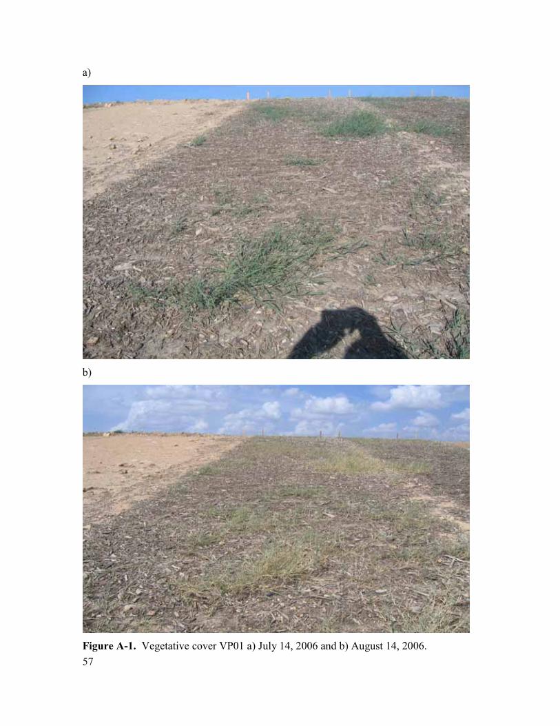
a)

b)

Figure A-1. Vegetative cover VP01 a) July 14, 2006 and b) August 14, 2006.57

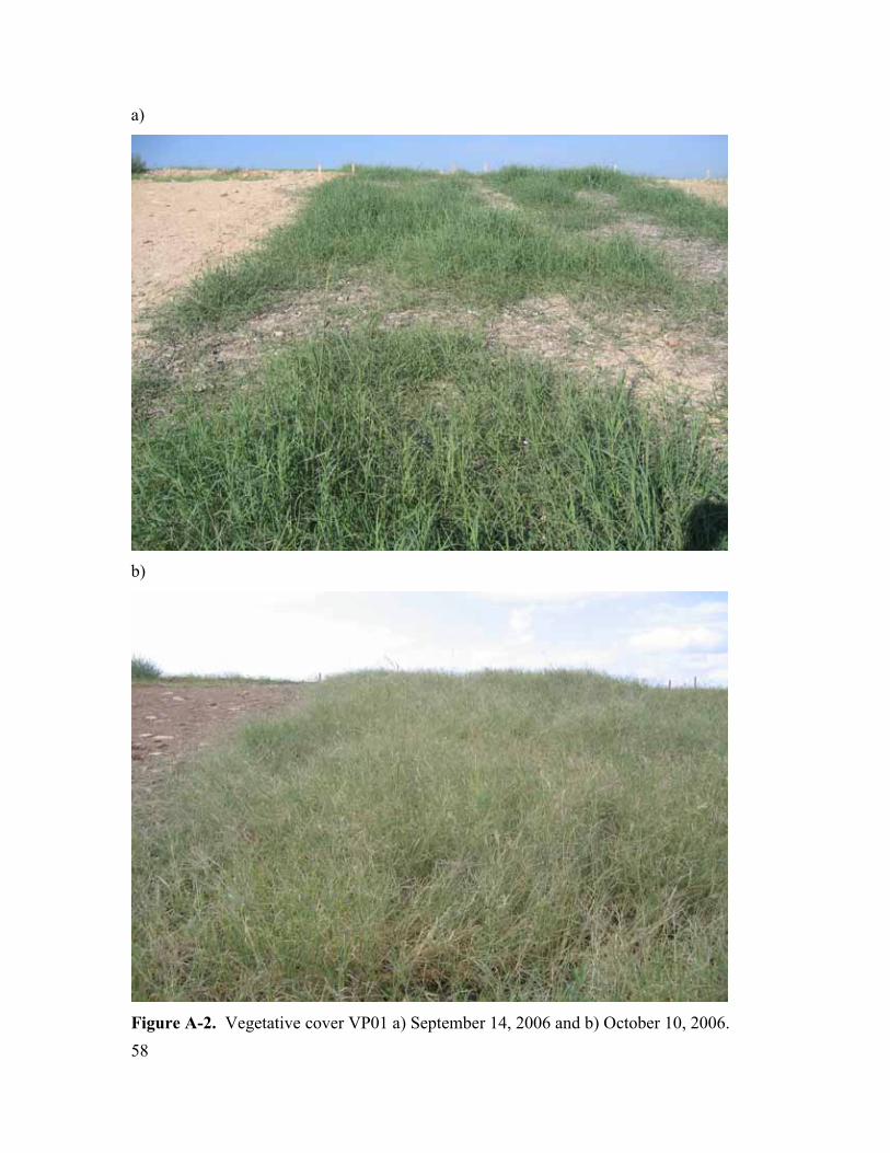
a)

b)

Figure A-2. Vegetative cover VP01 a) September 14, 2006 and b) October 10, 2006.58

a)

b)

Figure A-3. Vegetative cover VP01 a) December 14, 2006 and b) February 21, 2007.

59

a)

b)

Figure A-4. Vegetative cover VP01 a) April 19, 2007 and b) June 18, 2007.

60

a)

b)

Figure A-5. Vegetative cover VP01 a) August 20, 2007 and b) October 16, 2007.

61

a)

b)

Figure A-6. Vegetative cover VP01 a) January 3, 2008 and b) February 14, 2008.

62

Figure A-7. Vegetative cover VP01 April 17, 2008.

63

a)

b)

Figure A-8. Vegetative cover VP02 a) July 14, 2006 and b) August 14, 2006.64

a)

b)

Figure A-9. Vegetative cover VP02 a) September 14, 2006 and b) October 10, 2006.

65

a)

b)

Figure A-10. Vegetative cover VP02 a) December 14, 2006 and b) February 21, 2007.

66

a)

b)

Figure A-11. Vegetative cover VP02 a) April 19, 2007 and b) June 18, 2007.

67

a)

b)

Figure A-12. Vegetative cover VP02 a) August 20, 2007 and b) October 16, 2007.

68

a)

b)

Figure A-13. Vegetative cover VP02 a) January 3, 2008 and b) February 14, 2008.

69

Figure A-14. Vegetative cover VP02 April 17, 2008.

70

a)

b)

Figure A-15. Vegetative cover VP03 a) July 14, 2006 and b) August 14, 2006.

71

a)

b)

Figure A-16. Vegetative cover VP03 a) September 14, 2006 and b) October 10, 2006.

72

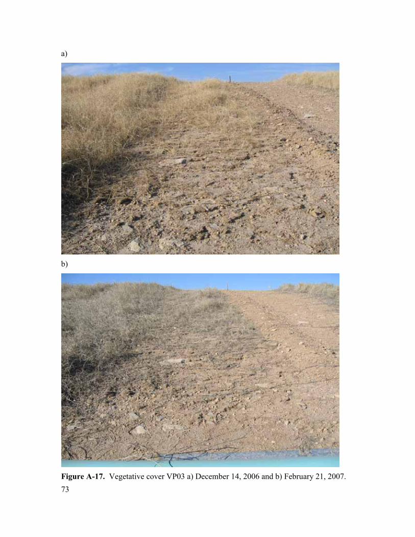
a)

b)

Figure A-17. Vegetative cover VP03 a) December 14, 2006 and b) February 21, 2007.73

a)

b)

Figure A-18. Vegetative cover VP03 a) April 19, 2007 and b) June 18, 2007.

74

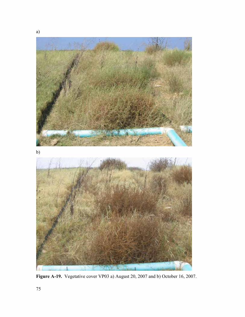
a)

b)

Figure A-19. Vegetative cover VP03 a) August 20, 2007 and b) October 16, 2007.

75

a)

b)

Figure A-20. Vegetative cover VP03 a) January 3, 2008 and b) February 14, 2008.

76

Figure A-21. Vegetative cover VP03 April 17, 2008.

77

a)

b)

Figure A-22. Vegetative cover VP04 a) July 14, 2006 and b) August 14, 2006.

78

a)

b)

Figure A-23. Vegetative cover VP04 a) September 14, 2006 and b) October 10, 2006.

79

a)

b)

Figure A-24. Vegetative cover VP04 a) December 14, 2006 and b) February 21, 2007.

80

a)

b)

Figure A-25. Vegetative cover VP04 a) April 19, 2007 and b) June 18, 2007.

81

a)

b)

Figure A-26. Vegetative cover VP04 a) August 20, 2007 and b) October 16, 2007.

82

a)

b)

Figure A-27. Vegetative cover VP04 a) January 3, 2008 and b) February 14, 2008.

83

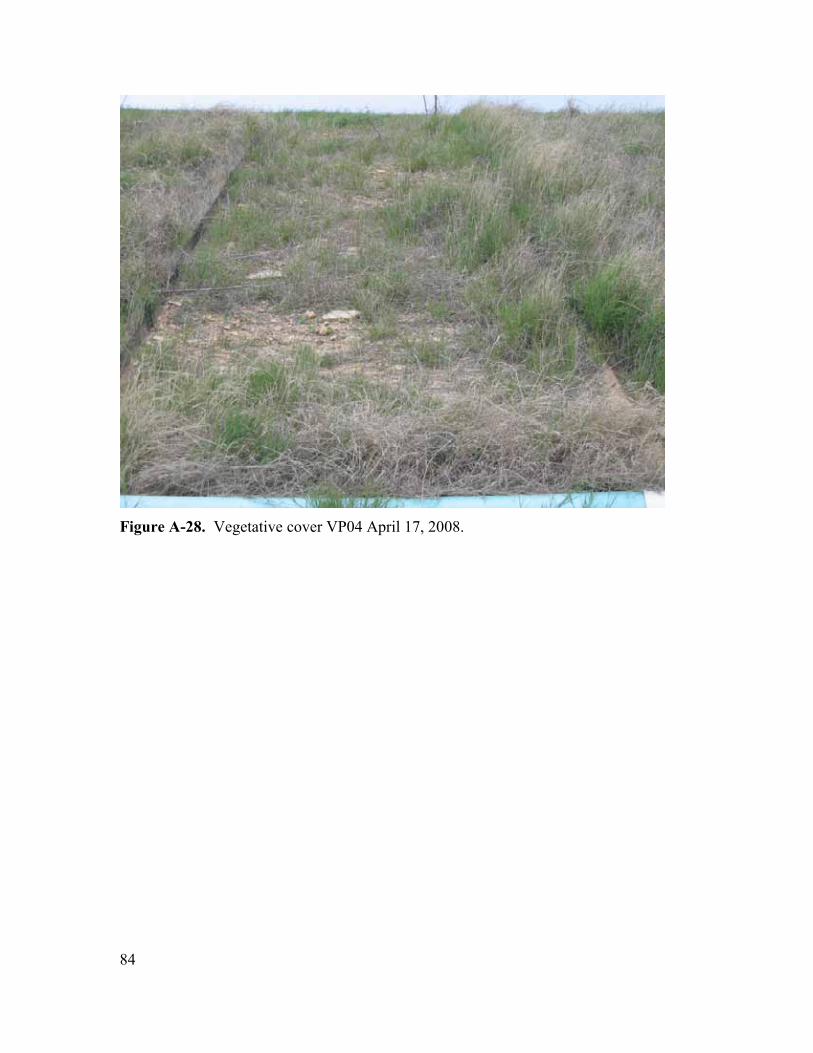
Figure A-28. Vegetative cover VP04 April 17, 2008.

84

a)

b)

Figure A-29. Vegetative cover VP05 a) July 14, 2006 and b) August 14, 2006.

85

a)

b)

Figure A-30. Vegetative cover VP05 a) September 14, 2006 and b) October 10, 2006.

86

a)

b)

Figure A-31. Vegetative cover VP05 a) December 14, 2006 and b) February 21, 20

87

a)

b)

Figure A-32. Vegetative cover VP05 a) April 19, 2007 and b) June 18, 2007.

88

a)

b)

Figure A-33. Vegetative cover VP05 a) August 20, 2007 and b) October 16, 2007.

89

a)

b)

Figure A-34. Vegetative cover VP05 a) January 3, 2008 and b) February 14, 2008.

90

Figure A-35. Vegetative cover VP05 April 17, 2008.

91

a)

b)

Figure A-36. Vegetative cover VP06 a) July 14, 2006 and b) August 14, 2006.

92

a)

b)

Figure A-37. Vegetative cover VP06 a) September 14, 2006 and b) October 10, 2006.

93

a)

b)

Figure A-38. Vegetative cover VP06 a) December 14, 2006 and b) February 21, 2007.

94

a)

b)

Figure A-39. Vegetative cover VP06 a) April 19, 2007 and b) June 18, 2007.

95

a)

b)

Figure A-40. Vegetative cover VP06 a) August 20, 2007 and b) October 16, 2007. 96

a)

b)

Figure A-41. Vegetative cover VP06 a) January 3, 2008 and b) February 14, 2008.

97

Figure A-42. Vegetative cover VP06 April 17, 2008.

98

a)

b)

Figure A-43. Vegetative cover VP07 a) July 14, 2006 and b) August 14, 2006.

99

a)

b)

Figure A-44. Vegetative cover VP07 a) September 14, 2006 and b) October 10, 2006.

100

a)

b)

Figure A-45. Vegetative cover VP07 a) December 14, 2006 and b) February 21, 2007.

101

a)

b)

Figure A-46. Vegetative cover VP07 a) April 19, 2007 and b) June 18, 2007.

102

a)

b)

Figure A-47. Vegetative cover VP07 a) August 20, 2007 and b) October 16, 2007.

103

a)

b)

Figure A-48. Vegetative cover VP07 a) January 3, 2008 and b) February 14, 2008.

104

Figure A-49. Vegetative cover VP07 April 17, 2008.

105

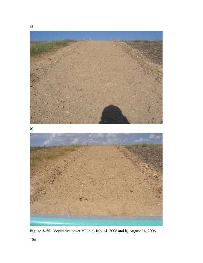
a)

b)

Figure A-50. Vegetative cover VP08 a) July 14, 2006 and b) August 14, 2006.

106

a)

b)

Figure A-51. Vegetative cover VP08 a) September 14, 2006 and b) October 10, 2006. 107

a)

b)

Figure A-52. Vegetative cover VP08 a) December 14, 2006 and b) February 21, 2007.

a) 108

b)

Figure A-53. Vegetative cover VP08 a) April 19, 2007 and b) June 18, 2007.

a)

109

b)

Figure A-54. Vegetative cover VP08 a) August 20, 2007 and b) October 16, 2007.

a)

110

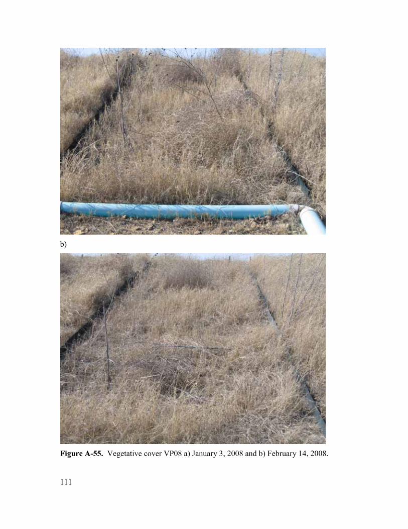
b)

Figure A-55. Vegetative cover VP08 a) January 3, 2008 and b) February 14, 2008.

111

Figure A-56. Vegetative cover VP08 April 17, 2008.

112

a)

b)

Figure A-57. Vegetative cover VP09 a) July 14, 2006 and b) August 14, 2006.

113

a)

b)

Figure A-58. Vegetative cover VP09 a) September 14, 2006 and b) October 10, 2006. 114

a)

b)

Figure A-59. Vegetative cover VP09 a) December 14, 2006 and b) February 21, 2007.

115

a)

b)

Figure A-60. Vegetative cover VP09 a) April 19, 2007 and b) June 18, 2007.

a) 116

b)

Figure A-61. Vegetative cover VP09 a) August 20, 2007 and b) October 16, 2007.

a)

117

b)

Figure A-62. Vegetative cover VP09 a) January 3, 2008 and b) February 14, 2008.

118

Figure A-63. Vegetative cover VP09 April 17, 2008.

119

a)

b)

Figure A-64. Vegetative cover VP10 a) July 14, 2006 and b) August 14, 2006.

120

a)

b)

Figure A-65. Vegetative cover VP10 a) September 14, 2006 and b) October 10, 2006.121

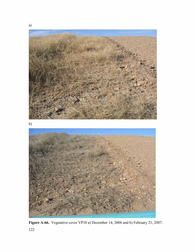
a)

b)

Figure A-66. Vegetative cover VP10 a) December 14, 2006 and b) February 21, 2007.

122

a)

b)

Figure A-67. Vegetative cover VP10 a) April 19, 2007 and b) June 18, 2007

123

a)

b)

Figure A-68. Vegetative cover VP10 a) August 20, 2007 and b) October 16, 2007.

124

a)

b)

Figure A-69. Vegetative cover VP10 a) January 3, 2008 and b) February 14, 2008.

125

Figure A-70. Vegetative cover VP10 April 17, 2008.

126

Figure A-71. Composite view of test plots VP01, VP02, VP03, VP04, and VP05

(partial view) taken December 14, 2006.

Figure A-72. Composite view of test plots VP04 (partial view), VP05, VP06, VP07,

VP08, and VP09 (partial view) taken December 14, 2006.

127

Figure A-73. Composite view of test plots VP07 (partial view), VP08, VP09, and VP10 taken December 14, 2006.

Figure A-74. Composite view of test plots VP01, VP02, VP03, VP04, and VP05 (partial view) taken April 19, 2007.

128

Figure A-75. Composite view of test plots VP04 (partial view), VP05, VP06, VP07,

VP08, and VP09 (partial view) taken April 19, 2007.

Figure A-76. Composite view of test plots VP06 (partial view), VP07, VP08, VP09, and

VP10 taken April 19, 2007

129

Figure A-77. Composite view of test plots VP01, VP02, VP03, and VP04 taken January 3, 2008.

Figure A-78. Composite view of test plots VP04 (partial view), VP05, VP06, VP07,

VP08, and VP09 (partial view) taken January 3, 2008. 130

Figure A-79. Composite view of test plots VP08, VP09, and VP10 taken January 3, 2008.

Figure A-80. Composite view of test plots VP01, VP02, VP03, VP04, and VP05 (partial view) taken April 17, 2008.

131

Figure A-81. Composite view of test plots VP04 (partial view), VP05, VP06, VP07, VP08, and VP09 (partial view) taken April 17, 2008.

Figure A-82. Composite view of test plots VP06 (partial view), VP07, VP08, VP09, and VP10 taken April 17, 2008.

132

Appendix B: Observed Runoff Volumes and Concentrations

133

Table B-1. Runoff volumes and concentrations for June 17, 2006 event one. Rainfall

(inches)

Plot Volume

(gallons)

Overflow TSS

(mg/L)

Dissolved

NO2-N +

NO3-N

(mg/L)

TKN

(mg/L)

Dissolved

PO4-P

(mg/L)

Total-

P

(mg/L)

VP01 Low OM No

VP02 High OM 5 No 1720 8.51 55.7 1.74 5.57

VP03 Hydromulch No

VP04 Untreated 23 No 20000 0.464 21.5 0.536 6.59

VP05 Low OM No

VP06 High OM No

VP07 Hydromulch 11 No 8640 0.513 8.13 1.86 5.57

VP08 Untreated 20 No 23600 0.474 25.1 0.173 7.96

VP09 Low OM No

0.36

VP10 Hydromulch No

Table B-2. Runoff volumes and concentrations for June 17, 2006 event two. Rainfall

(inches)

Plot Volume

(gallons)

Overflow TSS

(mg/L)

Dissolved

NO2-N +

NO3-N

(mg/L)

TKN

(mg/L)

Dissolved

PO4-P

(mg/L)

Total-

P

(mg/L)

VP01 Low OM 71 No 3380 4.25 26.9 1.49 7.14

VP02 High OM 95 No 5740 0.203 60.9 2.40 18.2

VP03 Hydromulch 132 No 21100 0.410 20.2 3.82 13.1

VP04 Untreated 148 Possible 20800 0.761 36.1 0.731 12.7

VP05 Low OM 78 No 5970 4.55 31.8 1.72 9.23

VP06 High OM 93 No 6170 0.108 30.6 1.95 7.68

VP07 Hydromulch 132 No 14400 0.383 17.9 2.30 10.2

VP08 Untreated 155 No 35500 0.403 27.1 0.280 8.61

VP09 Low OM 81 No 13400 2.33 28.0 1.30 8.86

1.23

VP10 Hydromulch 107 No 20000 0.260 17.8 1.09 8.29

134

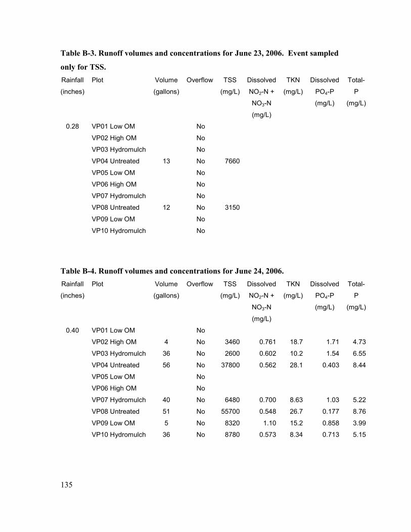
Table B-3. Runoff volumes and concentrations for June 23, 2006. Event sampled

only for TSS. Rainfall

(inches)

Plot Volume

(gallons)

Overflow TSS

(mg/L)

Dissolved

NO2-N +

NO3-N

(mg/L)

TKN

(mg/L)

Dissolved

PO4-P

(mg/L)

Total-

P

(mg/L)

VP01 Low OM No

VP02 High OM No

VP03 Hydromulch No

VP04 Untreated 13 No 7660

VP05 Low OM No

VP06 High OM No

VP07 Hydromulch No

VP08 Untreated 12 No 3150

VP09 Low OM No

0.28

VP10 Hydromulch No

Table B-4. Runoff volumes and concentrations for June 24, 2006. Rainfall

(inches)

Plot Volume

(gallons)

Overflow TSS

(mg/L)

Dissolved

NO2-N +

NO3-N

(mg/L)

TKN

(mg/L)

Dissolved

PO4-P

(mg/L)

Total-

P

(mg/L)

VP01 Low OM No

VP02 High OM 4 No 3460 0.761 18.7 1.71 4.73

VP03 Hydromulch 36 No 2600 0.602 10.2 1.54 6.55

VP04 Untreated 56 No 37800 0.562 28.1 0.403 8.44

VP05 Low OM No

VP06 High OM No

VP07 Hydromulch 40 No 6480 0.700 8.63 1.03 5.22

VP08 Untreated 51 No 55700 0.548 26.7 0.177 8.76

VP09 Low OM 5 No 8320 1.10 15.2 0.858 3.99

0.40

VP10 Hydromulch 36 No 8780 0.573 8.34 0.713 5.15

135

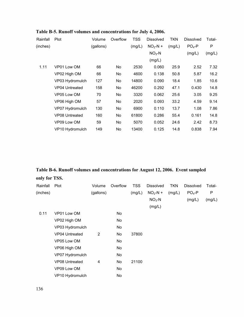
Table B-5. Runoff volumes and concentrations for July 4, 2006. Rainfall

(inches)

Plot Volume

(gallons)

Overflow TSS

(mg/L)

Dissolved

NO2-N +

NO3-N

(mg/L)

TKN

(mg/L)

Dissolved

PO4-P

(mg/L)

Total-

P

(mg/L)

VP01 Low OM 66 No 2530 0.060 25.9 2.52 7.32

VP02 High OM 66 No 4600 0.138 50.8 5.87 16.2

VP03 Hydromulch 127 No 14800 0.090 18.4 1.85 10.6

VP04 Untreated 158 No 46200 0.292 47.1 0.430 14.8

VP05 Low OM 70 No 3320 0.062 25.6 3.05 9.25

VP06 High OM 57 No 2020 0.093 33.2 4.59 9.14

VP07 Hydromulch 130 No 6900 0.110 13.7 1.08 7.86

VP08 Untreated 160 No 61800 0.286 55.4 0.161 14.8

VP09 Low OM 59 No 5070 0.052 24.6 2.42 8.73

1.11

VP10 Hydromulch 149 No 13400 0.125 14.8 0.838 7.94

Table B-6. Runoff volumes and concentrations for August 12, 2006. Event sampled

only for TSS. Rainfall

(inches)

Plot Volume

(gallons)

Overflow TSS

(mg/L)

Dissolved

NO2-N +

NO3-N

(mg/L)

TKN

(mg/L)

Dissolved

PO4-P

(mg/L)

Total-

P

(mg/L)

VP01 Low OM No

VP02 High OM No

VP03 Hydromulch No

VP04 Untreated 2 No 37800

VP05 Low OM No

VP06 High OM No

VP07 Hydromulch No

VP08 Untreated 4 No 21100

VP09 Low OM No

0.11

VP10 Hydromulch No

136

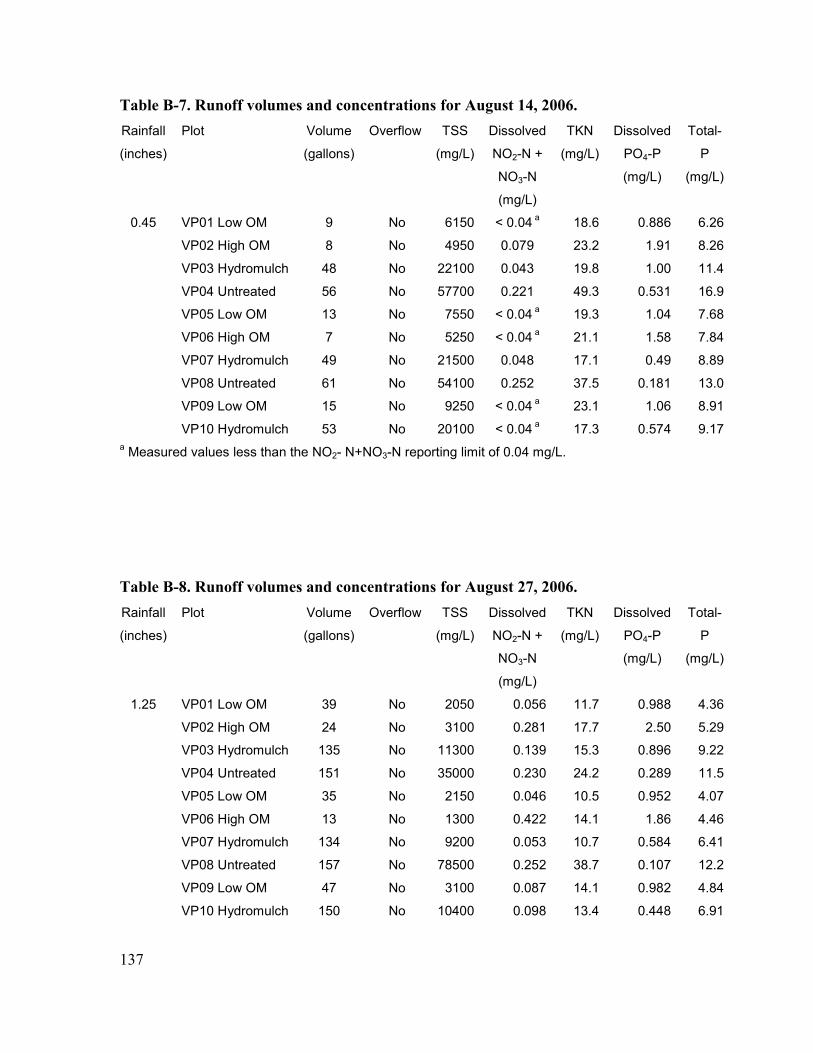
Table B-7. Runoff volumes and concentrations for August 14, 2006. Rainfall

(inches)

Plot Volume

(gallons)

Overflow TSS

(mg/L)

Dissolved

NO2-N +

NO3-N

(mg/L)

TKN

(mg/L)

Dissolved

PO4-P

(mg/L)

Total-

P

(mg/L)

VP01 Low OM 9 No 6150 < 0.04 a 18.6 0.886 6.26

VP02 High OM 8 No 4950 0.079 23.2 1.91 8.26

VP03 Hydromulch 48 No 22100 0.043 19.8 1.00 11.4

VP04 Untreated 56 No 57700 0.221 49.3 0.531 16.9

VP05 Low OM 13 No 7550 < 0.04 a 19.3 1.04 7.68

VP06 High OM 7 No 5250 < 0.04 a 21.1 1.58 7.84

VP07 Hydromulch 49 No 21500 0.048 17.1 0.49 8.89

VP08 Untreated 61 No 54100 0.252 37.5 0.181 13.0

VP09 Low OM 15 No 9250 < 0.04 a 23.1 1.06 8.91

0.45

VP10 Hydromulch 53 No 20100 < 0.04 a 17.3 0.574 9.17a Measured values less than the NO2- N+NO3-N reporting limit of 0.04 mg/L.

Table B-8. Runoff volumes and concentrations for August 27, 2006. Rainfall

(inches)

Plot Volume

(gallons)

Overflow TSS

(mg/L)

Dissolved

NO2-N +

NO3-N

(mg/L)

TKN

(mg/L)

Dissolved

PO4-P

(mg/L)

Total-

P

(mg/L)

VP01 Low OM 39 No 2050 0.056 11.7 0.988 4.36

VP02 High OM 24 No 3100 0.281 17.7 2.50 5.29

VP03 Hydromulch 135 No 11300 0.139 15.3 0.896 9.22

VP04 Untreated 151 No 35000 0.230 24.2 0.289 11.5

VP05 Low OM 35 No 2150 0.046 10.5 0.952 4.07

VP06 High OM 13 No 1300 0.422 14.1 1.86 4.46

VP07 Hydromulch 134 No 9200 0.053 10.7 0.584 6.41

VP08 Untreated 157 No 78500 0.252 38.7 0.107 12.2

VP09 Low OM 47 No 3100 0.087 14.1 0.982 4.84

1.25

VP10 Hydromulch 150 No 10400 0.098 13.4 0.448 6.91

137

Table B-9. Runoff volumes for September 3, 2006. No water quality sample

collected. Rainfall

(inches)

Plot Volume

(gallons)

Overflow TSS

(mg/L)

Dissolved

NO2-N +

NO3-N

(mg/L)

TKN

(mg/L)

Dissolved

PO4-P

(mg/L)

Total-

P

(mg/L)

VP01 Low OM 151 Yes

VP02 High OM 151 Yes

VP03 Hydromulch 150 Yes

VP04 Untreated 158 Yes

VP05 Low OM 130 No

VP06 High OM 122 No

VP07 Hydromulch 159 Yes

VP08 Untreated 157 Yes

VP09 Low OM 151 Possibly

2.68

VP10 Hydromulch 158 Yes

Table B-10. Runoff volumes and concentrations for September 17, 2006. Rainfall

(inches)

Plot Volume

(gallons)

Overflow TSS

(mg/L)

Dissolved

NO2-N +

NO3-N

(mg/L)

TKN

(mg/L)

Dissolved

PO4-P

(mg/L)

Total-

P

(mg/L)

VP01 Low OM 150 Yes 952 0.105 4.52 1.61 2.60

VP02 High OM 149 Yes 836 0.096 10.8 4.12 5.85

VP03 Hydromulch 151 Yes 17600 0.054 14.8 0.384 8.06

VP04 Untreated 157 Yes 68100 0.087 21.1 0.170 8.29

VP05 Low OM 149 Yes 1232 0.066 5.27 1.43 2.99

VP06 High OM 150 Yes 780 0.062 9.08 3.38 4.99

VP07 Hydromulch 158 Yes 18100 0.053 11.8 0.271 6.40

VP08 Untreated 157 Yes 92800 0.083 26.1 0.088 9.74

VP09 Low OM 149 Yes 2310 0.096 6.06 1.38 3.37

1.92

VP10 Hydromulch 160 Yes 23400 0.058 9.56 0.218 4.84

138

Table B-11. Runoff volumes and concentrations for October 10, 2006. No water

quality sample collected. Rainfall

(inches)

Plot Volume

(gallons)

Overflow TSS

(mg/L)

Dissolved

NO2-N +

NO3-N

(mg/L)

TKN

(mg/L)

Dissolved

PO4-P

(mg/L)

Total-

P

(mg/L)

VP01 Low OM No

VP02 High OM No

VP03 Hydromulch 27 No

VP04 Untreated 97 No

VP05 Low OM No

VP06 High OM No

VP07 Hydromulch 24 No

VP08 Untreated 102 No

VP09 Low OM No

0.45

VP10 Hydromulch 25 No

Table B-12. Runoff volumes and concentrations for October 15, 2006. Rainfall

(inches)

Plot Volume

(gallons)

Overflow TSS

(mg/L)

Dissolved

NO2-N +

NO3-N

(mg/L)

TKN

(mg/L)

Dissolved

PO4-P

(mg/L)

Total-

P

(mg/L)

VP01 Low OM 150 Yes 242 < 0.04 a 1.57 2.41 3.39

VP02 High OM 149 Yes 192 0.044 4.72 6.04 7.36

VP03 Hydromulch 151 Yes 8500 < 0.04 a 6.70 0.298 5.36

VP04 Untreated 157 Yes 19000 0.051 5.90 0.114 5.22

VP05 Low OM 149 Yes 2620 < 0.04 a 1.19 2.36 3.48

VP06 High OM 150 Yes 102 < 0.04 a 4.29 5.07 5.86

VP07 Hydromulch 158 Yes 7000 <0.04 a 7.43 0.195 4.41

VP08 Untreated 157 Yes 24100 0.045 8.30 0.050 5.23

VP09 Low OM 149 Yes 416 0.050 2.07 2.41 2.78

2.51

VP10 Hydromulch 160 Yes 9020 < 0.04 a 4.59 0.186 3.62a Measured values less than the NO2-N+NO3-N reporting limit of 0.04 mg/L.

139

Table B-13. Runoff volumes for October 24, 2006. No water quality sample

collected. Rainfall

(inches)

Plot Volume

(gallons)

Overflow TSS

(mg/L)

Dissolved

NO2-N +

NO3-N

(mg/L)

TKN

(mg/L)

Dissolved

PO4-P

(mg/L)

Total-

P

(mg/L)

VP01 Low OM No

VP02 High OM No

VP03 Hydromulch 9 No

VP04 Untreated 7 No

VP05 Low OM No

VP06 High OM No

VP07 Hydromulch 7 No

VP08 Untreated 6 No

VP09 Low OM No

0.26

VP10 Hydromulch 7 No

Table B-14. Runoff volumes and concentrations for November 5, 2006. Rainfall

(inches)

Plot Volume

(gallons)

Overflow TSS

(mg/L)

Dissolved

NO2-N +

NO3-N

(mg/L)

TKN

(mg/L)

Dissolved

PO4-P

(mg/L)

Total-

P

(mg/L)

VP01 Low OM 150 Yes 300 0.122 5.01 2.53 3.08

VP02 High OM 151 Yes 304 0.126 9.16 6.06 7.01

VP03 Hydromulch 151 Yes 17900 0.165 16.1 0.288 7.89

VP04 Untreated 160 Yes 25500 0.179 20.0 0.100 7.29

VP05 Low OM 150 Yes 284 0.121 4.15 2.63 3.43

VP06 High OM 150 Yes 174 0.111 5.76 4.75 5.95

VP07 Hydromulch 158 Yes 16300 0.160 11.9 0.195 6.91

VP08 Untreated 156 Yes 42400 0.173 25.0 0.038 8.81

VP09 Low OM 150 Yes 366 0.464 4.81 2.75 4.00

2.56

VP10 Hydromulch 159 Yes 16200 0.178 14.1 0.162 6.06

140

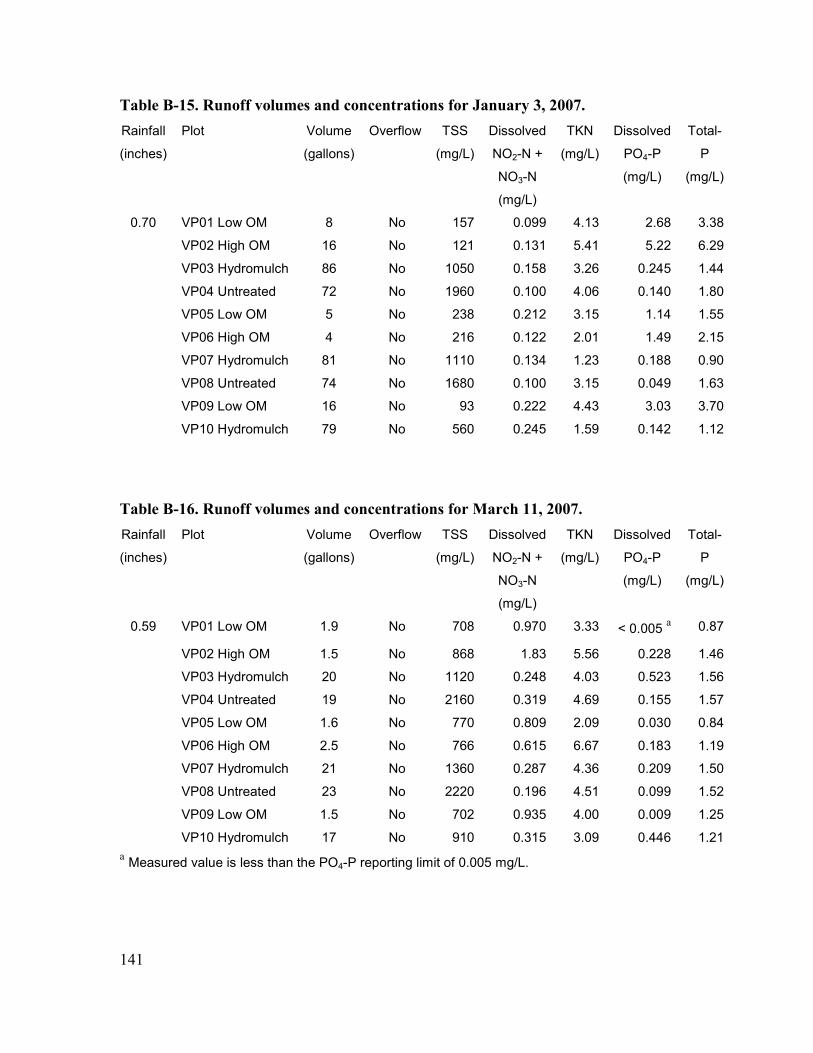
Table B-15. Runoff volumes and concentrations for January 3, 2007. Rainfall

(inches)

Plot Volume

(gallons)

Overflow TSS

(mg/L)

Dissolved

NO2-N +

NO3-N

(mg/L)

TKN

(mg/L)

Dissolved

PO4-P

(mg/L)

Total-

P

(mg/L)

VP01 Low OM 8 No 157 0.099 4.13 2.68 3.38

VP02 High OM 16 No 121 0.131 5.41 5.22 6.29

VP03 Hydromulch 86 No 1050 0.158 3.26 0.245 1.44

VP04 Untreated 72 No 1960 0.100 4.06 0.140 1.80

VP05 Low OM 5 No 238 0.212 3.15 1.14 1.55

VP06 High OM 4 No 216 0.122 2.01 1.49 2.15

VP07 Hydromulch 81 No 1110 0.134 1.23 0.188 0.90

VP08 Untreated 74 No 1680 0.100 3.15 0.049 1.63

VP09 Low OM 16 No 93 0.222 4.43 3.03 3.70

0.70

VP10 Hydromulch 79 No 560 0.245 1.59 0.142 1.12

Table B-16. Runoff volumes and concentrations for March 11, 2007. Rainfall

(inches)

Plot Volume

(gallons)

Overflow TSS

(mg/L)

Dissolved

NO2-N +

NO3-N

(mg/L)

TKN

(mg/L)

Dissolved

PO4-P

(mg/L)

Total-

P

(mg/L)

VP01 Low OM 1.9 No 708 0.970 3.33 < 0.005 a 0.87

VP02 High OM 1.5 No 868 1.83 5.56 0.228 1.46

VP03 Hydromulch 20 No 1120 0.248 4.03 0.523 1.56

VP04 Untreated 19 No 2160 0.319 4.69 0.155 1.57

VP05 Low OM 1.6 No 770 0.809 2.09 0.030 0.84

VP06 High OM 2.5 No 766 0.615 6.67 0.183 1.19

VP07 Hydromulch 21 No 1360 0.287 4.36 0.209 1.50

VP08 Untreated 23 No 2220 0.196 4.51 0.099 1.52

VP09 Low OM 1.5 No 702 0.935 4.00 0.009 1.25

0.59

VP10 Hydromulch 17 No 910 0.315 3.09 0.446 1.21a Measured value is less than the PO4-P reporting limit of 0.005 mg/L.

141

Table B-17. Runoff volumes and concentrations for April 30, 2007. Rainfall

(inches)

Plot Volume

(gallons)

Overflow TSS

(mg/L)

Dissolved

NO2-N +

NO3-N

(mg/L)

TKN

(mg/L)

Dissolved

PO4-P

(mg/L)

Total-

P

(mg/L)

VP01 Low OM 4 No 396 0.310 2.71 0.442 1.09

VP02 High OM 3 No 324 0.449 4.80 1.57 2.33

VP03 Hydromulch 75 No 4340 0.254 4.59 0.135 2.56

VP04 Untreated 74 No 8520 0.257 6.45 0.036 2.80

VP05 Low OM 12 No 1600 0.299 4.33 0.557 1.75

VP06 High OM 4 No 320 0.323 2.85 0.778 1.31

VP07 Hydromulch 71 No 3020 0.243 3.27 0.076 1.59

VP08 Untreated 91 No 8000 0.293 6.26 0.017 2.57

VP09 Low OM 5 No 368 0.313 4.30 0.623 1.16

0.97

VP10 Hydromulch 55 No 2640 0.215 5.00 0.061 1.78

Table B-18. Runoff volumes and concentrations for June 1, 2007. Rainfall

(inches)

Plot Volume

(gallons)

Overflow TSS

(mg/L)

Dissolved

NO2-N +

NO3-N

(mg/L)

TKN

(mg/L)

Dissolved

PO4-P

(mg/L)

Total-

P

(mg/L)

VP01 Low OM 1.6 No 211 0.480 2.08 0.246 0.63

VP02 High OM 1.9 No 242 0.847 1.99 0.736 1.12

VP03 Hydromulch 67 No 1800 0.327 3.38 0.197 1.62

VP04 Untreated 74 No 7350 0.433 7.49 0.044 3.12

VP05 Low OM 3.5 No 352 0.428 2.35 0.356 0.97

VP06 High OM 2.1 No 193 0.364 1.23 0.386 0.73

VP07 Hydromulch 61 No 980 0.349 3.27 0.133 1.42

VP08 Untreated 78 No 9650 0.481 8.54 0.032 3.27

VP09 Low OM 1.6 No 161 0.445 2.46 0.527 0.90

0.76

VP10 Hydromulch 50 No 1140 0.361 3.04 0.090 1.13

142 Table B-19. Runoff volumes and concentrations for October 22, 2007.

Rainfall

(inches)

Plot Volume

(gallons)

Overflow TSS

(mg/L)

Dissolved

NO2-N +

NO3-N

(mg/L)

TKN

(mg/L)

Dissolved

PO4-P

(mg/L)

Total-

P

(mg/L)

VP01 Low OM 1.6 No 150 0.577 6.54 1.64 1.90

VP02 High OM 1.5 No 215 1.24 4.46 2.44 2.83

VP03 Hydromulch 1.8 No 173 2.06 3.70 0.214 0.47

VP04 Untreated 17 No 135 0.360 14.8 0.460 0.82

VP05 Low OM 1.7 No 152 0.710 3.82 0.813 1.04

VP06 High OM 1.9 No 248 0.916 2.30 0.819 1.14

VP07 Hydromulch 3.1 No 178 1.31 3.41 0.291 0.53

VP08 Untreated 9 No 116 0.395 2.87 0.109 0.31

VP09 Low OM 2.1 No 193 2.61 55.4 7.12 8.72

0.65

VP10 Hydromulch 1.1 No 351 2.64 63.0 2.16 3.59

Table B-20. Runoff volumes and concentrations for November 24, 2007. Rainfall

(inches)

Plot Volume

(gallons)

Overflow TSS

(mg/L)

Dissolved

NO2-N +

NO3-N

(mg/L)

TKN

(mg/L)

Dissolved

PO4-P

(mg/L)

Total-

P

(mg/L)

VP01 Low OM 7 No 199 0.608 6.36 1.54 2.12

VP02 High OM 9 No 185 0.800 29.0 2.57 3.30

VP03 Hydromulch 76 No 62 0.214 1.15 0.268 0.50

VP04 Untreated 154 No 144 0.092 0.90 0.095 0.42

VP05 Low OM 10 No 125 1.86 4.37 0.729 1.08

VP06 High OM 8 No 28 1.02 5.34 1.26 1.82

VP07 Hydromulch 44 No 57 0.420 1.59 0.267 0.51

VP08 Untreated 115 No 105 0.101 1.01 0.045 0.35

VP09 Low OM 10 No 86 0.975 8.20 2.14 2.68

1.78

VP10 Hydromulch 16a No 90 0.575 2.78 0.342 0.60a Possible berm breach to outside of plot (breach did not affect nearby plot VP09).

Table B-21. Runoff volumes and concentrations for February 18, 2008. 143

Rainfall

(inches)

Plot Volume

(gallons)

Overflow TSS

(mg/L)

Dissolved

NO2-N +

NO3-N

(mg/L)

TKN

(mg/L)

Dissolved

PO4-P

(mg/L)

Total-

P

(mg/L)

VP01 Low OM 7 No 492 1.44 9.56 1.15 2.32

VP02 High OM 16 No 404 1.68 4.79 2.80 3.97

VP03 Hydromulch 87 No 672 0.469 3.78 0.273 1.16

VP04 Untreated 126 No 1900 0.255 4.31 0.115 1.80

VP05 Low OM 12 No 608 2.78 5.75 1.14 2.16

VP06 High OM 13 No 576 1.88 7.46 2.22 2.55

VP07 Hydromulch 92 No 452 0.511 3.69 0.313 1.02

VP08 Untreated 125 No 972 3.20 113 1.30 5.68

VP09 Low OM 9 No 708 0.382 5.76 0.117 1.14

1.10

VP10 Hydromulch 70 No 690 0.423 7.52 0.257 1.78

Table B-22. Runoff volumes and concentrations for March 16, 2008. Rainfall

(inches)

Plot Volume

(gallons)

Overflow TSS

(mg/L)

Dissolved

NO2-N +

NO3-N

(mg/L)

TKN

(mg/L)

Dissolved

PO4-P

(mg/L)

Total-

P

(mg/L)

VP01 Low OM 6 No 132 0.208 3.41 1.24 1.67

VP02 High OM 19 No 106 0.291 3.96 3.46 3.88

VP03 Hydromulch 133 No 155 0.101 2.05 0.152 0.36

VP04 Untreated 142 No 536 0.121 1.97 0.048 0.60

VP05 Low OM 13 No 282 0.389 2.62 1.47 1.92

VP06 High OM 8 No 140 0.432 3.75 2.28 2.76

VP07 Hydromulch 107 No 82 0.113 2.26 0.187 0.37

VP08 Untreated 145 No 184 0.140 1.59 0.022 0.30

VP09 Low OM 7 No 137 0.493 4.33 1.62 2.46

1.37

VP10 Hydromulch 104 No 232 0.073 3.33 0.166 0.54

Table B-23. Runoff volumes and concentrations for April 9, 2008.

144

Rainfall

(inches)

Plot Volume

(gallons)

Overflow TSS

(mg/L)

Dissolved

NO2-N +

NO3-N

(mg/L)

TKN

(mg/L)

Dissolved

PO4-P

(mg/L)

Total-

P

(mg/L)

VP01 Low OM 12 No 109 0.855 5.38 1.20 1.75

VP02 High OM 24 No 113 0.620 5.05 2.91 3.53

VP03 Hydromulch 146 No 200 0.280 2.49 0.080 0.47

VP04 Untreated 157 No 950 0.265 2.90 0.032 1.00

VP05 Low OM 12 No 202 1.39 3.48 1.10 1.66

VP06 High OM 14 No 143 0.977 5.36 2.54 3.22

VP07 Hydromulch 120 No 114 0.213 2.31 0.093 0.41

VP08 Untreated 158 No 220 0.274 2.33 0.018 0.44

VP09 Low OM 10 No 135 1.77 8.22 1.36 2.54

0.87

VP10 Hydromulch 101 No 404 0.188 3.13 0.054 0.71

145

Appendix C – Monthly and Bimonthly Narrative Observations

146

The following are narrative observations recorded monthly from July 14, 2006 through

October 13, 2006, and then bimonthly thereafter, due to the attainment of 70 percent

vegetative cover on the compost plots. Pictorial observations are presented in Appendix

A. Of note, due to technical difficulties, pictorial observations associated with the

October 13, 2006 written observations were taken on October 10, 2006 in association

with a small storm event that had volume measured but was not sampled.

July 14, 2006 - Monthly Narrative Observations

All compost test plots have a good distribution of vegetation from top to bottom of each

plot. Vegetation is greener and appears to be healthier than vegetation growing on the

hydromulch plots. All compost plots continue to have new emergence of vegetation.

Test plots VP01, VP06, and VP09 (all low or high OM compost plots) have some runner

development in areas where vegetation is more mature. Due to the uniformity of the

plots, water runoff occurs in sheet form. No rill development has occurred on any

compost plots with the exception of VP09 (a “wash” area resulting from focused

supplemental watering was noted near the center of that plot). For all compost test plots,

the compost blend is still present and no areas of bare ground were observed.

The hydromulch plots have more vegetative coverage than the rest of the test plots with

the exception of VP03 (10 percent coverage; see July 14, 2006 - Table 4-4). Vegetative

coverage is limited to the upper two-thirds of each plot. Vegetation is more mature and

runner development is more advanced in the hydromulch plots than the compost test

plots. Vegetation in the hydromulch plots is not as green and lush as vegetation growing

in the compost plots and is beginning to “grey” in color due to stress from extreme

drought conditions. Also, leaves are thinning due to drought conditions. Hydromulch

fibers are still present in each plot. However, bare ground is visible in all plots,

especially in the lower half of each plot. Erosion is occurring in sheet form with a very

small amount of rill development in each hydromulch plot.

147

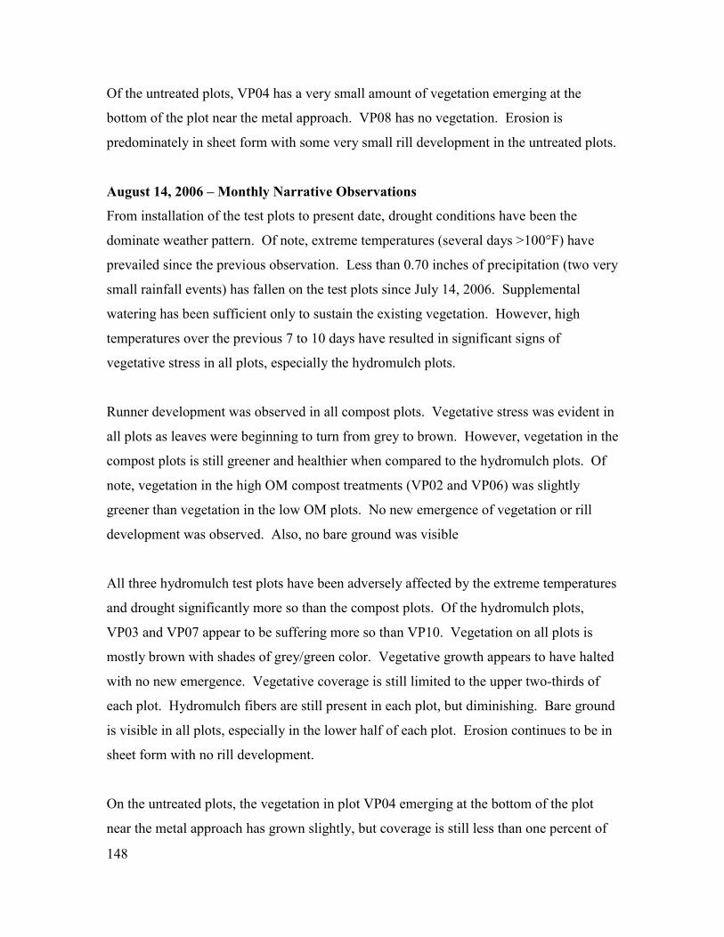
Of the untreated plots, VP04 has a very small amount of vegetation emerging at the

bottom of the plot near the metal approach. VP08 has no vegetation. Erosion is

predominately in sheet form with some very small rill development in the untreated plots.

August 14, 2006 – Monthly Narrative Observations

From installation of the test plots to present date, drought conditions have been the

dominate weather pattern. Of note, extreme temperatures (several days >100°F) have

prevailed since the previous observation. Less than 0.70 inches of precipitation (two very

small rainfall events) has fallen on the test plots since July 14, 2006. Supplemental

watering has been sufficient only to sustain the existing vegetation. However, high

temperatures over the previous 7 to 10 days have resulted in significant signs of

vegetative stress in all plots, especially the hydromulch plots.

Runner development was observed in all compost plots. Vegetative stress was evident in

all plots as leaves were beginning to turn from grey to brown. However, vegetation in the

compost plots is still greener and healthier when compared to the hydromulch plots. Of

note, vegetation in the high OM compost treatments (VP02 and VP06) was slightly

greener than vegetation in the low OM plots. No new emergence of vegetation or rill

development was observed. Also, no bare ground was visible

All three hydromulch test plots have been adversely affected by the extreme temperatures

and drought significantly more so than the compost plots. Of the hydromulch plots,

VP03 and VP07 appear to be suffering more so than VP10. Vegetation on all plots is

mostly brown with shades of grey/green color. Vegetative growth appears to have halted

with no new emergence. Vegetative coverage is still limited to the upper two-thirds of

each plot. Hydromulch fibers are still present in each plot, but diminishing. Bare ground

is visible in all plots, especially in the lower half of each plot. Erosion continues to be in

sheet form with no rill development.

On the untreated plots, the vegetation in plot VP04 emerging at the bottom of the plot

near the metal approach has grown slightly, but coverage is still less than one percent of

148

the total plot. VP08 has no vegetation. Erosion continues to be in sheet form with some

very small rill development, especially in VP08.

September 14, 2006 – Monthly Narrative Observations

Cooler temperatures (< 100°F) and significant rainfall (3.93 inches) have occurred over

the past few weeks. These weather conditions have allowed for a significant increase in

vegetative coverage in all compost plots (Table 4-4). Some increase in vegetative

coverage was noted for the hydromulch plots as well.

Vegetative health for the compost plots is significantly better than previous visits as

evident in the deep green vegetative color and large leaf development. Vegetation in the

compost plots is greener and healthier than that of the hydromulch plots. Runner

development has significantly improved since the last visit and is spreading to nearby

plots. No distinctions can be made between the low and high organic matter compost

plots with the exception of percent vegetative coverage (low OM slightly higher; Table 4-

4). Erosion continues to be in sheet form with no rill development. The compost blend is

still present in all plots and no bare spots were observed.

While vegetation in the hydromulch plots has rebounded due to recent favorable weather

conditions, the effects have been less significant than those experienced in the compost

plots. Vegetation is greener than the previous visit, but still has a slight tint of grey color.

Growth is apparent with some runner and leaf advancement in all hydromulch plots.

However, when compared to the compost plots, runners and leaves are thinner and less

abundant in the hydromuch plots. All hydromulch plots are experiencing vegetation

encroachment from nearby compost plots, especially VP10. Hydromulch fibers are still

present in each plot, but continue to recede. Bare ground is visible in all plots, especially

in the lower half of each plot. Minimal rill development was observed in each

hydromulch plot as erosion is mainly in sheet form.

149

No significant vegetative changes have occurred at the untreated plots since the previous

visit. Very slight rill development was observed at VP08. Sheet erosion continues to

dominate both untreated plots.

October 13, 2006 – Monthly Narrative Observations

Additional rainfall has permitted vegetation in the compost plots to continue to grow and

spread considerably. Total rainfall amounts, since the September observations, were

noted to be 2.37 inches. These timely rainfall events have also yielded increases of

vegetative coverage in the hydromulch plots (Table 4-4). However, most of this increase

in coverage in the hydromulch plots is attributed to runner encroachment from nearby

compost plots.

The vegetative health of the compost plots is good, but signs of stress (brown spots on

leaves) are evident in all compost plots. Compared to the hydromulch plots, vegetation in

the compost plots continues to be greener and healthier. Significant development of

vegetative runners was apparent. Also, the runners from the compost plots continue to

spread to nearby plots. VP05 has a small bare spot near the bottom of the plot. Dense

vegetative coverage prohibits visual inspection of the ground beneath. The project

requirement of the compost plots attaining 70 percent coverage was met in October 2006,

thus, leading to bimonthly vegetative monitoring thereafter.

Vegetation on the hydromulch plots is green and growing, but less vigorously than on the

compost plots. Of note, VP07 is somewhat browner than the other hydromulch plots.

Vegetative encroachment from nearby compost plots continues to occur in all

hydromulch plots, especially in VP10. Hydromulch fibers are still present in each

hydromulch plot, but continue to dwindle. Erosion continues to occur predominately in

sheet form with very slight development of existing rills observed in VP07 and VP10.

The untreated plots are experiencing runner encroachment from nearby compost plots.

No new emergence was observed. Without runner encroachment from VP09, VP08

150

would be bare. Sheet erosion continues to dominate both plots with minimal rill

development was observed in VP08.

December 14, 2006 – Bimonthly Narrative Observations

A significant amount of precipitation (5.93 inches) has occurred since the October 13,

2006 observations. Vegetation in the compost plots has continued to grow and spread

(Table 4-4). Vegetative coverage increases, mainly from runner encroachment, were

observed in the hydromulch plots as well.

Vegetation is now dormant with complete coverage in all compost plots. Compared to

the hydromulch plots, vegetation in the compost plots is denser and taller. Vegetation has

continued to spread from the compost plots to adjoining plots. No visual distinctions

could be made in the amounts of vegetative cover between the low and high organic

matter compost treatments. Dense vegetative growth prohibited visual inspection of

erosion; however, “spot checks”, performed by moving the vegetation aside by hand,

revealed no apparent soil erosion in any compost plot. In fact, the compost treatment was

observed to be in place and no bare ground was visible.

Vegetation in the hydromulch plots is also dormant. While a slight increase in vegetative

coverage was noted, the majority of the coverage increase is due to encroachment from

nearby compost plots. Hydromulch fibers continue to recede and exist only in scattered

patches. A significant amount of visible erosion has occurred since the previous

observations were performed. Erosion continues to be in sheet form with scouring

occurring below each scattered hydromulch patch (see photograph below taken 12/14/06)

with some slightly advanced rill development in VP07 and VP10.

The untreated plots have encountered a slight increase in coverage due to vegetative

encroachment from nearby compost plots. Of note, newly emerged vegetation (possibly

weeds) was observed in both plots, but noted to be scarce. Both plots have experienced

significant erosion since the previous observations. Existing rill development has

advanced slightly in VP08. Sheet erosion continues to dominate both untreated plots.

151

Close-up View of Scouring Occurring near the Bottom of VP07

February 21, 2007 – Bimonthly Narrative Observations

Rainfall totaling 4.01 inches has occurred at the test plots since the December 14, 2006

observations were conducted. Vegetation in all plots is dormant. No change was

observed at the compost plots since the December 2006 observations.

No vegetative changes were noted for the hydromulch test plots. Erosion continues to be

in sheet form with a slight increase in scouring occurring in VP07 and VP10 since the last

visit.

No vegetative change for the untreated plots has occurred since the previous observations

were conducted. Rill development has advanced slightly in VP08. Erosion continues to

occur predominately in sheet form.

152

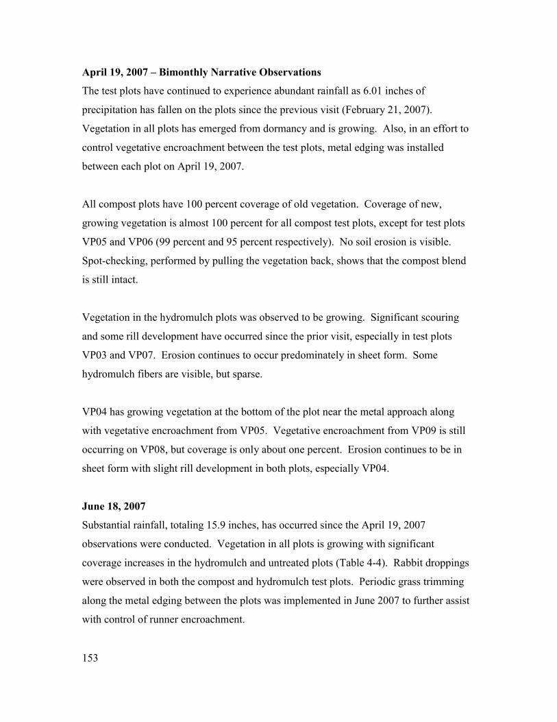
April 19, 2007 – Bimonthly Narrative Observations

The test plots have continued to experience abundant rainfall as 6.01 inches of

precipitation has fallen on the plots since the previous visit (February 21, 2007).

Vegetation in all plots has emerged from dormancy and is growing. Also, in an effort to

control vegetative encroachment between the test plots, metal edging was installed

between each plot on April 19, 2007.

All compost plots have 100 percent coverage of old vegetation. Coverage of new,

growing vegetation is almost 100 percent for all compost test plots, except for test plots

VP05 and VP06 (99 percent and 95 percent respectively). No soil erosion is visible.

Spot-checking, performed by pulling the vegetation back, shows that the compost blend

is still intact.

Vegetation in the hydromulch plots was observed to be growing. Significant scouring

and some rill development have occurred since the prior visit, especially in test plots

VP03 and VP07. Erosion continues to occur predominately in sheet form. Some

hydromulch fibers are visible, but sparse.

VP04 has growing vegetation at the bottom of the plot near the metal approach along

with vegetative encroachment from VP05. Vegetative encroachment from VP09 is still

occurring on VP08, but coverage is only about one percent. Erosion continues to be in

sheet form with slight rill development in both plots, especially VP04.

June 18, 2007

Substantial rainfall, totaling 15.9 inches, has occurred since the April 19, 2007

observations were conducted. Vegetation in all plots is growing with significant

coverage increases in the hydromulch and untreated plots (Table 4-4). Rabbit droppings

were observed in both the compost and hydromulch test plots. Periodic grass trimming

along the metal edging between the plots was implemented in June 2007 to further assist

with control of runner encroachment.

153

Coverage of new, growing vegetation is almost 100 percent on all compost test plots.

VP05 and VP06 have a few bare spots. A few weeds were observed in all compost plots.

Because of the dense vegetation, visual observation of soil erosion was difficult. Spot

checks revealed that erosion continues to occur in sheet form with no rill development.

The compost treatment is still present as random spot checks were conducted in all

compost plots by digging (by hand) through the compost-blend until the soil beneath was

visible.

A notable increase in vegetative coverage was observed in all hydromulch plots since the

previous bimonthly observations. A few weeds were observed in all hydromulch plots.

Increased vegetative cover made erosion observations difficult; however, spot checks

revealed erosion is still predominantly in sheet form with scouring occurring only below

the remaining hydromulch fibers. No major advancement of the few existing rills was

noted. Some hydromulch fibers are visible, but sparse.

A notable increase in vegetative coverage was observed in both bare plots since the

previous observations were performed. Sheet erosion continues to dominate both plots.

August 20, 2007

Rainfall has been abundant since the June 18, 2007 visit as 7.44 inches was recorded at

the test plots. Vegetation in all plots is growing with notable coverage increases in the

untreated plots (Table 4-4). Vegetative stress (brown leaves) is apparent in all plots due

to recent high temperatures (a few days >100 °F). Periodic grass trimming along the

metal edging continues to occur in an effort to control runner encroachment between

plots.

All compost plots have complete vegetative coverage. Compost plot vegetation was

noted to be denser than the hydromulch and untreated plots. A few weeds were observed

in all compost plots; however, fewer tumbleweeds (if any) were observed in the compost

plots than the hydromulch or untreated plots. Visual observation of soil erosion was not

possible due to the dense vegetation in the compost plots. Spot checks revealed erosion

154

is occurring in sheet form with no rill development. Random checks conducted in each

compost plot revealed the compost-blend to be intact with a notable increase in

vegetative root growth.

Vegetative coverage for all hydromulch plots is now 100 percent. In comparison to the

compost plots, the hydromulch plots have more weeds (especially tumbleweed). Similar

to the compost plots; visual observation of soil erosion was not possible. Spot checks

performed in each hydromulch plot revealed some soil erosion in sheet form with

scouring occurring below the remaining hydromulch fibers. The hydromulch fibers

continue to erode.

A significant increase in vegetative coverage, due to abundant rainfall, was observed in

both untreated plots (especially VP08). However, vegetation density was observed to be

notably less than the compost or hydromulch plots. Erosion continues to occur in sheet

form with no rill development.

October 16, 2007

A total of 4.25 inches of rainfall was measured at the plots since the August 20, 2007

visit. Most of the rainfall occurred in the first half of September 2007. Vegetation in all

plots is growing. However, an increase in vegetative stress (brown/yellow leaves), due to

recent dry conditions, was observed in all plots. The untreated plots continue to

experience noteworthy coverage increases (Table 4-4). Grass trimming along the metal

edging continues to occur in an effort to control runner encroachment between the plots.

Of note, wildlife presence was apparent as several of the collection tanks contained mice,

and a few contained frogs. One collection tank had a small snake in it. All wildlife was

removed from the tanks.

All compost plots have complete vegetative coverage. Vegetation continues to be denser

in the compost plots than the hydromulch or untreated plots. While a few weeds exist in

each compost plot, all compost plots were observed to be less impacted by weeds than the

hydromulch or bare plots. Visual observation of soil erosion was not possible due to the

155

dense vegetative cover. Spot checks revealed no rill development, so erosion is occurring

as sheet form. Random checks also revealed the compost treatment to be intact and an

increase in vegetative root growth. Of note, mice nests were discovered in plot VP06.

Vegetative coverage for all hydromulch plots is complete and denser than the previous

visit. However, the vegetation in the hydromulch plots remains less dense with more

weeds when compared to the compost plots. Dense vegetation prohibited visual

observation of soil erosion for all hydromulch plots. Spot checks revealed for signs of

erosion indicated some scouring below the remaining hydromulch fibers.

Vegetative coverage for both untreated plots is at or near 100 percent. The vegetation in

VP08 is denser than VP04. However, vegetative density continues to be considerably

less than the compost or hydromulch plots. No rill development was observed. Erosion

continues to occur in sheet form.

Due to logistical constraints, no bimonthly observations were recorded in December

2007, but instead bimonthly observations were recorded on January 3, 2008.

January 3, 2008

A total of 3.18 inches of rainfall has occurred at the plots since the October 16, 2007

visit. Vegetation in all plots is dormant. Vegetative coverage did not change from the

previous visit (Table 4-4). Evidence of wildlife continues to be observed. Several of the

collection tanks contained mice, which were removed. Mice nests, as in October 2007,

were observed in test plot VP06.

All compost plots have complete vegetative coverage. Dense vegetation prevails for all

compost plots. The compost-blend is still intact and vegetative root development is

denser and more advanced than the previous visit. Dense vegetation prevented visual

observation of soil erosion. Spot checks revealed erosion continues to occur in sheet

form with no rill development.

156

No vegetative changes have occurred on the hydromulch plots since the previous visit.

Of the hydromulch plots, VP07 and VP10 are denser in vegetative cover than VP03.

Thick vegetative cover prohibited visual observation of soil erosion for all hydromulch

plots. Spot checks revealed that soil erosion is primarily in sheet form with some

scouring occurring only below the remaining hydromulch fibers, especially VP03.

Little change from the previous visit was noted for the untreated plots. VP04 is

approaching 100 percent coverage, while VP08 has obtained complete coverage (Table 4-

4). Vegetative density continues to be less than the compost or hydromulch plots. No rill

development was observed. Erosion continues to occur in sheet form. More rocks were

visible than the previous visit.

February 14, 2008

Only 0.26 inches of rainfall has occurred at the plots since the January 3, 2008 visit. The

vegetation in all test plots is still dormant. No change in vegetative coverage or soil

erosion was observed in any test plot. Evidence of wildlife was indicated. Dead mice

were found in several of the tanks and removed. Mice nest were observed within several

plots associated with the compost and hydromulch treatments.

April 17, 2008

Abundant rainfall totaling 7.59 inches has occurred at the plots since the February 14,

2008 visit. New vegetation is emerging in all test plots. No change in vegetative

coverage from the previous visit was noted for all test plots. Evidence of wildlife was

abundant in the compost and hydromulch plots.

New vegetation is visible in all compost plots. The compost plots continue to have

denser vegetation than the hydromulch or untreated plots. The compost-blend remains

intact. Observation of soil erosion was prevented by dense vegetation. Spot checks

revealed erosion continues to occur in sheet form with no rill development. Of note,

extensive mouse tunnels in the compost-blend were observed throughout all compost

plots. Mice and nests were observed in each compost plot.

157

All hydromulch plots have complete vegetation coverage with new vegetation emerging.

VP10 continues to have the denser vegetative cover than the other hydromulch plots.

While the hydromulch plots are denser in vegetative cover than the untreated plots, they

remain less dense than the compost plots. Erosion observations were not possible due to

the dense vegetative cover. Spot checks revealed erosion continues to occur in sheet

form. A few mice nests were observed in each hydromulch plot.

The only untreated plot to not have complete vegetative coverage is VP04 (95 percent).

The vegetation in VP08 continues to be denser than VP04. Regarding overall vegetation

density, the untreated plots remain the least dense compared to the compost or

hydromulch plots. No rill development was observed. Erosion continues to occur in

sheet form. More rocks were visible than the previous visit.

158

Appendix C: Statistical Details

159

Low OM Treatment > ## LOW OM > ## > summary(LowOM.mr) Call: lm(formula = Runoff_in ~ Rainfall_in + DayNo + FMI_iph, data = LowOM) Residuals: Min 1Q Median 3Q Max -0.104853 -0.045426 0.008064 0.046616 0.127846 Coefficients: Estimate Std. Error t value Pr(>|t|) (Intercept) -6.686e-02 1.721e-02 -3.886 0.000295 *** Rainfall_in 2.147e-01 1.699e-02 12.642 < 2e-16 *** DayNo -3.632e-04 3.532e-05 -10.284 4.91e-14 *** FMI_iph 6.101e-02 1.147e-02 5.321 2.32e-06 *** --- Signif. codes: 0 '***' 0.001 '**' 0.01 '*' 0.05 '.' 0.1 ' ' 1 Residual standard error: 0.05732 on 51 degrees of freedom (3 observations deleted due to missingness) Multiple R-Squared: 0.8324, Adjusted R-squared: 0.8226 F-statistic: 84.45 on 3 and 51 DF, p-value: < 2.2e-16 > confint(LowOM.mr) 2.5 % 97.5 % (Intercept) -0.1014070576 -0.0323162617 Rainfall_in 0.1806422189 0.2488493110 DayNo -0.0004341278 -0.0002923203 FMI_iph 0.0379915938 0.0840349103

160

High OM Treatment > ## HIGH OM > ## > summary(HighOM.mr) Call: lm(formula = Runoff_in ~ Rainfall_in + DayNo + FMI_iph, data = HighOM) Residuals: Min 1Q Median 3Q Max -0.181055 -0.060206 0.004692 0.055102 0.146047 Coefficients: Estimate Std. Error t value Pr(>|t|) (Intercept) -8.018e-02 2.832e-02 -2.832 0.007833 ** Rainfall_in 2.067e-01 2.593e-02 7.971 3.40e-09 *** DayNo -3.270e-04 5.733e-05 -5.703 2.32e-06 *** FMI_iph 7.385e-02 1.887e-02 3.913 0.000431 *** --- Signif. codes: 0 '***' 0.001 '**' 0.01 '*' 0.05 '.' 0.1 ' ' 1 Residual standard error: 0.07747 on 33 degrees of freedom (2 observations deleted due to missingness) Multiple R-Squared: 0.7534, Adjusted R-squared: 0.731 F-statistic: 33.61 on 3 and 33 DF, p-value: 3.802e-10 > confint(HighOM.mr) 2.5 % 97.5 % (Intercept) -0.1377829257 -0.0225676507 Rainfall_in 0.1539387386 0.2594521490 DayNo -0.0004436054 -0.0002103076 FMI_iph 0.0354504273 0.1122516124

161

HYDROMULCH TREATMENT > ## HYDROMULCH > ## > summary(Hydromulch.mr) Call: lm(formula = Runoff_in ~ Rainfall_in + DayNo + FMI_iph, data = Hydromulch) Residuals: Min 1Q Median 3Q Max -0.37667 -0.07529 -0.00159 0.05883 0.27600 Coefficients: Estimate Std. Error t value Pr(>|t|) (Intercept) -1.111e-01 4.000e-02 -2.777 0.00771 ** Rainfall_in 3.411e-01 4.855e-02 7.027 5.44e-09 *** DayNo -1.650e-04 8.603e-05 -1.918 0.06087 . FMI_iph 1.893e-01 2.663e-02 7.108 4.07e-09 *** --- Signif. codes: 0 '***' 0.001 '**' 0.01 '*' 0.05 '.' 0.1 ' ' 1 Residual standard error: 0.1303 on 50 degrees of freedom (3 observations deleted due to missingness) Multiple R-Squared: 0.7478, Adjusted R-squared: 0.7327 F-statistic: 49.43 on 3 and 50 DF, p-value: 5.492e-15 > confint(Hydromulch.mr) 2.5 % 97.5 % (Intercept) -0.1914168208 -3.072006e-02 Rainfall_in 0.2436371928 4.386617e-01 DayNo -0.0003377807 7.818159e-06 FMI_iph 0.1358089934 2.427993e-01

162

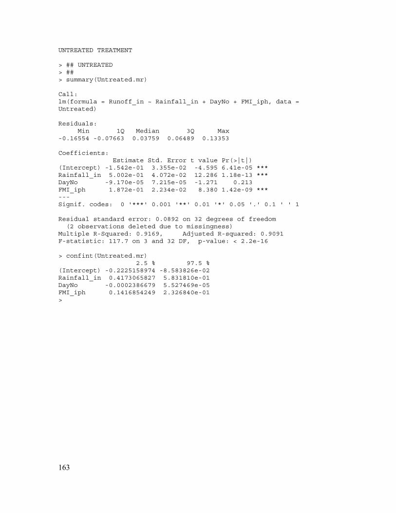
163

UNTREATED TREATMENT > ## UNTREATED > ## > summary(Untreated.mr) Call: lm(formula = Runoff_in ~ Rainfall_in + DayNo + FMI_iph, data = Untreated) Residuals: Min 1Q Median 3Q Max -0.16554 -0.07663 0.03759 0.06489 0.13353 Coefficients: Estimate Std. Error t value Pr(>|t|) (Intercept) -1.542e-01 3.355e-02 -4.595 6.41e-05 *** Rainfall_in 5.002e-01 4.072e-02 12.286 1.18e-13 *** DayNo -9.170e-05 7.215e-05 -1.271 0.213 FMI_iph 1.872e-01 2.234e-02 8.380 1.42e-09 *** --- Signif. codes: 0 '***' 0.001 '**' 0.01 '*' 0.05 '.' 0.1 ' ' 1 Residual standard error: 0.0892 on 32 degrees of freedom (2 observations deleted due to missingness) Multiple R-Squared: 0.9169, Adjusted R-squared: 0.9091 F-statistic: 117.7 on 3 and 32 DF, p-value: < 2.2e-16 > confint(Untreated.mr) 2.5 % 97.5 % (Intercept) -0.2225158974 -8.583826e-02 Rainfall_in 0.4173065827 5.831810e-01 DayNo -0.0002386679 5.527469e-05 FMI_iph 0.1416854249 2.326840e-01 >