Field Testing of Hand-Held Infrared … Testing of Hand-Held Infrared Thermography, Phase II Interim...
104
Interim Report Prepared for Missouri Department of Transportation December 2015 Project TRyy1144 Report cmr16-007 Field Testing of Hand -Held Infrared Thermography, Phase II TPF-5(247) Interim Report Prepared by Glenn Washer, Ph.D., P.E. Mike Trial Alan Jungnitsch, Graduate Research Assistant Seth Nelson, Graduate Research Assistant University of Missouri-Columbia Department of Civil & Environmental Engineering
Transcript of Field Testing of Hand-Held Infrared … Testing of Hand-Held Infrared Thermography, Phase II Interim...

Interim Report Prepared for Missouri Department of Transportation December 2015 Project TRyy1144 Report cmr16-007
Field Testing of Hand-Held Infrared Thermography, Phase II
TPF-5(247) Interim Report
Prepared by Glenn Washer, Ph.D., P.E.
Mike Trial Alan Jungnitsch, Graduate Research Assistant Seth Nelson, Graduate Research Assistant University of Missouri-Columbia Department of Civil & Environmental Engineering

TECHNICAL REPORT DOCUMENTATION PAGE
1. Report No.
cmr 16-007 2. Government Accession No.
3. Recipient’s Catalog No.
4. Title and Subtitle
Field Testing of Hand-Held Infrared Thermography, Phase II
5. Report Date
December 2015
6. Performing Organization Code
7. Author(s)
Glenn Washer, Ph.D., P.E.
Mike Trial
Alan Jungnitsch, Graduate Research Assistant
Seth Nelson, Graduate Research Assistant
8. Performing Organization Report No.
9. Performing Organization Name and Address
Department of Civil and Environmental Engineering
University of Missouri-Columbia
E2509 Lafferre Hall, Columbia, MO 65201
10. Work Unit No.
11. Contract or Grant No.
MoDOT project #TRyy1144
FHWA TPF-5(147)
12. Sponsoring Agency Name and Address
Missouri Department of Transportation (SPR) http://dx.doi.org/10.13039/100007251
Construction and Materials Division
P.O. Box 270
Jefferson City, MO 65102
13. Type of Report and Period Covered
TPF-5(147) Interim Report
(November 2011-December 2015)
14. Sponsoring Agency Code
15. Supplementary Notes
Conducted in cooperation with the U.S. Department of Transportation, Federal Highway Administration. MoDOT research reports
are available in the Innovation Library at http://www.modot.org/services/or/byDate.htm. This report and appendices are available
at http:// http://library.modot.mo.gov/RDT/reports/TRyy1144/ and http://www.pooledfund.org/Details/Study/475.
16. Abstract
This report describes research completed to develop and implement infrared thermography, a nondestructive evaluation (NDE)
technology for the condition assessment of concrete bridge components. The overall goal of this research was to develop new
technologies to help ensure bridge safety and improve the effectiveness of maintenance and repair. The objectives of the research
were to:
Quantify the capability and reliability of thermal imaging technology in the field
Field test and validate inspection guidelines for the application of thermal imaging for bridge inspection
Identify and overcome implementation barriers
The project provided hand-held infrared cameras to participating state Departments of Transportation (project partners), trained
individuals from these states in camera use, and conducted field tests of the technology. The reliability of the technology was
assessed, and previously developed Guidelines for field use were evaluated through systematic field testing. The implementation
of infrared thermography within the participating states was studied during the course of the research to identify implementation
challenges experienced by users of the technology. Finite element modeling of the thermal behavior of concrete under typical
environmental conditions was also completed to study the effects of defect depth and thickness and the effect of asphalt overlays.
Overall, the verification testing and results reported through the implementation study showed that the Guidelines provided
suitable conditions for detection of subsurface damage in concrete.
17. Key Words
Concrete bridges; Field tests; Nondestructive tests; Rehabilitation
(Maintenance); Infrared thermography
18. Distribution Statement
No restrictions. This document is available through the
National Technical Information Service, Springfield, VA
22161.
19. Security Classif. (of this report)
Unclassified.
20. Security Classif. (of this
page)
Unclassified.
21. No. of Pages
104
22. Price
Form DOT F 1700.7 (8-72) Reproduction of completed page authorized

Field Testing of Hand-Held Infrared Thermography, Phase II
Interim Report
December 2015
Prepared By: Glenn Washer, Mike Trial, Alan Jungnitsch (GRA) and Seth Nelson (GRA)
University of Missouri
Columbia, MO December 2015

ACKNOWLEDGEMENT OF SPONSORSHIP
This research was funded by the Missouri (MO) Department of Transportation
under pooled fund TPF – 5 (247). Twelve additional states participated in the pooled
fund, as indicated below. The authors gratefully acknowledge their support.
Texas, Minnesota, Oregon, Iowa, Pennsylvania, New York, Michigan, Georgia,
Wisconsin, Ohio, Kentucky, Florida
Disclaimer
The opinions, findings and conclusions expressed in this publication are not
necessarily those of the Departments of Transportation or the Federal Highway
Administration. This report does not constitute a standard, specification or regulation.
i
TABLE OF CONTENTS List of Figures .................................................................................................................. ii
List of Tables ................................................................................................................... v
List of Appendices ........................................................................................................... v
Executive Summary .........................................................................................................1
1 Introduction ..............................................................................................................3
Project Background ......................................................................................... 5 1.1
Summary of Tasks .......................................................................................6 1.1.1
Background on Infrared Thermography ........................................................... 8 1.2
Tools Developed for the Research .................................................................14 1.3
Bridge Inspection Planner .......................................................................... 14 1.3.1
Shared Data Site (SDS) ............................................................................. 16 1.3.2
2 Training of States ................................................................................................... 19
Training Delivery ............................................................................................20 2.1
Delivering the On-Site Training Sessions ................................................... 22 2.1.1
Evaluating Participants’ Satisfaction with the On-site Training .......................24 2.2
Selection of Cameras ................................................................................. 25 2.2.1
3 Verification Testing ................................................................................................ 27
4 Implementation Challenges .................................................................................... 41
5 Laboratory Testing ................................................................................................. 47
Adjustment of Wind Data................................................................................47 5.1
Background ................................................................................................ 49 5.1.1
Laboratory Testing of Wind Effects ............................................................. 51 5.1.2
Imaging and Pixel Resolution .........................................................................55 5.2
Introduction ................................................................................................ 55 5.2.1
Approach .................................................................................................... 56 5.2.2
Threshold Values for Imaging ..................................................................... 57 5.2.3
Illustration of Pixel Resolution .................................................................... 59 5.2.4
Modeling ........................................................................................................63 5.3
Numerical Model ........................................................................................ 64 5.3.1

ii
Simulation Results ..................................................................................... 67 5.3.2
Parametric Studies. ........................................................................................72 5.4
Model ......................................................................................................... 73 5.4.1
Effect of Asphalt Overlays .......................................................................... 80 5.4.2
Effect of the Materials in Delamination ....................................................... 82 5.4.3
Model Verification using Field Testing ........................................................ 84 5.4.4
Discussion of Numerical Modeling Results ................................................. 87 5.4.5
6 Conclusions ........................................................................................................... 89
Guideline Revisions .......................................................................................91 6.1
Ongoing and Future Research .......................................................................91 6.2
References .................................................................................................................... 93
LIST OF FIGURES
Figure 1. Schematic diagram of a bridge deck and overlay with debonding and
delamination damage. ..................................................................................................... 9
Figure 2. Schematic diagram of infrared energy emitted from damaged concrete
during heating (A) and cooling (B) cycles. ..................................................................... 11
Figure 3. Screen capture of the BIP web tool showing thermal inspection
recommendation. .......................................................................................................... 16
Figure 4. Screen capture of the "Tools and Resources" page of the project SDS.
...................................................................................................................................... 17
Figure 5. Data entry form used to submit applications of infrared thermography
to the SDS. .................................................................................................................... 19
Figure 6. Photograph of typical training activity using IR cameras in the field. ... 21
Figure 7. Thermal images of a delamination surrounding a deck drain, showing
thermal images in the afternoon (A) and the following morning (B); photograph of the
area (C) and ambient temperature conditions (D). ........................................................ 22
Figure 8. Map of the United States showing states where training was delivered
under the project. .......................................................................................................... 23

iii
Figure 9. Photograph of the FLIR T620 infrared camera (A) and the camera in its
carrying case, with additional batteries, lenses and accessories. ................................. 26
Figure 10: Photograph (A) and thermal image (B) showing locations of cores
removed from a bridge deck. ......................................................................................... 30
Figure 11: The cores taken from the delamination at L1 .................................... 31
Figure 12. Photograph of delaminated area of bridge deck showing delamination
depth measurements (A), and thermal image of the same area overlaid on a photograph
showing sounding results (B). ....................................................................................... 32
Figure 13. Schematic diagram of bridge deck exposed to solar loading, showing
effect of IR energy emitted at the soffit. ......................................................................... 33
Figure 14. Thermal image showing deck delamination on the soffit of the deck
appearing as a cold spot (A), and photograph of the same area of the soffit. ............... 34
Figure 15. Thermal image of a deck soffit showing the conduction effect on the
appearance of concrete delamination at the soffit. ........................................................ 35
Figure 16. Slab bridge in Ohio where IR testing was conducted. ...................... 36
Figure 17 Thermal images of delaminations in the soffit of a wide slab bridge,
showing morning (top) and afternoon (bottom) results. ................................................. 37
Figure 18. Thermal images showing damage along a longitudinal joint in a 159 ft
wide slab bridge. ........................................................................................................... 38
Figure 19: Ambient temperature for June 23, 2014 in Columbus Ohio ............... 39
Figure 20: Illustration of how thermal gradient can affect a thermal image. ........ 41
Figure 21. Graph showing correlation between experimental and NWS-reported
wind speed data for high wind speed conditions. .......................................................... 50
Figure 22. Schematic diagram of the test arrangement for evaluating wind
effects (A), and thermal image of the concrete test block showing subsurface target (B).
...................................................................................................................................... 53
Figure 23. Graph showing thermal contrast developed for subsurface targets
with varying air speed. ................................................................................................... 54
Figure 24. Maximum temperature differentials at 30 min. showing exponential
curve fit. ......................................................................................................................... 55

iv
Figure 25. Graph showing critical dimension as a function of observation
distance. ........................................................................................................................ 59
Figure 26. Photograph of test set-up for pixel resolution evaluation. ................. 60
Figure 27. Thermal images for the standard lens (A) and wide angle lens (B) at a
distance of 100 feet from the test specimen .................................................................. 61
Figure 28. Scene size in relation to distance from the camera lens. .................. 62
Figure 29. Area of one pixel in relation to distance from the camera lens. ........ 62
Figure 30. Images of a concrete test deck showing photograph (A) and thermal
images captured using B) wide angle, C) standard and D) telephoto lenses. ............... 63
Figure 31. Schematic diagram of concrete block modeled by FEM (A),
photograph of concrete test block in the field (B). ......................................................... 65
Figure 32. Environmental parameters as boundary condition in simulation on
November 5, 2007: (A) solar radiation; (B) ambient temperature; and (C) wind speed. 66
Figure 33. Typical thermal images of the thermal behavior for the South side of
the concrete block: (A) the model result at noon; (B) the field test result at noon; (C) the
model result at 8:00 p.m.; and (D) the field test result at 8:00 p.m. ............................... 68
Figure 34. FEM model results for the north and south sides of the test block,
showing typical results for surface temperature (A and B) and thermal contrasts (C and
D) .................................................................................................................................. 69
Figure 35. Thermal contrast determined from the numerical model and
measured in the field for A) solar loaded conditions and B) shady conditions. .............. 71
Figure 36. The basic geometry of the concrete model (geometry view in
COMSOL) ..................................................................................................................... 74
Figure 37. Three consecutive days of environmental parameters as a boundary
condition in simulation: (A) solar radiation; (B) ambient temperature; and (C) wind speed
...................................................................................................................................... 75
Figure 38. The time varying thermal contrast: (A) as a function of void depth, and
(B) as a function of void thickness ................................................................................. 76
Figure 39. (A) Effect of void depth on the maximum thermal contrast and (B)
Effect of void thickness on the maximum thermal contrast ............................................ 78

v
Figure 40. The time varying thermal contrast as a function of asphalt thickness:
(A) 51 mm deep void (B) 76 mm deep void. .................................................................. 81
Figure 41. Effect of asphalt thickness on the maximum thermal contrast. ......... 82
Figure 42. The time varying thermal contrast as a function of the materials
present in the void ......................................................................................................... 83
Figure 43. The digital image and the thermal image at 2:30 p.m. (obtained from
the field IR thermography testing) ................................................................................. 85
Figure 44. Thermal contrast as a function of void thickness for 51 mm deep void
...................................................................................................................................... 87
LIST OF TABLES
Table 1. Table showing the date that training was delivered in each state. ....... 23
Table 2. Table showing the results of surveys conducted following training in
each state. ..................................................................................................................... 24
Table 3. Results from the online survey of state DOTs regarding anticipated
implementation challenges. ........................................................................................... 42
TABLE 4. Example of estimation of maximum thermal contrast ........................ 79
TABLE 5. Material properties for case 2 involving different materials contained in
the void and the sound concrete. .................................................................................. 82
TABLE 6. The field test results including the coring results and the maximum
thermal contrast (ΔTmax) from thermography images. ................................................... 86
LIST OF APPENDICES
Appendix A: Guidelines for Thermographic Inspection of Concrete Bridges
Appendix B: Examples from the Shared Data Site
Appendix C: Verification Testing Summary Report
Appendix D: Presentations from the Training

vi

1
EXECUTIVE SUMMARY
This report describes research completed to develop and implement infrared
thermography, a nondestructive evaluation (NDE) technology for the condition
assessment of concrete bridge components. The overall goal of this research was to
develop new technologies to help ensure bridge safety and improve the effectiveness of
maintenance and repair. The objectives of the research were to:
Quantify the capability and reliability of thermal imaging technology in the field
Field test and validate inspection guidelines for the application of thermal imaging
for bridge inspection
Identify and overcome implementation barriers
The project provided hand-held infrared cameras to participating state
Departments of Transportation (project partners), trained individuals from these states
in camera use, and conducted field tests of the technology. The reliability of the
technology was assessed, and previously developed Guidelines for field use were
evaluated through systematic field testing. The implementation of infrared
thermography within the participating states was studied during the course of the
research to identify implementation challenges experienced by users of the technology.
Laboratory testing was conducted as a part of the research to evaluate various
parameters affecting the implementation of infrared thermography. A numerical model
using Finite Element Modeling (FEM) was developed and used to characterize key
parameters affecting the application of infrared thermography, such as the depth and
thickness of subsurface damage, the effect of asphalt overlays, and the effect of having
water, ice or epoxy filling a subsurface delamination. Web-based tools to support the
implementation of infrared thermography were also developed during the course of the
research to support field implementation of the technology and to provide a database of
field test results completed throughout the research.
The capability and reliability was demonstrated through field testing of the
technology and comparison with a secondary inspection technique, typically hammer
sounding but including coring and drilling into the bridge deck. In terms of quantifying
the capability and reliability of the technology, conclusions based on the data available

2
from the implementation study and verification study indicated that the technology was
reliable when implemented within the constraints of the Guidelines, if the depth of the
delamination was 3 inches or less. Overall, the verification testing and results reported
through the implementation study showed that the Guidelines provided suitable
conditions for detection of subsurface damage in concrete. Participants reported a high
degree of confidence in results when damage was detected.
The primary implementation barrier identified during the study was a lack of
available resources. For most participants, the technology worked effectively for the
purposes intended. Several participants indicated that the technology is being
integrated into condition assessment programs for the purpose of scoping renovation
activities and to focus inspection efforts where most needed.
3
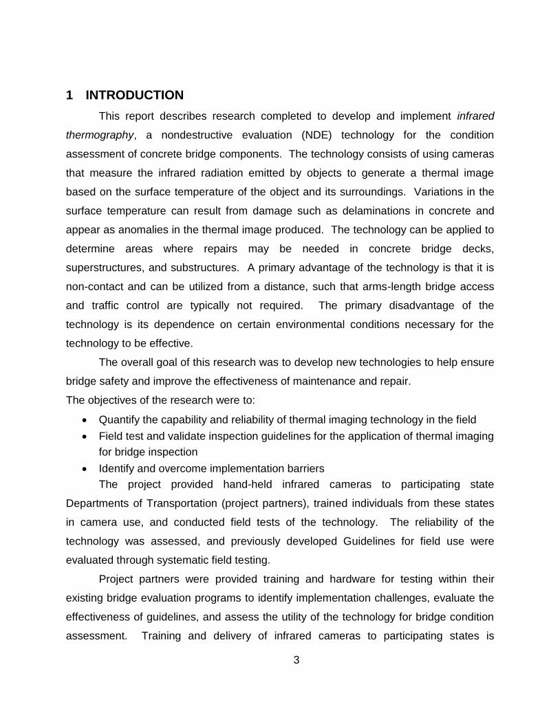
1 INTRODUCTION
This report describes research completed to develop and implement infrared
thermography, a nondestructive evaluation (NDE) technology for the condition
assessment of concrete bridge components. The technology consists of using cameras
that measure the infrared radiation emitted by objects to generate a thermal image
based on the surface temperature of the object and its surroundings. Variations in the
surface temperature can result from damage such as delaminations in concrete and
appear as anomalies in the thermal image produced. The technology can be applied to
determine areas where repairs may be needed in concrete bridge decks,
superstructures, and substructures. A primary advantage of the technology is that it is
non-contact and can be utilized from a distance, such that arms-length bridge access
and traffic control are typically not required. The primary disadvantage of the
technology is its dependence on certain environmental conditions necessary for the
technology to be effective.
The overall goal of this research was to develop new technologies to help ensure
bridge safety and improve the effectiveness of maintenance and repair.
The objectives of the research were to:
Quantify the capability and reliability of thermal imaging technology in the field
Field test and validate inspection guidelines for the application of thermal imaging
for bridge inspection
Identify and overcome implementation barriers
The project provided hand-held infrared cameras to participating state
Departments of Transportation (project partners), trained individuals from these states
in camera use, and conducted field tests of the technology. The reliability of the
technology was assessed, and previously developed Guidelines for field use were
evaluated through systematic field testing.
Project partners were provided training and hardware for testing within their
existing bridge evaluation programs to identify implementation challenges, evaluate the
effectiveness of guidelines, and assess the utility of the technology for bridge condition
assessment. Training and delivery of infrared cameras to participating states is

4
described in Chapter 2 of this report. A series of field tests, which included field
verification of results, were conducted by the project partners in cooperation with the
research team. These field tests evaluated and verified the capabilities and reliability of
the technology under field conditions. These data were used to validate and improve
the Guidelines and support practical implementations of the technology. Key findings
from the verification studies are included in Chapter 3 of this report.
The implementation of infrared thermography within the participating states was
studied during the course of the research to identify implementation challenges
experienced by users of the technology. The results of the implementation study are
reported in Chapter 4 of the report.
Laboratory testing was conducted as a part of the research to evaluate various
parameters affecting the implementation of infrared thermography. This included
laboratory studies related to wind-speed effects and the effects of using different lenses
on an infrared camera (i.e. wide angle, standard or telephoto) in terms of the detection
and identification of damage. A numerical model using Finite Element Modeling (FEM)
was developed and used to characterize key parameters affecting the application of
infrared thermography, such as the depth and thickness of subsurface damage, the
effect of asphalt overlays, and the effect of having water, ice or epoxy filling a
subsurface delamination. The results of the laboratory testing are reported in Chapter 5
of this report.
This report is Volume I of a two volume set, and includes research results to
date. These results include most of the research envisioned at the outset of the project.
During the course of the research, new technologies were identified that had different
capabilities from hand-held thermographic cameras. These technologies are currently
undergoing tests, and results will be reported in Volume II of this report. Also, additional
states joined the pooled fund to test and evaluate infrared thermography in their states.
This generally positive development resulted in some delay in completing all verification
testing necessary to meet the objectives of the project. Efforts to complete this
verification testing are ongoing. Additional analysis of results from these verification
tests, as well as additional analysis of data submitted by participating states

5
documenting their experiences with infrared thermography, is needed to meet all
objectives of the project.
Project Background 1.1
The research reported herein is the second phase (Phase II) of research
completed to develop infrared thermography as a practically implementable tool for
bridge condition assessment. During Phase I of the research program, Guidelines were
developed for field use of the technology. The Guidelines were based on results from
experimental testing completed at the University of Missouri. During the Phase I
research, a large concrete block was constructed with simulated subsurface damage at
various depths in the concrete. Thermal images of the block were captured
continuously over a time period of several months. These images were then analyzed
to evaluate the thermal contrast produced between the simulated defects and the intact
concrete in the block, as a result of varying ambient environmental conditions.
Statistical analysis of these data was used to identify suitable environmental conditions
for detecting subsurface damage in concrete using infrared thermography. The results
of this analysis were captured in “Guidelines for Thermographic Inspection of Concrete
Bridges.” These Guidelines describe conditions for utilizing the technology on concrete
exposed to direct sunlight, for example a bridge deck, and for areas not exposed to
direct sunlight, for example a soffit. These Guidelines (including revisions based on the
phase II research) are included in Appendix A of this report.
The research reported herein examines the implementation of these Guidelines,
and the thermal imaging technology as a whole, for practical implementation by State
Departments of Transportation (DOTs). In addition, field test results collected during
Phase I of the research showed numerous potential applications for the technology,
including bridge soffits, composite materials, and concrete decks. Further applications
for the technology were developed through the state-level testing conducted as part of
Phase II reported herein. In addition, field verification testing was conducted to better
characterize the effectiveness of the technology and to test the implementation of the
guidelines under practical and realistic field conditions. The implementation of the
technology was also studied as part of this phase II research.
6
Testing during Phase I also identified certain conditions that diminished the
capability of thermal imaging to easily and quickly assess subsurface damage in
concrete, in particular the presence of moisture in the concrete due to saturation and
the effect of high winds[1]. These conditions were evaluated during phase II through
limited laboratory study and numerical modeling.
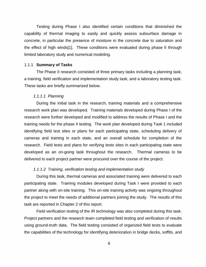
Summary of Tasks 1.1.1
The Phase II research consisted of three primary tasks including a planning task,
a training, field verification and implementation study task, and a laboratory testing task.
These tasks are briefly summarized below.
1.1.1.1 Planning
During the initial task in the research, training materials and a comprehensive
research work plan was developed. Training materials developed during Phase I of the
research were further developed and modified to address the results of Phase I and the
training needs for the phase II testing. The work plan developed during Task 1 included
identifying field test sites or plans for each participating state, scheduling delivery of
cameras and training in each state, and an overall schedule for completion of the
research. Field tests and plans for verifying tests sites in each participating state were
developed as an on-going task throughout the research. Thermal cameras to be
delivered to each project partner were procured over the course of the project.
1.1.1.2 Training, verification testing and implementation study
During this task, thermal cameras and associated training were delivered to each
participating state. Training modules developed during Task I were provided to each
partner along with on-site training. This on-site training activity was ongoing throughout
the project to meet the needs of additional partners joining the study. The results of this
task are reported in Chapter 2 of this report.
Field verification testing of the IR technology was also completed during this task.
Project partners and the research team completed field testing and verification of results
using ground-truth data. The field testing consisted of organized field tests to evaluate
the capabilities of the technology for identifying deterioration in bridge decks, soffits, and

7
other relevant areas of a bridge. The field testing of the technology generally consisted
of the following:
a. Collecting thermal images of a subject structure at several different times
of the day and night
b. Documenting the environmental conditions surrounding the testing
c. Evaluation/verification of thermal imaging results based on ground-truth
data. This activity established ground truth data on the characteristics of
the damage detected by thermal imaging. It was envisioned that the
ground truth would be evaluated using one of the following methods:
i. Forensic analysis of concrete components during demolition
ii. Coring of the member to identify the extent of damage
iii. Hammer sounding/chain drag
The selection of the verification methodology depended on the practical
limitations associated with the field test being conducted. Participating states were
expected to provide logistical and sampling support for the field testing, such as
sounding areas, obtaining samples, or assisting with obtaining samples if needed. In
most cases, hammer sounding was the primary method used to verify results. Key
results from the verification testing are included in Chapter 3 of this report.
The participating states utilized the IR cameras in the course of normal bridge
evaluations, according to the needs of the particular state. Project partners were
expected to utilize the technology within the context of their normal operating
procedures, to help identify potential barriers to implementation, improve training, and
facilitate broader application of the technology. Project partners provided results of
some of the field testing to the research team, including certain details surrounding the
testing such as bridge location, test conditions, and general construction information. A
web-based tool to support this activity was developed as part of the research.
During the implementation study task, the research team assessed the
implementation challenges identified by the project partners. The research team
collected and catalogued typical results from the field testing to assess the effectiveness
of the technology identify new applications, and document field test results as a
reference for future work. The results of the implementation study are reported in
Chapter 4 of this report.

8
1.1.1.3 Laboratory Testing Task
The research team at the University of Missouri also conducted laboratory testing
to address specific field test parameters for which better relationships were needed.
This laboratory testing included numerical modeling and experimental testing to assess
key parameters affecting the use of infrared thermography in the field. The testing was
focused on evaluating important parameters for the practical implementation of the
technology and improving the Guidelines for field use. The results of this task are
documented in Chapter 5 of this report.
Background on Infrared Thermography 1.2
Infrared thermography is capable of detecting subsurface damage in concrete
based on variations in thermal behavior of the concrete caused by the damage. Two
types of subsurface damage are typically the focus of thermographic inspections –
delamination in the concrete caused by corrosion and debonding between different
materials, for example, debonding of a concrete overlay from the concrete substrate.
Both subsurface delamination and debonding result in large planar flaws oriented
parallel to the surface of the concrete, as shown in Figure 1.
Reinforced concrete is commonly used as a construction material for highway
bridge structures. One of the most significant deterioration mechanisms in reinforced
concrete is corrosion of the embedded reinforcement steel which results in subsurface
damage to the concrete. As the steel corrodes, it expands, causing tension stresses in
the surrounding concrete [2]. These tensile stresses result in cracks or subsurface
fracture planes in the concrete at, or near, the level of the reinforcement, as shown in
Figure 1. These subsurface fracture planes are commonly referred to as delaminations.
As the deterioration process continues, a rupture between the delaminated region and
the main structural component can occur, which results in spalling of the concrete [3].
This damage typically occurs at the level of the reinforcing steel mat in the concrete,
normally at a depth of 1 to 3 in. in the concrete. For bridge decks such as depicted in
Figure 1, delamination may develop at the top layer of reinforcing, closest to the driving
surface of the bridge, or the bottom layer of reinforcing, producing a delamination
closest to the deck soffit.

9
Figure 1. Schematic diagram of a bridge deck and overlay with debonding and
delamination damage.
Some concrete bridge decks have overlay materials installed that cover the riding
surface of the bridge deck. Concrete, asphalt, and epoxy materials are commonly used.
These overlays may be used to improve the durability of the deck, improve the
serviceability of the deck, and/or extend the service life of the bridge. These materials
are chemically adhered to the surface of the concrete. The overlay material may
become debonded from the concrete substrate, creating a debonding defect at
concrete/overlay interface. As deterioration progresses, the debonded areas expand
and can propagate to the surface, creating spalls in the deck.
Spalling of concrete can affect concrete bridge safety and serviceability. Spalling
of the concrete deck surfaces can affect the ability of the deck to carry traffic at normal
speeds, may accelerate the overall deterioration of the deck, and can require
maintenance or renovation activities that disrupt traffic [4, 5]. Concrete spalling on the
underside of an overpass bridges can be a safety hazard to traffic passing below if
concrete falls from the bridge into moving traffic [6]. For these and other bridge
components, delaminations and spalling are indicative of deterioration and active
corrosion. Spalling of concrete also exposes reinforcing steel to the ambient
environment, often accelerating the rate of deterioration. As a result, locating and
defining the extent of subsurface damage that leads to spalling provides important
information regarding the current condition and future repair needs.

10
Conventional methods of identifying subsurface delaminations include chain
dragging and sounding with hammers or rods. These methods necessitate hands-on
access to the surfaces being inspected, are subjective, and may be inaccurate [7, 8].
For highway bridges, achieving the access necessary to reach key bridge components
for sounding can require special access equipment, such as man lifts, and often
requires lane closures that disrupt traffic. In the case of chain dragging, only bridge
decks and other horizontal surfaces can be inspected. Due to the access requirements
of these methods and their inherent subjectivity, nondestructive evaluation (NDE)
techniques, such as thermography, sonic testing (impact echo (IE)), and ground
penetrating radar (GPR) technology, have been explored as a means of reducing the
access requirements and improving the quality of inspections [3, 5, 9-12]. Sonic testing,
usually implemented using an IE approach, requires impact at the surface of the
material being tested. Consequently, hands-on access to the surface to be assessed is
always required. In the case of GPR, air-coupled antennae can be used to reduce or
even eliminate required traffic control for some bridge decks, but generally requires
close access of about 1 m to the surface to be implemented. Implementation of air-
coupled GPR for deck soffits, primary members, or substructures is not practical due to
the access requirements. Ground-coupled antennae may be used for soffits, primary
members, or substructures, but has similar access challenges. Of these technologies,
infrared thermography is the only method that does not require direct access to the
surface under inspection because images can be captured from a large distance using
appropriate lenses.
Thermography employs infrared sensors to detect thermal radiation emitted from
objects, and creates an image of surface temperatures based on the emitted radiation.
The energy of emitted radiation is expressed by using Stefan Boltzmann Law as
(1)
in which is infrared emissivity of the object, is Stefan Boltzmann constant (5.67 x 10-
8 W m-2 K-4), and T is the surface temperature. In concrete, subsurface anomalies such
as delaminations interrupt heat flow producing localized differences in the surface
temperature. These localized variations in surface temperature affect the amount of
infrared radiation emitted from the surface, as shown schematically in Figure 2. As

11
concrete warms (Fig. 2A), the surface temperature above a delamination is higher than
the surface temperature of the sound concrete. Conversely, as concrete cools (Fig.
2B), the surface temperature of the concrete above a delamination may be lower than
the temperature of the surrounding concrete [13]. The location of subsurface anomalies
can be identified by analyzing the surface temperature variations. These surface
temperature variations were examined in terms of thermal contrast to perform
quantitative analysis of data in the study. Thermal contrast, ΔT, is defined as
(2)
where Tvoid is the surface temperature above a void area (i.e subsurface defect such as
a delamination) and Tsound concrete, the surface temperature in the intact area of the
concrete.
Figure 2. Schematic diagram of infrared energy emitted from damaged concrete during
heating (A) and cooling (B) cycles.
The effectiveness of thermographic imaging is highly dependent on
environmental conditions at the time, and prior to, when a thermal image is captured.
The thermal gradient in the concrete that results from certain environmental conditions,
such as solar loading, drives conductive heat transfer in the concrete. Disruptions in
heat flow are caused by subsurface damage, resulting in variations in surface
temperature, which can be used to identify the location of the subsurface damage in a
thermal image. Suitable environmental conditions affecting the concrete at the time of,
and prior to, imaging is needed to make subsurface damage detection effective.
Significant environmental parameters that affect the thermal gradient in the concrete are
solar radiation, cloud cover, ambient temperature, wind speed, and surface moisture
[14].

12
Previous research on the use of infrared thermography for bridge inspection has
described the environmental conditions affecting thermographic detection of subsurface
damage. Early studies by Manning found that delaminations in concrete decks could be
detected using thermography in field tests [15]. His studies found that the delamination
could be detected over a wide range of ambient temperatures, since the delaminated
areas heat up faster due to solar loading, and could develop surface temperatures from
1°C to 3°C (1.8° to 5.4° F) higher than the surrounding areas. Manning found that in
ideal summer conditions with no clouds or wind, surface temperature differences (i.e.
thermal contrasts) as large as 4.5⁰C (8.1°F) could be found between delaminated and
solid sections of a concrete bridge deck. The temperature differential was reduced by
wind, cloud cover, and high humidity [16].
Maser investigated the potential of NDE technologies to assess the level of
deterioration of concrete bridge decks using radar and infrared thermography [3]. The
study used theoretical models to evaluate the effects of variable depth of concrete
cover, thickness, and materials for a subsurface void under a certain set of
environmental variables. The thermal response was analyzed using a one-dimensional
transient heat transfer model. Analytic studies revealed that the ability of infrared
thermography to detect delaminations depended on the thickness of the
void/delamination, the concrete cover above the void, and if there was an asphalt
overlay applied. The temperature difference produced by a delamination for bare
concrete ranged from 3°C to 8°C (5.4° to 14.4° F) according to the model. The model
was not compared with experimental results.
The ASTM Standard Test Method for Detecting Delaminations in Bridge Decks
Using Infrared Thermography describes environmental conditions for detecting
delamination in bridge decks[17]. This standard indicates that thermographic imaging is
dependent on the amount of direct sunlight, the ambient temperature change, and wind
speed. The Standard provides generalized guidance on appropriate conditions for
detecting delaminations in bridge decks.
The Phase I research studied the effect of environmental conditions such as
direct solar loading, ambient temperature variation, wind speed, and humidity on the
surface temperature of a concrete block containing subsurface voids at different depths.

13
[1] The concrete block was constructed in a large field and aligned such that the south
face of the block was exposed to direct solar loading, while the north side of the block
was not exposed to direct solar loading. Subsurface delaminations were simulated
using Styrofoam targets at various depths. A FLIR S65 camera was used to capture
thermal images of the surface of the block at 10 minute time intervals, 24 hours a day
for three months on each side of the block. The thermal sensitivity of the camera is
0.08⁰C, coupled with a 320 x 240 pixel focal plane array to provide real-time imaging
display and storage.
It was found that direct, uninterrupted solar loading, and low wind speeds
provided optimum conditions for detection of targets for the south side of the block,
while high rates of change in ambient temperatures (greater than 3° F per hour) were
needed to create thermal contrast for the north side of the block, where no solar loading
was present[1, 18]. Quantitative values for the amount of solar loading, average wind
speeds and ambient temperature variations were determined statistically from the
experimental results and used to develop guidelines for the use of thermography in the
field . The experimental results of this study provided the input and verification data for
the present work described herein.
These investigations indicate the importance of environmental conditions on the
effectiveness of thermography for detecting delaminations in concrete bridge
components. For practical inspection scenarios, the environmental conditions obviously
cannot be controlled and will vary on a day to day basis. An accurate numerical model
that could estimate the anticipated level of thermal contrast based on the anticipated
depth of a delamination and for a given set of actual environmental conditions would
provide an important tool for the inspection of concrete bridge components. Such a
model could be used to assess the combination of solar loading, ambient temperature
change, and wind speed during, or leading up to, a field inspection, to predict the
anticipated thermal contrast for a delamination at a given depth. These data could then
be used to evaluate if sufficient conditions exist to make it likely that a delamination
would be detected, to estimate the depth of a detected delamination based on the
thermal contrast, and to determine if detected thermal differences correspond with

14
actual subsurface defects. A numerical model was developed and tested during the
research.
Tools Developed for the Research 1.3
Several tools were developed during the research to support the implementation
of infrared thermography. These included a web-based tool to provide key weather
data in the field, and a database of field-testing results. This portion of the report
describes the tools that were developed to support the research.
Bridge Inspection Planner 1.3.1
A web-based tool for planning of thermal inspections was developed during the
research, based on a prototype that had been developed during the phase I research.
The objective of this tool was to provide inspectors real-time data in the field regarding
the suitability of weather conditions for conducting thermal inspections. In summary, the
Bridge Inspection Planner (IR-BIP) uses the location features of a smart phone or other
computer to identify the location of the inspector. These data are then used to query
appropriate databases of weather information provided by a network of weather stations
located throughout the United States. These weather stations report weather conditions
such as wind speed, temperature and precipitation on an hourly basis. The IR-BIP data
displays ambient temperatures over the previous ~15 hrs and the predicted weather at
that location for the future ~35 hrs. These data are displayed as an x-y plot of ambient
temperature as a function of time. Wind speed and precipitation data are also collected
and stored.
These data are then utilized to compare the current conditions with the condition
described in the Guidelines, including required temperature changes and wind speed.
Time intervals for inspection described in the Guidelines, based on the delamination
depth of two inches, are displayed as shaded regions on the ambient temperature
graph. These data are analyzed to make a recommendation regarding the suitability of
the weather conditions for thermal inspections for sunny and shaded conditions, as well
as night time inspection. A recommendation is displayed as an icon on the screen, as
shown in Figure 3. This figure shows a screen capture from a smartphone displaying
the BIP, for the location of Columbia, MO. As shown in the figure, the current sky

15
conditions and an interactive map are also displayed. In the figure shown, check marks
indicate that the weather conditions are suitable for inspections for both sunny and
shaded daytime conditions. For nighttime inspections, conditions are not suitable
because the current time was outside the required time interval for a nighttime
inspection as described in the Guidelines. A circle and backslash icon is displayed for
nighttime inspections.
The BIP has a number of unique features and enhancements compared to the
prototype tool developed under phase I. These include automated algorithms to
analyze the weather conditions and provide a real-time recommendation for inspection.
The IR-BIP displays key data supporting the recommendation, such as the rate of
ambient temperature change and average winds speeds over the preceding three hour
time interval.
In addition, the BIP shows the predicted weather at a given location for the
following day. These data are intended to be used for planning of future inspections.
The interactive map that is displayed allows a user to locate areas where inspection
may be conducted the following day by dragging a cursor on the screen. The
appropriate zip code for an area can also be used. The predicted ambient temperature
variations at the identified location are then displayed, to allow the user to assess the
suitability of predicted weather patterns for inspections to be conducted the following
day.

16
Figure 3. Screen capture of the BIP web tool showing thermal inspection
recommendation.
Shared Data Site (SDS) 1.3.2
A web site was developed to support the research by providing a location to post
key information and to allow participating states to upload results to be shared with
others. The objectives of the web site were to provide a centralized location for the
dissemination and storage of important study information and to develop a searchable
database of successful applications of thermal imaging. The database is intended to
provide a reference for future users to assess the applicability of the technology for
different situations within their state and to provide easily accessible examples. The
entries made by the states are viewed by the research team as the images are added.
Quality control is performed by discussing with the uploading inspectors what
verification method was used to compare with the infrared results.

17
In June 2012, the research team established the shared data site (SDS), located
at thermo.missouri.edu. Since that time, more than 100 entries have been uploaded to
the site by participants from states currently participating in the project and the research
team. This portion of the report describes this web site and its functionality.
The web site features a “Tools and Resources” page that contains key project
information. Figure 4 shows a screen capture of the “Tools and Resources” page,
illustrating the appearance of the page and noting key data located there. These data
include the Guidelines for the thermal imaging and operational guidance on use of the
T620 cameras used as part of the study. The slide presentations that were used for
training can be downloaded from links located on this page for use by participants for
further training or review. A link to the BIP planner is also available on this page, as
shown in Figure 4.
Figure 4. Screen capture of the "Tools and Resources" page of the project SDS.

18
Slides presented during the project webinars and two videos of infrared imaging
are also available on this page. These videos illustrate the application of thermal
imaging for bridge decks and bridge soffits.
An entry search tool is located in the lower right corner of the page depicted in
Figure 4. This tool allows a user to search the submitted entries via search criteria
including the type of element shown in an image (deck, deck soffit, substructure, etc.),
the entry month, and state providing the image or location of the bridge.
The SDS entry form shown in Figure 5 allows a user to upload thermal images
from specific bridge applications. On this page, a user enters the location (GPS
coordinates) and date of the inspection. An automated tool retrieves the weather
conditions, based on the location and date entry, and reports the ambient temperature
and wind conditions at the location and time that the images were captured. Each entry
has bridge location and weather information at the time of imaging and typically includes
multiple thermal images and photographs of a bridge element. The weather data
retrieved for the submitted images is displayed in graphical format in the entry, and is
also displayed in a table of numerical results. This allows a user to copy the weather
data in numerical form for further analysis or to develop customized presentation
formats for the data.
As noted previously, the SDS has more than 100 entries showing implementation
of thermal imaging for the detection of subsurface damage in concrete. Additional
entries are being made to the SDS throughout the remainder of the project. These data
are being retained to support future implementation of infrared thermography and as a
technology transfer tool. The data can be searched for examples of thermal imaging
applied to bridge decks, soffits, and substructures as well as applications for imaging of
composite overwraps and other applications of the technology. The data on the website
can also be analyzed to evaluate the ambient weather conditions.

19
Figure 5. Data entry form used to submit applications of infrared thermography to the
SDS.
2 TRAINING OF STATES
This chapter of the report addresses the training phase of the project. The
training phase consisted of developing and delivering on-site training to individuals from
each of the participating states. The training was designed to familiarize participants
with the theory and application of infrared thermography, explain how effective thermal
images can be produced in the field, and to describe the necessary weather conditions
for effective thermal imaging in the field. The tools and resources developed through
the project were also described during the training sessions. The primary technology
developed under this portion of the study was the training modules and slides, which
are included herein as Appendix D to the report. The training materials such as

20
Powerpoint slides and a camera user’s guidebook were also made available to
participating states on the project’s SDS (thermo.missouri.edu.).
Training Delivery 2.1
The project training was delivered at state Department of Transportation training
facilities and at nearby in-service bridges. Training was typically conducted over a 1.5
day time period. This included ½ day of classroom training with instruction supported
by a series of powerpoint slides presentations, and two ½ day time periods available for
field testing and training using the infrared cameras for practical situations.
Training materials were developed by the research team during the period
January 2, 2012 through March 21, 2012. The classroom presentation was divided into
five modules:
Module 1, an introduction to thermography
Module 2, the theoretical background of heat transfer
Module 3, the environmental factors affecting infrared imaging
Module 4, making a good infrared image
Module 5, using the infrared camera
All five modules are presented and discussed in the first four hour classroom
session. After lunch, the instructors and participants visited an in-service bridge
suspected of having subsurface delaminations in the concrete. During these visits,
participants practiced imaging areas suspected of delamination with the infrared camera
in afternoon conditions, as shown in Figure 6. The field training activities were typically
supported using Ipad and/or mobile phones with applications that allowed multiple
participants to view the thermal images being observed on the cameras during the
testing. This allowed multiple participants to view the thermal images being produced in
real-time. During the course of the field training, camera setting and imaging
parameters were reviewed to allow participants to gain an understanding of the use and
application of the cameras.

21
Figure 6. Photograph of typical training activity using IR cameras in the field.
During the second day of training, images from the preceding day’s practice were
sometimes examined and discussed. Typically, the research team and students
returned to the same bridge and practiced taking infrared images in morning conditions.
This training pattern allowed participants to observe the same bridge areas under
different ambient weather conditions.
An example of visiting the same bridge in the afternoon and the following
morning during the training is shown in Figure 7. The figure shows thermal images of
the soffit of deck slab in the area of a deck drain (Figure 7 A and B), a photograph of the
same area (Figure 7C), and a graph of the ambient temperature conditions at the bridge
(Figure 7D). Figure 7A shows the thermal signature from a large delaminated area
surrounding a deck drain in the afternoon, during the positive ambient heating cycle.
Under these conditions, the thermal signature of the delamination appears warmer than
the surrounding, intact concrete. As shown in Figure 7D, image 7A was captured at ~2
pm. Figure 7B was captured the following morning at ~9:00 am, following the cooling of
ambient temperatures at the bridge. Under these conditions, the thermal signature of
the delamination appears cooler than the surrounding, intact concrete. The damage in
this area was confirmed using hammer sounding. Observing the same area during
afternoon and morning conditions assists students with understanding the effect of
ambient conditions on test results, and also helps confirm the results of the previous
day’s image interpretation.

22
Delivering the On-Site Training Sessions 2.1.1
Training sessions were held in each of the 12 participating states that received
cameras under the project. This training was completed during the period March 26,
2012 through April 29, 2014. A thirteenth state, Missouri, participated as program
manager for the project but, no training was performed in Missouri. Figure 8 shows a
map of the United States with the participating states highlighted to show the broad
geographic distribution of states where training was delivered under the project. The
dates of training in each state are shown in Table 1.
Figure 7. Thermal images of a delamination surrounding a deck drain, showing thermal
images in the afternoon (A) and the following morning (B); photograph of the area (C)
and ambient temperature conditions (D).

23
Figure 8. Map of the United States showing states where training was delivered under
the project.
A total of 110 people received training. Each participant in the training was
provided a workbook which included all the training slides used in the instruction and a
copy of the infrared camera use guidelines developed by the research team in August
2009 as part of Phase I of this project. Each participant received a certificate for 1.2
continuing education units from the University of Missouri.
Table 1. Table showing the date that training was delivered in each state.
State Dates of Training
Texas March 26-27, 2012
Minnesota April 23-24, 2012
Oregon May 21-23, 2012
Iowa June 4-6. 2012
Pennsylvania July 16-17, 2012
New York July 18-19, 2012
Michigan August 14-15, 2012
Georgia September 17-18, 2012
Wisconsin October 22-23, 2012
Ohio May 6-7, 2013
Kentucky July 31 – Aug 1, 2013
Florida April 28-29, 2014

24
Evaluating Participants’ Satisfaction with the On-site Training 2.2
At the conclusion of each training session, each participant was asked to
complete an evaluation of the training which consisted of 17 questions covering three
areas: satisfaction with the training (a higher percentage indicates greater satisfaction),
which module of the training was most/least useful, and the participant’s expectation of
the ease of using infrared cameras in future bridge inspections (a higher percentage
indicates the respondent expects camera use to be relatively easy). The survey
featured a rating scale (low to high) that was averaged among participants in each state
to determine the data shown Table 2. The results of the survey indicated that Module 1,
Introduction, was the least useful of the training modules and Module 4, Making a Good
Image, was the most useful module, although results varied considerably between
participants. No training evaluation was done at Texas DOT session due to an
oversight.
Table 2. Table showing the results of surveys conducted following training in each state.
State DOT
Satisfaction
with training
(%)
Most/Least
useful module
Will IR camera
use be easy?
(%)
No. of students
No. of
evaluations
received
MN 75 4/1 75 8 4
OR 89 4/1 82 10 10
IA 66 4/1 69 6 6
PA 88 4/1 81 10 4
NY 75 4/1 72 8 8
MI 84 4/1 76 22 16
GA 75 4/1 83 5 5
WI 77 4/1 75 9 8
TX - - - 7 0
OH 80 4/1 70 14 10
KY 85 4/1 80 10 8
FL 80 4/1 75 8 3

25
The training phase of the project was successfully executed on time and within
budget. A total of 110 employees of twelve state Departments of Transportation were
instructed in the background of thermal imaging and trained in the use of an infrared
camera. A FLIR T620 camera was provided to each participating state DOT and that
camera was used to image suspected subsurface flaws in concrete bridge decks at a
bridge managed by the state DOT. State DOT personnel reviewed images made at the
practice session at that bridge and were able to practice identifying and uploading
images to the project shared-data site.
Results of participant surveys conducted during the training indicated that the
training met the needs and expectations of the states involved in the research. The
training slides for each module of the training are included herein as Appendix D.
Selection of Cameras 2.2.1
During the project planning phase, the research team developed evaluation
criteria for infrared imaging cameras to be purchased by the project and provided to
participating state DOTs. The criteria that met the objectives of the project were:
accuracy, ease of camera use, image management and exportability, and cost. An
availability survey was conducted and the research team found that there were many
low-accuracy, low-cost, hand held and fixed-position thermal detection devices, but only
a few more sophisticated hand-held thermal imaging systems with the accuracy, ease of
use, and reasonable cost that the project required.
Desirable characteristics for the infrared camera to be used in the research
included a thermal sensitivity of ~0.05° C, such that thermal variations of less than 1°C
were easily detectable by the imaging device. This characteristic was based in part on
the result of the phase I research, which was conducted using a camera with the
thermal resolution of 0.08° C. A pixel resolution 640 by 480 pixels was desirable, to
provide adequate resolution to easily define the boundaries of damage in the thermal
image at a reasonable distance.
Other features that the research team felt would make the system appealing to
novice users include autofocus (along with the option for manual focus), a spot
temperature measurement capability, manual thermal image contrast and temperature

26
span adjustment on-screen, and the ability to take simultaneous photographs and
thermal images of an object. The images should also be easily exportable in standard
software formats. A comparison of three of the industry leading hand-held IR systems,
Fluke ,FLIR, and Jenoptik was completed as part of the research. The FLIR T620 was
chosen based on the evaluation criteria identified.
Each camera included a carrying case, two batteries, a charger, and a wide-
angle lens. Figure 9 shows a photograph of the FLIR T620 camera (A) and the carrying
case provided with the camera (B). This camera set has proven capable of meeting the
needs of the project and has been well received by state DOT personnel.
Figure 9. Photograph of the FLIR T620 infrared camera (A) and the camera in its carrying
case, with additional batteries, lenses and accessories.
The results of this camera selection have been positive. None of the state DOT
trainees have complained that camera use was so complex it interfered with easy use.
Image interpretation and exportability were straightforward. The FLIR T620’s relatively
large view screen and the articulating lens have been convenient for users. There have
been no durability problems or repairs required to date.
27
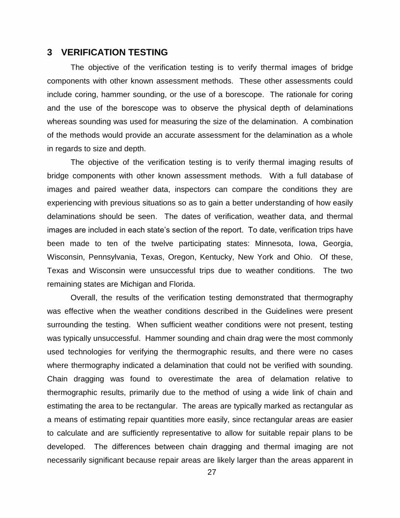
3 VERIFICATION TESTING
The objective of the verification testing is to verify thermal images of bridge
components with other known assessment methods. These other assessments could
include coring, hammer sounding, or the use of a borescope. The rationale for coring
and the use of the borescope was to observe the physical depth of delaminations
whereas sounding was used for measuring the size of the delamination. A combination
of the methods would provide an accurate assessment for the delamination as a whole
in regards to size and depth.
The objective of the verification testing is to verify thermal imaging results of
bridge components with other known assessment methods. With a full database of
images and paired weather data, inspectors can compare the conditions they are
experiencing with previous situations so as to gain a better understanding of how easily
delaminations should be seen. The dates of verification, weather data, and thermal
images are included in each state’s section of the report. To date, verification trips have
been made to ten of the twelve participating states: Minnesota, Iowa, Georgia,
Wisconsin, Pennsylvania, Texas, Oregon, Kentucky, New York and Ohio. Of these,
Texas and Wisconsin were unsuccessful trips due to weather conditions. The two
remaining states are Michigan and Florida.
Overall, the results of the verification testing demonstrated that thermography
was effective when the weather conditions described in the Guidelines were present
surrounding the testing. When sufficient weather conditions were not present, testing
was typically unsuccessful. Hammer sounding and chain drag were the most commonly
used technologies for verifying the thermographic results, and there were no cases
where thermography indicated a delamination that could not be verified with sounding.
Chain dragging was found to overestimate the area of delamation relative to
thermographic results, primarily due to the method of using a wide link of chain and
estimating the area to be rectangular. The areas are typically marked as rectangular as
a means of estimating repair quantities more easily, since rectangular areas are easier
to calculate and are sufficiently representative to allow for suitable repair plans to be
developed. The differences between chain dragging and thermal imaging are not
necessarily significant because repair areas are likely larger than the areas apparent in

28
the thermal image due to incipient damage along the edges of a delamination.
Regardless, it was found during the verification testing that sounding provided a very
suitable and practical tool to verify IR results. When weather conditions were suitable
for IR, there were not areas detected by chain drag (or sounding with a hammer) that
were not detected with IR. For example, if the angle of the sun precluded effected IR
imaging because the temperature gradient across the surface of the concrete was too
large to allow for an effective image to be captured. This occurs primarily in
substructure elements, where portions of the element are shaded and portions are in full
sun. An example of this situation is shown in Section 3.1.1.4, which describes different
scenarios where IR imaging was found to be ineffective.
Samples from the verification testing for each of the states visited are included in
Appendix C. In this appendix, a brief description of each of the verification tests are
reported along with selected data. A few selected highlights from the verification testing
are included herein to provide key results. These include the effects of delamination
depth, the appearance of deck delaminations in the soffit of the bridge, and the use of
thermography for a very wide structure where ambient temperature variations along the
centerline of the structure are diminished due to the large extent of the superstructure.
3.1.1.1 Effect of Delamination Depth
The depth at which a delamination occurs has a significant effect on the resulting
thermal contrast apparent in an image. A deeper delamination will have a smaller
thermal contrast, relative to intact concrete, than a shallow delamination. A
delamination of varying depth will also have varying contrast. The relationship between
the depth of a delamination and the magnitude of the thermal contrast was well
described by the research conducted during Phase I of the project in which targets at
different depths in a concrete block were monitored using a thermal camera. This effect
was illustrated in the field during verification testing in the state of Minnesota. During
the verification testing, three cores were removed from a portion of the deck where a
delamination showing varying thermal contrast had been detected. Figure 10A shows
the core locations superimposed on a photo of the area. The areas imaged had a
small, very hot area, which is shown as white in the IR image (Figure 10B), a large

29
yellow area around the white, and areas of pink around the outer limits of the
delamination. Note that there was also some residual asphalt material on the surface
that was black in color, which resulted in increased heating of that area due to
absorption of solar loading. Delamination is still apparent in this area due to the thermal
contrast created at that location, as shown in Figure 10B.
The first sample (L1S1) was removed from an area appearing as white (area of
largest thermal contrast) in Figure 10B. Typically, the highest thermal contrast indicates
an area closest to the center of a delamination or an area where delamination is at a
shallow depth. The second core (L1S2) was taken at the edge of the delamination that
showed only a slight increase in the thermal contrast from the solid concrete around it.
In the IR image shown in Figure 10B, the contrast between the core location and the
solid concrete was less defined. This is because the thermal contrast in this area was
only ~0.6°F. A thermal difference of less than one degree units can be difficult to detect
visually during the time of the inspection, even with a very small span setting; this is
because surface cracks, paint, sand, and other debris can appear to be at a slightly
different temperature than the solid concrete, causing noise in the image. This
difference in temperature was determined to be caused by a subsurface defect since
this area appeared to be clear of any debris and the surface color of the concrete was
consistent with the majority of the bridge deck.
A third sample (L1S3) was taken from an area that had a less distinct difference
in thermal contrast from sample L1S1 and more distinct thermal contrast than sample
L1S2. This shows up as mostly yellow with some pink in image B below.

30
Figure 10: Photograph (A) and thermal image (B) showing locations of cores removed
from a bridge deck.
These thermal differences within the same delamination were due in part to the
variation in cover above the delamination as shown in Figure 11, which shows a
photograph of the three core samples. Sample L1S1 was taken just off the area that
appears white in the IR image; in this area, the delamination was the closest to the
surface, approximately 1.875 in. deep in the concrete as determined from the core
sample. Sample two (L1S2) had the lowest thermal contrast of the three samples and
the core had the largest amount of cover above the delamination, 2.625 in. This datum
is consistent with the increased depth of the delamination, and the location of the core
near the edge of the delamination where thermal contrasts are typically diminished
regardless of depth. Core L1S3 indicated 2.375 in. of concrete cover, and is also near
the edge of the delamination.

31
Figure 11: The cores taken from the delamination at L1
The effect of depth of the delamination was further explored through a verification
test conducted in Iowa. In this case, the depth of the delamination was determined by
drilling into the surface of the deck and using a borescope to assess the depth of the
delamination. Figure 12A shows the depth measurements taken using a borescope at
each location where a measurement was recorded. Figure 12B shows the
corresponding thermal image superimposed on a photograph of the imaged area.
Hammer sounding was also conducted to determine the boundaries of the delamination
and the sounding results are shown with a red line for clarity. A foil-tape marker that
was used to as a research tool is also shown in the image. This foil marker creates a
consistent thermal contrast in the image, regardless of the surrounding environmental
conditions, due to the difference in emissivity between the foil and concrete. The
marker was used to assist the research team in confirming spatial locations on the
bridge; a series of markers in unique patterns was placed at 20 ft. intervals on the
bridge prior to testing.
The thermal image shown in Figure 12B appears to indicate two separate
delaminations. However, the delamination is actually one large delamination of variable
depth. According to the depth measurements shown in Figure 12A, the middle portion
of the delamination has a depth of ~3.1 - 3.5 in. This area has different thermal contrast
compared with the edge of the area where measured depths were ~1.25-1.6 in.

32
Figure 12. Photograph of delaminated area of bridge deck showing delamination depth
measurements (A), and thermal image of the same area overlaid on a photograph
showing sounding results (B).
These data illustrate field examples of the effect of depth of the delamination on
the thermal images produced. To mitigate this effect, thermal inspection can be
performed later in the heating or cooling cycle for the deck when deeper features are
more easily imaged.
3.1.1.2 Imaging of Soffit Areas
The imaging of delamination in the soffit area of bridge decks is described in the
Guidelines for inspections conducted in shaded conditions. It was found during the
verification testing that for bridge decks exposed to solar loading on the surface, as
illustrated in Figure 13, the behavior was different than described in the Guidelines.
When a bridge deck is exposed to direct solar loading over the course of the day, the
resulting warming of the deck conducts through the thickness of the concrete deck. As

33
a result, the heating from the sun affects the IR energy emitted from the soffit. When
there is a discontinuity in the conduction path, the heating is interrupted, reducing the IR
energy emitted from the soffit area, as illustrated in Figure 13. As a result, delamination
in the soffit areas appear as cold spots, rather than hot-spots as envisioned by the
Guidelines.
Figure 13. Schematic diagram of bridge deck exposed to solar loading, showing effect of
IR energy emitted at the soffit.
There were numerous examples of this conduction effect experienced during the
field testing of IR cameras with state DOTs. Figure 14 shows an example of this effect
from the previous delamination imaged in Figure 13. This image of the soffit area
shows the large delamination, which is at depths of 1.6 to 4.5 in. from the top surface of
the deck, as a large cold area in the soffit of the bridge deck. These data were captured
at 3:22 pm in the afternoon.
The conduction effect was observed for both delamination closest to the surface
of the bridge deck as well as delamination closest to the soffit surface. It is not possible
to approximate the depth of the delamination from the soffit surface from a single image
showing the conduction effect. For example, if it was desirable to determine if the
delamination were closest to the deck surface or the soffit surface, a single image
showing the conduction effect does not appear to provide sufficient information to make
that determination. However, observation of the area earlier in the heating cycle, or
during the overnight cooling period, would provide sufficient data to determine if the
delamination were closest to the deck surface or closest to the soffit surface.

34
Figure 14. Thermal image showing deck delamination on the soffit of the deck appearing
as a cold spot (A), and photograph of the same area of the soffit.
A second example is shown in Figure 15. This figure shows a thermal image of
the soffit area of a bridge in the area of a longitudinal joint. A parapet on the bridge
deck (not shown in the image) creates an area in the soffit where temperatures are
relatively cooler, due to the shadowing effect of the parapet and its thermal mass. In
deck areas adjacent to the parapet, the heating from the sun has conducted through the
deck. In the figure, a delamination in the soffit area of the deck is encircled. Four
temperature measurements were made in this area and are labeled A, B, C and D.
These data show that the nominal temperature of the deck at point A was 54.8°F, while
the delaminated area labeled B was 53.9°F; this indicates that the delaminated area is
cooler than the intact deck area, due to the conduction effect. Conversely, the
delaminated area marked C displays a temperature of 50.1°F, while the delaminated
area marked D displays a temperature of 52.7°F, warmer than the surrounding
concrete. This figure illustrates the conduction effect very well because the same
delamination appears both cooler than its surrounding where the conduction effect is
warming the deck, and warmer than its surrounding where the parapet on the deck
above creates a shadowing effect that eliminates the conduction effect.

35
Figure 15. Thermal image of a deck soffit showing the conduction effect on the
appearance of concrete delamination at the soffit.
The time of day at which the conduction effect has an influence on thermal
inspection results can be estimated based on the thickness of the deck. The
approximate timing of when this may occur can be estimated with knowledge of the
deck thickness (t, in.). The reversal, from warm to cold, of a delamination in the soffit
will occur t hours after the solar loading begins. For example, for a bridge deck 7 inches
thick, assuming sunrise at 6 am, the reversal will occur at ~1 pm, or seven hours later.
Care should be taken in the preceding 2 hrs because thermal contrast may be minimal
during this time period. The Guidelines were modified to reflect this effect.
3.1.1.3 Verification on a Wide Slab
A concrete slab bridge located at I-70 over Glenwood Avenue was selected as a
test specimen for verification testing, and an elevation of this bridge is shown in Figure

36
16. Members of Ohio Department of Transportation had reported some concerns about
getting good infrared results of the soffit area of the bridge due to its width of 159 ft.
The bridge was selected to evaluate if ambient temperature changes were sufficient to
allow for effective thermographic inspections. Two other bridges were also inspected
on the Ohio trip; their images can be seen on the pooled fund project website.
Figure 16. Slab bridge in Ohio where IR testing was conducted.
Images from the Glenwood Avenue Bridge were captured both in the morning
and the afternoon. The morning images were captured between 7:30 A.M. and 8:15
A.M when the thermal contrast started to disappear. The afternoon images were
captured between 2:45 P.M. and 3:00 P.M. By capturing images in both the morning
and the afternoon, there is an opportunity to demonstrate that delaminations can appear
differently during different times of the day.
Figure 17 shows delamination surrounding a scupper in the soffit of the bridge.
The figure shows the same area of the bridge during the morning and during the

37
afternoon. As shown in the images, the delaminations appear as cold spots during the
morning hours and as hot spots during the afternoon.
Figure 17 Thermal images of delaminations in the soffit of a wide slab bridge, showing
morning (top) and afternoon (bottom) results.
Images were also captured showing damage surrounding a longitudinal joint at
the center of the bridge. Again, images are shown from the morning and the afternoon.
As shown in Figure 18, damage surrounding the longitudinal joint could be imaged both
in the morning (Figure 18, top) and in the afternoon (Figure 18, bottom).

38
Figure 18. Thermal images showing damage along a longitudinal joint in a 159 ft wide slab bridge.

39
Figure 19 shows the ambient weather conditions on the day of the verification
testing with the image capture times shown in the figure. The morning images were
captured at ~7:00 am while the afternoon images were captured at ~2:00 pm.
Figure 19: Ambient temperature for June 23, 2014 in Columbus Ohio
It was concluded that delaminations in the soffit of a wide slab bridge could be
imaged effectively with the IR camera. These conclusions were based on the quality
of the images from both early morning and afternoon time periods. The images were
comparable to soffit images from other bridges under similar weather conditions.
3.1.1.4 Cases where thermography was ineffective
There were cases where hammer sounding indicated the presence of
delaminations and thermography did not detect a delamination. The most common
cause for thermography not detecting a known delamination was the depth of the
delamination. Very deep delamination (≥~4 in.) is difficult to detect with conventional IR.
Detection of delamination at this depth requires inspection to be conducted much later
in the heating and cooling cycle than suggested in the Guidelines, which focus on

40
delamination depths of two and three inches. There was also a single case of a post-
tension concrete box girder with a parge coating covering the surface of the concrete.
In this case, although subsurface delamination was detected, its thermal contrast was
attenuated through the coating and the delamination appeared much smaller than
hammer sounding estimates. Delamination of the parge coating itself was easily
observable in the IR image. Examples for each these situations are included in
Appendix C.
A third situation where thermal imaging was ineffective was for a bridge
substructure partially exposed to solar loading. For example, the thermal gradient
caused by a portion of a circular column being exposed to solar loading is illustrated in
Figure 20. To demonstrate how a thermal gradient across a surface can affect an
image, Figure 20 shows four versions of the same image, each with different
temperature span applied to the image. The temperature span used for each image
were as follows: (A)10°F, (B)20°F, (C)30°F and (D)40°F. A typical span for capturing a
good image in the field is 4-8°F to provide sufficient image contrast to allow for the
detection of the small thermal contrast that result from subsurface damage. As shown
in Figure 20A, a small span setting results in much of the area being assessed
appearing as black in the image, because its temperature is outside the span range.
Small thermal contrasts associated with subsurface damage are difficult to detect under
these conditions because only portions of the object being imaged can be observed in
the IR image. In contrast, Figure 20D shows a large temperature span (40°F), for which
much more of the object can be observed in the thermal image. However, small
temperature contrasts resulting from damage may not appear in the image as a
noticeably different color when the temperature span is large. In general, conditions
where large thermal gradients exist due to environmental conditions such as direct
sunlight on only a portion the area being assessed make interpretation of IR images
very difficult.

41
Figure 20: Illustration of how thermal gradient can affect a thermal image.
4 IMPLEMENTATION CHALLENGES
Implementation challenges faced by the participants were studied as part of the
research. The objective of this task was to identify the implementation challenges when
thermal imaging was utilized within the programmatic structure of state DOTs. To
accomplish this objective, participating states were surveyed during the early stages of
the project to assess potential implementation challenges. The results of this survey
were compared with results of phone surveys conducted after the participants had been
trained in the use of the thermal cameras and had an opportunity to gain experience in
the use and application of the technology within their state. This portion of the report
summarizes the results of this study.

42
The survey was conducted early in the research (January, 2012) to capture the
expectations of the participants in terms of implementation challenges. The results of
the survey, shown in Table 3, indicated that the anticipated implementation challenges
were staff time constraints and difficulty using the technology. Resistance to the use of
new technology was also identified as a possible barrier to implementation.
Table 3. Results from the online survey of state DOTs regarding anticipated
implementation challenges.
Starting in November 2013 and continuing through 2014, the research team
conducted phone interviews with each participating state. It should be noted that three
participants joined the project late and had limited experience with the technology at the
time of the interviews. The intent of the interview was to receive feedback regarding the
implementation of the technology in each state and to identify any implementation
barriers based on their experiences. The phone interview generally consisted of
discussing implementation barriers and experiences, and addressing the following six
questions:
1. How often are the cameras used? (weekly, monthly, semi-annually?)
2. Are the cameras used by multiple inspectors? Are those inspectors in a single
organizational unit or distributed across different units?
3. When are the cameras most often used? (month, time of year)
4. Where are camera images stored?
5. What other destructive or nondestructive evaluation systems are used in
conjunction with IR cameras?
6. Which bridge elements are being imaged most commonly?
From your agency’s perspective, what will be the greatest challenge to implementing thermography? Rank from least to greatest
1
(Least, %) 2 3
4 (Greatest, %)
Rating average
Staff time constraints 14 0 43 43 3.1
Difficulty using cameras/data interpretation
0 14 43 43 3.3
Conflict with existing procedures 100 0 0 0 1
Resistance to new technologies 0 86 14 0 2.1

43
The interviews were conducted in a conversational manner to allow for
participants to provide anecdotal feedback on their experience with the technology and
to offer information and experiences not envisioned by the specific questions.
In contrast to the survey results taken at the initiation of the study, the
participants did not indicate that difficulty using the cameras or interpreting data was an
impediment to implementation of the technology. Participants did not indicate any
challenges or difficulties using the technology or with data interpretation. Staff time
constraints were identified by several participants as an impediment, as predicted by the
survey taken at the outset of the project.
The ways in which the participating states had used the technology to date varied
greatly. This ranged from participants that found the technology to be an extremely
useful inspection tool (“the inspectors love it”) to states that had made little use of the
technology for detecting delamination in concrete. Overall, most participants had
success using the technology for detecting delamination in concrete, primarily for bridge
deck applications, but including soffit and substructure components. The following
section provides more specific information regarding the implementation of the
technology, based on the phone interviews with each state.
Availability – The most common challenge for implementation identified by participants
was staff availability. Typically there was a lack of sufficient staff available to conduct
thermal inspections in addition to their more traditional responsibilities as part of the
day-to-day business. These data could be interpreted as coinciding with a conflict with
existing procedures or programmatic needs, however, no participants mentioned that
specifically.
Availability of equipment was also identified as a concern by several participants.
Due to the high cost of the camera, additional cameras were not easily procured and, as
a result, the cameras could not be utilized as frequently or as broadly within the state as
desired.

44
Weather Conditions – Several participants indicated that the need for suitable weather
conditions was a limitation for application of the technology. Specific issues identified
by the participants include:
For soffit areas and substructures, the need for large ambient temperature
differentials to provide suitable inspection conditions made the technology
difficult to use on a day-to-day basis since not every day had suitable
weather conditions
For deep delamination, such as may occur when there is concrete overlay
on a deck, weather conditions were an implementation challenge. Typical
weather conditions were either not suitable for the inspection or the time
window when delaminations could be detected was impractically small.
Participants using the technology for deck inspection indicated that the
inability to utilize the technology on rainy days was a challenge for
practical, routine use of the tool. Work load and schedules do not
accommodate this limitation.
Depth of Delamination – Two states indicated that the anticipated depth of
delamination was a limitation of the technology that affected implementation in their
state. This limitation applied to bridge decks with concrete overlays of 2 in. or more.
The additional concrete cover provided by the overlay, combined with the design
concrete cover of 1.5 to 2 in., resulted in corrosion induced delamination with a total
cover depth of ~3.5 in. or more. As a result, these kinds of delaminations were difficult
to image, making reliable use of the technology a challenge.
Determining size and depth of delamination - Some users indicated that the
implementation of thermography could be improved if data were more easily quantified
in terms of the size and depth of a delamination. Although these participants were
satisfied with the ability to detect delamination, a simple tool to provide the quantity of
delamination (in square feet) in the image would be useful and could improve the
technology. Another state indicated that the inability of the technology to determine the
depth of the delamination was a limitation.

45
Reliability and Confidence – Several participants volunteered in the phone interviews
that they had developed a high degree of confidence in cases when thermography
detected a delamination that the assessment was accurate and could be confirmed
using hammer sounding or chain drag. However, some participants indicated that when
there was no delamination detected, there was a lower degree of confidence that the
assessment was accurate. Participants identified that the BIP weather web-site was
useful in identifying appropriate environmental conditions that improved confidence in
the results.
Resistance to the use of new technology – Only one of the participating states
volunteered a concern that convincing staff to use a new technology was presenting a
barrier to implementation. This challenge was overcome by successful demonstration
of the technology in the field. Overall, resistance to the use of new technology was not
identified in the implementation study.
4.1.1.1 Application of the technology
Phone interviews indicated that most participants have between one and three
cameras in their states. In several cases, additional cameras have been purchased by
the participants as part of separate programs or to allow for more widespread use within
their programs. However, the individuals using the cameras are typically from single
organizational elements, such as staff in a particular district or staff conducting scoping
studies to identify future project needs. The frequency of reported camera usage varied
widely among the participating states, ranging from several times a week to once every
few months. Application of the technology was typically spring, summer, and fall with
no usage during winter months reported in the phone interviews; however, one
participant reported intentions to experiment with the technology during the upcoming
winter.
Most participants reported that their primary use of the cameras was to evaluate
bridge decks. Several participants reported that the ability to image decks without the
use of traffic control was a significant advantage of this technology. However, one
participant indicated that traffic control was needed for conducting deck inspections, and
this was a limitation of the technology. Another participant noted that the application of

46
the technology from locations adjacent to the roadway were not as useful as they had
hoped. A third participant indicated that using the technology for bridge deck
assessments was generally unsuccessful, and did not offer sufficient advantages over
existing technology (chain drag) to be practical.
Three states reported that they are using the cameras systematically for the
condition assessment of concrete structures. Two of these participants (Texas and
Michigan) indicated that they are using the cameras to conduct project – level
assessments of bridges for determining the scope of renovation work. The third state
indicated that the cameras are used regularly for scoping of inspections, i.e. using the
camera to quickly scan a large structure to direct the focus of in-depth inspection efforts.
This participant indicated that additional cameras were needed to more broadly
implement the technology for this purpose, but the cost of the camera was a constraint.
The balance of the participants indicated that the cameras were being used on a case-
by-case basis, for special use (such as to assess fire damage), or on an experimental
basis.
Participants indicated that the most common use of the technology was for
bridge deck assessments. Several states were using the technology for the
assessment of soffit areas and substructure elements, though not as commonly as for
bridge decks. Two states indicated that the technology had been used for the
assessment of composite materials, including composite bridge decks and composite
overlays. One participant indicated plans to utilize the technology for quality assurance
for an upcoming composite overlay project.
Several unique applications of the technology were being explored in Oregon.
These included:
Detection of debonding and thinning in zinc coatings applied for cathodic
protection
Monitoring heat-straightening of steel girders to determine extent of
damage to bridge coating
Detecting hot spots in the motors and gears of draw bridges.

47
Several participants indicated an interest in mobile applications of the technology
for bridge deck scanning. Such an application would include a vehicle mounted camera
driving on the bridge deck. One participant indicated that previous experience with
commercial systems was unsuccessful and a new and improved system was needed to
implement the mobile technology successfully.
A significant finding of the implementation study was that no participants reported
difficulty using the cameras or interpreting results. In fact, participants reported that the
technology was simple to use. One participant noted the technology was significantly
easier to use and interpret than GPR; in addition, the cost was lower.
The most common implementation barrier identified by the participants was
availability of staff and resources to conduct the inspection. The second most reported
implementation barrier was weather conditions, which limits the use of the technology.
Other barriers identified included the ability to image deep delamination, easily convert
results to quantity estimates (area and depth), and confidence in the results when
delamination was not detected.
5 LABORATORY TESTING
This portion of the report describes laboratory testing and analysis conducted to
evaluate and improve the application of infrared thermography. This includes
adjustments made to the wind speed guidance included in the Guidelines, laboratory
testing of the effect of wind speed, development of guidance on usage of lenses for
cameras, and numerical modeling completed to analyze thermal imaging capabilities.
Numerical modeling was used in the study to quantify the effects of damage
characteristics including the depth and thickness of subsurface damage and the
material included in the void, for example, if a subsurface delamination contained water,
ice or epoxy.
Adjustment of Wind Data 5.1
The effect of wind was studied during Phase I of the research. In a radiant
heating case, such as a bridge deck, the radiant heat of the sun results in a concrete
surface temperature that is typically higher than the ambient air temperature.

48
Therefore, high wind speeds can remove heat from the surface during the day and
diminish apparent thermal contrasts. For shaded conditions, the temperature of the
concrete typically lags behind the ambient air temperature during the day. As a result,
increased wind speeds increase the rate of heat transfer from the environment to the
concrete. Positive correlations were found between increased wind speed and
increased thermal contrast for days with similar levels of ambient temperature change
for daytime inspection for shaded conditions. This means that higher wind speeds
result in larger thermal contrast between subsurface damage and intact concrete in
shaded conditions; the opposite is true for conditions where solar loading contribute to
the heating of the concrete, such as a deck exposed to sunlight. In solar loaded
conditions, high wind speeds will diminish the thermal contrasts between subsurface
damage and intact concrete and, as a result, is detrimental to thermographic
inspections. Therefore, it was determined that wind speed limitations were necessary to
provide suitable guidance for the inspection of concrete exposed to solar loading.
To quantify the effect of wind speed on thermal contrast, regression analysis was
performed during Phase I of the research. This analysis developed correlations
between thermal contrast and wind conditions. Wind is a transient phenomenon that
requires some form of averaging to be efficiently described for the purpose of providing
a guideline. To perform the analysis, wind speeds were analyzed during the morning (6
am through 12 pm) and afternoon (12 pm through 6 pm) time intervals. Average wind
speeds during each quarter were determined from data provided by an on-site weather
station. Average wind speeds were then separated into 3 categories; high winds being
> 3.6 m/s (>8 mph), moderate between 1.8 and 3.6 m/s (4 and 8 mph), and low
between 0 and 1.8 m/s (0 and 4 mph), based on a six hour average wind speed
measured on-site at the test block. Guidance on the average wind speed limitations for
thermal inspections using the “high” wind speed were developed based on these
experimental measurements and included in the guidelines developed from the
research.
However, in practical applications of thermography, the 6-hr average values for
wind speed must be estimated from data available from the National Weather Service
(NWS). These data are determined from a different averaging scheme than was

49
completed to develop the initial guidelines. Converting the available NWS data to the
appropriate time base for comparison to the guidance values was cumbersome and
inefficient for practical implementation of the technology. A more convenient and
efficient means of describing the necessary wind speed would be to use the available
NWS data, which can be easily found from media or internet sources. During this task,
data from the phase I research was reanalyzed to correlate the 6-hr average used in
Phase I with the NWS data.
The objective of this task was to develop guidance wind speed based on data
provided by the NWS. These data are more readily available to a bridge inspector than
calculating or estimating a 6-hr average value. Generally, a 6-hr average will provide a
lower value than average values from individual hours within the 6-hr time period
determined from NWS. A relationship was developed between the NWS reported wind
speed and values determined from Phase I of the research. This relationship was then
used to determine a suitable threshold value based on NWS data for inclusion in the
guidelines.
Background 5.1.1
Wind speeds reported by the NWS are based on a two-minute average of
measured wind speeds, collected hourly. Weather stations reporting to NWS typically
record data at 5 second intervals over a two minute time period and average those 24
values to determine the hourly wind speed. The process is then repeated again in 60
minutes. In contrast, the wind speed data recorded during the MU research was based
on individual wind speeds collected at 10 minute intervals and averaged each hour
based on the six measurements collected during that hour. It was found through
experience that the values determined experimentally were generally much lower than
the hourly reported values provided by the NWS.
To complete the analysis, records of the reported weather from nearby weather
stations were obtained from the Weather Underground
(http://www.wunderground.com/), a publically available archive of recorded weather
from weather stations across the county. Reported hourly wind speeds were obtained
from this database for the time periods corresponding to the Phase I research for those

50
days that had been identified as having high wind speed conditions (>8 mph). These
hourly wind speeds were then averaged over each 6-hr time interval for comparison to
the Phase I experimental results. Standard deviation for the data in each quarter was
also calculated to represent the scatter in the hourly NWS wind speed measurements.
The relationships between the site-measured wind speed recorded by MU
research and the weather service reported wind speed are shown in Figure 21. This
figure shows the correlation between the site-measured data and coincident NWS data
for high wind-speed conditions determined in Phase I of the research. As shown in the
figure, the NWS data typically results in a larger value than the site-measured data from
phase I; this can be observed by the 1:1 correlation line that bisects Figure 21.
Figure 21. Graph showing correlation between experimental and NWS-reported wind
speed data for high wind speed conditions.
It was determined that the average slope of the correlation line for the 6 am – 12
pm and 12 pm to 6 pm time periods was 0.625. In other words, wind speed reported
from the NWS was, on average, approximately 1.6 times the values based on the
Phase I research. To determine a suitable guideline for implementation in the field, the

51
average value for wind speeds, as reported from the Phase I experimental research,
was determined to be 10.75 mph. This value was simply divided by the average
correlation value of 0.625 (10.75/0.625) and found to be 17.2 mph. The average
standard deviation in the NWS data was determined to be ~ 3.3 mph. This value was
subtracted from the derived value of 17.2 mph, resulting in a wind speed limitation of
13.9 mph. This value was subsequently rounded up to 15 mph based on the following
rationale. First, the existence of high wind speeds during the Phase I experiments did
not necessarily mean that insufficient thermal contrast was developed, only that the
contrast was significantly less than it otherwise would be. In other words, capabilities
are compromised, but not eliminated. Second, a round value such as 15 mph was a
practical value that was simple to remember and implement in the field.
Laboratory Testing of Wind Effects 5.1.2
An important parameter restricting the application of thermography for concrete
bridge decks is the effect of wind on the thermal contrast developed at subsurface
damage in the concrete. Bridge decks are typically exposed to radiant heating from the
sun that causes the bridge deck, which absorbs the radiant heating of the sun, to have a
higher temperature than the air. When wind speeds are high, the effect of that radiant
heating is diminished through convective cooling of the deck by the cooler air passing
over the surface. The Guidelines suggest that average wind speeds of 15 mph or
greater are detrimental to the inspections and should be avoided. This guidance is
based on statistical analysis of data from the test block constructed during Phase I.
The objective of the laboratory testing was to evaluate the effect of wind speed
on the thermal imaging of subsurface targets, in an effort to better quantify wind speed
effects and verify the guidance provided. To conduct the laboratory testing, a test was
designed using IR heaters to provide radiant heating to simulate solar loading, and high-
speed fans to simulate the effect of wind speed. A thermal camera was used to monitor
surface temperatures on a concrete test block containing a subsurface Styrofoam target
to simulate subsurface damage (delamination). A schematic diagram of the test
arrangement is shown in Figure 22A.

52
A test block measuring 48 in. x 30 in. was constructed with a simulated
delamination. The simulated delamination was made from a plastic sheet target
measuring 9 in. x 9 in. x 0.125 in. and placed at a depth of 2 in. below the surface of the
concrete. Figure 22B shows a thermal image of the test block with the subsurface
target area highlighted.
To simulate the effects of solar loading on a deck, infrared heaters were
positioned above the specimen to heat the surface by radiant heating as shown in
Figure 22A. These heaters were positioned to heat the deck uniformly across its
surface. Two heaters were used, each containing two 48 in. long resistive IR source
elements. To simulate wind blowing across the surface of deck, an air curtain was
retrofitted to allow variation in the air speed produced by the device. Air speed at the
surface of the specimen was monitored using a common hand-held anemometer with
the impeller positioned on the surface of the specimen. As shown in the Figure 22A,
the variable wind source was placed adjacent to the specimen to produce air flow
across the surface. The infrared heaters were positioned directly above the specimen.
The entire test set-up was enclosed in a wooden box to provide a more uniform test
environment.
The effect of wind speed was analyzed by monitoring the surface temperatures
on the specimen during heating and cooling with under different air speed varying from
0 to 20 mph. Surface temperatures were determined using a FLIR S65 thermal camera.
The duration of each test was 60 minutes; the IR heating source was energized for the
first 30 minute interval, then turned off while the cooling of the specimen was monitored.
The thermal contrasts, i.e. the apparent temperature difference between the surface
above intact concrete and the surface above the target, was determined from thermal
images captured at 1 minute time intervals

53
Figure 22. Schematic diagram of the test arrangement for evaluating wind effects (A),
and thermal image of the concrete test block showing subsurface target (B).
Figure 23 shows the thermal contrast developed under air speeds of 0, 2.5, 5,
10, 15 and 20 mph over a 1 hour time interval. These results show that the thermal
contrast developed was significantly larger (~7° F) without wind, but diminished
significantly under high wind speeds, for example, at 20 mph the thermal contrast was
only ~2° F. During the first 30 minutes of the test, when the IR heaters were energized,
the thermal contrast develops much more rapidly when there is no wind blowing on the
deck. When the IR heaters are turned off, at the 30 minute mark shown in the figure,
thermal contrast diminishes much more rapidly with the presence of wind, even for
relatively modest velocities of 2.5 mph.

54
Figure 23. Graph showing thermal contrast developed for subsurface targets with
varying air speed.
A significant feature of these data showing the effect of air speed was the
exponential behavior illustrated by the results. As shown in Figure 24, the effect of air
speed diminishes as the air speed increases. In other words, the difference between
the contrasts developed for 0 mph versus 10 mph is much greater than the difference
between 10 mph and 20 mph. These results appear to confirm that a wind speed limit
of 15 mph is rational, because there is a quantifiable reduction in thermal contrast
resulting from air speeds of that magnitude in the laboratory, relative to an air speed of
0 mph. However, the results also show that there was not much difference between
behavior for air speeds of 15 or 20 mph. In practical terms, this means that, for
example, wind speeds in the field of 20 mph may not result in significantly different
results than wind speeds of 15 mph. Regardless, the laboratory testing confirmed that
there was significant reduction of the magnitude of thermal contrast with increasing wind

55
speed, such that the recommendation in the Guidelines are rational, albeit somewhat
subjective.
Figure 24. Maximum temperature differentials at 30 min. showing exponential curve fit.
Imaging and Pixel Resolution 5.2
Introduction 5.2.1
The primary objective for this task was to provide guidance for inspectors
regarding the appropriate lens to use when conducting thermographic inspections. The
selection of the appropriate lens for a particular situation depends on the size, or
anticipated size, of the damaged area to be detected. To detect a damaged area, the
area must be of sufficient size in the image to be recognized in contrast to sound areas
of concrete. Conversely, there must be sufficient area of undamaged concrete to be
discriminated from the damaged area. The area captured in the image is a function of
the distance from the camera to the surface being imaged and the field of view (FOV) of

56
the lens. Analysis was completed for the purpose of providing guidance on the
appropriate lens based on the distance from the camera to the object being imaged.
Each state participating in the study was supplied with a “wide-angle” lens,
generally to be applied when an inspector is at close distance from the surface being
inspected, such as when inspecting a concrete deck while standing on the deck. Each
state was also supplied with a “standard” lens, for use in situations where the surface
being inspected in not close, such as when inspecting a deck soffit from the ground.
The analysis reported herein was conducted to better define situations where
each lens could be best applied, based on the pixel resolution of the camera and the
characteristics of the individual lenses.
Approach 5.2.2
The spatial resolution in an image depends on the number of pixels in the image
and the physical size of the area being imaged. The FLIR T620 thermal cameras used
in this research have an IR detector with a 640 x 480 pixel arrangement (horizontal x
vertical) for a total of 307,200 pixels in the images captured by the camera. The spatial
area of the image being captured by that detector is a function of the lens utilized and
the distance to the object being imaged. The wide angle lens captures an area defined
by a 45° x 34° FOV (horizontal x vertical), while the standard lens captures an area
defined by a 25° x 19° FOV. Consequently, as the distance to the object being imaged
increases, the physical size of the area captured by the pixel array and imaged
increases and the spatial resolution of that image decreases. As a result, an object of a
given size is captured by an increasingly smaller number of pixels as the distance
increases. Each pixel appears as a single color in an image, based on the average
value of thermal emission from the surface being imaged by that particular pixel.
Thermal gradients that may be present across a given pixel area are averaged to a
single value, subsequently assigned a color (according to the characteristics of the
selected color scale), and displayed in the image. As a result, the fewer pixels affected
by the thermal characteristics of a damaged area, the less detectable that area will be
because thermal gradients and contrasts may be diminished by the averaging of results

57
across each pixel. This effect can be mitigated by selecting the appropriate lens for use
during imaging.
Threshold Values for Imaging 5.2.3
To develop suitable guidance on the appropriate lens to be used for given
inspection scenario, literature related to defining camera capabilities in terms of
detecting and recognizing objects was explored. According to the literature, there are
three distinct conditions under which an object may be observed in an image: detection,
recognition, and identification (Johnson 1958). These conditions depend on the number
of pixels capturing a critical dimension (i.e. the smallest dimension) of the object being
observed. “Detection” is defined by the ability to tell if a certain object is present in the
image and requires at least 1.5 pixels capable of detecting its critical dimension.
“Recognition” is the ability to identify the difference between two different objects and
requires at least six pixels. “Identification” is the ability to identify the difference
between two similar objects. For “identification,” the critical dimension of the object in
question must be detected across at least 12 pixels.
The “identification” criterion was used to assess the suitability of a given lens
based on the distance to the object being imaged during the inspection. Calculations
were performed to determine the appropriate distance for a given object (and lens)
according to the equation:
(3)
Where:
N = number of pixels occupied by the critical dimension of the object.
Target angle =
(radians)
IFoV angle =
(radians)
The instantaneous field of view (IFoV) angle is also referred to as the spatial
resolution of the lens being used. The pixel pitch is defined as length of a pixel on the
sensor of the camera. For the FLIR T620 infrared thermal imaging camera, the pixel

58
pitch in the camera sensor is 17 micrometers. The focal lengths of 41.3, 24.6 and 13.1
mm were used for the telephoto lens, standard lenses and wide angle lens,
respectively.
This equation was used to determine the critical dimension for an object to be
observed in a thermal image, based on the distance from the surface and the type of
lens being utilized. For example, if it was desirable to be able to image a delamination
with a dimension of 6 in. x 6 inches or greater, the critical dimesion would be 6 inches.
Figure 25 shows the critical dimension expected to be identifable in a thermal image,
based on the distance from camera to the surface and the type of lens to be used.
In this figure, a critical dimension of 6 in. was assumed as a critical dimension for
determining the suitabilty of a given lens. This assumption was based on the rational
that a delaminated area of less than 6 in. x 6 in. was not likely to be significant in terms
of requiring repair. Additionally, from a practical perspective, most reinforcing steel
layout patterns include spacing of 6 in. or greater between bars, such that a corrosion –
induced delamination is likely to be at least 6 in. in dimension. For delaminations
eminating from vertical cracks in the concrete, the linear dimension of the crack is
typically much greater than 6 in. Therefore, 6 in. was selected as a rational lower limit
for required resolution in terms of the critical dimension of damage.
In Figure 25, a horizontal line on the figure shows the critical dimension of 6 in.,
and the intersection of that horizontal line with the critical dimension identification
threshold (12 pixels) is encircled for the wide-angle lens, standard lens and telephoto
lens. The critical dimension of 6 in. imaged across 12 pixels at distances of 35, 65 and
100 feet for the wide-angle, standard, and telephoto lenses, repectively, are shown in
Figure 25.
These data can provide general guidance in selecting a suitable lens during field
testing. The data illustrate that wide-angle lenses are typically suitable for ranges up to
35 ft., a standard (25º) lens is suitable up to a range of about 65 ft, and a telephoto lens
is suitable for greater distances (based on an assumed critical dimension of 6 in.).
Obvously the lenses could be used at any reasonable distance, with a corresponding
degration of image quality as distances are increased beyond the indicated limits. The

59
following section illustrates the effect of lens selection and distance on the quality of the
IR images.
Figure 25. Graph showing critical dimension as a function of observation distance.
Illustration of Pixel Resolution 5.2.4
A simple test was conducted to demonstrate the effect of distance on the imaging
and identification of an area of thermal contrast using different lenses. To provide an
area of uniform thermal contrast, a 2 in. by 2 in. piece of metallic tape was utilized which
provided a thermal contrast area greater than one pixel in dimension at a distance of
100 ft. Metals typically have much lower emissivity than concrete, resulting in an
apparent thermal contrast when the metal and concrete are at the same temperature.
The metallic tape was fastened to the surface of a concrete foundation of the columns
at MU, as shown in Figure 26.

60
Figure 26. Photograph of test set-up for pixel resolution evaluation.
The weather conditions at the time of the test were sunny with a temperature of
60° F and average wind speeds were 11 miles per hour. The critical dimension of the
tape used in this test was 2 inches. Using Equation 1, the object distances for
detection, recognition, and identification for the wide angle lens (45°) were 85 feet, 21.2
feet and 10.6 feet, respectively. For the regular lens the object distances for detection,
recognition and identification were 161 feet, 40.2 feet and 20.1 feet, respectively. The
thermal images captured by each lens at a distance of 100 feet are shown in Figure 27.
The images illustrate the effect of distance on the detectability of the 2 x 2 in. metallic
tape fixed to the structure. As shown in Figure 27, the tape can be easily observed
using a standard lens (detection distance > 100 ft.) but is very difficult to observe in
using the wide-angle lens (detection distance <100 ft.). The figure includes a digital
zoom (4x zoom) for each lens in the area of the metallic tape, which demonstrates that
the metallic tape can be detected by the camera by each lens. However, using the wide
angle lens, the thermal contrast resulting from the metallic tape is too small to be
observed in the image without the use of the zooming function.

61
Figure 27. Thermal images for the standard lens (A) and wide angle lens (B) at a distance
of 100 feet from the test specimen
To assess the relationship between the total area being imaged, the area
imaged within each pixel, camera lenses, and the distance to target, the field of view of
the lenses was calculated using a tools provided by the camera manufacturer. Figure
28 shows the relationship between the distance and the physical (spatial) size of the
image captured by the IR camera. This figure can be used to estimate the total spatial
area that will be imaged from a certain distance, and to compare the area imaged
between a wide-angle and standard lens. Figure 29 shows the relationship between the
distance to target and the area imaged by each pixel. This figure can be used to
estimate the area over which the temperature measurement provided by each pixel will
be averaged. In other words, the output for a given pixel is produced from the average
input from the spatial area being imaged by that pixel. Were a thermal contrast to exist
across an area smaller than the area image by that pixel, this contrast would be
averaged and thereby diminished in magnitude. These figures can be utilized for
general guidance in the field to estimate the areas that will be included in an image and
the spatial extent represented in each pixel in the image.
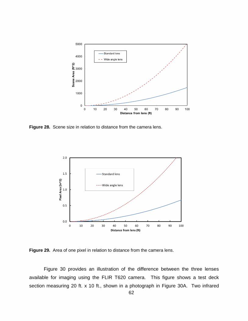
62
Figure 28. Scene size in relation to distance from the camera lens.
Figure 29. Area of one pixel in relation to distance from the camera lens.
Figure 30 provides an illustration of the difference between the three lenses
available for imaging using the FLIR T620 camera. This figure shows a test deck
section measuring 20 ft. x 10 ft., shown in a photograph in Figure 30A. Two infrared

63
markers consisting of 2 in wide foil tape in a cross pattern were placed on the deck as
spatial markers. Subsurface Styrofoam targets were cast into the deck at a depth of 2
in.. The dimensions of the Styrofoam targets were 24 in x 24 in., 18 in. x 18 in., 12 in. x
12 in. and 6 in. x 6 in.. All images in the figure were captured from a distance of 25 ft.
Figure 30B shows a thermal image of the test deck captured with a wide angle lens,
Figure 30C shows the thermal image captured with a standard lens and Figure 30D
shows a thermal image captured with a telephoto lens. The data in these figures
provide a practical illustration of the effect of using different lenses from a uniform
distance from the target.
Figure 30. Images of a concrete test deck showing photograph (A) and thermal images
captured using B) wide angle, C) standard and D) telephoto lenses.
Modeling 5.3
This section of the report focuses on finite element modeling completed to
evaluate the environmental effects on thermal contrasts for a subsurface damage in
concrete. The objective of the study was to develop a numerical model that could be

64
used to support practical inspections with a focus on the effects of the environmental
conditions surrounding the inspection. Such a model can be utilized to assess
subsurface damage with different thermal characteristics, such as different thickness of
voids or different materials within the void. For example, given a particular day’s
weather conditions and the anticipated depth of a delamination, the model could predict
if the delamination could be detected by a common thermal camera. Alternatively, such
a model could be used in post-test analysis of data to estimate the depth of a
delamination, given the known weather patterns surrounding the test and the measured
thermal contrast detected.
The model was also used to predict the thermal contrast if a void was filled with
water, which could occur following rainfall, or if the void was filled with epoxy as a repair
strategy. The model was also used to evaluate the effects of an asphalt overlay on the
thermal contrast developed from subsurface damage in the underlying concrete. This
section of the report describes an FEM model developed and tested using actual,
measured weather conditions surrounding an actual concrete block testing during
Phase I of the research. Given the academic nature of the numerical modeling, SI
units (°C) were used for modeling input and output. SI units have been maintained
herein for this portion of the research, because all calculations were completed using
these units. It is noted for the reader that to convert thermal contrast from SI units (°C)
to English (°F), simply multiply by the ratio of ⁄ , i.e. 1°C ~2°F.
Numerical Model 5.3.1
The numerical model, developed using the finite element method in COMSOL,
was based on a transient thermal energy balance between the concrete block and the
surrounding environment. The heat transfer mechanisms that occur at the concrete
surface-atmospheric boundary include radiant heating from the sun, forced and natural
convection, and emitted infrared radiation from the concrete surface. The internal heat
transfer mechanism (i.e. conduction) occurs in the concrete itself [19]. General
relationships describing these heat transfer mechanisms are available in the literature
supporting the project [20].
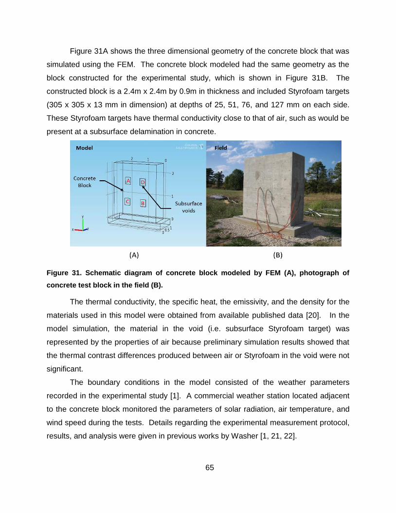
65
Figure 31A shows the three dimensional geometry of the concrete block that was
simulated using the FEM. The concrete block modeled had the same geometry as the
block constructed for the experimental study, which is shown in Figure 31B. The
constructed block is a 2.4m x 2.4m by 0.9m in thickness and included Styrofoam targets
(305 x 305 x 13 mm in dimension) at depths of 25, 51, 76, and 127 mm on each side.
These Styrofoam targets have thermal conductivity close to that of air, such as would be
present at a subsurface delamination in concrete.
Figure 31. Schematic diagram of concrete block modeled by FEM (A), photograph of
concrete test block in the field (B).
The thermal conductivity, the specific heat, the emissivity, and the density for the
materials used in this model were obtained from available published data [20]. In the
model simulation, the material in the void (i.e. subsurface Styrofoam target) was
represented by the properties of air because preliminary simulation results showed that
the thermal contrast differences produced between air or Styrofoam in the void were not
significant.
The boundary conditions in the model consisted of the weather parameters
recorded in the experimental study [1]. A commercial weather station located adjacent
to the concrete block monitored the parameters of solar radiation, air temperature, and
wind speed during the tests. Details regarding the experimental measurement protocol,
results, and analysis were given in previous works by Washer [1, 21, 22].

66
Figure 32 shows a single day of data as an example of the input data used to
model the boundary conditions of the block. The data shown in the figure shows the
solar radiation (Fig. 32A), variation of ambient temperature (Fig. 32B), and wind speed
(Fig. 32C). The time period shown in the figures is midnight to midnight (0:00 hrs). In
the experimental study, data on weather conditions and thermal images of the block
were recorded at 10 minute time intervals; this interval was used at the time-step in the
FEM. Consequently, data from the FEM and the experimental date could be compared
directly for each 10 minute time interval.
Figure 32. Environmental parameters as boundary condition in simulation on November
5, 2007: (A) solar radiation; (B) ambient temperature; and (C) wind speed.
A three month period (89 days) on the south side of the block, which was
exposed to direct solar loading from the sun, was modeled. A three month period (92

67
days) on the north side of the concrete block, which was in the shade, was also
modeled. The model was simulated separately for each month that data was collected
during the phase I research.
Simulation Results 5.3.2
Simulation results of the numerical modeling, including thermal image, surface
temperature and thermal contrast, are presented below.
5.3.2.1 Thermal Images
Figure 33A displays an example of typical thermal images obtained from the
model for the south face of the block and the actual image data collected in the
experimental test (Figure 33B). The data inputs for solar radiation, ambient temperature
change and wind speed are shown in Figure 32 for this particular day. Figure 33A
shows the surface temperature distribution obtained from the model at 12:00 p.m., and
Figure 33B shows the actual thermal image collected at that time during experimental
testing. In the figure, variations in surface temperature are represented on a color scale
applied over a temperature span of 7⁰C. Figure 33C shows the surface temperature
distribution obtained from the model at 8:00 p.m. (20:00 hours) of the same day, and
Figure 33D shows the actual thermal image at that time from the experimental test. At
this time, the target areas are cooler than the surrounding, intact concrete. As shown in
the figures, the surface temperature distributions obtained from the model closely
represent the data collected in the thermal images obtained using an infrared camera
during the experimental test completed during phase I of the research.
The variation of temperature contrast with the depth of the target can also be
observed in Figure 34, as well as the transient changes in the thermal contrast at each
target location. A positive thermal contrast is obtained when solar loading from the sun
is present (12:00 p.m.), and the negative thermal contrast is observed when solar
loading is removed and ambient temperatures are cooling (8:00 p.m., see Figure 33).
This figure illustrates the utility of the model for analytically predicting the thermal
images that would be obtained in the field using an IR camera, using actual weather
conditions (solar loading, ambient temperature variations and wind speed) as inputs for
the model. It should be noted that the images shown here are a subset of the data

68
resulting from the simulation; in the modeling, the entire month was modeled for
producing such images for each 10 minute time interval throughout the month. The
following section describes the quantitative results from the model in more detail.
Figure 33. Typical thermal images of the thermal behavior for the South side of the
concrete block: (A) the model result at noon; (B) the field test result at noon; (C) the
model result at 8:00 p.m.; and (D) the field test result at 8:00 p.m.
5.3.2.2 Surface Temperatures and Thermal Contrasts
In this section, an example of the modeled surface temperatures and resulting
thermal contrasts are presented. Figure 34 presents these data for the south and the
north faces of the block. Figure 34A shows that between the hours of 0:00 and ~8:00,
the surface temperature of the deepest target (127 mm) is the greatest and the
shallowest target (25 mm) is the lowest temperature. In the following time period, ~8:00
to ~16:00, the situation is reversed, with the 25 mm deep target having a greater
surface temperature. Similar behavior is observed from the north side modeling results,

69
shown in Figure 34B. The significant difference between the observed behaviors is the
increased change in magnitude observed for the south side that results from the radiant
heating of the sun; for the north side, only convective heat transfer from the
environment is occurring, and as a result, the change is surface temperature, over the
course of the day, is less pronounced.
Figure 34. FEM model results for the north and south sides of the test block, showing
typical results for surface temperature (A and B) and thermal contrasts (C and D)
The surface temperatures shown in Fig. 34 A and B were used to calculate the
time-varying thermal contrast for each of the subsurface voids, and these data are
shown in Figures 34C and D for the south and north sides of the block, respectively.
The thermal contrast data were processed using a 1-hour moving average to filter short-
term transient spikes in the thermal contrast data. The moving average of thermal
contrast data (solid lines) and the raw data (dash lines) are shown in the figure. As can

70
be seen in the figure, these transient spikes are primarily in the south side data, and
result from short-term effects such as a cloud moving in front of the sun or a short
period of sunshine on an otherwise cloudy day.
For the south face (Fig. 34C), the thermal contrast for each of the targets starts
to increase at different times of the day, with deeper targets developing thermal contrast
later in the day. Also, the maximum thermal contrast is decreased as the target depth
increases, as would be expected. The maximum thermal contrast for 25, 51, 76, and
127 mm deep targets at the day was approximately 7⁰C, 4⁰C, 2⁰C, and 1⁰C,
respectively. The north face (Fig. 34D) has a lower thermal contrast value for each
target, and these contrasts are more consistent over the course of the day, as shown in
the figure. The maximum thermal contrast for target depth of 25, 51, and 76 mm was
approximately 3 ⁰C, 2 ⁰C, and 1 ⁰C, respectively. For the 127 mm deep target, the
maximum thermal contrast was minimal due to the depth of the target. The data from
this model support results from the field testing conducted as part of the research
indicating the deep delaminations (> 75 mm from the surface) are difficult to image
using hand-held infrared thermography.
Figure 35 shows two weeks of the thermal contrast data for the 51 mm deep
target as an example of the comparison between model-predicted and field-measured
results for the south side of the block. It can be observed that the curve patterns of the
thermal contrast results from the model are in reasonably good agreement with the field
experiment; that is, the overall trend of the model-predicted data is consistent with the
field-measured data, generally, over the course of 14 days. Figure 35B shows an
example of the comparison between model-predicted and field-measured thermal
contrast for the 51 mm deep target for the north side of the block. In this case, there
appears to be less agreement between the model and experimental test results.

71
Figure 35. Thermal contrast determined from the numerical model and measured in the
field for A) solar loaded conditions and B) shady conditions.
Examining all the datasets of the south (sunny) side together, the thermal
contrast correlations between model results and field observed for 51 mm and 76 mm
targets are 0.92 and 0.89, respectively. Those values indicate high correlations between
model and experimental results. When the north (shaded) side was examined, the
correlation coefficients are 0.70 for both 51 mm and 76 mm targets. It can be noted that
the model correlates better in the sunny side compared to the shaded side. The
absence of solar radiation in the shaded side is likely responsible for the lower
correlation, since this provides a strong driving force for thermal contrast on the south

72
side of the block. On the north (shaded) side, convective heat transfer results in much
lower magnitude contrasts and the correlation between the model and the experimental
results is decreased. Additional information regarding the correlation of the model
results with the experimental field results can be found in the literature, including
detailed error analysis [20].
Based on the correlation analysis, it was concluded that the model was
sufficiently accurate to provide a useful tool for estimating the thermal contrasts
resulting from subsurface voids in the concrete, and provide a tool to support practical
thermal inspections. The model could also be used to predict the behavior of
subsurface voids of different characteristics, such as different thickness of a
delamination, or different materials such as a water or epoxy filling the void. The
following section of the report describes these analyses.
Parametric Studies. 5.4
Previous research had been completed examining the relationship between the
depth of a void (i.e. delamination) and the thermal contrast. Typically, a more shallow
delamination will result in larger thermal contrasts than deeper delaminations [23] [24].
Maser investigated the effects of variable delamination thickness under a certain set of
environmental variables using a simple model. A 2-dimensional, layered model was
analyzed using FEM to assess the effect of varying delamination and thickness. In this
model, the delamination was modeled as a layer of material between layers of concrete,
with appropriate thermal properties assigned to each layer in the model. The results
revealed that the thickness of the delamination affected the size of the temperature
difference (i.e. thermal contrast). Increasing the delamination thickness by a factor of
five increased the maximum thermal contrast by a factor of four [3]. The depth of the
delamination was also shown to have a significant effect on the thermal contrast
developed, with deeper delaminations showing less thermal contrast than more shallow
delaminations for the same set of environmental conditions. Based on these previous
research results, the model developed through the research was used to develop
relationships between the void depth, void thickness, and the resulting thermal contrast
under a given set of environmental conditions.

73
In addition, the model assessed the effect of having materials other than air filling
the subsurface delamination. Air-filled void is the most commonly postulated model as
a material contained in subsurface delamination. However, in field applications, the
material which fills a delamination is not necessarily air; a delamination may be filled
with water or ice, or it could be filled with epoxy which had been injected as part of a
preservation activity. Water-filled voids would be expected under saturated concrete
conditions and ice may be present if the ambient temperature drops below freezing [25].
These materials of air, water, ice, and epoxy contained in the void have different
thermal conductivity, heat capacity, and density in comparison to the sound concrete.
Among these properties, thermal conductivity is a main property affecting temperature
contrast between the void area and the sound area. Since the thermal conductivity of
air is considerably lower than that of concrete, the significant temperature differences
between a thin delaminated area and the thicker sound concrete can be expected when
the material contained in the void is air. On the other hand, since the thermal
conductivity of water is not significantly lower than that of concrete, clear thermal
differences at water filled voids would not be expected under steady state condition
However, for transient conditions, thermal contrast can be produced because of the
different heat capacities of water and concrete [25]. Maser and Roddis also studied the
effect of a water-filled delamination, finding that the presence of water greatly
diminished the thermal contrast developed for a simulated delamination 38 mm (1.5
inches) deep in the concrete [3].
Model 5.4.1
In order to conduct the numerical parametric study efficiently, a smaller block
was modeled. The same modeling parameters were used as described previously; the
model was simply reduced in geometric size for efficiency, as shown in Figure 36. The
basic geometry consisted of a concrete block 2.4 m wide by 2.4 m tall and 0.9 m deep
with a square void inserted. For parametric study of the effect of void depth and
thickness, the thermal properties of air were used to describe the voided area. The
thermal properties of water, ice, epoxy, and Styrofoam were used to study the effect of
different materials within the void.

74
Figure 36. The basic geometry of the concrete model (geometry view in COMSOL)
Three days of weather data were obtained from the experimental study (the
South/sunny side) and simulated as boundary conditions. The solar radiation (Fig.
37A), the ambient temperature (Fig. 37B), and the wind speed (Fig. 37C) were applied
in the model. Solar radiation was applied only on the top surface of the concrete block.
Convective heat transfer was simulated at the top and bottom surface of the concrete.
The four other surfaces were treated as adiabatic. All simulations were run using 10
minutes time step over a period of three consecutive days to allow the simulated block
to attain typical thermal inertia for transient heat flow. Results of the final 24 hours in
the last day were used for the analysis of results.

75
Figure 37. Three consecutive days of environmental parameters as a boundary condition in
simulation: (A) solar radiation; (B) ambient temperature; and (C) wind speed
5.4.1.1 Effect of varying void depths and void thicknesses
The first parametric study involved a basic model of a concrete block with an
embedded air void; this air void simulated the effect of subsurface delaminations at
different depths and of different thicknesses. The results of the simulation provided the
transient thermal images for the concrete surface. For quantitative analysis, surface
temperatures as a function of time from a point above the void (Tvoid) and a reference
point where there is no void (Tsound concrete) were compared and these surface
temperature differences (i.e. thermal contrast) were calculated.
Figure 38A illustrates an example of the effect of varying void depths on the
thermal contrast produced by an air-filled void (for 13 mm void thickness). The results

76
indicate that increasing depth of void reduces the thermal contrast, as would be
anticipated. The shallow void develops a greater maximum thermal contrast than a
deep void; this maximum contrast is developed more rapidly for the shallow void.
The thickness of the air-filled void was also found to affect the thermal contrast
as shown in Figure 38B (for 51 mm deep void). As shown in the figure, the greater the
thickness of the void, the larger the maximum thermal contrast was developed.
Figure 38. The time varying thermal contrast: (A) as a function of void depth, and (B) as a
function of void thickness
Figure 39A and Figure 39B present the results of the maximum thermal contrast
from voids at various depths and thicknesses, respectively. The results show some
interesting details regarding the effect of void depth and void thickness on the thermal
contrast. The maximum thermal contrast decreased nonlinearly for increasing void
depths (Fig. 39A). For example, for a void thickness of 2 mm, the maximum thermal
contrast for 25, 51, 76 and 127 mm deep void was 4.86°, 2.82°, 1.69°, and 0.69°C,
respectively. The overall behavior revealed in this figure is also of interest; as the depth
of a delamination increased, the effect of the delamination thickness decreased. In
other words, for a shallow delamination, the effect of the delamination thickness has a
large impact on the thermal contrast measured at the surface using a thermal camera.

77
In addition, Fig. 39B shows that a larger void thickness results in greater thermal
contrast. For example, in the case of 51 mm deep void, the maximum thermal contrast
increased from 1.24°C to 5.29°C with increasing thickness from 0.5 mm to 15 mm. The
overall behavior illustrated in this figure shows the greater impact of delamination
thickness as the thickness tends toward zero. In other words, the effect of thickness is
greatest when the delamination is relatively thin; as the delamination thickness
increases, the impact of that thickness decreases. This is shown in the slopes of the
curve in Figure 39B; at thickness above 4 mm, the slope of the curve tends toward zero;
at thicknesses less than 4 mm, the slope is increased, and those increases are greatest
when the depth of the delamination is small.
Figure 39 shows that the variation of the maximum thermal contrast with void
depths could be fitted by the exponential function, and the variation of the maximum
thermal contrast with void thickness could be fitted by the logarithm functions (inversion
of the exponential functions). To develop a means of resolving the thickness and depth
of a delamination, or to predict the thermal contrast, equations were developed to
express these relationships as a function of the thermal contrast and the depth and
thickness of a delamination. Although these equations included constants which were
derived based on the specific weather condition modeled here, they illustrate the
general form of equations describing the behavior and demonstrate how the FEM can
be used to develop relations that could assist in practical applications of the technology.
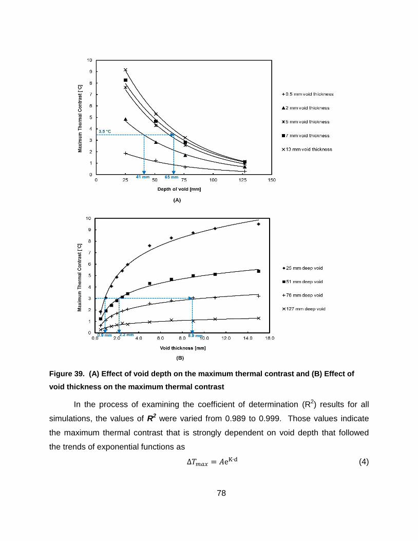
78
Figure 39. (A) Effect of void depth on the maximum thermal contrast and (B) Effect of
void thickness on the maximum thermal contrast
In the process of examining the coefficient of determination (R2) results for all
simulations, the values of R2 were varied from 0.989 to 0.999. Those values indicate
the maximum thermal contrast that is strongly dependent on void depth that followed
the trends of exponential functions as
(4)

79
where ΔTmax is the maximum thermal contrast in °C, d is the depth of void in mm, e is
the natural exponential base (e ~2.71828), A and K are constants. Equation (4) was
fitted to the maximum thermal contrast-void depth data for varying of void thicknesses
(z) from 0.5 mm to 13 mm. The best-fit exponential function was obtained by an
iterative least-square (maximum likelihood) method using Excel program.
Based on the exponential expressions obtained in this case, the relationship
between the maximum thermal contrast (ΔTmax), void depth (d), and void thickness (z)
could be expressed:
(5)
where ΔTmax in °C and both of d and z in mm. For example, the maximum thermal
contrast was computed using Equation (5) for three different thicknesses: 0.5 mm, 2
mm, and 7 mm, which represent a thin void, a typical void thickness, and a thick void,
respectively. Table 4 presents the results of the calculations. Again, it should be noted
that the use of Equation (5) for predicting the maximum thermal contrast was proper for
the model under a particular set of weather conditions.
TABLE 4. Example of estimation of maximum thermal contrast
Void thickness, z [mm] A = 3.852 ln(z)+5.294 Maximum thermal contrast [°C]
0.5 2.624 ΔTmax= 2.624 ᵡ 0.980d
2 7.964 ΔTmax= 7.964 ᵡ 0.980d
7 12.790 ΔTmax=12.790 ᵡ 0.980d
3.1.1. Estimation depth of void
Inversion of Equation (5) allows the estimation of the depth of void, given the
known weather patterns surrounding the test, the measured thermal contrast detected
during the test, and the anticipated thickness of a delamination.
The depth of void could be determined either mathematically or graphically. It
could be obtained mathematically from the following equation
[
] (6)
where ΔTmax is the maximum thermal contrast in ˚C.

80
The data shown in Figure 39A provides a simple procedure to estimate the depth
of void graphically. For example, for a 3.5˚C maximum thermal contrast (highlighted as
the blue dash lines), the estimated void depth was approximately 41 mm when the void
thickness was 2 mm. It was predicted as 65 mm when the void thickness was 7 mm.
The model could also be used to evaluate the capability and limitation of
detectable void. For example, it could estimate the minimum thickness of detectable
void either mathematically or graphically, when the expected maximum thermal contrast
and the anticipated depth of a void were given.
The data shown in Fig. 39B illustrates a simple procedure to estimate the
minimum thickness of detectable void graphically. For example, in the case of a 3˚C
thermal contrast threshold (highlighted as the blue dash lines), the minimum thickness
of detectable void was approximately 0.9, 2.2, and 8.9 mm when void depth was 25, 51,
and 76 mm deep void, respectively. If the void depth were 127 mm, the thermal
contrast of 3˚C would not be developed, given the weather condition modeled.
The significance of these results are as follows:
1. Both the thickness of the subsurface void and depth of the subsurface void
effect the thermal contrast developed at the surface.
2. The effect of the void thickness is more pronounced for shallow void than for
deeper voids.
3. FEM modeling using actual weather conditions can provide a practical tool for
analyzing the results of thermographic testing to estimate the depth or
thickness of a delamination.
It should be noted, in regard to item (3), that either the depth of the void, or the
thickness of the void, must be estimated to obtain a unique result. It should also be
noted that the modeling results have been summarized herein to illustrate important
results. Readers can review more detailed descriptions of the modelling process and
results in the referenced literature.
Effect of Asphalt Overlays 5.4.2
The thermal model was applied to the case of concrete with an asphalt overlay to
investigate the effect of varying asphalt thickness on the thermal contrast produced by

81
an air filled void. A model of the concrete block with a varying asphalt thickness from 40
mm to 120 mm was used to predict thermal contrast under the weather conditions as
shown in Figure 37. The thermal properties of air were used to describe the voided
area. The depths of the voids were 51 mm and 76 mm from the front surface of the
block, and the thickness of the void was 13 mm in the simulations.
Figure 40 shows the time varying thermal contrast as a function of the asphalt
thickness. The results show that the presence of the asphalt overlay in the model
reduced the thermal contrast significantly and was a function of asphalt thickness.
Figure 40. The time varying thermal contrast as a function of asphalt thickness: (A) 51
mm deep void (B) 76 mm deep void.
The relationship between the maximum thermal contrast and asphalt thickness
for 51 mm deep void and 76 mm deep void, both with 13 mm void thickness, is shown in
Figure 41. The trends of the predictions were the same as the first case (i.e. effect of
varying void depths) since the overlay was a thermal mass above the void. Thus, the
mass reduced the thermal contrast associated with the void. It can also be seen that
there was a certain condition of asphalt thickness for which the thermal contrast would
be too small (less than 0.5 °C) to be measured. This result shows the limits of
applicability of IR thermography to asphalt-overlaid concrete bridge decks. In general,
the results show that an asphalt overlay of 40 mm (~1.5 in.) reduces the thermal
contrast by approximately 50%. However, it is significant that the model shows that
although the thermal contrast will be diminished, it is not eliminated. As a result, it can

82
be concluded that although thermal contrast will be reduced as a result of an asphalt
overlay, subsurface delamination in the concrete can still be detected using infrared
thermography, particularly if the overlay thickness is less than ~ 40 mm.
Figure 41. Effect of asphalt thickness on the maximum thermal contrast.
Effect of the Materials in Delamination 5.4.3
Five different materials present in the void were modeled: air, water, ice, epoxy
and Styrofoam. The Styrofoam filled void was included in this case so that the thermal
contrasts results from the model and the experimental data could be compared. Table
2 shows the material properties for each material as well as the material properties of
the sound concrete that was used for simulation in this case study. The thickness of the
void was 13 mm for all simulations.
TABLE 5. Material properties for case 2 involving different materials contained in the
void and the sound concrete.
Material k Cp Ρ
[W/(m °C)] [J/(kg °C)] [kg/m3]
Void (air) 0.024 700 1.2
Void (Styrofoam) 0.027 1300 35
Void (water) 0.6 4200 1000
Void (ice) 2.2 2050 915
Void (epoxy) 1.24 1200 1530

83
The sound concrete 1.8 1000 2300
Figure 42 shows the time varying thermal contrast as a function of materials
present in the void for 51 mm deep void. The results showed that when the void was air
filled, the substantial difference in thermal conductivity (k) between air and concrete
(Table 2) supported expectations of significant thermal contrasts between a void area
and the sound concrete. Since the thermal conductivity of water, ice, and epoxy
adhesive was not substantially different from that of concrete, the thermal contrasts
produced from the void was significantly less pronounced.
Figure 42. The time varying thermal contrast as a function of the materials present in the void
The data shown in Figure 42 demonstrate that subsurface delamination
containing water, ice or epoxy would not be detectable using infrared thermography.
This result was verified during field verification testing when an area previously repaired
using epoxy injection was imaged using a thermal camera, and no contrast between
that area and intact concrete was found. The result indicates that the success of epoxy
injection activities could be verified using a thermal camera, because a delamination
containing epoxy would not appear as an area of thermal contrast in a thermal image. If
a delaminated area was not properly filled with epoxy, it would be expected to appear in
the thermal image.

84
Model Verification using Field Testing 5.4.4
The results of the modeling effort were verified during a field test. The objective
of the field test was to verify the effectiveness of the model for predicting the thermal
contrast of a delamination in the field. The hourly weather data, which included solar
radiation, ambient temperature, and wind speed, were obtained from a nearby weather
station where the field testing was conducted. The characteristics of the void were
obtained from the field coring test. The capability of the model was evaluated by
comparing the thermal contrasts predicted by the model, using the ambient weather
conditions at the time of the field test, and those detected by thermography inspection
during the field test.
Field testing was conducted on a pedestrian bridge over College Avenue in
Columbia, Missouri. The bridge was constructed in the early 1970s by the Missouri
Department of Transportation and Stephens College. An upgrade project to replace the
main walkway of the bridge was initiated in the summer of 2012. The deck was
constructed with ~51 mm concrete overlay, as determined by coring after the field
testing.
Thermal data was collected using the typical FLIR T620 camera used throughout
the study by participating states. This camera was used to collect images of the surface
of the bridge at one hour intervals between 6:30 a.m. and 10:30 p.m.
Figures 43A and 43B show the photograph and thermal image bridge deck at
2:30 p.m. In the thermal image, three spot temperatures (T1, T2, and Tsound concrete)
were noted as the points of interest for the study. T1 and T2 were the surface
temperatures at the locations where hammer sounding results indicated a delamination
may be present. In the area of T1, hammer sounding results were inconclusive
regarding the presence of a subsurface delamination. Corresponding thermal images
showed very small thermal contrast in this area. In the area of T2 , hammer sounding
results were confident that there was a delamination, and corresponding thermal
images showed a large thermal contrast. Tsound concrete was the surface temperature of
the concrete that was determined by sounding and thermal imaging to be intact
concrete.

85
Figure 43. The digital image and the thermal image at 2:30 p.m. (obtained from the field IR
thermography testing)
For quantitative analysis, the apparent temperature differences (i.e. thermal
contrast) between the voids and the sound concrete were calculated. The results of
thermal contrasts throughout the day are shown in Figure 43 as “field data 1” and “field
data 2.” The field data 1 was obtained from T1-Tsound concrete and the field data 2 was
obtained from T2-Tsound concrete. The maximum thermal contrasts (ΔTmax) for each area
are indicated in the last column in Table 6.
After evaluation of the thermal contrast, cores were taken at the selected
locations to confirm the existence of voids and to determine their depth and thickness.
Data of the coring test were collected for 2 locations and the results are shown in Table
6. The coring indicated that at location 1, there was not observable separation between
the concrete overlay and the concrete substrate. The overlay and substrate were in
contact, and this observation was confirmed by water retained in the hole from which
the core was extracted.
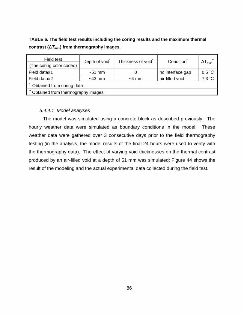
86
TABLE 6. The field test results including the coring results and the maximum thermal
contrast (ΔTmax) from thermography images.
Field test Depth of void* Thickness of void* Condition* ΔTmax
** (The coring color coded)
Field data#1 ~51 mm 0 no interface gap 0.5 ˚C
Field data#2 ~43 mm ~4 mm air-filled void 7.3 ˚C * Obtained from coring data ** Obtained from thermography images
5.4.4.1 Model analyses
The model was simulated using a concrete block as described previously. The
hourly weather data were simulated as boundary conditions in the model. These
weather data were gathered over 3 consecutive days prior to the field thermography
testing (in the analysis, the model results of the final 24 hours were used to verify with
the thermography data). The effect of varying void thicknesses on the thermal contrast
produced by an air-filled void at a depth of 51 mm was simulated; Figure 44 shows the
result of the modeling and the actual experimental data collected during the field test.

87
Figure 44. Thermal contrast as a function of void thickness for 51 mm deep void
For the model verification, the maximum thermal contrasts predicted by the
model and using equation 3, and those obtained from the field test using IR
themography, were compared. The predicted maximum thermal contrasts were
computed using the void thickness and the void depth data obtained from the coring
test. For example, for a 43 mm void depth and a 4 mm void thickness (field data #2 in
Table 6), the predicted maximum thermal contrast by the model was approximately
7.9˚C, while the measured maximum thermal contrast detected by the field
thermography testing was 7.3˚C (Table 6). The result of the post-test model analysis
shows that the model could predict the maximum thermal contrast of subsurface voids
in concrete under a given set of environmental conditions surrounding the test as well
as the anticipated depth and thickness of a delamination.
Discussion of Numerical Modeling Results 5.4.5
This portion of the report focuses on the evaluation of the effect of key
parameters expected to influence the detectability of the subsurface voids, such as void

88
depth, void thickness, and material in the void. Two cases of analysis were performed
using finite element analysis: (1) the effect of varying void depths and void thickness
and (2) the effect of different materials contained in the void. In addition, a simplified
prediction of void depth from the measured thermal contrast and a simplified estimation
of minimum thickness of detectable void were developed mathematically and
graphically.
The findings from the study demonstrated that the maximum thermal contrasts
were a function of both the depth of the void and the thickness of the void. The
maximum thermal contrast decreased exponentially by a constant multiple of 0.98 as
the void depth increased. The maximum thermal contrast increased nonlinearly (as a
logarithm function) with increasing thickness of the void. The results also showed that
changes in maximum thermal contrast were more pronounced for voids located closer
to the surface. The study led to a simple procedure for estimating the depth of a void as
a function of the thickness of the void and the thermal contrast. The results from the
study of the effect of different materials contained in a subsurface void (i.e.
delamination) demonstrated that air-filled voids produced a significant thermal contrast
compared to water-filled voids, ice-filled voids, and epoxy adhesive-filled voids. The
differences of the thermal contrast for each material in the voided areas arose from
different thermal behavior due to different properties of heat conduction and/or specific
heat compared to the thermal properties of the sound concrete.
An example of post-test model analysis was presented that compared the model
prediction of thermal contrast with the actual measured thermal contrast. The model
was created for the specific set of weather conditions and the void depth and thickness
obtained from the coring test. It was found that the model result was sufficiently
accurate to predict the maximum thermal contrast when compared with the measured
using an infrared camera.
Based on the results of these studies, it was concluded that the developed model
provided valuable information on the expected responses and possible limitations of
using thermographic techniques to detect subsurface voids (i.e. delaminations) in
concrete bridge components.

89
6 CONCLUSIONS
This study has evaluated the implementation of infrared thermography for the
condition assessment of highway bridges. This evaluation has included training and
field testing across 12 states participating in the study. Each of these states was
provided an infrared camera for testing within their respective bridge inspection and
evaluation programs. Training was provided on the use and application of the
technology, and verification testing was conducted in most of the participating states.
Additional verification testing is ongoing.
Tools to support the implementation of infrared thermography included a web-
based BIP that provided users with real-time weather conditions, recommendation for
inspection, and future weather conditions for planning purposes. A web-based SDS
database documenting state experience with infrared thermography was developed,
with entries from various participants, and experiences from the training sessions and
verification testing.
Laboratory testing was completed that examined the wind speed guidance
included in the Guidelines and developed guidance on the appropriate use of various
lenses that may be used on the thermal cameras used in the research. A numerical
model was also developed to provide a tool for analyzing infrared thermography test
results. This numerical model was used to analyze the effect of asphalt overlays, the
depth and thickness of subsurface damage, and the effect of different materials
contained within a subsurface defect. This numerical model was validated based on
prior research, and demonstrated in a verification test.
The objectives of the research were as follows
Quantify the capability and reliability of thermal imaging technology in the field
Field test and validate inspection guidelines for the application of thermal imaging
for bridge inspection
Identify and overcome implementation barriers
The capability and reliability was demonstrated through field testing of the
technology and comparison with a secondary inspection technique, typically hammer
sounding but including coring and drilling into the bridge deck. In terms of quantifying
the capability and reliability of the technology, conclusions based on the data available

90
(to date) from the implementation study and verification study indicated that the
technology was reliable when implemented within the constraints of the guidelines, if the
depth of the delamination was 3 inches or less. Field verification studies and state
experience showed that when the depth of the delamination is greater than 3 inches,
the damage may not be detected using the inspection conditions described in the
guidelines. A model developed during the research also demonstrated that the
thickness of the subsurface delamination played a significant role in the detectability of
the damage. Using the model to analyze a field testing of a bridge deck with an overlay,
it was shown that a debonded overlay without separation of the substrate produced
thermal contrast of < 1° C, making it difficult to detect in the field.
Overall, the verification testing and results reported through the implementation
study showed that the Guidelines provided suitable conditions for detection of
subsurface damage in concrete. Participants reported a high degree of confidence in
results when damage was detected. There was one field verification experience where
thermal contrast was not detected in the field for an area where hammer sounding
indicated that there was a delamination. Solar loading over a portion of a substructure,
which introduces high thermal gradient across the surface of the concrete, was also
found to limit the effectiveness of infrared thermography.
Additional research is needed to analyze, collectively, the results of the
verification study and results reported from participants in the SDS; this research is
ongoing. This analysis is aimed at better quantifying test results from the study.
The primary implementation barrier identified during the study was a lack of
available resources. It is significant that anticipated barriers, such as difficulty using the
technology or interpreting results, were not found during the course of the study. For
most participants, the technology worked effectively for the purposes intended. Several
participants indicated that the technology is being integrated into condition assessment
programs for the purpose of scoping renovation activities and to focus inspection efforts
where most needed. This result was not unanimous; one participant did not find the
technology useful for detection of delaminations in bridge decks.

91
Guideline Revisions 6.1
As part of the research, several revisions to the Guidelines were made.
Generally, these revisions consisted of additions to the Guidelines. The three most
significant changes are summarized as follows
Wind Speed Guidance: Values for acceptable wind speeds were modified
to correlate with data provided by the NWS. This change was made to
simplify the use of the Guidelines, since these data are more readily
available
Inspection Time Window: A figure was added to the Guidelines to make it
possible to adjust the inspection time windows indicated in the Guidelines
according to the length of the day, which changes throughout the year.
Guidance on Use of Lenses: Additional guidance was included to provide
information regarding the appropriate lens to use as a function of distance.
Additional changes to the Guidelines were editorial in nature.
Ongoing and Future Research 6.2
Ongoing research from the study includes experimental testing of new
technologies developed during the course of the research. This includes a new
technology, called Infrared Ultra Time Domain (IR-UTD), which uses time-lapse infrared
images to analyze the presence of subsurface damage. This technology overcomes
several limitations of hand-held infrared thermography. The technology does not
require optimized weather conditions to detect subsurface damage, and is capable of
imaging damage at depths greater than 3 in. A second technology that features a
thermal camera mounted on a vehicle is also being tested. This technology, known as
the Infrared Deck and Soffit Scanner, is unique from existing technologies because it is
capable of being mounted on any vehicle with a trailer hitch; also, it is configured to
capture images of both bridge decks and deck soffit areas of overpass bridges. The
technology is also unique because it provides high precision, spatially-reference thermal
images that can be easily interpreted and has a high accuracy. In addition, the
technology can provide quantitative data on the area (in square feet) of both bridge

92
decks and deck soffit areas. Results of field testing of these technologies will be
reported in Volume II of this report.

93
REFERENCES
1. Washer, G., R.G. Fenwick, and N.K. Bolleni, Development of Hand-held Thermographic Inspection Technologies. 2009, MoDOT: MoDOT: Missouri Department of Transportation, Jefferson City, MO. p. 124. 2. Bertolini, L., et al., Corrosion of Steel in Concrete. 1 ed. 2004: Wiley-VCH. 392. 3. Maser, K.R. and W.M.K. Roddis, Principles of thermography and radar for bridge deck assessment. Journal of Transportation Engineering, 1990. 116(5): p. 583-601. 4. Russell, H.G., NCHRP Synthesis 333: Concrete Bridge Deck Performance, N.C.H.R. Program, Editor. 2004, Transportation Research Board: Washington, D.C. p. 188. 5. Ghorbanpoor, A. and N. Benish, Non-Destructive Testing of Wisconsin Highway Bridges. 2003, The Wisconsin Department of Transportation: Milwaukee, Wisconsin. p. 108. 6. Rens, K.L., C.L. Nogueira, and D.J. Transue, Bridge management and nondestructive evaluation. Journal of performance of constructed facilities, 2005. 19: p. 3-16. 7. Roddis, W.M.K., Concrete bridge deck assessment using thermography and radar, in Civil Engineering. 1987, Massachusetts Institute of Technology: Massachusetts. 8. Moore, M.E., et al., Reliability of Visual Inspection of Highway Bridges, FHWA, Editor. 2001, USDOT: Washington, DC. p. 516. 9. Scott, M., et al., A comparison of nondestructive evaluation methods for bridge deck assessment. NDT & E Int., 2003. 36(4): p. 245-255. 10. Olson, L.D., Y. Tinkey, and P. Miller. Concrete Bridge Condition Assessment with Impact Echo Scanning. in GeoHunan 2011 Emerging Technologies for Material, Design, Rehabilitation, and Inspection of Roadway Pavements. 2011. Hunan, China: ASCE. 11. Maierhofer, C., Nondestructive Evaluation of Concrete Infrastructure with Ground Penetrating Radar. J. Mater. Civ. Eng., 2003. 15(3): p. 287-297. 12. Parrillo, R., A. Haggan, and R. Roberts, Bridge Deck Condition Assessment using Ground Penetrating Radar, in 9th European NDT Conference (ECNDT). 2006: Berlin, GR. 13. Clemena, G.G. and W.T. McKeel Jr, The Applicability of Infrared Thermography in the Detection of Delamination in Bridge Decks 1977, Virginia Highway and Transportation Research Council: Virginia. 14. Weil, G.J., Infrared Thermographic Techniques, in CRC Handbook on Nondestructive Testing of Concrete, M. V.M. and N.J. Carino, Editors. 1991, CRC Press: Boca Raton, FL. p. 305-316. 15. Manning, D.G. and F.B. Holt, Detecting delaminations in concrete bridge decks. Concr. Int., 1980. 2(11): p. 34-41. 16. Manning, D.G. and F.B. Holt, The development of deck assessment by radar and thermography. 1986. p. 13-20. 17. ASTM, D4788-03: Standard test method for detecting delaminations in bridge decks using infrared thermography. 2007: West Conshohocken, PA. 18. Washer, G., et al., Guidelines for thermographic inspection of concrete bridge components in shaded conditions. Transportation Research Record, 2013(2360): p. 13-20. 19. Branco, F.A. and P.A. Mendes, Thermal actions for concrete bridge design. Journal of Structural Engineering, 1993. 119(8): p. 2313-2331. 20. Rumbayan, R., Modeling Of Environmental Effects On Thermal Detection Of Subsurface Damage For Concrete Bridges, in Department of Civil and Environmental Engineering 2013, University of Missouri: Columbia, MO. p. 225.

94
21. Washer, G., et al., Effects of Environmental Variables on Infrared Imaging of Subsurface Features of Concrete Bridges. Transportation Research Record: Journal of the Transportation Research Board, 2009. 2108: p. 107-114. 22. Washer, G., R.G. Fenwick, and N.K. Bolleni, Effects of Solar Loading on Infrared Imaging of Subsurface Features in Concrete. Journal of Bridge Engineering 2010. 15(4): p. 384-390. 23. Manning, D.G., Detecting Defects and Deterioration in Highway Structures, in Tech. Report NCHRP Synthesis 118. 1985, National Cooperative Highway Research Program (NCHRP), Transportation Research Board, National Research Council, Washington, D.C. 24. Manning, D.G. and F.B. Holt, Detecting Delaminations in Concrete Bridge Decks. Concrete International, 1980. 2: p. 34-41. 25. Roddis, W.M.K., Concrete Bridge Deck Assessment using Thermography and Radar, in Civil Engineering. 1987, Massachusetts Institute of Technology.