Fiducial Generalized Confidence Interval for Median Lethal ...
24
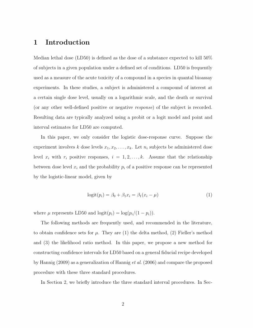
Fiducial Generalized Confidence Interval for Median Lethal Dose (LD50) ∗ Lidong E † , Jan Hannig ‡ and Hari Iyer § July 20, 2009 Abstract Median lethal dose (LD50) is a common measure of acute toxicity of a com- pound in a species. In this paper we propose a new method for constructing confidence intervals for LD50 for a logistic-response curve. Our approach is based on Hannig (2009) who developed an extension of R. A. Fisher’s fiducial argument and provided a general recipe for interval estimation that is applica- ble in virtually any situation. The method uses Gibbs sampling to empirically estimate the percentiles of the fiducial distribution for LD50. The resulting in- tervals are compared with three other competing confidence interval procedures – the Delta method interval, Fieller intervals, and Likelihood Ratio intervals. Simulation results show that fiducial intervals have a satisfactory overall per- formance and are more stable than the competing methods in terms of coverage probability. Furthermore, we establish the asymptotic correctness of the cov- erage probability of fiducial intervals. The median of the generalized fiducial distributions also appears to give unbiased point estimates of LD50. Keywords: median lethal dose (LD50), Fiducial Generalized Confidence In- terval (FGCI), Gibbs sampling. ∗ This work was supported in part by the National Science Foundation under Grant 0707037. † Department of Statistics, Colorado State University ‡ Department of Statistics and Operation Research, The University of North Carolina at Chapel Hill, e-mail: [email protected] § Department of Statistics, Colorado State University, Fort Collins, Colorado, 80523; and Cater- pillar Inc., 100 NE Adams St, Peoria, Illinois, 61629, e-mail: [email protected] 1
Transcript of Fiducial Generalized Confidence Interval for Median Lethal ...
Fiducial Generalized Confidence Interval for Median
Lethal Dose (LD50) ∗
Lidong E†, Jan Hannig‡and Hari Iyer§
July 20, 2009
Abstract
Median lethal dose (LD50) is a common measure of acute toxicity of a com-
pound in a species. In this paper we propose a new method for constructing
confidence intervals for LD50 for a logistic-response curve. Our approach is
based on Hannig (2009) who developed an extension of R. A. Fisher’s fiducial
argument and provided a general recipe for interval estimation that is applica-
ble in virtually any situation. The method uses Gibbs sampling to empirically
estimate the percentiles of the fiducial distribution for LD50. The resulting in-
tervals are compared with three other competing confidence interval procedures
– the Delta method interval, Fieller intervals, and Likelihood Ratio intervals.
Simulation results show that fiducial intervals have a satisfactory overall per-
formance and are more stable than the competing methods in terms of coverage
probability. Furthermore, we establish the asymptotic correctness of the cov-
erage probability of fiducial intervals. The median of the generalized fiducial
distributions also appears to give unbiased point estimates of LD50.
Keywords: median lethal dose (LD50), Fiducial Generalized Confidence In-
terval (FGCI), Gibbs sampling.
∗This work was supported in part by the National Science Foundation under Grant 0707037.†Department of Statistics, Colorado State University‡Department of Statistics and Operation Research, The University of North Carolina at Chapel
Hill, e-mail: [email protected]§Department of Statistics, Colorado State University, Fort Collins, Colorado, 80523; and Cater-
pillar Inc., 100 NE Adams St, Peoria, Illinois, 61629, e-mail: [email protected]
1
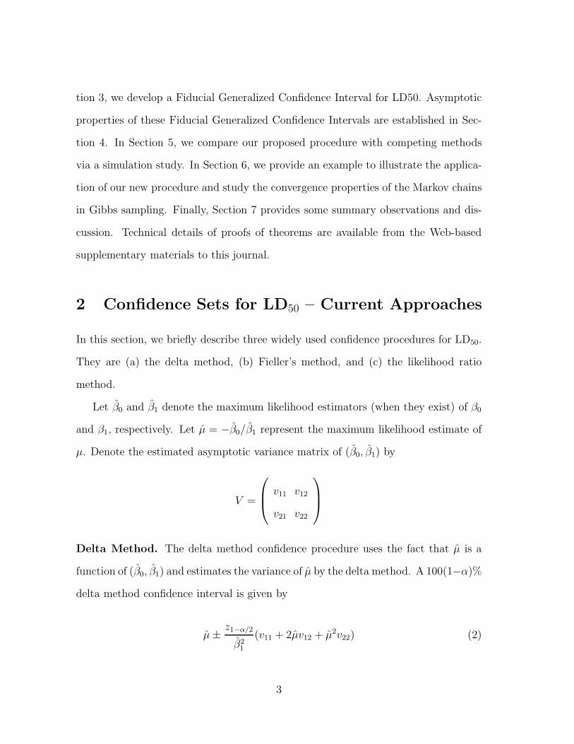
1 Introduction
Median lethal dose (LD50) is defined as the dose of a substance expected to kill 50%
of subjects in a given population under a defined set of conditions. LD50 is frequently
used as a measure of the acute toxicity of a compound in a species in quantal bioassay
experiments. In these studies, a subject is administered a compound of interest at
a certain single dose level, usually on a logarithmic scale, and the death or survival
(or any other well-defined positive or negative response) of the subject is recorded.
Resulting data are typically analyzed using a probit or a logit model and point and
interval estimates for LD50 are computed.
In this paper, we only consider the logistic dose-response curve. Suppose the
experiment involves k dose levels x1, x2, . . . , xk. Let ni subjects be administered dose
level xi with ri positive responses, i = 1, 2, . . . , k. Assume that the relationship
between dose level xi and the probability pi of a positive response can be represented
by the logistic-linear model, given by
logit(pi) = β0 + β1xi = β1(xi − µ) (1)
where µ represents LD50 and logit(pi) = log(pi/(1 − pi)).
The following methods are frequently used, and recommended in the literature,
to obtain confidence sets for µ. They are (1) the delta method, (2) Fieller’s method
and (3) the likelihood ratio method. In this paper, we propose a new method for
constructing confidence intervals for LD50 based on a general fiducial recipe developed
by Hannig (2009) as a generalization of Hannig et al. (2006) and compare the proposed
procedure with these three standard procedures.
In Section 2, we briefly introduce the three standard interval procedures. In Sec-
2
tion 3, we develop a Fiducial Generalized Confidence Interval for LD50. Asymptotic
properties of these Fiducial Generalized Confidence Intervals are established in Sec-
tion 4. In Section 5, we compare our proposed procedure with competing methods
via a simulation study. In Section 6, we provide an example to illustrate the applica-
tion of our new procedure and study the convergence properties of the Markov chains
in Gibbs sampling. Finally, Section 7 provides some summary observations and dis-
cussion. Technical details of proofs of theorems are available from the Web-based
supplementary materials to this journal.
2 Confidence Sets for LD50 – Current Approaches
In this section, we briefly describe three widely used confidence procedures for LD50.
They are (a) the delta method, (b) Fieller’s method, and (c) the likelihood ratio
method.
Let β̂0 and β̂1 denote the maximum likelihood estimators (when they exist) of β0
and β1, respectively. Let µ̂ = −β̂0/β̂1 represent the maximum likelihood estimate of
µ. Denote the estimated asymptotic variance matrix of (β̂0, β̂1) by
V =
⎛⎜⎝ v11 v12
v21 v22
⎞⎟⎠
Delta Method. The delta method confidence procedure uses the fact that µ̂ is a
function of (β̂0, β̂1) and estimates the variance of µ̂ by the delta method. A 100(1−α)%
delta method confidence interval is given by
µ̂ ± z1−α/2
β̂21
(v11 + 2µ̂v12 + µ̂2v22) (2)
3
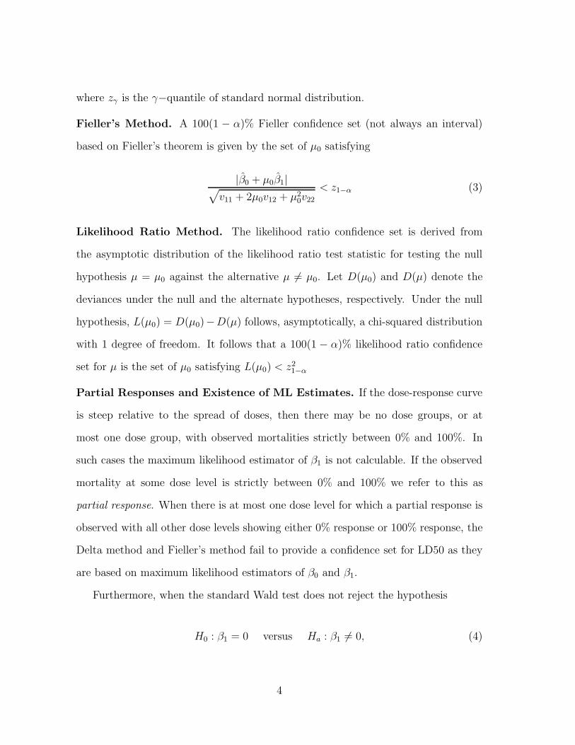
where zγ is the γ−quantile of standard normal distribution.
Fieller’s Method. A 100(1 − α)% Fieller confidence set (not always an interval)
based on Fieller’s theorem is given by the set of µ0 satisfying
|β̂0 + µ0β̂1|√v11 + 2µ0v12 + µ2
0v22
< z1−α (3)
Likelihood Ratio Method. The likelihood ratio confidence set is derived from
the asymptotic distribution of the likelihood ratio test statistic for testing the null
hypothesis µ = µ0 against the alternative µ �= µ0. Let D(µ0) and D(µ) denote the
deviances under the null and the alternate hypotheses, respectively. Under the null
hypothesis, L(µ0) = D(µ0)−D(µ) follows, asymptotically, a chi-squared distribution
with 1 degree of freedom. It follows that a 100(1 − α)% likelihood ratio confidence
set for µ is the set of µ0 satisfying L(µ0) < z21−α
Partial Responses and Existence of ML Estimates. If the dose-response curve
is steep relative to the spread of doses, then there may be no dose groups, or at
most one dose group, with observed mortalities strictly between 0% and 100%. In
such cases the maximum likelihood estimator of β1 is not calculable. If the observed
mortality at some dose level is strictly between 0% and 100% we refer to this as
partial response. When there is at most one dose level for which a partial response is
observed with all other dose levels showing either 0% response or 100% response, the
Delta method and Fieller’s method fail to provide a confidence set for LD50 as they
are based on maximum likelihood estimators of β0 and β1.
Furthermore, when the standard Wald test does not reject the hypothesis
H0 : β1 = 0 versus Ha : β1 �= 0, (4)
4
Fieller’s confidence sets are either the entire real line or unions of disjoint intervals.
Likewise, if the hypothesis (4) could not be rejected by the likelihood ratio test, the
likelihood ratio confidence sets are either the entire real line or unions of disjoint
intervals. Sitter and Wu (1993) argue that making inference about µ in such cases
is unreasonable since the regression relationship is not significant at level α. They
suggest, instead, to either reassess the meaning of the LD50 or collect more data at
other dose levels. Persuaded by the point of view in Sitter and Wu (1993), these cases
are excluded from the analysis of simulation results in many studies, for example in
Harris et al. (1999) and in Huang et al. (2002a). However when we are dealing with
small experiments, we might not have enough information to reject β1 = 0 although
β1 is not equal to zero. In recognition of these facts, we propose a fiducial solution
which provides a finite confidence interval in any situation and, at the same time,
maintains the coverage probability at acceptable levels.
3 A Fiducial Confidence Interval for LD50
In this section we develop a new procedure for constructing confidence intervals for
µ based on its generalized fiducial distribution.
Generalized Fiducial Distributions. We first review the definition of a generalized
fiducial distribution from Hannig et al. (2006) as generalized by Hannig (2009). Let
Y be a random vector with a distribution indexed by a (possibly vector) parameter
ξ ∈ Ξ. Hannig (2009) defines a generalized fiducial distribution for ξ as follows.
Assume that Y has a structural representation given by
Y = G(U, ξ),
5
where U is a random variable or random vector whose distribution is fully known and
free of unknown parameters, and G is a jointly measurable function of U and ξ. After
observing y as the value of Y we define Q(y, u) as a set-valued function
Q(y, u) = {ξ : y = G(u, ξ)}.
The set {ξ : y = G(u, ξ)} may be empty, may consist of a single element, or, as will
be the case in this paper, may consist of more than one element. In the case Q(y, u)
contains more than one element we select one of the elements in Q(y, u) according to
some, possibly random, rule. Mathematically this is achieved as follows: assume for
any measurable set S, there is a random element V (S) with support S, where S is
the closure of S. We then use the function V (Q(y, u)) in our definition. The function
V (Q(y, u)) may be viewed as a generalized inverse of the function G. Here G defines
u as an implicit function of ξ and y is regarded as fixed. Following Hannig (2009) we
define a generalized fiducial distribution of ξ as a conditional distribution of
V (Q(y, U∗)) given {Q(y, U∗) �= ∅}. (5)
Here U∗ is an independent copy of U . An alternative approach, in cases where Q(y, u)
may contain more than one element, would be to use the Dempster-Shafer calculus
(Dempster, 2008) and work with set valued objects to derive corresponding confidence
procedures.
Generalized Fiducial Inference for LD50. We now apply the above recipe to
the LD50 problem. Set antilogit(x) = ex/(1 + ex). First we describe the structural
equation in our problem.
Let Yij, i = 1, . . . , k, j = 1, . . . , ni denote the jth subject’s response to the dose
6
level xi. Clearly Yij follows a Bernoulli distribution with success probability pi =
antilogit(β0 + β1xi). Thus we can model
Yij = I(0,antilogit(β0+β1xi))(Uij), j = 1, . . . , ni, i = 1, . . . , k. (6)
Here (β0, β1) are unknown parameters and Uij are independent standard uniform
random variables. Denote U i = (Ui1, . . . , Uini), i = 1, . . . , k, Si =
∑ni
j=1 Yij, and
Y i = (Yi1, . . . , Yini), i = 1, . . . , k. Then we have Si ∼Binomial(ni, pi).
We now derive the generalized fiducial distribution of LD50. This derivation closely
follows the derivation of a generalized fiducial distribution for binomial distribution
in Hannig (2009). Define the mapping Qi(yi, ui) : [0, 1]ni → [0, 1], i = 1, . . . , k, as
follows
Qi(yi, ui) =
⎧⎪⎪⎪⎪⎪⎪⎪⎪⎪⎪⎪⎪⎪⎪⎨⎪⎪⎪⎪⎪⎪⎪⎪⎪⎪⎪⎪⎪⎪⎩
[0, ui,1:ni] if si = 0
(ui,ni:ni, 1] if si = ni
(ui,si:ni, ui,si+1:ni
] if si = 1, . . . , ni − 1 and
∑ni
j=1 I(yij = 1)I(uij ≤ ui,si:ni) = si
∅ otherwise,
where yi, si and ui are realizations of Y i, Si and U i respectively, i = 1, . . . , k, and
Ui,si:nidenotes the sth
i order statistic among Ui1, . . . , Uini.
If there was no link between the pi values for the various doses, we would be
dealing with k independent binomial distributions with unrelated parameters and
the generalized fiducial distribution of pi would have been the conditional distri-
bution of Qi(yi, U�i ) conditional on the event Qi(yi, U
�i ) �= ∅. By exchangeability
this conditional distribution is the same as the distribution of the random inter-
7
val (U�i,si:ni
, U�i,si+1:ni
), c.f., Hannig (2009). Here we set U�i,0:ni
= 0 and U�i,ni+1:ni
= 1.
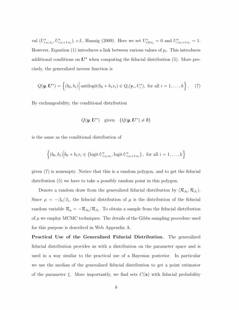
However, Equation (1) introduces a link between various values of pi. This introduces
additional conditions on U � when computing the fiducial distribution (5). More pre-
cisely, the generalized inverse function is
Q(y, U �) ={
(b0, b1)∣∣∣ antilogit(b0 + b1xi) ∈ Qi(yi, U
�i ), for all i = 1, . . . , k
}. (7)
By exchangeability, the conditional distribution
Q(y, U �) given {Q(y, U �) �= ∅}
is the same as the conditional distribution of
{(b0, b1)
∣∣∣b0 + b1xi ∈(logit U�
i,si:ni, logitU�
i,si+1:ni
), for all i = 1, . . . , k
}
given (7) is nonempty. Notice that this is a random polygon, and to get the fiducial
distribution (5) we have to take a possibly random point in this polygon.
Denote a random draw from the generalized fiducial distribution by (Rβ0,Rβ1).
Since µ = −β0/β1, the fiducial distribution of µ is the distribution of the fiducial
random variable Rµ = −Rβ0/Rβ1. To obtain a sample from the fiducial distribution
of µ we employ MCMC techniques. The details of the Gibbs sampling procedure used
for this purpose is described in Web Appendix A.
Practical Use of the Generalized Fiducial Distribution. The generalized
fiducial distribution provides us with a distribution on the parameter space and is
used in a way similar to the practical use of a Bayesian posterior. In particular
we use the median of the generalized fiducial distribution to get a point estimator
of the parameter ξ. More importantly, we find sets C(x) with fiducial probability
8
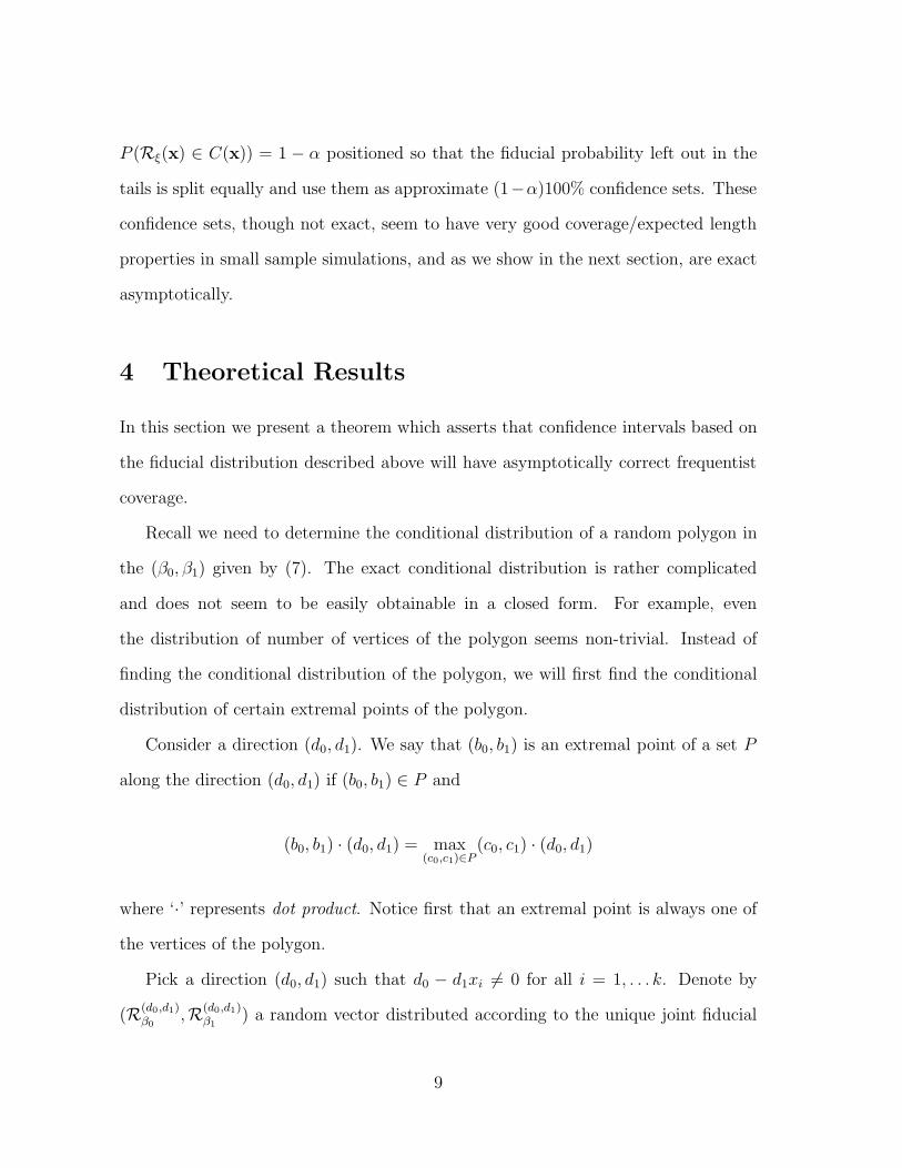
P (Rξ(x) ∈ C(x)) = 1 − α positioned so that the fiducial probability left out in the
tails is split equally and use them as approximate (1−α)100% confidence sets. These
confidence sets, though not exact, seem to have very good coverage/expected length
properties in small sample simulations, and as we show in the next section, are exact
asymptotically.
4 Theoretical Results
In this section we present a theorem which asserts that confidence intervals based on
the fiducial distribution described above will have asymptotically correct frequentist
coverage.
Recall we need to determine the conditional distribution of a random polygon in
the (β0, β1) given by (7). The exact conditional distribution is rather complicated
and does not seem to be easily obtainable in a closed form. For example, even
the distribution of number of vertices of the polygon seems non-trivial. Instead of
finding the conditional distribution of the polygon, we will first find the conditional
distribution of certain extremal points of the polygon.
Consider a direction (d0, d1). We say that (b0, b1) is an extremal point of a set P
along the direction (d0, d1) if (b0, b1) ∈ P and
(b0, b1) · (d0, d1) = max(c0,c1)∈P
(c0, c1) · (d0, d1)
where ‘·’ represents dot product. Notice first that an extremal point is always one of
the vertices of the polygon.
Pick a direction (d0, d1) such that d0 − d1xi �= 0 for all i = 1, . . . k. Denote by
(R(d0,d1)β0
,R(d0,d1)β1
) a random vector distributed according to the unique joint fiducial
9
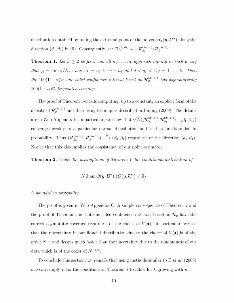
distribution obtained by taking the extremal point of the polygon Q(y, U�) along the
direction (d0, d1) in (5). Consequently, set R(d0,d1)µ = −R(d0,d1)
β0/R(d0,d1)
β1.
Theorem 1. Let k ≥ 2 be fixed and all n1, . . . , nk approach infinity in such a way
that qj = lim nj/N , where N = n1 + · · · + nk and 0 < qj < 1, j = 1, . . . , k. Then
the 100(1 − α)% one sided confidence interval based on R(d0,d1)µ has asymptotically
100(1 − α)% frequentist coverage.
The proof of Theorem 1 entails computing, up to a constant, an explicit form of the
density of R(d0,d1)µ and then using techniques described in Hannig (2009). The details
are in Web Appendix B. In particular, we show that√
N((R(d0,d1)β0
,R(d0,d1)β1
)−(β1, β1))
converges weakly to a particular normal distribution and is therefore bounded in
probability. Thus (R(d0,d1)β0
,R(d0,d1)β1
)P−→ (β0, β1) regardless of the direction (d0, d1).
Notice that this also implies the consistency of our point estimator.
Theorem 2. Under the assumptions of Theorem 1, the conditional distribution of
N diam Q(y, U �)|{Q(y, U�) �= ∅}
is bounded in probability.
The proof is given in Web Appendix C. A simple consequence of Theorem 2 and
the proof of Theorem 1 is that one sided confidence intervals based on Rµ have the
correct asymptotic coverage regardless of the choice of V (•). In particular, we see
that the uncertainty in our fiducial distribution due to the choice of V (•) is of the
order N−1 and decays much faster than the uncertainty due to the randomness of our
data which is of the order of N−1/2.
To conclude this section, we remark that using methods similar to E et al. (2008)
one can simply relax the conditions of Theorem 1 to allow for k growing with n.
10
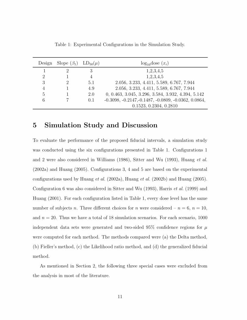
Table 1: Experimental Configurations in the Simulation Study.
Design Slope (β1) LD50(µ) log10dose (xi)
1 2 3 1,2,3,4,52 1 4 1,2,3,4,53 2 5.1 2.056, 3.233, 4.411, 5.589, 6.767, 7.9444 1 4.9 2.056, 3.233, 4.411, 5.589, 6.767, 7.9445 1 2.0 0, 0.463, 3.045, 3.296, 3.584, 3.932, 4.394, 5.1426 7 0.1 -0.3098, -0.2147,-0.1487, -0.0809, -0.0362, 0.0864,
0.1523, 0.2304, 0.2810
5 Simulation Study and Discussion
To evaluate the performance of the proposed fiducial intervals, a simulation study
was conducted using the six configurations presented in Table 1. Configurations 1
and 2 were also considered in Williams (1986), Sitter and Wu (1993), Huang et al.
(2002a) and Huang (2005). Configurations 3, 4 and 5 are based on the experimental
configurations used by Huang et al. (2002a), Huang et al. (2002b) and Huang (2005).
Configuration 6 was also considered in Sitter and Wu (1993), Harris et al. (1999) and
Huang (2001). For each configuration listed in Table 1, every dose level has the same
number of subjects n. Three different choices for n were considered – n = 6, n = 10,
and n = 20. Thus we have a total of 18 simulation scenarios. For each scenario, 1000
independent data sets were generated and two-sided 95% confidence regions for µ
were computed for each method. The methods compared were (a) the Delta method,
(b) Fieller’s method, (c) the Likelihood ratio method, and (d) the generalized fiducial
method.
As mentioned in Section 2, the following three special cases were excluded from
the analysis in most of the literature.
11
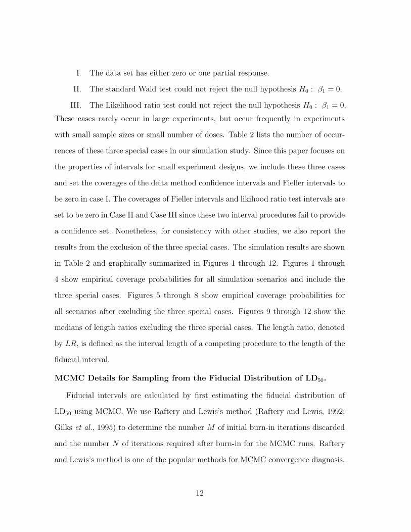
I. The data set has either zero or one partial response.
II. The standard Wald test could not reject the null hypothesis H0 : β1 = 0.
III. The Likelihood ratio test could not reject the null hypothesis H0 : β1 = 0.
These cases rarely occur in large experiments, but occur frequently in experiments
with small sample sizes or small number of doses. Table 2 lists the number of occur-
rences of these three special cases in our simulation study. Since this paper focuses on
the properties of intervals for small experiment designs, we include these three cases
and set the coverages of the delta method confidence intervals and Fieller intervals to
be zero in case I. The coverages of Fieller intervals and likihood ratio test intervals are
set to be zero in Case II and Case III since these two interval procedures fail to provide
a confidence set. Nonetheless, for consistency with other studies, we also report the
results from the exclusion of the three special cases. The simulation results are shown
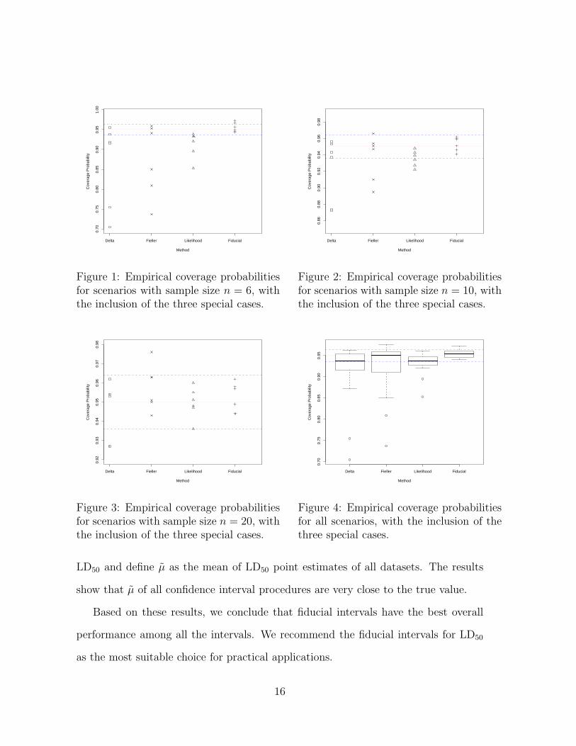
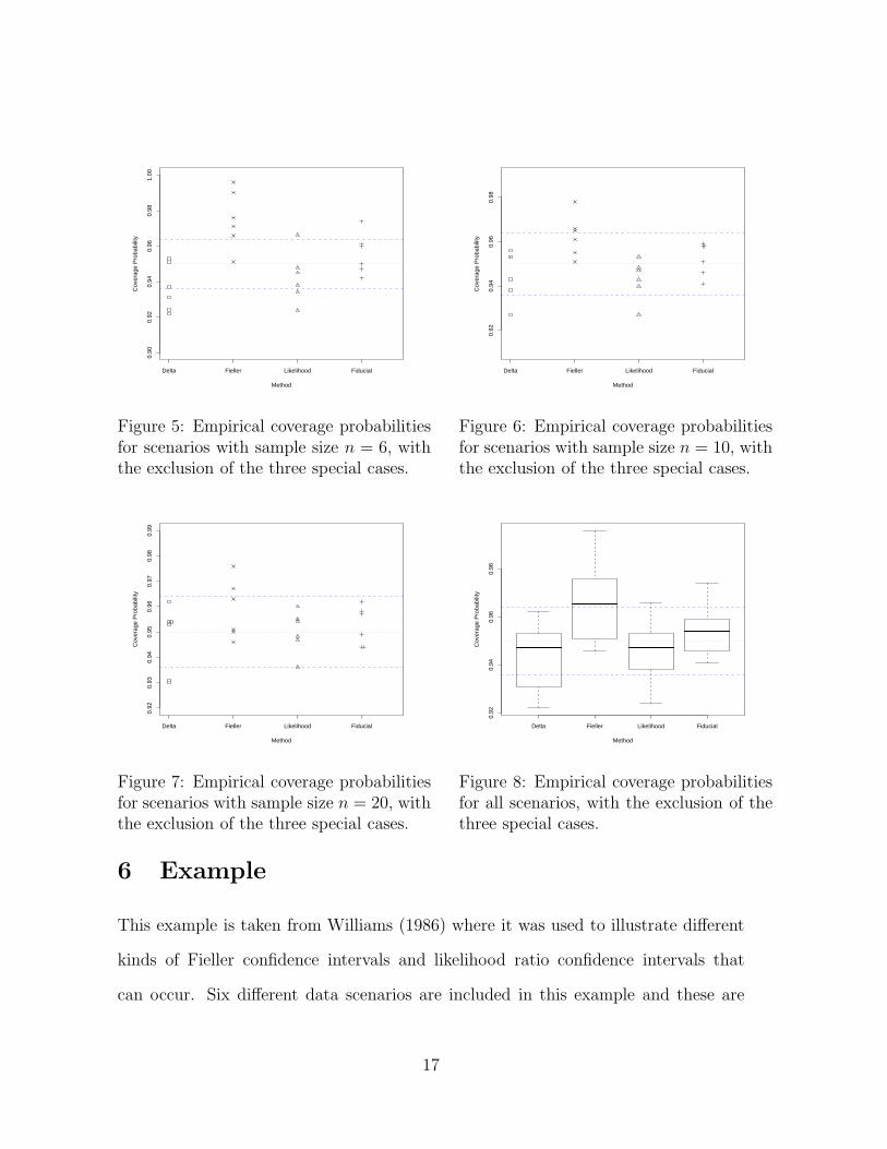
in Table 2 and graphically summarized in Figures 1 through 12. Figures 1 through
4 show empirical coverage probabilities for all simulation scenarios and include the
three special cases. Figures 5 through 8 show empirical coverage probabilities for
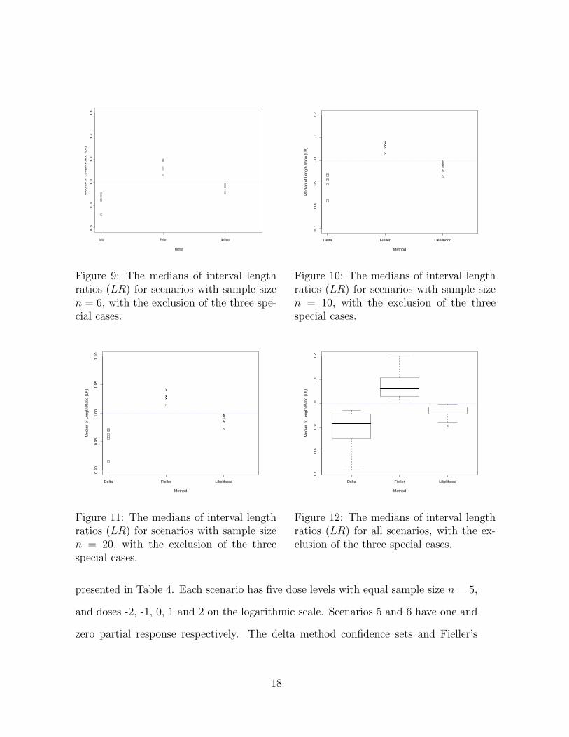
all scenarios after excluding the three special cases. Figures 9 through 12 show the
medians of length ratios excluding the three special cases. The length ratio, denoted
by LR, is defined as the interval length of a competing procedure to the length of the
fiducial interval.
MCMC Details for Sampling from the Fiducial Distribution of LD50.
Fiducial intervals are calculated by first estimating the fiducial distribution of
LD50 using MCMC. We use Raftery and Lewis’s method (Raftery and Lewis, 1992;
Gilks et al., 1995) to determine the number M of initial burn-in iterations discarded
and the number N of iterations required after burn-in for the MCMC runs. Raftery
and Lewis’s method is one of the popular methods for MCMC convergence diagnosis.
12
It is intended to calculate the number of iterations necessary to estimate some quantile
of interest within an acceptable of accuracy, at a specified probability level, from a
single run of a Markov chain. We implement this method using the Raftery and
Lewis’s diagnostic function in CODA package (Plummer et al., 2006). The inputs are
the quantile q to be estimated, the desired accuracy r, the required probability s of
attaining the specified accuracy and a convergence tolerance ε. Here we are interested
in two-sided 95% confidence intervals corresponding to q = 0.025 and 0.975. We select
r = 0.005, s = 0.95 and ε = 0.001. Brooks and Roberts (1999) examined Raftery and
Lewis’s convergence diagnosis method and showed that this method might lead to an
underestimate of the true burn-in length. To avoid this problem, we set M = 1000
if the value of M suggested by Raftery and Lewis’s method is less than 1000. The
largest value of M and N obtained for each combination of parameters (β0, β1, µ)
and quantiles (0.025, 0.975) are used as the burn-in length and number of iterations
required after burn-in, respectively. The M +N iterations are run and the diagnostics
process is repeated to check if iterations are sufficient.
One concern with the MCMC method is how to sample the output of a stationary
Markov chain. A systemic subsample of the chain, using only every kth observation,
is one of the popular methods and it produces approximately iid draws. Geyer (1992)
and MacEachern and Berliner (1994) argued convincingly against the use of subsam-
pling by proving that the estimator resulting from subsampling has larger variance
and is poorer than the non-subsampled estimator. They suggest using the entire
Markov chain, instead of subsampling. Based on their argument, we use the entire
Markov chain in our study.
Simulation Results. The results show that the three competing confidence intervals
are very liberal for scenarios with small sample sizes when we include all three special
13
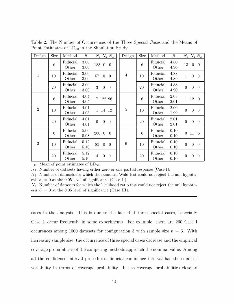
Table 2: The Number of Occurrences of the Three Special Cases and the Means ofPoint Estimates of LD50 in the Simulation Study.
Design Size Method µ̃ N1 N2 N3
1
6Fiducial 3.00
183 0 0Other 3.00
10Fiducial 3.00
57 0 0Other 3.00
20Fiducial 3.00
3 0 0Other 3.00
2
6Fiducial 4.04
7 122 96Other 4.05
10Fiducial 4.01
1 14 12Other 4.03
20Fiducial 4.01
0 0 0Other 4.01
3
6Fiducial 5.00
260 0 0Other 5.08
10Fiducial 5.12
85 0 0Other 5.10
20Fiducial 5.12
4 0 0Other 5.10
Design Size Method µ̃ N1 N2 N3
4
6Fiducial 4.80
13 0 0Other 4.90
10Fiducial 4.88
1 0 0Other 4.89
20Fiducial 4.88
0 0 0Other 4.90
5
6Fiducial 2.03
1 12 0Other 2.01
10Fiducial 2.00
0 0 0Other 1.99
20Fiducial 2.01
0 0 0Other 2.01
6
6Fiducial 0.10
0 11 6Other 0.10
10Fiducial 0.10
0 0 0Other 0.10
20Fiducial 0.10
0 0 0Other 0.10
µ̃: Mean of point estimates of LD50.N1: Number of datasets having either zero or one partial response (Case I).N2: Number of datasets for which the standard Wald test could not reject the null hypoth-esis β1 = 0 at the 0.05 level of significance (Case II).N3: Number of datasets for which the likelihood ratio test could not reject the null hypoth-esis β1 = 0 at the 0.05 level of significance (Case III).
cases in the analysis. This is due to the fact that three special cases, especially
Case I, occur frequently in some experiments. For example, there are 260 Case I
occurences among 1000 datasets for configuration 3 with sample size n = 6. With
increasing sample size, the occurrence of three special cases decrease and the empirical
coverage probabilities of the competing methods approach the nominal value. Among
all the confidence interval procedures, fiducial confidence interval has the smallest
variability in terms of coverage probability. It has coverage probabilities close to
14
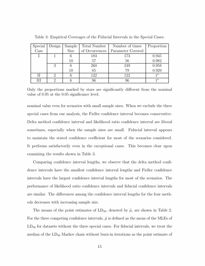
Table 3: Empirical Coverages of the Fiducial Intervals in the Special Cases.
Special Design Sample Total Number Number of times ProportionCase Size of Occurrences Parameter Covered
I 1 6 183 173 0.94510 57 56 0.982
3 6 260 249 0.95810 85 79 0.929
II 2 6 122 122 1�
III 2 6 96 96 1�
Only the proportions marked by stars are significantly different from the nominalvalue of 0.95 at the 0.05 significance level.
nominal value even for scenarios with small sample sizes. When we exclude the three
special cases from our analysis, the Fieller confidence interval becomes conservative.
Delta method confidence interval and likelihood ratio confidence interval are liberal
sometimes, especially when the sample sizes are small. Fiducial interval appears
to maintain the stated confidence coefficient for most of the scenarios considered.
It performs satisfactorily even in the exceptional cases. This becomes clear upon
examining the results shown in Table 3.
Comparing confidence interval lengths, we observe that the delta method confi-
dence intervals have the smallest confidence interval lengths and Fieller confidence
intervals have the largest confidence interval lengths for most of the scenarios. The
performance of likelihood ratio confidence intervals and fiducial confidence intervals
are similar. The differences among the confidence interval lengths for the four meth-
ods decreases with increasing sample size.
The means of the point estimates of LD50, denoted by µ̃, are shown in Table 2.
For the three competing confidence intervals, µ̃ is defined as the mean of the MLEs of
LD50 for datasets without the three special cases. For fiducial intervals, we treat the
median of the LD50 Markov chain without burn-in iterations as the point estimate of
15
Delta Fieller Likelihood Fiducial
0.70
0.75
0.80
0.85
0.90
0.95
1.00
Method
Cov
erag
e P
roba
bilit
y
Figure 1: Empirical coverage probabilitiesfor scenarios with sample size n = 6, withthe inclusion of the three special cases.
Delta Fieller Likelihood Fiducial
0.86
0.88
0.90
0.92
0.94
0.96
0.98
Method
Cov
erag
e P
roba
bilit
y
Figure 2: Empirical coverage probabilitiesfor scenarios with sample size n = 10, withthe inclusion of the three special cases.
Delta Fieller Likelihood Fiducial
0.92
0.93
0.94
0.95
0.96
0.97
0.98
Method
Cov
erag
e P
roba
bilit
y
Figure 3: Empirical coverage probabilitiesfor scenarios with sample size n = 20, withthe inclusion of the three special cases.
Delta Fieller Likelihood Fiducial
0.70
0.75
0.80
0.85
0.90
0.95
Method
Cov
erag
e P
roba
bilit
y
Figure 4: Empirical coverage probabilitiesfor all scenarios, with the inclusion of thethree special cases.
LD50 and define µ̃ as the mean of LD50 point estimates of all datasets. The results
show that µ̃ of all confidence interval procedures are very close to the true value.
Based on these results, we conclude that fiducial intervals have the best overall
performance among all the intervals. We recommend the fiducial intervals for LD50
as the most suitable choice for practical applications.
16
Delta Fieller Likelihood Fiducial
0.90
0.92
0.94
0.96
0.98
1.00
Method
Cov
erag
e P
roba
bilit
y
Figure 5: Empirical coverage probabilitiesfor scenarios with sample size n = 6, withthe exclusion of the three special cases.
Delta Fieller Likelihood Fiducial
0.92
0.94
0.96
0.98
Method
Cov
erag
e P
roba
bilit
y
Figure 6: Empirical coverage probabilitiesfor scenarios with sample size n = 10, withthe exclusion of the three special cases.
Delta Fieller Likelihood Fiducial
0.92
0.93
0.94
0.95
0.96
0.97
0.98
0.99
Method
Cov
erag
e P
roba
bilit
y
Figure 7: Empirical coverage probabilitiesfor scenarios with sample size n = 20, withthe exclusion of the three special cases.
Delta Fieller Likelihood Fiducial
0.92
0.94
0.96
0.98
Method
Cov
erag
e P
roba
bilit
y
Figure 8: Empirical coverage probabilitiesfor all scenarios, with the exclusion of thethree special cases.
6 Example
This example is taken from Williams (1986) where it was used to illustrate different
kinds of Fieller confidence intervals and likelihood ratio confidence intervals that
can occur. Six different data scenarios are included in this example and these are
17
Delta Fieller Likelihood
0.6
0.8
1.0
1.2
1.4
1.6
Method
Media
n o
f Length
Ratio (
LR
)
Figure 9: The medians of interval lengthratios (LR) for scenarios with sample sizen = 6, with the exclusion of the three spe-cial cases.
Delta Fieller Likelihood
0.7
0.8
0.9
1.0
1.1
1.2
Method
Med
ian
of L
engt
h R
atio
(LR
)
Figure 10: The medians of interval lengthratios (LR) for scenarios with sample sizen = 10, with the exclusion of the threespecial cases.
Delta Fieller Likelihood
0.90
0.95
1.00
1.05
1.10
Method
Med
ian
of L
engt
h R
atio
(LR
)
Figure 11: The medians of interval lengthratios (LR) for scenarios with sample sizen = 20, with the exclusion of the threespecial cases.
Delta Fieller Likelihood
0.7
0.8
0.9
1.0
1.1
1.2
Method
Med
ian
of L
engt
h R
atio
(LR
)
Figure 12: The medians of interval lengthratios (LR) for all scenarios, with the ex-clusion of the three special cases.
presented in Table 4. Each scenario has five dose levels with equal sample size n = 5,
and doses -2, -1, 0, 1 and 2 on the logarithmic scale. Scenarios 5 and 6 have one and
zero partial response respectively. The delta method confidence sets and Fieller’s
18
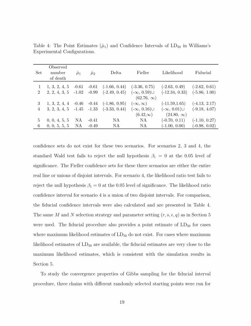
Table 4: The Point Estimates (µ̂1) and Confidence Intervals of LD50 in Williams’sExperimental Configurations.
ObservedSet number µ̂1 µ̂2 Delta Fieller Likelihood Fiducial
of death
1 1, 3, 2, 4, 5 -0.61 -0.61 (-1.66, 0.44) (-3.36, 0.75) (-2.63, 0.49) (-2.62, 0.61)2 2, 2, 4, 3, 5 -1.02 -0.99 (-2.49, 0.45) (-∞, 0.59)∪ (-12.34, 0.33) (-5.86, 1.00)
(62.76, ∞)3 1, 3, 2, 4, 4 -0.46 -0.44 (-1.86, 0.95) (-∞,∞) (-11.59,1.65) (-4.13, 2.17)4 3, 2, 3, 4, 5 -1.45 -1.33 (-3.33, 0.44) (-∞, 0.16)∪ (-∞, 0.01)∪ (-9.18, 4.07)
(6.42,∞) (24.80, ∞)5 0, 0, 4, 5, 5 NA -0.41 NA NA (-0.70, 0.11) (-1.10, 0.27)6 0, 0, 5, 5, 5 NA -0.49 NA NA (-1.00, 0.00) (-0.98, 0.02)
confidence sets do not exist for these two scenarios. For scenarios 2, 3 and 4, the
standard Wald test fails to reject the null hypothesis β1 = 0 at the 0.05 level of
significance. The Fieller confidence sets for these three scenarios are either the entire
real line or unions of disjoint intervals. For scenario 4, the likelihood ratio test fails to
reject the null hypothesis β1 = 0 at the 0.05 level of significance. The likelihood ratio
confidence interval for scenario 4 is a union of two disjoint intervals. For comparison,
the fiducial confidence intervals were also calculated and are presented in Table 4.
The same M and N selection strategy and parameter setting (r, s, ε, q) as in Section 5
were used. The fiducial procedure also provides a point estimate of LD50 for cases
where maximum likelihood estimates of LD50 do not exist. For cases where maximum
likelihood estimates of LD50 are available, the fiducial estimates are very close to the
maximum likelihood estimates, which is consistent with the simulation results in
Section 5.
To study the convergence properties of Gibbs sampling for the fiducial interval
procedure, three chains with different randomly selected starting points were run for
19
each set. Gelman and Rubin’s statistic (Gelman and Rubin, 1992) and Geweke’s
statistic (Geweke, 1992) were calculated based on the required N iterations after
burn-in and used to diagnose the convergence of the MCMC output. The general
rule of thumb is that the Gelman and Rubin’s statistic should be below 1.2 for all
parameters in order for the chain to be judged to have converged properly (Gelman
et al., 1996). Geweke’s statistic is a standard Z-score. Therefore, Geweke’s statistic
less than the 0.95 percentile of the standard normal distribution suggests conver-
gence. Table 5 summarizes the resulting Gelman and Rubin’s statistics and Geweke’s
statistics. The results show that all Gelman and Rubin’s statistics are less than 1.2
and only two among 64 Geweke’s statistics are greater than 1.96, which suggests
satisfactory convergence and complete mixture.
7 Summary Remarks
We have provided a new method for interval estimation of LD50 using data from a
dose-response study under a simple logistic regression model. The method is based
on the generalized fiducial distribution of LD50 and follows the recipe provided in
Hannig (2009). A simulation study was conducted to compare the performance of the
proposed method with three other commonly used competing methods. The results
of this study demonstrate that the fiducial interval method for LD50 has satisfactory
coverage levels whereas the competing methods could claim this only for larger sample
sizes. In fact, the fiducial intervals appear to maintain adequate coverage even in the
so called exceptional cases.
In terms of interval lengths, only the likelihood ratio intervals showed performance
comparable with the fiducial intervals but the likelihood intervals fail to maintain
coverage probabilities close to the nominal values when sample sizes are small. Addi-
20
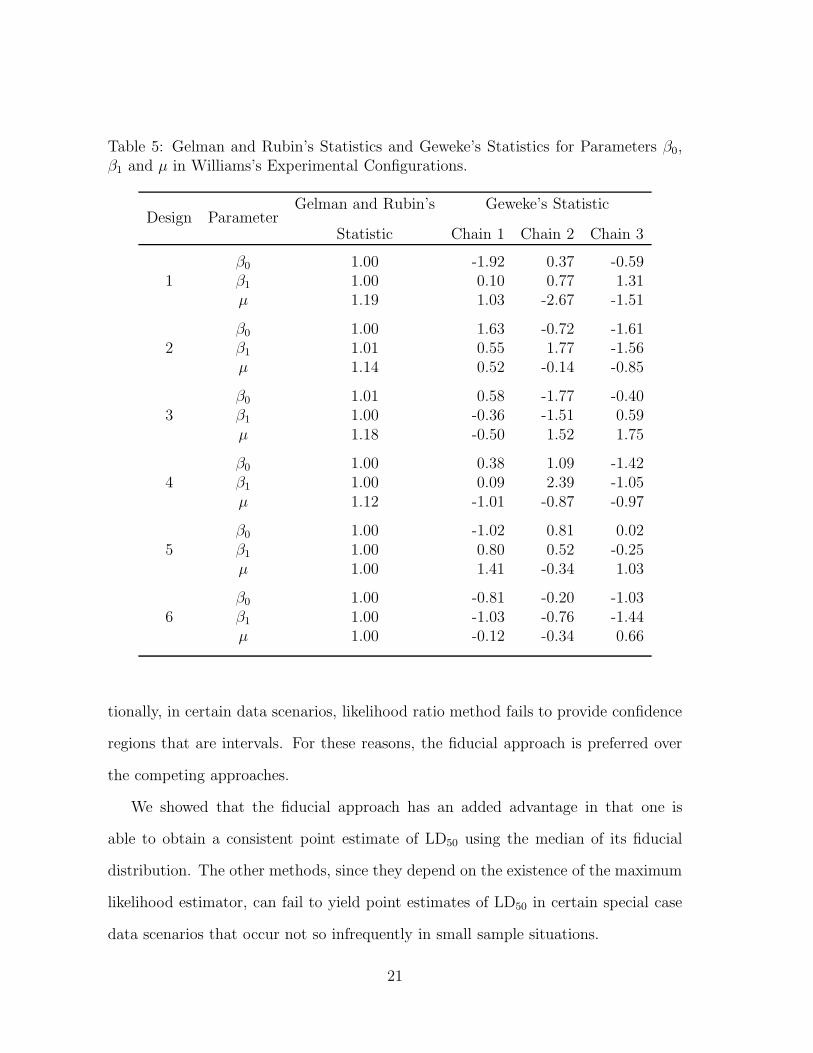
Table 5: Gelman and Rubin’s Statistics and Geweke’s Statistics for Parameters β0,β1 and µ in Williams’s Experimental Configurations.
Design ParameterGelman and Rubin’s Geweke’s Statistic
Statistic Chain 1 Chain 2 Chain 3
β0 1.00 -1.92 0.37 -0.591 β1 1.00 0.10 0.77 1.31
µ 1.19 1.03 -2.67 -1.51
β0 1.00 1.63 -0.72 -1.612 β1 1.01 0.55 1.77 -1.56
µ 1.14 0.52 -0.14 -0.85
β0 1.01 0.58 -1.77 -0.403 β1 1.00 -0.36 -1.51 0.59
µ 1.18 -0.50 1.52 1.75
β0 1.00 0.38 1.09 -1.424 β1 1.00 0.09 2.39 -1.05
µ 1.12 -1.01 -0.87 -0.97
β0 1.00 -1.02 0.81 0.025 β1 1.00 0.80 0.52 -0.25
µ 1.00 1.41 -0.34 1.03
β0 1.00 -0.81 -0.20 -1.036 β1 1.00 -1.03 -0.76 -1.44
µ 1.00 -0.12 -0.34 0.66
tionally, in certain data scenarios, likelihood ratio method fails to provide confidence
regions that are intervals. For these reasons, the fiducial approach is preferred over
the competing approaches.
We showed that the fiducial approach has an added advantage in that one is
able to obtain a consistent point estimate of LD50 using the median of its fiducial
distribution. The other methods, since they depend on the existence of the maximum
likelihood estimator, can fail to yield point estimates of LD50 in certain special case
data scenarios that occur not so infrequently in small sample situations.
21
Asymptotic properties of the fiducial interval were also studied. It was proved
that the fiducial intervals have, asymptotically, the correct frequentist coverage.
An efficient computational approach was developed, using Gibbs Sampling, for
numerical calculation of fiducial confidence intervals. The method is very efficient
and is suitable for routine application in real experiments. The conceptual extension
of the fiducial approach to higher order logistic regression models is straightforward
but the details related to computational issues need to be worked out.
References
Brooks, S. P. and Roberts, G. O. (1999) On quantile estimation and markov chain
monte carlo convergence. Biometrika, 86, 710–717.
Dempster, A. P. (2008) The Dempster-Shafer Calculus for Statisticians. International
Journal of Approximate Reasoning, 48, 365–377.
E, L., Hannig, J. and Iyer, H. K. (2008) Fiducial Intervals for Variance Components in
an Unbalanced Two-Component Normal Mixed Linear Model. Journal of American
Statistical Association, 103, 854–865.
Gelman, A., Carlin, J., Stern, H. S. and Rubin, D. B. (1996) Bayesian Data Analysis.
New York: Chapman and Hall.
Gelman, A. and Rubin, D. B. (1992) Inference from iterative simulation using multiple
sequences. Statistical Science, 7, 457–511.
Geweke, J. (1992) Evaluating the Accuracy of Sampling-Based Approaches to Calcu-
lating Posterior Moments, vol. 4. UK: Oxford.
22
Geyer, C. J. (1992) Practical markov chain monte carlo. Statistical Science, 7, 473–
483.
Gilks, W. R., Spiegelhalter, D. J. and Richardson, S. (1995) Markov Chain Monte
Carlo in Practice. London: Chapman and Hall.
Hannig, J. (2009) On generalized fiducial inference. Statistica Sinica, 19, 491–544.
Hannig, J., Iyer, H. K. and Patterson, P. (2006) Fiducial generalized confidence in-
tervals. Journal of the American Statistical Association, 101, 254–269.
Harris, P., Hann, M., Kirby, S. P. J. and Dearden, J. C. (1999) Interval estimation
of the median effective dose for a logistic dose-response curve. Journal of Applied
Statistics, 26, 715–722.
Huang, Y. (2001) Various methods of interval estimation of the median effective dose.
Communications in Statistics - Simulation, 30, 99–112.
Huang, Y. (2005) On a family of interval estimators of effective doses. Computational
Statistics and Data Analysis, 49, 131–146.
Huang, Y., Harris, P., Kirby, S. P. J. and Dearden, J. C. (2002a) Improved approaches
to interval estimation of effective doses for a logistic dose-response curve. Journal
of Statistical Computation and Simulation, 72, 565–584.
Huang, Y., Harris, P., Kirby, S. P. J. and Dearden, J. C. (2002b) A modified fieller
interval for the interval estimation of effective doses for a logistic dose-response
curve. Computational Statistics and Data Analysis, 40, 59–74.
MacEachern, S. N. and Berliner, L. M. (1994) Subsampling the gibbs sampler. The
American Statistician, 48, 188–190.
23
Plummer, P., Best, N., Cowles, K. and Vines, K. (2006) The coda package, version
0.10-7. CRAN: The Comprehensive R Network.
Raftery, A. E. and Lewis, S. M. (1992) One long run with diagnostics: Implementation
strategies for markov chain mote carlo. Statistical Science, 7, 493–497.
Sitter, R. R. and Wu, C. F. J. (1993) On the accuracy of fieller intervals for binary
response data. Journal of the American Statistical Association, 88, 1021–1025.
Williams, D. A. (1986) Interval estimation of the median lethal dose. Biometrics, 42,
641–645.
24