Fiber Pres 3

1

LIGHTWAVE

ENGINEERING

Fiber Attenuation

Dr. Abid [email protected]

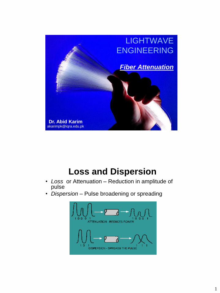
• Loss or Attenuation – Reduction in amplitude of pulse

• Dispersion – Pulse broadening or spreading

Loss and Dispersion

2

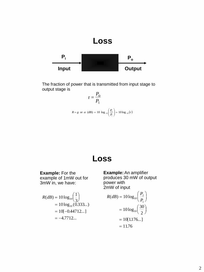
The fraction of power that is transmitted from input stage to output stage is

Input

Pi

Output

Po

Po

Pi

r =

Loss

rP

PgR

i

o log 10 log 10 (dB) or 1010

Example: For the example of 1mW out for 3mW in, we have:

R dB( ) log

10

1

310

10 0 333

10 0 44712

4 7712

10log ( . ...)

[ . ...]

. ...

Example: An amplifier produces 30 mW of output power with 2mW of input

R dBP

P( ) log

10 10

2

1

1030

2

10 1176

1176

10log

[ . ...]

.

Loss

3

Attenuation Characteristics (Theoretical)

Fiber Losses

window #1: 0.8-0.9µm

window #2: 1.25-1.35µm

windows #3: 1.5-1.6 µm

why not #4: 1.0-1.2 µm?

Rayleigh Scattering

Total Loss

Second Window

First Window

Third Window

800 900 1000 1100 1200 1300 1400 1500 1600 1700

3.0

2.5 2.0

1.5

1.0

0.5

OH Absorption Peak

Wavelength (nm)

Att

enu

ation

(d

B/k

m)

Fiber Losses

• Attenuation Characteristics (Experimental)

• Total Attenuation

Waveguide

losses

4

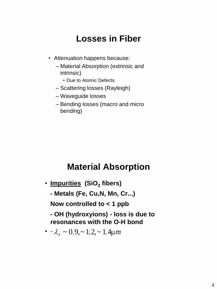
Losses in Fiber

• Attenuation happens because:

– Material Absorption (extrinsic and

intrinsic)

• Due to Atomic Defects

– Scattering losses (Rayleigh)

– Waveguide losses

– Bending losses (macro and micro

bending)

Material Absorption

• Impurities (SiO2 fibers)

- Metals (Fe, Cu,N, Mn, Cr...)

Now controlled to < 1 ppb

- OH (hydroxyions) - loss is due to

resonances with the O-H bond

• - r ~ 0.9,~ 1.2,~ 1.4m

5

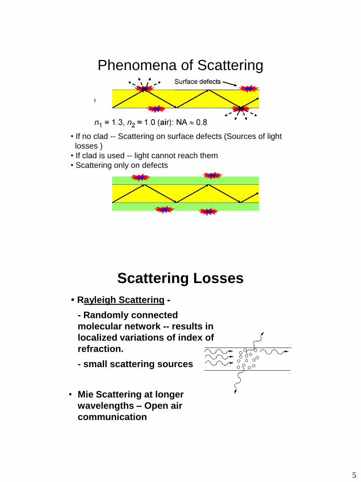
Phenomena of Scattering

• If no clad -- Scattering on surface defects (Sources of light

losses )

• If clad is used -- light cannot reach them

• Scattering only on defects

Scattering Losses

• Rayleigh Scattering -

- Randomly connected

molecular network -- results in

localized variations of index of

refraction.

- small scattering sources

• Mie Scattering at longer

wavelengths – Open air

communication

6

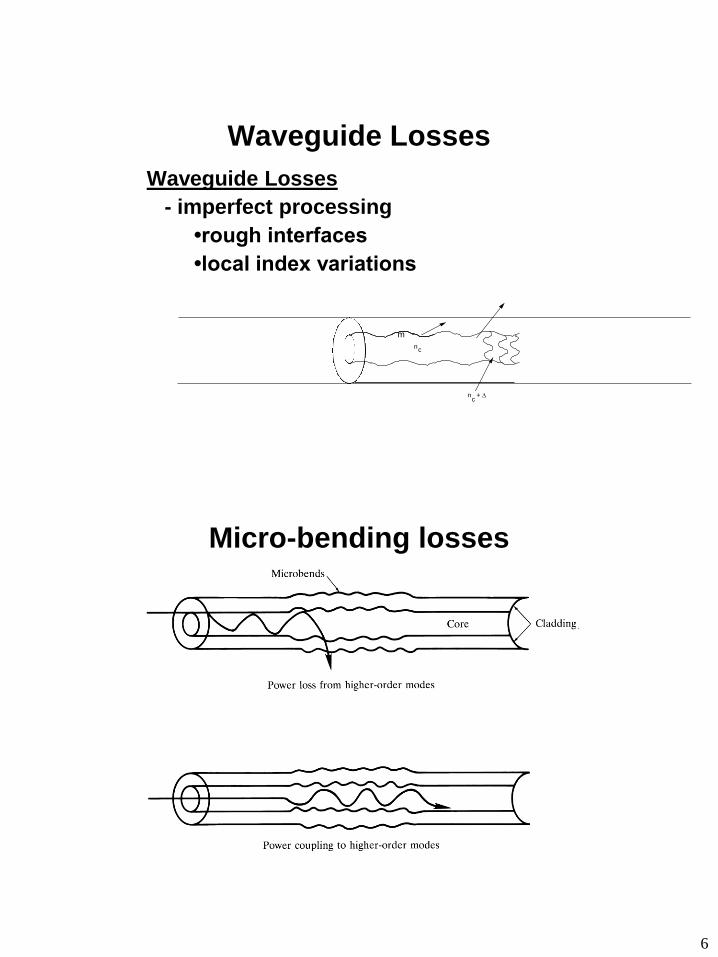
Waveguide Losses

- imperfect processing

•rough interfaces

•local index variations

m

nc

n + c

Waveguide Losses

Micro-bending losses

7

Power loss in a curved fiber

Power loss in curved fiber

Attenuation Measurements

• Cut off a length L

• Re-measure Pout

L

FiberP

in outP

8

Example

• Suppose 100 µW of power coupled in to a

fiber. In calculating attenuation losses of

this fiber it was observed that 8% of input

power to the fiber was absorbed/lost within

the fiber material. Calculate the output

power at the output of the fiber and losses

in dB. Take ncore = 1.45 and ncl = 1.42.

• Pin = 100 x 0.92 = 92 µW

• α = 0.362 dB

• Calculate the length of the fiber if losses

are 1 dB/km.

L = 362 m

9

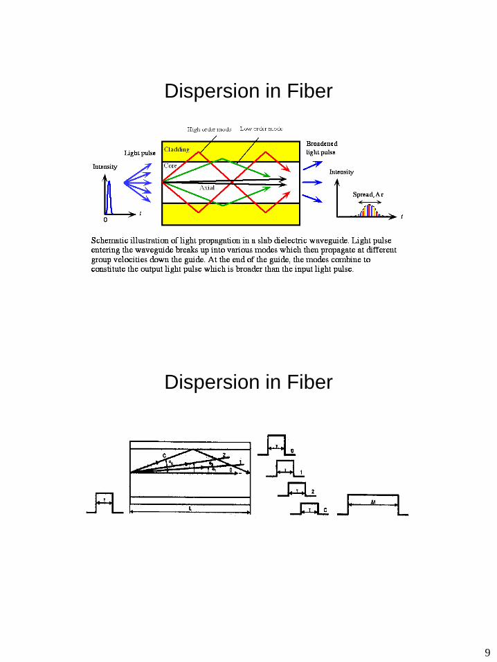
Dispersion in Fiber

Dispersion in Fiber

10

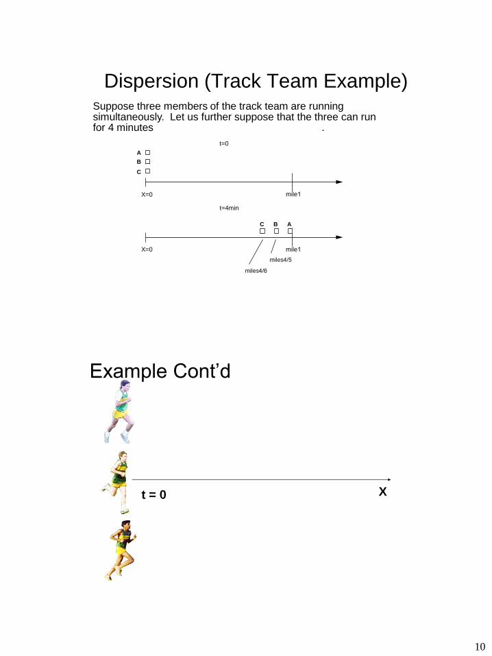
Dispersion (Track Team Example)Suppose three members of the track team are running simultaneously. Let us further suppose that the three can run

mile i ,for 4 minutes for persons A, B, and C respectively.

B

1mileX=0

1mileX=0

t=0

t=4min

A

C

ABC

4/5miles

4/6miles

Example Cont’d

t = 0 X

11

Example Cont’d

t = 4 min

X

Dispersion in Fiber

12

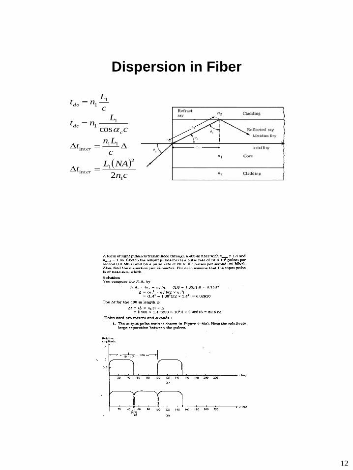
Dispersion in Fiber

c

Lntdo

11

c

Lnt

c

dccos

11

c

Lnt er

11int

cn

NALt er

1

2

1int

2

13

Intramodal or Chromatic

Dispersion

• In a single-mode fiber, the Intermodal (multi-path) dispersion is eliminated

• However, there is Chromatic dispersion

• It contains Material dispersion + Waveguide dispersion

• In a fiber, typically the material and waveguide dispersions counteract

• At about 1.3 -1.5 µm, the resulting dispersion may be close to zero.

• This is why the wavelength range of 1.3 -1.5 µm is the most promising for optical fiber communications

• Chromatic dispersion can be calculated as:

Chromatic Dispersion

LDtch

– D(λ) is the dispersion

coefficient or parameter

[ps/(nm.km)]

– Δλ is the linewidth

– L is the length

14

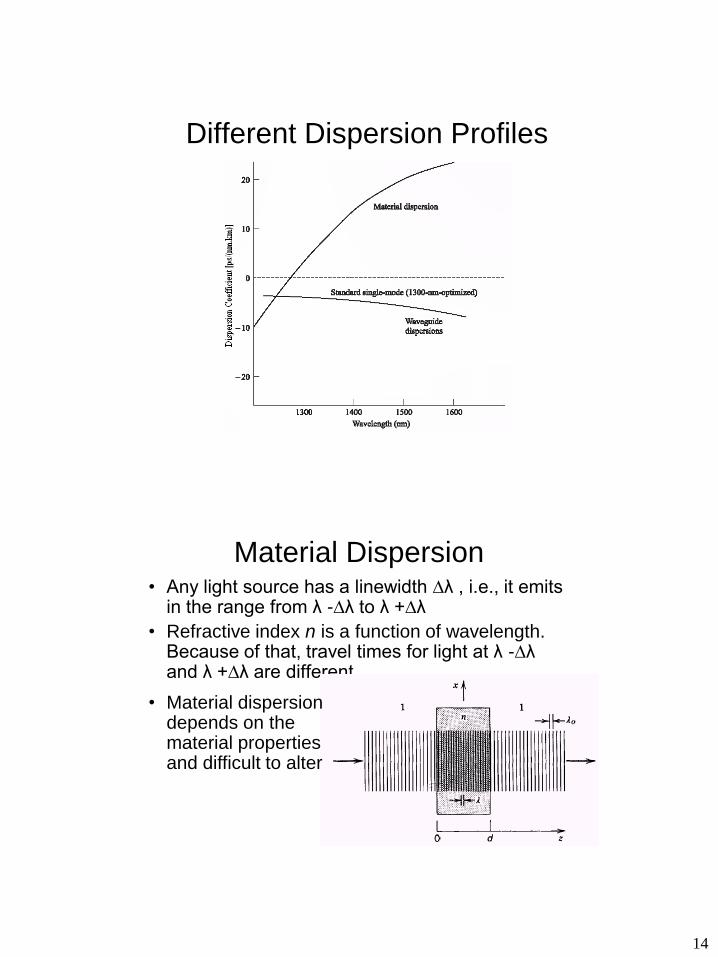
Different Dispersion Profiles

Material Dispersion • Any light source has a linewidth ∆λ , i.e., it emits

in the range from λ -∆λ to λ +∆λ

• Refractive index n is a function of wavelength. Because of that, travel times for light at λ -∆λ and λ +∆λ are different

• Material dispersion depends on the material properties and difficult to alter

15

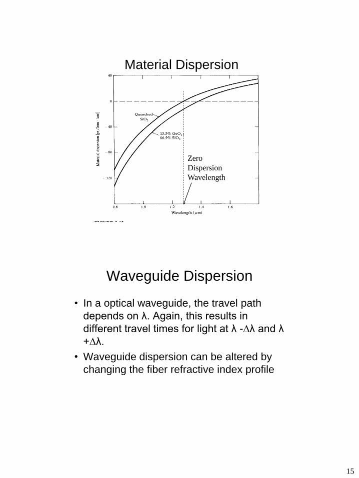
Material Dispersion

Zero

Dispersion

Wavelength

Waveguide Dispersion

• In a optical waveguide, the travel path

depends on λ. Again, this results in

different travel times for light at λ -∆λ and λ

+∆λ.

• Waveguide dispersion can be altered by

changing the fiber refractive index profile

16

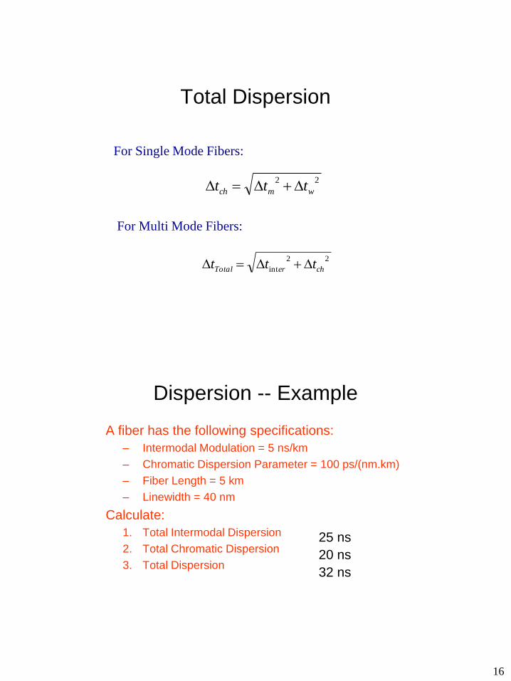
Total Dispersion

22

wmch ttt

For Single Mode Fibers:

For Multi Mode Fibers:

22

int cherTotal ttt

A fiber has the following specifications:

– Intermodal Modulation = 5 ns/km

– Chromatic Dispersion Parameter = 100 ps/(nm.km)

– Fiber Length = 5 km

– Linewidth = 40 nm

Calculate:

1. Total Intermodal Dispersion

2. Total Chromatic Dispersion

3. Total Dispersion

Dispersion -- Example

25 ns

20 ns

32 ns

17

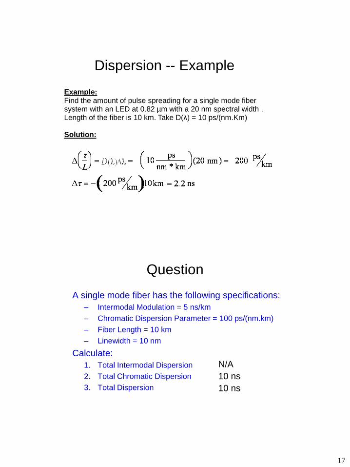
Dispersion -- Example

Example: Find the amount of pulse spreading for a single mode fiber system with an LED at 0.82 µm with a 20 nm spectral width . Length of the fiber is 10 km. Take D(λ) = 10 ps/(nm.Km)

Solution:

A single mode fiber has the following specifications:

– Intermodal Modulation = 5 ns/km

– Chromatic Dispersion Parameter = 100 ps/(nm.km)

– Fiber Length = 10 km

– Linewidth = 10 nm

Calculate:

1. Total Intermodal Dispersion

2. Total Chromatic Dispersion

3. Total Dispersion

Question

N/A

10 ns

10 ns

18

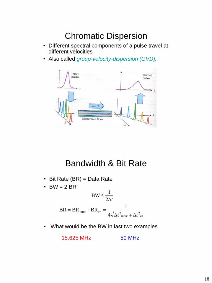
Chromatic Dispersion• Different spectral components of a pulse travel at

different velocities

• Also called group-velocity-dispersion (GVD),

Bandwidth & Bit Rate

• Bit Rate (BR) = Data Rate

• BW = 2 BR

• What would be the BW in last two examples

t

2

1BW

cher tt 2int

2chinter

4

1BRBRBR

15.625 MHz 50 MHz

19

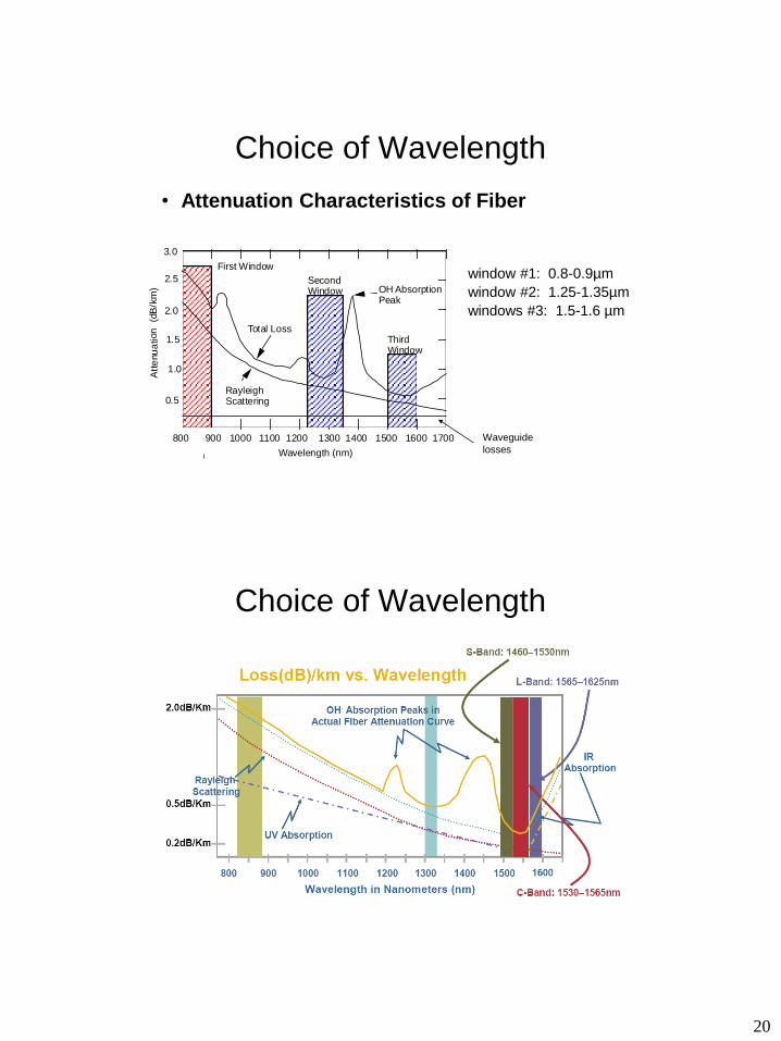
Choice of Wavelength

• Zero Dispersion Wavelength


20

window #1: 0.8-0.9µm

window #2: 1.25-1.35µm

windows #3: 1.5-1.6 µm

Rayleigh Scattering

Total Loss

Second Window

First Window

Third Window

800 900 1000 1100 1200 1300 1400 1500 1600 1700

3.0

2.5 2.0

1.5

1.0

0.5

OH Absorption Peak

Wavelength (nm)

Att

enu

ation

(d

B/k

m)

• Attenuation Characteristics of Fiber

Waveguide

losses



21

Transmission Bands

Bandwidth: over 35000 Ghz, but limited by bandwidth of EDFAs

(optical amplifiers): studied later…


Window Wavelength

(µm)

Source

Material

Applications

1 0.8-0.9 GaAs/

AlGaAs

Old

Communication

Systems

2 1.25-1.35 InP/

InGaAsP

LAN

3 1.5-1.6 Long-haul

Communication

Systems

Now LAN as well?

22

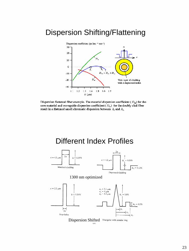
Modifying Chromatic Dispersion

• Material dispersion depends on the material properties and difficult to alter

• Waveguide dispersion can be altered by changing the fiber refractive index profile

– 1300 nm optimized

– Dispersion Shifting (to 1550 nm)

– Dispersion Flattening (from 1300 to 1550 nm)

Dispersion Shifting/Flattening

23

Dispersion Shifting/Flattening

Different Index Profiles

1300 nm optimized

Dispersion Shifted

24

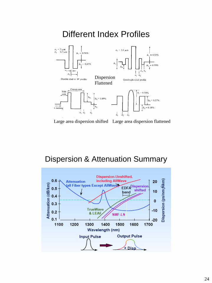
Different Index Profiles

Dispersion

Flattened

Large area dispersion shifted Large area dispersion flattened

Dispersion & Attenuation Summary

Fiber Pres 3

Documents

Transcript of Fiber Pres 3