Fiat Value in the Theory of Value

Edward C. Prescott Arizona State University,

Australian National University, and Federal Reserve Bank of Minneapolis

Ryan Wessel

Arizona State University

Staff Report 530

Revised June 2017

DOI: https://doi.org/10.21034/sr.530 Keywords: 100 percent reserve banking; Money in production function; Interest rate targeting; Inflation rate targeting; Friedman monetary satiation JEL classification: E0, E4, E5, E6 A preliminary version of this paper circulated under the title “Monetary Policy with 100 Percent Reserve Banking: An Exploration.” The views expressed herein are those of the authors and not necessarily those of the Federal Reserve Bank of Minneapolis or the Federal Reserve System. __________________________________________________________________________________________

Federal Reserve Bank of Minneapolis • 90 Hennepin Avenue • Minneapolis, MN 55480-0291

https://www.minneapolisfed.org/research/

1

Fiat Value in the Theory of Value

Edward C. Prescott1 Ryan Wessel2

March 17, 2016

Abstract

We explore monetary policy in a world without currency. In our world, money is a form of government debt that bears interest, which can be negative as well as positive. Services of money are a factor of production. We show that the national accounts must be revised in this world. Using our baseline economy, we determine the balanced growth paths for a set of money interest rate target policy regimes. Besides this interest rate, the only policy variable that differs across regimes is either the labor income tax rate or the inflation rate. We find that Friedman monetary satiation without deflation is possible. We also examine a set of inflation rate targeting regimes. Here, the only other policy variable that differs across policy regimes is the tax rate. There is a sequence of markets with outcome in each market being a Debreu valuation equilibrium, which determines the vector of assets and liabilities households take into the subsequent period. Evaluating a policy regime is an advanced exercise in public finance. Monetary satiation is not optimal even though money is costless to produce.

1 Arizona State University; Australian National University; Federal Reserve Bank of Minneapolis. E-mail: edward.prescott@asu.edu 2 Arizona State University. E-mail: ryan.wessel@asu.edu

2

Section 1: Introduction

Information processing technology is rapidly advancing and is changing the nature of the payment system. Currency is being used less and less to carry out transactions and to serve as a store of value. Indeed, a currency-less monetary system has become feasible and may be implemented at some point. All monetary systems need a unit of value, and the transition to a currency-less system would necessitate the creation of fiat value. A question is whether moving to a fiat value monetary system is socially desirable. This paper is a step toward addressing this important social question.

The equilibrium concept used in this study is Debreu’s [1954] valuation equilibrium. The commodity space in his framework is restricted only to being a linear topological space. In this study, there is a sequence of valuation equilibria with households entering a period with stocks of assets and liabilities. In the accounting period, economic outcomes are a valuation equilibrium. These outcomes, among other things, specify the stocks of assets and liabilities that households take into the subsequent accounting period. This is the way that the data are reported. These data are used to construct the national income and product accounts and balance sheets of the household and government sectors.

Large amounts of cash reserves are held by businesses. The amount relative to GDP is of the order of 1.3 annual GDP. Businesses hold these low-return assets for a reason—namely, for the services they provide. This leads us to treat the services of the money as a factor of production, or input to the aggregate production functions.3 Our production function is consistent with the money demand function when nominal interest rates are positive. It is also consistent with extended or even permanent periods of zero nominal interest rates. With the fiat value monetary system considered here, there is no currency, and for some policy regimes, the nominal interest rate paid on the money stock is negative and the real natural interest rate is positive.

A parametric set of neoclassical growth economies is considered. The benchmark economy is selected to match selected facts displayed by the pre-2008 U.S. economy given the values of the policy parameters in that period. For a set of policy regimes, the steady state of the benchmark economy is determined and comparisons made with the steady state of a number of policy regimes. These regimes include interest rate targeting policy regimes and inflation rate targeting regimes. For the interest rate regimes, both the inflation rate and the tax rate cannot be constant across regimes. We consider both a set of regimes for which the inflation rate is the same and the tax rate is different and a set of regimes for which the tax rate is the same and the inflation rate is different.

3 Many have suggested introducing money into the production function, including Fischer [1974], Friedman [1969], Sinai and Stokes [1972], and Orphanides and Solow [1990].

3

One finding is that in our currency-less monetary system, there can be Friedman satiation with positive inflation targeting regimes. This is possible because there is no currency that can be used as a store of value. Another finding is that monetary and fiscal policy cannot be completely separated. With the inflation targeting regimes, the tax rate on labor income is endogenous. This is because with interest rate targeting, the inflation rate has tax consequences for the government budget identity. We find that evaluating monetary policy is an advanced exercise in public finance.

In our model economies, there is a complete separation of the payment/transaction monetary system from the asset-management function system of the financial sector. Effectively, it is a 100 percent reserve system. Limited liability financial businesses that borrow from one group at a low rate and lend to another at a higher rate are not allowed. Financial businesses that pool assets of households and the businesses they own and manage these assets are permitted. With these businesses, investors share the returns. In the United States, most business financing is currently done this way. In our model world, there are no gains from having institutions that accept demand deposits and originate loans in order to make maturity transformation. Thus, there are no social gains from having fractional reserves banking. Further, there is no “too big to fail” problem for financial institutions.

The paper is organized as follows. Section 2 specifies the parametric set of neoclassical growth model economies used in this study. In Section 3, the benchmark economy in this set is specified by the policy parameters as well as the demographic, preference, and technology parameters. The model economy in our set matches the pre-2008 U.S. economy along selected dimensions. Section 4 transforms the variables in the standard way so that there is steady state in the transformed variables. The only policies that are considered are those for which there is a steady state. For any such policy, there is a unique steady-state equilibrium. Section 5 compares the balanced growth path for three sets of policy regimes. A policy is characterized by the values of seven variables. For a policy regime set, one of the seven variables is the target variable, and one variable is endogenous across regimes. For three sets of policy regimes, the steady states are determined. One has a money interest rate target with the tax rate endogenous. Another has a money interest rate target with the inflation rate endogenous. The third set has an inflation rate target with the tax rate endogenous. Section 6 discusses advantages and possible problems with the currency-less monetary system. Section 7 offers concluding comments.

Section 2: The Parametric Set of Model Economies

The analysis is steady state, and there is no uncertainty in living standards. Consequently, it does not matter whether an overlapping generations or infinitely lived family abstraction is used. We use the infinitely lived abstraction because it is easier to use.

Preference:

There is a measure 1 of identical households with preferences ordered by

(1) 0

[log log(1 )]tt t

tc hβ α

∞

=

+ −∑ ,

4

where 0tc > is consumption and [0,1]th ∈ is the fraction of the time endowment allocated to

the market. The parameter 1 / (1 ) (0,1)β ρ= + ∈ is the discount factor, and ρ is the discount

rate. The parameter α determines the relative shares of tc and the leisure fraction (1 )th− .

For the balanced growth path with balanced growth rate γ , the steady-state real interest rate is

(2) i γ ρ γ ρ= + + .

This fact will be exploited when characterizing the steady state for policies for which it exists.

Households hold two stocks of assets that they rent to the business sector. These stocks are non-human capital tk and (real) money tm . They also hold nominal government bonds tB .

Therefore, the households’ stock of real government bonds is /t t tb B P= . These three stocks

are the households’ state variable. Households also supply labor services th to the business

sector.

Price Level and Inflation:

There is a sequence of values for the composite output good in units of money. This is the definition of the price level tP at date t . We break with tradition and define the date t inflation

rate to be

(3) 1( ) /t t t tP P Pπ += − .

We do this because it simplifies and unifies notation. When constructing the real value of a variable—whether it is a stock, flows, or prices—we simply divide its nominal value by tP .

Aggregate Production Function

Technology advances at rate γ and is labor augmenting. Inputs to the business sector are the

services of non-human capital tk , the services of human capital th , and the services on real

money stock tm . Aggregate output is y . Variable z is the Cobb-Douglas aggregate of the

tangible and human capital services inputs:

(4) 1((1 ) )tt tz k hθ θγ −= + .

For these two stocks, one unit of stock provides one unit of services. We therefore use h and k to denote both the stocks and the service flows.

5

With constant returns to scale, one isoquant suffices to define the aggregate production function. The isoquant for y A= is plotted in Figure 1. In the three regions, the marginal products of money are

2

12 1

2 1

1

Region A (1 ) if

/Region B (1 ) if

Region C 0 if

y y m zm m

m zy y z m zm my m zm

f λ

λf λ λλ λ

λ

∂= − <

∂ −∂

= − ≤ ≤ ∂ − ∂

= >∂

In Region A, the elasticity of substitution between money m and composite input z is one. In this range, the normal demand for money relation holds. In Region C, the marginal product of money is zero; that is, there is money satiation. In Region B, the marginal product of money declines to zero as /m z declines from 2λ to 1λ .

6

Figure 1: Production Function Isoquant

If 2m zλ= , the bracketed term in the second line is one and the marginal product of money is

equal to that in the constant elasticity region. Similarly, if 1m zλ= , the bracketed term in the

second line is zero and the marginal product of money is equal to that in the zero elasticity region. The constant returns to scale production function with these isoquants is continuously differentiable.

The aggregate production function given the parameters 1 2{ , , , , }Aλ λ f θ is

12

11 2 2 1

11 1 2 1

m if

m ( , , , , ) if

z G( , , ) if

y Az m zy Az T m z z m zy A m z

f f

f f

f

λ

λ λ f λ λ

λ λ λ f λ

−

−

−

= <

= ≤ ≤

= > ,

where the functions T and G are

22

2 1 2 1

(1 ) (1 ) ( )2

1 2( , , , , ) ( )mzzT m z e

m

λ f f λλ λ λ λλλ λ f

− −−

− −=

7

2

2 1

(1 )12

1 21

( , , ) ( )G eλ fλ λ fλλ λ f

λ

−− −= .

The aggregate production function is increasing and concave, displays constant returns to scale, and is continuously differentiable.

Budget Constraints

Household

The assets held by the household are money, government debt, and capital. The inflation rate, possibly negative, is π ; government lump-sum transfers in cash or in kind are ψ ; kr and mr are

the rental price of capital k and real cash balances m ; bi and mi are the interest rates paid on

the two forms of government debt. A primed variable is the next-period value of that variable. With these notational conventions, the household real budget constraint is

'(1 ) '(1 )(1 ) ,k m b m

c x m bwh r k r m i b i m b m

π πτ ψ

+ + + + += − + + + + + + +

where x is capital investment given by

' (1 )x k kδ= − − .

This states that expenditures are for consumption, investment, currency acquisition, and government debt acquisition and that the receipts are equal to the after-tax labor income, rental income on (non-human) capital k , rental income on money, interest payments on the two forms of government debt, and lump-sum transfers received from the government.

We use capital letters to denote nominal quantities. In nominal terms, the date t household’s budget constraint is

1 1 (1 )t t t t t t t k t m t m t b t t t tC X M B W h r K r M i M i B M Bτ+ ++ + + = − + + + + + + +Ψ .

Here, tX is investment, so 1t t t tK K X Kδ+ = + − .

Firm

Given constant returns to scale, revenue is equal to costs, so

k my w h r k r m= + + .

8

Government

The government’s pure public good consumption is g . The interest rates on the two types of

government debt are mi and bi . The government’s budget constraint (expenditures equal

revenue plus deficit) is

[ '(1 ) ] [ '(1 ) ]m bg i m i b wh m m b bψ τ π π+ + + = + + − + + − .

Equivalently, the government budget constraint, using capital letters to denote nominal quantities, is

1 1( ) ( )t t mt t bt t t t t t t tG i M i B W h M M B Bτ + ++ Ψ + + = + − + − .

Equilibrium

Prices are 0{ , , , , }t kt mt bt mt tw r r i i ∞= . Equilibrium conditions are

(1) Households choose an optimal sequence of 1 1 1 0{ , , , , }t t t t t tc h k m b ∞+ + + = given prices and their

budget constraints.

(2) Firms choose at each date t the value maximizing { , , }t t th k m , given period t factor rental

prices.

(3) The government selection of 1 1 0{ , , , , , , }t t t t t mt t tg m b iψ τ π ∞+ + = is such that its budget constraints

for all t , given prices and the households’ decision variables, are satisfied.

Comment 1: The firm faces a sequence of static problems.

Comment 2: The list of elements specifying government policy includes both the prices and the quantities of money it issues. It will not be possible to target both the price and the quantity of money.

9

Section 3: Balanced Growth

The state of the household is its holdings at the beginning of the period real money stock, real government debt stock, and real capital stock. One important point is that interest rates are nominal. Nominal values of stocks and flows grow at the rate of inflation. Prices, with the exception of the interest rates on government bonds and money, grow at the inflation rate.

In a balanced growth equilibrium, output, consumption, investment, capital stock, money stock, debt stock, government expenditure, and transfers all grow at rate γ .

There are 19 variables to be determined. They are

{ , , , , , , , , , ', ', ', , , , , , , }k m b m g bw r r i i h k m b k m b g ψψ τ π f f f .

The following set of equilibrium conditions are necessary and sufficient for a steady state for a given policy and are used to find the steady state.

From the firm’s maximization problem: three marginal conditions are that the marginal products (MPs) of the factors of production are equal to their rental prices. There is the zero profit condition given constant returns to scale. Aggregate feasibility is another condition.

(E1) k kMP r=

(E2) hMP w=

(E3) m mMP r=

(E4) k mc x g r k r m wh+ + = + +

(E5) y c x g= + +

Variable y is the output of the business sector and does not include the government production of money.

From the households’ maximization problem: the intratemporal marginal condition is that the marginal rate of substitution between consumption and leisure is equal to the ratio of their after-tax prices. The intertemporal condition is that the marginal rate of substitution between consumption in this period and consumption in the next period equals the ratio of their prices. These conditions are

(E6) \ (1 ) (1 )c h wα τ− = −

10

(E7) 1 (1 )(1 )kr γ ρ δ+ = + + +

(E8) 1 (1 )(1 )(1 )bi ρ π γ+ = + + +

(E9) b m mi i r= +

(E10) [ ' (1 ) ] '(1 ) '(1 ) (1 ) (1 ) (1 )k b m mc k k m b wh r k i b i r mδ π π τ ψ+ − − + + + + = − + + + + + + + .

E8 and E9 are no-arbitrage conditions. Because there is no uncertainty, the household return on money and government bonds must be equal, and the return on government bonds must be equal to the return on investing in k.

Balanced growth requires

(E11) ' (1 )b bγ= +

(E12) ' (1 )m mγ= +

(E13) ' (1 )k kγ= + .

The law of motion of capital is

(E14) ' (1 )k k xδ= − + .

In each of the sequence of valuation equilibria, there are three government policy constraints and a government budget constraint (expenditures equal revenue plus deficit):

(E15) gg yf=

(E16) yψψ f=

(E17) bb yf=

(E18) [ '(1 ) ] [ '(1 ) ]m bg i m i b wh m m b bψ τ π π+ + + = + + − + + − .

The set of policy variables is { ,m/ y, , }mi τ π . Values for two of these four variables are chosen. A

restriction is that variables mi and /m y are not both chosen. This adds two equations to our

set of necessary equations. Thus, there are 20 equations in 19 unknowns. By Walras’ law, one of the budget constraints is redundant.

Section 4: Baseline Economy for Balanced Growth Analyses

11

A parametric set of economies has been specified. For the baseline economy, a parameter vector is chosen so that the baseline economy has a balanced growth that roughly matches the U.S. economy in consumption and investment shares, fraction of time worked, asset stocks to output ratios, factor income shares, inflation rate, and after-tax return on capital. Table 1 displays the national accounts for our chosen baseline economy.

12

Table 1 – National accounts for the baseline economy

Product and Income Accounts Product 1.08

Household Consumption 0.68 Government Consumption 0.05 Capital Investment 0.27 Money Investment 0.08

Income 1.08 Wages 0.64 Depreciation of Capital 0.15 Capital Rental Income 0.19 Money Rental Income 0.01 Central Bank Profits 0.08

Government Accounts

Receipts 0.43 Tax Revenue 0.33 Money Issuance 0.08 Debt Issuance 0.03

Expenditures 0.43

Government Consumption 0.05 Transfers to Household 0.25 Bond Services 0.04 Money Services 0.10

Asset Stocks

Capital 3.81 Money 1.50 Bonds 0.50

Other

Hours Worked 0.40 Labor Income Share 0.64

The annual growth rate is 3 percent.

13

The size of the stock of money may seem large. The 1.5 times annual GNP stock is much larger than M2, which is about 0.6. As pointed out by Williamson [2012], two types of money are used for transaction purposes. Much of the liquid government debt is held as cash reserves, and in 2015 the nominal return on this debt in the major advanced industrial countries was near zero. Businesses make large payments using the shadow banking sector and small payments using the commercial banking system. The proposed arrangement has only one type of money.

Because money services are a factor of production, the national accounts must be revised so that they are consistent with the theoretical framework being used. Money, like capital, provides services to the business sector; therefore, there must be a “Money Rental Income” entry on the income side of the accounts and a “Money Investment” entry on the product side of the accounts. The government costlessly produces money and earns monopoly profits. These profits are entered on the income side of the national accounts as the entry “Central Bank Profits.”

Table 2 displays the set of government policy parameters for the baseline economy. Note that the total factor productivity (TFP) parameter A is chosen for convenience so that y is one, and thus levels and levels relative to y are the same in the baseline economy. Also, the value of the satiation parameter 2λ is somewhat arbitrary. It was set high enough so that the baseline

economy is not satiated with money.

Table 2 – Policy parameter values for the baseline economy

Policy Parameters /g y government public goods share / yψ transfer share /m y money-output ratio

/b y privately held gov. debt to output τ labor tax rate

mi interest rate on money

bi interest rate on gov. bonds π inflation rate (annual %)

.05 0.25

1.5 0.5

0.52 6.54% 7.21% 2.00%

Table 3 lists the calibrated values of the preference and technology parameters.

14

Table 3 – Preference and technology values for baseline economy

Preference and Technology Parameters Values α relative preference for leisure β discount rate (annual) δ depreciation rate (annual) γ technical growth rate θ capital cost share φ money cost share A TFP λ money satiation parameter

0.68 0.98 0.04 0.03 0.35 0.01 1.13 2.00

15

Section 5: Three Explorations

In this section, we will explore the consequences of various monetary policy regimes under our alternative financial system. Our assessment is that technology has changed sufficiently so that existing monetary theory does not predict the consequences of monetary policy regimes. Currently, there is public discussion as to whether the interest rate should be increased and what the inflation rate target should be. Exploration 1 will explore the consequences of various money supply—or, equivalently, money interest rate—policy regimes. Exploration 2 will explore the consequences of various inflation rate targeting regimes.

For this analysis, we focus only on monetary policy and therefore minimize the role of fiscal policy. This is done by keeping fiscal policy parameters as fixed as possible.4 Thus, the lump-sum transfers and the size of public goods consumption relative to output are held fixed. We also keep the value of non-monetary government debt at a fixed fraction of output. The inflation rate has tax consequences; this requires that the labor tax rate be endogenous when comparing the balanced growth paths of policies with different inflation rates. The three remaining policy variables enter the government budget constraint and therefore have some fiscal consequences.

For our explorations, the set of government policy variables includes the inflation rate, the tax rate, and the interest paid on money. In each exploration, two of these policy variables are fixed, and two are endogenous.

Our measure of welfare across policy regimes is consumption equivalent (CE) welfare. We report the percentage change in consumption that must be given to an individual to make him indifferent among worlds with different policy regimes. We acknowledge that this measure of welfare is a steady-state comparison for one type and does not take into account transitional concerns. But given that the ratio of non-human capital to output is the same for all balanced growth paths, the consequences of transition for the policy regimes comparisons we consider are small.

4 Sargent and Wallace [1981], in their dynamic general equilibrium analysis, find that monetary and fiscal policy cannot be completely separated.

16

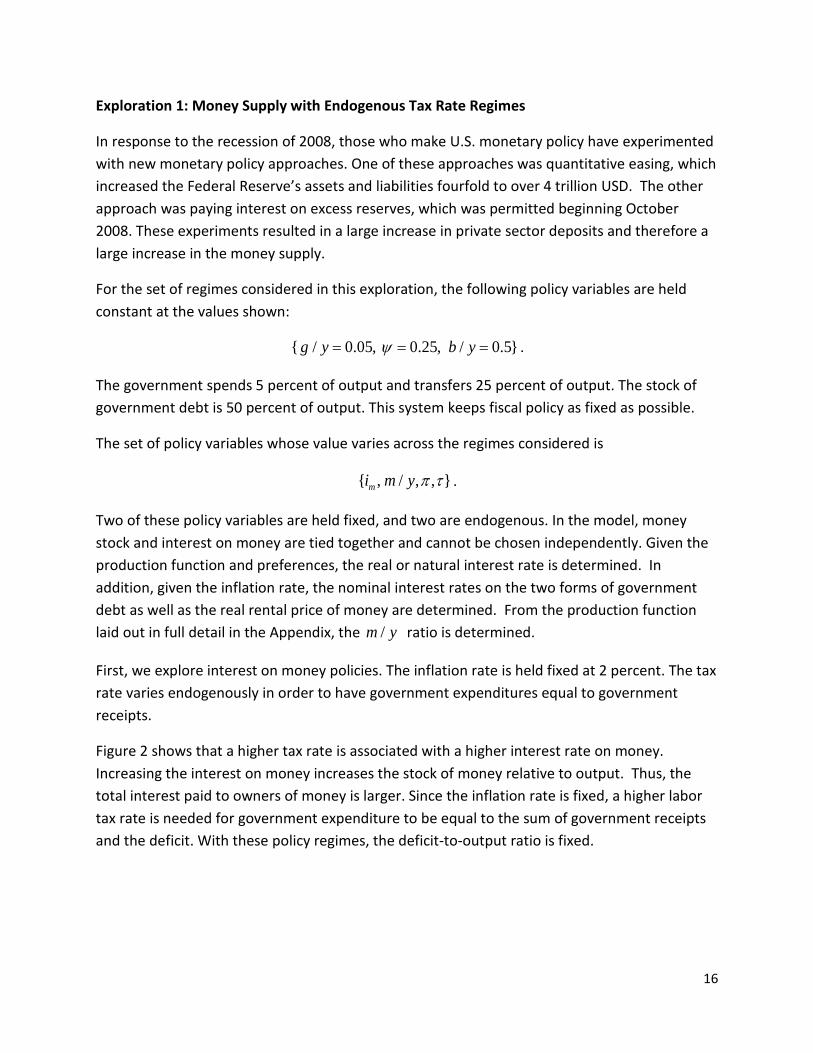
Exploration 1: Money Supply with Endogenous Tax Rate Regimes

In response to the recession of 2008, those who make U.S. monetary policy have experimented with new monetary policy approaches. One of these approaches was quantitative easing, which increased the Federal Reserve’s assets and liabilities fourfold to over 4 trillion USD. The other approach was paying interest on excess reserves, which was permitted beginning October 2008. These experiments resulted in a large increase in private sector deposits and therefore a large increase in the money supply.

For the set of regimes considered in this exploration, the following policy variables are held constant at the values shown:

{ / 0.05, 0.25, / 0.5}g y b yψ= = = .

The government spends 5 percent of output and transfers 25 percent of output. The stock of government debt is 50 percent of output. This system keeps fiscal policy as fixed as possible.

The set of policy variables whose value varies across the regimes considered is

{ , / , , }mi m y π τ .

Two of these policy variables are held fixed, and two are endogenous. In the model, money stock and interest on money are tied together and cannot be chosen independently. Given the production function and preferences, the real or natural interest rate is determined. In addition, given the inflation rate, the nominal interest rates on the two forms of government debt as well as the real rental price of money are determined. From the production function laid out in full detail in the Appendix, the /m y ratio is determined.

First, we explore interest on money policies. The inflation rate is held fixed at 2 percent. The tax rate varies endogenously in order to have government expenditures equal to government receipts.

Figure 2 shows that a higher tax rate is associated with a higher interest rate on money. Increasing the interest on money increases the stock of money relative to output. Thus, the total interest paid to owners of money is larger. Since the inflation rate is fixed, a higher labor tax rate is needed for government expenditure to be equal to the sum of government receipts and the deficit. With these policy regimes, the deficit-to-output ratio is fixed.

17

Figure 2: Labor tax rates for different interest rate targets

Figure 3 shows that there is a steady-state welfare-maximizing interest rate on money. A regime with a higher interest rate on money has a larger money services input to aggregate production. However, a higher interest rate regime also has a smaller labor input to aggregate production. For low interest rate regimes, the output increases because the larger money service input exceeds the output reduction arising from lower labor supply. For high interest rate regimes, output decreases because the reduction in output from lower labor supply exceeds the increase in output from larger money services. Figure 3 shows that, for our model economy, welfare is highest in a world where the interest rate on money is approximately 6 percent.

Figure 3: Steady-state welfare indicator for various interest rate targets

18

The nominal interest rate on government bonds is 7.2 percent. Why would the welfare-maximizing interest rate policy regime not completely eliminate the gap between the interest on money and bonds; that is, why is monetary satiation not optimal? Because we have fixed inflation and government spending, a labor tax rate change is needed for balance in the government accounts.

This highlights the importance of fiscal response to monetary policy. In a regime that targets the inflation rate, fiscal policy must respond to changes in interest rate policy.

Exploration 2: Money Stock Policy with Inflation Rate Regimes

Next, we explore money stock policy regimes. We fix the labor tax rate at 52 percent and allow the inflation rate to vary endogenously to ensure that government expenditures are equal to government receipts. We consider money stock policies associated with both satiation and non-satiation.

Figure 4 shows that larger money stock regimes have higher steady-state welfare. However, increasing the money stock increases welfare only up to the satiation point, beyond which increasing the money stock does not increase welfare. For policy regimes with satiation, money and government debt are equivalent. In these regimes, money plus government debt is a constant, and consequently there is an unimportant indeterminacy.

Figure 4: Steady-state welfare indicator for various money stock regimes

Satiated Economies

19

In figure 5, we see that for satiated money stock regimes, the rental price of money services is zero. For these regimes, the marginal product of money is equal to the marginal cost of producing money (assumed to be zero). Interest rates on money and bonds are equal, and money and bonds are identical government debt instruments.

In the United States, policies that increase the money stock are enacted by the central bank purchasing government bonds from banks in exchange for money. Since money and bonds are identical in satiated economies, the split of total government debt between money and bonds is indeterminate. In the satiated region, the sum of money and bonds is constant.

The Friedman rule leads to satiation in economies in which money is not a factor of production. The Friedman rule is to deflate at the real interest rate [Friedman, 1960]. The return on currency is then equal to the return on capital. In the monetary system considered here, we eliminate the inefficiency not by deflating at the real interest rate but by choosing a money stock regime that leads to a satiated economy. We call this state “Friedman satiation.”

When money is a factor of production, Friedman satiation can occur with a range of inflation targets, including positive inflation. This feature allows for Friedman satiation without the difficulties associated with negative inflation rates [see McAndrews, 2015]. For example, Friedman satiation occurs when the target inflation rate is 2 percent, the tax rate is 53.5 percent, and the ratio of money stock to output is 1.75.

Figure 5: Marginal product of money for various money stock regimes

Satiated Economies

20

Exploration 3: Inflation Rate Targeting with Endogenous Tax Rate Regimes

The inflation rate has been of particular interest of late. The U.S. Federal Reserve Board has been vocal about wanting to increase the inflation rate to the “normal” rate of 2 percent. Many have been puzzled by the persistently low inflation rate, which is currently near zero and is expected to stay under 2 percent for the next 30 years.5 However, is low inflation a bad thing? Since price stability is part of a Federal Reserve congressional mandate, a theory that can address inflation rate targeting regimes is needed.

In this section, the interest rate on money is held fixed so that we can focus on the consequences of inflation rate targeting regimes. Various inflation rate policies are chosen. We consider only policies for which there is not satiation. This restricts the inflation rate target to be greater than or equal to 1.9 percent. The tax rate varies endogenously in order to have government expenditures equal to government receipts. Since interest on money is held fixed, the money stock also varies endogenously across policies.

Figure 6 shows that a higher labor tax rate is associated with a lower inflation rate regime. Inflation is a form of tax on money. A higher inflation rate regime has a lower labor income tax rate, higher labor supply, and higher consumption. This raises the interesting possibility of using a money tax to reduce the labor distortion created by financing the government through labor income tax.

Figure 6: Labor tax rates for inflation rate targeting regimes

5 Subtract the expected return on inflation-indexed Treasury securities from the expected return on nominal Treasury securities to see this.

21

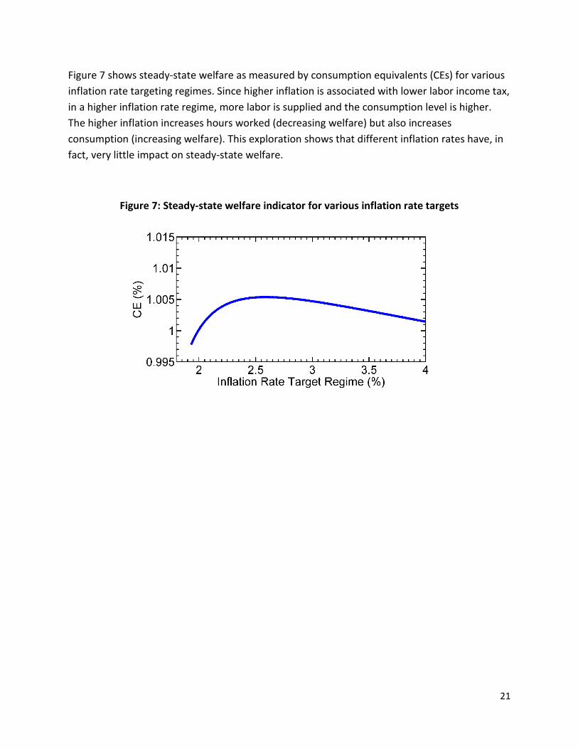
Figure 7 shows steady-state welfare as measured by consumption equivalents (CEs) for various inflation rate targeting regimes. Since higher inflation is associated with lower labor income tax, in a higher inflation rate regime, more labor is supplied and the consumption level is higher. The higher inflation increases hours worked (decreasing welfare) but also increases consumption (increasing welfare). This exploration shows that different inflation rates have, in fact, very little impact on steady-state welfare.

Figure 7: Steady-state welfare indicator for various inflation rate targets

22

Section 6: Possible Problems and Advantages

Some problems with this system are apparent. Privacy protection would need to be considered. We will not deal with this more general problem here. Also, in an environment in which banks are purely deposit institutions, shadow banking might develop and pose a problem.

This potential shadow banking problem has a possible solution. To effectively eliminate businesses that borrow low from one group and lend high to another, the government could tax net interest income at a 100 percent rate for limited liability businesses. This approach would remove any incentive to engage in shadow banking.

Our proposed reforms also have possible advantages. First, bank runs would be prevented because depositors would have no place to run to.6 Whenever a transaction takes place between private agents, one party's demand deposit account is credited by the amount of the transaction, and the other party’s demand deposit account is debited by the same amount.

Second, our reforms would eliminate the need for costly regulations, as is associated with the U.S. deposit insurance system. A 100 percent reserve requirement would eliminate the need for stress tests and regulatory entities to ensure that banks are not taking on excessive risk. These activities cost about one-half percent per year per dollar deposited at commercial banks. This amount represents a non-negligible cost.

One claimed cost of the monetary system we explore is that it would increase the cost of financing because of the higher commercial bank equity cost. This argument is that with 100 percent reserve banking, bank equity would be higher and bank equity is costly. Admati and Hellwig [2013] establish that bank equity is not costly. With our monetary system, demand deposits are what households and businesses choose to hold. Another claim often made is that fractional reserve banking is valuable in providing maturity transformation because agents want to lend short and borrow long. The agents in our world can hold as much money as they want; that is, they can lend short as much as they want. There is no need for maturity transformation.

We emphasize that much needs to be done before the theory can be used to predict the consequences of alternative policy. As done in McGrattan and Prescott [2016] for the consequences of an alternative tax policy regime, demographic projections must be made and introduced into the model economy being used. In addition, the equilibrium transition path to the balanced growth path for the alternative policy regime must be determined.

6 A number of economists have proposed a 100 percent reserve for demand deposits as an arrangement that is not prone to bank runs. They include Fisher [1936] and Friedman [1960], and more recently Cochrane [2014], Prescott [2014], and Smith [2013].

23

Section 7: Concluding Comments

We explore an alternative financial system that is possible given the current state of information processing technology. Before this system could be implemented, existing law would have to be changed to permit business enterprises to hold interest-bearing money.

This exploration is warranted because, in our assessment, existing theory does not provide predictions about the consequences of alternative monetary policy regimes. The trial-and-error approach that characterizes current monetary policy is fraught with danger. With better theory, alternative monetary systems can be assessed without experimentation. We hope that this paper fosters fruitful theoretical work on reforming the payment system in response to advances in information processing technology.

By integrating money into valuation theory, the tools of aggregate public finance can be and are applied. This is not the first use of these tools to quantitatively predict the consequences of alternative monetary policy regimes. Previous studies modeled the households’ holding of M1, which was held for transaction purposes. It was motivated by Meltzer’s [1963] finding of a reasonably stable M1 velocity depending on the short-term interest rate. Lucas and Stokey [1987] develop a transaction-based theory of this transaction demand for money. Cooley and Hansen [1989] introduced the Lucas-Stokey theory with cash and credit goods into the neoclassical growth model and carried out a quantitative general equilibrium analysis of the cost of modest inflation.

This transaction-based theory does not account for the large holding of cash reserves by businesses. Hodrick [2013] reports that in 2013, the cash reserves of American businesses were nearly equal to annual GNP. This does not include the cash reserves of businesses in the household sector. Households accumulate cash reserves so that they can buy a car or make a down payment on a residence. One implication is that much of M3 is made up of the cash reserves held by household businesses. Cash reserves are held by businesses because they are productive assets that facilitate the operation of the business sector.

24

References

Admati, Anat R., and Martin F. Hellwig. 2013. The Bankers’ New Clothes: What’s Wrong with Banking and What to Do about It. Princeton, NJ: Princeton University Press.

Cochrane, John H., 2014. "Monetary Policy with Interest on Reserves.” Journal of Economic Dynamics and Control, 49 (December), 74–108.

Cooley, Thomas F., and Gary D. Hansen. 1989. “The Inflation Tax in a Real Business Cycle Model.” American Economic Review, 79 (4), 733–748.

Debreu, Gerard. 1954. “Valuation Equilibrium and Pareto Optimum.” Proceedings of the National Academy of Sciences of the United States of America, 40 (7), 588–592.

Fischer, Stanley. 1974. “Money and the Production Function.” Economic Inquiry, 12 (4), 517–533.

Fisher, Irving. 1936. 100% Money and the Public Debt. Rev. ed. New York: Adelphia.

Friedman, Milton. 1960. A Program for Monetary Stability. New York: Fordham University Press.

Friedman, Milton. 1969. “The Optimum Quantity of Money.” In The Optimum Quantity of Money and Other Essays. Chicago: Aldine.

Hodrick, Laurie Simon. 2013. “Are U.S. Firms Really Holding Too Much Cash?” SIEPR Policy Brief, July.

Lucas, Robert E., Jr., and Nancy L. Stokey. 1987. “Money and Interest in a Cash-in-Advance Economy.” Econometrica, 55 (3), 491–513.

McAndrews, James. 2015. “Negative Nominal Central Bank Policy Rates: Where Is the Lower Bound?” Speech, Federal Reserve Bank of New York, May 8.

McGrattan, Ellen R., and Edward C. Prescott. 2016. “On Financing Retirement with an Aging Population.” Quantitative Economics, 8 (1), 75–115.

Meltzer, Allen H. 1963. “The Demand for Money: The Evidence from the Time Series.” Journal of Political Economy, 71 (3), 219–246.

Orphanides, Athanasios, and Robert Solow. 1990. “Money, Inflation, and Growth.” In Handbook of Monetary Economics, Vol. 1, edited by B. M. Friedman and F. H. Hahn, 223–261. Amsterdam: Elsevier.

25

Prescott, Edward C. 2014. “Interest on Reserves, Policy Rules and Quantitative Easing.” Journal of Economic Dynamics and Control, 49 (December), 109–111.

Sargent, Thomas J., and Neil Wallace. 1981. “Some Unpleasant Monetarist Arithmetic.” Federal Reserve Bank of Minneapolis Quarterly Review, 5 (3), 1–17.

Sinai, Allen, and Houston H. Stokes. 1972. “Real Money Balances: An Omitted Variable from the Production Function?” Review of Economics and Statistics, 54 (3), 290–296.

Smith, Andrew D. 2013. “How to Make a Run-Proof Bank: Achieving Maturity Transformation without Fractional Reserves.” Paper presented at Australian Conference on Economics, July 10.

Williamson, Stephen D. 2012. "Liquidity, Monetary Policy, and the Financial Crisis: A New Monetarist Approach." American Economic Review, 102 (6): 2570–2605.