FFT in quantum physics - Prace Training Portal: Events · A fast Fourier transform (FFT) is an...
40
FFT in quantum physics Maciej E. Marchwiany, Maciej Szpindler
Transcript of FFT in quantum physics - Prace Training Portal: Events · A fast Fourier transform (FFT) is an...

FFT in quantum physicsMaciej E. Marchwiany, Maciej Szpindler
2
Table of contents
●Fourier tansform●FFT●Poisson equation●Solving Poisson equation●Poisson equation in DFT●P3DFFT●P3DFFT: initialization●P3DFFT: Array Decomposition●P3DFFT: Forward transform●P3DFFT: Backward transform
3
Fourier transform
FT :ℝN→ℂ
N
The Fourier transform is a mathematical operation with many applications in physics and engineering that expresses a mathematical function of time as a function of frequency, known as its frequency spectrum; Fourier's theorem guarantees that this can always be done.
4
Applications
● engineering● signal processing● electronics● cosmology ● NMR spectroscopy● quantum chemistry● computational material science● ...

5
Fourier transform
f ∈L1 ℝN
f k =∫ℝ
N f x e−2 i x k d x
f k = 1
2π N ∫ℝ
N f x e−2 i xk d x
f k = 1
2π N /2∫ℝ
N f x e−2 i xk d x

6
Inverse Fourier transform
f x =1
2πN∫ℝ
N f k e2 i k xd k
f k =∫ℝ
N f x e2 i k xd k
f k = 1
2π N /2∫ℝ
N f x e2 i k x d k
f k =∫ℝ
N f x e−2 i x k d x
f k = 1
2π N ∫ℝ
N f x e−2 i xk d x
f k = 1
2π N /2∫ℝ
N f x e−2 i xk d x

7
Interpretation

8
Discrete Fourier transform
xk=∑ xne−2i π
kN
nxn=
1N
∑ xk e2i π
kN
n
∫dx →∑n
k=k0,k1,…, kN−1
9
FFT
A fast Fourier transform (FFT) is an efficient algorithm to compute the discrete Fourier transform (DFT) and its inverse. There are many distinct FFT algorithms involving a wide range of mathematics, from simple complex-number arithmetic to group theory and number theory.
By far the most common FFT is the Cooley–Tukey algorithm. This is a divide and conquer algorithm that recursively breaks down a DFT of any composite size N = N1N2 into many smaller DFTs of sizes N1 and N2, along with O(N) multiplications by complex roots of unity traditionally called twiddle factors (after Gentleman and Sande, 1966).
10
FFT algorithms
● Cooley–Tukey algorithm● Prime-factor FFT algorithm● Bruun's FFT algorithm● Rader's FFT algorithm● Bluestein's FFT algorithm● Odlyzko–Schönhage algorithm
11
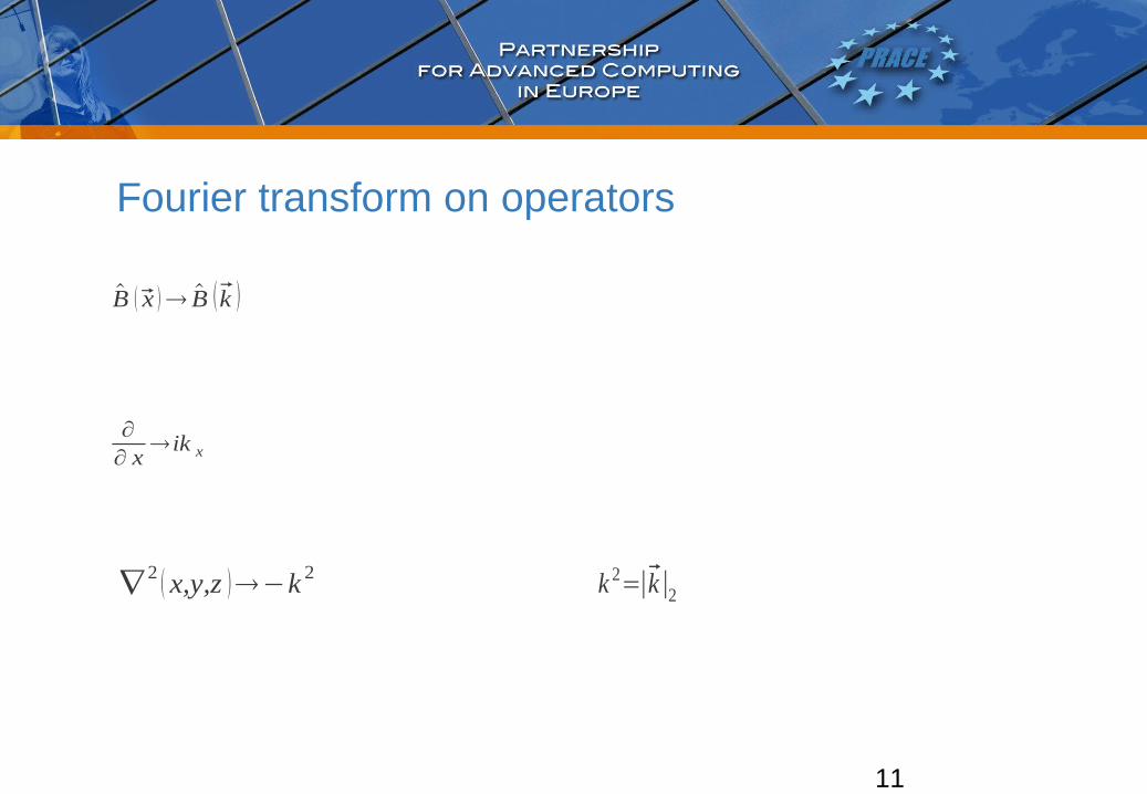
Fourier transform on operators
B x B k
∂
∂ x ik x
∇2 x,y,z −k 2 k 2=∣k∣2

12
Poisson equation
∇2V H r =−4 πρ r
V H r
ρ r
V H r =∫ρ R
∣r−R∣d R Coulomb potential
−k 2V Hk =−4πρ k
Electrons density
13
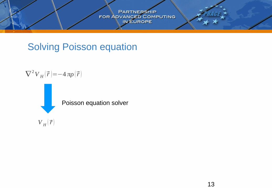
Solving Poisson equation
∇2V H r =−4 πρ r
V H r
Poisson equation solver
14
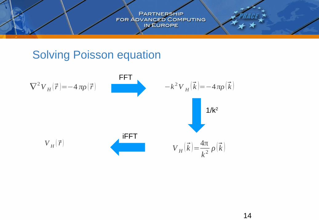
Solving Poisson equation
∇2V H r =−4 πρ r −k 2V H
k =−4πρ k
V H k =4π
k 2ρ k V H r
FFT
iFFT
1/k2

15
k=0
k=0
ρ k=0 =∫ ρ x d x=⟨ ρ⟩
mean value of x⟨ x ⟩
f k=0=∫ℝN f x e−2 i x 0d x=∫ℝN f x d x

16
k=0
⟨ ρ⟩=0 ρ k=0 =0
17
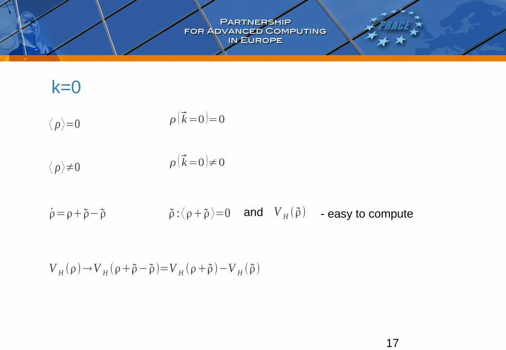
k=0
⟨ ρ⟩=0 ρ k=0 =0
⟨ ρ⟩≠0 ρ k=0 ≠0
and - easy to compute= − : ⟨ ⟩=0
V H V H − =V H −V H
V H
18
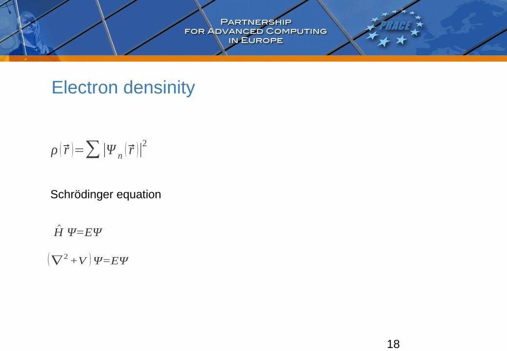
Electron densinity
ρ r =∑∣Ψ n r ∣2
Schrödinger equation
∇ 2+V Ψ=EΨ
H Ψ=EΨ

19
Wave function in 1D
Ψ r =Ae ikr+Be−ikr
Ψ r =a sin kr +b cos kr
Ψ r =a sin kr
∫ d r∣Ψ r ∣2=1
V r :Ψ 0 =0∧Ψ L =0
∇ 2+V r Ψ r =EΨ r
∂2
∂r 2+V r Ψ r =EΨ r
k=nπL
n∈ℤ
20
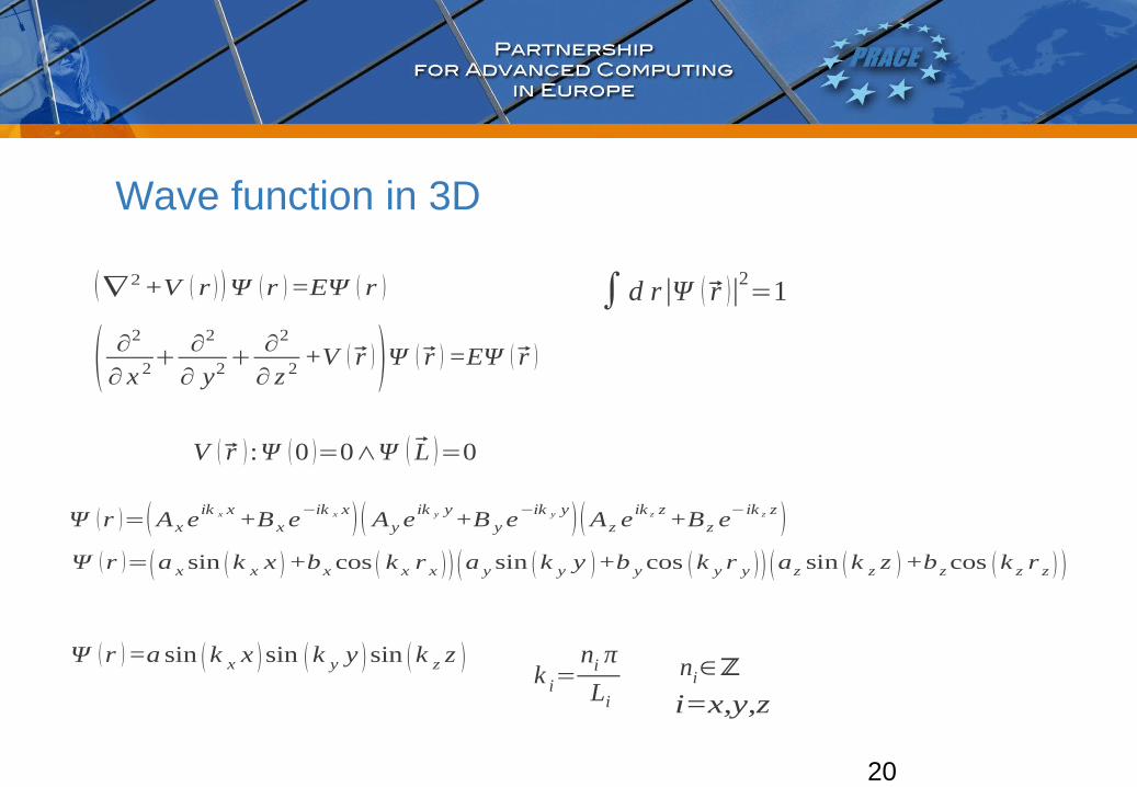
Wave function in 3D
Ψ r =Ax eik x x+B x e
−ik x x Ay eik y y+B y e
−ik y y A z eik z z+B z e
−ik z z Ψ r =a x sin k x x +bx cos k x r x a y sin k y y +b y cos k y r y az sin k z z +b zcos k z r z
Ψ r =a sin k x x sin k y y sin k z z
∫ d r∣Ψ r ∣2=1
V r :Ψ 0 =0∧Ψ L =0
∇ 2+V r Ψ r =EΨ r
∂2
∂ x 2
∂2
∂ y2
∂2
∂ z 2+V r Ψ r =EΨ r
k i=ni π
Li
ni∈ℤ
i=x,y,z

21
Electron densinity
ρ r =∑∣Ψ n r ∣2
ρ r =a2sin2 k x x sin2 k y y sin2 k z z
22
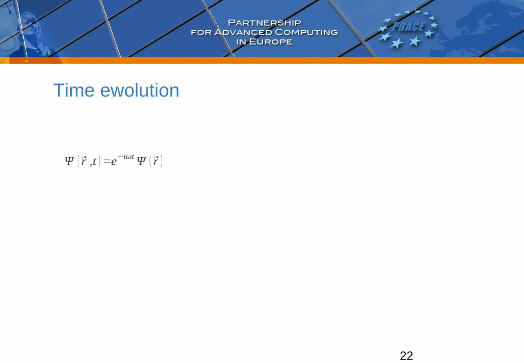
Time ewolution
Ψ r ,t =e−iωtΨ r
23
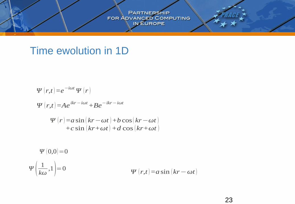
Time ewolution in 1D
Ψ 0,0 =0
Ψ r,t =a sin kr−ωt
Ψ r,t =e−iωtΨ r
Ψ r,t =Ae ikr−iωt+Be−ikr−iωt
+c sin kr+ωt +d cos kr+ωt Ψ r =a sin kr−ωt +b cos kr−ωt
Ψ 1kω
,1=0
24
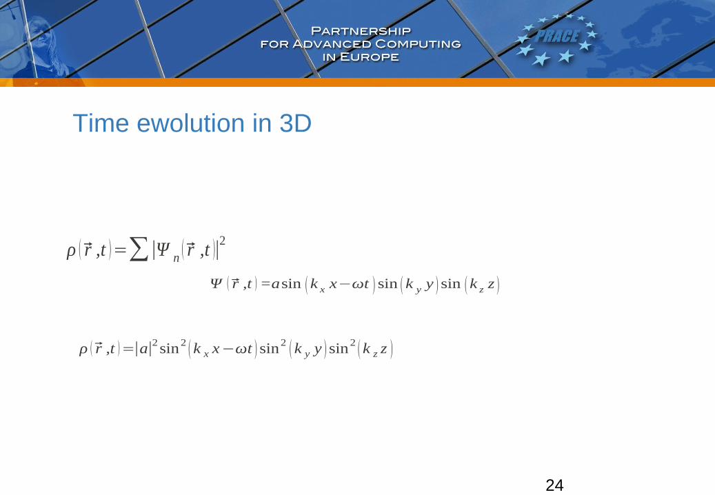
Time ewolution in 3D
ρ r ,t =∑∣Ψ n r ,t ∣2
Ψ r ,t =asin k x x−ωt sin k y y sin k z z
ρ r ,t =∣a∣2sin2 k x x−ωt sin2 k y y sin2 k z z
25
DFT library
FFTW P3DFFT GSL ACML ESSL FFTPACK FFTEASY JTransforms GPUFFTW ...
26
Deklaracja biblioteki
#include "p3dfft.h"
#include <mpi.h>
27
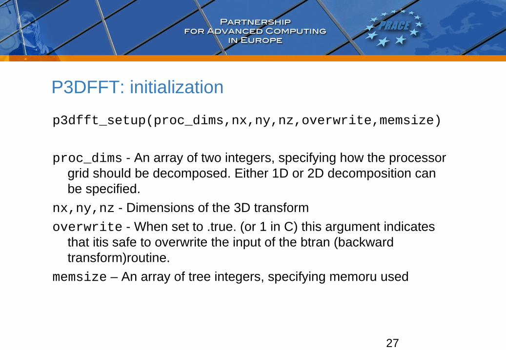
P3DFFT: initialization
p3dfft_setup(proc_dims,nx,ny,nz,overwrite,memsize)
proc_dims - An array of two integers, specifying how the processor grid should be decomposed. Either 1D or 2D decomposition can be specified.
nx,ny,nz - Dimensions of the 3D transform
overwrite - When set to .true. (or 1 in C) this argument indicates that itis safe to overwrite the input of the btran (backward transform)routine.
memsize – An array of tree integers, specifying memoru used

28
P3DFFT: Array Decomposition
p3dfft_get_dims(start,end,size,ip)
start - An array containing 3 integers, defining the beginning indices of the local array for the given task within the global grid
end - An array containing 3 integers, defining the ending indices of the local array within the global grid
size - An array containing 3 integers, defining the local array’s dimensions
ip - An integer argument specifying one of the two choices for array types (1 for forward, 2 for backward, 3 for in-place transform)
29
P3DFFT: Array Decomposition
P3DFFT uses 2D block decomposition to assign local arrays for each task. Let P
1 and P
2 be processor grid
dimensions defined in the call to p3dfft_setup.
For ip=1 Array is distributed among P1 tasks in Y
dimension and P2 tasks in Z dimension
For ip=2 Array is distributed among P1 tasks in X
dimension and P2 tasks in Y dimension
30
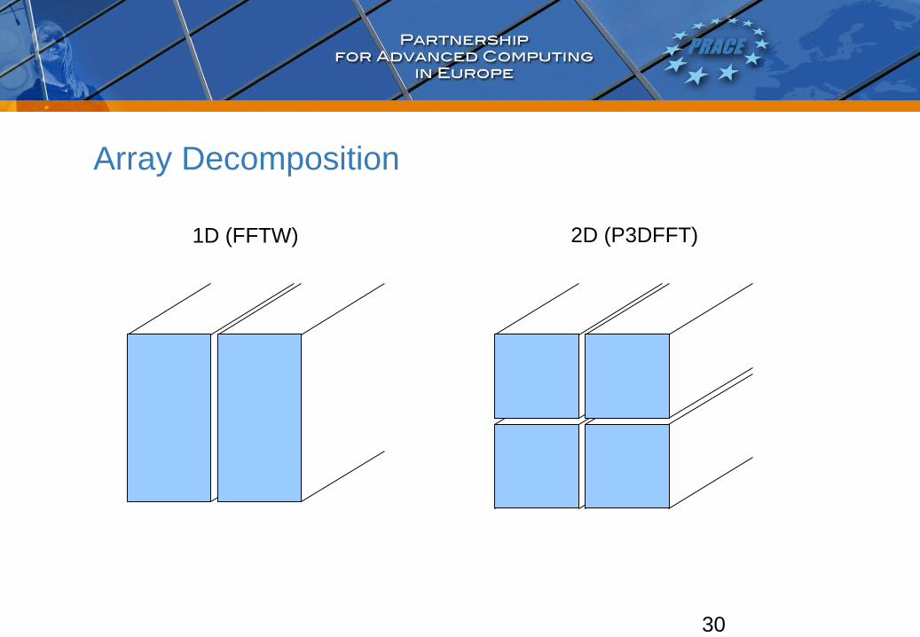
Array Decomposition
1D (FFTW) 2D (P3DFFT)
31
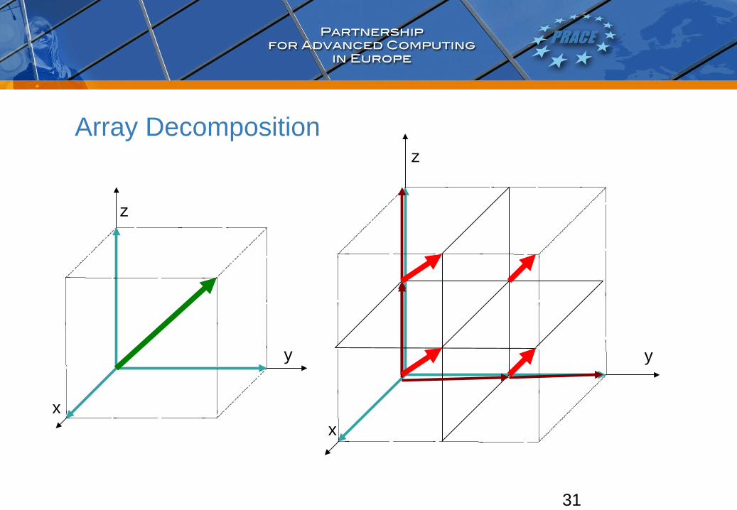
Array Decomposition
x
y
z
x
y
z
32
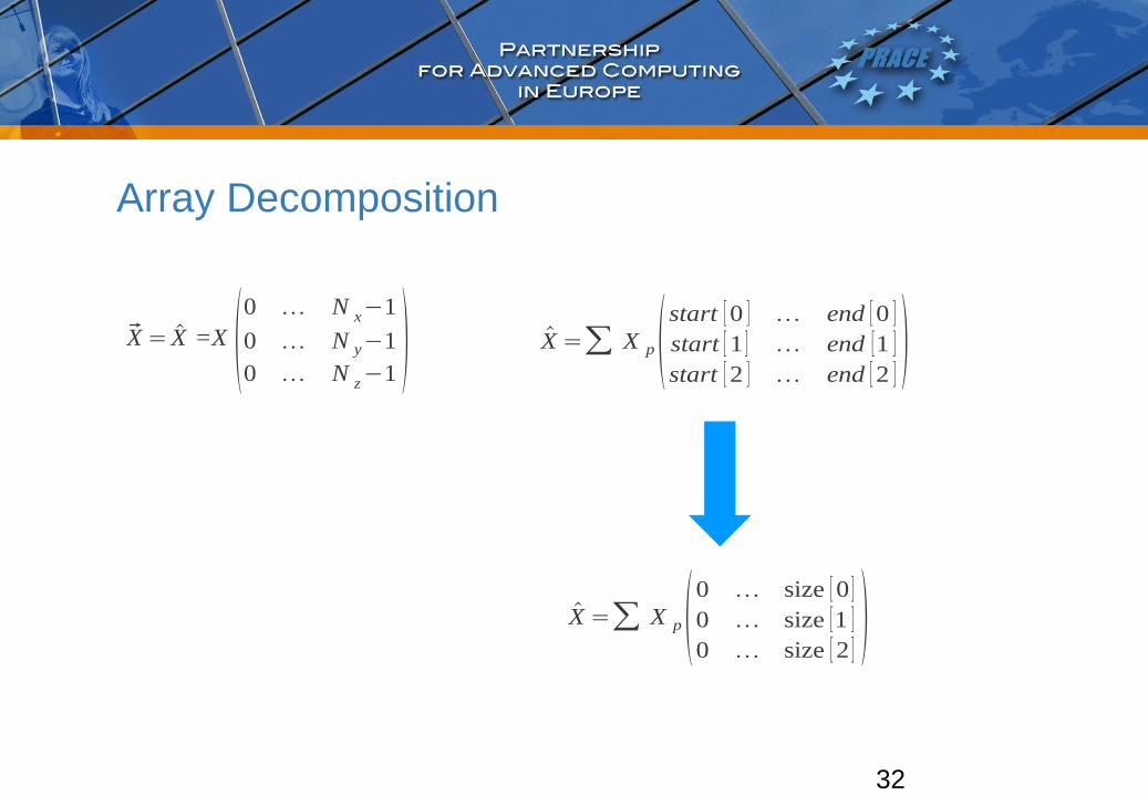
Array Decomposition
X = X =X 0 N x−1
0 N y−10 N z−1
X =∑ X p 0 size [0 ]0 size [1 ]0 size [2 ]
X =∑ X p start [0 ] end [0 ]start [1 ] end [1 ]start [2 ] end [2 ]
33
P3DFFT: Forward transform
p3dfft_ftran_r2c(IN,OUT,op)
IN - an array of real numbers with dimensions defined by array type with ip=1
OUT - an array of complex numbers with dimensions defined by array type with ip=2
op - 3-letter character string indicating the type of transform desired in X, Y, Z direction
t Fourier transform
c Cosine transform
s Sine transform
n or 0 Empty transform (no operation, output is identical to input)

34
P3DFFT: Forward transform
IN - an array of double numbers in order:
x
y
3
1
2
z
35
P3DFFT: Forward transform
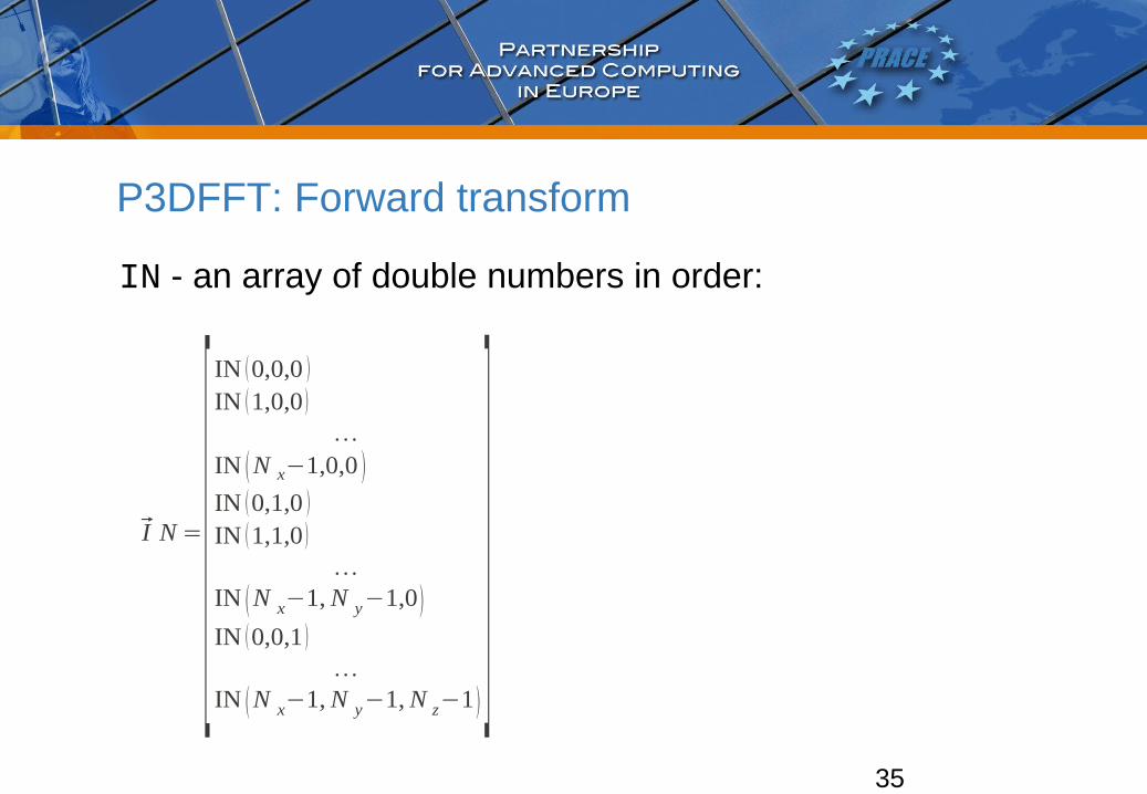
IN - an array of double numbers in order:
I N =[IN 0,0,0 IN 1,0,0
IN N x−1,0,0 IN 0,1,0 IN 1,1,0
IN N x−1,N y−1,0 IN 0,0,1
IN N x−1,N y−1,N z−1
]
36
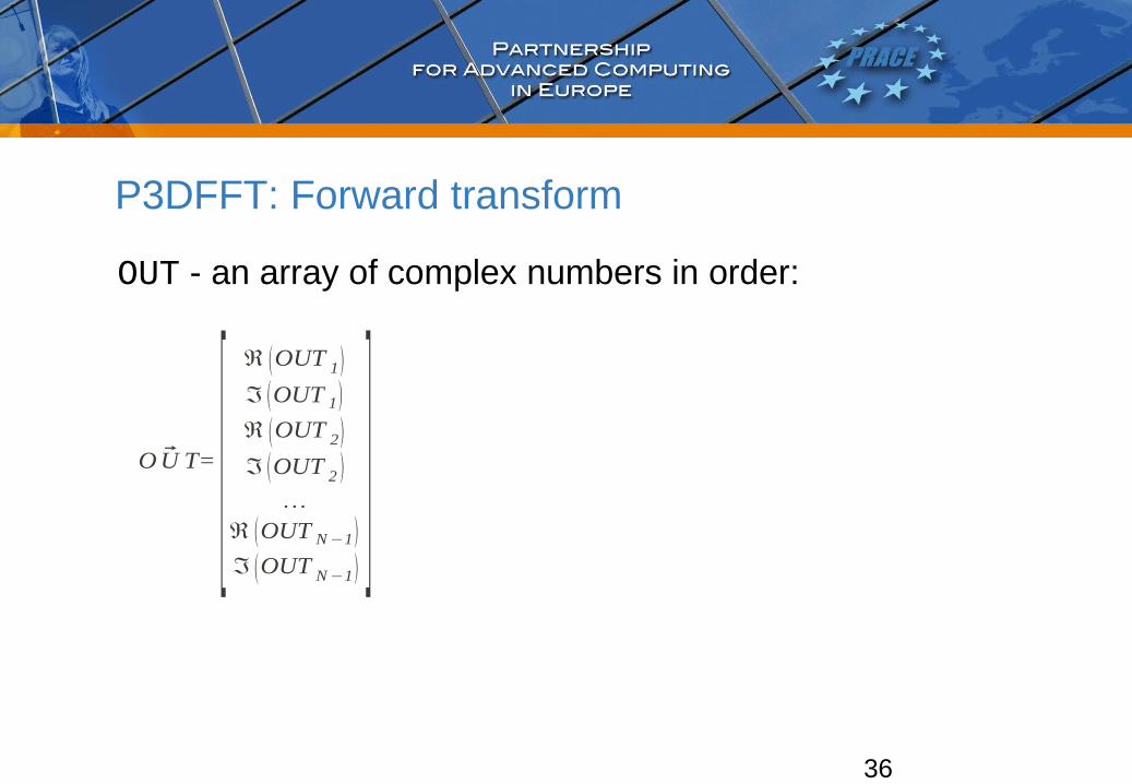
P3DFFT: Forward transform
OUT - an array of complex numbers in order:
O U T= [ℜ OUT 1ℑ OUT 1ℜ OUT 2ℑ OUT 2
ℜ OUT N−1ℑ OUT N−1
]
37
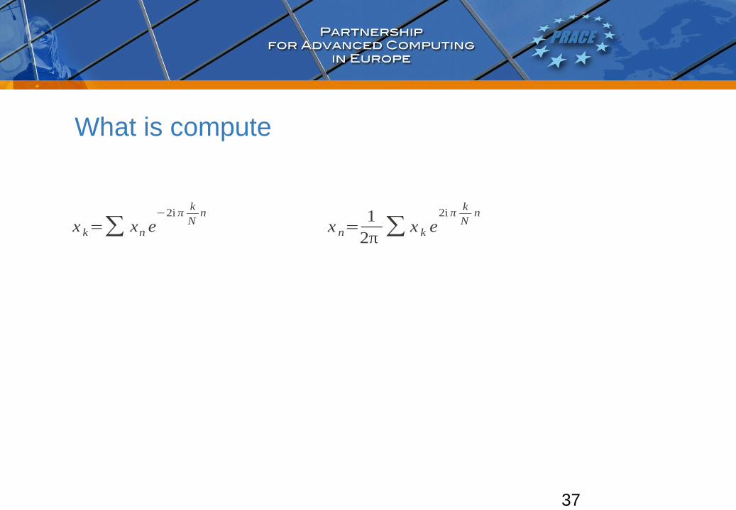
What is compute
x k=∑ xn e−2i π
kN
n
x n=1
2π∑ x k e
2i πkN
n

38
What is compute
x k=∑ xn e−2i π
kN
n
x n=1
2π∑ xk e
2i πkN
n
x nFFT xk
iFFT Nxn

39
P3DFFT: Backward transform
p3dfft_ftran_c2r(IN,OUT,op)
IN - an array of real numbers with dimensions defined by array type with ip=2
OUT - an array of complex numbers with dimensions defined by array type with ip=1
op - 3-letter character string indicating the type of transform desired in X, Y, Z direction
t Fourier transform
c Cosine transform
s Sine transform
n or 0 Empty transform (no operation, output is identical to input)
40
Terminates P3DFFT
p3dfft_clean() - Terminates P3DFFT