FFT-Based Algorithm for Metering Applicationscore of the radix-2 DIT FFT. Note, that final outputs...

Freescale SemiconductorApplication Note

Documents Number: AN4255Rev.1, 10/2013

Contents

Introduction . . . . . . . . . . . . . . . . . . . . . . . . . . . . . . . . . . . 1DFT basics. . . . . . . . . . . . . . . . . . . . . . . . . . . . . . . . . . . . 2FFT implementation . . . . . . . . . . . . . . . . . . . . . . . . . . . . . 2

3.1 The Radix-2 decimation in time FFT description . . . 33.2 The Radix-2 decimation in time FFT requirements . 63.3 The Radix-2 decimation in time FFT conclusion . . . 7Using an FFT for power computing . . . . . . . . . . . . . . . . . 8

4.1 Conversion between Cartesian and polar forms . . . 84.2 Root Mean Square computing . . . . . . . . . . . . . . . . . 94.3 Complex power computing . . . . . . . . . . . . . . . . . . . 9Practical implementation . . . . . . . . . . . . . . . . . . . . . . . . 11

5.1 API summary . . . . . . . . . . . . . . . . . . . . . . . . . . . . . 125.2 FFT_radix2 function. . . . . . . . . . . . . . . . . . . . . . . . 125.3 PowerCalculation function . . . . . . . . . . . . . . . . . . . 135.4 Computing performance . . . . . . . . . . . . . . . . . . . . 14Summary . . . . . . . . . . . . . . . . . . . . . . . . . . . . . . . . . . . . 14References. . . . . . . . . . . . . . . . . . . . . . . . . . . . . . . . . . . 14Revision history . . . . . . . . . . . . . . . . . . . . . . . . . . . . . . . 15

FFT-Based Algorithm for Metering Applicationsby: Luděk Šlosarčík

Rožnov Czech System CenterCzech Republic

1 IntroductionThe Fast Fourier Transform (FFT) is amathematical technique for transforming atime-domain digital signal into a frequency-domainrepresentation of the relative amplitude of differentfrequency regions in the signal. The Fast FourierTransform is a method for doing this process veryefficiently. The FFT may be computed using arelatively short excerpt from a signal.

The Fast Fourier Transform is one of the mostimportant topics in Digital Signal Processing. TheFFT is extremely important in the area of frequency(spectrum) analysis: for example, voice recognition,digital coding of acoustic signals for data streamreduction in the case of digital transmission,detection of machine vibration, signal filtration,solving partial differential equations, and so on.

This application note describes how to use the FFTin metering applications, especially for power andenergy computing in power meters.

123

4

5

678

© 2013 Freescale Semiconductor, Inc.

DFT basics

2 DFT basicsFor a proper understanding of the next sections, it is important to clarify what a Discrete FourierTransform (DFT) is. The DFT is a specific kind of discrete transform, used in Fourier analysis. Ittransforms one function into another, which is called the frequency domain representation of theoriginal function (a function in the time domain). The input to the DFT is a finite sequence of realor complex numbers, making the DFT ideal for processing information stored in computers. Therelationship between the DFT and the FFT is as follows: DFT refers to a mathematicaltransformation or function, regardless of how it is computed, whereas the FFT refers to a specificfamily of algorithms for computing a DFT.

The DFT of a finite-length sequence of size N is defined as follows:

Eqn. 1

Where:

X(k) is the output of the transformation

x(n) is the input of the transformation (the sampled input signal)

j is the imaginary unit

Each item in Equation 1 defines a partial sinusoidal element in complex format with a kF0frequency, with (2nk/N) phase, and with an x(n) amplitude. Their vector summation forn=0,1,...,N-1 (see Equation 1) and for the selected k-item, represents the total sinusoidal item ofspectrum X(k) in complex format for the kF0 frequency. Note, that F0 is the frequency of the inputperiodic signal. In the case of non-periodic signals, F0 means the selected basic period of thissignal for DFT computing.

The Inverse Discrete Fourier Transform (IDFT) is given by:

Eqn. 2

Thanks to Equation 2, it is possible to compute discrete values of x(n) retrospectively from thespectrum items of X(k).

In these two equations, both X(k) and x(n) can be complex, so N complex multiplications and(N-1) complex additions are required to compute each value of the DFT if we use Equation 1directly. Computing all N values of the frequency components requires a total of N2 complexmultiplications and N(N-1) complex additions.

3 FFT implementationWith regards to the derived equations in the previous chapter, it is good to introduce the followingsubstitution:

X k x n ej2nkN

-------------–

n 0=

N 1–

x n 2nkN

------------- cos j x n 2nk

N------------- sin–

n 0=

N 1–

= =0 k N

x n 1N---- X k e

j2nkN

-------------

k 0=

N 1–

= 0 n N

FFT-Based Algorithm for Metering Applications, Rev.1

Freescale Semiconductor, Inc.2

FFT implementation

Eqn. 3

The WNnk element in this substitution is also called the “twiddle factor”. With respect to this

substitution we may rewrite the equation for computing the DFT and IDFT into these formats:

Eqn. 4

Eqn. 5

To improve efficiency in computing the DFT, some properties of WNnk are exploited. They are

described as follows:

Symmetral property: Eqn. 6

Periodicity property: Eqn. 7

Recursion property: Eqn. 8

These properties arise from the graphical representation of the twiddle factor (Equation 3) by therotational vector for each nk value.

3.1 The Radix-2 decimation in time FFT description

The basic idea of the FFT is to decompose the DFT of a time domain sequence of length N intosuccessively smaller DFTs whose calculations require less arithmetic operations. This is knownas a divide-and-conquer strategy, one made possible by those properties described in theprevious section. Decomposition into shorter DFTs may be performed by splitting an N-pointinput data sequence x(n) into two N/2-point data sequences a(m) and b(m), corresponding to theeven-numbered and odd-numbered samples of x(n), respectively, that is:

• a(m) = x(2m), i.e. samples of x(n) for n=2m

• b(m) = x(2m+1), i.e. samples of x(n) for n=2m+1

where m is an integer ranging in 0m<N/2.

This process of splitting the time domain sequence into even and odd samples is what gives thealgorithm its name, “Decimation In Time (DIT)”. Thus, a(m) and b(m) are obtained by decimatingx(n) by a factor of 2; hence, the resulting FFT algorithm is also called “radix-2”. It is the simplestand most common form of the Cooley-Tukey algorithm [1].

WNnk

ej2nkN

-------------–

=

DFT x n X k x n WNnk

n 0=

N 1–

= =

IDFT X k x n 1N---- X k WN

n– k

k 0=

N 1–

= =

WNnk N 2+

W– Nnk

=

WNnk

WNnk N+

W= Nnk 2N+

= =

WN 2nk

WN2nk

=


Freescale Semiconductor, Inc. 3

FFT implementation

Now, the N-point DFT (see Equation 1) can be expressed in terms of DFTs of the decimated sequences as follows:

Eqn. 9

With the substitution given by Equation 8, the Equation 9 can be expressed as:

Eqn. 10

These two summations represent the N/2-point DFTs of the sequences a(m) and b(m),respectively. Thus, DFT[a(m)]=A(k) for even-numbered samples, and DFT[b(m)]=B(k) forodd-numbered samples. Thanks to the periodicity property (Equation 7) of the DFT, the outputsfor N/2k<N from a DFT of length N/2 are identical to the outputs for 0k<N/2. That is,A(k+N/2)=A(k) and B(k+N/2)=B(k) for 0k<N/2. In addition, the factor WN

k+N/2 = -WNk thanks the

to symmetral property (Equation 6).Thus, the whole DFT can be calculated as follows:

Eqn. 11

This result, expressing the DFT of length N recursively in terms of two DFTs of size N/2, is thecore of the radix-2 DIT FFT. Note, that final outputs of X(k) are obtained by a +/- combination ofA(k) and B(k)WN

k, which is simply a size 2 DFT. These combinations can be demonstrated by asimply oriented graph, sometimes called a “butterfly” in this context (see Figure 1).

Figure 1. Basic butterfly computation in the DIT FFT algorithm

The procedure of computing the discrete series of an N-point DFT into two N/2-point DFTs maybe adopted for computing the series of N/2-point DFTs from items of N/4-point DFTs. For thispurpose, each N/2-point sequence should be divided into two sub-sequences of even and odditems and computing their DFTs consecutively. The decimation of the data sequence can berepeated again and again until the resulting sequence is reduced to one basic DFT.

X k x n WNnk

n 0=

N 1–

x 2m WN2mk

m 0=

N 2 1–

x 2m 1+ WN2m 1+ k

m 0=

N 2 1–

+= = =

x 2m WN2mk

m 0=

N 2 1–

WNk

x 2m 1+ WN2mk

m 0=

N 2 1–

+=

X k a m WN 2mk

m 0=

N 2 1–

WNk

b m WN 2mk

m 0=

N 2 1–

+ A k WNkB k += = 0 k N

X k A k WNkB k += 0 k N 2

X k N 2+ A k WNk

– B k = 0 k N 2

A(k)

B(k)WN

k

X(k+N/2)=A(k)-WNkB(k)

X(k)=A(k)+WNkB(k)

-1



FFT implementation

Figure 2. Decomposition of an 8-point DFT

For illustrative purposes, Figure 2 depicts the computation of an N = 8-point DFT. We observethat computation is performed in three stages (3=log28), beginning with the computations of four2-point DFTs, then two 4-point DFTs, and finally, one 8-point DFT. Generally, for an N-point FFT,the FFT algorithm decomposes the DFT into log2N stages, each of which consist of N/2 butterflycomputations.The combination of the smaller DFTs to form the larger DFT is illustrated inFigure 3 for N=8.

Figure 3. 8-point radix-2 DIT FFT algorithm data flow

2-point

DFT

2-point

DFT

2-point

DFT

2-point

DFT

Combine2-point DFT’s



stage 1 stage 2 stage 3

X(0)X(1)X(2)X(3)

X(4)X(5)X(6)X(7)

x(4)

x(2)x(6)

x(1)

x(5)

x(3)x(7)

x(0)

x(0)

x(4)W8

0

x(2)

x(6)W8

0

x(1)

x(5)W8

0

x(3)

x(7)W8

0 W82

W82

W80

W80

W80

W81

W82

W83

-1-1

-1

-1

-1

-1

-1

-1

-1

-1

-1

-1

X(0)

X(1)

X(2)

X(3)

X(4)

X(5)

X(6)

X(7)

stage 3stage 2stage 1

x(n) X(k)

k=0 k=0,1 k=0,1,2,3

W84k=W2

k W82k=W4

k W8k



FFT implementation

Note, that each dot represents a complex addition and each arrow represents a complexmultiplication in Figure 3. The WN

k factors in Figure 3 may be presented as a power of two (W2)at the first stage, as a power of four (W4) at the second stage, as a power of eight (W8) at thethird stage, etc. It is also possible to represent it uniformly as a power of N (WN ), where N is thesize of the input sequence x(n). Context between both of these expressions gives Equation 8.

3.2 The Radix-2 decimation in time FFT requirements

For effective and optimal decomposition of the input data sequence into even and oddsub-sequences, it is good to have the power-of-two input data samples (...,64,128, and so on).

The first step before computing the radix-2 FFT is a re-ordering of the input data sequence (seealso the left side of Figure 2 or Figure 3). This means that this algorithm needs a bit-reverseddata ordering; that is, the MSBs become LSBs, and vice versa. Table 1 shows an example ofbit-reversal with an 8-point input sequence.

It is important to note that this type of FFT algorithm is an “in place”, which means that the outputsof each butterfly throughout the computation can be placed in the same memory locations fromwhich the inputs were fetched, resulting in an in-place algorithm that requires no extra memoryto perform the FFT.

3.2.1 Window selection

The FFT computation assumes that a signal is periodic in each data block; that is, it repeats overand over again. Most signals aren’t periodic, and even a periodic one might have an unknownperiod. When the FFT of a non-periodic signal is computed, then the resulting frequencyspectrum suffers from leakage. To resolve this issue, it is good to take N samples of the inputsignal and make them periodic. This may be generally performed by window functions (Barlett,Blackman, Kaiser-Bessel, and so on). Considering that the resulting spectrum after theapplication of some window function may have a slightly different shape in comparison to thefrequency spectrum of a pure periodic signal without windowing, it is better not to use a specialwindow function in a metering application too, or to use a simple rectangular window (a functionwith a coherent gain of 1.0). This requires that the frequency of the input signal is well known, ofcourse. In metering applications, this is accomplished thanks to measuring a period of linevoltage.

The detection of a signal (mains) period may be performed by a zero-cross detection (ZCD)technique. Zero-crossing is the instantaneous point at which there is no voltage present (seeFigure 4a). In a line voltage wave, or other simple waveform, this normally occurs twice duringeach cycle. Counting the zero-crossing is a method used for frequency measurement of an input

Table 1. Bit reversal with an 8-point input sequence

Decimal number 0 1 2 3 4 5 6 7

Binary equivalent 000 001 010 011 100 101 110 111

Bit reversed binary 000 100 010 110 001 101 011 111

Decimal equivalent 0 4 2 6 1 5 3 7



FFT implementation

signal (the line voltage). For example, the ZCD circuit may be realized by using an analoguecomparator inside the MCU, where the first channel is connected to the reference voltage andthe second channel is connected to the line through a simple voltage divider. Finally, the changein logic level from this comparator is interpreted by software as a zero-crossing of the mains. Thetime between zero-crossings is measured by a timer in the software. These zero-crossings alsodefine the start and end-points of a simple rectangular FFT window (Figure 4a). Technically, it isnot necessary to measure the frequency of an input signal by zero-cross points, but it is possibleto use any other two points of the input signal that may be simply recognized - peak points, forexample (see Figure 4b) - with a similar result (magnitudes are the same, phases are uniformlyshifted).

Figure 4. Zero-cross point vs. peak point detection

It is also good to know that this software technique for measuring the signal frequency mustcontain some kind of sophisticated algorithm for removing possible voltage spikes (see Figure 4).These spikes may appear in the line as a product of interference from a load (motor, contactor,and so on) and may cause false zero-crossing or peak detection.

In a practical implementation, it is better to measure the time between several true zero-cross orpeak points. Finally, an arithmetic mean must be performed to compute the correct signalfrequency. Each period of input signals (voltage and current) is then sampled with a frequency,which is N times higher than the measured frequency of the line voltage, where N is the numberof samples. When the sampling frequency is different from this, the resulting frequency spectrummay suffer from leakage.

3.3 The Radix-2 decimation in time FFT conclusion

The radix-2 FFT utilizes some clever algorithms to do the same thing as the DFT, but in muchless time. Whereas the DFT needs N2 complex multiplications (see at Section 2, “DFT basics),the FFT takes only N/2log2N complex multiplications and Nlog2N complex additions. Therefore,

a b



Using an FFT for power computing

the ratio between the DFT computation and the FFT computation for the same N is proportionalto 2N / log2N. In cases where N is small, this ratio is not very significant, but when N becomeslarge, this ratio gets very large. Therefore, the FFT is simply a fast way to calculate the DFT.

The radix-2 FFT algorithm is generally defined as a radix-r FFT algorithm, where the N-pointinput sequence is split into r-subsequences to raise computation efficiency, for example radix-4or radix-8. Thus, the radix is the size of the FFT decomposition.

Similarly the DIT algorithm is sometimes used Decimation In Frequency (DIF) algorithm (alsocalled the Sande-Tukey algorithm), which decomposes the sequence of DFT coefficients X(k)into successively smaller sub-sequences[3]. However, this application note describes only theradix-2 DIT FFT algorithm.

4 Using an FFT for power computing

4.1 Conversion between Cartesian and polar forms

The FFT implementation in power meters requires complex number computing, because themathematical formulas describing the DFT or FFT in previous chapters suppose that each itemin these formulas (in graphical format these are X(k) in Figure 3) contains a complex number.

A complex number is a number consisting of a real and an imaginary part. This number can berepresented as a point or position vector in a two-dimensional Cartesian coordinate systemcalled the complex plane. The numbers are conventionally plotted using the real part as thehorizontal component, and imaginary part as the vertical (see Figure 5).

Figure 5. A graphical representation of a complex number

Another way of encoding points in the complex plane, other than using the x- and y-coordinates,is to use the distance of a point z to O, the point whose coordinates are (0,0), and the angle ofthe line through z and O. This idea leads to the polar form of complex numbers. The absolutevalue (or magnitude) of a complex number z=x+iy is

Eqn. 12

The argument or phase of z is defined as:

Eqn. 13

r z x2y

2+= =

z argyx-- atan= =




Together, r and show another way of representing complex numbers, the polar form, as thecombination of modulus and argument fully specify the position of a point on the plane.

4.2 Root Mean Square computing

In electrical engineering, the Root Mean Square (RMS) is a fundamental measurement of themagnitude of an AC signal. The RMS value assigned to an AC signal is the amount of DCrequired to produce an equivalent amount of heat in the same load. In a complex plane, the RMSvalue of the current (IRMS) and the voltage (URMS) is the same as the summation of theirmagnitudes (see vector r in Figure 5) associated for each harmonic. Regarding Equation 12, thetotal RMS values of current and voltage in the frequency domain are defined as:

Eqn. 14

Where:

IRE(k), URE(k) are real parts of kth harmonics of current and voltage.

IIM(k), UIM(k) are imaginary parts of kth harmonics of current and voltage.

4.3 Complex power computing

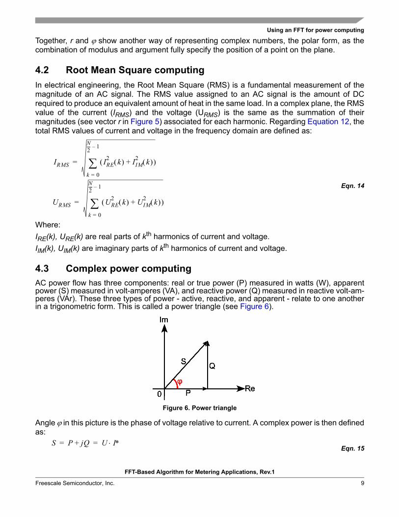
AC power flow has three components: real or true power (P) measured in watts (W), apparentpower (S) measured in volt-amperes (VA), and reactive power (Q) measured in reactive volt-am-peres (VAr). These three types of power - active, reactive, and apparent - relate to one anotherin a trigonometric form. This is called a power triangle (see Figure 6).

Figure 6. Power triangle

Anglein this picture is the phase of voltage relative to current. A complex power is then definedas:

Eqn. 15

IRMS IRE2k IIM

2k +

k 0=

N2---- 1–

=

URMS URE2k UIM

2k +

k 0=

N2---- 1–

=

S P jQ+ U I= =




Where U is a voltage vector (U=URE+jUIM) and I is a current vector (I=IRE+jIIM). Note, that I* is acomplex conjugate current vector.

Regarding Equation 12, the length of a complex power (|S|) is the apparent power (VA) actually.In terms of current and voltage phasors (FFT outputs), and in terms of Equation 15, the complexpower in Cartesian form can be finally expressed as:

Eqn. 16

Where:

IRE(k), URE(k) are real parts of kth harmonics of current and voltage.

IIM(k), UIM(k) are imaginary parts of kth harmonics of current and voltage.

In terms of Equation 12 and Equation 13, both parts of the total complex power (P and Q) can bealso expressed in polar form as:

Eqn. 17

Where:

|I(k)|, |U(k)| are magnitudes of kth harmonics of current and voltage.

I(k), U(k) are phase shifts of kth harmonics of current and voltage (with regards to the FFTwindow origin).

Note, that inputs for these equations are Fourier items of current and voltage (in Cartesian orpolar form). For a graphical interpretation of these items, see X(k) in Figure 3.

There are two basic simplifications used in the previous formulas:

• Thanks to the symmetry of the FFT spectrum, only N/2 items are used for complex powercomputing.

• It is expected that voltage in the mains has no DC offset. Therefore the 0-harmonic ismissed in both formulas because of multiplication of the current values (IRE(0), IIM(0),|I(0)|) with zero.

Total apparent power may be also computed from the RMS values of voltage and current as:

S URE k jUIM k + IRE k jIIM– k

k 1=

N2---- 1–

= =

IRE k URE k IIM k UIM k + j UIM k IRE k URE k IIM k – +

k 1=

N2---- 1–

=

real part of complex power imaginary part of complex power

S I k U k U k I k – cos j I k U k U k I k – sin +

k 1=

N2---- 1–

=

real part of complex power imaginary part of complex power



Practical implementation

Eqn. 18

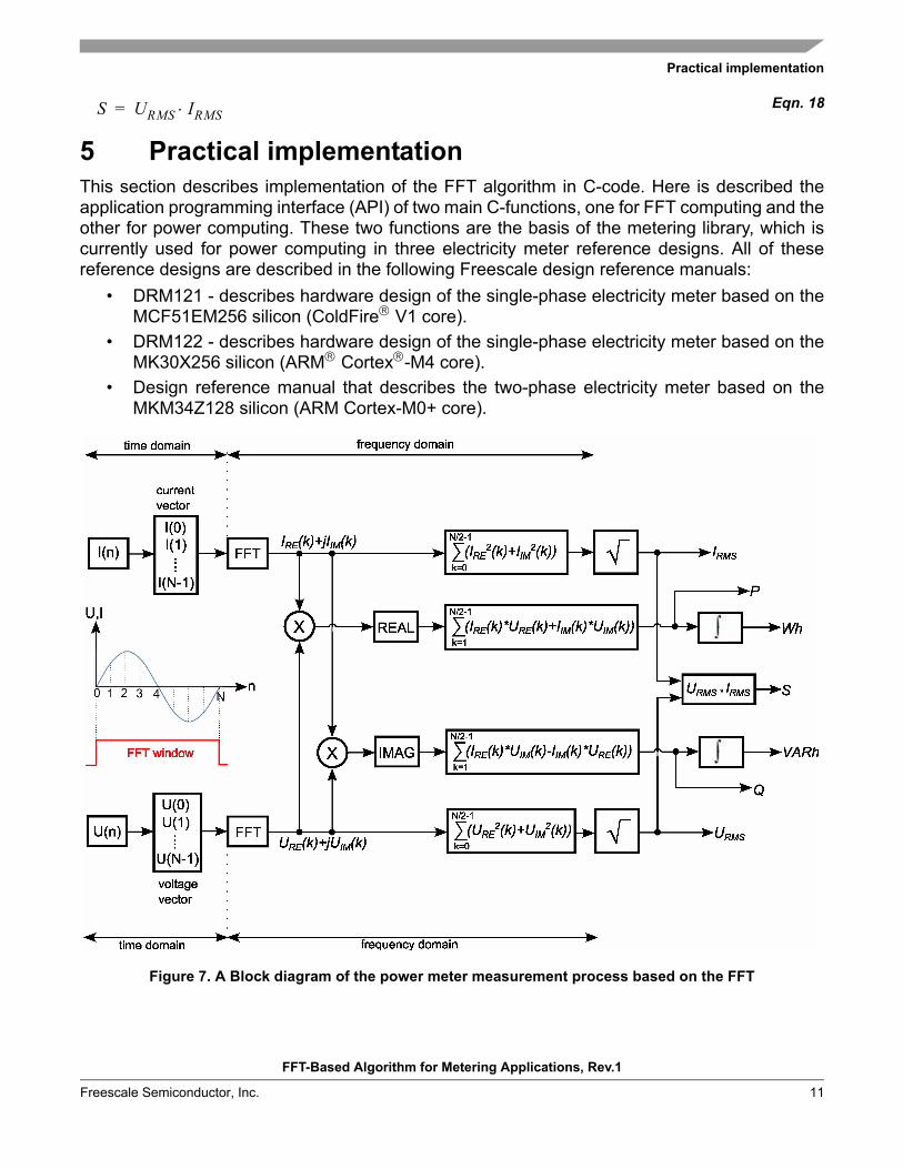
5 Practical implementationThis section describes implementation of the FFT algorithm in C-code. Here is described theapplication programming interface (API) of two main C-functions, one for FFT computing and theother for power computing. These two functions are the basis of the metering library, which iscurrently used for power computing in three electricity meter reference designs. All of thesereference designs are described in the following Freescale design reference manuals:

• DRM121 - describes hardware design of the single-phase electricity meter based on theMCF51EM256 silicon (ColdFire V1 core).

• DRM122 - describes hardware design of the single-phase electricity meter based on theMK30X256 silicon (ARM Cortex-M4 core).

• Design reference manual that describes the two-phase electricity meter based on theMKM34Z128 silicon (ARM Cortex-M0+ core).

Figure 7. A Block diagram of the power meter measurement process based on the FFT

S URMS IRMS=




In true power meters, the energies (active, reactive) are computed from the powersconsecutively by accumulation of these powers per time unit. A simple block diagram of thiscomputing process in a typical power meter is depicted in Figure 7.

5.1 API summary

This section describes the application programming interface (API) used in the metering library.There are defined two main functions (see Table 2) in the metering library: FFT_radix2 andPowerCalculation. There are also some additional mathematical functions used inside thesemain functions, such fractional, radix and arctangent computing functions.

1) Valid for ARM Cortex-M0+ core.

5.2 FFT_radix2 function

This function computes the FFT of the input signal: that is, it transforms input data from the timedomain into the frequency domain using the radix-2 DIT algorithm (see Section 3.1, “The Radix-2decimation in time FFT description). The output parameters (arguments) from this function arein Cartesian data format. Each real and imaginary item of the output spectrum has a width of 32bits.

5.2.1 Synopsis

This subsection provides the header file that should be included within a source file thatreferences the FFT_radix2 function. An appropriate declaration for this function is also shownbelow. This declaration is not included in your program; only the header file should be included:

#include “fft2.h”

void FFT_radix2(unsigned short n,long input[N_SAMPLES],ComplexFFT result[N_SAMPLES])

5.2.2 Arguments

This subsection describes input and output arguments of the FFT_radix2 function.

Table 2. API functions summary

Name Arguments Output Description Code size1)

FFT_radix2 n, input, result void Computes the FFT (radix-2 DIT algorithm) 514 bytes

PowerCalculation voltage, current, powers, mU,mI void Computes the whole power vector 706 bytes

Table 3. FFT_radix2 function arguments

Name In/Out Data format Used range Description

n In unsigned 16-bits 8, 16, 32, 64, 128 Number of samples per one period of input signal

input In signed 32-bits 0x80000000 ... 0x7FFFFFFF Input data buffer (size n) in time domain

result Out ComplexFFT see Table 4 Output data buffer (size n) in frequency domain




5.3 PowerCalculation function

This function computes the complete power vector of the input signal from the frequencyspectrum. The power vector contains these values: RMS value of the voltage, powers (active,reactive, apparent), and angle between the 1st harmonics of the current and voltage. ThePowerCalculation function calls internally the FFT_radix2 function two times, because it needsthe output arguments (spectrum) from both the channels, voltage and current channel.

5.3.1 Synopsis

This subsection provides the header file that should be included within a source file thatreferences the PowerCalculation function. There is also shown an appropriate declaration for thisfunction. This declaration is not included in your program; only the header file should be included:

#include “metering2.h”

void PowerCalculation (long voltage[N_SAMPLES], long current[N_SAMPLES], Power_Vector *powers, unsigned long mU[MAX_FFT_SEND], unsigned long mI[MAX_FFT_SEND])

5.3.2 Arguments

This subsection describes input and output arguments of the PowerCalculation function.

Table 4. ComplexFFT data type definition

Name Data format Range Description

Real signed 32-bits 0x80000000 ... 0x7FFFFFFF Integer part of each real item (Cartesian form)

Img signed 32-bits 0x80000000 ... 0x7FFFFFFF Integer part of each imaginary item (Cartesian form)

Table 5. PowerCalculation function arguments

Name In/Out Data format Used range Description

voltage In signed 32-bits 0x80000000 ... 0x7FFFFFFF Voltage input data buffer (size n) in frequency domain

current In signed 32-bits 0x80000000 ... 0x7FFFFFFF Current input data buffer (size n) in frequency domain

powers Out Power_Vector see Table 6 Power vector (W, VAr, VA, VRMS, angle)

mU Out unsigned 32-bits 0x00000000 ... 0xFFFFFFFF Voltage magnitudes (used only for FreeMASTER visualization)

mI Out unsigned 32-bits 0x00000000 ... 0xFFFFFFFF Current magnitudes (used only for FreeMASTER visualization)

Table 6. Power_Vector data type definition

Name Data format Range Description

P signed 64-bits 0x8000000000000000 ... 0x7FFFFFFFFFFFFFFF Active power (not scaled)

Q signed 64-bits 0x8000000000000000 ... 0x7FFFFFFFFFFFFFFF Reactive power (not scaled)

S unsigned 64-bits 0x0000000000000000 ... 0xFFFFFFFFFFFFFFFF Apparent power (not scaled)

U unsigned 32-bits 0x00000000 ... 0xFFFFFFFF RMS value of voltage (not scaled)

Angle signed 32-bits 0x80000000 ... 0x7FFFFFFF Angle between the 1st harmonic of U and I



Summary

5.4 Computing performance

The metering library based on the FFT can be used with different hardware platforms (MCUs).This answers the MCU computational requirements for using this metering library on the ARMCortex-M0+ core (MKM34Z128 MCU). Table 7 shows computational time for PowerCalculationfunction, which calls the FFT_radix2 function two times, once for voltage FFT computation andthen for current FFT computation.

1) CPUCLK=47.972352 MHz, Compiler optimization=high speed, finp=50 Hz, Cartesian form of the FFT, ARM Cortex-M0+ core.

6 SummaryThis application note describes how to compute powers in a metering application using the FFT.A computing technique based on the FFT has some advantages and also disadvantages:

Advantages of realization:

• The same precision for both active and reactive energies

• Four quadrant active and reactive energy measurement

• Frequency analysis of the mains, ability to compute Total Harmonic Distortion (THD)

• Offset removal, because the 0-harmonic may be missed out for power computing

Disadvantages of realization:

• Adjustable sampling rate is necessary to compensate for the frequency changes in the mains

• Higher computational power of the MCU (a 32-bit MAC unit is required)

7 References[1] J.W.Cooley and J.W.Tukey, An algorithm for the machine calculation of the complex Fourier series, Math. Comp., Vol. 19 (1965), pp. 297-301

[2] Wikipedia articles “Cooley-Tukey FFT algorithm”, “Complex number”, “AC Power”, available at en.wikipedia.org

[3] AN2768, “Implementation of a 128-Point FFT on the MRC6011 Device”, available at freescale.com

Table 7. Computing performance of the whole FFT metering library

Number of FFT samples Computing time1) [ms] MCU execution cycles1)

8 0.24 11513

16 0.55 26384

32 1.13 54208

64 2.42 116093

128 5.36 257131



http://www.freescale.com/webapp/sps/site/prod_summary.jsp?code=S08JM&fsrch=1

http://www.freescale.com/


http://en.wikipedia.org/wiki/Main_Page

Revision history

[4] Fast Fourier Transform (FFT) article, available at http://www.cmlab.csie.ntu.edu.tw/cml/dsp/training/coding/transform/fft.html

[5] DRM121, “MQX-enabled MCF51EM256 Single-Phase Electricity Meter Reference Design”, available at freescale.com

[6] DRM122, “MQX-enabled MK30X256 Single-Phase Electricity Meter Reference Design”, available at freescale.com

8 Revision historyRevision number Date Substantial changes

0 11/2011 Initial release

1 10/2013 Upgrade Section 5, “Practical implementation





How to Reach Us:

Home Page:www.freescale.com

Web Support:freescale.com/support

Information in this document is provided solely to enable system and software implementers to use Freescale Semiconductor products. There are no express or implied copyright licenses granted hereunder to design or fabricate any integrated circuits or integrated circuits based on the information in this document.

Freescale reserves the right to make changes without further notice to any products herein. Freescale makes no warranty, representation, or guarantee regarding the suitability of its products for any particular purpose, nor does Freescale assume any liability arising out of the application or use of any product or circuit, and specifically disclaims any and all liability, including without limitation consequential or incidental damages. “Typical” parameters that may be provided in Freescale data sheets and/or specifications can and do vary in different applications, and actual performance may vary over time. All operating parameters, including “typicals,” must be validated for each customer application by customer’s technical experts. Freescale does not convey any license under its patent rights nor the rights of others. Freescale sells products pursuant to standard terms and conditions of sale, which can be found at the following address: freescale.com/SalesTermsandConditions.

Freescale, the Freescale logo, and Kinetis are trademarks of Freescale Semiconductor, Inc., Reg. U.S. Pat. & Tm. Off. All other product or service names are the property of their respective owners. ARM is the registered trademarks of ARM Limited. ARM Cortex-M0+ is the trademark of ARM Limited.

© 2013 Freescale Semiconductor, Inc. All rights reserved.

Documents Number: AN4255Rev. 110/2013

Documents Number: AN4255Rev. 110/2013




FFT-Based Algorithm for Metering Applicationscore of the radix-2 DIT FFT. Note, that final outputs...

Documents

Transcript of FFT-Based Algorithm for Metering Applicationscore of the radix-2 DIT FFT. Note, that final outputs...