Western Region Technical Attachment No. 94-02

December 11, 1993

USING PCGRIDS TO FORECAST SYl.\11\ffiTRIC INSTABILITY IN A NORTHEAST COLORADO SNOWSTORM

Introduction

Michael C. Conger and Lawrence B. Dunn WSFO Salt Lake City

During the late afternoon and evening of 28 October 1993, widespread snowfall developed over northeast Colorado. Two distinct areas of heavy snow were observed in: 1) the upslope zone of the Colorado Front Range; and 2) bands extending west-east away from the Front Range. Classic orographic influences explain the heavy snow in the upslope zone. However, in the banded heavy snow pattern, topography was not a direct factor. A probable explanation for the banded heavy snow would be slantwise convection due to conditional symmetric instability (CST).

Historically, there have been two major problems associated with banded precipitation in the operational environment. The first is associated with the difficulty of conventional radar in observing th e bands during winter. Often mesoscale snow bands simply do not show up in WSR-57 or WSR-74 radar data. Installation of the WSR-88D, having significantly higher resolution and sensitivity, has greatly improved this situation. Forecast offices can expect to see mesoscale snow bands within most winter storms using the WSR-88D.

Forecasting these mesoscale precipitation bands is the second problem associated with banded precipitation in the operational environment. In most cases, this is still not possible. However, in the case of CSI, a theoretical framework exists to explain one type of mesoscale banding. Until recently, CSI could only be identified by creating cross-sections from upper-air observations. This t echnique has a number of problems, notably timeliness and poor spatial resolution. Gridded model output offers solutions to these drawbacks, with both prognostic information and high spatial resolution. This Technical Attachment illustrates methods for using gridded model output to identify areas of CSI in an operational setting.

Explanation and Example of CSI

A number of articles exist on the subject of CSI. Emanuel (1983) addresses the mathematics behind the CSI theory. Sanders and Bosart (1985) and Bennetts et al. (1988) explain the process in simpler terms. Lussky (1987) discussed the operational use of CSI diagnosis from upper-air observations for a heavy rain/ flood event in eastern Montana. Dunn (1988)

presented a case study of CSI in a heavy snow event over eastern Colorado with synoptic-scale conditions very similar to the case examined here. Although the latter two papers were operationally oriented, their use of observations to diagnose CSI is very difficult to do in real time.

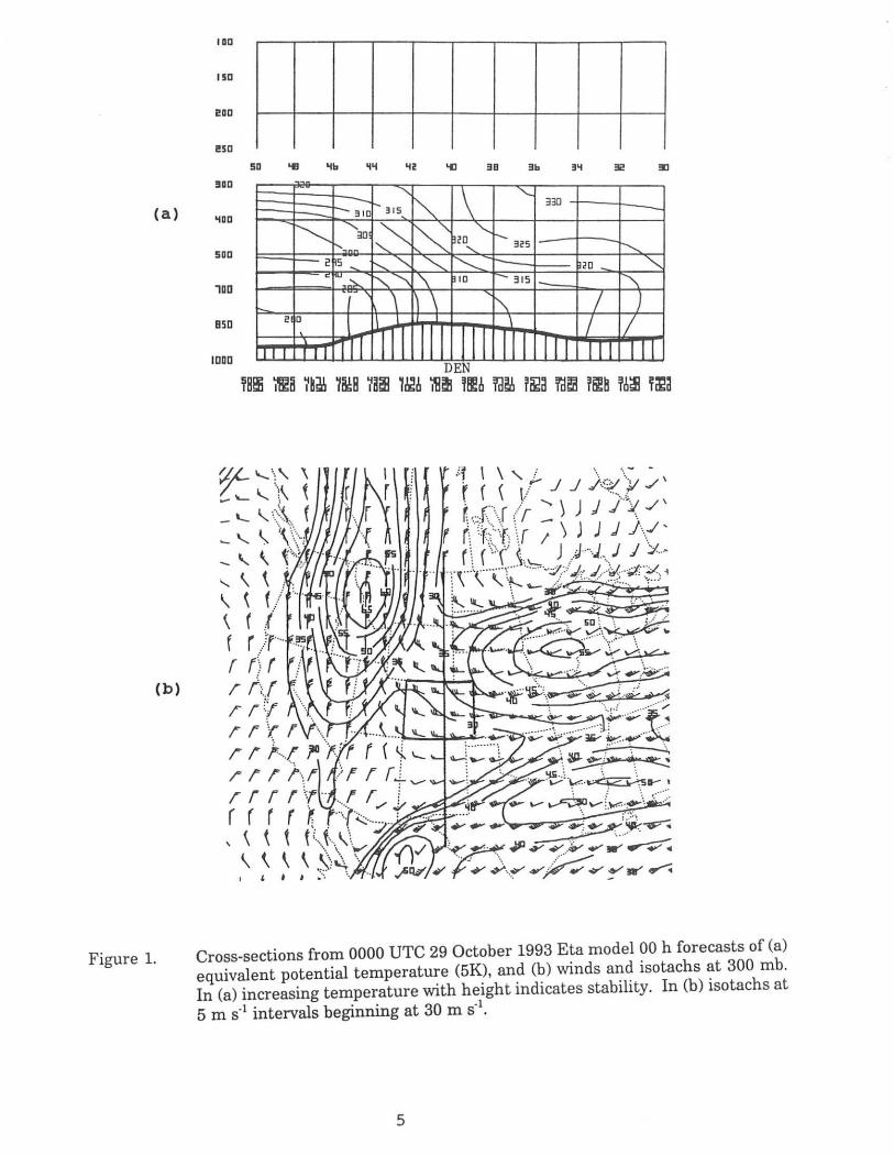
For CSI to exist, three conditions must be considered: vertical stability, inertial stability, and sufficient moisture. In cases of CSI, the air mass must be slightly convectively stable or neutral to vertical ascent (else, upright convection would exist) and have weak inertial stability (stability with respect to horizontal displacement). As defined in Holton (1992), the flow is inertially stable when the absolute vorticity is positive. In extratropical synoptic-scale systems, the flow is always inertially stable, although near neutrality (i.e., weak inertial stability) occurs on the anticyclonic shear side of upper-level jet streaks. Around the time of heavy snow (0000 UTC), a cross-section of equivalent potential temperature ( E> e) through northeast Colorado (50-30° N along 105° W) from the Eta model 00 h forecast (Fig. 1a) shows a slightly stable air mass. At the same time, northeast Colorado was under the anticyclonic shear side of the upper-level jet streak (Fig. 1b). Saturation or near saturation is necessary in regions of CSI to support heavy precipitation (later figures will show the air mass is near saturation over northeast Colorado during the snow event).

CSI is determined by examining the forcing of a parcel both in the vertical and horizontal. This process is done along surfaces of constant momentum. Momentum (M) is defined by Emanuel (1983) as, M = vg + fx, where vg is the geostrophic component of the flow normal to the cross-section, f is the Coriolis parameter, and x the distance along the cross-section. Diagnosis of CSI is done by constructing a cross-section of M-surfaces, ee, and relative humidity (RH), oriented normal to the thermal wind (thickness lines). As stated by Lussky (1987), the atmosphere exhibits CSI in regions where ee decreases following a parcel's ascent along an M-surface, (i.e. ee contours are steeper than M-surfaces). Also, if a parcel travels a slantwise path such that ee does not increase and M does not decrease (ee and M-surfaces are parallel), then a parcel has encountered CSI and is unstable along a slantwise path while being stable to vertical and horizontal displacement separately.

Prior to the availability of gridded data at field offices, no suitable method existed to forecast CSI. Now, using gridded data with graphics produced from PCGRIDS software, cross-sections of CSI can be produced at 6 h intervals through 48 h. In this study, both the Eta model and Nested Grid Model (NGM) were quite similar. For the sake of brevity, only the Eta model will be used to illustrate the points in this article.

Using the method described to locate CSI, the 12 h forecast from the Eta model (1200 UTC 28 October 1993, valid 0000 UTC 29 October 1993) (Fig. 2a) clearly shows an area favorable for CSI through a substantial depth of the atmosphere over northeast Colorado. The 00 h forecast valid 0000 UTC 29 October 1993 (Fig. 2b), locates an area of CSI corresponding well with the 12 h forecast valid at the same time.

Two reflectivity images at a 0.5 degree elevation angle from the Front Range WSR-88D are shown in Figs. 3a-b. The two images are about two hours apart, and represent the near steady state conditions which existed in the reflectivity imagery between 0000-0500 UTC. A cold front had dropped south through eastern Colorado earlier in the day. West-east oriented bands of snow developed in the post-frontal region over northeast Colorado. The bands persisted for 5-6 hours with a general southward drift after formation. New bands formed

2

during this period farther north near the Wyoming/ Colorado border. Snowfall accumulations within the bands ranged from 6-11 inches.

Conclusion

One theory that might explain the heavy banded precipitation is slantwise convection due to conditional symmetric instability (CSI). Identifying this phenomena is difficult on conventional weather radar, and nearly impossible to forecast using traditional prognostic data in the operational environment. This has changed with the advent of the WSR-88D and the availability of gridded data to the field offices.

Doppler radar imagery and forecast products generated from gridded data using PCGRIDS software strongly support the possibility that CSI was the cause of heavy banded snowfall over northeast Colorado on 28 October 1993. However, a more important point this case illustrates is the ability of the forecaster to use the new tools to evaluate theory (in this case CSI) and apply that theory to real-time weather events. This greater flexibility afforded to the forecaster by the new technology can only help improve forecasting of both routine and extreme weather events.

Author's Note: The radar imagery used in this case was collected from the non-associated PUP at the CBRFC collocated with the WSFO Salt Lake City. This case study was not written to highlight a particular forecast, but to show the utility of the PCGRIDS software. In this case, conditional symmetric instability (CSI) was the topic, though many other theories previously ignored could be explored using the gridded data now available to field offices.

APPENDIX

The commands in PCGRIDS to produce 0c (THTE) and relative humidity (RELH) are straight forward. Momentum is computed using the following command string:

SSUM NORM GEOS SMLT FFFF DIST

where DIST is the distance along the cross-section and FFFF is the Coriolis parameter. When creating the cross-section, be sure it is normal to the thermal wind (thickness lines) at the point of interest. Also, the left most latitude/longitude pair in the XSCT command must be on the cold air side where DIST=O.

REFERENCES

Bennetts, D. A, J . R. Grant and E . McCallum, 1988: An introductory review of fronts. Part I: Theory and observations. Met. Mag. , 117, 357-371.

Dunn, L. B., 1988: Vertical motion evaluation of a Colorado snowstorm from a synoptician's perspective. Wea. Forecasting, 3, 261-272.

3

Emanuel, K. A., 1983: The lagrangian parcel dynamics of moist symmetric instability. J. Atmos. Sci., 40, 2368-2376.

Holton, J. R. , 1992: An Introduction to Dynamic Meteorology. 3rd ed., Int. Geophys. Ser., 48, Academic Press, 511 pp.

Lussky, G. R., 1987: Heavy rains and flooding in Montana: A case for slantwise convection. NOAA Technical Memorandum NWS WR-199.

Sanders, F. and L. F. Bosart, 1985: Mesoscale structure in the megalopolitan snowstorm of 11-12 February 1983. Part I: Frontogenetical forcing and symmetric instability. J. Atmos. Sci., 42, 1050-1061.

4

(a)

(b)

Figure 1.

IDO

ISO

I! DO

i!SO

SD 'I! 'ib ~'i 'i~ 'II 3B 3b 3ii!

5DO ~ -..... " \ "-

t-- 310 f-.. 315 ~ 330 --~ '3o i0 ~ w'-~ 3~5

'~"" -, ~

2 5 ..... '" """ '--...._ 1-- 20

"""

'iDO

500

"i<U ~ -......_"\ \ 10 - 315 - ""\ ...._ \ ' \ "" I 7

1DD

2 0 I I I rrm Ill ll-1 Ill I I I I I II I r I Ill I I I BSD

I DOD

Cross-sections from 0000 UTC 29 October 1993 Eta model 00 h forecasts of (a) equivalent potential temperature (5K), and (b) winds and isotachs at 300 mb. In (a) increasing temperature with height indicates stability. In (b) isotachs at 5 m s·1 intervals beginning at 30 m s·

1.

5

(a)

(b)

Figure 2.

I DO

150

i!DD

i!SO

I \ v SIJ

!I DO I--

'IQD

sao

1DD

BSD

IDDD

IDO

ISO

i!DD

i!SO I I I

!I DO

'I DO

sao

SIJ 'II 'I~ 't'l( 'I! 'II \ !II !II !I 'I !R II ID

\-. ~~ ~' r-~ \ \-. 3~ ~ 1"-30 .

e~\ 0\3o ~ ~ !'~jQ: ....... \ '. ilia .. .,. 1-, -~ . ' , 3~5 2 5~ ~--K ~..,. -~ ....!. T

20 ~ "':::: . .

1DD ~- ·~-"' ~, ~"''~ ~,.. r1)i\ ~15 ,_ ~

_,~ · .. ~ -~-.i~ '\ ~\ f'\ j ) ' . \ .. ~~· ..

!-.... ,._ .... · . -; ;.c_1;.. .,1

850

HlDD

~ I~~ ·1.; \. ·· ~ 1\ 17 ~ ll r lT rrrr ·" I I f1 Ill If I I

Cross-sections from the Eta model of equivalent potential temperature (thin, solid lines, every 5K), relative humidity (dashed~ 80%), and momentum (thick, solid lines, every 2m s·1

) for (a) 12 h forecast, and (b) 00 h forecast, both valid at 0000 UTC 29 October 1993. Shaded regions represent conditional symmetric instability.

6

J

J

I I / 09/ 93 I I I 5

1---_l~--.-l'r--'-..lll<.::>-f'Ju ___ ~~~E H~EF . 54 l1~ ~ES J0/ 29/93 OJ ' 10

RAWLH5

Figuc-e 3a. 0110 l!l'C, 29 Octobec-, 1993

RA~JLIIS

Fi guc-e 3b. 0346 l!l'C, 29 Octobec- 1993

LMIAR

ROA I'F T G 3 9 47/ 1311 L.,.-- --5610 F T 194/ 32 4514

ELE1J= 0 5 OEG 110DE A / 2 1 CIITR OOEG OIH·I ~lAX= 4 5 082

HD DBZ 5 to I S 20 25 30 35 40 45 50 55 60 65 70 75

I COI1= 1

1J H f<P lll

II I 5 P J;"Sb 0 P ROD P C. IIO II OT I I J.lil 18 16 5 4 0 5 08/ 182 1 LIIIE 3 REQUES TED DSCB CT HI'IPOCOP V

HHRUlOPY R [ OUE~l HGrfPTED

I I I U~ ':1.; I I 4 ~ - BAS E REF 19 R UoKS.L 12 4 1111 . 54 1111 RE5

10/ 29, 93 0 3, 4 6 POt< I FTG 39 4 7 13 11 56 10 F T 104 , 32, 45H E L EU= 0 5 DE G

LMIAP

IIOOE H ' 2 1 C IIT P ODEG 01111

- llt<X= 4 8 DBZ

BD DBZ 5 10 I S 20 25 30 35 40 4 5 50 55 60 65 70 75

I CO~!= I

0 1'5 f. ( ;- c.:, r: ,,

PPOO Pl. "O oo OT I l ilA 18 16 '5·1 u '5 08/ 182 1 LI liE 3 REQUESTED DSC IIC T

_ HHPCIO:f.of "i

HHF"O( op·, P E l'IJE :. I " ( CEPTH•

J 11 ' 09 /93 I I , I '5

L------~------Jr--~~~,----- 8ASE REF 19 R 124 Uti 5 4 1111 RES 10/ 29/ 93 01 ' 10 ROA·kF TG 39 47 1311

RAWLHS

,----L~K~L r ·-l L----.

Figu~e 3a . 0110 UTC, 29 Octobe~, 1993

Figu~e 3b. 0346 UTC, 29 Octobe~ 1993

LANAR

'-.------ 561 0 F T I 8 4 / 32 45J.I ELEU; 0 5 OEG HOOE H 21 C.IHR OOEG 01111 11AX; 45 DBZ

110 082 5 10 15 2 0 2 5 30 35 40 4 5 5 0 5 5 60 65 7 0 75

I COHs l

IIAPS II 1< HP lit

TL I ~ A T E ; 2 U ~ c l

\:115 ~· I t"5 6 - PROD P•. "O " uT

I I HA 18 16 54 0 5 08/ 182 1 LIIIE 3 REQUESTED DSCHCl

_ Ho<Pocor·\

1 J u;o ~ 3 I l ~1 !-t

- BASE REF 19 R 12 4 IIH . 54 HH RE& 10/ 2 9 / 93 03 •46 POA I FTG 39 47 1311

- '5610 FT 104 32 4'51~ ELEU= 0 5 OEG IIOOE fi 21 CIHP OOEG Lll lll

-- IIAX; 4 8 082

110 OBZ 5 10 15 2 0 25 30 35 40 4 5 50 55 60 6 5 70 75

til 5 F I :"':'-eo f'F·oo f.'L t10 'J T I I J.lfi 18 16 54 >J 5 0 8 / 182 1 LitlE 3 REQUESTED DSCIICl

·--,.------+··-- . Ht-<P. O('(of' \'

L M IAR U H P (I[ li t-· ·, fo"t.l.tl l f: '=' t H((EF TH•