FFakultät für Mathematik und Informatikakultät für...
25
Fakultät für Mathematik und Informatik Fakultät für Mathematik und Informatik Preprint 2015-04 Patrick Mehlitz ISSN 1433-9307 Bilevel Programming Problems with Simple Convex Lower Level
Transcript of FFakultät für Mathematik und Informatikakultät für...

Fakultät für Mathematik und InformatikFakultät für Mathematik und Informatik
Preprint 2015-04
Patrick Mehlitz
ISSN 1433-9307
Bilevel Programming Problems with Simple Convex Lower Level

Patrick Mehlitz
Bilevel Programming Problems with Simple Convex Lower Level
TU Bergakademie Freiberg
Fakultät für Mathematik und Informatik
Prüferstraße 9
09596 FREIBERG
http://www.mathe.tu-freiberg.de

ISSN 1433 – 9307
Herausgeber: Dekan der Fakultät für Mathematik und Informatik
Herstellung: Medienzentrum der TU Bergakademie Freiberg
TU Bergakademie FreibergPreprint
Bilevel Programming Problems with Simple Convex Lower Level
Patrick Mehlitz
Abstract This article is dedicated to the study of bilevel optimal control problems equipped with a fullyconvex lower level of special structure. In order to construct necessary optimality conditions, we considera general bilevel programming problem in Banach spaces possessing operator constraints, which is ageneralization of the original bilevel optimal control problem. We derive necessary optimality conditionsfor the latter problem using the lower level optimal value function, ideas from DC-programming, andpartial penalization. Afterwards, we apply our results to the original optimal control problem to obtainnecessary optimality conditions of Pontryagin-type. Along the way, we derive a handy formula whichmight be used to compute the subdifferential of the optimal value function which corresponds to thelower level parametric optimal control problem.
Keywords Bilevel Programming · Optimization in Banach Spaces · Nonsmooth Optimization ·DC-Programming · Partial Calmness · Optimal Control · Pontryagin Maximum Principle
1 Introduction
1.1 A brief introduction to bilevel optimal control
Recently, bilevel optimal control problems became an active and highly important field of mathematicalresearch since more and more practical problems turn out to have a hierarchical as well as dynamic struc-ture. This statement may be underlined by a rapidly growing number of publications on that topic mainlypresenting applications and numerical approaches based on discretization (cf. [1, 15, 22, 23] and [25]). Abilevel optimal control problem, BOCP for short, can be defined in general to be a bilevel programmingproblem where at least one decission level is given by an optimal control problem. Hence, it combines thedifficulties of bilevel programming and infinite-dimensional optimization. Compared to existing applica-tions there exist comparatively few theoretical results on how to derive necessary optimality conditionsfor BOCPs without transforming them to finite-dimensional programs using discretization. One maytake a look in [5, 6] and [33] in order to find existence results and necessary optimality conditions forspecial BOCPs which possess optimal control problems at both decission levels. In [2] and [3] the authorsconsider BOCPs with a finite-dimensional parametric lower level problem which only depends on thefinal state of the upper level state variable. A problem possessing such structure is the so-called NaturalGas Cash-out Problem in its dynamic version. One may find a discretized version of this optimizationproblem as well as several approaches how it can be solved in [10,18–20] and [21].Among others the main disadvantage most of the existing numerical solution approaches for BOCPs areexhibiting is the fact that they replace the lower level problem by its necessary optimality conditionscomprising multipliers. Without assuming convexity or regularity for the lower level problem it is notpossible to show any correspondence of the solutions of original and surrogate problem. Even in the casewhere the lower level possesses these nice properties the surrogate problem may exhibit local optimalsolutions which do not correspond to any local optimal solution of the original problem. Moreover, we
P. MehlitzFaculty of Mathematics and Computer Science, Technical University Bergakademie Freiberg, GermanyE-mail: [email protected]
2 Patrick Mehlitz
want to mention that the resulting problem is a mathematical program comprising complementarity con-straints (so-called MPCC). One may handle this problem using recent results by Wachsmuth (cf. [31])where the author introduces generalized stationarity concepts for MPCCs in Banach spaces, or, if theproblem is already discretized, the widespread theory on finite-dimensional MPCCs. Note that whensolving any discretized surrogate problem it is completely unclear how the computed solutions relate tosolutions of the original BOCP.In order to avoid the above difficulties, it is possible to use the lower level optimal value function (orvalue function for short) to derive a single-level nonsmooth surrogate problem, which is fully equivalentto the original one. For the derivation of necessary optimality conditions from that problem one needsto apply concepts of nonsmooth optimization and variational analysis. Subdifferential formulas for valuefunctions in Banach space programming can be found in [11,26,27] and [29]. Observe that the surrogateproblem resulting from using the lower level value function is highly irregular (cf. [8]), i.e. most of thecommon constraint qualifications do not hold at a single point of the problem. It is a usual idea to usepartial penalization in order to construct surrogate problems, which are likely to satisfy standard regular-ity assumptions. This procedure was already used in [2, 3, 9, 33] and [34] to derive KKT-type optimalityconditions comprising only first order information on all appearing mappings. In [16] one may find acritical assessment of optimality conditions deduced this way.Subsequently, we give a description of how we organized the rest of this article. The remaining partof Section 1 is dedicated to the introduction of the BOCP we want to consider in more detail. WithinSection 2 we subsume some notations we will use throughout the paper. Section 3 contains some anal-ysis on a special bilevel programming problem in Banach spaces as well as some necessary optimalityconditions for that problem, which is a generalization of the introduced BOCP. Finally, in Section 4 weapply the results of Section 3 in order to derive Pontryagin-type necessary optimality conditions for theaformentioned BOCP.
1.2 Introduction of the problem
We are going to consider the bilevel optimal control problem
f(x(0), x(T ), y(0), y(T )) +
∫ T
0
F (t, x(t), y(t), u(t), v(t))dt → minx,u,y,v
x(t)− Cxx(t)− Cuu(t) = 0n
C0x(0) + CTx(T )− c = 0r
u ∈ U(y, v) ∈ Ψ(x, u)
(1)
where Ψ : Wn1,p(0, T )× Lkp(0, T ) −→ 2W
m1,p(0,T )×Llp(0,T ) denotes the solution set mapping of the following
parametric optimal control problem:
g(x(0), x(T ), y(0), y(T )) +
∫ T
0
G(t, x(t), y(t), u(t), v(t))dt → miny,v
y(t)−Axx(t)−Byy(t)−Auu(t)−Bvv(t) = 0m
A0x(0) +B0y(0)− a = 0s
v ∈ V.
(2)
In (1) and (2) all constraints shall hold almost everywhere on (0, T ). We choose Lp(0, T ) to be the controlspace, i.e. the space of all functions on (0, T ) whose p-th power is Lebesgue integrable. Furthermore, thestate functions shall come from the Sobolev space W1,p(0, T ) which contains all weakly differentiablefunctions on (0, T ) whose weak derivative belongs to Lp(0, T ).Note that in problem (1) we minimize with respect to (w.r.t.) all variables. Hence, we may interpret thisproblem as a model of cooperative behavior between the decission makers of (1) and (2). In the theory ofbilevel programming such problems are referred to as optimistic bilevel programming problems althoughwe want to mention here that the classical optimistic approach of interpreting bilevel programming
Bilevel Programming Problems with Simple Convex Lower Level 3
problems has a slightly different meaning (cf. [8]).Below we list some more assumptions on the bilevel programming problem (1).
– The parameter p is chosen from (1,+∞). Furthermore, we define q ∈ (1,+∞) via 1p + 1
q = 1.– The function f : Rn × Rn × Rm × Rm −→ R is continuously differentiable and convex.– The function F : R × Rn × Rm × Rk × Rl −→ R is continuously differentiable w.r.t. its last four
components, while the mapping t 7→ F (t, x, y, u, v) is measurable for any x ∈ Rn, y ∈ Rm, u ∈ Rk,and v ∈ Rl. Furthermore, the mapping (x, y, u, v) 7→ F (t, x, y, u, v) is assumed to be convex for anyt ∈ (0, T ). Finally, there shall exist constants c0F , c
1F > 0 and 0 ≤ p0F ≤ p as well as 0 ≤ p1F ≤ p − 1
such that the following conditions are satisfied for any choice of t ∈ (0, T ), x ∈ Rn, y ∈ Rm, u ∈ Rk,and v ∈ Rl:
|F (t, x, y, u, v)| ≤ c0F(
1 + ‖x‖p0Fp + ‖y‖p
0Fp + ‖u‖p
0Fp + ‖v‖p
0Fp
)‖∇x,y,u,vF (t, x, y, u, v)‖p ≤ c1F
(1 + ‖x‖p
1Fp + ‖y‖p
1Fp + ‖u‖p
1Fp + ‖v‖p
1Fp
).
– The function g : Rn × Rn × Rm × Rm −→ R is continuously differentiable and convex.– The function G : R × Rn × Rm × Rk × Rl −→ R is continuously differentiable w.r.t. its last four
components, while the mapping t 7→ G(t, x, y, u, v) is measurable for any x ∈ Rn, y ∈ Rm, u ∈ Rk,and v ∈ Rl. Furthermore, the mapping (x, y, u, v) 7→ G(t, x, y, u, v) is assumed to be convex for anyt ∈ (0, T ). Finally, there shall exist constants c0G, c
1G > 0 and 0 ≤ p0G ≤ p as well as 0 ≤ p1G ≤ p − 1
such that the following conditions are satisfied for any choice of t ∈ (0, T ), x ∈ Rn, y ∈ Rm, u ∈ Rk,and v ∈ Rl:
|G(t, x, y, u, v)| ≤ c0G(
1 + ‖x‖p0Gp + ‖y‖p
0Gp + ‖u‖p
0Gp + ‖v‖p
0Gp
)‖∇x,y,u,vG(t, x, y, u, v)‖p ≤ c1G
(1 + ‖x‖p
1Gp + ‖y‖p
1Gp + ‖u‖p
1Gp + ‖v‖p
1Gp
).
– The matrices Ax ∈ Rm×n, Au ∈ Rm×k, A0 ∈ Rs×n,By ∈ Rm×m,Bv ∈ Rm×l,B0 ∈ Rs×m, Cx ∈ Rn×n,
Cu ∈ Rn×k, C0, CT ∈ Rr×n, a ∈ Rs, and c ∈ Rr are fixed.– The matrices C0 + CT and B0 shall possess full row rank r and s, respectively.– The matrices Cu and Bv shall possess full row rank n and m, respectively.– The sets U ⊆ Lkp(0, T ) and V ⊆ Llp(0, T ) are convex, closed, and possess a nonempty interior.
The first assumption ensures that the program (1) is stated in reflexive Banach spaces, while the next fourassumptions guarantee that the objective functionals of (1) and (2) are continuously Frechet differentiable(cf. [7]) and convex. The final three properties of the problem’s initial data we postulated in order toconstruct suitable constraint qualifications.
2 Notation
We use R, R, Rn, Rn,+0 , Rn,+, and Rn×m in order to denote the real numbers, the extended real lineR∪−∞,+∞, the space of all real vectors with n components, the cone of all vectors from Rn possessingnon-negative components, the cone of all vectors from Rn possessing positive components, and the setof all real matrices with n rows and m columns. For an arbitrary matrix M ∈ Rn×m, M> representsits transpose. Let X be a real Banach space. We denote its norm by ‖ · ‖X and its zero vector by oX .For ε > 0 and x ∈ X the set UεX(x) stands for the open ball around x in X with radius ε w.r.t. thenorm ‖ · ‖X . Furthermore, we use X∗ to represent the dual space of X and 〈·, ·〉 : X ×X∗ −→ R for thecorresponding dual pairing. For the special case X = Rn we define 0n := oRn and ‖ · ‖σ shall representthe corresponding σ-norm in Rn for any σ ∈ (1,+∞). Choose an arbitrary set A ⊆ X. Then cl(A),conv(A), cone(A), and ri(A) denote the closure, the convex hull, the conic hull, and the relative interiorof A, respectively. We introduce the indicator function δA : X −→ R of the set A by means of:
∀x ∈ X : δA(x) :=
0 ; x ∈ A+∞ ; x /∈ A.
4 Patrick Mehlitz
Let ψ : X −→ R be a convex functional. Then dom(ψ) := x ∈ X | |ψ(x)| < +∞ represents its domain.Recall that ψ is subdifferentiable at any point x ∈ ri(dom(ψ)), i.e. its subdifferential ∂ψ(x) in the senseof convex analysis, defined by
∂ψ(x) := x∗ ∈ X∗ | ∀x ∈ X : ψ(x) ≥ ψ(x) + 〈x− x, x∗〉,
is nonempty. Supposing the existence of x ∈ A we define the Frechet normal cone NA(x) as stated below:
NA(x) :=
x∗ ∈ X∗
∣∣∣ lim supx→x, x∈A
〈x− x, x∗〉‖x− x‖X
≤ 0
.
If A is convex, then this cone equals the normal cone of convex analysis NA(x), i.e.
NA(x) := x∗ ∈ X∗ | ∀x ∈ A : 〈x− x, x∗〉 ≤ 0.
Note that in this case the function δA is convex and NA(x) = ∂δA(x) holds true. Take another setB ⊆ X∗. Then we introduce the annihilators of A and B as follows:
A⊥ := x∗ ∈ X∗ | ∀x ∈ A : 〈x, x∗〉 = 0 B⊥ := x ∈ X | ∀x∗ ∈ B : 〈x, x∗〉 = 0.
It is clear that A⊥ is a closed subspace of X∗ while B⊥ is a closed subspace of X. If X is reflexive, i.e.X ∼= X∗∗, then B⊥ ∼= B⊥ holds true. Let Y and Z be Banach spaces as well. Then L[X,Y ] shall containall bounded linear operators which map from X to Y . Let F ∈ L[X,Y ] be chosen arbitrarily. ThenF∗ ∈ L[Y ∗, X∗] is used to express its adjoint operator. Additionally, ker(F) := x ∈ X | F [x] = oY denotes the kernel of F while F [X] := F [x] |x ∈ X represents the image of F . It is well-known fromfunctional analysis that ker(F) is a closed subspace of X while F [X] is a subspace of Y , which is notnecessarily closed. For a given Frechet differentiable mapping φ : X × Y −→ Z we denote its Frechetderivative and its partial Frechet derivative w.r.t. x at (x, y) ∈ X × Y by φ′(x, y) ∈ L[X × Y,Z] andφ′x(x, y) ∈ L[X,Z], respectively. If ϑ1, ϑ2 : X −→ Y are arbitrary mappings while α, β ∈ R are realconstants, then the function α ·ϑ1 +β ·ϑ2 which maps from X to Y is defined pointwise as stated below:
∀x ∈ X :(α · ϑ1 + β · ϑ2
)(x) := α · ϑ1(x) + β · ϑ2(x).
Let Θ : X −→ 2Y be a set-valued mapping, i.e. 2Y denotes the power set of Y . Then its graph is expressedby graph(Θ) := (x, y) ∈ X×Y | y ∈ Θ(x). For a fixed point (x, y) ∈ graph(Θ) we introduce the Frechet
coderivative DΘ(x, y) : Y ∗ −→ 2X∗
of Θ at (x, y) by means of:
∀y∗ ∈ Y ∗ : DΘ(x, y)(y∗) :=x∗ ∈ X∗
∣∣∣ (x∗,−y∗) ∈ Ngraph(Θ)(x, y).
For a detailed introduction to variational analysis and further information on the Frechet coderivative onemay check [26] and [28]. The Banach space Wn
1,p(0, T ) shall contain all (weakly) differentiable functionson (0, T ) with n components whose weak derivative belongs to the Lebesgue space Lnp (0, T ). Note thatit is possible to identify Wn
1,p(0, T ) and Rn × Lnp (0, T ) since Φ : Wn1,p(0, T ) −→ Rn × Lnp (0, T ) as stated
below is a bijection:
∀d ∈Wn1,p(0, T ) : Φ(d) := (d(0), d).
Therein, d denotes the (weak) derivative of d w.r.t. time. Hence, for any d ∈Wn1,p(0, T ) we shall use the
consistent notation (ds, df ) := Φ(d) which fully characterizes d. The dual space of Wn1,p(0, T ) is given by
Wn1,q(0, T ) and the corresponding dual pairing takes the following form:
∀d ∈Wn1,p(0, T )∀h ∈Wn
1,q(0, T ) : 〈d, h〉 := ds>hs +
∫ T
0
df (τ)>hf (τ)dτ.
Bilevel Programming Problems with Simple Convex Lower Level 5
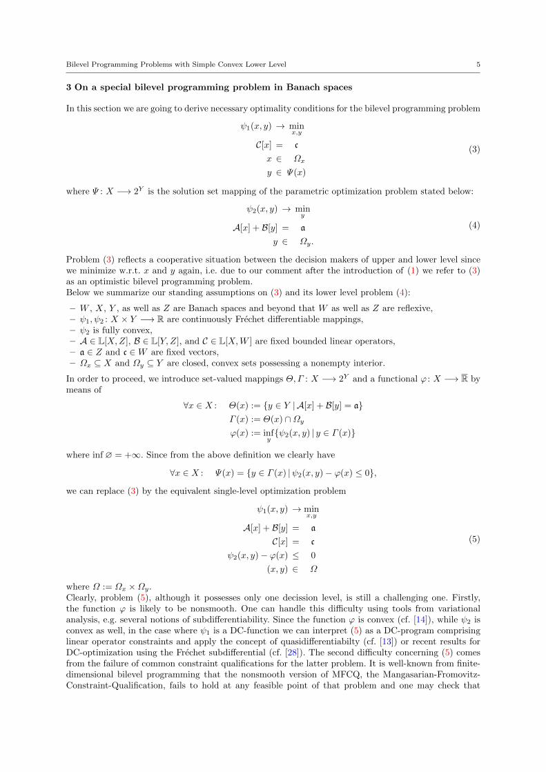
3 On a special bilevel programming problem in Banach spaces
In this section we are going to derive necessary optimality conditions for the bilevel programming problem
ψ1(x, y) → minx,y
C[x] = c
x ∈ Ωx
y ∈ Ψ(x)
(3)
where Ψ : X −→ 2Y is the solution set mapping of the parametric optimization problem stated below:
ψ2(x, y) → miny
A[x] + B[y] = a
y ∈ Ωy.
(4)
Problem (3) reflects a cooperative situation between the decision makers of upper and lower level sincewe minimize w.r.t. x and y again, i.e. due to our comment after the introduction of (1) we refer to (3)as an optimistic bilevel programming problem.Below we summarize our standing assumptions on (3) and its lower level problem (4):
– W , X, Y , as well as Z are Banach spaces and beyond that W as well as Z are reflexive,– ψ1, ψ2 : X × Y −→ R are continuously Frechet differentiable mappings,– ψ2 is fully convex,– A ∈ L[X,Z], B ∈ L[Y, Z], and C ∈ L[X,W ] are fixed bounded linear operators,– a ∈ Z and c ∈W are fixed vectors,– Ωx ⊆ X and Ωy ⊆ Y are closed, convex sets possessing a nonempty interior.
In order to proceed, we introduce set-valued mappings Θ,Γ : X −→ 2Y and a functional ϕ : X −→ R bymeans of
∀x ∈ X : Θ(x) := y ∈ Y | A[x] + B[y] = aΓ (x) := Θ(x) ∩Ωyϕ(x) := inf
yψ2(x, y) | y ∈ Γ (x)
where inf ∅ = +∞. Since from the above definition we clearly have
∀x ∈ X : Ψ(x) = y ∈ Γ (x) |ψ2(x, y)− ϕ(x) ≤ 0,
we can replace (3) by the equivalent single-level optimization problem
ψ1(x, y) → minx,y
A[x] + B[y] = a
C[x] = c
ψ2(x, y)− ϕ(x) ≤ 0
(x, y) ∈ Ω
(5)
where Ω := Ωx ×Ωy.Clearly, problem (5), although it possesses only one decission level, is still a challenging one. Firstly,the function ϕ is likely to be nonsmooth. One can handle this difficulty using tools from variationalanalysis, e.g. several notions of subdifferentiability. Since the function ϕ is convex (cf. [14]), while ψ2 isconvex as well, in the case where ψ1 is a DC-function we can interpret (5) as a DC-program comprisinglinear operator constraints and apply the concept of quasidifferentiabilty (cf. [13]) or recent results forDC-optimization using the Frechet subdifferential (cf. [28]). The second difficulty concerning (5) comesfrom the failure of common constraint qualifications for the latter problem. It is well-known from finite-dimensional bilevel programming that the nonsmooth version of MFCQ, the Mangasarian-Fromovitz-Constraint-Qualification, fails to hold at any feasible point of that problem and one may check that
6 Patrick Mehlitz
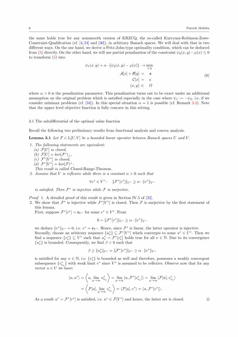
the same holds true for any nonsmooth version of KRZCQ, the so-called Kurcyusz-Robinson-Zowe-Constraint-Qualification (cf. [4, 24] and [30]), in arbitrary Banach spaces. We will deal with that in twodifferent ways. On the one hand, we derive a Fritz-John-type optimality condition, which can be deducedfrom (5) directly. On the other hand, we will use partial penalization of the constraint ψ2(x, y)−ϕ(x) ≤ 0to transform (5) into
ψ1(x, y) + α ·(ψ2(x, y)− ϕ(x)
)→ min
x,y
A[x] + B[y] = a
C[x] = c
(x, y) ∈ Ω
(6)
where α > 0 is the penalization parameter. This penalization turns out to be exact under an additionalassumption on the original problem which is satisfied especially in the case where ψ1 := −ψ2, i.e. if weconsider minimax problems (cf. [34]). In this special situation α = 1 is possible (cf. Remark 3.3). Notethat the upper level objective function is fully concave in this setting.
3.1 The subdifferential of the optimal value function
Recall the following two preliminary results from functional analysis and convex analysis.
Lemma 3.1 Let F ∈ L[U, V ] be a bounded linear operator between Banach spaces U and V .
1. The following statements are equivalent:(a) F [U ] is closed,(b) F [U ] = ker(F∗)⊥,(c) F∗[V ∗] is closed,(d) F∗[V ∗] = ker(F)⊥.This result is called Closed-Range-Theorem.
2. Assume that V is reflexive while there is a constant α > 0 such that
∀v∗ ∈ V ∗ : ‖F∗[v∗]‖U∗ ≥ α · ‖v∗‖V ∗
is satisfied. Then F∗ is injective while F is surjective.
Proof 1. A detailed proof of this result is given in Section IV.5 of [32].2. We show that F∗ is injective while F∗[V ∗] is closed. Then F is surjective by the first statement of
this lemma.First, suppose F∗[v∗] = oU∗ for some v∗ ∈ V ∗. From
0 = ‖F∗[v∗]‖U∗ ≥ α · ‖v∗‖V ∗
we deduce ‖v∗‖V ∗ = 0, i.e. v∗ = oV ∗ . Hence, since F∗ is linear, the latter operator is injective.Secondly, choose an arbitrary sequence u∗ν ⊆ F∗[V ∗] which converges to some u∗ ∈ U∗. Then wefind a sequence v∗ν ⊆ V ∗ such that u∗ν = F∗[v∗ν ] holds true for all ν ∈ N. Due to its convergenceu∗ν is bounded. Consequently, we find β > 0 such that
β ≥ ‖u∗ν‖U∗ = ‖F∗[v∗]‖U∗ ≥ α · ‖v∗‖V ∗
is satisfied for any ν ∈ N, i.e. v∗ν is bounded as well and therefore, possesses a weakly convergentsubsequence v∗νµ with weak limit v∗ since V ∗ is assumed to be reflexive. Observe now that for anyvector u ∈ U we have:
〈u, u∗〉 =
⟨u, limµ→∞
u∗νµ
⟩= limµ→∞
〈u,F∗[v∗νµ ]〉 = limµ→∞
〈F [u], v∗νµ〉
=
⟨F [u], lim
µ→∞v∗νµ
⟩= 〈F [u], v∗〉 = 〈u,F∗[v∗]〉.
As a result u∗ = F∗[v∗] is satisfied, i.e. u∗ ∈ F [V ∗] and hence, the latter set is closed. ut
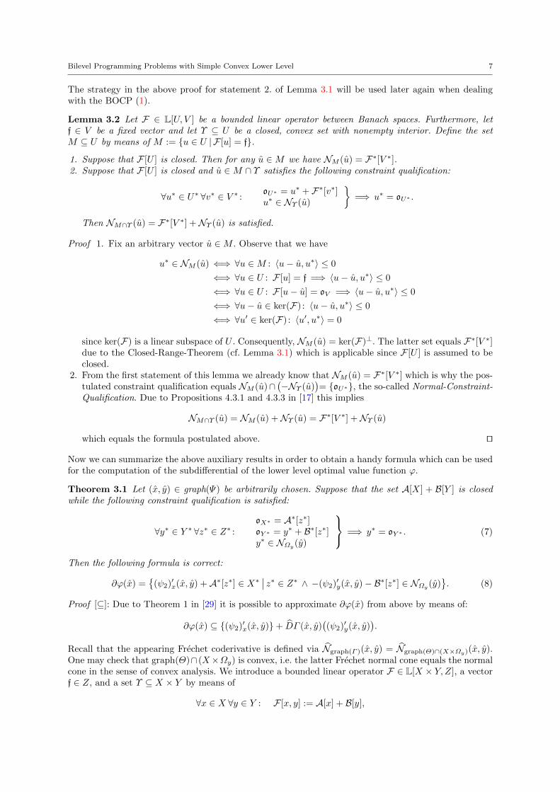
Bilevel Programming Problems with Simple Convex Lower Level 7
The strategy in the above proof for statement 2. of Lemma 3.1 will be used later again when dealingwith the BOCP (1).
Lemma 3.2 Let F ∈ L[U, V ] be a bounded linear operator between Banach spaces. Furthermore, letf ∈ V be a fixed vector and let Υ ⊆ U be a closed, convex set with nonempty interior. Define the setM ⊆ U by means of M := u ∈ U | F [u] = f.
1. Suppose that F [U ] is closed. Then for any u ∈M we have NM (u) = F∗[V ∗].2. Suppose that F [U ] is closed and u ∈M ∩ Υ satisfies the following constraint qualification:
∀u∗ ∈ U∗ ∀v∗ ∈ V ∗ :oU∗ = u∗ + F∗[v∗]u∗ ∈ NΥ (u)
=⇒ u∗ = oU∗ .
Then NM∩Υ (u) = F∗[V ∗] +NΥ (u) is satisfied.
Proof 1. Fix an arbitrary vector u ∈M . Observe that we have
u∗ ∈ NM (u) ⇐⇒ ∀u ∈M : 〈u− u, u∗〉 ≤ 0
⇐⇒ ∀u ∈ U : F [u] = f =⇒ 〈u− u, u∗〉 ≤ 0
⇐⇒ ∀u ∈ U : F [u− u] = oV =⇒ 〈u− u, u∗〉 ≤ 0
⇐⇒ ∀u− u ∈ ker(F) : 〈u− u, u∗〉 ≤ 0
⇐⇒ ∀u′ ∈ ker(F) : 〈u′, u∗〉 = 0
since ker(F) is a linear subspace of U . Consequently, NM (u) = ker(F)⊥. The latter set equals F∗[V ∗]due to the Closed-Range-Theorem (cf. Lemma 3.1) which is applicable since F [U ] is assumed to beclosed.
2. From the first statement of this lemma we already know that NM (u) = F∗[V ∗] which is why the pos-tulated constraint qualification equals NM (u)∩
(−NΥ (u)
)= oU∗, the so-called Normal-Constraint-
Qualification. Due to Propositions 4.3.1 and 4.3.3 in [17] this implies
NM∩Υ (u) = NM (u) +NΥ (u) = F∗[V ∗] +NΥ (u)
which equals the formula postulated above. ut
Now we can summarize the above auxiliary results in order to obtain a handy formula which can be usedfor the computation of the subdifferential of the lower level optimal value function ϕ.
Theorem 3.1 Let (x, y) ∈ graph(Ψ) be arbitrarily chosen. Suppose that the set A[X] + B[Y ] is closedwhile the following constraint qualification is satisfied:
∀y∗ ∈ Y ∗ ∀z∗ ∈ Z∗ :oX∗ = A∗[z∗]oY ∗ = y∗ + B∗[z∗]y∗ ∈ NΩy (y)
=⇒ y∗ = oY ∗ . (7)
Then the following formula is correct:
∂ϕ(x) =
(ψ2)′x(x, y) +A∗[z∗] ∈ X∗∣∣ z∗ ∈ Z∗ ∧ −(ψ2)′y(x, y)− B∗[z∗] ∈ NΩy (y)
. (8)
Proof [⊆]: Due to Theorem 1 in [29] it is possible to approximate ∂ϕ(x) from above by means of:
∂ϕ(x) ⊆ (ψ2)′x(x, y)+ DΓ (x, y)((ψ2)′y(x, y)
).
Recall that the appearing Frechet coderivative is defined via Ngraph(Γ )(x, y) = Ngraph(Θ)∩(X×Ωy)(x, y).One may check that graph(Θ)∩ (X×Ωy) is convex, i.e. the latter Frechet normal cone equals the normalcone in the sense of convex analysis. We introduce a bounded linear operator F ∈ L[X × Y, Z], a vectorf ∈ Z, and a set Υ ⊆ X × Y by means of
∀x ∈ X ∀y ∈ Y : F [x, y] := A[x] + B[y],

8 Patrick Mehlitz
f := a, and Υ := X ×Ωy. Observe that graph(Θ) = (x, y) ∈ X × Y | F [x, y] = f is satisfied while Υ isa closed, convex set possessing a nonempty interior. It is easy to check that the adjoint operator of F isgiven by means of
∀z∗ ∈ Z∗ : F∗[z∗] = (A∗[z∗],B∗[z∗]).
Hence, due to the postulated constraint qualification it is possible to apply statement 2. of Lemma 3.2in order to derive
Ngraph(Θ)∩(X×Ωy)(x, y) = F∗[Z∗] +NΥ (x, y) = F∗[Z∗] + oX∗ × NΩy (y)
=
(A∗[z∗],B∗[z∗] + y∗) ∈ X∗ × Y ∗∣∣ y∗ ∈ NΩy (y) ∧ z∗ ∈ Z∗
.
Finally, we take a closer look on the definition of the Frechet coderivative to obtain
∂ϕ(x) ⊆
(ψ2)′x(x, y) +A∗[z∗] ∈ X∗∣∣ z∗ ∈ Z∗ ∧ −(ψ2)′y(x, y)− B∗[z∗] ∈ NΩy (y)
.
[⊇]: Take an arbitrary element x∗ ∈ X∗ from the set on the right of (8). Then there exist z∗ ∈ Z∗ andy∗ ∈ NΩy (y) satisfying x∗ = (ψ2)′x(x, y) +A∗[z∗] and oY ∗ = (ψ2)′y(x, y) + B∗[z∗] + y∗. Suppose that x∗
is no element of the set ∂ϕ(x). Then there is a vector x ∈ X which satisfies
ϕ(x) < ϕ(x) + 〈x− x, x∗〉.
From ϕ(x) < ϕ(x) + 〈x − x, x∗〉 < +∞ and (x, y) ∈ graph(Ψ) there must exist a vector y ∈ Γ (x) suchthat
ψ2(x, y) < ϕ(x) + 〈x− x, x∗〉 = ψ2(x, y) + 〈x− x, x∗〉
holds. Taking the convexity of ψ2 into consideration it is possible to deduce
ψ2(x, y) < ψ2(x, y) + 〈x− x, x∗〉 = ψ2(x, y) + (ψ2)′x(x, y)[x− x] + 〈x− x,A∗[z∗]〉≤ ψ2(x, y) + (ψ2)′x(x, y)[x− x] + 〈A[x− x], z∗〉+ 〈y − y,−y∗〉= ψ2(x, y) + ψ′2(x, y)[x− x, y − y] + 〈A[x− x] + B[y − y], z∗〉≤ ψ2(x, y) + 〈A[x] + B[x], z∗〉 − 〈A[x] + B[y], z∗〉= ψ2(x, y) + 〈a, z∗〉 − 〈a, z∗〉 = ψ2(x, y),
which clearly is a contradiction. Hence, x∗ ∈ ∂ϕ(x) holds true. ut
Remark 3.1 Assume that Z is a reflexive Banach space while there is a constant α > 0 such that
∀z∗ ∈ Z∗ : ‖A∗[z∗]‖X∗ ≥ α · ‖z∗‖Z∗
is satisfied. Then the assumptions of Theorem 3.1 hold at any point (x, y) ∈ graph(Ψ).
Proof From statement 2. of Lemma 3.1 we know that A∗ is injective while A is surjective. Hence,Z = A[X] ⊆ A[X] + B[Y ] ⊆ Z leads to A[X] + B[Y ] = Z, i.e. A[X] + B[Y ] is closed. Now choosean arbitrary point (x, y) ∈ graph(Ψ) as well as y∗ ∈ Y ∗ and z∗ ∈ Z∗ which satisfy oX∗ = A∗[z∗],oY ∗ = y∗+B∗[z∗], and y∗ ∈ NΩy (y). Since A∗ is injective, the condition oX∗ = A∗[z∗] implies z∗ = oZ∗ .Taking oY ∗ = y∗ + B∗[z∗] into account we have y∗ = oY ∗ . That is why the constraint qualification (7)holds as well. ut
3.2 Necessary optimality conditions
We start with a Fritz-John-type necessary optimality condition for the bilevel programming problem (3)with fully convex functional ψ1 which can be verified very easily.
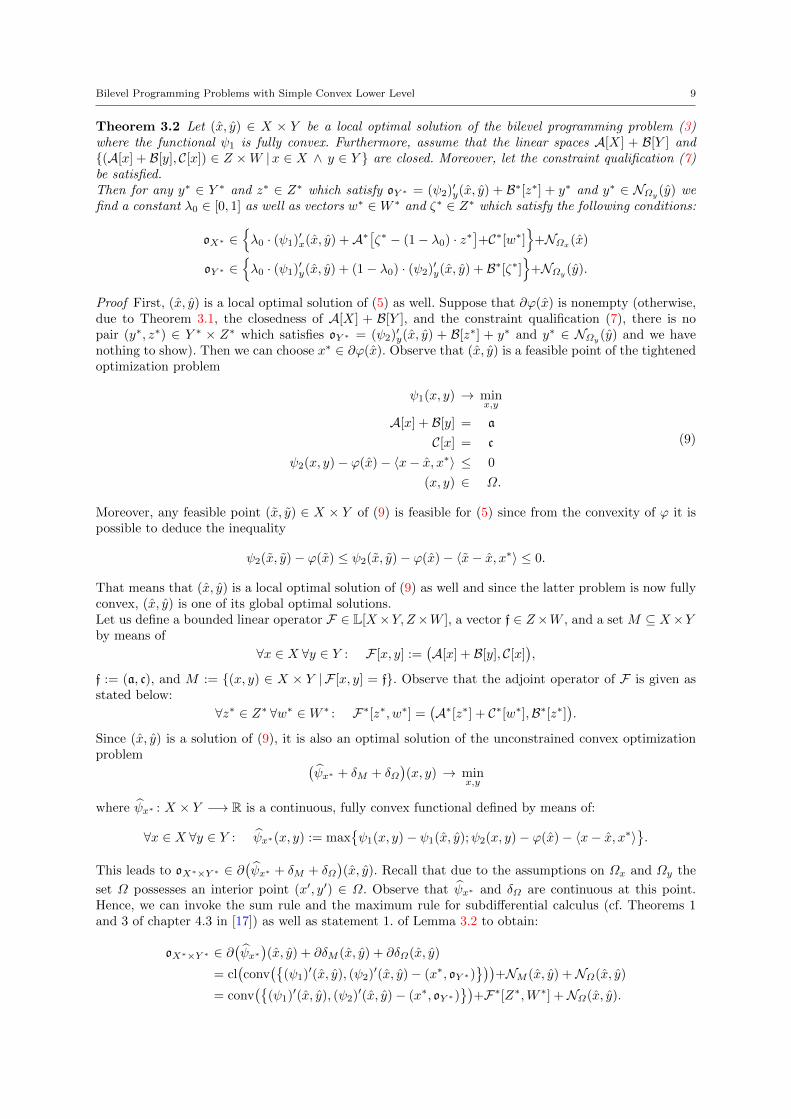
Bilevel Programming Problems with Simple Convex Lower Level 9
Theorem 3.2 Let (x, y) ∈ X × Y be a local optimal solution of the bilevel programming problem (3)where the functional ψ1 is fully convex. Furthermore, assume that the linear spaces A[X] + B[Y ] and(A[x] + B[y], C[x]) ∈ Z ×W |x ∈ X ∧ y ∈ Y are closed. Moreover, let the constraint qualification (7)be satisfied.Then for any y∗ ∈ Y ∗ and z∗ ∈ Z∗ which satisfy oY ∗ = (ψ2)′y(x, y) + B∗[z∗] + y∗ and y∗ ∈ NΩy (y) wefind a constant λ0 ∈ [0, 1] as well as vectors w∗ ∈W ∗ and ζ∗ ∈ Z∗ which satisfy the following conditions:
oX∗ ∈λ0 · (ψ1)′x(x, y) +A∗
[ζ∗ − (1− λ0) · z∗
]+C∗[w∗]
+NΩx(x)
oY ∗ ∈λ0 · (ψ1)′y(x, y) + (1− λ0) · (ψ2)′y(x, y) + B∗[ζ∗]
+NΩy (y).
Proof First, (x, y) is a local optimal solution of (5) as well. Suppose that ∂ϕ(x) is nonempty (otherwise,due to Theorem 3.1, the closedness of A[X] + B[Y ], and the constraint qualification (7), there is nopair (y∗, z∗) ∈ Y ∗ × Z∗ which satisfies oY ∗ = (ψ2)′y(x, y) + B[z∗] + y∗ and y∗ ∈ NΩy (y) and we havenothing to show). Then we can choose x∗ ∈ ∂ϕ(x). Observe that (x, y) is a feasible point of the tightenedoptimization problem
ψ1(x, y) → minx,y
A[x] + B[y] = a
C[x] = c
ψ2(x, y)− ϕ(x)− 〈x− x, x∗〉 ≤ 0
(x, y) ∈ Ω.
(9)
Moreover, any feasible point (x, y) ∈ X × Y of (9) is feasible for (5) since from the convexity of ϕ it ispossible to deduce the inequality
ψ2(x, y)− ϕ(x) ≤ ψ2(x, y)− ϕ(x)− 〈x− x, x∗〉 ≤ 0.
That means that (x, y) is a local optimal solution of (9) as well and since the latter problem is now fullyconvex, (x, y) is one of its global optimal solutions.Let us define a bounded linear operator F ∈ L[X×Y,Z×W ], a vector f ∈ Z×W , and a set M ⊆ X×Yby means of
∀x ∈ X ∀y ∈ Y : F [x, y] :=(A[x] + B[y], C[x]
),
f := (a, c), and M := (x, y) ∈ X × Y | F [x, y] = f. Observe that the adjoint operator of F is given asstated below:
∀z∗ ∈ Z∗ ∀w∗ ∈W ∗ : F∗[z∗, w∗] =(A∗[z∗] + C∗[w∗],B∗[z∗]
).
Since (x, y) is a solution of (9), it is also an optimal solution of the unconstrained convex optimizationproblem (
ψx∗ + δM + δΩ)(x, y) → min
x,y
where ψx∗ : X × Y −→ R is a continuous, fully convex functional defined by means of:
∀x ∈ X ∀y ∈ Y : ψx∗(x, y) := maxψ1(x, y)− ψ1(x, y);ψ2(x, y)− ϕ(x)− 〈x− x, x∗〉
.
This leads to oX∗×Y ∗ ∈ ∂(ψx∗ + δM + δΩ
)(x, y). Recall that due to the assumptions on Ωx and Ωy the
set Ω possesses an interior point (x′, y′) ∈ Ω. Observe that ψx∗ and δΩ are continuous at this point.Hence, we can invoke the sum rule and the maximum rule for subdifferential calculus (cf. Theorems 1and 3 of chapter 4.3 in [17]) as well as statement 1. of Lemma 3.2 to obtain:
oX∗×Y ∗ ∈ ∂(ψx∗)(x, y) + ∂δM (x, y) + ∂δΩ(x, y)
= cl(conv
((ψ1)′(x, y), (ψ2)′(x, y)− (x∗, oY ∗)
))+NM (x, y) +NΩ(x, y)
= conv(
(ψ1)′(x, y), (ψ2)′(x, y)− (x∗, oY ∗))
+F∗[Z∗,W ∗] +NΩ(x, y).
10 Patrick Mehlitz
Hence, due to the representation of F∗ presented above, there exist λ0 ∈ [0, 1] and vectors w∗ ∈ W ∗ aswell as ζ∗ ∈ Z∗ such that
oX∗ ∈λ0 · (ψ1)′x(x, y) + (1− λ0) ·
((ψ2)′x(x, y)− x∗
)+A∗[ζ∗] + C∗[w∗]
+NΩx(x)
oY ∗ ∈λ0 · (ψ1)′y(x, y) + (1− λ0) · (ψ2)′y(x, y) + B∗[ζ∗]
+NΩy (y)
is satisfied. Finally, we make use of Theorem 3.1 in order to see that x∗ ∈ ∂ϕ(x) holds true if and only ifthere exist y∗ ∈ Y ∗ and z∗ ∈ Z∗, such that the conditions oY ∗ = (ψ2)′y(x, y) +B∗[z∗] + y∗, y∗ ∈ NΩy (y),and x∗ = (ψ2)′x(x, y) +A∗[z∗] hold. We plug this representation of the subgradient x∗ into the inclusionon the x-component stated above to obtain the necessary optimality condition of the theorem. ut
Remark 3.2 Let B and C be surjective bounded linear operators. Then the linear spaces A[X] + B[Y ]and (A[x] + B[y], C[x]) ∈ Z ×W |x ∈ X ∧ y ∈ Y are closed.
One of the major disadvantages of the necessary optimality condition presented in Theorem 3.2 turnsout to be the appearence of the multiplier λ0, which is allowed to be zero. The latter case leads to theextinction of ψ1 from the necessary optimality conditions and choosing w∗ := oW∗ and ζ∗ := z∗ onealways can satisfy the conditions in Theorem 3.2. Hence, we want to avoid this situation. Therefore, weneed an additional property of problem (3).
Definition 3.1 Let (x, y) ∈ X × Y be a local optimal solution of the bilevel programming problem (3).The latter problem is called partially calm at (x, y) provided there exist α > 0 and ε > 0 such that forany feasible point (x, y) ∈ UεX×Y (x, y) of (6) the following inequality holds:
ψ1(x, y)− ψ1(x, y) + α ·(ψ2(x, y)− ϕ(x)
)≥ 0.
Partial calmness was first introduced by Ye and Zhu in [34] where the authors derived necessary optimalityconditions for finite-dimensional bilevel programming problems. In [12] and [34] some classes of finite-dimensional bilevel programming problems are presented which possess the property to be partially calmat any local optimal solution. The concept of partial calmness was generalized to infinite-dimensionalbilevel programming in [2, 3] and [33] where the authors deal with bilevel optimal control problems.An important observation is recorded in the next lemma. Its proof is omited here since it is just ageneralization of the proofs of similar results stated in [2, 3] and [34].
Lemma 3.3 Let (x, y) ∈ X × Y be a local optimal solution of the bilevel programming problem (3). Thelatter problem is partially calm at (x, y) if and only if there exists a constant α > 0 such that (x, y) is alocal optimal solution of (6).
For minimax problems we obtain the following obvious but important fact.
Remark 3.3 Let (x, y) ∈ X ×Y be a local optimal solution of the bilevel programming problem (3) withψ1 := −ψ2. Then (x, y) is a local optimal solution for (6) with α := 1 as well.
Due to Lemma 3.3 and Remark 3.3 it is clear that any minimax problem is partially calm at its localoptimal solutions.Now it is possible to state a necessary optimality condition of KKT-type.
Theorem 3.3 Let (x, y) ∈ X × Y be a local optimal solution of the bilevel programming problem (3)where ψ1 is fully convex or fully concave. Suppose that the assumptions of Theorem 3.2 hold while (3) ispartially calm at (x, y).Then there exists a constant α > 0 such that for any vectors y∗ ∈ Y ∗ and z∗ ∈ Z∗ which satisfyoY ∗ = (ψ2)′y(x, y) + B∗[z∗] + y∗ and y∗ ∈ NΩy (y) we find vectors w∗ ∈ W ∗ and ζ∗ ∈ Z∗ which satisfythe following conditions:
oX∗ ∈
(ψ1)′x(x, y) +A∗[ζ∗ − α · z∗
]+C∗[w∗]
+NΩx(x)
oY ∗ ∈
(ψ1)′y(x, y) + α · (ψ2)′y(x, y) + B∗[ζ∗]
+NΩy (y).
Bilevel Programming Problems with Simple Convex Lower Level 11
Proof We start with the proof for the case where ψ1 is convex and just mention below what we have tochange in order to obtain the same result for concave functionals ψ1.Let ψ1 be fully convex. Since (3) is partially calm at (x, y), due to Lemma 3.3 there exists α > 0such that the latter point is a local optimal solution of (6). We introduce the bounded linear operatorF ∈ L[X × Y,Z ×W ], the vector f ∈ Z ×W , and the set M ⊆ X × Y as it was done in the proof ofTheorem 3.2. Hence, (x, y) is a local optimal solution of the unconstrained optimization problem(
ψ1 + α · ψ2 + δM + δΩ)(x, y)− α · ϕ(x) → min
x,y. (10)
Observe that ψ1 + α · ψ2 + δM + δΩ and α · ϕ are convex functions, i.e. (10) is a DC-program. Hence,Proposition 4.1 in [28] is applicable and we obtain:
α · ∂ϕ(x)×oY ∗
⊆ ∂
(ψ1 + α · ψ2 + δM + δΩ
)(x, y). (11)
A similar argumentation as in the proof of Theorem 3.2 yields:
α · ∂ϕ(x)×oY ∗
⊆
(ψ1)′(x, y) + α · (ψ2)′(x, y)
+F∗[Z∗,W ∗] +NΩ(x, y). (12)
Due to Theorem 3.1 the set ∂ϕ(x) is empty if and only if there is no pair (y∗, z∗) ∈ Y ∗ × Z∗ whichsatisfies oY ∗ = (ψ2)′y(x, y) + B∗[z∗] + y∗ and y∗ ∈ NΩy (y) but in the latter case the statement of thistheorem holds trivially. Hence, take an arbitrary subgradient x∗ ∈ ∂ϕ(x) and observe that from (12) itis possible to derive the existence of w∗ ∈W ∗ and ζ∗ ∈ Z∗ satisfying
oX∗ ∈
(ψ1)′x(x, y) + α ·((ψ2)′x(x, y)− x∗
)+A∗[ζ∗] + C∗[w∗]
+NΩx(x)
oY ∗ ∈
(ψ1)′y(x, y) + α · (ψ2)′y(x, y) + B∗[ζ∗]
+NΩy (y).
Since by Theorem 3.1 x∗ ∈ ∂ϕ(x) holds true if and only if there exists a pair (y∗, z∗) ∈ Y ∗×Z∗ such thatoY ∗ = (ψ2)′y(x, y)+B∗[z∗]+y∗, y∗ ∈ NΩy (y), and x∗ = (ψ2)′x(x, y)+A∗[z∗] are satisfied, we easily derivethe statement of the theorem by plugging this representation of x∗ into the inclusion on the x-componentstated earlier. This completes the proof for the case where ψ1 is fully convex.Assume that ψ1 is fully concave. A similar argumentation as presented above shows that (x, y) is a localoptimal solution of the unconstrained optimization problem(
α · ψ2 + δM + δΩ)(x, y)−
(α · ϕ− ψ1
)(x) → min
x,y(13)
for some α > 0. Obviously, (13) is a DC-program as well and Proposition 4.1 in [28] yields the necessaryoptimality condition
∂(α · ϕ− ψ1
)(x, y) ⊆ ∂
(α · ψ2 + δM + δΩ
)(x, y). (14)
Using the calculus rules for subdifferentials once more, while noting that −ψ1 is continuously Frechetdifferentiable and convex leads to (12) again. The remaining part of the proof is the same as in theconvex case.This completes the proof of the whole theorem. ut
Remark 3.4 Note that the conditions (11) and (14) can also be obtained using the theory of quasidiffer-entiability which is presented in [13].
A typical setting where all the assumptions of Theorem 3.3 are satisfied is presented below.
Example 3.1 Let X = Rn, Y = Rm, W = Rr, Z = Rs, Ωx = Rn,+0 , and Ωy = Rm,+0 be satisfied.Furthermore, assume that A ∈ Rs×n, B ∈ Rs×m, C ∈ Rr×n, a ∈ Rs, c ∈ Rr, and d ∈ Rm are fixedmatrices, let ψ1 be fully convex or fully concave, and let (3) be given as stated below:
ψ1(x, y) → minx,y
Cx = c
x ≥ 0n
y ∈ Ψ(x) := Argminy
d>y |Ax+By = a, y ≥ 0m
.
(15)
12 Patrick Mehlitz
Due to [34] this problem is partially calm at any of its local optimal solutions. Due to the finite-dimensional setting the closedness conditions on the subspaces mentioned in the assumptions of Theorem3.3 hold trivially. We can state a slightly stronger version of the constraint qualification (7) which is in-dependent of the considered point by means of:
@z∗ ∈ Rs : A>z∗ = 0n ∧ B>z∗ ≥ 0m ∧ B>z∗ 6= 0m.
Applying Motzkin’s alternative theorem this is equivalent to:
∃µ ∈ Rn ∃λ ∈ Rm,+ : Aµ+Bλ = 0s. (16)
We only needed the constraint qualification (7) within the proof of Theorem 3.3 in order to guaranteeequation (8). It is well-known from finite-dimensional linear programming and the corresponding dualitytheory that the formula
∂ϕ(x) =A>z∗ ∈ Rn | ∃z∗ ∈ Rs : 0m ≤ d+B>z∗ ∧ 0 = y>
(d+B>z∗
),
which equals (8) in this setting, holds true for any point y ∈ Ψ(x) without any further assumption, i.e.we do not need (16) or even (7) to be satisfied in order to apply the necessary optimality conditions fromTheorem 3.3.Hence, if (x, y) ∈ Rn × Rm is a local optimal solution of (15), then there is α > 0 such that, wheneverz∗ ∈ Rs satisfies 0m ≤ d+B>z∗ and 0 = y>(d+B>z∗), there exist w∗ ∈ Rr and ζ∗ ∈ Rs which satisfythe following conditions:
0n ≤ ∇xψ1(x, y)> +A>(ζ∗ − α · z∗
)+C>w∗
0m ≤ ∇yψ1(x, y)> + α · d+B>ζ∗
0 = x>(∇xψ1(x, y)> +A>
(ζ∗ − α · z∗
)+C>w∗
)0 = y>
(∇yψ1(x, y)> + α · d+B>ζ∗
).
Note that if ψ1 is chosen as a linear functional, then (15) coincides with the so-called linear bilevelprogramming problem and necessary optimality conditions for the latter program are given in manypublications e.g. in [8] and [34]. utTheorem 3.3 can be specified in terms of minimax problems.
Corollary 3.1 Let (x, y) ∈ X×Y be a local optimal solution of (3) where ψ1 := −ψ2 is satisfied. Supposethat the assumptions of Theorem 3.2 hold. Then the following statements are correct.
1. For any y∗ ∈ Y ∗ and z∗ ∈ Z∗ which satisfy oY ∗ = (ψ2)′y(x, y) +B∗[z∗] + y∗ and y∗ ∈ NΩy (y) we findvectors w∗ ∈W ∗ and ζ∗ ∈ Z∗ such that the following conditions hold:
oX∗ ∈−(ψ2)′x(x, y) +A∗
[ζ∗ − z∗
]+C∗[w∗]
+NΩx(x)
oY ∗ ∈B∗[ζ∗]
+NΩy (y).
2. Suppose that B[cone(Ωy − y)] = Z holds true. Then for any y∗ ∈ Y ∗ and z∗ ∈ Z∗ which satisfyoY ∗ = (ψ2)′y(x, y) + B∗[z∗] + y∗ and y∗ ∈ NΩy (y) we find a vector w∗ ∈ W ∗ such that the followingcondition holds:
oX∗ ∈−(ψ2)′x(x, y)−A∗
[z∗]+C∗[w∗]
+NΩx(x).
Proof 1. Due to Remark 3.3 the corresponding problem (3) is partially calm at (x, y) and the latter pointis an optimal solution for problem (6) with α = 1. From ψ1 = −ψ2 we know that ψ1 is fully concave.Consequently, Theorem 3.3 is applicable and yields the above necessary optimality conditions.
2. We dualize B[cone(Ωy − y)] = Z in order to obtain:
ζ∗ ∈ Z∗ | ∀y ∈ Ωy : 〈y − y,B∗[ζ∗]〉 ≥ 0 = oZ∗ .
This yields that whenever B∗[ζ∗] belongs to −NΩy (y) for some ζ∗ ∈ Z∗ then ζ∗ = oZ∗ is satisfied.Hence, this statement just follows from the first one noting that ζ∗ vanishes. ut
Remark 3.5 For any point (x, y) ∈ graph(Γ ) the condition B∗[cone(Ωy − y)] = Z appearing in thesecond statement of Corollary 3.1 equals KRZCQ at (x, y) w.r.t. to the decision variable y for the lowerlevel problem (4) (cf. [4]). Obviously, this condition is stronger than (7).
Bilevel Programming Problems with Simple Convex Lower Level 13
4 Optimality conditions for the bilevel optimal control problem
4.1 Formalisation of the problem
We start by introducing certain Banach spaces, functionals, linear operators, and sets which allow us tointerpret (1) as a problem of type (3).First, we set:
W := Wn1,p(0, T )× Rr
X := Wn1,p(0, T )× Lkp(0, T )
Y := Wm1,p(0, T )× Llp(0, T )
Z := Wm1,p(0, T )× Rs.
Next, we define Frechet differentiable convex functionals ψ1, ψ2 : X × Y −→ R by means of
ψ1(x, u, y, v) := f(x(0), x(T ), y(0), y(T )) +
∫ T
0
F (t, x(t), y(t), u(t), v(t))dt
ψ2(x, u, y, v) := g(x(0), x(T ), y(0), y(T )) +
∫ T
0
G(t, x(t), y(t), u(t), v(t))dt
for any (x, u) ∈ X and (y, v) ∈ Y . Furthermore, we make use of the bounded linear operatorsA ∈ L[X,Z],B ∈ L[Y,Z], and C ∈ L[X,W ] given below for any (x, u) ∈ X and (y, v) ∈ Y :
A[x, u] :=
(−∫ ·0
[Axx(τ) +Auu(τ)
]dτ, A0x(0)
)B[y, v] :=
(y(·)− y(0)−
∫ ·0
[Byy(τ) +Bvv(τ)
]dτ, B0y(0)
)C[x, u] :=
(x(·)− x(0)−
∫ ·0
[Cxx(τ) + Cuu(τ)
]dτ, C0x(0) + CTx(T )
).
We introduce a := (oWm1,p(0,T ), a), c := (oWn
1,p(0,T ), c), Ωx := Wn1,p(0, T )×U , and Ωy := Wm
1,p(0, T )×V in
order to see that (1) is a problem of type (3).For a fixed point (x, u, y, v) ∈ X×Y and t ∈ (0, T ) we want to use the following space-saving abbreviationsin the upcoming proofs:
f(0, T ) := f(x(0), x(T ), y(0), y(T ))
F (t) := F (t, x(t), y(t), u(t), v(t))
g(0, T ) := g(x(0), x(T ), y(0), y(T ))
G(t) := G(t, x(t), y(t), u(t), v(t)).
The next lemma reveals how the Frechet derivatives of ψ1 and ψ2 as well as the adjoint operators of A,B, and C look like.
14 Patrick Mehlitz
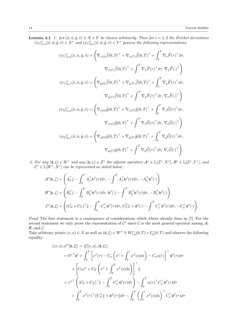
Lemma 4.1 1. Let (x, u, y, v) ∈ X × Y be chosen arbitrarily. Then for i = 1, 2 the Frechet derivatives(ψi)
′x,u(x, u, y, v) ∈ X∗ and (ψi)
′y,v(x, u, y, v) ∈ Y ∗ possess the following representations:
(ψ1)′x,u(x, u, y, v) =
(∇x(0)f(0, T )> +∇x(T )f(0, T )> +
∫ T
0
∇xF (τ)>dτ,
∇x(T )f(0, T )> +
∫ T
·∇xF (τ)>dτ, ∇uF (·)>
)
(ψ1)′y,v(x, u, y, v) =
(∇y(0)f(0, T )> +∇y(T )f(0, T )> +
∫ T
0
∇yF (τ)>dτ,
∇y(T )f(0, T )> +
∫ T
·∇yF (τ)>dτ, ∇vF (·)>
)
(ψ2)′x,u(x, u, y, v) =
(∇x(0)g(0, T )> +∇x(T )g(0, T )> +
∫ T
0
∇xG(τ)>dτ,
∇x(T )g(0, T )> +
∫ T
·∇xG(τ)>dτ, ∇uG(·)>
)
(ψ2)′y,v(x, u, y, v) =
(∇y(0)g(0, T )> +∇y(T )g(0, T )> +
∫ T
0
∇yG(τ)>dτ,
∇y(T )g(0, T )> +
∫ T
·∇yG(τ)>dτ, ∇vG(·)>
).
2. For any (d, ξ) ∈ W ∗ and any (h, ζ) ∈ Z∗ the adjoint operators A∗ ∈ L[Z∗, X∗], B∗ ∈ L[Z∗, Y ∗], andC∗ ∈ L[W ∗, X∗] can be represented as stated below:
A∗[h, ζ] =
(A>0 ζ −
∫ T
0
A>x hf (τ)dτ, −
∫ T
·A>x h
f (τ)dτ, −A>u hf (·)
)
B∗[h, ζ] =
(B>0 ζ −
∫ T
0
B>y hf (τ)dτ, hf (·)−
∫ T
·B>y h
f (τ)dτ, −B>v hf (·)
)
C∗[d, ξ] =
((C0 + CT )>ξ −
∫ T
0
C>x df (τ)dτ, C>T ξ + df (·)−
∫ T
·C>x d
f (τ)dτ, −C>u df (·)
).
Proof The first statement is a consequence of considerations which where already done in [7]. For thesecond statement we only prove the representation of C∗ since C is the most general operator among A,B, and C.Take arbitrary points (x, u) ∈ X as well as (d, ξ) ∈W ∗ ∼= Wn
1,q(0, T )×Lrq(0, T ) and observe the followingequality:
〈(x, u), C∗[d, ξ]〉 = 〈C[x, u], (d, ξ)〉
= 0n>ds +
∫ T
0
[xf (τ)− Cx
(xs +
∫ τ
0
xf (s)ds
)− Cuu(τ)
]>df (τ)dτ
+
[C0x
s + CT
(xs +
∫ T
0
xf (s)ds
)]>ξ
= xs>(
(C0 + CT )>ξ −∫ T
0
C>x df (τ)dτ
)−∫ T
0
u(τ)>C>u df (τ)dτ
+
∫ T
0
xf (τ)>(C>T ξ + df (τ)
)dτ −
∫ T
0
(∫ τ
0
xf (s)ds
)>C>x d
f (τ)dτ

Bilevel Programming Problems with Simple Convex Lower Level 15
= xs>(
(C0 + CT )>ξ −∫ T
0
C>x df (τ)dτ
)−∫ T
0
u(τ)>C>u df (τ)dτ +
∫ T
0
xf (τ)>(C>T ξ + df (τ)
)dτ
−(∫ τ
0
xf (s)ds
)>(∫ τ
0
C>x df (s)ds
) ∣∣∣∣∣T
0
+
∫ T
0
xf (τ)>(∫ τ
0
C>x df (s)ds
)dτ
= xs>(
(C0 + CT )>ξ −∫ T
0
C>x df (τ)dτ
)+
∫ T
0
xf (τ)>
(C>T ξ + df (τ)−
∫ T
τ
C>x df (s)ds
)dτ
−∫ T
0
u(τ)>C>u df (τ)dτ
Now one only has to apply the definition of the dual pairing ofX to come up with the above representationof the operator C∗. ut
4.2 The satisfaction of constraint qualifications
In this section we check stepwise that the constraint qualifications we need in order to apply the resultsfrom Section 3.2 are satisfied for problem (1).
Lemma 4.2 For (1) the linear space A[X] + B[Y ] is closed.
Proof Let us define a bounded linear operator F ∈ L[X × Y,Z] by means of
∀x ∈ X ∀y ∈ Y : F [x, y] := A[x] + B[y].
Then by Lemma 3.1 A[X] + B[Y ] = F [X × Y ] is closed if and only if F∗[Z∗] is closed and it is notdifficult to see that
∀z∗ ∈ Z∗ : F∗[z∗] =(A∗[z∗],B∗[z∗]
)holds true.That is why we take an arbitrary sequence (xν , uν , yν , vν) ⊆ F∗[Z∗] which converges to a point(x, u, y, v) ∈ X∗ × Y ∗. By definition of F and Lemma 4.1 we find a sequence (hν , ζν) ⊆ Z∗ such thatfor any ν ∈ N the following holds true:
xsν = A>0 ζν −∫ T
0
A>x hfν (τ)dτ ysν = B>0 ζν −
∫ T
0
B>y hfν (τ)dτ
xfν (·) = −∫ T
·A>x h
fν (τ)dτ yfν (·) = hfν (·)−
∫ T
·B>y h
fν (τ)dτ
uν(·) = −A>u hfν (·) vν(·) = −B>v hfν (·).
Due to the full row rank assumption on Bv there exists σ1 > 0 such that
‖y‖q =∥∥(BvB
>v )−1BvB
>v y∥∥q≤ σ1 · ‖B>v y‖q
is satisfied for all y ∈ Rm. Due to its convergence vν is bounded. That is why we find a constant M > 0such that for any ν ∈ N the following estimation is correct:
M ≥ ‖vν‖qLlq(0,T )= ‖B>v hfν (·)‖q
Llq(0,T )=
∫ T
0
‖B>v hfν (τ)‖qqdτ ≥1
σq1
∫ T
0
‖hfν (τ)‖qqdτ =1
σq1‖hfν‖
qLmq (0,T ).
Hence, the sequence hfν is a bounded sequence in a reflexive Banach space which is why it possesses aweakly convergent subsequence hfνµ with weak limit hf .
For an arbitrary function v ∈ Llp(0, T ) we now have:
〈v, v〉 = limµ→∞
〈v, vνµ〉 = limµ→∞
〈v,−B>v hfνµ(·)〉 = limµ→∞
〈−Bvv(·), hfνµ〉 = 〈−Bvv(·), hf 〉 = 〈v,−B>v hf (·)〉.
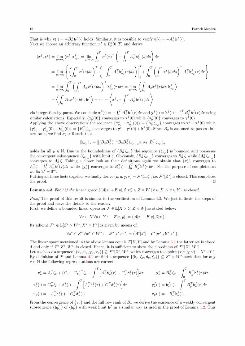
16 Patrick Mehlitz
That is why v(·) = −B>v hf (·) holds. Similarly, it is possible to verify u(·) = −A>u hf (·).Next we choose an arbitrary function xf ∈ Lnp (0, T ) and derive
〈xf , xf 〉 = limµ→∞
〈xf , xfνµ〉 = limµ→∞
∫ T
0
xf (τ)>
(−∫ T
τ
A>x hfνµ(s)ds
)dτ
= limµ→∞
(∫ τ
0
xf (s)ds
)>(−∫ T
τ
A>x hfνµ(s)ds
)∣∣∣∣∣T
0
+
∫ T
0
(∫ τ
0
xf (s)ds
)>A>x h
fνµ(τ)dτ
= limµ→∞
∫ T
0
(∫ τ
0
Axxf (s)ds
)>hfνµ(τ)dτ = lim
µ→∞
⟨∫ ·0
Axxf (τ)dτ, hfνµ
⟩=
⟨∫ ·0
Axxf (τ)dτ, hf
⟩= · · · =
⟨xf ,−
∫ T
·A>x h
f (τ)dτ
⟩
via integration by parts. We conclude xf (·) = −∫ T· A
>x h
f (τ)dτ and yf (·) = hf (·)−∫ T· B
>y h
f (τ)dτ using
similar calculations. Especially, xfν (0) converges to xf (0) while yfν (0) converges to yf (0).Applying the above observations the sequence xsνµ − xfνµ(0) = A>0 ζνµ converges to xs − xf (0) while
ysνµ − yfνµ(0) + hfνµ(0) = B>0 ζνµ converges to ys − yf (0) + hf (0). Since B0 is assumed to possess fullrow rank, we find σ2 > 0 such that
‖ζνµ‖2 =∥∥(B0B
>0 )−1B0B
>0 ζνµ
∥∥2≤ σ2
∥∥B>0 ζνµ∥∥2holds for all µ ∈ N. Due to the boundedness of B>0 ζνµ the sequence ζνµ is bounded and possessesthe convergent subsequence ζνµκ with limit ζ. Obviously, B>0 ζνµκ converges to B>0 ζ while A>0 ζνµκconverges to A>0 ζ. Taking a closer look at their definitions again we obtain that xsν converges to
A>0 ζ −∫ T0A>x h
f (τ)dτ while ysν converges to B>0 ζ −∫ T0B>y h
f (τ)dτ . For the purpose of completenesswe fix hs = 0m.Putting all these facts together we finally derive (x, u, y, v) = F∗[h, ζ], i.e. F∗[Z∗] is closed. This completesthe proof. ut
Lemma 4.3 For (1) the linear space (A[x] + B[y], C[x]) ∈ Z ×W |x ∈ X ∧ y ∈ Y is closed.
Proof The proof of this result is similar to the verification of Lemma 4.2. We just indicate the steps ofthe proof and leave the details to the reader.First, we define a bounded linear operator F ∈ L[X × Y, Z ×W ] as stated below:
∀x ∈ X ∀y ∈ Y : F [x, y] :=(A[x] + B[y], C[x]
).
Its adjoint F∗ ∈ L[Z∗ ×W ∗, X∗ × Y ∗] is given by means of:
∀z∗ ∈ Z∗ ∀w∗ ∈W ∗ : F∗[z∗, w∗] =(A∗[z∗] + C∗[w∗],B∗[z∗]
).
The linear space mentioned in the above lemma equals F [X,Y ] and by Lemma 3.1 the latter set is closedif and only if F∗[Z∗,W ∗] is closed. Hence, it is sufficient to show the closedness of F∗[Z∗,W ∗].Let us choose a sequence (xν , uν , yν , vν) ⊆ F∗[Z∗,W ∗] which converges to a point (x, u, y, v) ∈ X∗×Y ∗.By definition of F and Lemma 4.1 we find a sequence (hν , ζν , dν , ξν) ⊆ Z∗ ×W ∗ such that for anyν ∈ N the following representations are correct:
xsν = A>0 ζν + (C0 + CT )>ξν −∫ T
0
[A>x h
fν (τ) + C>x d
fν (τ)
]dτ ysν = B>0 ζν −
∫ T
0
B>y hfν (τ)dτ
xfν (·) = C>T ξν + dfν (·)−∫ T
·
[A>x h
fν (τ) + C>x d
fν (τ)
]dτ yfν (·) = hfν (·)−
∫ T
·B>y h
fν (τ)dτ
uν(·) = −A>u hfν (·)− C>u dfν (·) vν(·) = −B>v hfν (·).
From the convergence of vν and the full row rank of Bv we derive the existence of a weakly convergentsubsequence hfνµ of hfν with weak limit hf in a similar way as used in the proof of Lemma 4.2. This
Bilevel Programming Problems with Simple Convex Lower Level 17
leads to v(·) = −B>v hfν (·) and yf (·) = hf (·)−∫ T· B
>y h
f (τ)dτ . Furthermore, we make use of the full rowrank of B0 in order to show that ζνµ contains a convergent subsequence ζνµκ whose limit ζ satisfies
ys = B>0 ζ −∫ T0B>y h
f (τ)dτ .
Since hfνµκ converges weakly to hf , the sequence −A>u hfνµκ (·) converges weakly to −A>u hf (·). Observe
that −C>u dfνµκ (·) = uνµκ (·) +A>u hfνµκ
(·) holds true and the latter sequence is at least weakly conver-gent and especially bounded. That is why we can exploit the full row rank assumption on Cu in order toshow that dfνµκ contains a weakly convergent subsequence dfνµκπ with weak limit df . Especially, we
obtain u(·) = −A>u hf (·) − C>u df (·). Furthermore, the weak convergence of dfνµκπ and hfνµκπ as well
as the convergence of ζνµκπ imply the convergence of A>0 ζνµκπ −∫ T0
[A>x hfνµκπ
(τ)+C>x dfνµκπ
(τ)]dτ to
A>0 ζ −∫ T0
[A>x hf (τ) + C>x d
f (τ)]dτ . Recalling that the sequence xsν is convergent as well the sequence
(C0+CT )>ξνµκπ is converent and especially bounded. Due to the full row rank assumption on C0+CTthis leads to the existence of a convergent subsequence of ξνµκπ with limit ξ. Consequently, we obtain
xs = A>0 ζ+(C0+CT )>ξ−∫ T0
[A>x hf (τ)+C>x d
f (τ)]dτ and xf (·) = C>T ξ+df (·)−∫ T· [A>x h
f (τ)+C>x df (τ)]dτ .
Finally, we choose hs = 0m and ds = 0n to see F∗[h, ζ, d, ξ] = (x, u, y, v), i.e. the set F∗[Z∗,W ∗] is closed.This completes the proof. ut
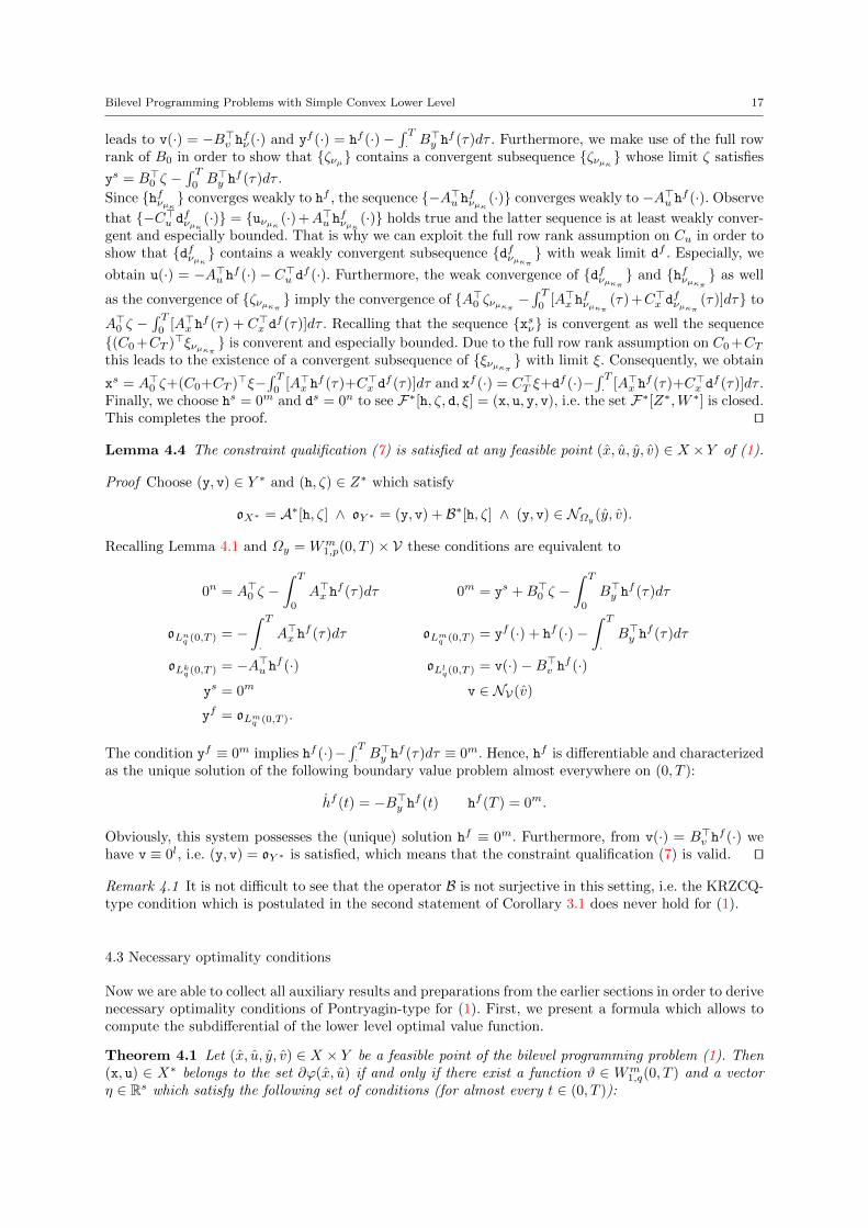
Lemma 4.4 The constraint qualification (7) is satisfied at any feasible point (x, u, y, v) ∈ X ×Y of (1).
Proof Choose (y, v) ∈ Y ∗ and (h, ζ) ∈ Z∗ which satisfy
oX∗ = A∗[h, ζ] ∧ oY ∗ = (y, v) + B∗[h, ζ] ∧ (y, v) ∈ NΩy (y, v).
Recalling Lemma 4.1 and Ωy = Wm1,p(0, T )× V these conditions are equivalent to
0n = A>0 ζ −∫ T
0
A>x hf (τ)dτ 0m = ys +B>0 ζ −
∫ T
0
B>y hf (τ)dτ
oLnq (0,T ) = −∫ T
·A>x h
f (τ)dτ oLmq (0,T ) = yf (·) + hf (·)−∫ T
·B>y h
f (τ)dτ
oLkq (0,T ) = −A>u hf (·) oLlq(0,T ) = v(·)−B>v hf (·)
ys = 0m v ∈ NV(v)
yf = oLmq (0,T ).
The condition yf ≡ 0m implies hf (·)−∫ T· B
>y h
f (τ)dτ ≡ 0m. Hence, hf is differentiable and characterizedas the unique solution of the following boundary value problem almost everywhere on (0, T ):
hf (t) = −B>y hf (t) hf (T ) = 0m.
Obviously, this system possesses the (unique) solution hf ≡ 0m. Furthermore, from v(·) = B>v hf (·) we
have v ≡ 0l, i.e. (y, v) = oY ∗ is satisfied, which means that the constraint qualification (7) is valid. ut
Remark 4.1 It is not difficult to see that the operator B is not surjective in this setting, i.e. the KRZCQ-type condition which is postulated in the second statement of Corollary 3.1 does never hold for (1).
4.3 Necessary optimality conditions
Now we are able to collect all auxiliary results and preparations from the earlier sections in order to derivenecessary optimality conditions of Pontryagin-type for (1). First, we present a formula which allows tocompute the subdifferential of the lower level optimal value function.
Theorem 4.1 Let (x, u, y, v) ∈ X × Y be a feasible point of the bilevel programming problem (1). Then(x, u) ∈ X∗ belongs to the set ∂ϕ(x, u) if and only if there exist a function ϑ ∈ Wm
1,q(0, T ) and a vectorη ∈ Rs which satisfy the following set of conditions (for almost every t ∈ (0, T )):
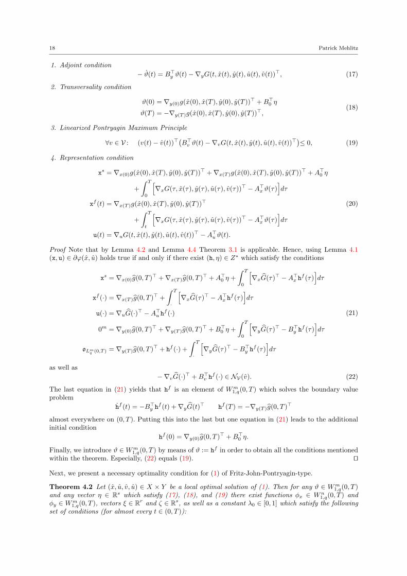
18 Patrick Mehlitz
1. Adjoint condition
− ϑ(t) = B>y ϑ(t)−∇yG(t, x(t), y(t), u(t), v(t))>, (17)
2. Transversality condition
ϑ(0) = ∇y(0)g(x(0), x(T ), y(0), y(T ))> +B>0 η
ϑ(T ) = −∇y(T )g(x(0), x(T ), y(0), y(T ))>,(18)
3. Linearized Pontryagin Maximum Principle
∀v ∈ V : (v(t)− v(t))>(B>v ϑ(t)−∇vG(t, x(t), y(t), u(t), v(t))>
)≤ 0, (19)
4. Representation condition
xs = ∇x(0)g(x(0), x(T ), y(0), y(T ))> +∇x(T )g(x(0), x(T ), y(0), y(T ))> +A>0 η
+
∫ T
0
[∇xG(τ, x(τ), y(τ), u(τ), v(τ))> −A>x ϑ(τ)
]dτ
xf (t) = ∇x(T )g(x(0), x(T ), y(0), y(T ))>
+
∫ T
t
[∇xG(τ, x(τ), y(τ), u(τ), v(τ))> −A>x ϑ(τ)
]dτ
u(t) = ∇uG(t, x(t), y(t), u(t), v(t))> −A>u ϑ(t).
(20)
Proof Note that by Lemma 4.2 and Lemma 4.4 Theorem 3.1 is applicable. Hence, using Lemma 4.1(x, u) ∈ ∂ϕ(x, u) holds true if and only if there exist (h, η) ∈ Z∗ which satisfy the conditions
xs = ∇x(0)g(0, T )> +∇x(T )g(0, T )> +A>0 η +
∫ T
0
[∇xG(τ)> −A>x hf (τ)
]dτ
xf (·) = ∇x(T )g(0, T )> +
∫ T
·
[∇xG(τ)> −A>x hf (τ)
]dτ
u(·) = ∇uG(·)> −A>u hf (·)
0m = ∇y(0)g(0, T )> +∇y(T )g(0, T )> +B>0 η +
∫ T
0
[∇yG(τ)> −B>y hf (τ)
]dτ
oLmq (0,T ) = ∇y(T )g(0, T )> + hf (·) +
∫ T
·
[∇yG(τ)> −B>y hf (τ)
]dτ
(21)
as well as
−∇vG(·)> +B>v hf (·) ∈ NV(v). (22)
The last equation in (21) yields that hf is an element of Wm1,q(0, T ) which solves the boundary value
problem
hf (t) = −B>y hf (t) +∇yG(t)> hf (T ) = −∇y(T )g(0, T )>
almost everywhere on (0, T ). Putting this into the last but one equation in (21) leads to the additionalinitial condition
hf (0) = ∇y(0)g(0, T )> +B>0 η.
Finally, we introduce ϑ ∈Wm1,q(0, T ) by means of ϑ := hf in order to obtain all the conditions mentioned
within the theorem. Especially, (22) equals (19). ut
Next, we present a necessary optimality condition for (1) of Fritz-John-Pontryagin-type.
Theorem 4.2 Let (x, u, v, u) ∈ X × Y be a local optimal solution of (1). Then for any ϑ ∈ Wm1,q(0, T )
and any vector η ∈ Rs which satisfy (17), (18), and (19) there exist functions φx ∈ Wn1,q(0, T ) and
φy ∈ Wm1,q(0, T ), vectors ξ ∈ Rr and ζ ∈ Rs, as well as a constant λ0 ∈ [0, 1] which satisfy the following
set of conditions (for almost every t ∈ (0, T )):
Bilevel Programming Problems with Simple Convex Lower Level 19
1. Adjoint condition
−φx(t) = C>x φx(t)− λ0 · ∇xF (t, x(t), y(t), u(t), v(t))> +A>x φy(t)− (1− λ0) ·A>x ϑ(t)
−φy(t) = B>y φy(t)−∇y(λ0 · F + (1− λ0) ·G
)(t, x(t), y(t), u(t), v(t))>,
(23)
2. Transversality condition
φx(0) = λ0 · ∇x(0)f(x(0), x(T ), y(0), y(T ))> +A>0 ζ − (1− λ0) ·A>0 η + C>0 ξ
φy(0) = ∇y(0)(λ0 · f + (1− λ0) · g
)(x(0), x(T ), y(0), y(T ))> +B>0 ζ
φx(T ) = −λ0 · ∇x(T )f(x(0), x(T ), y(0), y(T ))> − C>T ξφy(T ) = −∇y(T )
(λ0 · f + (1− λ0) · g
)(x(0), x(T ), y(0), y(T ))>,
(24)
3. Linearized Pontryagin Maximum Principle
∀u ∈ U : (u(t)− u(t))>(C>u φx(t) +A>u φy(t)− (1− λ0) ·A>u ϑ(t)
−λ0 · ∇uF (t, x(t), y(t), u(t), v(t))>)≤ 0
∀v ∈ V : (v(t)− v(t))>(B>v φy(t)−∇v
(λ0 · F + (1− λ0) ·G
)(t, x(t), y(t), u(t), v(t))>
)≤ 0.
(25)
Proof Due to Lemma 4.2, Lemma 4.3, and Lemma 4.4 Theorem 3.2 is applicable. Hence, recalling theproof of Theorem 4.1 and Lemma 4.1, for any (h, η) ∈ Z∗ which satisfy the last two conditions in (21),and (22) we find (d, ξ) ∈W ∗, (k, ζ) ∈ Z∗, and λ0 ∈ [0, 1] which satisfy
0n = λ0(∇x(0)f(0, T )> +∇x(T )f(0, T )>
)+A>0
(ζ − (1− λ0)η
)+(C0 + CT )>ξ
+
∫ T
0
[λ0 · ∇xF (τ)> −A>x
(kf (τ)− (1− λ0)hf (τ)
)−C>x df (τ)
]dτ
oLnq (0,T ) = λ0 · ∇x(T )f(0, T )> + C>T ξ + df (·)
+
∫ T
·
[λ0 · ∇xF (τ)> −A>x
(kf (τ)− (1− λ0)hf (τ)
)−C>x df (τ)
]dτ
0m = λ0(∇y(0)f(0, T )> +∇y(T )f(0, T )>
)+(1− λ0)
(∇y(0)g(0, T )> +∇y(T )g(0, T )>
)+B>0 ζ
+
∫ T
0
[λ0 · ∇yF (τ)> + (1− λ0) · ∇yG(τ)> −B>y kf (τ)
]dτ
oLmq (0,T ) = λ0 · ∇y(T )f(0, T )> + (1− λ0) · ∇y(T )g(0, T )> + kf (·)
+
∫ T
·
[λ0 · ∇yF (τ)> + (1− λ0) · ∇yG(τ)> −B>y kf (τ)
]dτ
(26)
as well as
−λ0 · ∇uF (·)> +A>u(kf (·)− (1− λ0)hf (·)
)+C>u d
f (·) ∈ NU (u)
−λ0 · ∇vF (·)> − (1− λ0) · ∇vG(τ)> +B>v kf (·) ∈ NV(v).
(27)
From the proof of Theorem 4.1 we know that (h, η) satisfy the last two conditions in (21), and (22) ifand only if ϑ := hf and η satisfy (17), (18), and (19). That means we only have to transform (26) and(27) into the above necessary optimality conditions replacing hf by ϑ in order to verify the statement ofthe theorem.The second and the forth equation in (26) yield df ∈Wn
1,q(0, T ) as well as kf ∈Wm1,q(0, T ) and the latter
functions solve the following boundary value problem:
df (t) = −C>x df (t) + λ0 · ∇xF (t)> −A>x kf (t) + (1− λ0) ·A>x ϑ(t)
kf (t) = −B>y kf (t) + λ0 · ∇yF (t)> + (1− λ0)∇yG(t)>
df (T ) = −λ0 · ∇x(T )f(0, T )> − C>T ξ
kf (T ) = −λ0 · ∇y(T )f(0, T )> − (1− λ0) · ∇y(T )g(0, T )>.
20 Patrick Mehlitz
The first and the third equation from (26) now lead to the following additional initial constraints:
df (0) = λ0 · ∇x(0)f(0, T )> +A>0 ζ − (1− λ0) ·A>0 η + C>0 ξ
kf (0) = λ0 · ∇y(0)f(0, T )> + (1− λ0) · ∇y(0)g(0, T )> +B>0 ζ.
We introduce φx ∈ Wn1,q(0, T ) and φy ∈ Wm
1,q(0, T ) by means of φx := df and φy := kf and put thesefunctions into the above boundary value problem and into (27) in order to obtain the necessary optimalityconditions of the theorem. ut
Note that for λ0 = 0 the upper level objective function is eliminated from the above system (23), (24),(25) while all the conditions which characterize φy and ζ become the same conditions which characterizeϑ and η in Theorem 4.1, i.e. the lower level optimality conditions (17), (18), and (19). Hence, if the point(x, u, y, v) ∈ X × Y is feasible for (1), then for any ϑ ∈ Wm
1,q(0, T ) and η ∈ Rs which satisfy (17), (18),and (19) one could choose λ0 := 0, φx ≡ 0n, ξ := 0r, φy := ϑ, ζ := η in order to satisfy (23), (24), and(25).That means the above necessary optimality conditions hold at any feasible point of (1) which makesthem not pretty useful as long as the choice λ0 = 0 is allowed. Of course one could try to find minimizercandidates of (1) by checking the above system only for λ0 ∈ (0, 1] but this is not really a trustworthapproach since this way one could exclude somehow irregular minimizers.The theorem below presents optimality conditions which always contain information on the upper levelobjective by making the additional assumption on (1) to be partially calm at the considered local optimalsolution.
Theorem 4.3 Let (x, u, y, v) ∈ X × Y be a local optimal solution of (1) where the latter problem ispartially calm. Then there is a constant α > 0 such that for any function ϑ ∈Wm
1,q(0, T ) and any η ∈ Rswhich satisfy (17), (18), and (19) there exist functions φx ∈ Wn
1,q(0, T ) and φy ∈ Wm1,q(0, T ) as well as
vectors ξ ∈ Rr and ζ ∈ Rs which satisfy the following set of conditions (for almost every t ∈ (0, T )):
1. Adjoint condition
−φx(t) = C>x φx(t)−∇xF (t, x(t), y(t), u(t), v(t))> +A>x φy(t)− α ·A>x ϑ(t)
−φy(t) = B>y φy(t)−∇y(F + α ·G
)(t, x(t), y(t), u(t), v(t))>,
(28)
2. Transversality condition
φx(0) = ∇x(0)f(x(0), x(T ), y(0), y(T ))> +A>0 ζ − α ·A>0 η + C>0 ξ
φy(0) = ∇y(0)(f + α · g
)(x(0), x(T ), y(0), y(T ))> +B>0 ζ
φx(T ) = −∇x(T )f(x(0), x(T ), y(0), y(T ))> − C>T ξφy(T ) = −∇y(T )
(f + α · g
)(x(0), x(T ), y(0), y(T ))>,
(29)
3. Linearized Pontryagin Maximum Principle
∀u ∈ U : (u(t)− u(t))>(C>u φx(t) +A>u φy(t)− α ·A>u ϑ(t)
−∇uF (t, x(t), y(t), u(t), v(t))>)≤ 0
∀v ∈ V : (v(t)− v(t))>(B>v φy(t)−∇v
(F + α ·G
)(t, x(t), y(t), u(t), v(t))>
)≤ 0.
(30)
Proof The proof is similar to the argumentation in the proof of Theorem 4.2 using Theorem 3.3. ut
Finally, we can state necessary optimality conditions for the corresponding minimax problem.
Theorem 4.4 Let (x, u, y, v) be a local optimal solution of (1) where f := −g and F := −G hold true.Then for any function ϑ ∈ Wm
1,q(0, T ) and any η ∈ Rs which satisfy (17), (18), and (19) there exist afunction φx ∈ Wn
1,q(0, T ) as well as a vector ξ ∈ Rr which satisfy the following set of conditions (foralmost every t ∈ (0, T )):
1. Adjoint condition
− φx(t) = C>x φx(t) +∇xG(t, x(t), y(t), u(t), v(t))> −A>x ϑ(t), (31)
Bilevel Programming Problems with Simple Convex Lower Level 21
2. Transversality condition
φx(0) = −∇x(0)g(x(0), x(T ), y(0), y(T ))> −A>0 η + C>0 ξ
φx(T ) = ∇x(T )g(x(0), x(T ), y(0), y(T ))> − C>T ξ,(32)
3. Linearized Pontryagin Maximum Principle
∀u ∈ U : (u(t)− u(t))>(C>u φx(t)−A>u ϑ(t) +∇uG(t, x(t), y(t), u(t), v(t))>
)≤ 0. (33)
Proof Similar as mentioned in the proof of the first statement of Corollary 3.1 one obtains these necessaryoptimality conditions by fixing f = −g, F = −G, and α = 1 in (28), (29), and (30). Writing this systemdown one obtains φy ≡ 0m from the differential equation −φy(t) = B>y φy(t) and the corresponding
terminal condition φy(T ) = 0m. This leads to B>0 ζ = 0m which implies ζ = 0s by the full row rankassumption on the matrix B0. ut
We want to close this paper with two small remarks on our results.
Remark 4.2 The necessary optimality conditions we obtained in Theorem 4.4 are the same as postulatedfor the general case in the second statement of Corollary 3.1. Observe that due to Remark 4.1 this resultis not applicable to (1) directly.
Remark 4.3 Let (x, u, y, v) ∈ X × Y be a local optimal solution of (1). Observe that the statements ofTheorem 4.2, Theorem 4.3, and Theorem 4.4 are only useful provided there exist a function ϑ ∈Wm
1,q(0, T )and a vector η ∈ Rs which satisfy the conditions (17), (18), and (19), i.e., by Theorem 4.1, if and only if∂ϕ(x, u) is nonempty. This condition always holds for (x, u) ∈ ri(dom(ϕ)).
References
1. Albrecht, S., Leibold, M., Ulbrich, M.: A bilevel optimization approach to obtain optimal cost functions for humanarm movements. Control and Optimization 2(1), 105–127 (2012)
2. Benita, F., Dempe, S., Mehlitz, P.: Bilevel Optimal Control Problems with Pure State Constraints and Finite-dimensional Lower Level. Preprint TU Bergakademie Freiberg (2015)
3. Benita, F., Mehlitz, P.: Bilevel optimal control with final-state-dependent finite-dimensional lower level. Preprint TUBergakademie Freiberg (2014)
4. Bonnans, J.F., Shapiro, A.: Perturbation Analysis of Optimization Problems. Springer-Verlag, New York, Berlin,Heidelberg (2000)
5. Bonnel, H., Morgan, J.: Semivectorial Bilevel Convex Optimal Control Problems: Existence Results. SIAM Journal onControl and Optimization 50(6), 3224–3241 (2012)
6. Bonnel, H., Morgan, J.: Optimality conditions for semivectorial bilevel convex optimal control problems. In: D.H.Bailey, H.H. Bauschke, P. Borwein, F. Garvan, M. Thera, J.D. Vanderwerff, H. Wolkowicz (eds.) Computational andAnalytical Mathematics, Springer Proceedings in Mathematics and Statistics, vol. 50, pp. 45–78. Springer New York(2013)
7. Chieu, N.H., Kien, B.T., Toan, N.T.: Further Results on Subgradients of the Value Function to a Parametric OptimalControl Problem. Journal of Optimization Theory and Applications (2011). DOI 10.1007/s10957-011-9933-0
8. Dempe, S.: Foundations of Bilevel Programming. Kluwer Academic Publishers, Dordrecht (2002)9. Dempe, S., Dutta, J., Mordukhovich, B.S.: New necessary optimality conditions in optimistic bilevel programming.
Optimization 56(5), 577–604 (2007)10. Dempe, S., Kalashnikov, V.V., Rıos-Mercado, R.Z.: Discrete bilevel programming: Application to a natural gas cash-out
problem. European Journal of Operational Research 166(2), 469–488 (2005)11. Dempe, S., Mehlitz, P.: Lipschitz continuity of the optimal value function in parametric optimization. Journal of Global
Optimization pp. 1–15 (2014). DOI 10.1007/s10898-014-0169-z12. Dempe, S., Zemkoho, A.B.: The bilevel programming problem: reformulations, constraint qualications and optimality
conditions. Mathematical Programming 138, 447–473 (2013)13. Demyanov, V.F., Rubinov, A.M.: Quasidifferentiability and Related Topics. Springer, New York (2000)14. Fiacco, A., Kyparisis, J.: Convexity and concavity properties of the optimal value function in nonlinear parametric
programming. Journal of Optimization Theory and Applications 48(1), 95–126 (1986)15. Fisch, F., Lenz, J., Holzapfel, F., Sachs, G.: On the Solution of Bilevel Optimal Control Problems to Increase the
Fairness of Air Race. Journal of Guidance, Control and Dynamics 35, 1292–1298 (2012)16. Henrion, R., Surowiec, T.: On calmness conditions in convex bilevel programming. Applicable Analysis 90(6), 951–970
(2011)17. Ioffe, A.D., Tichomirov, V.M.: Theory of Extremal Problems. North-Holland Publishing Company, Amsterdam, New
York, Oxford (1979)18. Kalashnikov, V.V., Dempe, S., Perez-Valdez, G.A., Kalashnykova, N.I.: Natural gas cash-out problem: Solution with
bilevel programming tools. In: The 2011 New Orleans International Academic Conference. New Orleans, LouisianaUSA (2011)
22 Patrick Mehlitz
19. Kalashnikov, V.V., Perez-Valdez, G.A., Kalashnykova, N.I.: A linearization approach to solve the natural gas bilevelproblem. Annals of Operations Research 181(1), 423–442 (2010)
20. Kalashnikov, V.V., Perez-Valdez, G.A., Tomasgard, A., Kalashnykova, N.I.: Natural gas cash-out problem: Bilevelstochastic optimization approach. European Journal of Operational Research 206(1), 18–33 (2010)
21. Kalashnikov, V.V., Rıos-Mercado, R.Z.: A natural gas cash-out problem: A bilevel programming framework and apenalty function method. Optimization and Engineering 7(4), 403–420 (2006)
22. Knauer, M., Buskens, C.: Hybrid Solution Methods for Bilevel Optimal Control Problems with Time DependentCoupling. In: M. Diehl, F. Glineur, E. Jarlebring, W. Michiels (eds.) Recent Advances in Optimization and itsApplications in Engineering, pp. 237–246. Springer Berlin Heidelberg (2010)
23. Knauer, M., Buskens, C., Lasch, P.: Real-Time Solution of Bi-Level Optimal Control Problems. PAMM 5(1), 749–750(2005)
24. Kurcyusz, S., Zowe, J.: Regularity and Stability for the Mathematical Programming Problem in Banach Spaces. AppliedMathematics and Optimization 5, 49–62 (1979)
25. Mombaur, K., Truong, A., Laumond, J.P.: From human to humanoid locomotionan inverse optimal control approach.Autonomous Robots 28(3), 369–383 (2010)
26. Mordukhovich, B.S.: Variational Analysis and Generalized Differentiation I and II. Springer-Verlag, Berlin, Heidelberg(2006)
27. Mordukhovich, B.S., Nam, N.M.: Variational stability and marginal functions via generalized differentiation. Mathe-matics of Operations Research 30(4), 800–816 (2005)
28. Mordukhovich, B.S., Nam, N.M., Yen, N.D.: Frechet subdifferential calculus and optimality conditions in nondifferen-tiable programming. Optimization 55(5-6), 685–708 (2006)
29. Mordukhovich, B.S., Nam, N.M., Yen, N.D.: Subgradients of marginal functions in parametric mathematical program-ming. Mathematical Programming 116, 369–396 (2009)
30. Robinson, S.: Stability theory for systems of inequalities, Part II: Differentiable nonlinear systems. SIAM Journal onNumerical Analysis 13(4), 497–513 (1976)
31. Wachsmuth, G.: Mathematical Programs with Complementarity Constraints in Banach Spaces. Journal of OptimizationTheory and Applications pp. 1–28 (2014). DOI 10.1007/s10957-014-0695-3
32. Werner, D.: Funktionalanalysis. Springer-Verlag, Berlin, Heidelberg (1995)33. Ye, J.J.: Optimal strategies for bilevel dynamic problems. SIAM Journal on Optimization and Control 35(2), 512–531
(1997)34. Ye, J.J., Zhu, D.L.: Optimality conditions for bilevel programming problems. Optimization 33, 9–27 (1995)