Assessing the Fit of a Small Open-Economy DSGE Model for the Brazilian Economy

Fernando de Menezes Linardi

April, 2016

424

ISSN 1518-3548 CGC 00.038.166/0001-05

Working Paper Series Brasília n. 424 April 2016 p. 1-39

Working Paper Series Edited by Research Department (Depep) – E-mail: workingpaper@bcb.gov.br Editor: Francisco Marcos Rodrigues Figueiredo – E-mail: francisco-marcos.figueiredo@bcb.gov.br Editorial Assistant: Jane Sofia Moita – E-mail: jane.sofia@bcb.gov.br Head of Research Department: Eduardo José Araújo Lima – E-mail: eduardo.lima@bcb.gov.br The Banco Central do Brasil Working Papers are all evaluated in double blind referee process. Reproduction is permitted only if source is stated as follows: Working Paper n. 424. Authorized by Altamir Lopes, Deputy Governor for Economic Policy. General Control of Publications Banco Central do Brasil

Comun/Dipiv/Coivi

SBS – Quadra 3 – Bloco B – Edifício-Sede – 14º andar

Caixa Postal 8.670

70074-900 Brasília – DF – Brazil

Phones: +55 (61) 3414-3710 and 3414-3565

Fax: +55 (61) 3414-1898

E-mail: editor@bcb.gov.br

The views expressed in this work are those of the authors and do not necessarily reflect those of the Banco Central or its members. Although these Working Papers often represent preliminary work, citation of source is required when used or reproduced. As opiniões expressas neste trabalho são exclusivamente do(s) autor(es) e não refletem, necessariamente, a visão do Banco Central do Brasil. Ainda que este artigo represente trabalho preliminar, é requerida a citação da fonte, mesmo quando reproduzido parcialmente. Citizen Service Division Banco Central do Brasil

Deati/Diate

SBS – Quadra 3 – Bloco B – Edifício-Sede – 2º subsolo

70074-900 Brasília – DF – Brazil

Toll Free: 0800 9792345

Fax: +55 (61) 3414-2553

Internet: <http//www.bcb.gov.br/?CONTACTUS>

  

Assessing the Fit of a Small Open-Economy DSGE Model for the Brazilian Economy*

Fernando de Menezes Linardi**

Abstract

The Working Papers should not be reported as representing the views of the Banco Central do Brasil. The views expressed in the papers are those of the author(s) and do not

necessarily reflect those of the Banco Central do Brasil.

This paper estimates a small open-economy dynamic stochastic general equilibrium (DSGE) model using Brazil´s economy data for the inflation-targeting period. The model includes a number of shocks that are important to explain the macroeconomic fluctuations of emerging markets economies. Then the empirical fit of different specifications of the model is tested in a Bayesian framework. The potential model misspecification is also assessed by comparing it to a more general reference model using the DSGE-VAR approach. The results show that the model with no price indexation fits the data better than the fully specified one. The DSGE-VAR approach indicated some degree of misspecification in the stylized small open-economy model. Keywords: Bayesian estimation, DSGE-VAR approach, model misspecification, small open-economy DSGE models. JEL Classification: C11, C51, E52, F41.

                                                            * The author thanks Robert Kollmann for suggestions that have helped improve the paper. ** Central Bank of Brazil. E-mail: fernando.linardi@bcb.gov.br.  

3

1 Introduction

In this paper we estimate a Dynamic Stochastic General Equilibrium (DSGE)

model using Brazilian economy data for the period of inflation targeting regime

followed by the Central Bank of Brazil since 1999. The model includes shocks to terms

of trade, risk premium and world interest rates that are important to explain the

macroeconomic volatility of emerging market economies (EMEs). The main objective

is to assess in a Bayesian framework the empirical fit of different specifications of the

small open economy model.

Currently, estimated DSGE models are widely used for empirical

macroeconomics research and policy analysis. Following the influential papers of

Christiano et al. (2005) and Smets and Wouters (2003) many works have developed

DSGE models including a number of nominal and real rigidities that have proved to be

crucial in fitting models to data. In general, they show that estimated DSGE models are

able to perform better than standard VARs or to match the economic dynamics.

Despite the advances in economic modeling, the evaluation of model´s fit is still

an important issue in the econometric analysis of DSGE models. Although they may

provide a multivariate stochastic process representation for the data which is

theoretically coherent, some models impose very strong restrictions on observed time

series which may be rejected against less restrictive specifications such as a VAR (An

and Schorfheide, 2007).

Significant contributions to the development of general equilibrium models for

open economies were made by, among others, Kollmann (2002), Schmitt-Grohé and

Uribe (2001) and Galí and Monacelli (2005). Kollmann (2002) develops a small open

economy model assuming monopolistic competition and staggered price setting to

compute the effect of the monetary policy regime on welfare and business cycles. Using

a small open economy model with sticky prices calibrated to the Mexican economy,

Schmitt-Grohé and Uribe (2001) compare the wealfare costs of business cycles in a

dollarized economy to three alternative monetary policy regimes.

Galí and Monacelli (2005) present a calibrated DSGE model for a small open

economy with Calvo type staggered price-setting, and use it as a framework for

analyzing the properties and macroeconomic implications of three alternative monetary

policy rules. Two of the monetary policy regimes considered are stylized Taylor-type

4

rules and the other one is a nominal exchange rate pegging. They model the world

economy as a continuum of small open economies represented by the unit interval and

domestic policy decisions of each economy do not have any impact on the rest of the

world. While different economies are subject to imperfectly correlated productivity

shocks, the authors assume that they share identical preferences, technology, and market

structure.

There is a vast literature on estimating small open-economy models using

Bayesian methods. For instance, Adalfson et al. (2007) develop a DSGE model for an

open economy, and estimate it on Euro area data using Bayesian estimation techniques.

Following Christiano et al. (2005), a number of nominal and real frictions such as sticky

prices, sticky wages, variable capital utilization, capital adjustment costs and habit

persistence are included in the theoretical model. Following Smets and Wouters (2002)

they also allow for incomplete exchange rate pass-through in both the import and export

sectors by including nominal price rigidities.

Lubik and Schorfheide (2007) try to answer the question of to what extent

central banks include exchange rates in the process of formulating monetary policy.

They apply Bayesian estimation techniques to four small open economies (Australia,

Canada, New Zealand and the U.K) using a simplified version of Galí and Monacelli

(2005) model. The main finding of the paper is that the central banks of Australia, New

Zealand, and the U.K. did not explicitly respond to exchange rates over the last two

decades. However, the Bank of Canada did. According to the authors, this finding is

robust over different specifications of the monetary policy reaction function, such as

expected inflation targeting.

Justiniano and Preston (2010b) analyze optimal policy design in an estimated

small open economy for Australia, Canada and New Zealand taking also in account the

consequences of model uncertainty. Their aim is to verify whether policies in a class of

generalized Taylor rules optimally respond to exchange rate variations as predicted by

theory. Their analysis is done using extensions of the small open-economy framework

proposed by Gali and Monacelli (2005) and Monacelli (2005), and considering a small–

large country pair, rather than a continuum of small open economies. In this case, a

small and large country each specializes in the production of a continuum of goods

subject to imperfect competition and price rigidities. Imports are subject to local

5

currency pricing giving rise to deviations from the law of one price. Differently from

Gali and Monacelli (2005) they consider incomplete asset markets in addition to other

rigidities such as indexation and habit formation as well as a large set of disturbances to

fit the model to the data.

Finally, applying Bayesian methods Kam et al. (2009) also estimate the

macroeconomic policy objectives of the central banks of Australia, Canada, and New

Zealand within the context of a small open economy DSGE model. Using a stylized

economy model similar to Justiniano and Preston (2010b) they find that none of the

central banks is concerned for stabilizing the real exchange rate. Although all of them

are concerned for minimizing the volatility in the change of the nominal interest rate.

These results are contrary to Lubik and Schorfheide (2007) who find some evidence that

Canada does respond to changes in the exchange rate. According to them, the difference

is explained by the lack of an endogenous terms of trade specification and the lack of

imperfect pass-through of nominal exchange rate changes into domestic import prices.

In the case of Brazil, Silveira (2008) used a Bayesian approach to estimate and

compare alternative model specifications for the Brazilian economy with respect to two

endogenous persistence mechanisms: habit formation and price indexation. Estimating a

model based in Galí and Monacelli (2005) he concluded that both mechanisms are

relevant to explain the dynamic of the economy during the period analyzed, although

the evidence is less robust to price indexation.

Castro et al. (2011) developed and estimated a DSGE model for the Brazilian

economy which is used as part of the macroeconomic modeling framework at the

Central Bank of Brazil. They model a small open economy combining standard features

of DSGE models as wage and price rigidities with specific features of the Brazilian

economy. They concluded based on model evaluation techniques that the model can be

used as a tool for policy analysis and forecasting.

Palma and Portugal (2014) based on the work of Kam et al. (2009) estimated the

preferences of the Central Bank of Brazil after the inflation targeting regime. The

authors considered that the central bank minimizes a loss function, taking into account

deviation of inflation from its target, output stabilization, interest rate smoothing and the

exchange rate. They concluded that the monetary authority in the period was concerned

6

with stabilization of inflation, interest rate smoothing, stabilization of output and

exchange rate, following this order of importance.

We present a model for a small open economy based on Kam et al. (2009) and

estimate it on Brazilian data using Bayesian methods. Differently from Palma and

Portugal (2014) who investigate the policy objectives of the Central Bank of Brazil we

are mainly interested in assessing the fit of the model. The model includes a number of

nominal and real frictions as habit persistence, price indexation and deviations from the

law of one price. It nests a number of different specifications of the small open economy

model, therefore it is possible to examine the relative fit across a range of models using

posterior odds ratios. In addition, the ability of the fully specified model to fit particular

second order moments of the data is discussed.

Then we investigate the potential model misspecification implied by invalid

cross-coefficient restrictions on the time series representation generated by the DSGE

model. These invalid restrictions manifest in poor out-of-sample fit relative to more

densely parameterized reference models such as VARs (An and Schorfheide, 2007).

The misspecification of the small open economy model was analyzed by

Justiniano and Preston (2010b). They found that the estimated model of the Canadian

economy cannot account for the significant influence of the U.S. shocks on economic

fluctuations of Canada that have been verified by many empirical works. Del Negro et

al. (2007) found evidence of misspecification in a large-scale new Keynesian model.

However, accounting for misspecification by relaxing the DSGE model restrictions does

not significantly alter the responses to monetary policy and technology shocks. Despite

its deficiencies, they concluded that the DSGE model can generate realistic predictions

of the effects of unanticipated changes in monetary policy and technology shocks.

In our work the model misspecification is assessed using the DSGE-VAR

approach developed by Del Negro and Schorfheide (2004) and extended in Del Negro et

al. (2007). In this approach a VAR is used as an approximating model for the DSGE

model. The cross-coefficient restrictions implied by the DSGE model are systematically

relaxed and the model´s fit is assessed. Deviations of the VAR parameters from the

restrictions are interpreted as DSGE model misspecification. This approach provide a

reliable benchmark to evaluate the model´s misspecification given that posterior odds of

a DSGE model versus a VAR with a fairly diffuse prior do not provide a robust

7

assessment of fit. A VAR with a diffuse prior is likely to be rejected even against a

misspecified DSGE model (An and Schorfheide, 2007).

Del Negro and Schorfheide (2008) use the DSGE-VAR approach to assess the

model´s robustness to the presence of model misspecification in the study of the policy

rule followed by the Central Bank of Chile. They analyze the dynamic response of

inflation to domestic and external shocks and the change in the response of inflation

under different policy parameters. Bäurle and Menz (2008) use the same framework to

study the transmission of monetary shocks in Switzerland. They assess whether the

central bank reacts to changes in the nominal exchange rate.

Gupta and Steinbach (2013) develop a small open economy DSGE-VAR model

of the South Africa economy and use it to forecast output growth, inflation and short

term interest rates. Forecast performance of the model is compared to an independently

estimated DSGE model and to VAR and BVAR models. They conclude that the BVAR

model provides the best forecasts of the three variables. Using data from the New

Zealand economy Lees et al. (2011) also found that the BVAR out-performs both the

DSGE-VAR and the central bank´s own forecasts. Finally, Marcellino and Rychalovska

(2014) develop a two-region DSGE model of an open economy within the European

Monetary Union and apply the DSGE-VAR approach to study the empirical validity of

the restrictions implied by the DSGE model.

The paper is organized as follows. Section 2 discusses some issues in estimating

small open economy models for emerging market economies. In section 3 the

theoretical model is presented. In section 4 and 5 it is outlined the estimation

methodology and the dataset used for the estimation. In section 6, the main results are

discussed. Section 7 concludes.

2 Estimation of DSGE models for emerging market economies (EMEs)

Estimation of DSGE models for EMEs is challenge considering that their

business cycles are characterized by large volatility and current account reversals

("sudden stops"). Aguiar and Gopinath (2007) explain that their trade balance is

strongly countercyclical as compared to developed markets and consumption is much

more volatile than income. In addition, income growth and net exports are twice as

volatile in EMEs. Despite their peculiarities, the authors show that a standard real

business cycle model (RBC) can reproduce to a large extent the business cycle features

8

of EMEs. Their model is driven by a transitory and a permanent shock to the trend

growth rate.

On the other hand, García-Cicco et al. (2010) find that, when estimated over a

very long sample (1900-2005), the RBC model driven by permanent and transitory

productivity shocks could not explain adequately observed business cycles in Argentina

and Mexico along a number of dimensions such as trade balance-to-output ratio or the

observed excess volatility in consumption. They further estimate an augmented model

that incorporates debt elasticity of the country interest rate, country-premium shocks,

preference shocks and domestic spending shocks. They conclude that the augmented

model provides an adequate explanation of the Argentine business cycle.

Other works have included a number of disturbances that are important to

explain the business cycle variations of EMEs. Given that many of them are exporters

of a few primary commodities, shocks to the terms of trade − ratio of the price of

imports to exports − may play an important role in explaining output fluctuations. Hove

et al. (2015) evaluate the optimal monetary policy responses to terms of trade shocks in

commodity dependent EMEs. Devereux et al. (2006) compare alternative monetary

policy rules in a model of an EME that experiences external shocks to world interest

rates and the terms of trade.

Furthermore, there are evidences that changes in the cost of borrowing affect

significantly EMEs. Shocks could be caused by changes in world interest rates or

country risk premiums. Many studies have emphasized the role of movements in U.S.

interest rates and country spreads in driving business cycles in EMEs. Uribe and Yue

(2006) conclude based on a panel VAR of seven EMEs that U.S. interest rate shocks

explain 20% of the output variance and about 12% can be explained by country

premium shocks.

Considering this, in addition to monetary policy and technology shocks, our

model includes shocks to the terms of trade, risk premium and world interest rates. We

estimate the model for the Brazilian economy using data on output growth, inflation,

exchange rate and interest rates. After the launch of the Plano Real in 1994 which

changed the currency and ended a period of high inflation in Brazil the monetary policy

was based on exchange rate peg. In 1999 the floating exchange rate regime was adopted

and in the same year the inflation targeting regime was officially implemented. Hence,

9

we decided to use data only for the inflation targeting period which unfortunately it is

not a long sample.

3 A simple small open economy model

The stylized economy is analogous to the open economy model presented in

Kam et al. (2009). We consider the case of a small open economy where households are

assumed to maximize a utility function over an infinite life horizon. The household

derives utility from leisure and consumption relative to an external habit parameter.

There are two types of firms in the economy: domestic goods firms and importing firms.

The continuum of monopolistically competitive domestic goods firms produce

differentiated goods and operate a linear production technology. The continuum of

import retail firms add markups to goods imported at world prices.

Sticky price is introduced to the model following Calvo, where some of the

firms choose their prices optimally and the other part chooses according to past

inflation. Furthermore, in determining the domestic currency price of the imported

good, retail firms are assumed to be monopolistically competitive giving rise to

deviations from the law of one price. Finally, monetary policy is assumed to be

conducted according to a Taylor-type rule and fiscal policy is specified as a zero debt

policy.

The foreign economy is exogenous to the domestic economy and for simplicity

it is assumed that output, inflation and real interest rate of the foreign economy are

given by uncorrelated AR(1) processes.

3.1. Household sector

The economy is inhabited by a representative household who maximizes an

intertemporal utility function given by:

∑ , (1)

where βt is the discount factor, σ and φ are the inverse elasticities of intertemporal

substitution and labor supply, respectively. Nt is the labor supply and Ht = hCt-1 is an

external habit which is assumed to be proportional to aggregate past consumption. Ct is

a composite consumption index given by a constant elasticity of substitution (CES)

function:

10

, , (2)

where α is the share of foreign goods in the domestic consumption bundle. CH,t and CF,t

are the usual Dixit–Stiglitz aggregates of the domestic and foreign produced goods:

, , and , , . (3)

Optimal allocation of the household expenditure across each good type gives rise

to the demand functions:

, , / , , and , , / , , (4)

for all i ∈ [0, 1] where the aggregate price levels are defined as:

, , and , , . (5)

The optimal consumption demand of home and foreign goods can be derived as:

, 1 , / and , , / (6)

where Pt is the domestic price consumer price index (CPI):

, , . (7)

The total consumption expenditures by domestic households are given by

PH,tCH,t + PF,tCF,t = PtCt. Hence, the representative household intertemporal budget

constraint, for all t > 0, is:

, (8)

where Dt+1 is the nominal pay-off in period t + 1 of the portfolio held at the end of

period t. t,t+s is the stochastic discount factor. The stochastic discount factor will be

inversely related to the gross return on a nominal risk-less one-period bond ,

. Wt are wages earned on labor supplied Nt. Finally, Tt denotes government lump-

sum taxes and transfers.

The intratemporal condition relating labor supply to the real wage must satisfy:

. (9)

11

The intertemporal optimality for the household decision problem is:

, (10)

and taking expectations yields the stochastic Euler equation:

(11)

3.2. Domestic goods firms

There is a continuum of monopolistically competitive domestic firms i ∈ [0, 1]

producing differentiated goods. Calvo-style price setting is assumed which allows

inflation to be partly a jump variable and also partially backward looking (Kam et al.,

2009).

Goods are produced by firms using a linear production technology ,

, where , is exogenous domestic technology shock. In each period t, a

fraction 1 − θH of firms set prices optimally and the remaining fraction of firms (0 < θH

< 1) partially index their price according to:

, ,,

, (12)

where ∈ 0,1 measures the degree of inflation indexation. All firms that set prices

optimally in period t face the same decision problem and consequently they will set the

same price , . Given Calvo price setting, the evolution of the aggregate domestic

goods price index is given by:

, , ,,

,. (13)

Firms setting prices in period t face a demand curve given by the demand

constraint:

,,

,

,

,, ,

∗ (14)

where * denotes parameters and variables of the rest of the world.

The firm’s price-setting problem in period t is to maximize the expected present

discounted value of profits:

12

,∑ , , ,

,

,, , , (15)

. . 14 , ∈

where the real marginal cost is:

,, ,

. (16)

The factor θHs in the equation (15) is the probability that the firm will not

allowed to adjust its price in the next s periods.

The firm’s optimization problem implies the first-order condition:

∑ , , ,,

,, , .

(17)

Let the home goods inflation rate be , ≔ , / , and ≔

/ be the percentage deviation of home output from steady state. The log-linear

approximation of the optimal pricing decision rule gives the following Phillips curve for

domestic goods inflation:

, , , , , (18)

where 1 1 and

, ,∗ ∗ (19)

3.3. Importing firms

Importing firms are assumed to buy imported goods at competitive prices.

However, in determining the domestic price of the imported good, firms are assumed to

be monopolistically competitive. This small degree of pricing power leads to a violation

of the law of one price in the short run (Justiniano and Preston, 2010b). The law of one

price (LOP) gap, that is, the difference between the price of imported goods in domestic

currency terms and the domestic retail price of imported goods, in log-linear terms is

defined as:

,∗

, (20)

where et is the percentage deviation of nominal exchange rate from its steady state.

13

Importing firms also face a Calvo-style price setting problem. In any period t, an

fraction 1 − θF of firms set prices optimally while the other fraction of firms adjusts

goods price according to an indexation rule as described in the last section. Hence, the

evolution of the imports price index is given by:

, , ,,

,. (21)

Firms setting prices in period t face a demand curve given by the demand

constraint:

,,

,

,

,, . (22)

The firm’s price-setting problem in period t is to maximize the expected present

discounted value of profits:

,∑ , , ,

,

,,

∗ , (23)

. . 22 , ∈

The firm’s optimization problem implies the first order condition:

∑ , , ,,

,,

∗ . (24)

The log-linearization of this condition gives:

, , , , , (25)

where 1 1 .

3.4. Monetary policy

As in Kam et al. (2009) it is assumed that the monetary policy is conducted

according to the simple Taylor type rule in log-linear terms:

, (26)

where , , , are the policy responses to the lag of the nominal interest rate,

inflation, output growth and the change in the nominal exchange rate, respectively.

14

, ~ . . . 0, is an exogenous monetary policy shock or implementation error in

the conduct of policy.

The change in the nominal exchange rate was included in the equation despite

the low evidence that central banks in many countries explicitly respond to it (Justiniano

and Preston, 2010b, Palma and Portugal, 2014 and Lubik and Schorfheide, 2007).

3.5. International risk sharing, terms of trade and equilibrium

The rest of the world solves a similar problem to the small open economy.

Therefore, similar first-order conditions for optimal labor supply and consumption also

hold. From equation (10) it is possible to derive the uncovered interest parity condition

or the no-arbitrage condition for exchange rates:

∗ . (27)

A log-linear approximation of this equation, and taking expectations with respect

to the time t, yields the nominal interest parity condition:

∗, (28)

where / and domestic and foreign interest rates are rt = Rt − 1 and r*t =

R*t − 1, respectively.

The real exchange rate is defined as:

∗

. (29)

Log-linearizing around the deterministic steady state yields:

∗ . (30)

The terms of trade (ToT) is the ratio of the foreign goods price index to the

home goods price index. In log-linear terms it is:

, , . (31)

Goods market clearing condition in the domestic economy requires for all t that

domestic output equals total domestic and foreign demand for home produced goods:

, , ,∗ . (32)

15

The demand for home and foreign consumption goods can be written in log-

linear form as:

, 1 and ,∗

,∗ .

Therefore, (32) can be written as:

,∗ (33)

3.6. The log-linearized model

A summary of the log-linear approximations of the model´s first order

conditions around a non-stochastic steady state are presented below. Let ≔

/ , ≔ / , ≔ / denote the percentage deviation of

home consumption, output and real exchange rate from their respective steady states,

where Xss is the deterministic steady state value of a variable Xt, and ≔ /

is the inflation rate.

The consumption Euler equation is obtained by log-linearizing (10) and taking

the expectations on the time t:

. (34)

Domestic goods inflation is given by (18):

, , , , 1 ,

. (35)

Imports inflation is given by (25):

, , , , 1 . (36)

Combining (30) and (28) yields the real interest parity condition:

∗ ∗, (37)

where , is a real interest parity shock. This shock is introduced to capture deviations

from the uncovered interest parity condition resulting from risk premium shocks

(Matheson, 2010).

First-differencing the terms of trade equation (31):

, , , (38)

16

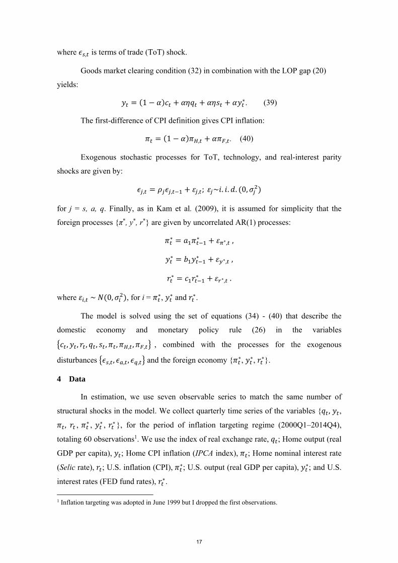
where , is terms of trade (ToT) shock.

Goods market clearing condition (32) in combination with the LOP gap (20)

yields:

1 ∗. (39)

The first-difference of CPI definition gives CPI inflation:

1 , , . (40)

Exogenous stochastic processes for ToT, technology, and real-interest parity

shocks are given by:

, , , ; ~ . . . 0,

for j = s, a, q. Finally, as in Kam et al. (2009), it is assumed for simplicity that the

foreign processes {π*, y*, r*} are given by uncorrelated AR(1) processes:

∗ ∗ ∗, ,

∗ ∗ ∗, ,

∗ ∗ ∗, .

where , ~ 0, , for i = ∗, ∗ and ∗.

The model is solved using the set of equations (34) - (40) that describe the

domestic economy and monetary policy rule (26) in the variables

, , , , , , , , , , combined with the processes for the exogenous

disturbances , , , , , and the foreign economy { ∗, ∗, ∗}.

4 Data

In estimation, we use seven observable series to match the same number of

structural shocks in the model. We collect quarterly time series of the variables { , ,

, , ∗ , ∗ , ∗}, for the period of inflation targeting regime (2000Q1–2014Q4),

totaling 60 observations1. We use the index of real exchange rate, ; Home output (real

GDP per capita), ; Home CPI inflation (IPCA index), ; Home nominal interest rate

(Selic rate), ; U.S. inflation (CPI), ∗; U.S. output (real GDP per capita), ∗; and U.S.

interest rates (FED fund rates), ∗.

                                                            1 Inflation targeting was adopted in June 1999 but I dropped the first observations.

17

Figure 1 presents the quarterly data for the time series over the period 1995-

2014. The data were obtained from the Central Bank of Brazil (http://www.bcb.gov.br)

and Ipea (http://www.ipeadata.gov.br). The data from U.S. were obtained from the

Federal Reserve Bank of St Louis (http://research. stlouisfed.org/fred2).

In the estimation all observables are measured in log percentage deviations from

the steady state which we assumed to be the mean from 1995 to 2014. In the case of the

home output the GDP per capita was constructed dividing the quarterly, seasonally

adjusted, real GDP by the labor force. We use the GDP per capita in log deviations from

a linear trend for the estimation.

Home inflation data correspond to the quarterly log percentage change in the

Brazilian consumer price index (Índice Nacional de Preços ao Consumidor Amplo -

IPCA). Home nominal interest rate corresponds to the 3-month average rates of the

reference interest rate of government bonds (Selic). For the real exchange rate we use

the index of real exchange rate of the Central Bank of Brazil based on a currency basket

of the main trading partners.

18

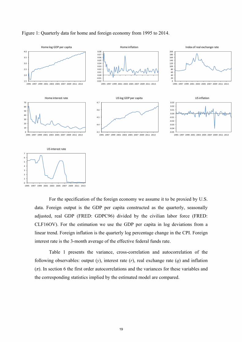
For the specification of the foreign economy we assume it to be proxied by U.S.

data. Foreign output is the GDP per capita constructed as the quarterly, seasonally

adjusted, real GDP (FRED: GDPC96) divided by the civilian labor force (FRED:

CLF16OV). For the estimation we use the GDP per capita in log deviations from a

linear trend. Foreign inflation is the quarterly log percentage change in the CPI. Foreign

interest rate is the 3-month average of the effective federal funds rate.

Table 1 presents the variance, cross-correlation and autocorrelation of the

following observables: output (y), interest rate (r), real exchange rate (q) and inflation

(π). In section 6 the first order autocorrelations and the variances for these variables and

the corresponding statistics implied by the estimated model are compared.

Figure 1: Quarterly data for home and foreign economy from 1995 to 2014.

1.5

2.0

2.5

3.0

3.5

4.0

1995 1997 1999 2001 2003 2005 2007 2009 2011 2013

Home log GDP per capita

‐0.02

‐0.01

0.00

0.01

0.02

0.03

0.04

0.05

0.06

0.07

0.08

1995 1997 1999 2001 2003 2005 2007 2009 2011 2013

Home inflation

0

20

40

60

80

100

120

140

160

180

200

1995 1997 1999 2001 2003 2005 2007 2009 2011 2013

Index of real exchange rate

0

10

20

30

40

50

60

70

1995 1997 1999 2001 2003 2005 2007 2009 2011 2013

Home interest rate

4.3

4.4

4.5

4.6

4.7

1995 1997 1999 2001 2003 2005 2007 2009 2011 2013

US log GDP per capita

‐0.05

‐0.04

‐0.03

‐0.02

‐0.01

0.00

0.01

0.02

0.03

1995 1997 1999 2001 2003 2005 2007 2009 2011 2013

US inflation

0

1

2

3

4

5

6

7

1995 1997 1999 2001 2003 2005 2007 2009 2011 2013

US interest rate

19

5 Estimation methodology

The structural or deep parameters of the model are estimated using Bayesian

methods. First, the second order moments of key observables are compared to those

implied by the estimated model. Then we proceed to the estimation of four versions of

the model. Using Bayesian posterior odds comparisons we test which model is more

probable, all others things been equal. Finally, the comparisons of the DSGE model to

VAR is done using the DSGE-VAR approach of Del Negro et al. (2007).

The set of parameters to be estimated are the central bank preferences

parameters, , , , , the structural parameters, , , , , , , , and

the parameters for exogenous processes , , , , , , , , , , ∗, ∗, ∗ .

The estimation procedure uses the random-walk Metropolis Markov Chain

Monte Carlo (MCMC) method as explained in Del Negro and Schorfheide (2011). The

prior is described by a density function | , where is a specific model and θi

are the parameters of the model. The posterior density of the model parameters θi is

proportional to the likelihood of the sample data Y multiplied by the prior:

| ∝ | | .

The Kalman filter is used to evaluate the likelihood function associated with the

linear state-space model. More specifically, the solution for the log-linearized

equilibrium conditions of the model takes the form of:

Φ Φ ,

where the matrices Φ and Φ are functions of the DSGE model parameters θ, st is a

state vector of model variables and are Gaussian innovations. The model is

augmented by defining a set of measurement equations that relate the elements of st to a

Table 1: Variance, cross-correlation and autocorrelation of output, interest rate, real exchange rate and inflation.

Variance (×10-3)

Cross-correlation Autocorrelation (lag)

y r q π 1 2 3 4

y 0.8592 1 -0.2975 0.0847 -0.2708 0.5475 0.1037 0.2254 0.3943r 0.1235 1 -0.0953 0.3900 0.9373 0.8197 0.7123 0.6455q 6.3832 1 -0.054 0.2467 -0.2006 -0.2248 -0.1148π 0.0928 1 0.4423 -0.0332 -0.0111 0.1684

20

set of observables. Then the Kalman filter is used to estimate the likelihood function

which is combined with the prior distributions for the parameters of the model to form

the posterior density function.

Posterior distribution of the parameters were obtained through the Metropolis-

Hastings sampling algorithm2. We made 100,000 draws from the posterior distribution

using two parallel chains, discarding the first half of the draws to remove any effect of

the initial condition. Then we perform some diagnostic tests to check whether the

MCMC procedure has converged.

After estimation the posterior distribution of competing models we compute the

posterior odds ratio or the Bayes Factor between model i and j:

||

where | is the marginal likelihood of model :

| | .

We use the modified harmonic mean estimator method proposed by Geweke

(1999) to obtain numerical approximations of the marginal likelihood.

The potential misspecification of the DSGE model is assessed using the DSGE-

VAR approach proposed by Del Negro and Schorfheide (2004). They showed how to

combine a DSGE model and a VAR to provide a hybrid model that can be used for

model evaluation, forecasting and monetary policy analysis (Lees et al., 2011).

In the DSGE-VAR approach the priors for the autoregressive matrices of the

VAR are defined by the DSGE model. However, the cross-coefficient restrictions

implied by the DSGE model on the VAR are not strictly imposed. Deviations from

these restrictions are allowed and they are controlled by the hyperparameter λ. If λ = ∞

the restrictions are strictly enforced. If λ = 0 the restrictions are completely ignored in

the estimation of the VAR parameters.

This hyperparameter λ scales the covariance matrix of the prior. If λ is large the

variance is small, and most of the prior mass on the VAR coefficients concentrates near

                                                            2 The estimates were done using Dynare version 4.4.3.

 

21

the DSGE model restrictions. The prior is combined with the likelihood function to

form the posterior distribution of the VAR parameters. For large λ the posterior move

toward the DSGE model restrictions and the less the restrictions are relaxed in the

estimation (Del Negro and Schorfheide, 2011). If λ is small (the variance is big) the

prior on the VAR coefficients is diffuse and the opposite occurs.

The hyperparameter λ is chosen to maximise the marginal data density. High

posterior probabilities for large values of lambda indicate that the model is well

specified. Del Negro and Schorfheide (2006) showed that the shape of the posterior

distribution of λ is robust to the change in the sample and it has an inverse U-shape,

indicating that the fit of the VAR can be improved by relaxing the DSGE model

restrictions.

6 Empirical results

Many empirical studies have assessed which nominal or real frictions are

important to improve the fit of DSGE models. As in Del Negro et al. (2007) we assess

the importance of two particular features of DSGE models: price indexation and habit

formation. They are usually added to models to account for the observed inertia in

inflation and persistence in output. Thus, we run two alternative specifications of the

benchmark model which excludes these two source of frictions. The model without

price indexation is referred as no indexation model and the model without habit

formation as the no habit model. As in Kam et al. (2009) we also test the case where the

central bank is restricted to put no weight on exchange rate variability in its monetary

policy function. This model is referred as the no exchange rate model. In total we have

four different specifications to compare.

Table 2 summarizes the assumptions regarding the prior distribution of each

estimated parameter in the model. We adopt fairly loose priors and their means are

mostly derived from previous studies. We use the beta distribution for all parameters

bounded between 0 and 1. For parameters assumed to be positive, we use the gamma

distribution. Finally, the priors for the standard deviations of the shocks are assumed to

be Inverse Gamma distributed. As in Justiniano and Preston (2010b), the discount factor

β (equal to 0.99) and the share of imports in domestic consumption α (equal to 0.19)

were calibrated. They imply a riskless annual rate of about 4% and the average share of

exports and imports to GDP in Brazil, respectively.

22

6.1. Parameter estimates

Estimated parameters for each model are showed in Table 3. The table reports

the mean and 95% confidence intervals for the benchmark, no indexation, no habit and

no exchange rate models. Univariate convergence diagnostics were performed based on

the ratio of between- and within-chain variances as in Brooks and Gelman (1998). In

general, the tests indicate that the Markov chains have converged to their stationary

distribution.

Analyzing the posterior distributions it is possible to see that a small number of

parameters appear to be weakly identified by the data (Figure 2). It is common in

Bayesian estimation to have some of them with prior similar to posterior distributions

meaning that posterior estimates and log marginal data densities will be sensitive to the

choice of priors (Matheson, 2010).

There are not large variations in the structural parameter estimates across

different model specifications. Nonetheless, the exclusions of habit formation and price

indexation from the model have some effect on the structural parameters as it can be

seen for the inverse elasticities of intertemporal substitution and labor supply. Putting

no weight on exchange rate variability in the monetary policy function of the central

bank affects the other coefficients of the Taylor rule and the persistence parameters of

foreign processes to some degree. For instance, the elasticity of substitution between

home and foreign goods changes from 0.70 to 0.42 in the no exchange model.

The degree of habit persistence (h = 0.79) is similar to the values found in other

studies for Brazil (Palma and Portugal, 2014 and Castro et al., 2011) although it is

higher than the values estimated by Justiniano and Preston (2010b). The (inverse)

intertemporal elasticity of substitution in consumption (σ = 0.96) is relatively lower than

the values reported in the literature implying that the consumption is very sensitive to

real interest rate changes. The inverse elasticity of labor supply is a parameter poorly

identified in DSGE models (Justiniano and Preston, 2010b). In our estimates it is near to

0.5 ϕ 2.05 which is close to the value obtained by Palma and Portugal (2014).

23

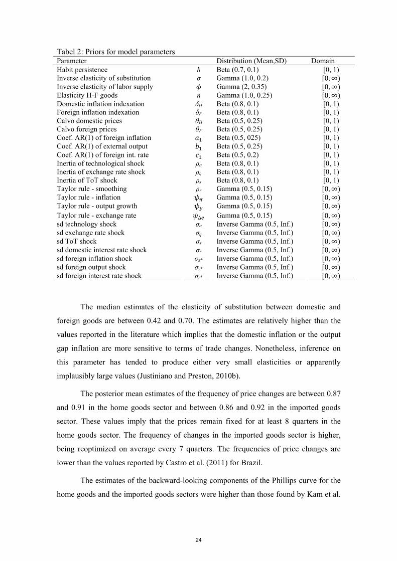
Tabel 2: Priors for model parameters Parameter Distribution (Mean,SD) Domain Habit persistence h Beta (0.7, 0.1) [0, 1) Inverse elasticity of substitution σ Gamma (1.0, 0.2) 0,∞ Inverse elasticity of labor supply Gamma (2, 0.35) 0,∞ Elasticity H-F goods η Gamma (1.0, 0.25) 0,∞ Domestic inflation indexation δH Beta (0.8, 0.1) [0, 1) Foreign inflation indexation δF Beta (0.8, 0.1) [0, 1) Calvo domestic prices θH Beta (0.5, 0.25) [0, 1) Calvo foreign prices θF Beta (0.5, 0.25) [0, 1) Coef. AR(1) of foreign inflation Beta (0.5, 025) [0, 1) Coef. AR(1) of external output Beta (0.5, 0.25) [0, 1) Coef. AR(1) of foreign int. rate Beta (0.5, 0.2) [0, 1) Inertia of technological shock ρa Beta (0.8, 0.1) [0, 1) Inertia of exchange rate shock ρq Beta (0.8, 0.1) [0, 1) Inertia of ToT shock ρs Beta (0.8, 0.1) [0, 1) Taylor rule - smoothing ρr Gamma (0.5, 0.15) 0,∞ Taylor rule - inflation Gamma (0.5, 0.15) 0,∞ Taylor rule - output growth Gamma (0.5, 0.15) 0,∞ Taylor rule - exchange rate ∆ Gamma (0.5, 0.15) 0,∞ sd technology shock σa Inverse Gamma (0.5, Inf.) 0,∞ sd exchange rate shock σq Inverse Gamma (0.5, Inf.) 0,∞ sd ToT shock σs Inverse Gamma (0.5, Inf.) 0,∞ sd domestic interest rate shock σr Inverse Gamma (0.5, Inf.) 0,∞ sd foreign inflation shock σπ* Inverse Gamma (0.5, Inf.) 0,∞ sd foreign output shock σy* Inverse Gamma (0.5, Inf.) 0,∞ sd foreign interest rate shock σr* Inverse Gamma (0.5, Inf.) 0,∞

The median estimates of the elasticity of substitution between domestic and

foreign goods are between 0.42 and 0.70. The estimates are relatively higher than the

values reported in the literature which implies that the domestic inflation or the output

gap inflation are more sensitive to terms of trade changes. Nonetheless, inference on

this parameter has tended to produce either very small elasticities or apparently

implausibly large values (Justiniano and Preston, 2010b).

The posterior mean estimates of the frequency of price changes are between 0.87

and 0.91 in the home goods sector and between 0.86 and 0.92 in the imported goods

sector. These values imply that the prices remain fixed for at least 8 quarters in the

home goods sector. The frequency of changes in the imported goods sector is higher,

being reoptimized on average every 7 quarters. The frequencies of price changes are

lower than the values reported by Castro et al. (2011) for Brazil.

The estimates of the backward-looking components of the Phillips curve for the

home goods and the imported goods sectors were higher than those found by Kam et al.

24

(2009), Justiniano and Preston (2010b) and by Palma and Portugal (2014) for the

Brazilian economy. The exogenous processes for the home economy shocks are in

general persistent, in particular the technology rate shock presents a high degree of

inertia.

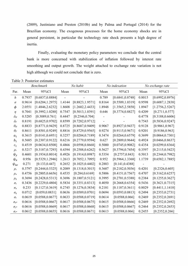
Finally, evaluating the monetary policy parameters we conclude that the central

bank is more concerned with stabilization of inflation followed by interest rate

smoothing and output growth. The weight attached to exchange rate variation is not

high although we could not conclude that is zero.

Table 3: Posterior estimates Benchmark No habit No indexation No exchange rate

Par. Mean 95%CI Mean 95%CI Mean 95%CI Mean 95%CI

h 0.7937 [0.6837,0.8884] - - 0.789 [0.6841,0.8748] 0.8015 [0.6992,0.8976] σ 0.9614 [0.6204,1.2975] 1.4144 [0.8823,1.9571] 0.8164 [0.5509,1.0319] 0.9598 [0.6087,1.2838]

2.0551 [1.4846,2.6232] 1.8608 [1.2602,2.4433] 1.8948 [1.3565,2.5858] 1.8947 [1.2756,2.5267] η 0.7041 [0.3992,1.0288] 0.7547 [0.5013,1.0391] 0.646 [0.3774,0.8827] 0.4209 [0.2711,0.577] δH 0.5285 [0.3089,0.761] 0.4447 [0.2546,0.704] - - 0.4778 [0.3188,0.6606] δF 0.8191 [0.6825,0.9702] 0.8599 [0.7282,0.9712] - - 0.7543 [0.5836,0.9247] θH 0.8833 [0.8771,0.9429] 0.8725 [0.8687,0.9409] 0.9067 [0.8927,0.9437] 0.9128 [0.9061,0.967] θF 0.8611 [0.8501,0.9249] 0.8816 [0.8729,0.9565] 0.9274 [0.9115,0.9671] 0.9201 [0.9186,0.963]

0.3615 [0.0141,0.6951] 0.3257 [0.0204,0.7189] 0.3474 [0.0264,0.6579] 0.3699 [0.0064,0.7301] 0.5685 [0.2307,0.9122] 0.6216 [0.2779,0.9594] 0.627 [0.2809,0.9644] 0.4924 [0.0466,0.8637] 0.4519 [0.0634,0.8508] 0.4866 [0.0598,0.8668] 0.5000 [0.0745,0.9082] 0.4354 [0.0299,0.8364]

ρr 0.5217 [0.3187,0.7293] 0.4394 [0.2588,0.6262] 0.5627 [0.3794,0.7454] 0.3597 [0.2115,0.5423] 0.4601 [0.1934,0.8014] 0.4926 [0.1914,0.8987] 0.5354 [0.2757,0.843] 0.5013 [0.2344,0.7982] 0.956 [0.5329,1.2946] 1.2613 [0.7052,1.7095] 0.952 [0.5964,1.3368] 1.1739 [0.6582,1.7885]

∆ 0.271 [0.133,0.447] 0.2652 [0.1025,0.4402] 0.2883 [0.141,0.4388] - - ρs 0.3797 [0.2444,0.5325] 0.2089 [0.1318,0.3015] 0.3607 [0.2182,0.5036] 0.4201 [0.2326,0.605] ρa 0.4756 [0.2805,0.6656] 0.4535 [0.284,0.6169] 0.5806 [0.4151,0.7567] 0.4707 [0.3162,0.6257] ρq 0.3694 [0.2428,0.5313] 0.3696 [0.1807,0.5121] 0.3995 [0.2701,0.5388] 0.2384 [0.1255,0.3627] σs 0.3436 [0.2229,0.4804] 0.5834 [0.3351,0.8313] 0.4050 [0.2668,0.6354] 0.5436 [0.3621,0.7315] σa 0.233 [0.1127,0.3619] 0.2745 [0.1276,0.3834] 0.2181 [0.1187,0.3611] 0.8029 [0.4411,1.1418] σq 0.0712 [0.059,0.0831] 0.0636 [0.0589,0.0701] 0.0694 [0.0593,0.0813] 0.2494 [0.2353,0.2731] σr 0.0619 [0.0588,0.0677] 0.0633 [0.0588,0.0719] 0.0614 [0.0588,0.066] 0.2469 [0.2352,0.2691] σπ* 0.0616 [0.0588,0.0667] 0.0617 [0.0588,0.0675] 0.0615 [0.0588,0.0666] 0.2469 [0.2352,0.2692] σy* 0.0616 [0.0588,0.0669] 0.0617 [0.0588,0.0668] 0.0615 [0.0588,0.0667] 0.2464 [0.2352,0.2653] σr* 0.0612 [0.0588,0.0655] 0.0616 [0.0588,0.0671] 0.0613 [0.0588,0.066] 0.2455 [0.2352,0.266]

25

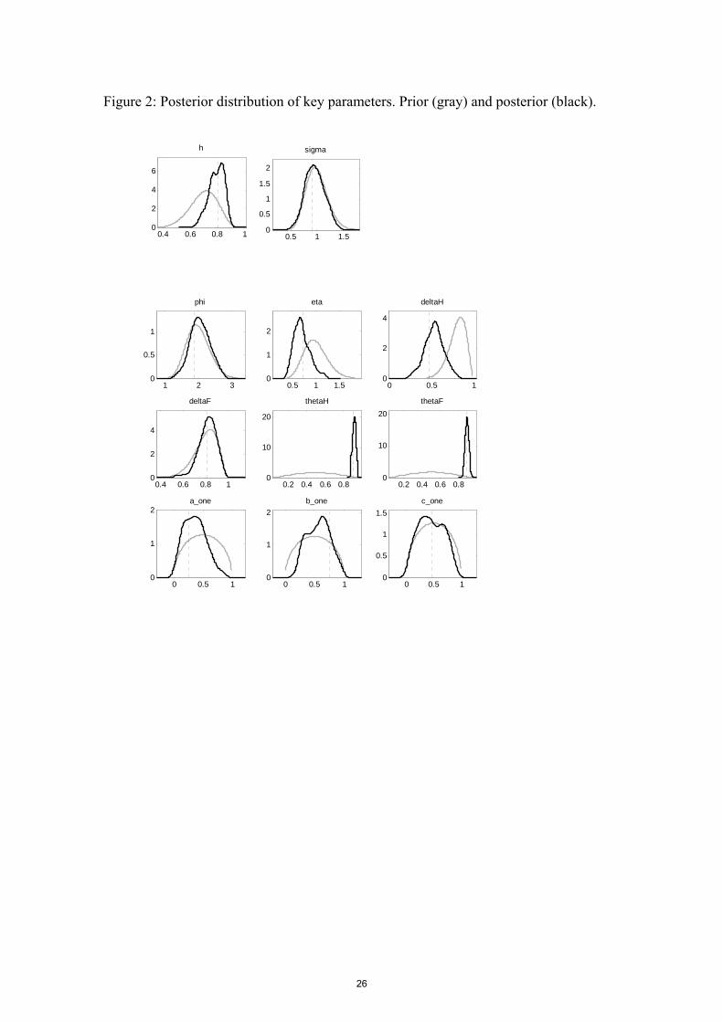
Figure 2: Posterior distribution of key parameters. Prior (gray) and posterior (black).

0.4 0.6 0.8 10

2

4

6

h

0.5 1 1.50

0.5

1

1.5

2

sigma

1 2 30

0.5

1

phi

0.5 1 1.50

1

2

eta

0 0.5 10

2

4

deltaH

0.4 0.6 0.8 10

2

4

deltaF

0.2 0.4 0.6 0.80

10

20

thetaH

0.2 0.4 0.6 0.80

10

20

thetaF

0 0.5 10

1

2a_one

0 0.5 10

1

2

b_one

0 0.5 10

0.5

1

1.5

c_one

26

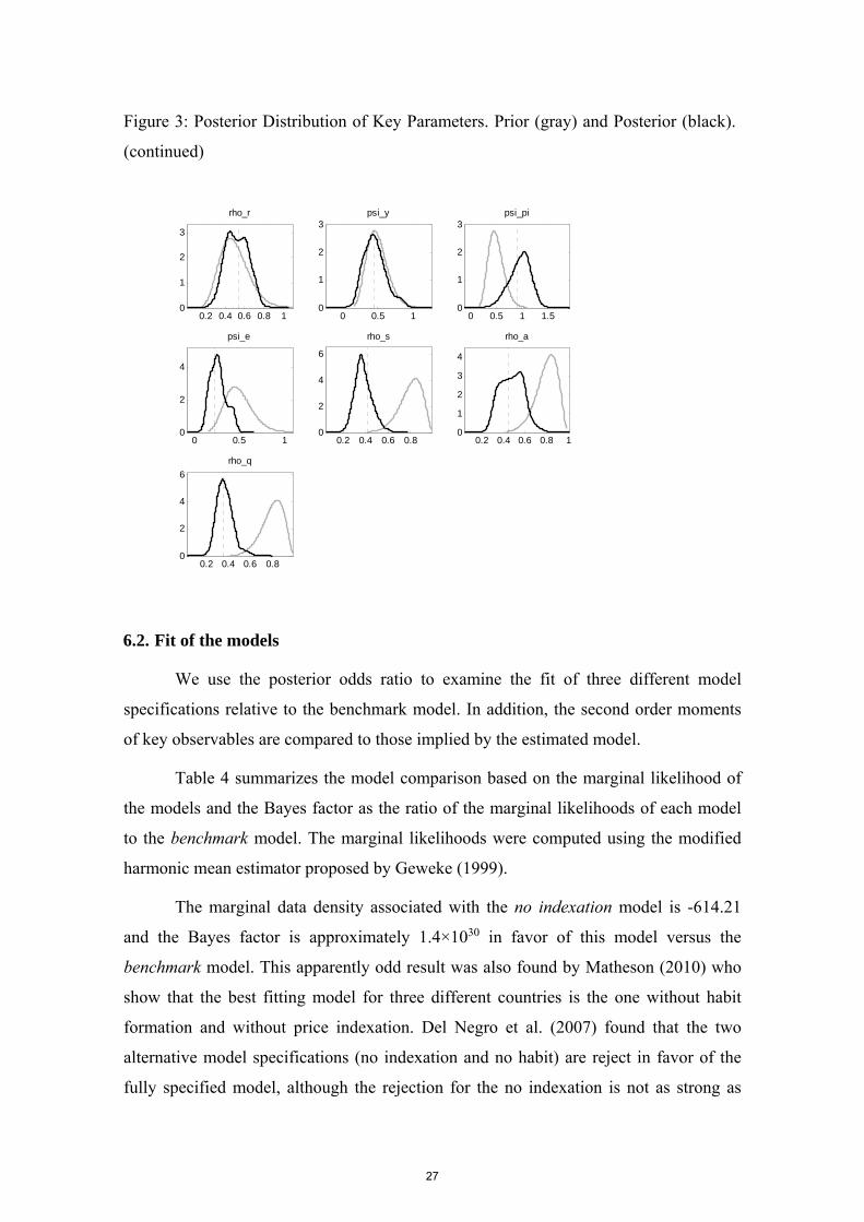
Figure 3: Posterior Distribution of Key Parameters. Prior (gray) and Posterior (black).

(continued)

6.2. Fit of the models

We use the posterior odds ratio to examine the fit of three different model

specifications relative to the benchmark model. In addition, the second order moments

of key observables are compared to those implied by the estimated model.

Table 4 summarizes the model comparison based on the marginal likelihood of

the models and the Bayes factor as the ratio of the marginal likelihoods of each model

to the benchmark model. The marginal likelihoods were computed using the modified

harmonic mean estimator proposed by Geweke (1999).

The marginal data density associated with the no indexation model is -614.21

and the Bayes factor is approximately 1.4×1030 in favor of this model versus the

benchmark model. This apparently odd result was also found by Matheson (2010) who

show that the best fitting model for three different countries is the one without habit

formation and without price indexation. Del Negro et al. (2007) found that the two

alternative model specifications (no indexation and no habit) are reject in favor of the

fully specified model, although the rejection for the no indexation is not as strong as

0.2 0.4 0.6 0.8 10

1

2

3

rho_r

0 0.5 10

1

2

3psi_y

0 0.5 1 1.50

1

2

3psi_pi

0 0.5 10

2

4

psi_e

0.2 0.4 0.6 0.80

2

4

6

rho_s

0.2 0.4 0.6 0.8 10

1

2

3

4

rho_a

0.2 0.4 0.6 0.80

2

4

6

rho_q

27

that for the no habit model. Silveira (2008) using data from Brazil found that both price

indexation and habit formation are important to improve model´s fit though the

evidence is less robust for price indexation.

The marginal data density of the no habit model is -711.04. The Bayes factor of

the model versus the benchmark suggests that the better fit is achieved by the fully

specified model. The same is also true for the no exchange rate model. The marginal

data density is -714.24 and the Bayes factor suggests that the better fit is achieved by

the fully specified model. Hence, we could not conclude that the central bank does not

target exchange rate volatility via its interest rate decisions as in Kam et al. (2009) and

Palma and Portugal (2014).

Table 5 presents the variance and first order autocorrelations of four observables

used to estimate the model: output (y), interest rate (r), real exchange rate (q) and

inflation (π). The comparison exercise provides a measure of absolute fit rather than a

measure of relative fit based on posterior odds ratios. It is possible to see that model

does not match the second order properties of the data so well even though for some

variables the implied variance and autocorrelations are close to their empirical

counterparts. The variance implied by the estimated model for output and real exchange

rate are lower than the variance of the data. For the first order autocorrelations the

model provides a better characterization of the data. The implied autocorrelations are

close to autocorrelations in the data.

Table 4: Log marginal likelihoods and Bayes factors. Specification ln | Bayes Factor Benchmark model -683.62 0 No habit -711.04 -27.41 No indexation -614.21 69.41 No exchange rate -714.24 -30.62

Table 5: Data and implied variances and first order autocorrelations of output, interest rate, real exchange rate and inflation.

Variance (×10-3) First order autocorrelation Data Model Data Model

y 0.8592 0.5192 0.5475 0.5703 r 0.1235 0.2127 0.9373 0.5110 q 6.3832 2.0491 0.2467 0.3400 π 0.0928 0.2473 0.4423 0.5561

28

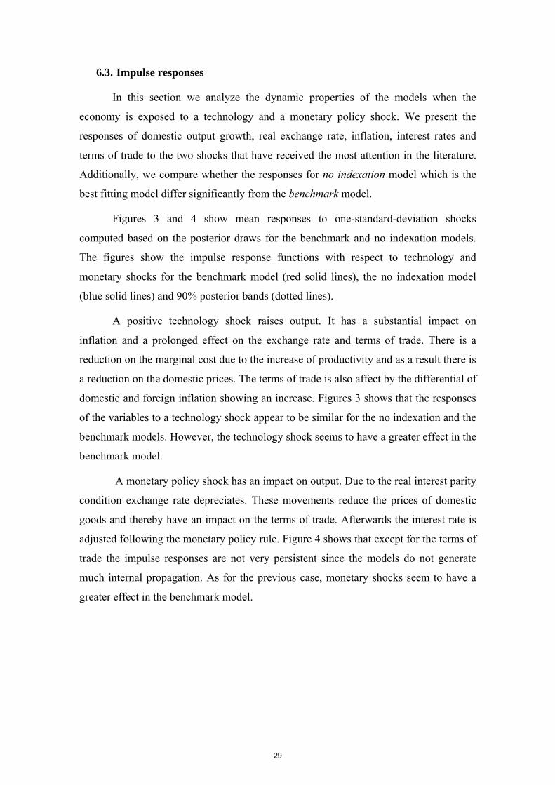
6.3. Impulse responses

In this section we analyze the dynamic properties of the models when the

economy is exposed to a technology and a monetary policy shock. We present the

responses of domestic output growth, real exchange rate, inflation, interest rates and

terms of trade to the two shocks that have received the most attention in the literature.

Additionally, we compare whether the responses for no indexation model which is the

best fitting model differ significantly from the benchmark model.

Figures 3 and 4 show mean responses to one-standard-deviation shocks

computed based on the posterior draws for the benchmark and no indexation models.

The figures show the impulse response functions with respect to technology and

monetary shocks for the benchmark model (red solid lines), the no indexation model

(blue solid lines) and 90% posterior bands (dotted lines).

A positive technology shock raises output. It has a substantial impact on

inflation and a prolonged effect on the exchange rate and terms of trade. There is a

reduction on the marginal cost due to the increase of productivity and as a result there is

a reduction on the domestic prices. The terms of trade is also affect by the differential of

domestic and foreign inflation showing an increase. Figures 3 shows that the responses

of the variables to a technology shock appear to be similar for the no indexation and the

benchmark models. However, the technology shock seems to have a greater effect in the

benchmark model.

A monetary policy shock has an impact on output. Due to the real interest parity

condition exchange rate depreciates. These movements reduce the prices of domestic

goods and thereby have an impact on the terms of trade. Afterwards the interest rate is

adjusted following the monetary policy rule. Figure 4 shows that except for the terms of

trade the impulse responses are not very persistent since the models do not generate

much internal propagation. As for the previous case, monetary shocks seem to have a

greater effect in the benchmark model.

29

Figure 4: Impulse responses to a technology shock for the benchmark model (red solid lines), the

no indexation model (blue solid lines) and 90% posterior bands (dotted lines).

‐1,5E‐03

‐1,0E‐03

‐5,0E‐04

0,0E+00

5,0E‐04

1,0E‐03

0 4 8 12 16

Output

‐1,2E‐02

‐9,0E‐03

‐6,0E‐03

‐3,0E‐03

0,0E+00

3,0E‐03

0 4 8 12 16

Real exchange rate

‐1,2E‐01

‐8,0E‐02

‐4,0E‐02

0,0E+00

4,0E‐02

0 4 8 12 16

Home inflation

‐4,0E‐03

‐2,0E‐03

0,0E+00

2,0E‐03

0 4 8 12 16

Interest rates

‐5,0E‐02

0,0E+00

5,0E‐02

1,0E‐01

1,5E‐01

2,0E‐01

0 4 8 12 16

Terms of trade

30

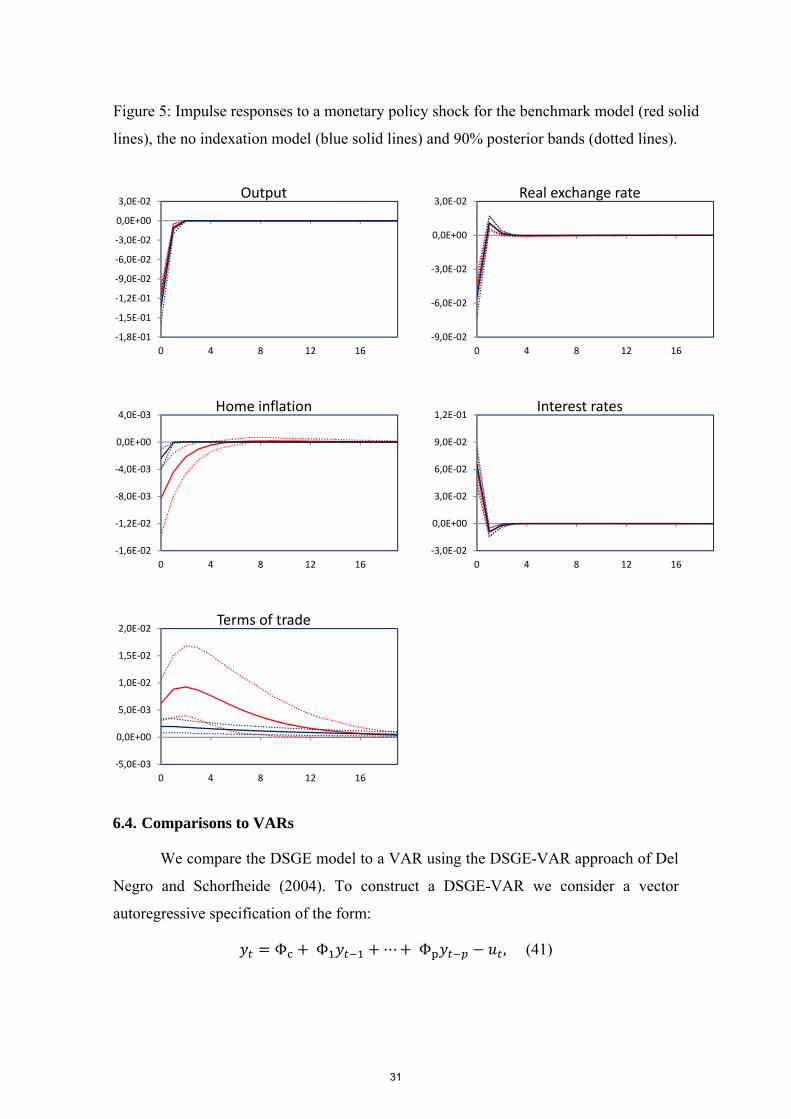
Figure 5: Impulse responses to a monetary policy shock for the benchmark model (red solid

lines), the no indexation model (blue solid lines) and 90% posterior bands (dotted lines).

6.4. Comparisons to VARs

We compare the DSGE model to a VAR using the DSGE-VAR approach of Del

Negro and Schorfheide (2004). To construct a DSGE-VAR we consider a vector

autoregressive specification of the form:

Φ Φ ⋯ Φ , (41)

‐1,8E‐01

‐1,5E‐01

‐1,2E‐01

‐9,0E‐02

‐6,0E‐02

‐3,0E‐02

0,0E+00

3,0E‐02

0 4 8 12 16

Output

‐9,0E‐02

‐6,0E‐02

‐3,0E‐02

0,0E+00

3,0E‐02

0 4 8 12 16

Real exchange rate

‐1,6E‐02

‐1,2E‐02

‐8,0E‐03

‐4,0E‐03

0,0E+00

4,0E‐03

0 4 8 12 16

Home inflation

‐3,0E‐02

0,0E+00

3,0E‐02

6,0E‐02

9,0E‐02

1,2E‐01

0 4 8 12 16

Interest rates

‐5,0E‐03

0,0E+00

5,0E‐03

1,0E‐02

1,5E‐02

2,0E‐02

0 4 8 12 16

Terms of trade

31

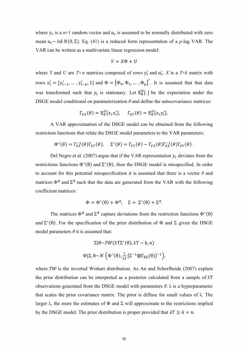
where is a n×1 random vector and is assumed to be normally distributed with zero

mean ~iid 0, Σ . Eq. (41) is a reduced form representation of a p-lag VAR. The

VAR can be written as a multivariate linear regression model:

Φ

where Y and U are T×n matrices composed of rows and . X is a T×k matrix with

rows , … , , 1 and Φ Φ ,Φ ,…, Φ . It is assumed that that data

was transformed such that is stationary. Let . be the expectation under the

DSGE model conditional on parameterization θ and define the autocovariance matrices:

Γ ,Γ .

A VAR approximation of the DSGE model can be obtained from the following

restriction functions that relate the DSGE model parameters to the VAR parameters:

Φ∗ Γ Γ ,Σ∗ Γ Γ Γ Γ .

Del Negro et al. (2007) argue that if the VAR representation deviates from the

restrictions functions Φ∗ θ and Σ∗ θ , then the DSGE model is misspecified. In order

to account for this potential misspecification it is assumed that there is a vector θ and

matrices Φ and Σ such that the data are generated from the VAR with the following

coefficient matrices:

Φ Φ∗ θ Φ ,Σ Σ∗ θ Σ .

The matrices Φ and Σ capture deviations from the restriction functions Φ∗ θ

and Σ∗ θ . For the specification of the prior distribution of Φ and Σ given the DSGE

model parameters θ it is assumed that:

Σ|θ~ λTΣ∗ θ , λT k, n

Φ|Σ, θ~ Φ∗ θ , Σ ⨂Γ θ ,

where is the inverted Wishart distribution. As An and Schorfheide (2007) explain

the prior distribution can be interpreted as a posterior calculated from a sample of λT

observations generated from the DSGE model with parameters θ. λ is a hyperparameter

that scales the prior covariance matrix. The prior is diffuse for small values of λ. The

larger λ, the more the estimates of Φ and Σ will approximate to the restrictions implied

by the DSGE model. The prior distribution is proper provided that .

32

The joint posterior density of VAR and DSGE model parameters can be

factorized as follows:

Φ, Σ, | Φ, Σ| , | .

with the λ subscript indicating the dependence of the posterior on the hyperparameter.

The posterior distribution of Φ and Σ is also of the Inverted Wishart-Normal form (Del

Negro and Schorfheide, 2011):

Σ| , ~ 1 Σ , 1 ,

Φ| , Σ, ~ Φ , Σ⊗ Γ .

Therefore, the larger the weight λ of the prior, the closer the posterior mean of

the VAR parameters is to Φ∗ θ and Σ∗ θ , the values that respect the cross-equation

restrictions of the DSGE model. On the other hand, if λ = (n + k)/T then the posterior

mean is close to the OLS estimate ′ ′ (An and Schorfheide, 2007).

The prior density p(θ) for the DSGE model parameters is determined by the

specification of the prior distributions of the DSGE parameters. The marginal posterior

density of θ can be obtained through the marginal likelihood of | . A derivation is

provided in Del Negro and Schorfheide (2004).

The empirical performance of the DSGE-VAR approach depends on the weight

placed on the DSGE model restrictions. Del Negro et al. (2007) use the marginal data

density as a criterion for the choice of λ:

| .

For computational reasons the hyperparameter λ is restrict to a finite grid Λ. The

normalized can be interpreted as posterior probabilities for λ if it is assigned

equal prior probability to each grid point. Del Negro et al. (2007) define:

∈ Λ | .

If peaks at an intermediate value of λ (between 0.5 and 2, for instance) the

model is not well specified and a comparison between DSGE-VAR( ) and DSGE-

VAR( ∞ ) impulse responses can potentially yield insights about the source of

misspecification (Del Negro et al., 2007).

33

6.5. DSGE-VAR results

We assess the fit of the no indexation, no habit, no exchange and benchmark

models using DSGE-VAR approach. We report the results based on a DSGE-VAR with

four lags. The lag length of the DSGE-VAR is chosen to give a good approximation of

the model3. We show in Table 6 that the VAR approximation error is small. In addition,

it is assumed that λ lies on the finite grid Λ ∈ 0.25, 0.5, 0.75,1, 5, 100 . The log

marginal likelihoods of DSGE-VARs as a function of λ for each model are reported in

Table 6.

The maximum values of the likelihood functions are attained for λ between 0.5

and 0.75. For λ ≥ 1 the values of the marginal likelihoods decrease significantly. The

functions have an inverted U-shape for all models, similar to those found in empirical

applications by Del Negro and Schorfheide (2006). The substantial drop in marginal

likelihood as λ increases is an evidence of the DSGE model misspecification. It reflects

the fact that the fit of the DSGE model is worse than the DSGE-VAR( ) model.

The last row reports the log marginal likelihood of the DSGE model. Comparing

it to the DSGE-VAR(∞), which in our case it is assumed to be λ = 100, it is possible to

check if the VAR can adequately approximate the state-space representation of the

DSGE model. If the VAR approximation of the DSGE model were exact, then the

values of the last two rows would be the same. In our case, they are quite close

suggesting that the VAR approximation error is small.

Table 6: Log marginal likelihoods of DSGE–VAR and DSGE models DSGE-VAR(λ) Benchmark No indexation No habit No exchange λ = 0.25 -670.26 -607.92 -696.44 -706.18 λ = 0.5 -668.43 -605.37 -694.93 -702.16 λ = 0.75 -669.02 -605.43 -695.85 -708.63 λ = 1 -669.97 -605.99 -697.10 -710.22 λ = 5 -678.09 -611.84 -707.03 -715.93 λ = 100 -682.22 -615.36 -711.92 -717.93 DSGE model -683.62 -614.21 -711.04 -714.24

                                                            3 A VAR approximation of the DSGE model is typically not exact because the state-space representation of the linearized DSGE model generates moving average terms. The accuracy of approximation depends on the number of lags p (An and Schorfheide, 2007). 

34

7 Conclusion

In this paper we estimated a DSGE model for a small open economy based on

Kam et al. (2009) using Brazilian economy data for the period of inflation targeting

followed by the Central Bank of Brazil since 1999.

We assessed in a Bayesian framework the empirical fit of four different

specifications of the small open economy model. In particular, we tested the importance

of two particular features of DSGE models: price indexation and habit formation. We

also tested the case where the central bank is restricted to put no weight on exchange

rate variability in its monetary policy function. Finally, the model´s ability to fit

particular second-order characteristics was assessed.

Using posterior odds ratios we found that the best fitting model is the one

without price indexation. Contrary to Palma and Portugal (2014) we could not conclude

that the central bank does not target exchange rate volatility via its interest rate

decisions. The comparison of second order moments showed that as for persistence the

model provides a reasonable characterization of the data. The implied volatilities for

output, interest rate, real exchange rate and inflation are not so close to their empirical

counterparts. The analysis of the impulse response functions have showed that the

dynamics of the variables are quite similar although the shocks have a greater effect in

the benchmark model when compared to the model without price indexation.

Then, we investigated the potential model misspecification implied by invalid

cross-coefficient restrictions on the time series representation generated by the DSGE

model. The model misspecification was tested using the DSGE-VAR approach

developed by Del Negro and Schorfheide (2004) which provides a reliable benchmark

to evaluate the model´s misspecification. The maximum values of the likelihood

functions were attained for λ between 0.5 and 0.75 considering the four competing

model specifications. Therefore, there is an indication of misspecification in this highly

stylized small open economy model.

The reasons for the model misspecification should be investigated in a future

research. The model assumes that shocks across the home and foreign economy are

independent. However, there is ample evidence of comovement in economy activity

across countries. Alternative specifications that assume correlated cross-country shocks

could partially resolve the problem of misspecification (Justiniano and Preston, 2010a).

35

The inclusion of financial frictions into the small open economy setting as in Christiano,

Trabandt and Walentin (2011) could also improve the model´s fit.

36

References

Adalfson, M., Laséen, S., Lindé, J., & Villani, M. (2007). Bayesian estimation of an open economy DSGE model with imcomplete pass-through. Journal of International Economics, 72, pp. 481–511.

Aguiar, M., & Gopinath, G. (2007). Emerging Market Business Cycles: The Cycle Is the Trend. Journal of Political Economy, 115(1), pp. 69-102.

An, S., & Schorfheide, F. (2007). Bayesian analysis of DSGE models. Econometric Reviews, 26(2), pp. 113-172.

Baurle, Gregor & Menz, Tobias (2008). Monetary Policy in a Small Open Economy: a DSGE-VAR approach for Switzerland. Study Center Gerzensee, Working Paper # 08-03

Brooks, S., & Gelman, A. (1998). Alternative Methods for Monitoring Convergence of Iterative Simulations. Journal of Computational and Graphical Studies, 7, pp. 434–55.

Castro, M., Gouvea, S., Minella, A., Santos, R., & Souza-Sobrinho, N. (2011). SAMBA: Stochastic analytical model with a bayesian approach. BCB Working Paper Series, 238, pp. 1-138.

Christiano, L. J., Eichenbaum, M., & Evans, C. (2005). Nominal rigidities and the dynamic effects of a shock to monetary policy. Journal of Political Economy, 113, pp. 1-45.

Christiano, L. J., Trabandt, M., & Walentin, K. (2011). Introducing financial frictions and unemployment into a small open economy model. Journal of Economic Dynamics and Control, 35(12), 1999–2041.

Del Negro, M., & Schorfheide, F. (2004). Priors from general equilibrium models for VARs. International Economic Review, 45, pp. 643-673.

Del Negro, M., & Schorfheide, F. (2006). How Good Is What You've Got? DSGE-VAR as a Toolkit for Evaluating DSGE Models. Federal Reserve Bank of Atlanta Economic Review, 91(2), pp. 21-37.

Del Negro, M., & Schorfheide, F. (2008). Inflation Dynamics in a Small Open-Economy Model under Inflation Targeting: Some Evidence from Chile. Federal Reserve Bank of New York Staff Reports, no. 329, pp. 1-49.

Del Negro, M., & Schorfheide, F. (2011). Bayesian Macroeconometrics. The Oxford Handbook of Bayesian Econometrics, pp. 293-389.

Del Negro, M., Schorfheide, F., Smets, F., & Wouters, R. (2007). On the Fit of New Keynesian Models. Journal of Business and Economic Statistics, 25(2), pp. 123-143.

Devereux, M., Lane, P., & Xu, J. (2006). Exchange rates and monetary policy in emerging market. Economic Journal, 116(511), pp. 478-506.

Galí, J., & Monacelli, T. (2005). Monetary Policy and Exchange Rate Volatility in a Small Open Economy. Review of Economic Studies(72), pp. 707–734.

García-Cicco, J., Pancrazi, R., & Uribe, M. (2010). Real Business Cycles in Emerging Countries? American Economic Review, 100, pp. 2510–2531.

Geweke, J. (1999). Using simulation methods for Bayesian econometric models. Econometric Reviews, 18, pp. 1-126.

37

Gupta, Rangan & Steinbach, Rudi (2013). Forecasting key macroeconomic variables of the South Africa Economy: a small open economy New Keynesian DSGE-VAR model. Economic Modelling, 33(1), p. 19-33.

Hove, S., Mama, A. T., & Tchana, F. T. (2015). Terms of Trade Shocks and Inflation Targeting in Emerging Market Economies. South African Journal of Economics.

Justiniano, A., & Preston, B. (2010a). Can structural small open-economy models account for the influence of foreign disturbances? Journal of International Economics, 81, pp. 61-74.

Justiniano, A., & Preston, B. (2010b). Monetary policy and uncertainty in an empirical small open-economy model. Journal of Applied Econometrics, 25, pp. 93-128.

Kam, T., Lees, K., & Liu, P. (2009). Uncovering the Hit List for Small Inflation Targeters: A Bayesian Structural Analysis. Journal of Money, Credit and Banking, 41(4).

Kollmann, R. (2002). Monetary policy rules in the open economy: effects on welfare and business cycles. Journal of Monetary Economics, 49, pp. 989-1015.

Lees, K., Matheson, T., & Smith, C. (2011). Open economy forecasting with a DSGE-VAR: Head to head with the RBNZ published forecasts. International Journal of Forecasting, 27, pp. 512-528.

Lubik, T., & Schorfheide, F. (2007). Do Central Banks Respond to Exchange Rate Movements? A Structural Investigation. Journal of Monetary Economics, 54, pp. 1069–87.

Marcelino, Massimiliano & Rychalovska, Yuliya (2014). Forecasting with a DSGE Model of a Small Open Economy within the Monetary Union. Journal of Forecasting, 33(5), p. 315-338.

Matheson, T. (2010). Assessing the fit of small open economy DSGEs. Journal of Macroeconomics, 32, pp. 906-920.

Monacelli, T. (2005). Monetary policy in a low pass-through environment. Journal of Money, Credit and Banking, pp. 1047-1066.

Palma, A., & Portugal, M. (2014). Preferences of the Central Bank of Brazil under the inflation targeting regime: estimation using a DSGE model for a small open economy. Journal of Policy Modeling, 36, pp. 824–839.

Schmitt-Grohé, S., & Uribe, M. (2001). Stabilization Policy and the Costs of Dollarization. Journal of Money, Credit and Banking, 33, pp. 482-509.

Silveira, M. (2008). Using a bayesian approach to estimate and compare new keynesian DSGE models for the Brazilian economy. Revista Brasileira de Economia, 62(3), pp. 333–357.

Smets, F., & Wouters, R. (2002). Openness, imperfect exchange rate pass-through and monetary policy. Journal of Monetary Economics, 49, pp. 913-940.

Smets, F., & Wouters, R. (2003). An estimated dynamic stochastic general equilibrium model of the euro area. Journal of the European Economic Association, 1(5), pp. 1123-1175.

38

Uribe, M., & Yue, V. (2006). Country spreads and emerging countries: Who drives whom? Journal of International Economics, 69(1), pp. 6-36.

39