FEM Analysis in Sensor Development – Siemens VDO Sas M., Bizon L.

Siemens VDO Automotive Czech Republic

Abstract

At the development of sensors with electrical output in automotive applications are different optimizations taken into the consideration like geometry shape, placement of the sensor, ambient condition, chemical interaction, used material proposition, electrical components and their influence, accuracy, response and durability. These parameters and factors are designed, evaluated and simulated by proper CAD1 tool and a series of real tests and measurements, but between the designing and real testing the FEM2 analysis can take a big portion of work before building a real part and test it in real condition. This step could be a really time and money saving in case of developing a competitive temperature, level, speed or pressure sensor.

Keywords: FEM Analysis, Thermal transient analysis, Thermodynamics, CFD3, Eigen frequencies, Response time, Electromagnetism, NTC4 thermistor.

1 Introduction

The article is oriented at the achieved and future application in domain of FEM analysis of temperature and level sensors in Siemens VDO, which is a worldwide supplier of quality products for automotive industry. The division of sensors has their application mainly in Powertrain systems like engines, pumps, coolants, tanks etc.

Simulations are made in domains of physics like thermodynamics, flow dynamics, structure mechanics, and electromagnetisms with 2D and 3D parts and assemblies.

2 Results

Mathematical model for heat transfer analysis by conduction is the heat equation where T is temperature, ρ is the density, C is the heat capacity (Cp, CV), k is the thermal conductivity, Q is a heat source or sink.

QTkt

TC =∇−∇+

∂∂

).(ρ (1)

To add the convection through a fluid in Eq. (1)

QCTuTkt

TC =+∇−∇+

∂∂

).( ρρ (2)

where the expression in brackets represent the heat flux vector q [1].

Each model and applications are described in following subsections.

1 CAD – Computed Aided Design 2 FEM – Finite Element Method numerical analysis 3 CFD – Computational Flow Dynamics 4 NTC – Negative Temperature Coefficient resistant temperature sensing element

2.1 Thermal Analysis

Thermodynamics which is mainly applied in temperature sensor analysis contains studies of stationary and mainly transient analysis with applied conduction, convection and radiation. These analyses are made in purpose of achieving an optimization of response time curve in area of NTC thermistor – sensing element which is changing its electrical resistance with changing temperature. The response time, like a main indicator, is the time that the temperature sensor needs to change 63.2 % (or 90 %) of the temperature difference between initial and final temperature. This indicator is mainly influenced by design of the sensor, used materials and additionally by ambient conditions like flow velocity and type of measured medium.

Resistant temperature sensors can be defined like a static element of first order without delay td which can be described with the following firs order differential equations with constant coefficients of transitional function [2]

uyaya =+ .. 0'

1 (3)

ukyytk ... ' = (4)

k=1/a0 (5)

)1.( / ktteky −−= (6)

Equations are giving a picture about the behavior of the temperature sensors in transitional state as a function of time (Figure 1.) in time interval of output quantity y as a reaction on the action of the step change of input quantity u until the stabilization in the course of time constant tk.

Figure 1. Transitional function of resistant temp. sensors.

Influence of temperature is simulated also for level sensor and the typical ranges of use for both are from -40ºC to +150ºC. The calculation of response time is than confirmed by series of real measurements which are then supplemented by real thermal cyclic shocks tests for revealing the overall endurance of the sensors.

Figure 2. Post-processed data of a 3D model temp. sensor transient analysis.

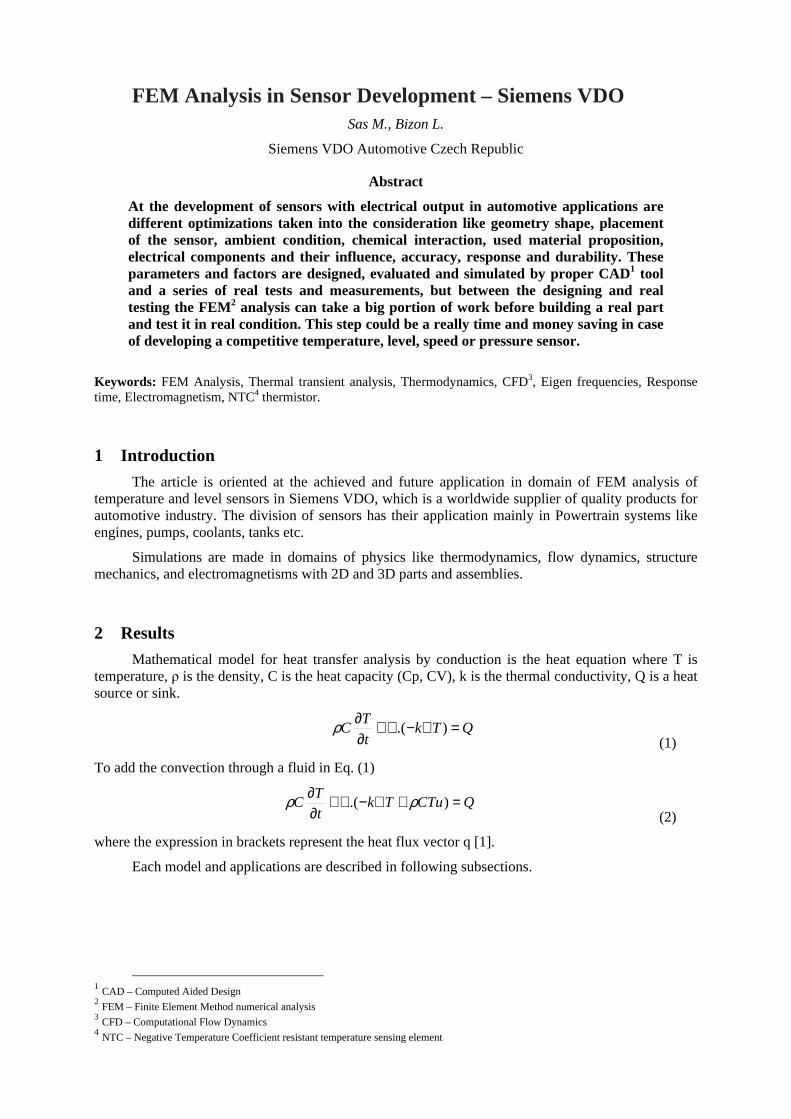
2.2 Structure Analysis

In structure mechanics domain mostly a frequencies analysis is taken into the account, like eigenfrequencies and frequency response analysis for the maximum of displacement for a specified range of frequencies of the sensor assembly.

Figure 3. 3D model of a level sensor in frequency response analysis - maximum displacement amplitude in x direction.

Then also a thermal stresses, strains and displacements are calculated because of better designing of parts and used materials. Force and torques loads analysis are realized more rarely in Comsol, although these kind of analysis are performed directly in CAD designing software and in case of more importance are compared with results from Comsol. These kinds of analysis are also confirmed by series of realized tests according to demands and specifications for the sensors.

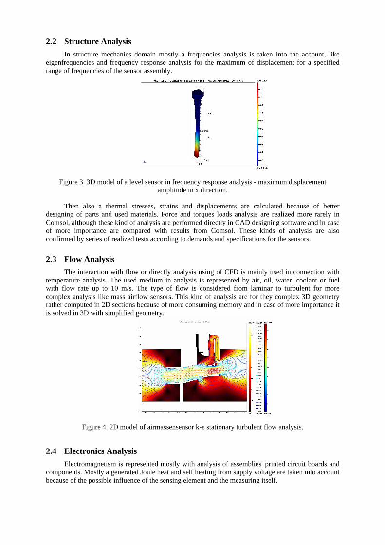
2.3 Flow Analysis

The interaction with flow or directly analysis using of CFD is mainly used in connection with temperature analysis. The used medium in analysis is represented by air, oil, water, coolant or fuel with flow rate up to 10 m/s. The type of flow is considered from laminar to turbulent for more complex analysis like mass airflow sensors. This kind of analysis are for they complex 3D geometry rather computed in 2D sections because of more consuming memory and in case of more importance it is solved in 3D with simplified geometry.

Figure 4. 2D model of airmassensensor k-ε stationary turbulent flow analysis.

2.4 Electronics Analysis

Electromagnetism is represented mostly with analysis of assemblies' printed circuit boards and components. Mostly a generated Joule heat and self heating from supply voltage are taken into account because of the possible influence of the sensing element and the measuring itself.

Figure 5. 3D model of PCB – thermal stationary analysis (self heating included).

3 Meshing Methods

Meshes are created mostly with tetrahedral structure for 2D and 3D tasks. For an assembly different kind of parameters of meshing is used for each part (subdomain).

The typical number of degrees of freedom is about 250k and number of elements about 180k.

Figure 6. Pre-processing the model for calculation – tetrahedral mesh.

Only a connected mesh is considered so no pairs or imprints are created for further processing for achieving the best results.

4 Numerical Models

Initial and boundary conditions are set as close as possible to the real conditions of the real physical test or measurement (response time, vibrations, flow interaction). In thermal analysis for transient cases the initial condition is initial temperature and the boundary conditions are heat flux at the all outside surfaces with constant heat transfer coeff. and external temperature. No radiation is applied.

Figure 7. Example of a boundary conditions: Heat flux: Inward heat flux: 0[W/m2]; Heat transfer coeff.: 150[W/m2.K]; External temp.:90[ºC] – applied on cup of the sensor.

Used materials are mostly a polyamides, silicon pastes, stainless steel, CuSn, copper, MgO, etc.

Figure 8. Constraints defined as a described acceleration. Rest of the model is without any constraints and loads.

Vibrations and eigenfrequencies are defined according the real constraints conditions and applied loads. Different designs, shapes and conditions (different temperature = different Young's modulus) are considered to improve the range of the frequencies and so the robustness of the design.

5 FEM Analysis Results

Post-processing data are giving accurate results in sense of comparing different cases or designs – relative results, and also the absolute results are close to the reality in about 88% to 95%. Purpose of the analysis is to have more designs to compare the differences and choose the best solution.

Figure 9. Response time for 63.2% of temp. step change which represents temperature of 65.5 ºC is 13.2s

Different type of visual results are useful, like total heat flux, temperature gradient etc. to see the influence of geometric shape and material.

Ax = 80 [m/s2]

Ay,Az = 0 [m/s2]

Figure 10. Total heat flux in direction from the heated cup (90ºC) through the sensor.

Then the results like response time – point plot are used for optimizing the design and materials. For example two different designs of cup for temperature sensor (5mm difference in length) was designed - long and short one with following analysis results in resp. time. This difference of 5mm in length makes indirect proportion to the resp. time in difference of 1.5s

Comparing of 2 designs

25

35

45

55

65

75

85

95

-5 5 15 25 35 45 55 65 75

Time [s]

Tep

erat

ure

[C]

Temp.long design [C]

Temp.short version [C]

Figure 11. Response time for 63.2% of temp. step change from 25ºC to 90ºC which represents temperature of 65.5ºC. Difference 5mm in length makes indirect proportion to the resp. time

difference of 1.5s.

Then a differences in used thermo paste was calculated for shorter design (thermal conductivity k=1.7[W/m.K] and k=2.0[W/m.K]) and its influence and relation on resp. time is also indirect proportional in difference of 0.9s.

Comparing different thermopaste for one design

25

35

45

55

65

75

85

95

-5 5 15 25 35 45 55 65 75

Time [s]

Tem

per

atu

re [

C]

Temperature[C] (k=1.7[W/m.K])

Temperature[C] (k=2.0[W/m.K])

Figure 12. Differences in used thermo paste was calculated for shorter design makes also indirect proportional in difference of 0.9s.

τ63.2=11.7s – for long design

τ63.2=13.2s – for short design

τ63.2=13.2s – for k=1.7[W/m.K]

τ63.2=12.3s – for k=2.0[W/m.K]

For a structure analysis a calculations of eigenfrequencies is mainly considered with boundary conditions set to constraints according to mounting position and fixation. No load and damping need to be applied.

Figure 13. First 4 eigenfrequencies for temp. sensor.

Than follows maximal displacement amplitude near the eigenfrequencies range and in certain direction with defined constraint of acceleration, e.g. 8g is applied. Also max. stress are in interest and thermal dilatation. Where also a point plot values is created to see the max. displacement.

Figure 13. For temperature -40ºC calculated maximum displacement amplitude in x direction with max. von Mises stress 8.9[MPa] and max. displacement amplitude in x direction is 0.123 [mm] @ 395

[Hz].

For a flow analysis an example of airmassensensor was solved in 2D k-ε stationary turbulent flow analysis focused at the place of the sensing element.

Figure 15. Velocity field in area of sensing element (max. 3 m/s) with streamlines of the flow.

Sections for velocity and pressure curves are made in vertical and horizontal directions to see the distribution of velocity and pressure in numbers.

Figure 16. Velocity field and pressure in vertical line section in area of the sensing element

Then according to the application of intake air temperature sensors in a turbulent flow of a tube with inserted sensor is simulated in 3D k-ε stationary turbulent flow analysis.

Figure 17. Velocity field (max. 25.7 m/s) with streamlines of the flow and velocity field (max. 25.7 m/s).

And also with section plots of interesting parameters in specified directions.

Figure 19. Velocity field and pressure in vertical line section through the center axis of the sensor

6 Experimental Results

Mostly it is possible to compare the calculated results to a real tests measurement or vice versa to confirm the real data from previous experiences with a numerical model as it is shown at following example of a temperature sensor.

Figure 20. X-ray photo of real sample and measured response time of real sample.

Response time for 63.2% of temp. step change (at temp. of 65.5ºC) is 12.3s and was measured in silicon oil with heat transfer coeff. set to 150[W/m2.K].

The calculated results can be seen in previous section no. 5. to compare the results:

Calculated: τ63.2=13.2s

Measured: τ63.2=12.3s

which represents difference of 0.9s and accuracy of solution to 92.7%.

7 Conclusions

The interactions of different physical domains are applied in solutions of different sensors for different applications according to customer demands and latest technology and material trends in automotive industry.

Each task is solved with maximum approximation to the real conditions, geometry and material properties to confirm real test results. For the future analysis it is planed to make an optimization of key parameters in connection with Matlab.

References [1] John H. Lienhard, A Heat Transfer Textbook, 193-330. Phlogiston Press, Cambridge

Massachusetts (2006) [2] Kříž, R., Vávra P., Strojárenská príručka 2. svazek, Praha: Scientica s.r.o., 1993. 34-152 s. ISBN-

0-112-03247-3

Sas Martin Contact information: Siemens VDO [Siemens Automotive Systems]; Kopanska 1713; 744 01 Frenstat p. R.; Czech Republic E-Mail: martin.sas@siemens.com; Internet: http://www.siemensvdo.com Bizon Lukas Contact information: Siemens VDO [Siemens Automotive Systems]; Kopanska 1713; 744 01 Frenstat p. R.; Czech Republic E-Mail: lukas.bizon@siemens.com; Internet: http://www.siemensvdo.com

Measured resp. time for short design

0.0

10.0

20.0

30.0

40.0

50.0

60.0

70.0

80.0

90.0

0 5 10 15 20 25 30 35 40 45 50 55 60 65 70 75 80 85 90 95 Time (s)

Tem

erat

ure

(C

)

0.0

0.5

1.0

1.5

2.0

2.5

3.0

3.5

4.0

Vo

ltag

e (V

)

T (C)U(V)

12.3s