FEEDFORWARD NETWORKS: ADAPTATION, …mrasmuss/preprints/DynamIC_2018_4.pdf · FEEDFORWARD NETWORKS:...

FEEDFORWARD NETWORKS: ADAPTATION,FEEDBACK, AND SYNCHRONY

MANUELA AGUIAR, ANA DIAS, AND MICHAEL FIELD

Abstract. In this article we investigate the effect on synchronyof adding feedback loops and adaptation to a large class of feedfor-ward networks. We obtain relatively complete results on synchronyfor identical cell networks with additive input structure and feed-back from the final to the initial layer of the network. These re-sults extend previous work on synchrony in feedforward networksby Aguiar, Dias and Ferreira [1]. We also describe additive andmultiplicative adaptation schemes that are synchrony preservingand briefly comment on dynamical protocols for running the feed-forward network that relate to unsupervised learning in neural netsand neuroscience.

Contents

1. Introduction 21.1. Background on feedforward networks 21.2. Objectives and Motivation 51.3. Main results and outline of paper 92. A class of networks with additive input structure 102.1. Dynamical networks with additive input structure 102.2. Synchrony subspaces 112.3. Network compatibility 133. Adaptation and Weight Dynamics 174. Layered structure and feed forward networks 204.1. Notation and assumptions 214.2. Feedback structures on an (A)FFNN 214.3. Synchrony for FFNNs with feedback structure. 234.4. Synchrony for AFFNNs with feedback structure 284.5. {2, . . . , ℓ− 1}-feedback structures on (A)FFNNs 345. Concluding remarks 34References 35

Date: March 14, 2018.1

2 MANUELA AGUIAR, ANA DIAS, AND MICHAEL FIELD

1. Introduction

This paper is about the effect on synchrony of adding feedback loopsand adaptation to feedforward networks and is part of a study of dy-namics and bifurcation in feedforward and functional networks devel-oping out of prior work of Aguiar et al. [1] and Bick et al. [4, 5].

1.1. Background on feedforward networks. Dynamicists typicallyregard a network of dynamical systems as modelled by a graph withvertices or nodes representing individual dynamical systems, and edges(usually directed) codifying interactions between nodes. Usually, evolu-tion is governed by a system of ordinary differential equations (ODEs)with each variable tied to a node of the graph. Examples include theubiquitous Kuramoto phase oscillator network, which models weak cou-pling between nonlinear oscillators [24, 20], and coupled cell systemsas formalised by Golubitsky, Stewart et al. [37, 16, 15].Feedforward networks play a well-known and important role in net-

work theory and appear in many applications ranging from synchro-nization in feed-forward neuronal networks [14, 34], to the modelling oflearning and computation—data processing (see below). Yet feedfor-ward networks often do not fit smoothly into the dynamicists lexicon fornetworks. Feedforward networks, such as artificial neural nets (ANNs)and network models for visualization and learning in the brain, usuallyprocess input data sequentially and not synchronously as is the case ina dynamical network. More precisely, a feedforward network is dividedinto layers—the (hidden) layers of an ANN—and processing proceedslayer-by-layer rather than simultaneously across all layers as happenswith networks modelled by systems of differential equations. The wayin which data is processed—synchronously or sequentially—can have amajor impact on both dynamics and output (see Example 1.2 below).An additional feature of many feedforward networks is that they havea function, represented by going from the input layer to the outputlayer. Optimization of network function typically requires the networkto be adaptive.

Example 1.1 (Artificial Neural Nets & Supervised Learning). Theinterest in ANNs lies in their potential for approximating or represent-ing highly complex and essentially unknown functions. For example,a map from a large set of facial images to a set of individuals withthose facial images (facial recognition) or from a large set of drawn orprinted characters to the actual characters (handwriting recognition).An approximation to the required function is obtained by a process oftraining and adaptation. No attempt is made to derive an “analytic”

FEEDFORWARD NETWORKS 3

form for the function. We sketch only the simplest model and refer thereader to the extensive literature for more details, greater generalityand related methods [7, 18, 19, 35, 17].

Hidden layers

Out

put l

ayer

Inpu

t lay

er(b)

a

b

c

z

y

x

Sigmoid Neuron

(a)

Perceptron

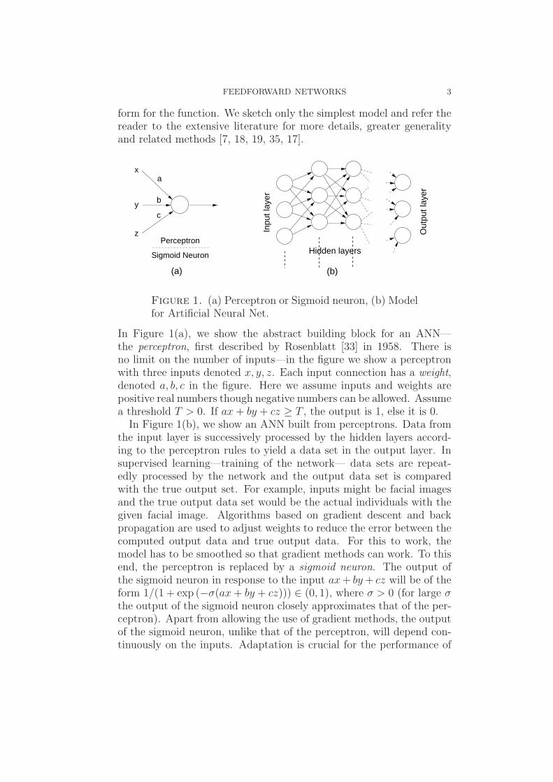
Figure 1. (a) Perceptron or Sigmoid neuron, (b) Modelfor Artificial Neural Net.

In Figure 1(a), we show the abstract building block for an ANN—the perceptron, first described by Rosenblatt [33] in 1958. There isno limit on the number of inputs—in the figure we show a perceptronwith three inputs denoted x, y, z. Each input connection has a weight,denoted a, b, c in the figure. Here we assume inputs and weights arepositive real numbers though negative numbers can be allowed. Assumea threshold T > 0. If ax+ by + cz ≥ T , the output is 1, else it is 0.In Figure 1(b), we show an ANN built from perceptrons. Data from

the input layer is successively processed by the hidden layers accord-ing to the perceptron rules to yield a data set in the output layer. Insupervised learning—training of the network— data sets are repeat-edly processed by the network and the output data set is comparedwith the true output set. For example, inputs might be facial imagesand the true output data set would be the actual individuals with thegiven facial image. Algorithms based on gradient descent and backpropagation are used to adjust weights to reduce the error between thecomputed output data and true output data. For this to work, themodel has to be smoothed so that gradient methods can work. To thisend, the perceptron is replaced by a sigmoid neuron. The output ofthe sigmoid neuron in response to the input ax+ by+ cz will be of theform 1/(1 + exp (−σ(ax+ by + cz))) ∈ (0, 1), where σ > 0 (for large σthe output of the sigmoid neuron closely approximates that of the per-ceptron). Apart from allowing the use of gradient methods, the outputof the sigmoid neuron, unlike that of the perceptron, will depend con-tinuously on the inputs. Adaptation is crucial for the performance of


artificial neural networks: Minsky and Papertin showed in their 1969book [30] that, without adaptation, ANNs based on the perceptroncould not perform some basic pattern recognition operations.From a dynamical point of view, an ANN can be regarded as a com-

posite of maps—one for each layer—followed by a map acting on weightspace. Note that the processing is layer-by-layer and not synchronous.In particular, an artificial neural net is not modelled by a discrete dy-namical system—at least in the conventional sense.The inspiration for artificial neural nets comes from neuroscience

and learning. In particular, the perceptron is a model for a spikingneuron. The adaptation, although inspired by ideas from neuroscienceand Hebbian learning, is global in character and does not have anobvious counterpart in neuroscience.

There does not seem to be a natural or productive way to replace thenodes in an ANN with continuous dynamical systems—at least withinthe framework of supervised learning. Indeed, the supervised learningmodel attempts to construct a good approximation to a function thatacts on data sets. This is already a hard problem and it is not clearwhy one would want to develop the framework to handle data setsparametrised by time1. However, matters change when one considersunsupervised learning. In this case there are models from neuroscienceinvolving synaptic plasticity, such as Spike-Timing Dependent Plastic-ity (STDP), which involve dynamics and asynchronous or sequentialcomputation. In the case of STDP, learning and adaptation are con-trolled by relative timings of spike firing (we refer to [13, 31, 8] formore details, examples and references and note that adaptive rules fora weight typically depend only on states of neurons at either end of theconnection—axon). It has been observed that adaptive models usingSTDP are capable of pattern recognition in noisy data streams (forexample, [27, 28, 29]).As a possible application of this viewpoint, one can envisage data

processing of a continuous data stream by an adaptive feedforwardnetwork comprised of layers consisting of continuous dynamical units.Here the output would reflect dynamical structure in the data stream—for example, periodicity or quantifiable chaotic behaviour. The pro-cessing could be viewed as a dynamic filter and the approach can becontrasted with reconstruction techniques based on the Takens embed-ding theorem.

1In dynamical systems theory there are methods based on the Takens embeddingtheorem [38] that allow reconstruction of complex dynamical systems from timeseries data. However, these techniques seem not to be useful in data processing.


1.2. Objectives and Motivation. Dynamical feedforward networksmay be viewed as relatively primitive networks, at least from an evolu-tionary viewpoint. It is natural to consider how the network structurecan evolve so as to optimise network function (for example, patternrecognition). One way of doing this is to consider the effect of addingfeedback loops to the network. Perhaps surprisingly, the addition offeedback to a feedforward network can lead to dramatic bifurcation inthe synchrony structure of the network. Specifically, the addition offeedback loops can enrich the synchrony structure and result in, for ex-ample, periodic synchrony patterns that do not occur for feedforwardnetworks without feedback. The existence of a rich synchrony structureis an indicator for the potential of the network in learning applications(for example, pattern recognition). In this case, rather than internalsynchronization between nodes, the objective is to synchronize somenodes with components of the incoming data stream2. As an illustra-tion of this phenomenon, we cite the mechanism of STDP which canlead to synchronization of a small subset of nodes with a repeatingcomponent in a noisy data stream [27] or, via similar mechanisms, leadto direction location [13]. Our objective here is more modest and di-rected towards gaining a better understanding of how the synchronystructure of a feedforward network changes when feedback is added tothe network. The determination of the synchrony structure of the net-work needs to be done in a way that is compatible with adaptation.That is, aside from describing how adaptation should work, there is aneed to identify types of adaptation that will not destroy the synchronystructure of the network.Although the main focus of this article is on synchrony and the dy-

namics of adaptation, it is helpful to say a little more about some ofthe issues involving dynamics and bifurcation. First, it is well-knownthat the addition of feedback loops may have deleterious effects on thedynamics and functionality of a network—for example, in transportnetworks containing loops overlapping other routes (for example, theCircle line in the London underground system [32]) or the Bullwhipeffect in stock-inventory control systems [25]. It is natural to describebifurcation of dynamics that can occur with the addition of feedbackloops to a feedforward network. In particular, from an evolutionarypoint of view, dynamic bifurcation is significant in the context of op-timising network function (see also the discussions in [5, §6], [4, §1.6]).

2For effective and efficient implementation of this approach, it is expedient tointroduce some intra-layer inhibitory structure (for example [28, 26]).


There is also the question of whether the network processes data syn-chronously or asynchronously (for example, see [5] and the examplefollowing) and the effect this may have on the computational effective-ness and dynamics of running a feedforward dynamical network. Ina companion paper [2] we give more detailed results and examples ondynamics. For now we give some numerics that illustrate the rich dy-namics that can occur in feedforward networks with feedback and howthe way the network is run can have unexpected and dramatic effectson the output.

Example 1.2 (A feedforward network of theta neurons). The dynam-ics of a theta neuron [11] are given by

θ′ = (1− cos(2πθ)) + η(1 + cos(2πθ)), θ ∈ R/Z.

If η > 0 (excitable case), dynamics is periodic; if η < 0, there are twoequilibria, one of which is attracting.Following Chandra et al. [9], we consider a network N of 50 theta

neurons with dynamics of node i, 1 ≤ i ≤ 50, given by

θ′i = (1− cos(2πθi)) + (1 + cos(2πθi))(ηi + Ii),(1.1)

Ii = si∑

j∈50

wijP (θj),(1.2)

where P (θ) = 26(6!)2

12!(1 − cos(2πθ))6 is a ‘bump function’, wij ∈ R are

weights, and si is a scaling constant defined below. Suppose that Nis a feedforward network with 4 layers consisting of 10, 15, 10 and 15nodes respectively. We assume there is all to all coupling from layer jto layer j + 1, for j = 1, 2, 3, and no-self loops (wii = 0, for all nodesi). The scaling constants si depend only on the layer and, apart fromlayer 1, are the reciprocals of the in-degrees of nodes in the layer. Wehave s1 = 1, s2 = s4 = 1/10, s3 = 1/15. The constants ηi will all bechosen equal to −0.1 (non excitable case).We initialize the network in the following way. Initial states are

chosen randomly and uniformly on the circle; initial weights are chosenrandomly and uniformly in [0.3, 0.8]. Weights are assumed positive andconstrained to lie in [0, 2]. Adaptation is multiplicative (see section 3)and, for wij ∈ [0, 2), weight dynamics is given by

w′ij = wij(0.3− 0.75ρ(θi, θj)),

where ρ(θ, φ) = min{|θ−φ|, 1−|θ−φ|} is arc length on the circle R/Z.Taking account of the constraint, wij = max{0,min{2, wij}}.


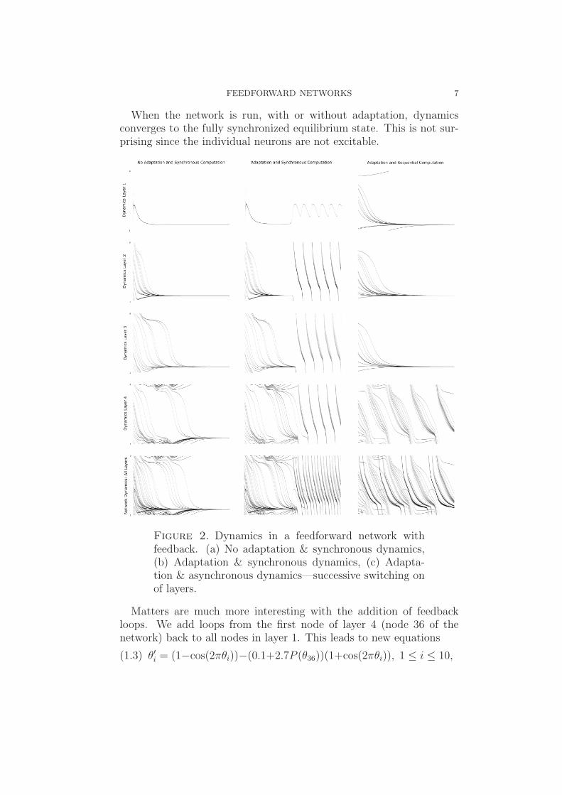
When the network is run, with or without adaptation, dynamicsconverges to the fully synchronized equilibrium state. This is not sur-prising since the individual neurons are not excitable.

Figure 2. Dynamics in a feedforward network withfeedback. (a) No adaptation & synchronous dynamics,(b) Adaptation & synchronous dynamics, (c) Adapta-tion & asynchronous dynamics—successive switching onof layers.

Matters are much more interesting with the addition of feedbackloops. We add loops from the first node of layer 4 (node 36 of thenetwork) back to all nodes in layer 1. This leads to new equations

(1.3) θ′i = (1−cos(2πθi))−(0.1+2.7P (θ36))(1+cos(2πθi)), 1 ≤ i ≤ 10,


for the nodes in layer 1 (we continue to assume the constants ηi =−0.1). The weight −2.7 is fixed in what follows and is not subject toadaptation. In Figure 2 we show numerical simulations of the dynam-ics under various assumptions but always using 4th order Runge-Kutta(Euler for the adaptation). In Figure 2(a), we show dynamics for thenetwork (with feedback) under the assumption that weights are con-stant (no adaptation). In this case, after an initial transient, there israpid convergence to a steady state solution in all layers. We show thefirst 4.07 seconds of time evolution (time step 0.002). In Figure 2(b),we show dynamics for the network with feedback and adaptation. Theresults are now quite different and all layers are approximately peri-odic. Exactly the same initialization is used as in (a) (we show the first4.07 seconds of time evolution, time step 0.002). In Figure 2(c), withthe same initialization as in (a,b), we run the dynamics asynchronouslyand with adaptation. First we switch on level 1, then add level 2, thenlevel 3 and finally, level 4. Each step was run for 2.035 seconds (timestep of 0.001). The result is surprising—when level 4 is switched onthe network shows strong periodic behaviour though this collapses atthe end of the run and converges to an equilibria state as in case (a).Finally, we ran the network sequentially with adaptation: layer 1 first,then layer 2 only, concluding with layer 4. In this case, the eventualoutcome (not shown) is the same as in Figure 2(a), though with shortertransients. In both cases (a,b), we see that the feedforward structurecan amplify transients—typically undesirable behaviour. Even if werun the network partially asynchronously, as in (c), there may still beunexpected periodic behaviour. Only in the fourth case when we runthe network sequentially, do we avoid periodic behaviour. Of course,from the point of data or image processing, there seems to be littleadvantage in running the network synchronously: all the transient dy-namics generated by each layer is fed immediately into the followinglayer.Different initializations of network and weights, as well as variation

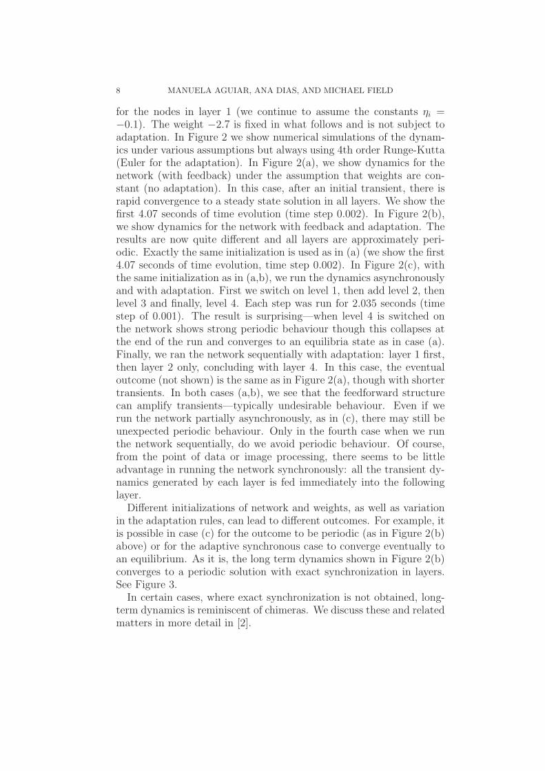
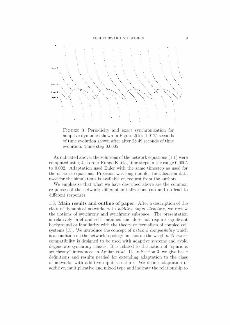
in the adaptation rules, can lead to different outcomes. For example, itis possible in case (c) for the outcome to be periodic (as in Figure 2(b)above) or for the adaptive synchronous case to converge eventually toan equilibrium. As it is, the long term dynamics shown in Figure 2(b)converges to a periodic solution with exact synchronization in layers.See Figure 3.In certain cases, where exact synchronization is not obtained, long-

term dynamics is reminiscent of chimeras. We discuss these and relatedmatters in more detail in [2].


Figure 3. Periodicity and exact synchronization foradaptive dynamics shown in Figure 2(b): 1.0175 secondsof time evolution shown after after 28.49 seconds of timeevolution. Time step 0.0005.

As indicated above, the solutions of the network equations (1.1) werecomputed using 4th order Runge-Kutta, time steps in the range 0.0005to 0.002. Adaptation used Euler with the same timestep as used forthe network equations. Precision was long double. Initialization dataused for the simulations is available on request from the authors.We emphasise that what we have described above are the common

responses of the network; different initializations can and do lead todifferent responses.

1.3. Main results and outline of paper. After a description of theclass of dynamical networks with additive input structure, we reviewthe notions of synchrony and synchrony subspace. The presentationis relatively brief and self-contained and does not require significantbackground or familiarity with the theory or formalism of coupled cellsystems [15]. We introduce the concept of network compatibility whichis a condition on the network topology but not on the weights. Networkcompatibility is designed to be used with adaptive systems and avoiddegenerate synchrony classes. It is related to the notion of “spurioussynchrony” introduced in Aguiar et al. [1]. In Section 3, we give basicdefinitions and results needed for extending adaptation to the classof networks with additive input structure. We define adaptation ofadditive, multiplicative and mixed type and indicate the relationship to


adaptation and learning rules used in neuroscience. Theorem 3.3 givesconditions for synchrony preservation; in particular that synchrony isalways preserved under multiplicative adaptation. In Section 4, wereview the definition of layered structure and feedforward networks [1]and define a feedback structure on a feedforward network—for us, thiswill almost always be a set of connections from the last layer to the firstlayer of the network. Theorem 4.15 gives a description of the possiblesynchrony for a feedforward network with feedback structure under theassumption that there are no self-loops (the network is not recurrent—an FFNN in the terminology of [1]). A consequence of this result is thatit is possible for synchrony to have a periodic structure across layerswhich cannot happen if there is no feedback [1]. Theorem 4.29 describesthe possible synchrony for a feedforward network with feedback if weallow self-loops in the first layer (an AFFNN [1]). We conclude withsome remarks on more general feedback structures with feedback fromthe last layer to intermediate layers.

2. A class of networks with additive input structure

2.1. Dynamical networks with additive input structure. Weconsider a class of dynamical networks N consisting of k interactingdynamical systems, where k ≥ 2. We label the individual dynamical

systems, or nodes, in N , by kdef= {1, . . . , k}. Thus i ∈ k will denote

the ith node of the network. We assume that the uncoupled nodeshave identical dynamics and phase space. Specifically, each node willhave phase space M (a differential manifold, possibly with boundary),and there will exist a C1 vector field f on M such that the intrinsicdynamics on node i is given by

xi = f(xi), i ∈ k.

Note our convention that the state of node i is denoted by xi. Inour examples, M will be [0, 1], R, T = R/Z, or S1 = R/2πZ (unitcircle). This gives the simplification that we can regard the dynamicsand coupling as being given by real valued functions since in these casesthe tangent bundle is trivial: TM = M × R.Associated to the network N there will be a k× k adjacency matrix

A = A(N ) = [Aij ]. Each Aij ∈ {0, 1} and the matrix A defines aunique directed graph Γ = Γ(N ) on the nodes k according to the rulethat j→i is a connection from j to i if and only if Aij = 1. If i 6= j andAij = 1, i, j are adjacent nodes. We always assume that Γ is connectedin the sense that we cannot write Γ = Γ1 ∪ Γ2 where Γ1,Γ2 are graphson complementary proper subsets of k. Define a = aA =

∑

(i,j)∈k2 Aij


and note that k − 1 ≤ a ≤ k2 (the first inequality follows since Γ isconnected). We say that N has no self-loops if Aii = 0 for all i ∈ k. IfAii = 1, then node i has a self-loop.The space M(k) of k× k real matrices may be identified with Rk2—

map [mij ] to (mij) = (m11,m12, . . . ,m1k,m21, . . . ). Using this identifi-cation, the adjacency matrix A naturally defines a subspace

W = W (A) = {w = (wij) | wij = 0 if Aij = 0}

of Rk2 . Obviously, dim(W ) = aA. We refer to W as the weight spacefor the adjacency matrix A. Note that wij may be zero if Aij = 1 butthat wij is always zero if Aij = 0.Fix a C1 coupling function φ : M2→TM satisfying φ(x,y) ∈ TyM

for all x,y ∈ M . Note that if M is a subset of Rm or Tm, we mayassume φ : M2→Rm.Under the assumption of constant weights, dynamics on N will be

defined by the system

(2.4) xi = f(xi) +k

∑

j=1

wijφ(xj,xi), i ∈ k,

where w = (wij) ∈ W—the weight space for A.

Remark 2.1. System (2.4) has an additive input structure [12, 4, 1].In particular, we can naturally add and subtract connections withoutdestroying the underlying network structure and dynamics. This iscrucial here where weights may evolve and become zero—effectivelychanging the adjacency matrix. We remark that the assumption oflinear input structure is needed for the reduction of weakly coupled non-linear oscillators to the Kuramoto phase oscillator equations [24, 20].Indeed, without that assumption, the reduced model is easily seen notto be a network of phase oscillators with diffusive coupling (see forexample [3]).

2.2. Synchrony subspaces. Let P = {Pa | a ∈ s} be a partition of k.We refer to the subsets Pa as parts of P . Let pa denote the cardinalityof Pa, a ∈ s. If s = k, we refer to P as the asynchronous partition—allparts of P are singletons—and denote the partition by A. If P is notasynchronous, then pa ≥ 1 for all a ∈ s, and s < k (so that at leastone part contains more than one element). After a relabelling of nodes,we may assume that P1 = {1, . . . , p1}, P2 = {1 + p1, . . . , p1 + p2} andso on up to Ps = {1 +

∑s−1i=1 pi, . . . , k =

∑s

i=1 pi}. We often make thisassumption in proofs.


Definition 2.2. Suppose network dynamics given by (2.4) (M , f andφ are completely general, but the weights and adjacency matrix Aare fixed). Let P = {Pa | a ∈ s} be a partition of k. For a, b ∈ sdefine the local valency function νP

a,b = νa,b : Pa→R and local in-degree

ρPa,b = ρa,b : Pa→N by

νa,b(i) =∑

j∈Pb

wij, ρa,b(i) =∑

j∈Pb

Aij, i ∈ Pa.

If s = 1 and P = {k}—the fully synchronous partition—set ν1,1 =ν : k→R, ρ1,1 = ρ : k→Z+

0 and refer to ν and ρ as the valency andin-degree.

Given the partition P , define the subspace ∆P(M) of Mk by

∆P(M) =

{

{(x1, . . . ,xk) | xi = xj if i, j ∈ Pa, some a ∈ s}, P 6= A.

Mk, if P = A.

In the coupled cell network literature [37, 16, 15], ∆P(M) is usuallycalled a polydiagonal subspace of Mk. Polydiagonal subspaces are thenatural class of subspaces to consider for the study of exact synchro-nization. Specifically, if∆P(M) is an invariant subspace for the dynam-ics of (2.4), then every solution X(t) = (x1(t), . . . ,xk(t)) of (2.4) withinitial condition in∆P(M), will consist of s groups of synchronized tra-jectories: for all a ∈ s, the trajectories xi(t), i ∈ Pa, will be identical.After relabelling of nodes (see above), we may writeX = (xp1

1 , . . . ,xpss ),

where xp ∈ ∆(Mp) is shorthand for x repeated p times.If, given w ∈ W , ∆P(M) is an invariant subspace for all choices

of f and φ in (2.4), we call P a synchrony class of N and ∆P(M) asynchrony subspace (of Mk). We emphasise that we do not vary theweights (yet).

Remark 2.3. In the coupled cell literature, it is common to regard eachpart Pa ∈ P as being associated to a colour. With this convention,nodes are synchronized if and only if they have the same colour, thatis belong to the same part. The convention in this work is that nodeslie in the same part if and only if they are synchronous ; nodes that arenot synchronous are asynchronous.

We want to give a necessary and sufficient condition for a partitionto be a synchrony class. As this will be a little different from what isgiven in [1]—we need to allow for variation in the weights—we preferto avoid the generality of the coupled cell network formalism [15], andinstead give a brief presentation that requires minimal prerequisites.


Proposition 2.4. (Notation and assumptions as above.) Given w ∈W , the partition P = {Pa}a∈s is a synchrony class of N iff each localvalency function νa,b is constant.

Proof. Sufficiency. Let ta,b denote the constant value of νa,b. Let N (P)denote the network with s nodes and dynamics given by

(2.5) ya = f(ya) +∑

b∈s

ta,bφ(yb,ya), a ∈ s,

where each node has state space M (as in (2.4)). Clearly every solutionof (2.5) determines a solution to (2.4) lying in ∆P(M) and with initialcondition (yp1

1 (0), . . . ,ypss (0)) ∈ ∆P(M). It follows by uniqueness of

solutions that every solution X(t) of (2.4) with initial condition X(0) ∈∆P(M) is of this form and so X(t) ∈ ∆P(M) for all t.Necessity. Suppose that να,β is not constant for some pair (α, β) ∈ s2.

Necessarily pα > 1. It suffices to find a specific equation of the form(2.4) for which ∆P(M) is not an invariant subspace. For this, takeM = R, f ≡ 0. Taking xa = a, a ∈ s, choose any smooth φ : R2→R

such that φ(x, y) = 1, for (x, y) near (α, β), and φ(x, y) = 0 for valuesof (x, y) near (a, b) 6= (α, β). Pick i, j ∈ Pα such that να,β(i) 6= να,β(j).Suppose xi(0) = xj(0) = α. The equations for xi,xj near t = 0 are

xi = να,β(i), xj = να,β(j).

It follows from our assumptions on φ and choice of i, j that xi(t) 6= xj(t)for t close to zero, t 6= 0. Hence P cannot be a synchrony class. �

Remark 2.5. In the coupled cell literature [16, 15], the network (2.5) isreferred to as a quotient network of (2.4). The quotient network givesdynamics on the synchrony subspace.

2.3. Network compatibility.

Definition 2.6. The partition P is network compatible if for all a, b ∈ s,either ρa,b ≡ 0 or ρa,b is non-vanishing on Pa. Let ncp(N ) denote theset of all network compatible partitions for N .

Remarks 2.7. (1) Henceforth we always assume partitions are networkcompatible. Note that the asynchronous partition A ∈ ncp(N ).(2) Our definition of network-compatible is related to, but not the sameas, the notion of spurious synchrony [1, Definition 2.9]. We emphasizethat network compatibility depends on the network topology and noton the choice of weight vector.

The asynchronous partition is the finest network compatible par-tition. The next lemma shows that there is a coarsest partition in


ncp(N ). This partition gives the maximally synchronous subspace ofMk that can be defined by a network compatible partition.

Proposition 2.8. If T is the partition associated to the polydiagonalsubspace

⋂

P∈ncp(N )

∆P(M),

then T ∈ ncp(N ).

Proof. Let T = {Ta | a ∈ s}. Then c, d ∈ Ta if and only if we can finda sequence c = c0, c1, . . . , cr = d such that for each i ∈ r, there existP ∈ ncp(N ), P ∈ P , such that ci−1, ci ∈ P . Since each partition P isnetwork compatible, it follows easily from this characterisation of theparts of T , that T is network compatible. �

Remark 2.9. In more abstract terms, Proposition 2.8 follows from theexistence of a complete lattice structure on ncp(N ). See Stewart [36]for the lattice structure on synchrony classes in coupled cell systemsand Davey and Priestley [10] for background on lattices. In terms ofthe lattice structure on ncp(N ), T is the top (maximal) element and Ais the bottom (minimal) element. In our context, it straightforward todefine the join operation in terms of operations on partitions (what isused in the proof of Proposition 2.8 to obtain the top element) and wedo not have to be concerned about the definition of the meet operationwhich does not generally correspond to the intersection operation onpartitions.

For w ∈ W , define

sync(N ,w) = {P ∈ ncp(N ) | P is a synchrony class}.

Note that A ∈ sync(N ,w) and that sync(N ,w) will generally be aproper subset of ncp(N ).

Lemma 2.10. Given w ∈ W ,

V (w) = {u ∈ W | sync(N ,u) ⊇ sync(N ,w)},

is a vector subspace of W .

Proof. Obvious. �

Remark 2.11. If u ∈ V (w), then we may have sync(N ,u) ) sync(N ,w).For example, if u = 0. On the other hand, sync(N ,u) = sync(N ,w)for u in an open dense subset of V (w).


Suppose P = {Pa}a∈s ∈ ncp(N ). For a, b ∈ s, let W (a, b) denote the(∑

i∈a,j∈b Aij)-dimensional subspace of W corresponding to all possible

weights wa,b = (wij), with i ∈ Pa, j ∈ Pb. If w ∈ W , let wa,b ∈ W (a, b)denote the projection of w in W (a, b). For t ∈ R, define

W (a, b)(t) = {wa,b ∈ W (a, b) | νa,b(i) =∑

j∈Pb

wij = t, all i ∈ Pa}.

Lemma 2.12. Let P = {Pa}a∈s ∈ ncp(N ). For all a, b ∈ s, t ∈ R,W (a, b)(t) 6= ∅.

Proof. The network compatibility condition on P implies that if thelocal in-degree ρa,b 6≡ 0, then for all t ∈ R, i ∈ Pa,

∑

j∈Pbwij = t has

solutions. �

Definition 2.13. Let P = {Pa}a∈s ∈ sync(N ,w). The local valenciesνa,b are non-degenerate if νa,b is non-vanishing whenever ρa,b is notidentically zero.

Theorem 2.14. Let ε > 0 and w ∈ W be a weight vector for N .

(1) If P = {Pa}a∈s ∈ sync(N ,w), P 6= A, then we can chooseweight vectors w′,w′′ such that(a) ‖w − w′‖ < ε, the local valencies νa,b for w′ are non-

degenerate, and P ∈ sync(N ,w′).(b) All weights w′′

ij, with Aij = 1, are strictly positive and P ∈sync(N ,w′′).

(2) We may choose weight vectors w′, w′′ such that(a) sync(N ,w′) = sync(N ,w), ‖w−w′‖ < ε, and local valen-

cies for w′ are non-degenerate.(b) sync(N ,w′′) = sync(N ,w), and w′′ is strictly positive

(w′′ij > 0, if Aij = 1).

Remark 2.15. Theorem 2.14 shows that for network compatible par-titions P , we can always perturb the weights so that P is a non-spurious synchrony class—the local valencies are non-degenerate [1].Note that if the weight vector is strictly positive, as in (1,2)(b), thenthe non-identically zero local valencies are strictly positive and so non-degenerate.

Proof of Theorem 2.14 (1) Both statements follow easily fromLemma 2.12. We indicate the proof of (1b). For each a, b ∈ s, i ∈ a,j ∈ b, define

w′′ij =

{

0 if ρa,b ≡ 01

ρa,b(i)otherwise.


For this choice of w′′, the non-identically zero local valencies νPa,b are

all constant, equal to 1.(2) Since not being a specific synchrony class is an open property onthe set of weights, we may choose an open neighbourhood U of w suchthat for all u ∈ U , sync(N ,u) ⊆ sync(N ,w) (see Lemma 2.10 andnote that if u ∈ V (w) ∩ U , then sync(N ,u) = sync(N ,w)).Let T ∈ ncp(N ) be the partition given by Proposition 2.8. Apply-

ing the argument of the proof of (1b) with P = T , choose a strictlypositive weight vector w⋆ such that the local valencies νT

a,b are all non-degenerate. Since every P ∈ ncp(N ) is a refinement of T , the localvalencies νP

a,b for w⋆ are non-degenerate for all P ∈ sync(N ,w). Con-

sider the weight vector w⋆λ = w⋆ + λw, λ ∈ R. By Lemma 2.10,

sync(N ,w⋆λ) ⊇ sync(N ,w), for all λ ∈ R. For sufficiently large λ,

sync(N ,w⋆λ) = sync(N ,w) (since λ−1w⋆ + w ∈ U). Consequently,

sync(N ,w⋆λ) = sync(N ,w), λ 6= 0. Hence we can choose λ0 ∈ R so

that sync(N ,w⋆λ0) = sync(N ,w), local valencies are non-degenerate

and w⋆λ0

is strictly positive. Take w′′ = w⋆λ0

to complete the proof of(2b). For (2a), choose µ0 ∈ [0, ε/‖w⋆‖) so that w′ = w + µ0w

⋆ ∈ Uand local valencies are non-degenerate. �

Example 2.16. If N is a network with an all-to-all coupling adjacencymatrix (no self-loops), then all partitions are network compatible. Hereit is easy to see that if all weights are equal, then all partitions aresynchrony classes.

Remark 2.17. For network compatible partitions, we allow zero localvalency when the local in-degree is non-zero. It follows from Theo-rem 2.14(2) that network compatibility allows us to choose a synchronypreserving perturbation of the weight vectors making all local valenciesnon-degenerate.

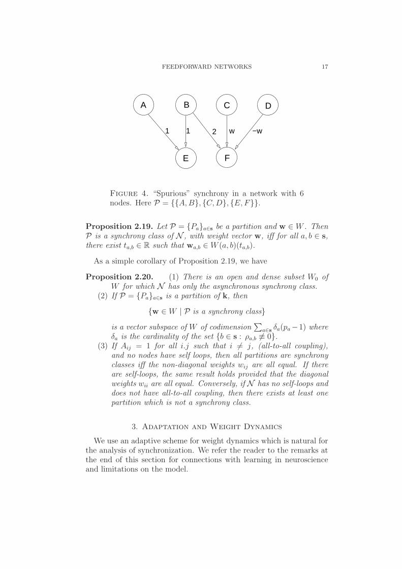
Examples 2.18. (1) The partition P = {{A,B}, {C,D}, {E,F}},and assigned weight vectors, shown in Figure 4, define an invariantsubspace ∆P(M). However, there are no connections from nodes C,Dto E and so the partition is not network compatible and does not give asynchrony class according to our definition. Note that it is not possibleto choose weights wFC , wFD which do not sum to zero and preserve thesynchrony class.(2) Suppose that row i of the adjacency matrix ofN is zero and that rowj is non-zero. Then the nodes i and j are asynchronous. In particular,it is not possible for all the nodes in N to be synchronous ({k} is nota synchrony class).

We have the following restatement of Proposition 2.4


1 1 2 w −w

A B C D

E F

Figure 4. “Spurious” synchrony in a network with 6nodes. Here P = {{A,B}, {C,D}, {E,F}}.

Proposition 2.19. Let P = {Pa}a∈s be a partition and w ∈ W . ThenP is a synchrony class of N , with weight vector w, iff for all a, b ∈ s,there exist ta,b ∈ R such that wa,b ∈ W (a, b)(ta,b).

As a simple corollary of Proposition 2.19, we have

Proposition 2.20. (1) There is an open and dense subset W0 ofW for which N has only the asynchronous synchrony class.

(2) If P = {Pa}a∈s is a partition of k, then

{w ∈ W | P is a synchrony class}

is a vector subspace of W of codimension∑

a∈s δa(pa−1) whereδa is the cardinality of the set {b ∈ s : ρa,b 6≡ 0}.

(3) If Aij = 1 for all i.j such that i 6= j, (all-to-all coupling),and no nodes have self loops, then all partitions are synchronyclasses iff the non-diagonal weights wij are all equal. If thereare self-loops, the same result holds provided that the diagonalweights wii are all equal. Conversely, if N has no self-loops anddoes not have all-to-all coupling, then there exists at least onepartition which is not a synchrony class.

3. Adaptation and Weight Dynamics

We use an adaptive scheme for weight dynamics which is natural forthe analysis of synchronization. We refer the reader to the remarks atthe end of this section for connections with learning in neuroscienceand limitations on the model.


First, assume weights and dynamics evolve according to

xi = f(xi) +k

∑

j=1

wijφ(xj,xi), i ∈ k,(3.6)

wij = ϕ(wij,xi,xj), (i, j) ∈ N,(3.7)

where N = {(i, j) ∈ k2 | Aij = 1}, (3.6) satisfies the conditions for(2.4), and ϕ : R×M2→R is C1. This model for dynamics and adapta-tion assumes that the evolution of the weight wij depends only on wij

and the states of the nodes i and j.In what follows, we assume for simplicity that solutions of (3.6,3.7)

are defined for all t ≥ 0.

Definition 3.1. The system (3.6,3.7) preserves synchrony if given apartition P and weight initialization w0 ∈ W such that P is a syn-chrony class of (3.6) with w = w0, then for every solution (x(t),w(t))of (3.6,3.7) with initialization x(0) ∈ ∆P(M), w(0) = w0, we havex(t) ∈ ∆P(M), all t ≥ 0.

Of course, without further conditions, (3.6,3.7) will not preserve syn-chrony.

Definition 3.2. (1) Adaptation is multiplicative if there is a C1

map Φ : M2→R such that

ϕ(w,x,y) = wΦ(x, y), (w, (x,y)) ∈ R×M2.

(2) Adaptation is additive if there is a C1 map Φ : M2→R suchthat

ϕ(w,x,y) = Φ(x, y), (w, (x,y)) ∈ R×M2.

(3) Adaptation is of mixed type if there are distinct C1 maps Φ,Ψ :M2→R and C 6= 0 such that

ϕ(w,x,y) = wΦ(x,y) + (C − w)Ψ(x,y), (w, (x,y)) ∈ R×M2.

Theorem 3.3. (Notation and assumptions as above.)

(1) If adaptation is multiplicative, then (3.6,3.7) preserves syn-chrony.

(2) If adaptation is additive or of mixed type, then (3.6,3.7) pre-serves a synchrony class {Pa}a∈s provided that the local in-degree functions ρa,b are constant for all a, b ∈ s.

Proof. The proof is similar to that of Proposition 2.4. We give detailsfor (1). Suppose that for the weight vector w0, P is a synchrony classfor (3.6). Necessarily νa,b will be constant functions for all a, b ∈ s for(3.6) (no adaptation). Fix x0 ∈ ∆P(M).


Initialize (3.6,3.7) at w0 and x0 ∈ ∆P(M).Consider the ‘quotient’ system

ya = f(ya) +∑

b∈sVa,bφ(yb,ya), a ∈ s,(3.8)

Va,b = Va,bΦ(yb,ya), a, b ∈ s,(3.9)

wij = wijΦ(yb,ya), a, b ∈ s, i ∈ Pa, j ∈ Pb,(3.10)

where ya ∈ M , a ∈ s, and Va,b : R→R, a, b ∈ s. Observe that if weinitialize weights with w0, and set Va,b(0) = νa,b =

∑

j∈Pbw0

ij, where i ∈Pa, a, b ∈ s, then the solution to (3.9) is given by Va,b(t) =

∑

j∈Pbwij(t),

a, b ∈ s, any i ∈ Pa.Suppose x0 = (xp1

1 , . . . , xpss ) ∈ ∆P(M). Initialize (3.8,3.9,3.10) at

y0 = (x1, . . . , xs) ∈ M s, w0, and Va,b(0) = νa,b, a, b ∈ s. Then x(t) =(yp1

1 (t), . . . ,ypss (t)), (wij(t)) will solve

xi = f(xi) +∑

b∈s

(∑

j∈b

wijφ(xj,xi)), i ∈ k,(3.11)

wij = wijΦ(xi,xj), (i, j) ∈ N.(3.12)

We showed above that the solution to (3.9) is given by Va,b(t) =∑

j∈Pbwij(t), a, b ∈ s, for any i ∈ Pa and so, by Proposition 2.4,

∑

j∈b wij = Va,b is independent of i ∈ Pa for all a, b ∈ s. Hence syn-chrony is preserved. �

Remarks 3.4. (1) The models we have used for weight dynamics arepartly motivated by models for (unsupervised) learning in neuroscience—most notably Hebbian learning rules [8, 7]: “neurons that fire to-gether wire together”—and related models for synaptic plasticity suchas Spike-Timing Dependent Plasticity [13, 8, 31]. These models arelocal in the sense that the dynamics of a weight depends only on theweight and the nodes at the end of the associated connection and donot optimise or constrain a ‘global’ quantity such as

∑

ij wij (as is done,

for example, in the work of Ito & Kaneko [23, 21, 22]).(2) In practice, it is customary to assume weights are positive and soweight dynamics will be constrained to the positive orthant Ra

+. Thisis no problem for adaptation which is multiplicative or of mixed type(with appropriate conditions). However, for additive adaptation, hardlower and upper bounds are typically required. If weights saturate,synchrony is usually lost. If we restrict to positive weights, then thereare no issues with spurious synchrony (see [1] and note also Theo-rem 2.14(2b)). If the local in-degrees are all constant with the samevalue, we can make all weights strictly positive and preserve synchronyby a weight translation wij→wij + C, C independent of i, j. If we


allow negative weights then a local valency νa,b which is zero will bepreserved under adaptation of multiplicative type and so, following [1],spurious synchrony is conserved. This is not generally so for adaptationof mixed type and almost never true for adaptation of additive type.Since weight dynamics, with multiplicative or additive adaptation, of-ten leads, in the limit, to zero weights, and hence zero local valencies,we prefer not to impose restrictions on spurious synchrony other thanto require partitions are network compatible; rather, we identify whensynchrony results because of a zero local valency.

4. Layered structure and feed forward networks

We continue to follow the notational conventions and terminologydeveloped in section 2. Thus N will be a connected network consistingof k nodes, an adjacency matrix A, an associated connected networkgraph Γ and weight vector w ∈ W . Dynamics will be given accordingto (2.4).

Definition 4.1 ([1, Definition 3.1]). The network N has a layeredstructure L = {Lt}t∈ℓ if we can partition k as k = ∪ℓ

t=1Lt, where

(a) ℓ > 1.(b) The only connections to nodes in L1 are self-loops.(c) If i ∈ Lt, t > 1, then Aiu = 1 only if u ∈ Lt−1. In particular,

no node receives a connection from a node in Lℓ.(d) Every node in ∪ℓ

t=2Lt receives at least one input.(e) Every node in ∪ℓ−1

t=1Lt has at least one output.

We refer to Lt as the tth layer of N .

Suppose that the network N has a layered structure with layersL1, . . . ,Lℓ. Following [1], N is a Feed-Forward Neural Network—FFNNfor short—if nodes in L1 have no self-loops, andN is an Auto-regulationFeed-Forward Neural Network—AFFNN for short—if at least one nodein L1 has a self-loop. A description of synchrony classes for (A)FFNNs,with examples, is given in [1, §§3,4].If N is an (A)FFNN and the partition P is a synchrony class, we

have induced partitions Pt = P ∩ Lt, t ∈ ℓ. It follows from [1] that ifN is an FFNN, there is no pair of induced partitions with synchronousnodes. That is, for an FFNN synchronization occurs within but notbetween layers.

Proposition 4.2. (Notation and assumptions as above.) Suppose thatN is an adaptive (A)FFNN with layers L1, . . . ,Lℓ and that the partitionP is a synchrony class for the initial weight vector w0. Set Pt = Lt∩P,t ∈ ℓ.


(1) If adaptation is multiplicative, then the synchrony will be pre-served within layers. That is, the induced partitions Pt are pre-served for all t ∈ ℓ.

(2) If adaptation is of mixed or additive type and the local in-degreesρa,b are constant on layers, then synchrony will be preservedwithin layers.

Proof. (1) follows from Theorem 3.3. (2) uses Theorem 3.3 and an easyinduction on layers. �

Remarks 4.3. (1) We consider dynamics on adaptive (A)FFNNs in part2 [2]. As part of this we will consider both synchronous dynamics—dynamical evolution of the network in the standard way—and asyn-chronous evolution. For this we successively switch on layers whenthreshold conditions are met on previous layers. This is both similarto the way a discrete artificial neural net works and analogous to theway production and inventory control networks are operated (we referto [4, 5] for details on asynchronous and functional networks).(2) From an evolutionary point of view, a feedforward network can beconsidered as a relatively primitive object. Under evolutionary pres-sure, the network will optimise a function. This may entail the appear-ance of feedback loops in the network. The bifurcations resulting fromthe addition of feedback loop(s) to a feedforward network are subtleand related to phenomena such as the bull-whip effect in productionand inventory control [25]. For the remainder of this work, we considerhow feedback loops affect synchrony in feedforward networks. In part2 [2], we investigate bifurcation and dynamics for both non-adaptiveand adaptive networks of feedforward type.

4.1. Notation and assumptions. Throughout this section, N willdenote a network with layered structure L = {Lt}t∈ℓ.

Definition 4.4. A transversal (for N ) is a path n1→n2→ . . .→nℓ inthe network graph Γ such that nt ∈ Lt, t ∈ ℓ. The network N isfeedforward connected if there is a transversal joining any node in L1

to any node in Lℓ.

Remark 4.5. Since every node in N r L1 has at least one input (Defi-nition 4.1(d)), it follows (Definition 4.1(c,e)) that if j ∈ N , then j lieson at least one transversal through N .

4.2. Feedback structures on an (A)FFNN. Henceforth assumethat N is a feedforward connected (A)FFNN.

Definition 4.6. Let N have layers {Lt}t∈ℓ and J be a non-emptysubset of {1, . . . , ℓ − 1}. A J-feedback structure F on N consists of


a non-empty set of connections from nodes in Lℓ to nodes in ∪t∈JLt,together with a corresponding weight vector u lying in the associatedweight space U for the feedback loops.

Remark 4.7. Here we focus almost exclusively on {1}-feedback struc-tures and henceforth refer to a {1}-feedback structure as a feedbackstructure. At the end of the section there are some comments on{2, . . . , ℓ− 1}-feedback structures.

Definition 4.8. Let F be a feedback structure on N .

(1) F is of type A if every node in L1 receives at least one connectionfrom a node in Lℓ.

(2) F is of type B if every node in Lℓ is connected to at least onenode in L1.

(3) F is of type C if it is of type A and B.

If F is a feedback structure on N , let N ⋆ denote the associatednetwork. Note that N and N ⋆ have the same node set. If F is of typeA, we say N ⋆ is of type A. Similarly for types B and C.

Lemma 4.9. Let F be a feedback structure on N . There exists amaximal feedforward connected subnetwork Nc of N such that

(1) F is a feedback structure of type B on Nc.(2) i ∈ k is a node of Nc iff there is a transversal (in N ) containing

i and ending at a node in Lℓ connected to a node in L1.(3) i→j is a connection for Nc iff i→j is a segment of a transversal

(in N ) containing i, j and ending at a node in Lℓ connected toa node in L1.

(4) If N ⋆ is of type A, then N ⋆c will be of type C and the node set

of Nc contains all nodes in L1.

Proof. Define the network graph of Nc ⊂ N to be the union of alltransversals joining nodes in L1 to nodes in Lℓ which connect to nodesin L1. Obviously, Nc is feedforward connected, satisfies (2,3), and Fdefines a feedback structure of type B on Nc. �

Remark 4.10. For FFNNs (as opposed to AFFNNs), we usually assumefeedback structures are of type A. It follows from Lemma 4.9, that forthe study of feedback induced synchrony on networks N ⋆ of type A, itis no loss of generality to assume N ⋆ of type C. Indeed, once we havesynchrony for N ⋆

c , it is easy to extend to N ⋆ as the extension will notbe constrained by the feedback structure.

Lemma 4.11. (Notation and assumptions as above.) Suppose F is afeedback structure of type C on N . Given i ∈ Lt, j ∈ Lu, there exists


a path γ : i = i0→i1→ . . .→ip = j in the network graph of N ⋆. Theminimal length p of γ is dℓ + u − t, where d ∈ {0, 1, 2}, if u ≥ t, andd ∈ {1, 2} otherwise.

Proof. A straightforward computation using feedforward connectednessand Remark 4.5. �

4.3. Synchrony for FFNNs with feedback structure. We con-tinue with the assumptions and notation of the previous section andemphasize that N is always assumed feedforward connected.

Definition 4.12. Let P = {Pa}a∈s be a synchrony class for N ⋆ andsuppose d ∈ [1, ℓ−1] is a factor of ℓ and P 6= {k}—the fully synchronouspartition.

(1) P is layer d-periodic (or layer periodic, period d) if, for all a ∈ s,and t, u ∈ ℓ.

Pa ∩ Lt 6= ∅ =⇒ Pa ∩ Lu 6= ∅, t ≡ u, mod d.

(d is assumed minimal for this property.)(2) If P is layer 1-periodic, P is layer complete.

Remark 4.13. If P is layer periodic, then each node in Lt will be syn-chronized with nodes in other layers. If P is layer complete, then eachnode in Lt will be synchronized with nodes in every other layer. Inparticular, since a layer complete partition is not the fully synchronouspartition, each layer of N contains at least two nodes.

Examples 4.14. (1) In Figure 5 we show two examples of layer peri-odic synchrony classes for feedforward connected FFNNs with feedbackstructure. Connections are labelled with weights and weights are arbi-trary real numbers with the proviso that weights with the same symbolmust have the same value.In Figure 5(b), if we move the outputs from the top node in L4

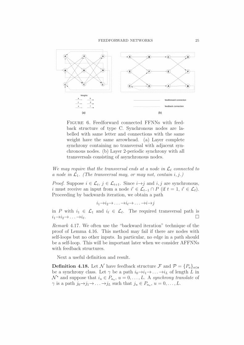
labelled A to the other node labelled A in L4, P is still layer com-plete. However, the feedback structure is no longer of type B. As inLemma 4.9, we can remove the node without outputs and the two nodeslabelled B in the first row, together with associated 6 connections, toarrive at a 9-node network. The resulting feedback structure is of typeC and the network is layer complete.(2) Figure 6(a) gives an example of layer complete synchrony P suchthat there are no adjacent synchronous nodes: if the weight sums a+e,b + d and c + f are distinct, then nodes labelled A,B,C are pairwiseasynchronous and so there are no edges between synchronous nodes.Figure 6(b) gives an example of layer 2-periodic synchrony such thatno transversal consists of synchronous nodes.


α2

α1

α1 α2+

µ

ρ

ρ

γ

γ

δ δ

ρ

µ

β

µ

β

A AB

B

B

C CD D

feedback connection

feedforward connection

A A

A

A

A

A

A

B

B

B

B

B

B

α

α

γ

γ

γ

αγ β δ

δ

δβ

β

β

δ

β

αγ

γ

δ

α

β

γβδαδ

β

α

α

δ

γ

B

B

A

(a) (b)

Figure 5. Both networks shown are feedforward con-nected FFNNs with feedback structure of type C.Weights are denoted α, β, . . . ∈ R and nodes with sameletter are synchronized. (a) Layer 2-periodic networksynchrony class. (b) Layer complete network synchronyclass.

Theorem 4.15. (Notation and assumptions as above.) Suppose Nhas feedback structure F of type B. If P is a synchrony class for N ⋆

such that there exists P ∈ P containing nodes from different layers,then

(1) If P contains nodes i, j from adjacent layers, P is layer completeor the fully synchronous partition. If, in addition, P containsan edge i→j, then P contains a transversal.

(2) If P only contains nodes from non-adjacent layers, then P islayer d-periodic, d > 1.

(3) F is of type A.

Conversely, if P is a synchrony class then either (a) P is layer periodic,or (b) only nodes in the same layer can synchronize, or (c) all nodesare synchronous, or (d) all nodes are asynchronous. In cases (a,c), Fmust be of type A; in cases (b,d) F may or may not be of type A.

The proof of Theorem 4.15 depends on a number of subsidiary resultsof interest in their own right.

Lemma 4.16. Let N have feedback structure F and P be a synchronyclass for N ⋆. If there exists P ∈ P which contains nodes i, j, withi→j, then there exists a transversal consisting entirely of nodes in P .


A B

B

C

C

D

AD

E F E F

A

B

C

A A

C C

B B

a

c

e

b

d

f

Weights

feedforward connection

feedback connection

(a) (b)

Figure 6. Feedforward connected FFNNs with feed-back structure of type C. Synchronous nodes are la-belled with same letter and connections with the sameweight have the same arrowhead. (a) Layer completesynchrony containing no transversal with adjacent syn-chronous nodes. (b) Layer 2-periodic synchrony with alltransversals consisting of asynchronous nodes.

We may require that the transversal ends at a node in Lℓ connected toa node in L1. (The transversal may, or may not, contain i, j.)

Proof. Suppose i ∈ Lt, j ∈ Lt+1. Since i→j and i, j are synchronous,i must receive an input from a node i′ ∈ Lt−1 ∩ P (if t = 1, i′ ∈ Lℓ).Proceeding by backwards iteration, we obtain a path

i1→i2→ . . .→iℓ→ . . .→i→j

in P with i1 ∈ L1 and iℓ ∈ Lℓ. The required transversal path isi1→i2→ . . .→iℓ. �

Remark 4.17. We often use the “backward iteration” technique of theproof of Lemma 4.16. This method may fail if there are nodes withself-loops but no other inputs. In particular, no edge in a path shouldbe a self-loop. This will be important later when we consider AFFNNswith feedback structures.

Next a useful definition and result.

Definition 4.18. Let N have feedback structure F and P = {Pa}a∈sbe a synchrony class. Let γ be a path i0→i1→ . . .→iL of length L inN ⋆ and suppose that iu ∈ Pau , u = 0, . . . , L. A synchrony translate ofγ is a path j0→j1→ . . .→jL such that ju ∈ Pau , u = 0, . . . , L.


Lemma 4.19. Let N have feedback structure F and P = {Pa}a∈s be asynchrony class. Let γ be a path i0→i1→ . . .→iL in N ⋆ with ip ∈ Pap,0 ≤ p ≤ L.

(1) If jL ∈ PaL, there is a synchrony translate j0→j1→ . . .→jL withjp ∈ Pap, 0 ≤ p ≤ L.

(2) If a0 = aL, there is a synchrony translate j0→j1→ . . .→jL of γwith jL = i0. Necessarily, j0 ∈ Pa0.

Proof. (1) follows using the standard synchrony based backward itera-tion argument. Statement (2) is a special case of (1). �

Proposition 4.20. Let N have feedback structure F of type B andP = {Pa}a∈s be a synchrony class for N ⋆ with s > 1. Suppose thereexist a ∈ s and nodes i, j ∈ Pa lying in adjacent layers. Then:

(1) If i→j then Pa contains a transversal.(2) F is of type A.(3) P is layer complete or the fully synchronous partition.

Proof. (1) By Lemma 4.16, Pa contains a transversal γ.(2) F is of type B and feedforward connected. Suppose that i ∈ Lp,j ∈ Lp+1, where i, j ∈ Pa. Take a transversal containing i and leti′ ∈ Ll ∩ Pb denote the end node of the transversal. Take a synchronytranslate of this transversal through node j and note that there is anode in j′ ∈ Pb ∩ L1 belonging to this translate. Suppose there isone node k ∈ L1 not receiving at least one connection from a nodeof Ll. Take a transversal from k to i′. The synchrony class of nodek should be different from any synchrony class of the other nodes inthat transversal. Indeed, since k has no inputs, the synchrony classof k can only occur in the first layer. Take a synchrony translate ofthis transversal leading to j′. Then there is a node in L2 in the samesynchrony class as k, a contradiction. Thus F is of type A.(3) Since F is of type C, it follows from Lemma 4.11 that there is apath from i to j. A synchrony translate of this path, starting at nodej, ends at a node in Pa ∩ Lp+2. Iterating this argument, we concludethat there is at least one node from each layer in Pa. If we take anynode q ∈ Pd, with d 6= a, then we have paths from q to any of the nodesin Pa in each of the layers. Taking synchrony translates of these paths,we conclude that Pd contains nodes from every layer and so P is layercomplete or the fully synchronous partition. �

Lemma 4.21. Let N have feedback structure F which is not of typeA. If P = {Pa}a∈s is a synchrony class, then each Pa ∈ P is containedin a unique layer Li(a) of L.


Proof. Suppose the contrary. Then, for some a ∈ s, there exist i0, j0 ∈Pa with i0 ∈ Lt, j0 ∈ Lu, where t < u. Note that if t = 1 there is aconnection from Lℓ to i0—since i0, j0 are synchronous and u > 1. SinceN is feedforward connected, there is a path τ : ip→it−1→ . . .→i0, oflength either t−1 or ℓ+t−1, where ip ∈ L1 has no connections from Lℓ.By Lemma 4.19(1), there is a synchrony translate jp→jp−1→ . . .→j0of τ . But jp /∈ L1 and so has inputs. Contradiction since ip receives noinputs and so cannot be synchronous with jp. �

Before proving the final result needed for the proof of Theorem 4.15,we need a definition.

Definition 4.22. Let P = {Pa}a∈s be a synchrony class for N ⋆ anda ∈ s. If Pa only contains nodes in one layer, set δ(a) = 0, else define

δ(a) = min{|i− j| | i, j ∈ Pa, where i, j lie in different layers}.

We refer to δ(a) as the synchronization distance for Pa.

Proposition 4.23. Let N have feedback structure F of type B. If P ={Pa}a∈s is a synchrony class for N ⋆ and for some a ∈ s, δ(a) = d > 0,then

(1) F is of type A.(2) d|ℓ.(3) P is layer d-periodic and δ : s→N is constant, equal to d.

In particular, if d = 1, P is either layer complete or the fully synchro-nous partition.

Proof. Property (1) holds by Lemma 4.21. Hence, by Lemma 4.11,given any two nodes in N ⋆ there is a path connecting them. Supposem1, n1 ∈ Pa, where m1 ∈ Lu, n1 ∈ Lu+d, and u ≥ 1 is minimal forthis property. By Lemma 4.11, we may choose a path γ1 of shortestlength joining m1 to n1. If the length of γ1 is L, then L = pℓ + d,where 0 ≤ p ≤ 2. By Lemma 4.19(2), we may choose a sequence γj ofsynchrony translates of γ1 such that γj will connect mj to nj, wherenj = mj−1, j > 1. If d 6 | ℓ, then for some j > 1 either mj ∈ Lv, forv < u, or u < v < u+d. In the first case, we contradict the minimalityof u; in the second case we contradict the definition of synchronizationdistance. Hence d|ℓ, proving (2).For (3), suppose that a ∈ s is chosen so that δ(a) is minimal. Suppose

b ∈ s, b 6= a, and choose the minimal v ≥ 1 such that Lv∩Pb 6= ∅. Pickx ∈ Lv ∩ Pb and path from x to m1 ∈ Lu. Then choose a synchronytranslate of the path to connect some y ∈ Lv+d∩Pb to n1 ∈ Pa. Just asabove, we show that Lv+jd ∩ Pb 6= ∅ for all j ≥ 0. If there were nodesin other layers, this would contradict the minimality of δ(a). �


Remark 4.24. Let N ⋆ be of type B. If there is a synchrony class Pfor which there exists Pa ∈ P with δ(a) ≥ 2, then it follows fromProposition 4.23 that ℓ ≥ 4 and is not prime.

Proof of Theorem 4.15. (1) follows from Propositions 4.23(3),Proposition 4.20, and Lemma 4.16. (2) follows from Proposition 4.23(3),(3) follows from Proposition 4.23(1). The converse statements followfrom Lemma 4.21, Proposition 4.23 and Examples 4.14. �

4.4. Synchrony for AFFNNs with feedback structure. Through-out this section N will be an AFFNN with layer structure L = {Li}i∈sand F will be a feedback structure on N . Let N ⋆ denote the associatednetwork. We always assume

(1) N is feedforward connected.(2) N ⋆ is of type B.

Regarding (2), note that by Lemma 4.9 there is a maximal feedfor-ward connected subnetwork Nc of N on which F defines a connectionstructure of type B. Noting Remark 4.10, it is no loss of generality toassume N ⋆ is of type B.Type A has the meaning previously given—every node in layer 1

receives a feedback loop.We define F (or N ⋆) to be of type D if (a) there is a node in layer

1 which does not receive a feedback loop, and (b) every node in layer1 which does not receive a feedback loop has a self-loop. If (a) is truebut (b) fails, F is of type D⋆. With these conventions, an AFFNNwith feedback structure will be precisely one of types A, D or D⋆. Weemphasize that there will always be at least one feedback loop and oneself loop but that for type D⋆ networks there may be nodes with neithera feedback loop nor a self-loop.Let F be a feedback structure of type D or D⋆. For t ∈ ℓ, define

subsets Dt of Lt recursively by:

(1) D1 is the subset of L1 consisting of nodes which receive nofeedback loop.

(2) Dt is the subset of Lt consisting of nodes which only receiveconnections from nodes in Dt−1, t ≥ 2.

Let ND be the subnetwork of N with node set ND = ∪t≥1Dt and allconnections i→j ∈ N , where i, j ∈ ND.

Lemma 4.25. (Notation and assumptions as above.)

(1) There exists p < ℓ such that Dj = ∅, j > p.


(2) For t > 1, every node in Dt receives a connection from a nodein Dt−1. Moreover, no node in ND receives a connection froma node not in ND.

(3) Feedforward connected components of ND are either of type D ortype D⋆. If ND is of type D, then all the feedforward componentswill be of type D.

Proof. Immediate by feedforward connectedness and the definition ofND. �

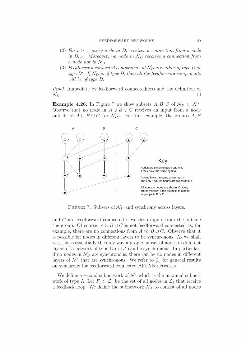
Example 4.26. In Figure 7 we show subsets A,B,C of ND ⊂ N ⋆.Observe that no node in A ∪ B ∪ C receives an input from a nodeoutside of A ∪ B ∪ C (or ND). For this example, the groups A,B

+

+ +

+

++ +

Nodes are synchronous if and onlyif they have the same symbol.

Arrows have the same arrowhead ifand only if source nodes are synchronous.

All inputs to nodes are shown. Outputsare only shown if the output is to a nodein groups A, B or C.

Key

A B C

Figure 7. Subsets of ND and synchrony across layers.

and C are feedforward connected if we drop inputs from the outsidethe group. Of course, A ∪ B ∪ C is not feedforward connected as, forexample, there are no connections from A to B ∪ C. Observe that itis possible for nodes in different layers to be synchronous. As we shallsee, this is essentially the only way a proper subset of nodes in differentlayers of a network of type D or D⋆ can be synchronous. In particular,if no nodes in ND are synchronous, there can be no nodes in differentlayers of N ⋆ that are synchronous. We refer to [1] for general resultson synchrony for feedforward connected AFFNN networks.

We define a second subnetwork of N ⋆ which is the maximal subnet-work of type A. Let F1 ⊂ L1 be the set of all nodes in L1 that receivea feedback loop. We define the subnetwork NA to consist of all nodes


and edges that belong to transversals from nodes in F1. The feed-back structure F induces a feedback structure on NA with associatednetwork N ⋆

A. Denote the node set of N ⋆A by NA.

Lemma 4.27. (Notation and assumptions as above.)

(1) NA contains all the nodes in Lℓ.(2) N ⋆

A is of type A.(3) The node sets of ND and N ⋆

A (or NA) are disjoint and compli-mentary.

(4) If P is a synchrony class for N ⋆, then PD = P ∩ND will be asynchrony class for ND. Conversely, every synchrony class ofND extends to a synchrony class of N ⋆.

Proof. For (3), observe that ND receives no inputs from N ⋆A. All the

remaining statements are routine and we omit proofs. �

Remark 4.28. If N is not of type A, then it is possible that no node inlayer 1 of NA has a self-loop. In this case, possible synchrony for NA

is constrained by Theorem 4.15. Moreover, for this case, we shall showthat nodes in N , which lie in NA, can only be synchronous if they liein the same layer. In particular, N cannot be layer periodic or fullysynchronous.

Theorem 4.29. (Assumptions and notation as above.) Let F be afeedback structure on the AFFNN N . If P = {Pa}a∈s is a synchronyclass for N ⋆ then one (at least) of the following possibilities hold.

(1) P is layer complete and F is of type A.(2) All nodes are synchronous and F is not of type D⋆.(3) All nodes are asynchronous and F is of type A, D or D⋆.(4) There exists P ∈ P such that P is contained in a layer and is

not a singleton. F can be of type A, D or D⋆.(5) If P 6= {k}, F is of type D or D⋆, and there exist synchronous

nodes i, j in different layers,(a) i, j ∈ ND and are synchronous in PD = P ∩ND.(b) If F is not of type D⋆, the partition PD may be the fully

synchronous partition of ND.(c) No node in ND can be synchronous with a node in N ⋆

A andthere are no synchronous nodes in different layers of N ⋆

A.

Remarks 4.30. (1) One only of (1–3) of Theorem 4.29 can occur andthen (4,5) do not occur. On the other hand, (4) and (5) may bothoccur multiple times for the same synchrony class. Note that if N ⋆ isof type A, then ND = ∅.(2) If no node in layer 1 of NA has a self loop, it is easy to find examples


where every layer of N ⋆ contains at least two synchronous nodes.(3) Synchrony for feedforward connected AFFNNs is classified in [1,§4] and these results can be used to enumerate synchrony classes for aspecific network ND.

The following results are corollaries of Theorem 4.29.

Corollary 4.31. Let F be a feedback structure on the AFFNN N suchthat at least one node in the first layer does not receive a feedback loop.Given a synchrony class for N ⋆, we have precisely one of the followingpossibilities:

(a) All nodes are synchronous.(b) Only nodes in the same layer can be synchronous.(c) All nodes are asynchronous.(d) There is a transversal γ with proper initial segment γi ⊂ ND

consisting of synchronous nodes with the remaining nodes of γbeing asynchronous. Any synchronous nodes lying in differentlayers of N lie in ND.

Corollary 4.32. Let F be a feedback structure on the AFFNN N oftype A. Consider a synchrony class for N ⋆. We have precisely one ofthe following possibilities:

(a) The synchrony class is layer complete. In particular, all nodescan be synchronous.

(b) Only nodes in the same layer can synchronize.(c) All nodes are asynchronous.

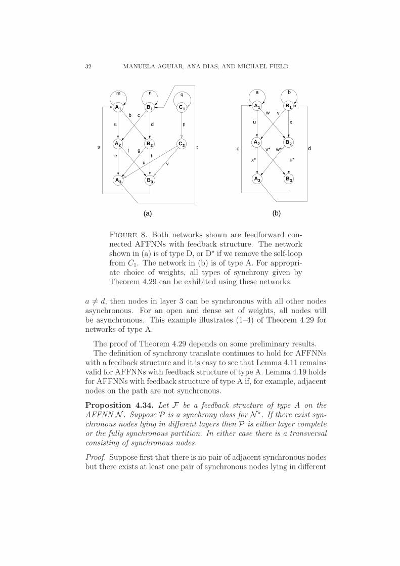
Examples 4.33. In Figure 8 we show two examples of AFFNNs withfeedback. Network (a) is of type D, network (b) is of type A.(a) If a+c = b+d, e+g = f+h, s = t, m = n, u = v and p = q, then thenode pairs A1, B1, A2, B2, A3, B3 and C1, C2 may all be synchronousand ND has nodes C1, C2, connection C1→C2 and self-loop on C1. Ifthe local valencies are all equal, then all nodes may be synchronous.Otherwise, the only synchrony across layers is that between C1 andC2. For an open and dense set of weights, all nodes are asynchronous.If we remove the self-loop from C1, then the network is of type D⋆.In this case, we still can have the node pairs A1, B1, A2, B2, A3, B3

synchronous but C1, C2 cannot be synchronous and all nodes cannotbe synchronous. This example illustrates parts (3–5) of Theorem 4.29.(b) If a = w = w⋆, b = v = v⋆, c = x = x⋆, d = u = u⋆, then{{A1, B2, A3}, {B1, A2, B3}} is a layer complete synchrony partition.If the valencies are constant on layers but differ between layers, then{{Ai, Bi} | i ∈ 3} will be a synchrony class and nodes can be onlysynchronous if they are in the same layer. If x⋆ = v⋆, u⋆ = w⋆, u 6= w,


A1

A2

A3 B3

B1

B2

u

c

w v

x

dw*

x* u*

v*

a b

A1

A2

A3 B3

C2

C1B1

B2

a d

cb

ge h

u v

t

p

fs

qm n

(a) (b)

Figure 8. Both networks shown are feedforward con-nected AFFNNs with feedback structure. The networkshown in (a) is of type D, or D⋆ if we remove the self-loopfrom C1. The network in (b) is of type A. For appropri-ate choice of weights, all types of synchrony given byTheorem 4.29 can be exhibited using these networks.

a 6= d, then nodes in layer 3 can be synchronous with all other nodesasynchronous. For an open and dense set of weights, all nodes willbe asynchronous. This example illustrates (1–4) of Theorem 4.29 fornetworks of type A.

The proof of Theorem 4.29 depends on some preliminary results.The definition of synchrony translate continues to hold for AFFNNs

with a feedback structure and it is easy to see that Lemma 4.11 remainsvalid for AFFNNs with feedback structure of type A. Lemma 4.19 holdsfor AFFNNs with feedback structure of type A if, for example, adjacentnodes on the path are not synchronous.

Proposition 4.34. Let F be a feedback structure of type A on theAFFNN N . Suppose P is a synchrony class for N ⋆. If there exist syn-chronous nodes lying in different layers then P is either layer completeor the fully synchronous partition. In either case there is a transversalconsisting of synchronous nodes.

Proof. Suppose first that there is no pair of adjacent synchronous nodesbut there exists at least one pair of synchronous nodes lying in different


layers. Lemma 4.19(1) applies and we may follow the proof of Propo-sition 4.23 to obtain an integer d ∈ [1, ℓ − 1], d|ℓ, such that P is layerd-periodic. Let i ∈ L1 have a self-loop (at least one such node existssince N is an AFFNN). It follows by d-periodicity that there is a nodej ∈ Ld+1 which is synchronous to i. Since i ∈ L1 has a self-loop, theremust be a node i′ ∈ Ld which is synchronous with j and adjacent to j.Contradiction.It follows that if there exists a pair of synchronous nodes lying in

different layers, then there must exist a pair i, j of adjacent synchronousnodes lying in adjacent layers. Suppose that i→j and i ∈ Lt, j ∈ Lt+1,where t ∈ [1, ℓ] (t+ 1 is computed mod ℓ). By backward iteration, weobtain a path of adjacent synchronous nodes i1→ . . .→it = i→it+1 = jand so a synchronous transversal if t ∈ {ℓ − 1, ℓ}. Suppose we cannotfind adjacent i, j with t ∈ {ℓ−1, ℓ}. Let T ∈ [2, ℓ−2] be the maximumvalue of t for which there exists an adjacent pair of i, j of synchronousnodes with i ∈ Lt, j ∈ Lt+1. By Lemma 4.11, we may choose apath τ : j→ . . .→i of length L = ℓ − 1, mod ℓ. By our maximalityassumption, τ will contain no pairs a, b of adjacent synchronous nodeswith a ∈ Ls, b ∈ Ls+1, s ∈ [T+1, ℓ]. It follows that Lemma 4.19 appliesto give a synchrony translate j′1→ . . .→j′L = j of τ . Hence there existsj′ = j′1 ∈ LT+2 which is synchronous to j. Therefore, by synchrony,there exists i′ ∈ LT+1 which is synchronous to j′ and adjacent to j′,contradicting the maximality of T .Our arguments show that if there exist synchronous nodes lying in

different layers there is a transversal consisting of synchronous nodes.Now apply the argument of Proposition 4.20 to deduce that P is eitherlayer complete or the fully synchronous partition. �

Lemma 4.35. Let F be a feedback structure on the AFFNN N of typeD or D⋆ and P be a synchrony class for N ⋆.

(1) If N ⋆ is of type D and there is a node in N ⋆A synchronous with

a node in ND, then all nodes are synchronous: P = {k}.(2) If N ⋆ is of type D⋆, it is not possible for a node in N ⋆

A to besynchronous with a node in ND.

Proof. Suppose i ∈ N ⋆A and j ∈ ND are synchronous. Choose a closed

path γ : i = i0→i1→ . . .→iL = i which necessarily is contained inN ⋆

A since the nodes in layer 1 of ND can only have a self-loop butno feedback loop. Since j is synchronous with i, we can lift the finalsegment of γ to a path τ = jp→ . . .→j0 = s where jr ∈ ND and issynchronous with iL−r, 0 ≤ r ≤ p, and jp ∈ L1. Either jp has no self-loop—contradicting the synchrony of jp and iL−p or jp has a self loop.In the latter case all the nodes i0, . . . , iL−p all receive inputs but only


from nodes synchronous to i. Hence γ consists of nodes synchronousto i. Since γ contains a transversal of synchronous nodes, it followseasily by feedforward connectedness that P = {k}. In particular, N ⋆

is of type D since a network of type D⋆ has a node with no input. �

Lemma 4.36. Let F be a feedback structure on the AFFNN N of typeD or D⋆ and P be a synchrony class for N ⋆. If there is a pair ofsynchronous nodes in N ⋆

A lying in different layers, then P = {k} andF is of type D.

Proof. From Proposition 4.34 we have that the synchrony class forN ⋆

A is either layer complete or the fully synchronous partition. FromLemma 4.25(1) we have that the number of layers of ND (or N ⋆

D) is lessthan ℓ. It follows that there are at least two synchronous nodes i, j inN ⋆

A such that one receives an input from a node d in ND (or N ⋆D) and

the other does not receive any input from ND (or N ⋆D). Thus d must

be synchronous with i, j. The result follows by Lemma 4.35. �

Proof of Theorem 4.29. Statement (1) follows from Proposition 4.34.Statement (2) is obvious since a network of type D⋆ always containsa pair of asynchronous nodes. Statement (3) is clear since given theadjacency matrix, it is possible (and easy) to choose weights so thatall nodes are asynchronous. Statement (5) follows from Lemmas 4.35,4.36 and this leaves (4) as the only other possibility. �

4.5. {2, . . . , ℓ − 1}-feedback structures on (A)FFNNs. We givetwo results on {2, . . . , ℓ− 1}-feedback structures. The straightforwardproofs use ideas from [1, Theorem 3.4 & Lemmas 4.7, 4.8] and areomitted.

Proposition 4.37. If N is an FFNN with a {2, . . . , ℓ − 1}-feedbackstructure with synchrony partition {Pa}a∈s, then each Pa is containedin a single layer: nodes in different layers are not synchronous.

Proposition 4.38. Let N be an AFFNN with a {2, . . . , ℓ−1}-feedbackstructure with synchrony partition {Pa}a∈s. Along any transversal,there are the following possibilities:

(1) All nodes are synchronous.(2) An initial segment of the transversal is synchronous, the re-

maining nodes are asynchronous.(3) All nodes are asynchronous.

5. Concluding remarks

Definitions for weight dynamics and examples of adaptation rulesrespecting synchrony were given in Section 3. All of this applies to


feedforward networks with feedback. However, our interest lies ratherin allowing the weights on a feedforward network to evolve to their finalstable state—if that exists—and then investigating how the addition offixed feedback loops can affect dynamics and structure of the resultingnetwork. In particular, quantifying bifurcations that can occur whenfeedback is added, and understanding the extent to which a judiciouschoice of feedback can optimize the function of the network [4, 5, 6](this is the subject of [2]). Already, in Section 4, we have seen how theaddition of feedback can enrich the possible synchrony that occur in thenetwork. In terms of unsupervised learning, this suggests enhancementof the potential for unsupervised learning even in a context where wedo not add inhibition to layers of the network.

References

[1] M A D Aguiar, A Dias, & F Ferreira. ‘Patterns of synchrony for feed-forwardand auto-regulation feed-forward neural networks’, Chaos 27 (2017) 013103.

[2] M A D Aguiar, A Dias, & M J Field. ‘Bifurcation, dynamics and feedback foradaptive feed-forward networks’, in preparation.

[3] P Ashwin and A Rodrigues. ‘Hopf normal form with SN symmetry and reduc-tion to systems of nonlinearly coupled phase oscillators’, Physica D: Nonlinear

Phenomena 325 (2016), 14–24.[4] C Bick and M J Field. ‘Asynchronous Networks and Event Driven Dynamics’,

Nonlinearity 30(2) (2017), 558–594.[5] C Bick and M J Field. ‘Asynchronous Networks: Modularization of Dynamics

Theorem’, Nonlinearity 30(2) (2017), 595–621.[6] C Bick and M J Field. ‘Functional Asynchronous Networks: Factorization of

Dynamics and Function’, (MATEC Web of Conferences, 83 (2016), CSNDD2016 - International Conference on Structural Nonlinear Dynamics and Diag-nosis, Marrakech, May 23–25, 2016).

[7] C M Bishop. Neural Networks for Pattern Recognition. (Oxford: Oxford Uni-versity Press, 1995).

[8] N Caporale and Y Dan. ‘Spike timing dependent plasticity: a Hebbian learningrule’ Annu. Rev. Neurosci. 31 (2008), 25–36.

[9] S Chandra, D Hathcock, K Crain, T M Antonsen, M Girvan, and E Ott.‘Modeling the network dynamics of pulse-coupled neurons’, Chaos 27 (2017).

[10] B. A. Davey and H. A. Priestley. Introduction to Lattices and Order (Cam-bridge University Press, 1990).

[11] G B Ermentrout and N Kopell. ‘Parabolic bursting in an excitable systemcoupled with a slow oscillation,’ SIAM J. Appl. Math. 46 (1986), 233-253.

[12] M J Field. ‘Heteroclinic Networks in Homogeneous and Heterogeneous Identi-cal Cell Systems’, J. Nonlinear Science 25(3) (2015), 779–813.

[13] W Gerstner, R Kempter, L J van Hemmen & H Wagner. ‘A neuronal learningrule for sub-millisecond temporal coding’, Nature 383 (1996), 76–78.

[14] S Goedeke and M Diesmann. ‘The mechanism of synchronization in feed-forward neuronal networks’, New J. Phys. 10 (2008).


[15] M Golubitsky and I Stewart. ‘Nonlinear dynamics of networks: the groupoidformalism’. Bull. Amer. Math. Soc. 43 (2006), 305–364.

[16] M Golubitsky, I Stewart, & A. Torok. ‘Patterns of synchrony in coupled cellnetworks with multiple arrows’, SIAM J. on Appl. Dyn. Sys. 4(1) (2005), 78–100.

[17] I Goodfellow, Y Bengio, and A Courville. Deep Learning (MIT Press, 2017).[18] B Hadley. Pattern Recognition and Neural Networks (Cambridge University

Press, 2007).[19] M H Hassoun. Fundamentals of Artificial Neural Networks (MIT Press, Cam-

bridge Mass. 1995).[20] F C Hoppensteadt and E M Izhikevich. Weakly Connected Neural Networks

(Applied Mathematical Science vol. 126, Berlin: Springer, 1997).[21] J Ito and K Kaneko. ‘Self-organized hierarchical structure in a plastic network

of chaotic units’, Neural Networks 13(3) (2000), 275–281.[22] J Ito and K Kaneko. ‘Spontaneous Structure Formation in a Network of

Chaotic Units with Variable Connection Strengths’, Phys. Rev. Lett 88(2)(2002),

[23] K Kaneko. ‘Relevance of dynamical clustering to biological networks’, PhysicaD 75 (1994), 55–73.

[24] Y Kuramoto. Chemical Oscillations, Waves, and Turbulence (Berlin: Springer,1984).

[25] H L Lee, V Padmanabhan, & S Whang. ‘Information Distortion in a SupplyChain: The Bullwhip Effect’, Management Science 43(4) (1997), 546–558.

[26] K K Lin, E Shea-Brown, & L-S Young. ‘Spike-Time Reliability of LayeredNeural Oscillator Networks’, J. Comp. Neurosci. 27 (2009), 135–160.

[27] T Masquelier, R Guyonneau, & S J Thorpe. ‘Spike Timing Dependent Plastic-ity Finds the Start of Repeating Patterns in Continuous Spike Trains’, PLoSONE 3(1) (2008), e1377.

[28] T Masquelier, R Guyonneau, & S J Thorpe. ‘Competitive STDP-Based SpikePattern Learning’, Neural Computation 21(5) (2009), 1259–1276

[29] T Masquelier, E Hugues, G Deco & S J Thorpe. ‘Oscillations, Phase-of-Firing-Coding, and Spike Timing-Dependent Plasticity: An Efficieint LearningScheme’, J. of Neuroscience 29(43) (2009), 13484–13493.

[30] M Minsky and S Papert. Perceptrons: An introduction to Computational Ge-

ometry (MIT press, 1969).[31] A Morrison, M Diesmann, & W Gerstner. ‘Phenomenological models of synap-

tic plasticity based on spike timing’, Biol. Cybern. (2008), 459-478.[32] Pedantic of Purley. ‘Uncircling the Circle: Part I’. (On line article

https://www.londonreconnections.com/2013/uncircling-circle-part-1/, in Lon-

don Reconnections, October 3, 2013.)[33] F Rosenblatt. ‘The Perceptron: A Probabilistic Model For Information Storage

And Organization In The Brain’. Psych. Rev. 65(6) (1958), 386–408.[34] P Sailamul, J Jang, & S-B Paik. ‘Synaptic convergence regulates

synchronization-dependent spike transfer in feedforward neural networks’, J.Comput. Neurosci. 43 (2017), 189–202.

[35] J Schmidhuber. ‘Deep Learning in Neural Networks: An Overview’. NeuralNetworks 61 (2015), 85-117.


[36] I Stewart. ‘The lattice of balanced equivalence relations of a coupled cell net-work’, Math. Proc. Cambridge Philos. Soc. 143 (1) (2007), 165–183.

[37] I Stewart, M Golubitsky, & M. Pivato. ‘Symmetry groupoids and patterns ofsynchrony in coupled cell networks’, SIAM J. on Appl. Dyn. Sys. 2(4) (2003),609–646.

[38] F Takens. Detecting strange attractors in turbulence (Lecture Notes in Math-ematics 898, Berlin:Springer-Verlag, 1981).

Manuela Aguiar, Faculdade de Economia, Centro de Matematica,

Universidade do Porto, Rua Dr Roberto Frias, 4200-464 Porto, Por-

tugal.

E-mail address : [email protected]

Ana Dias, Departamento de Matematica, Centro de Matematica,

Universidade do Porto, Rua do Campo Alegre, 687, 4169-007 Porto,

Portugal


Michael Field, Department of Mathematics, Imperial College, South

Kensington Campus, London SW7 2AZ, UK


FEEDFORWARD NETWORKS: ADAPTATION, …mrasmuss/preprints/DynamIC_2018_4.pdf · FEEDFORWARD NETWORKS:...

Documents

Transcript of FEEDFORWARD NETWORKS: ADAPTATION, …mrasmuss/preprints/DynamIC_2018_4.pdf · FEEDFORWARD NETWORKS:...