FEEDFORWARD NETWORKS: ADAPTATION, FEEDBACK, AND SYNCHRONY · FEEDFORWARD NETWORKS: ADAPTATION,...
66
FEEDFORWARD NETWORKS: ADAPTATION, FEEDBACK, AND SYNCHRONY MANUELA AGUIAR, ANA DIAS, AND MICHAEL FIELD Abstract. We investigate the effect on synchrony of adding feed- back loops and adaptation to a large class of feedforward networks. We obtain relatively complete results on synchrony for identical cell networks with additive input structure and feedback from the final to the initial layer of the network. These results extend previous work on synchrony in feedforward networks by Aguiar, Dias and Ferreira [2]. We also describe additive and multiplicative adapta- tion schemes that are synchrony preserving and briefly comment on dynamical protocols for running the feedforward network that relate to unsupervised learning in neural nets and neuroscience. Contents 1. Introduction 2 1.1. Background on feedforward networks 3 1.2. Dynamical feedforward networks 7 1.3. Objectives and Motivation 9 1.4. Examples: Dynamics, Synchrony and Bifurcation 11 1.5. Main results and outline of paper 21 2. A class of networks with additive input structure 22 2.1. Weighted networks 22 2.2. Synchrony subspaces 24 Date : September 29, 2018. 1
Transcript of FEEDFORWARD NETWORKS: ADAPTATION, FEEDBACK, AND SYNCHRONY · FEEDFORWARD NETWORKS: ADAPTATION,...
FEEDFORWARD NETWORKS: ADAPTATION,FEEDBACK, AND SYNCHRONY
MANUELA AGUIAR, ANA DIAS, AND MICHAEL FIELD
Abstract. We investigate the effect on synchrony of adding feed-
back loops and adaptation to a large class of feedforward networks.
We obtain relatively complete results on synchrony for identical cell
networks with additive input structure and feedback from the final
to the initial layer of the network. These results extend previous
work on synchrony in feedforward networks by Aguiar, Dias and
Ferreira [2]. We also describe additive and multiplicative adapta-
tion schemes that are synchrony preserving and briefly comment
on dynamical protocols for running the feedforward network that
relate to unsupervised learning in neural nets and neuroscience.
Contents
1. Introduction 2
1.1. Background on feedforward networks 3
1.2. Dynamical feedforward networks 7
1.3. Objectives and Motivation 9
1.4. Examples: Dynamics, Synchrony and Bifurcation 11
1.5. Main results and outline of paper 21
2. A class of networks with additive input structure 22
2.1. Weighted networks 22
2.2. Synchrony subspaces 24
Date: September 29, 2018.1
2 MANUELA AGUIAR, ANA DIAS, AND MICHAEL FIELD
3. Adaptation and Weight Dynamics 27
4. Network compatibility 31
4.1. Network compatibility partition 32
5. Layered structure and feed forward networks 39
5.1. Notation and assumptions 40
5.2. Feedback structures on an (A)FFNN 40
5.3. Adaptation on feed forward networks 43
6. Synchrony for FFNNs with feedback structure. 43
7. Synchrony for AFFNNs with feedback structure 51
8. Concluding remarks 61
9. Acknowledgments 62
References 62
1. Introduction
In this paper, and its companion [3], we study the effect of adding
feedback loops to adaptive feedforward networks. Specifically, the im-
plications for synchrony, dynamics, and bifurcation. The theoretical
results in this article will focus on synchrony and be mainly algebraic
(combinatorial) in character. Although we present a few results and
examples on bifurcation and dynamics from [3] in this introduction,
the theoretical development is left to the companion article.
Aside from reviewing background on feedforward networks—mainly
coming from neural nets and learning in neuroscience—our aim in the
introduction is to describe our approach and give several motivational
FEEDFORWARD NETWORKS 3
examples that hint at some of the rich and tractable dynamical struc-
ture present in the setting of feedforward networks with feedback. We
also compare and contrast our work with prior work on synchrony (for
example, [6, 29, 1, 2]) and asynchronous networks [7, 8].
1.1. Background on feedforward networks. Dynamicists typically
regard a network of dynamical systems as modelled by a graph with
vertices or nodes representing individual dynamical systems, and edges
(usually directed) codifying interactions between nodes. Usually, evolu-
tion is governed by a system of ordinary differential equations (ODEs)
with each variable tied to a node of the graph. Examples include the
ubiquitous Kuramoto phase oscillator network, which models weak cou-
pling between nonlinear oscillators [31, 26], and coupled cell systems
as formalized by Golubitsky, Stewart et al. [46, 22, 21].
Feedforward networks play a well-known and important role in net-
work theory and appear in many applications ranging from synchro-
nization in feed-forward neuronal networks [18, 43], to the modelling of
learning and computation—data processing (see below). Yet feedfor-
ward networks often do not fit smoothly into the dynamicists lexicon for
networks. Feedforward networks, such as artificial neural nets (ANNs)
and network models for visualization and learning in the brain, usually
process input data sequentially and not synchronously as is the case in
a dynamical network. More precisely, a feedforward network is divided
into layers—the (hidden) layers of an ANN—and processing proceeds
layer-by-layer rather than simultaneously across all layers as happens
with networks modelled by systems of differential equations. The way
4 MANUELA AGUIAR, ANA DIAS, AND MICHAEL FIELD
in which data is processed—synchronously or sequentially—can have a
major impact on both dynamics and output (see Example 1.2 below).
An additional feature of many feedforward networks is that they have
a function, represented by going from the input layer to the output
layer. Optimization of network function typically requires the network
to be adaptive.
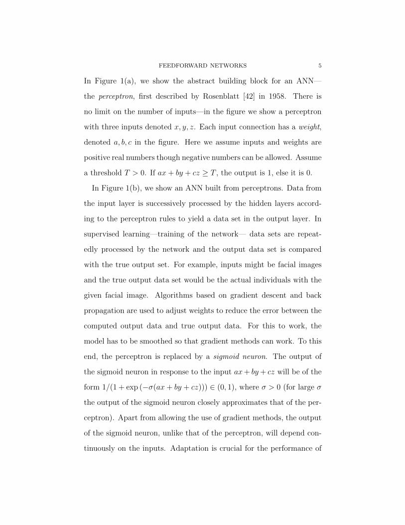
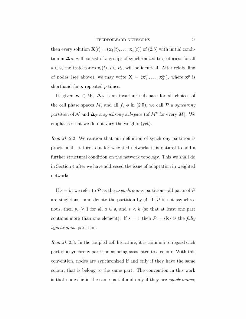
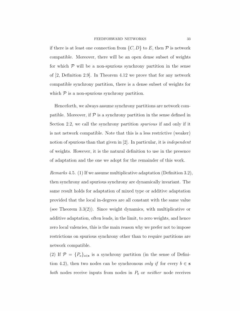
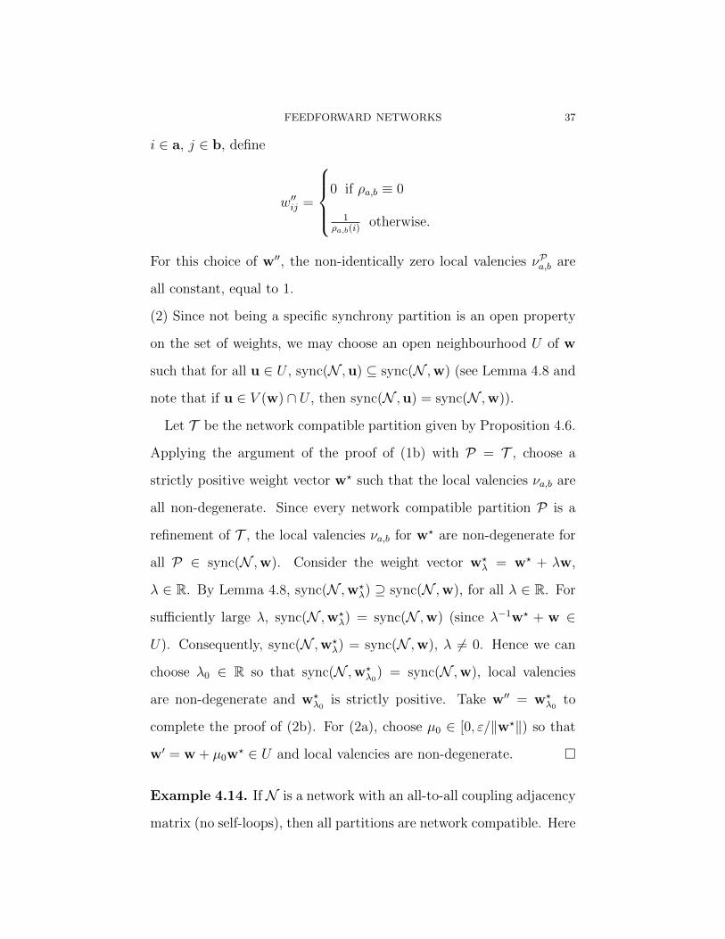
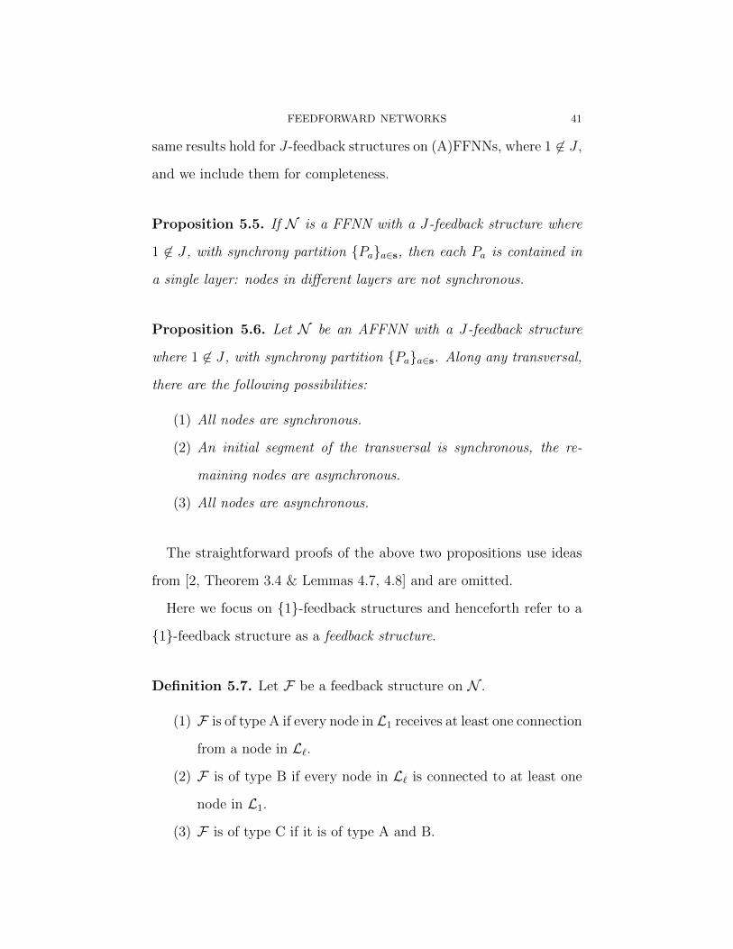
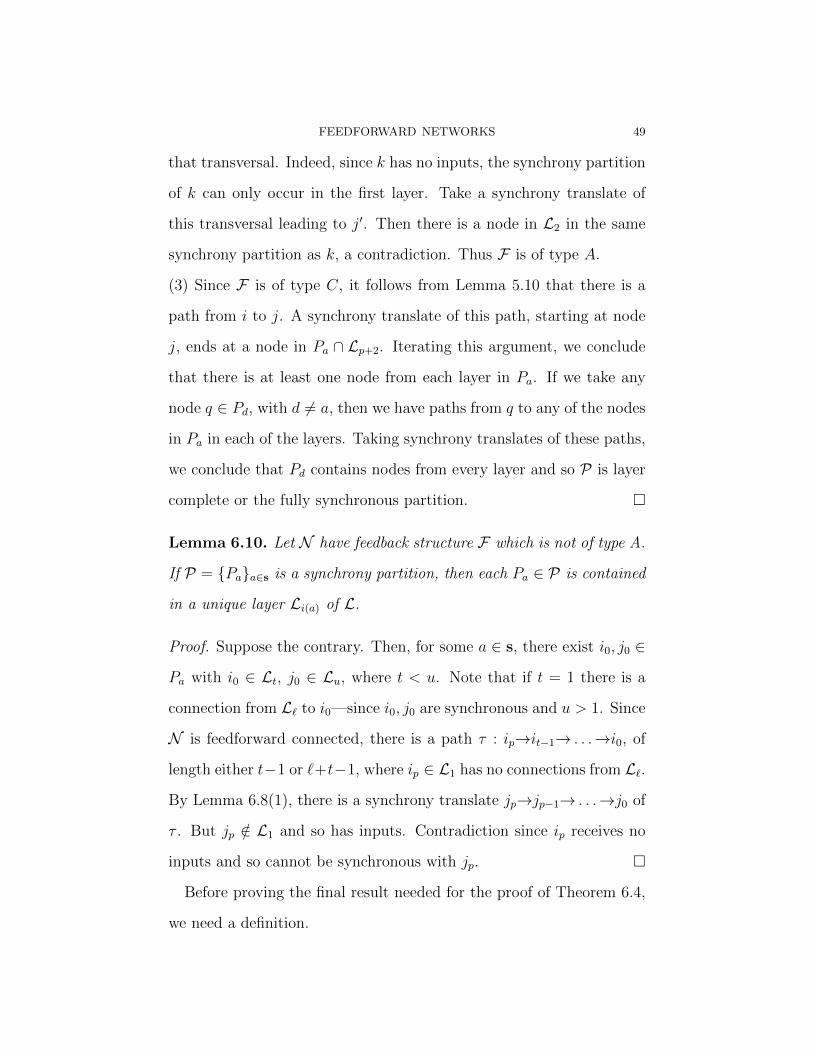
Example 1.1 (Artificial Neural Nets & Supervised Learning). The
interest in ANNs lies in their potential for approximating or represent-
ing highly complex and essentially unknown functions. For example,
a map from a large set of facial images to a set of individuals with
those facial images (facial recognition) or from a large set of drawn or
printed characters to the actual characters (handwriting recognition).
An approximation to the required function is obtained by a process of
training and adaptation. No attempt is made to derive an “analytic”
form for the function. We sketch only the simplest model and refer the
reader to the extensive literature for more details, greater generality
and related methods [10, 24, 25, 44, 23].
Hidden layers
Outp
ut la
yer
Input la
yer
(b)
a
b
c
z
y
x
Sigmoid Neuron
(a)
Perceptron
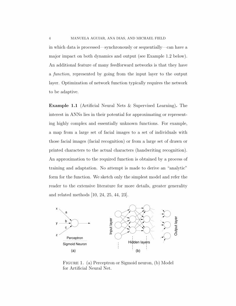
Figure 1. (a) Perceptron or Sigmoid neuron, (b) Modelfor Artificial Neural Net.
FEEDFORWARD NETWORKS 5
In Figure 1(a), we show the abstract building block for an ANN—
the perceptron, first described by Rosenblatt [42] in 1958. There is
no limit on the number of inputs—in the figure we show a perceptron
with three inputs denoted x, y, z. Each input connection has a weight,
denoted a, b, c in the figure. Here we assume inputs and weights are
positive real numbers though negative numbers can be allowed. Assume
a threshold T > 0. If ax+ by + cz ≥ T , the output is 1, else it is 0.
In Figure 1(b), we show an ANN built from perceptrons. Data from
the input layer is successively processed by the hidden layers accord-
ing to the perceptron rules to yield a data set in the output layer. In
supervised learning—training of the network— data sets are repeat-
edly processed by the network and the output data set is compared
with the true output set. For example, inputs might be facial images
and the true output data set would be the actual individuals with the
given facial image. Algorithms based on gradient descent and back
propagation are used to adjust weights to reduce the error between the
computed output data and true output data. For this to work, the
model has to be smoothed so that gradient methods can work. To this
end, the perceptron is replaced by a sigmoid neuron. The output of
the sigmoid neuron in response to the input ax+ by+ cz will be of the
form 1/(1 + exp (−σ(ax+ by + cz))) ∈ (0, 1), where σ > 0 (for large σ
the output of the sigmoid neuron closely approximates that of the per-
ceptron). Apart from allowing the use of gradient methods, the output
of the sigmoid neuron, unlike that of the perceptron, will depend con-
tinuously on the inputs. Adaptation is crucial for the performance of
6 MANUELA AGUIAR, ANA DIAS, AND MICHAEL FIELD
artificial neural networks: Minsky and Papertin showed in their 1969
book [37] that, without adaptation, ANNs based on the perceptron
could not perform some basic pattern recognition operations.
From a dynamical point of view, an ANN can be regarded as a com-
posite of maps—one for each layer—followed by a map acting on weight
space. Note that the processing is layer-by-layer and not synchronous.
In particular, an artificial neural net is not modelled by a discrete dy-
namical system—at least in the conventional sense.
The inspiration for artificial neural nets comes from neuroscience
and learning. In particular, the perceptron is a model for a spiking
neuron. The adaptation, although inspired by ideas from neuroscience
and Hebbian learning, is global in character and does not have an
obvious counterpart in neuroscience.
There does not seem to be a natural or productive way to replace the
nodes in an ANN with continuous dynamical systems—at least within
the framework of supervised learning. Indeed, the supervised learning
model attempts to construct a good approximation to a function that
acts on data sets. This is already a hard problem and it is not clear
why one would want to develop the framework to handle data sets
parametrised by time1. However, matters change when one considers
unsupervised learning. In this case there are models from neuroscience
involving synaptic plasticity, such as Spike-Timing Dependent Plastic-
ity (STDP), which involve dynamics and asynchronous or sequential
1In dynamical systems theory there are methods based on the Takens embeddingtheorem [47] that allow reconstruction of complex dynamical systems from timeseries data. However, these techniques seem not to be useful in data processing.
FEEDFORWARD NETWORKS 7
computation. In the case of STDP, learning and adaptation are con-
trolled by relative timings of spike firing (we refer to [16, 38, 11] for
more details, examples and references and note that adaptive rules for
a weight typically depend only on states of neurons at either end of the
connection—axon). It has been observed that adaptive models using
STDP are capable of pattern recognition in noisy data streams (for
example, [34, 35, 36]).
As a possible application of this viewpoint, one can envisage data
processing of a continuous data stream by an adaptive feedforward
network comprised of layers consisting of continuous dynamical units.
Here the output would reflect dynamical structure in the data stream—
for example, periodicity or quantifiable chaotic behaviour. The pro-
cessing could be viewed as a dynamic filter and the approach can be
contrasted with reconstruction techniques based on the Takens embed-
ding theorem.
1.2. Dynamical feedforward networks. We view dynamical feed-
forward networks as ‘primitive’ network objects in the sense that it is
often possible to give and/or compute a simple description of the dy-
namics by layer. Unlike what generally happens in all-to-all or strongly
connected networks, the dynamics of an individual layer in a feedfor-
ward network often has a direct and quantifiable impact on the dy-
namics of the network—reductive methods can often be used [7, §1.3].
For example, the dynamics of layer 1 is independent of the dynamics
of subsequent layers. In the simplest cases, running layer 1 (but not
8 MANUELA AGUIAR, ANA DIAS, AND MICHAEL FIELD
subsequent layers) will result in dynamics of each node in layer 1 con-
verging to an equilibrium or periodic solution. If we then switch on
the second layer then, after a transient, the dynamics on each node
will again often converge to either an equilibrium or periodic orbit. In
this way, we can evolve to a final state for the network by successively
switching on subsequent layers after the transient for the previously
layer has decayed. We call this sequential computation of dynamics (as
opposed to synchronous computation) and note the parallel with neural
nets (see Example 1.2 below for an example). In the event that each
layer evolves to an equilibrium state, we only need evolve each layer in
turn until the transient has decayed. An advantage of sequential com-
putation is that transients are not amplified through the network. This
is relevant for production and transport networks (cf. the discussion in
Bick & Field [7, §1.4]).
If we regard dynamical feedforward networks as primitive dynamical
building blocks, then it is natural to investigate the effect of adding
feedback loops to a feedforward network. The addition of a feedback
loop can sometimes be viewed as an evolutionary adaptation with the
potential to optimize a network function (see the discussions in [8, §6],
[7, §1.6]). We assume throughout that nodes have an additive input
structure—this allows for the natural addition or deletion of connec-
tions (see Section 2.1). From the structural point of view, adding a
feedback loop from the final to the first layer of a feedforward network
results in a new dynamical object and can sometimes lead to dramatic
FEEDFORWARD NETWORKS 9
bifurcation in the synchrony structure of the network as well as inter-
esting and rich dynamics as we illustrate in Examples 1.2, 1.3 below.
We remark that if we add a feedback loop from the last layer to an in-
termediate layer A (A > 1), then the resulting object can be regarded
as a concatenation of a feedforward network with A − 1 layers and a
feedforward network with feedback from the final to the initial layer
(see [8, §4] for the concatenation of functional asynchronous networks).
Similarly comments hold if we take feedback from an intermediate layer
rather than the final layer. Our focus is on feedback from the final to
the initial layer of a feedforward network so as to emphasize indecom-
posable network objects.
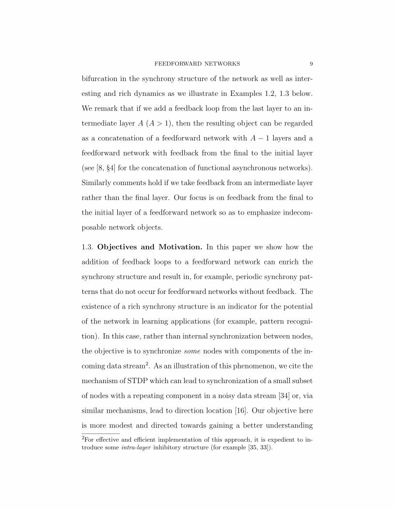
1.3. Objectives and Motivation. In this paper we show how the
addition of feedback loops to a feedforward network can enrich the
synchrony structure and result in, for example, periodic synchrony pat-
terns that do not occur for feedforward networks without feedback. The
existence of a rich synchrony structure is an indicator for the potential
of the network in learning applications (for example, pattern recogni-
tion). In this case, rather than internal synchronization between nodes,
the objective is to synchronize some nodes with components of the in-
coming data stream2. As an illustration of this phenomenon, we cite the
mechanism of STDP which can lead to synchronization of a small subset
of nodes with a repeating component in a noisy data stream [34] or, via
similar mechanisms, lead to direction location [16]. Our objective here
is more modest and directed towards gaining a better understanding
2For effective and efficient implementation of this approach, it is expedient to in-troduce some intra-layer inhibitory structure (for example [35, 33]).
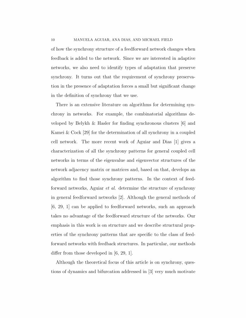
10 MANUELA AGUIAR, ANA DIAS, AND MICHAEL FIELD
of how the synchrony structure of a feedforward network changes when
feedback is added to the network. Since we are interested in adaptive
networks, we also need to identify types of adaptation that preserve
synchrony. It turns out that the requirement of synchrony preserva-
tion in the presence of adaptation forces a small but significant change
in the definition of synchrony that we use.
There is an extensive literature on algorithms for determining syn-
chrony in networks. For example, the combinatorial algorithms de-
veloped by Belykh & Hasler for finding synchronous clusters [6] and
Kamei & Cock [29] for the determination of all synchrony in a coupled
cell network. The more recent work of Aguiar and Dias [1] gives a
characterization of all the synchrony patterns for general coupled cell
networks in terms of the eigenvalue and eigenvector structures of the
network adjacency matrix or matrices and, based on that, develops an
algorithm to find those synchrony patterns. In the context of feed-
forward networks, Aguiar et al. determine the structure of synchrony
in general feedforward networks [2]. Although the general methods of
[6, 29, 1] can be applied to feedforward networks, such an approach
takes no advantage of the feedforward structure of the networks. Our
emphasis in this work is on structure and we describe structural prop-
erties of the synchrony patterns that are specific to the class of feed-
forward networks with feedback structures. In particular, our methods
differ from those developed in [6, 29, 1].
Although the theoretical focus of this article is on synchrony, ques-
tions of dynamics and bifurcation addressed in [3] very much motivate
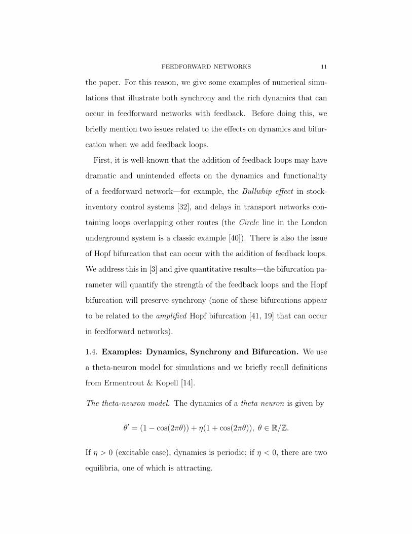
FEEDFORWARD NETWORKS 11
the paper. For this reason, we give some examples of numerical simu-
lations that illustrate both synchrony and the rich dynamics that can
occur in feedforward networks with feedback. Before doing this, we
briefly mention two issues related to the effects on dynamics and bifur-
cation when we add feedback loops.
First, it is well-known that the addition of feedback loops may have
dramatic and unintended effects on the dynamics and functionality
of a feedforward network—for example, the Bullwhip effect in stock-
inventory control systems [32], and delays in transport networks con-
taining loops overlapping other routes (the Circle line in the London
underground system is a classic example [40]). There is also the issue
of Hopf bifurcation that can occur with the addition of feedback loops.
We address this in [3] and give quantitative results—the bifurcation pa-
rameter will quantify the strength of the feedback loops and the Hopf
bifurcation will preserve synchrony (none of these bifurcations appear
to be related to the amplified Hopf bifurcation [41, 19] that can occur
in feedforward networks).
1.4. Examples: Dynamics, Synchrony and Bifurcation. We use
a theta-neuron model for simulations and we briefly recall definitions
from Ermentrout & Kopell [14].
The theta-neuron model. The dynamics of a theta neuron is given by
θ′ = (1− cos(2πθ)) + η(1 + cos(2πθ)), θ ∈ R/Z.
If η > 0 (excitable case), dynamics is periodic; if η < 0, there are two
equilibria, one of which is attracting.
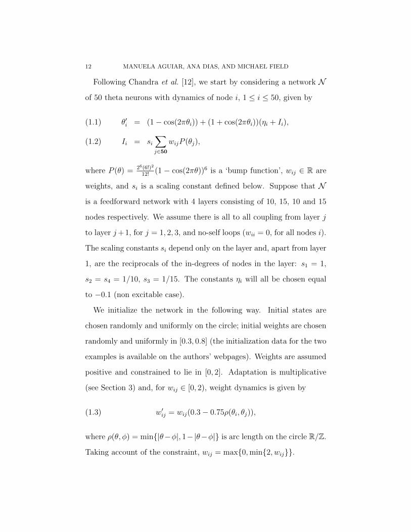
12 MANUELA AGUIAR, ANA DIAS, AND MICHAEL FIELD
Following Chandra et al. [12], we start by considering a network N
of 50 theta neurons with dynamics of node i, 1 ≤ i ≤ 50, given by
θ′i = (1− cos(2πθi)) + (1 + cos(2πθi))(ηi + Ii),(1.1)
Ii = si∑j∈50
wijP (θj),(1.2)
where P (θ) = 26(6!)2
12!(1 − cos(2πθ))6 is a ‘bump function’, wij ∈ R are
weights, and si is a scaling constant defined below. Suppose that N
is a feedforward network with 4 layers consisting of 10, 15, 10 and 15
nodes respectively. We assume there is all to all coupling from layer j
to layer j+1, for j = 1, 2, 3, and no-self loops (wii = 0, for all nodes i).
The scaling constants si depend only on the layer and, apart from layer
1, are the reciprocals of the in-degrees of nodes in the layer: s1 = 1,
s2 = s4 = 1/10, s3 = 1/15. The constants ηi will all be chosen equal
to −0.1 (non excitable case).
We initialize the network in the following way. Initial states are
chosen randomly and uniformly on the circle; initial weights are chosen
randomly and uniformly in [0.3, 0.8] (the initialization data for the two
examples is available on the authors’ webpages). Weights are assumed
positive and constrained to lie in [0, 2]. Adaptation is multiplicative
(see Section 3) and, for wij ∈ [0, 2), weight dynamics is given by
(1.3) w′ij = wij(0.3− 0.75ρ(θi, θj)),
where ρ(θ, φ) = min{|θ−φ|, 1−|θ−φ|} is arc length on the circle R/Z.
Taking account of the constraint, wij = max{0,min{2, wij}}.
FEEDFORWARD NETWORKS 13
Example 1.2 (A feedforward network of theta neurons). When the
network N is run, with or without adaptation, dynamics converges to
a fully synchronous equilibrium (individual nodes have the approximate
state 0.9025... and, with adaptation, non-zero weights all saturate at
2). This is not surprising since the individual neurons are not excitable
and the basin of attraction of the fully synchronized state is open and
dense in the phase space. All this may easily be established by direct
computation (cf. Section 1.2).
Matters become more interesting with the addition of feedback loops.
We add loops from the first node of layer 4 (node 36 of the network)
back to all nodes in layer 1. This leads to new equations
(1.4) θ′i = (1− cos(2πθi))− (0.1 + 5.7P (θ36))(1 + cos(2πθi)), i ∈ 10,
for nodes in layer 1 (we continue to assume the constants ηi = −0.1).
The weight −5.7 is fixed in what follows and is not subject to adapta-
tion.
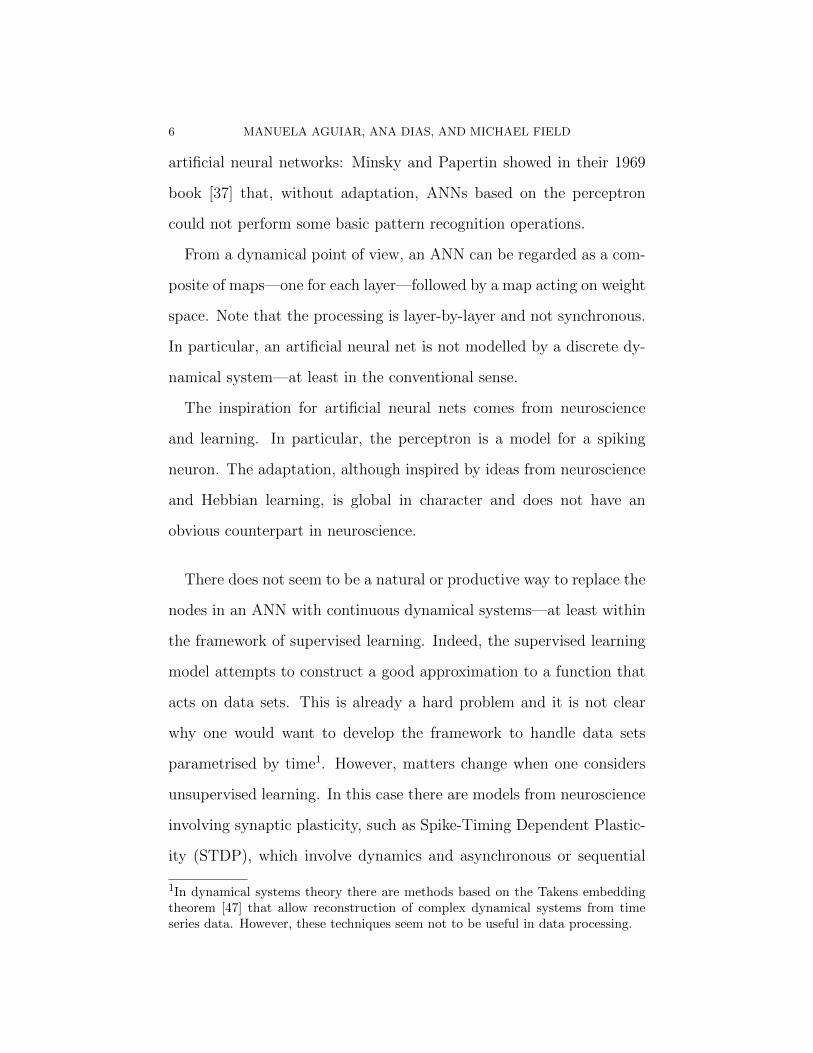
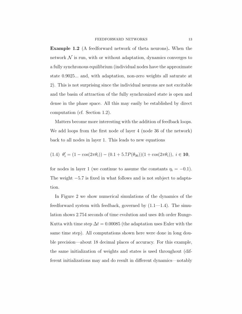
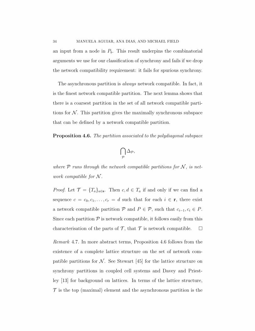
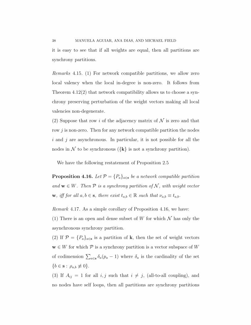
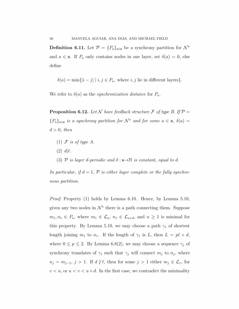
In Figure 2 we show numerical simulations of the dynamics of the
feedforward system with feedback, governed by (1.1—1.4). The simu-
lation shows 2.754 seconds of time evolution and uses 4th order Runge-
Kutta with time step ∆t = 0.00085 (the adaptation uses Euler with the
same time step). All computations shown here were done in long dou-
ble precision—about 18 decimal places of accuracy. For this example,
the same initialization of weights and states is used throughout (dif-
ferent initializations may and do result in different dynamics—notably
14 MANUELA AGUIAR, ANA DIAS, AND MICHAEL FIELD
Figure 2. Dynamics in an adaptive 50 node feedfor-ward network with 4 layers and feedback. (a) Networkdynamics: showing the dynamics of all nodes. (b) Dy-namics of nodes in layer 1. (c) Dynamics of nodes inlayer 4. For each panel, we show 2.754 seconds of timeevolution using fourth order Runge-Kutta with ∆t =0.00085.
convergence to a fully synchronous equilibrium, as in the case without
feedback).
In Figure 2(a), we show dynamics for the complete network (with
adaptation governed by (1.3)). Figure 2(b) shows the appearance of a
threshold oscillation in layer 1 after about 1.7 seconds of simulation.
FEEDFORWARD NETWORKS 15
By contrast, Figure 2(c) suggests that the dynamics on layer 4 is con-
verging to a phase oscillation (similar behaviour is seen in layers 2 and
3 and is not shown).
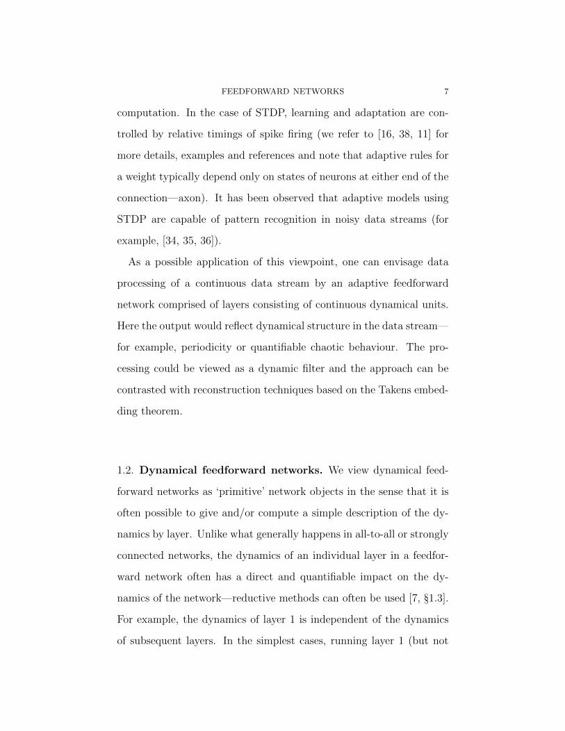
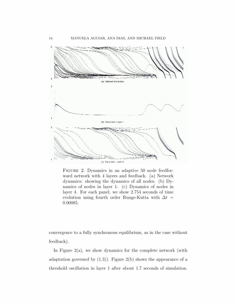
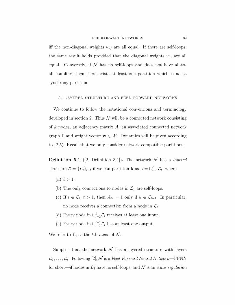
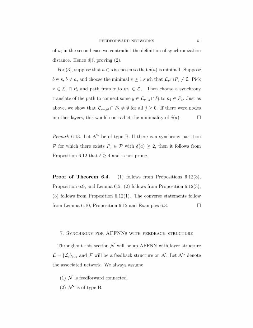
In Figure 3 we show the asymptotic behaviour of the dynamics of the
network shown in Figure 2: 1.0175 seconds of simulation are displayed
after 42.735 seconds of evolution of the network. All nodes are syn-
chronized within layers. Layers 2, 3 and 4 exhibit synchronized phase
oscillations while the nodes of layer 1 display synchronized threshold
oscillations. The oscillations are all frequency synchronized. However,
they are not phase synchronized—although the phase relationships are
periodic between layers. The oscillatory behaviour is not the result of
a Hopf bifurcation from a fully synchronous equilibrium state. Indeed,
the mechanisms leading to the appearance of the threshold oscillation—
which is very robust—appear subtle.
Choosing a different initialization of weights and states can lead
to convergence to a fully synchronous equilibrium. In every case, if
weights are all initialized to be non-zero, weights eventually all satu-
rate to the maximum allowed value of 2.0. It turns out that the fully
synchronous equilibrium and the synchronized periodic state shown in
Figure 3 are both asymptotically stable attractors. Moreover, the syn-
chronized oscillatory state has a large basin of attraction. In particular,
it is hard to perturb the oscillatory solution so that it converges to the
fully synchronous equilibrium. This is so even though most initializa-
tions of the original network (weights initialized uniformly in [0.3, 0.8])
appear to evolve to the fully synchronous equilibrium. It is natural to
16 MANUELA AGUIAR, ANA DIAS, AND MICHAEL FIELD
think of the threshold oscillation as pathological and reminiscent of the
bullwhip effect [32].
Figure 3. Periodicity and exact synchronization withinlayers for adaptive dynamics shown in Figure 2(a):1.0175 seconds of time evolution shown after 42.735 sec-onds of time evolution. Fourth order Runge-Kutta with∆t = 0.0005.
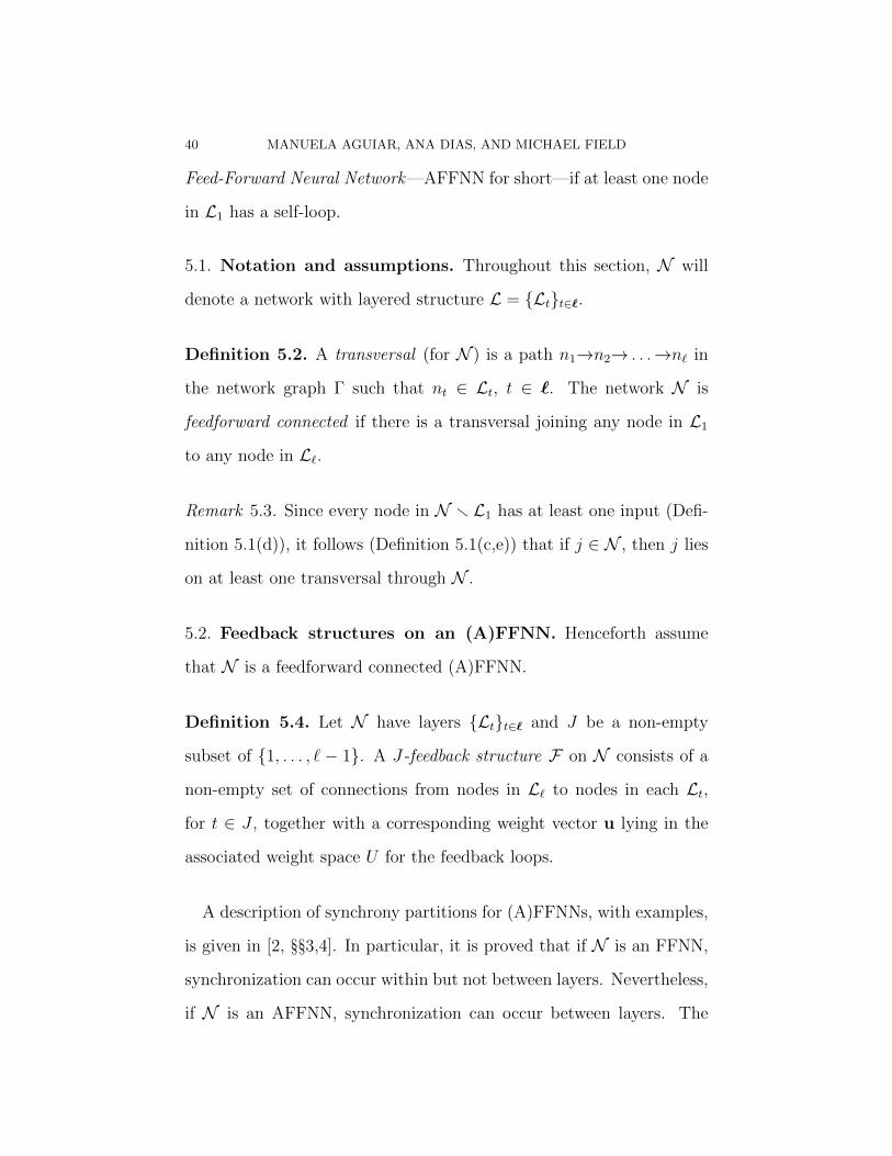
We may evolve the network using sequential computation: initially
evolve layer 1, then switch on layer 2 and evolve both layers 1 and
2, and so on until all 4 layers are evolving (synchronous computation).
We show the result for layer 1 in Figure 4 over a period of 17.09 seconds
of simulation. In this case, layer 2 is switched on after 4.27 seconds,
layer 3 after 8.54 seconds and all layers after 12.82 seconds. Until layer
4 switched on, nodes in layer 1 converge to a synchronized equilibrium
at θ = 0.564.... After layer 4 is switched on, the nodes in layer 1 start
to oscillate synchronously (as shown in Figure 2(b)) but the oscillation
decays after a few seconds and all 50 nodes converge to a fully syn-
chronous asymptotically stable equilibrium state at θ = 0.9025.... Of
course, using sequential computation avoids the propagation of large
transients through the network. Indeed, if we increase the time be-
tween switching on layers, then the oscillatory transient decays faster.
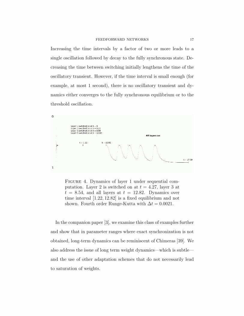
FEEDFORWARD NETWORKS 17
Increasing the time intervals by a factor of two or more leads to a
single oscillation followed by decay to the fully synchronous state. De-
creasing the time between switching initially lengthens the time of the
oscillatory transient. However, if the time interval is small enough (for
example, at most 1 second), there is no oscillatory transient and dy-
namics either converges to the fully synchronous equilibrium or to the
threshold oscillation.
Figure 4. Dynamics of layer 1 under sequential com-putation. Layer 2 is switched on at t = 4.27, layer 3 att = 8.54, and all layers at t = 12.82. Dynamics overtime interval [1.22, 12.82] is a fixed equilibrium and notshown. Fourth order Runge-Kutta with ∆t = 0.0021.
In the companion paper [3], we examine this class of examples further
and show that in parameter ranges where exact synchronization is not
obtained, long-term dynamics can be reminiscent of Chimeras [39]. We
also address the issue of long term weight dynamics—which is subtle—
and the use of other adaptation schemes that do not necessarily lead
to saturation of weights.
18 MANUELA AGUIAR, ANA DIAS, AND MICHAEL FIELD
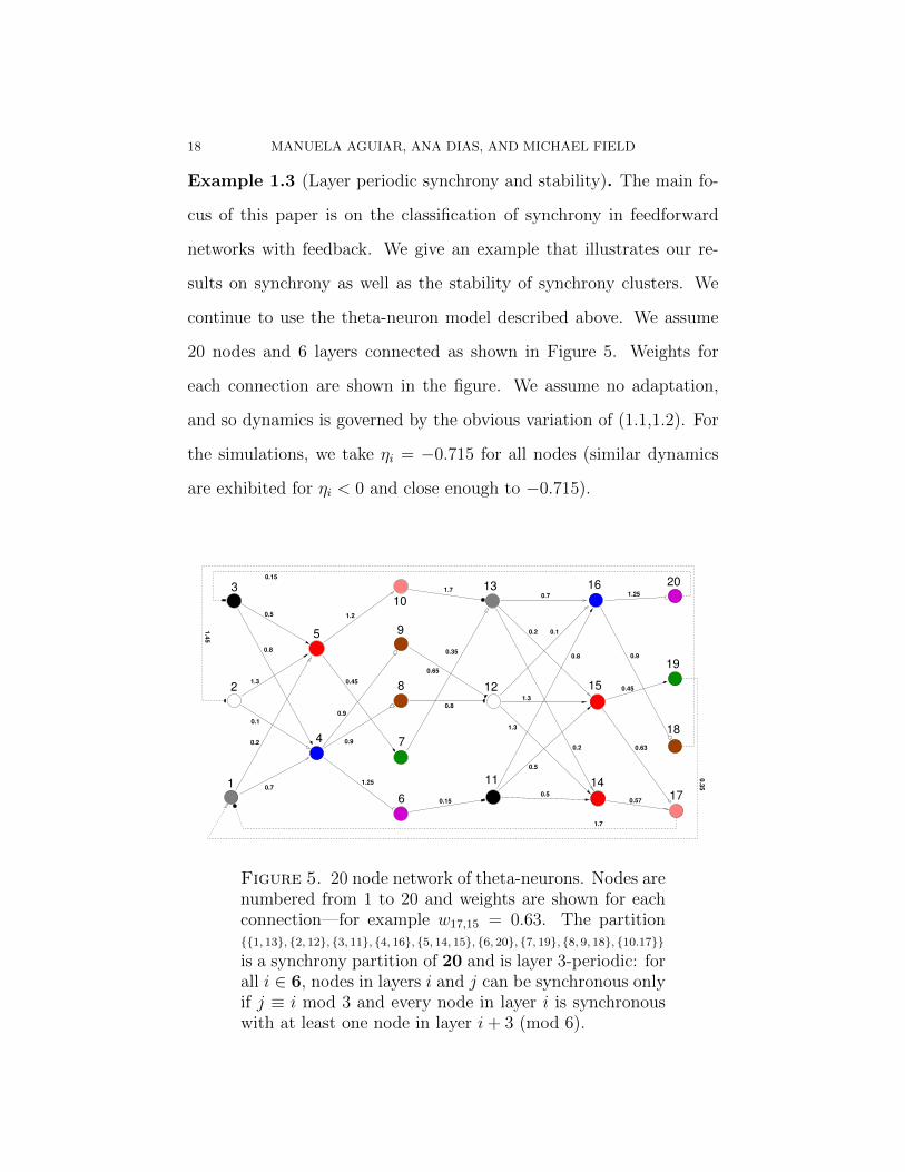
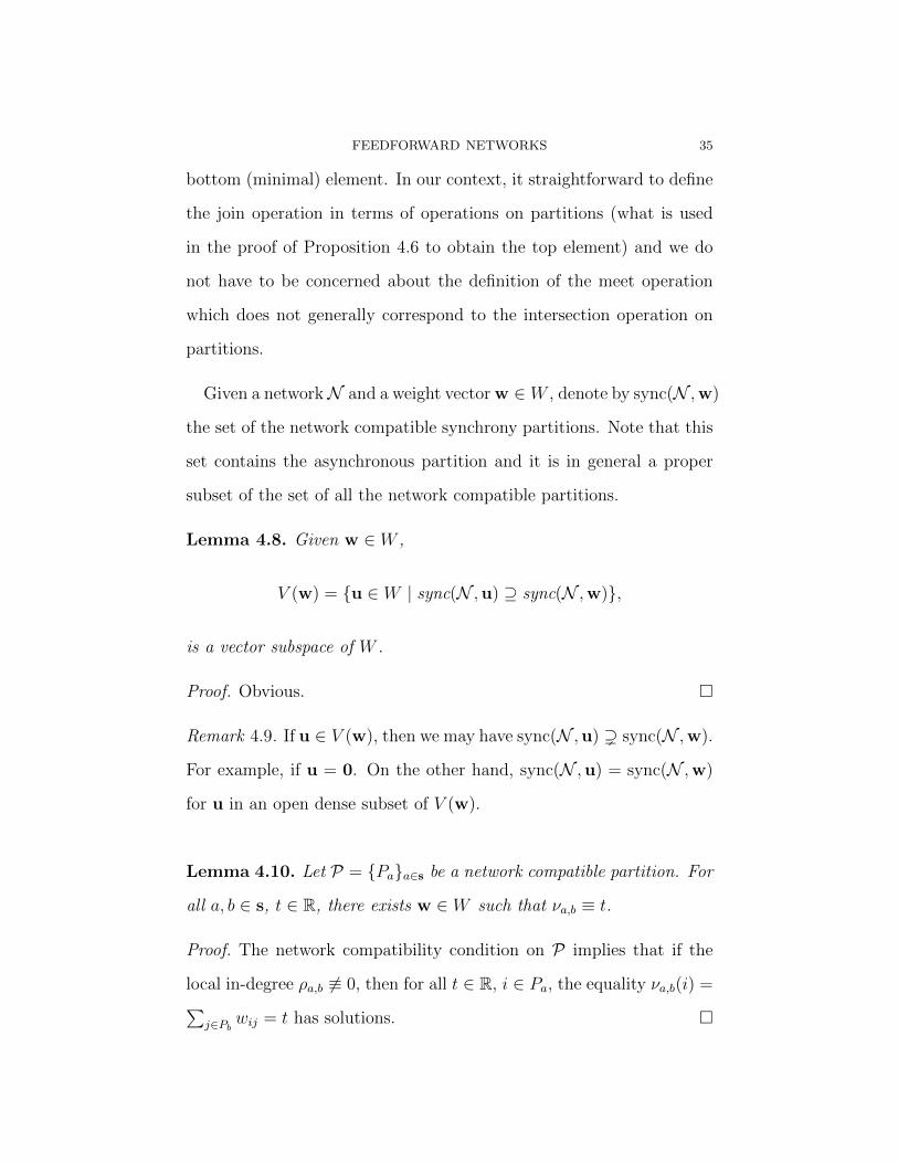
Example 1.3 (Layer periodic synchrony and stability). The main fo-
cus of this paper is on the classification of synchrony in feedforward
networks with feedback. We give an example that illustrates our re-
sults on synchrony as well as the stability of synchrony clusters. We
continue to use the theta-neuron model described above. We assume
20 nodes and 6 layers connected as shown in Figure 5. Weights for
each connection are shown in the figure. We assume no adaptation,
and so dynamics is governed by the obvious variation of (1.1,1.2). For
the simulations, we take ηi = −0.715 for all nodes (similar dynamics
are exhibited for ηi < 0 and close enough to −0.715).
1
2
3
5
4
10
9
8
7
6
12
13
11 14
15
16
17
18
19
20
1.25
1.250.7
0.2
0.2
0.2
0.9
0.9
1.2
0.5
0.5
0.45
0.45
0.63
0.57
1.3
1.3
0.8
0.8
0.1
1.3
0.5
0.7
0.15
0.15
0.9
1.4
5
1.7
1.7
0.35
0.3
5
0.1
0.65
0.8
Figure 5. 20 node network of theta-neurons. Nodes arenumbered from 1 to 20 and weights are shown for eachconnection—for example w17,15 = 0.63. The partition{{1, 13}, {2, 12}, {3, 11}, {4, 16}, {5, 14, 15}, {6, 20}, {7, 19}, {8, 9, 18}, {10.17}}
is a synchrony partition of 20 and is layer 3-periodic: forall i ∈ 6, nodes in layers i and j can be synchronous onlyif j ≡ i mod 3 and every node in layer i is synchronouswith at least one node in layer i+ 3 (mod 6).
FEEDFORWARD NETWORKS 19
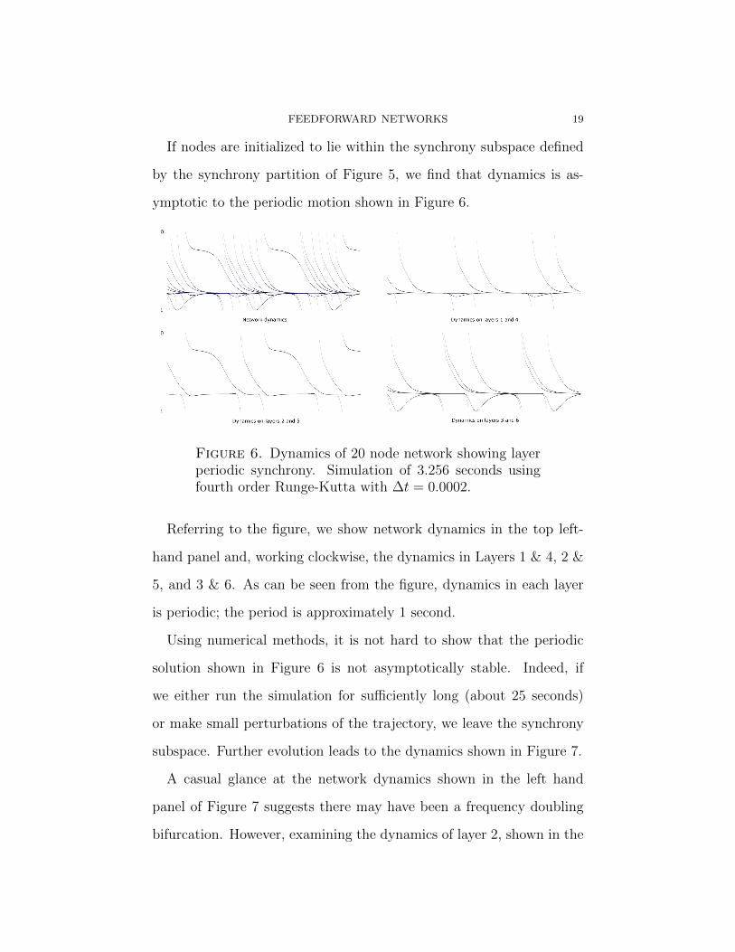
If nodes are initialized to lie within the synchrony subspace defined
by the synchrony partition of Figure 5, we find that dynamics is as-
ymptotic to the periodic motion shown in Figure 6.
Figure 6. Dynamics of 20 node network showing layerperiodic synchrony. Simulation of 3.256 seconds usingfourth order Runge-Kutta with ∆t = 0.0002.
Referring to the figure, we show network dynamics in the top left-
hand panel and, working clockwise, the dynamics in Layers 1 & 4, 2 &
5, and 3 & 6. As can be seen from the figure, dynamics in each layer
is periodic; the period is approximately 1 second.
Using numerical methods, it is not hard to show that the periodic
solution shown in Figure 6 is not asymptotically stable. Indeed, if
we either run the simulation for sufficiently long (about 25 seconds)
or make small perturbations of the trajectory, we leave the synchrony
subspace. Further evolution leads to the dynamics shown in Figure 7.
A casual glance at the network dynamics shown in the left hand
panel of Figure 7 suggests there may have been a frequency doubling
bifurcation. However, examining the dynamics of layer 2, shown in the
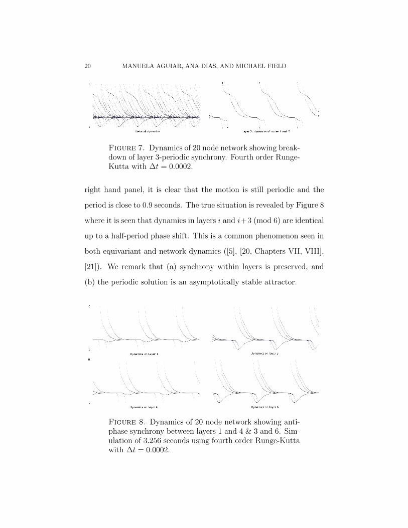
20 MANUELA AGUIAR, ANA DIAS, AND MICHAEL FIELD
Figure 7. Dynamics of 20 node network showing break-down of layer 3-periodic synchrony. Fourth order Runge-Kutta with ∆t = 0.0002.
right hand panel, it is clear that the motion is still periodic and the
period is close to 0.9 seconds. The true situation is revealed by Figure 8
where it is seen that dynamics in layers i and i+3 (mod 6) are identical
up to a half-period phase shift. This is a common phenomenon seen in
both equivariant and network dynamics ([5], [20, Chapters VII, VIII],
[21]). We remark that (a) synchrony within layers is preserved, and
(b) the periodic solution is an asymptotically stable attractor.
Figure 8. Dynamics of 20 node network showing anti-phase synchrony between layers 1 and 4 & 3 and 6. Sim-ulation of 3.256 seconds using fourth order Runge-Kuttawith ∆t = 0.0002.
FEEDFORWARD NETWORKS 21
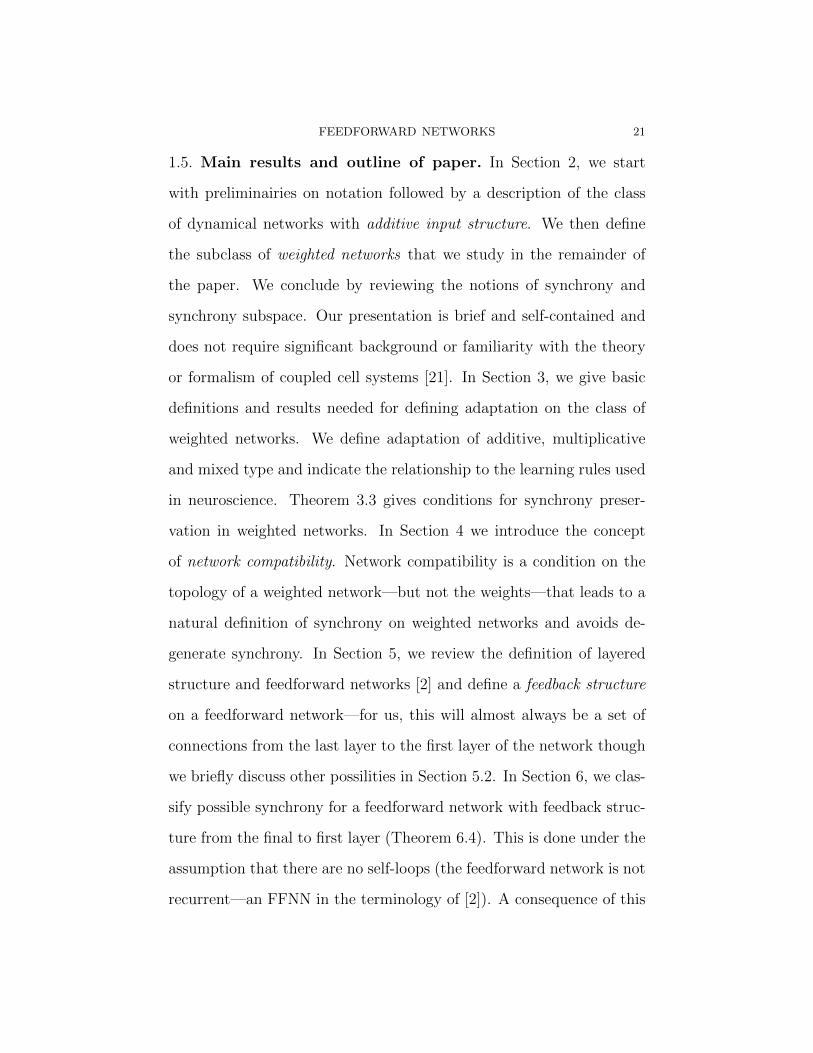
1.5. Main results and outline of paper. In Section 2, we start
with preliminairies on notation followed by a description of the class
of dynamical networks with additive input structure. We then define
the subclass of weighted networks that we study in the remainder of
the paper. We conclude by reviewing the notions of synchrony and
synchrony subspace. Our presentation is brief and self-contained and
does not require significant background or familiarity with the theory
or formalism of coupled cell systems [21]. In Section 3, we give basic
definitions and results needed for defining adaptation on the class of
weighted networks. We define adaptation of additive, multiplicative
and mixed type and indicate the relationship to the learning rules used
in neuroscience. Theorem 3.3 gives conditions for synchrony preser-
vation in weighted networks. In Section 4 we introduce the concept
of network compatibility. Network compatibility is a condition on the
topology of a weighted network—but not the weights—that leads to a
natural definition of synchrony on weighted networks and avoids de-
generate synchrony. In Section 5, we review the definition of layered
structure and feedforward networks [2] and define a feedback structure
on a feedforward network—for us, this will almost always be a set of
connections from the last layer to the first layer of the network though
we briefly discuss other possilities in Section 5.2. In Section 6, we clas-
sify possible synchrony for a feedforward network with feedback struc-
ture from the final to first layer (Theorem 6.4). This is done under the
assumption that there are no self-loops (the feedforward network is not
recurrent—an FFNN in the terminology of [2]). A consequence of this
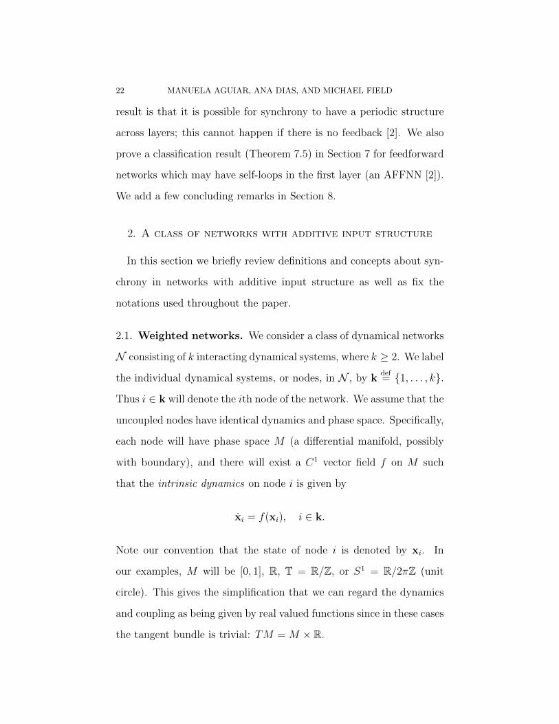
22 MANUELA AGUIAR, ANA DIAS, AND MICHAEL FIELD
result is that it is possible for synchrony to have a periodic structure
across layers; this cannot happen if there is no feedback [2]. We also
prove a classification result (Theorem 7.5) in Section 7 for feedforward
networks which may have self-loops in the first layer (an AFFNN [2]).
We add a few concluding remarks in Section 8.
2. A class of networks with additive input structure
In this section we briefly review definitions and concepts about syn-
chrony in networks with additive input structure as well as fix the
notations used throughout the paper.
2.1. Weighted networks. We consider a class of dynamical networks
N consisting of k interacting dynamical systems, where k ≥ 2. We label
the individual dynamical systems, or nodes, in N , by kdef= {1, . . . , k}.
Thus i ∈ k will denote the ith node of the network. We assume that the
uncoupled nodes have identical dynamics and phase space. Specifically,
each node will have phase space M (a differential manifold, possibly
with boundary), and there will exist a C1 vector field f on M such
that the intrinsic dynamics on node i is given by
xi = f(xi), i ∈ k.
Note our convention that the state of node i is denoted by xi. In
our examples, M will be [0, 1], R, T = R/Z, or S1 = R/2πZ (unit
circle). This gives the simplification that we can regard the dynamics
and coupling as being given by real valued functions since in these cases
the tangent bundle is trivial: TM = M × R.
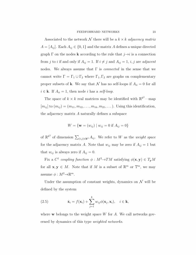
FEEDFORWARD NETWORKS 23
Associated to the network N there will be a k× k adjacency matrix
A = [Aij]. Each Aij ∈ {0, 1} and the matrix A defines a unique directed
graph Γ on the nodes k according to the rule that j→i is a connection
from j to i if and only if Aij = 1. If i 6= j and Aij = 1, i, j are adjacent
nodes. We always assume that Γ is connected in the sense that we
cannot write Γ = Γ1 ∪ Γ2 where Γ1,Γ2 are graphs on complementary
proper subsets of k. We say that N has no self-loops if Aii = 0 for all
i ∈ k. If Aii = 1, then node i has a self-loop.
The space of k × k real matrices may be identified with Rk2—map
[mij] to (mij) = (m11,m12, . . . ,m1k,m21, . . . ). Using this identification,
the adjacency matrix A naturally defines a subspace
W = {w = (wij) | wij = 0 if Aij = 0}
of Rk2 of dimension∑
(i,j)∈k2 Aij. We refer to W as the weight space
for the adjacency matrix A. Note that wij may be zero if Aij = 1 but
that wij is always zero if Aij = 0.
Fix a C1 coupling function φ : M2→TM satisfying φ(x,y) ∈ TyM
for all x,y ∈ M . Note that if M is a subset of Rm or Tm, we may
assume φ : M2→Rm.
Under the assumption of constant weights, dynamics on N will be
defined by the system
(2.5) xi = f(xi) +k∑j=1
wijφ(xj,xi), i ∈ k,
where w belongs to the weight space W for A. We call networks gov-
erned by dynamics of this type weighted networks.
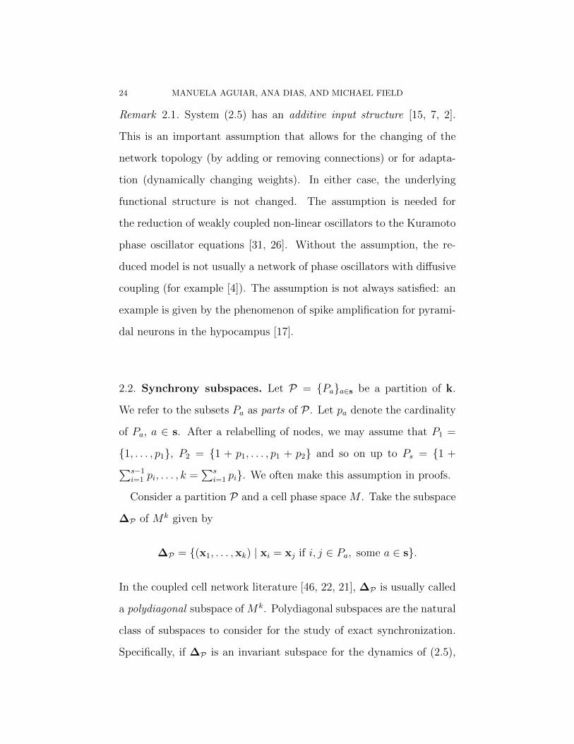
24 MANUELA AGUIAR, ANA DIAS, AND MICHAEL FIELD
Remark 2.1. System (2.5) has an additive input structure [15, 7, 2].
This is an important assumption that allows for the changing of the
network topology (by adding or removing connections) or for adapta-
tion (dynamically changing weights). In either case, the underlying
functional structure is not changed. The assumption is needed for
the reduction of weakly coupled non-linear oscillators to the Kuramoto
phase oscillator equations [31, 26]. Without the assumption, the re-
duced model is not usually a network of phase oscillators with diffusive
coupling (for example [4]). The assumption is not always satisfied: an
example is given by the phenomenon of spike amplification for pyrami-
dal neurons in the hypocampus [17].
2.2. Synchrony subspaces. Let P = {Pa}a∈s be a partition of k.
We refer to the subsets Pa as parts of P . Let pa denote the cardinality
of Pa, a ∈ s. After a relabelling of nodes, we may assume that P1 =
{1, . . . , p1}, P2 = {1 + p1, . . . , p1 + p2} and so on up to Ps = {1 +∑s−1i=1 pi, . . . , k =
∑si=1 pi}. We often make this assumption in proofs.
Consider a partition P and a cell phase space M . Take the subspace
∆P of Mk given by
∆P = {(x1, . . . ,xk) | xi = xj if i, j ∈ Pa, some a ∈ s}.
In the coupled cell network literature [46, 22, 21], ∆P is usually called
a polydiagonal subspace of Mk. Polydiagonal subspaces are the natural
class of subspaces to consider for the study of exact synchronization.
Specifically, if ∆P is an invariant subspace for the dynamics of (2.5),
FEEDFORWARD NETWORKS 25
then every solution X(t) = (x1(t), . . . ,xk(t)) of (2.5) with initial condi-
tion in ∆P , will consist of s groups of synchronized trajectories: for all
a ∈ s, the trajectories xi(t), i ∈ Pa, will be identical. After relabelling
of nodes (see above), we may write X = (xp11 , . . . ,xpss ), where xp is
shorthand for x repeated p times.
If, given w ∈ W , ∆P is an invariant subspace for all choices of
the cell phase spaces M , and all f , φ in (2.5), we call P a synchrony
partition of N and ∆P a synchrony subspace (of Mk for every M). We
emphasise that we do not vary the weights (yet).
Remark 2.2. We caution that our definition of synchrony partition is
provisional. It turns out for weighted networks it is natural to add a
further structural condition on the network topology. This we shall do
in Section 4 after we have addressed the issue of adaptation in weighted
networks.
If s = k, we refer to P as the asynchronous partition—all parts of P
are singletons—and denote the partition by A. If P is not asynchro-
nous, then pa ≥ 1 for all a ∈ s, and s < k (so that at least one part
contains more than one element). If s = 1 then P = {k} is the fully
synchronous partition.
Remark 2.3. In the coupled cell literature, it is common to regard each
part of a synchrony partition as being associated to a colour. With this
convention, nodes are synchronized if and only if they have the same
colour, that is belong to the same part. The convention in this work
is that nodes lie in the same part if and only if they are synchronous ;
26 MANUELA AGUIAR, ANA DIAS, AND MICHAEL FIELD
nodes that are not synchronous are asynchronous.
We want to give a necessary and sufficient condition for a partition
to be a synchrony partition.
Definition 2.4. Given a network N with adjacency matrix A and a
fixed weight vector W , let P = {Pa}a∈s be a partition of the network
set of cells k. For a, b ∈ s define the local valency function νa,b : Pa→R
and local in-degree function ρa,b : Pa→N by
νa,b(i) =∑j∈Pb
wij, ρa,b(i) =∑j∈Pb
Aij, i ∈ Pa.
If s = 1 set ν1,1 = ν : k→R, ρ1,1 = ρ : k→Z+0 and refer to ν and ρ as
the valency and in-degree.
The following proposition corresponds to Theorem 2.4 of [2] which is
a generalization of Theorem 6.5 of [46] to weighted networks. We use
our notation and present a different proof.
Proposition 2.5. (Notation and assumptions as above.) Given w ∈
W , P = {Pa}a∈s is a synchrony partition of N iff each local valency
function νa,b is constant.
Proof. Sufficiency. Let ta,b denote the constant value of νa,b. Consider
the network with s nodes and dynamics given by
(2.6) ya = f(ya) +∑b∈s
ta,bφ(yb,ya), a ∈ s,
FEEDFORWARD NETWORKS 27
where each node has state space M (as in (2.5)). Clearly every solution
of (2.6) determines a solution to (2.5) lying in ∆P and with initial con-
dition (yp11 (0), . . . ,ypss (0)) ∈ ∆P . It follows by uniqueness of solutions
that every solution X(t) of (2.5) with initial condition X(0) ∈ ∆P is
of this form and so X(t) ∈∆P for all t.
Necessity. Suppose that να,β is not constant for some pair (α, β) ∈ s2.
Necessarily pα > 1. It suffices to find a specific equation of the form
(2.5) for which ∆P is not an invariant subspace. For this, take M = R,
f ≡ 0. Taking xa = a, a ∈ s, choose any smooth φ : R2→R such that
φ(x, y) = 1, for (x, y) near (α, β), and φ(x, y) = 0 for values of (x, y)
near (a, b) 6= (α, β). Pick i, j ∈ Pα such that να,β(i) 6= να,β(j). Suppose
xi(0) = xj(0) = α. The equations for xi,xj near t = 0 are
xi = να,β(i), xj = να,β(j).
It follows from our assumptions on φ and choice of i, j that xi(t) 6= xj(t)
for t close to zero, t 6= 0. Hence P cannot be a synchrony partition. �
Remark 2.6. In the coupled cell literature [22, 21], a synchrony parti-
tion corresponds to a balanced equivalence relation and (2.6) are the
equations of the quotient network giving the dynamics of (2.5) on the
synchrony subspace.
3. Adaptation and Weight Dynamics
We use an adaptive scheme for weight dynamics which is natural for
the analysis of synchronization. We refer the reader to the remarks at
28 MANUELA AGUIAR, ANA DIAS, AND MICHAEL FIELD
the end of this section for connections with learning in neuroscience
and limitations on the model.
First, assume weights and dynamics evolve according to
xi = f(xi) +k∑j=1
wijφ(xj,xi), i ∈ k,(3.7)
wij = ϕ(wij,xi,xj), (i, j) ∈ N,(3.8)
where N = {(i, j) ∈ k2 | Aij = 1}, (3.7) satisfies the conditions for
(2.5), and ϕ : R×M2→R is C1. This model for dynamics and adapta-
tion assumes that the evolution of the weight wij depends only on wij
and the states of the nodes i and j.
In what follows, we assume for simplicity that solutions of (3.7,3.8)
are defined for all t ≥ 0.
Definition 3.1. Let N be a network, w ∈ W a weight vector and
dynamics for N be given by equations (3.7). The system (3.7,3.8)
preserves synchrony if for every synchrony partition P of N for the
weight w, the subspace ∆P is forward invariant by the flow of (3.7)
taking the initial condition w(0) = w for (3.8).
Of course, without further conditions, (3.7,3.8) will not preserve syn-
chrony.
Definition 3.2. (1) Adaptation is multiplicative if there is a C1
map Φ : M2→R such that
ϕ(w,x,y) = wΦ(x, y), (w, (x,y)) ∈ R×M2.
FEEDFORWARD NETWORKS 29
(2) Adaptation is additive if there is a C1 map Φ : M2→R such
that
ϕ(w,x,y) = Φ(x, y), (w, (x,y)) ∈ R×M2.
(3) Adaptation is of mixed type if there are distinct C1 maps Φ,Ψ :
M2→R and C 6= 0 such that
ϕ(w,x,y) = wΦ(x,y) + (C − w)Ψ(x,y), (w, (x,y)) ∈ R×M2.
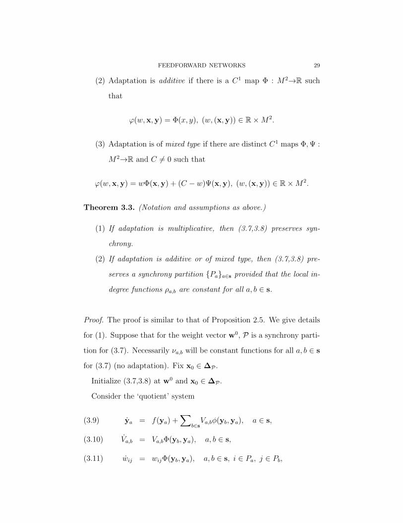
Theorem 3.3. (Notation and assumptions as above.)
(1) If adaptation is multiplicative, then (3.7,3.8) preserves syn-
chrony.
(2) If adaptation is additive or of mixed type, then (3.7,3.8) pre-
serves a synchrony partition {Pa}a∈s provided that the local in-
degree functions ρa,b are constant for all a, b ∈ s.
Proof. The proof is similar to that of Proposition 2.5. We give details
for (1). Suppose that for the weight vector w0, P is a synchrony parti-
tion for (3.7). Necessarily νa,b will be constant functions for all a, b ∈ s
for (3.7) (no adaptation). Fix x0 ∈∆P .
Initialize (3.7,3.8) at w0 and x0 ∈∆P .
Consider the ‘quotient’ system
ya = f(ya) +∑
b∈sVa,bφ(yb,ya), a ∈ s,(3.9)
Va,b = Va,bΦ(yb,ya), a, b ∈ s,(3.10)
wij = wijΦ(yb,ya), a, b ∈ s, i ∈ Pa, j ∈ Pb,(3.11)
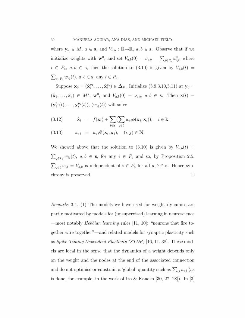
30 MANUELA AGUIAR, ANA DIAS, AND MICHAEL FIELD
where ya ∈ M , a ∈ s, and Va,b : R→R, a, b ∈ s. Observe that if we
initialize weights with w0, and set Va,b(0) = νa,b =∑
j∈Pbw0ij, where
i ∈ Pa, a, b ∈ s, then the solution to (3.10) is given by Va,b(t) =∑j∈Pb
wij(t), a, b ∈ s, any i ∈ Pa.
Suppose x0 = (xp11 , . . . , xpss ) ∈ ∆P . Initialize (3.9,3.10,3.11) at y0 =
(x1, . . . , xs) ∈ M s, w0, and Va,b(0) = νa,b, a, b ∈ s. Then x(t) =
(yp11 (t), . . . ,ypss (t)), (wij(t)) will solve
xi = f(xi) +∑b∈s
(∑j∈b
wijφ(xj,xi)), i ∈ k,(3.12)
wij = wijΦ(xi,xj), (i, j) ∈ N.(3.13)
We showed above that the solution to (3.10) is given by Va,b(t) =∑j∈Pb
wij(t), a, b ∈ s, for any i ∈ Pa and so, by Proposition 2.5,∑j∈bwij = Va,b is independent of i ∈ Pa for all a, b ∈ s. Hence syn-
chrony is preserved. �
Remarks 3.4. (1) The models we have used for weight dynamics are
partly motivated by models for (unsupervised) learning in neuroscience
—most notably Hebbian learning rules [11, 10]: “neurons that fire to-
gether wire together”—and related models for synaptic plasticity such
as Spike-Timing Dependent Plasticity (STDP) [16, 11, 38]. These mod-
els are local in the sense that the dynamics of a weight depends only
on the weight and the nodes at the end of the associated connection
and do not optimise or constrain a ‘global’ quantity such as∑
ij wij (as
is done, for example, in the work of Ito & Kaneko [30, 27, 28]). In [3]
FEEDFORWARD NETWORKS 31
we consider the dynamical implications of various choices of weight dy-
namics related to the relative timing model of STDP.
(2) In practice, it is customary to assume weights are positive and so
weight dynamics will be constrained to the positive orthant Ra+. This
is no problem for adaptation which is multiplicative or of mixed type
(with appropriate conditions). However, for additive adaptation, hard
lower and upper bounds are typically required. If weights saturate,
synchrony is usually lost. If we restrict to positive weights, then there
are no issues with spurious synchrony [2]—see also Remark 4.5 and the
discussion in Section 4.
4. Network compatibility
In a coupled identical cell network, synchrony depends only on the
network topology. In particular, synchrony is independent of the func-
tional structure of the network: synchrony measures the minimal num-
ber of synchrony subspaces that a network with given topology must
have—of course, a specific choice of network dynamics can lead to more
synchrony subspaces. As we have defined it, synchrony for weighted
networks depends on the network topology and the weights but not on
the intrinsic dynamics or coupling function (f and φ in (2.5)). As was
observed in Aguiar et al. [2], this definition is too general as it allows
for degenerate or spurious [2, Definition 2.9] synchrony partitions.
Example 4.1. Consider the network and synchrony partition P =
{{A,B}, {C,D}, {E,F}} shown in Figure 9. Following [2], P is spu-
rious: there are no connections from nodes C,D to E and the sum of
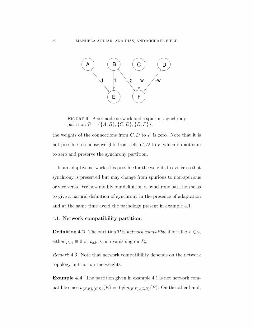
32 MANUELA AGUIAR, ANA DIAS, AND MICHAEL FIELD
1 1 2 w −w
A B C D
E F
Figure 9. A six-node network and a spurious synchronypartition P = {{A,B}, {C,D}, {E,F}}.
the weights of the connections from C,D to F is zero. Note that it is
not possible to choose weights from cells C,D to F which do not sum
to zero and preserve the synchrony partition.
In an adaptive network, it is possible for the weights to evolve so that
synchrony is preserved but may change from spurious to non-spurious
or vice versa. We now modify our definition of synchrony partition so as
to give a natural definition of synchrony in the presence of adaptation
and at the same time avoid the pathology present in example 4.1.
4.1. Network compatibility partition.
Definition 4.2. The partition P is network compatible if for all a, b ∈ s,
either ρa,b ≡ 0 or ρa,b is non-vanishing on Pa.
Remark 4.3. Note that network compatibility depends on the network
topology but not on the weights.
Example 4.4. The partition given in example 4.1 is not network com-
patible since ρ{E,F},{C,D}(E) = 0 6= ρ{E,F},{C,D}(F ). On the other hand,
FEEDFORWARD NETWORKS 33
if there is at least one connection from {C,D} to E, then P is network
compatible. Moreover, there will be an open dense subset of weights
for which P will be a non-spurious synchrony partition in the sense
of [2, Definition 2.9]. In Theorem 4.12 we prove that for any network
compatible synchrony partition, there is a dense subset of weights for
which P is a non-spurious synchrony partition.
Henceforth, we always assume synchrony partitions are network com-
patible. Moreover, if P is a synchrony partition in the sense defined in
Section 2.2, we call the synchrony partition spurious if and only if it
is not network compatible. Note that this is a less restrictive (weaker)
notion of spurious than that given in [2]. In particular, it is independent
of weights. However, it is the natural definition to use in the presence
of adaptation and the one we adopt for the remainder of this work.
Remarks 4.5. (1) If we assume multiplicative adaptation (Definition 3.2),
then synchrony and spurious synchrony are dynamically invariant. The
same result holds for adaptation of mixed type or additive adaptation
provided that the local in-degrees are all constant with the same value
(see Theorem 3.3(2)). Since weight dynamics, with multiplicative or
additive adaptation, often leads, in the limit, to zero weights, and hence
zero local valencies, this is the main reason why we prefer not to impose
restrictions on spurious synchrony other than to require partitions are
network compatible.
(2) If P = {Pa}a∈s is a synchrony partition (in the sense of Defini-
tion 4.2), then two nodes can be synchronous only if for every b ∈ s
both nodes receive inputs from nodes in Pb or neither node receives
34 MANUELA AGUIAR, ANA DIAS, AND MICHAEL FIELD
an input from a node in Pb. This result underpins the combinatorial
arguments we use for our classification of synchrony and fails if we drop
the network compatibility requirement: it fails for spurious synchrony.
The asynchronous partition is always network compatible. In fact, it
is the finest network compatible partition. The next lemma shows that
there is a coarsest partition in the set of all network compatible parti-
tions for N . This partition gives the maximally synchronous subspace
that can be defined by a network compatible partition.
Proposition 4.6. The partition associated to the polydiagonal subspace
⋂P
∆P ,
where P runs through the network compatible partitions for N , is net-
work compatible for N .
Proof. Let T = {Ta}a∈s. Then c, d ∈ Ta if and only if we can find a
sequence c = c0, c1, . . . , cr = d such that for each i ∈ r, there exist
a network compatible partition P and P ∈ P , such that ci−1, ci ∈ P .
Since each partition P is network compatible, it follows easily from this
characterisation of the parts of T , that T is network compatible. �
Remark 4.7. In more abstract terms, Proposition 4.6 follows from the
existence of a complete lattice structure on the set of network com-
patible partitions for N . See Stewart [45] for the lattice structure on
synchrony partitions in coupled cell systems and Davey and Priest-
ley [13] for background on lattices. In terms of the lattice structure,
T is the top (maximal) element and the asynchronous partition is the
FEEDFORWARD NETWORKS 35
bottom (minimal) element. In our context, it straightforward to define
the join operation in terms of operations on partitions (what is used
in the proof of Proposition 4.6 to obtain the top element) and we do
not have to be concerned about the definition of the meet operation
which does not generally correspond to the intersection operation on
partitions.
Given a networkN and a weight vector w ∈ W , denote by sync(N ,w)
the set of the network compatible synchrony partitions. Note that this
set contains the asynchronous partition and it is in general a proper
subset of the set of all the network compatible partitions.
Lemma 4.8. Given w ∈ W ,
V (w) = {u ∈ W | sync(N ,u) ⊇ sync(N ,w)},
is a vector subspace of W .
Proof. Obvious. �
Remark 4.9. If u ∈ V (w), then we may have sync(N ,u) ) sync(N ,w).
For example, if u = 0. On the other hand, sync(N ,u) = sync(N ,w)
for u in an open dense subset of V (w).
Lemma 4.10. Let P = {Pa}a∈s be a network compatible partition. For
all a, b ∈ s, t ∈ R, there exists w ∈ W such that νa,b ≡ t.
Proof. The network compatibility condition on P implies that if the
local in-degree ρa,b 6≡ 0, then for all t ∈ R, i ∈ Pa, the equality νa,b(i) =∑j∈Pb
wij = t has solutions. �
36 MANUELA AGUIAR, ANA DIAS, AND MICHAEL FIELD
Definition 4.11. Let P = {Pa}a∈s ∈ sync(N ,w). The local valencies
νa,b are non-degenerate if νa,b is non-vanishing whenever ρa,b is not
identically zero.
Theorem 4.12. Let ε > 0 and w ∈ W be a weight vector for N .
(1) If P = {Pa}a∈s ∈ sync(N ,w) and it is not the asynchronous
partition, then we can choose weight vectors w′,w′′ such that
(a) ‖w − w′‖ < ε, the local valencies νa,b for w′ are non-
degenerate, and P ∈ sync(N ,w′).
(b) All weights w′′ij, with Aij = 1, are strictly positive and P ∈
sync(N ,w′′).
(2) We may choose weight vectors w′, w′′ such that
(a) sync(N ,w′) = sync(N ,w), ‖w−w′‖ < ε, and local valen-
cies for w′ are non-degenerate.
(b) sync(N ,w′′) = sync(N ,w), and w′′ is strictly positive
(w′′ij > 0, if Aij = 1).
Remark 4.13. Theorem 4.12 shows that for network compatible parti-
tions P , we can always perturb the weights so that P is a non-spurious
synchrony partition in the sense of Aguiar et al. [2]—the local valencies
are non-degenerate. Note that if the weight vector is strictly positive,
as in (1,2)(b), then the non-identically zero local valencies are strictly
positive and automatically non-degenerate.
Proof of Theorem 4.12 (1) Both statements follow easily from
Lemma 4.10. We indicate a direct proof of (1b). For each a, b ∈ s,
FEEDFORWARD NETWORKS 37
i ∈ a, j ∈ b, define
w′′ij =
0 if ρa,b ≡ 0
1ρa,b(i)
otherwise.
For this choice of w′′, the non-identically zero local valencies νPa,b are
all constant, equal to 1.
(2) Since not being a specific synchrony partition is an open property
on the set of weights, we may choose an open neighbourhood U of w
such that for all u ∈ U , sync(N ,u) ⊆ sync(N ,w) (see Lemma 4.8 and
note that if u ∈ V (w) ∩ U , then sync(N ,u) = sync(N ,w)).
Let T be the network compatible partition given by Proposition 4.6.
Applying the argument of the proof of (1b) with P = T , choose a
strictly positive weight vector w? such that the local valencies νa,b are
all non-degenerate. Since every network compatible partition P is a
refinement of T , the local valencies νa,b for w? are non-degenerate for
all P ∈ sync(N ,w). Consider the weight vector w?λ = w? + λw,
λ ∈ R. By Lemma 4.8, sync(N ,w?λ) ⊇ sync(N ,w), for all λ ∈ R. For
sufficiently large λ, sync(N ,w?λ) = sync(N ,w) (since λ−1w? + w ∈
U). Consequently, sync(N ,w?λ) = sync(N ,w), λ 6= 0. Hence we can
choose λ0 ∈ R so that sync(N ,w?λ0
) = sync(N ,w), local valencies
are non-degenerate and w?λ0
is strictly positive. Take w′′ = w?λ0
to
complete the proof of (2b). For (2a), choose µ0 ∈ [0, ε/‖w?‖) so that
w′ = w + µ0w? ∈ U and local valencies are non-degenerate. �
Example 4.14. If N is a network with an all-to-all coupling adjacency
matrix (no self-loops), then all partitions are network compatible. Here
38 MANUELA AGUIAR, ANA DIAS, AND MICHAEL FIELD
it is easy to see that if all weights are equal, then all partitions are
synchrony partitions.
Remarks 4.15. (1) For network compatible partitions, we allow zero
local valency when the local in-degree is non-zero. It follows from
Theorem 4.12(2) that network compatibility allows us to choose a syn-
chrony preserving perturbation of the weight vectors making all local
valencies non-degenerate.
(2) Suppose that row i of the adjacency matrix of N is zero and that
row j is non-zero. Then for any network compatible partition the nodes
i and j are asynchronous. In particular, it is not possible for all the
nodes in N to be synchronous ({k} is not a synchrony partition).
We have the following restatement of Proposition 2.5
Proposition 4.16. Let P = {Pa}a∈s be a network compatible partition
and w ∈ W . Then P is a synchrony partition of N , with weight vector
w, iff for all a, b ∈ s, there exist ta,b ∈ R such that νa,b ≡ ta,b.
Remark 4.17. As a simple corollary of Proposition 4.16, we have:
(1) There is an open and dense subset of W for which N has only the
asynchronous synchrony partition.
(2) If P = {Pa}a∈s is a partition of k, then the set of weight vectors
w ∈ W for which P is a synchrony partition is a vector subspace of W
of codimension∑
a∈s δa(pa − 1) where δa is the cardinality of the set
{b ∈ s : ρa,b 6≡ 0}.
(3) If Aij = 1 for all i, j such that i 6= j, (all-to-all coupling), and
no nodes have self loops, then all partitions are synchrony partitions
FEEDFORWARD NETWORKS 39
iff the non-diagonal weights wij are all equal. If there are self-loops,
the same result holds provided that the diagonal weights wii are all
equal. Conversely, if N has no self-loops and does not have all-to-
all coupling, then there exists at least one partition which is not a
synchrony partition.
5. Layered structure and feed forward networks
We continue to follow the notational conventions and terminology
developed in section 2. Thus N will be a connected network consisting
of k nodes, an adjacency matrix A, an associated connected network
graph Γ and weight vector w ∈ W . Dynamics will be given according
to (2.5). Recall that we only consider network compatible partitions.
Definition 5.1 ([2, Definition 3.1]). The network N has a layered
structure L = {Lt}t∈` if we can partition k as k = ∪`t=1Lt, where
(a) ` > 1.
(b) The only connections to nodes in L1 are self-loops.
(c) If i ∈ Lt, t > 1, then Aiu = 1 only if u ∈ Lt−1. In particular,
no node receives a connection from a node in L`.
(d) Every node in ∪`t=2Lt receives at least one input.
(e) Every node in ∪`−1t=1Lt has at least one output.
We refer to Lt as the tth layer of N .
Suppose that the network N has a layered structure with layers
L1, . . . ,L`. Following [2], N is a Feed-Forward Neural Network—FFNN
for short—if nodes in L1 have no self-loops, andN is an Auto-regulation
40 MANUELA AGUIAR, ANA DIAS, AND MICHAEL FIELD
Feed-Forward Neural Network—AFFNN for short—if at least one node
in L1 has a self-loop.
5.1. Notation and assumptions. Throughout this section, N will
denote a network with layered structure L = {Lt}t∈`.
Definition 5.2. A transversal (for N ) is a path n1→n2→ . . .→n` in
the network graph Γ such that nt ∈ Lt, t ∈ `. The network N is
feedforward connected if there is a transversal joining any node in L1
to any node in L`.
Remark 5.3. Since every node in N r L1 has at least one input (Defi-
nition 5.1(d)), it follows (Definition 5.1(c,e)) that if j ∈ N , then j lies
on at least one transversal through N .
5.2. Feedback structures on an (A)FFNN. Henceforth assume
that N is a feedforward connected (A)FFNN.
Definition 5.4. Let N have layers {Lt}t∈` and J be a non-empty
subset of {1, . . . , ` − 1}. A J-feedback structure F on N consists of a
non-empty set of connections from nodes in L` to nodes in each Lt,
for t ∈ J , together with a corresponding weight vector u lying in the
associated weight space U for the feedback loops.
A description of synchrony partitions for (A)FFNNs, with examples,
is given in [2, §§3,4]. In particular, it is proved that if N is an FFNN,
synchronization can occur within but not between layers. Nevertheless,
if N is an AFFNN, synchronization can occur between layers. The
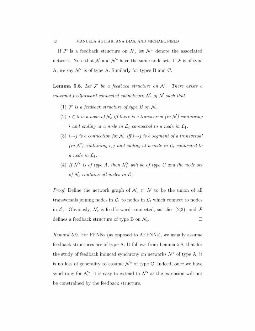
FEEDFORWARD NETWORKS 41
same results hold for J-feedback structures on (A)FFNNs, where 1 6∈ J ,
and we include them for completeness.
Proposition 5.5. If N is a FFNN with a J-feedback structure where
1 6∈ J , with synchrony partition {Pa}a∈s, then each Pa is contained in
a single layer: nodes in different layers are not synchronous.
Proposition 5.6. Let N be an AFFNN with a J-feedback structure
where 1 6∈ J , with synchrony partition {Pa}a∈s. Along any transversal,
there are the following possibilities:
(1) All nodes are synchronous.
(2) An initial segment of the transversal is synchronous, the re-
maining nodes are asynchronous.
(3) All nodes are asynchronous.
The straightforward proofs of the above two propositions use ideas
from [2, Theorem 3.4 & Lemmas 4.7, 4.8] and are omitted.
Here we focus on {1}-feedback structures and henceforth refer to a
{1}-feedback structure as a feedback structure.
Definition 5.7. Let F be a feedback structure on N .
(1) F is of type A if every node in L1 receives at least one connection
from a node in L`.
(2) F is of type B if every node in L` is connected to at least one
node in L1.
(3) F is of type C if it is of type A and B.
42 MANUELA AGUIAR, ANA DIAS, AND MICHAEL FIELD
If F is a feedback structure on N , let N ? denote the associated
network. Note that N and N ? have the same node set. If F is of type
A, we say N ? is of type A. Similarly for types B and C.
Lemma 5.8. Let F be a feedback structure on N . There exists a
maximal feedforward connected subnetwork Nc of N such that
(1) F is a feedback structure of type B on Nc.
(2) i ∈ k is a node of Nc iff there is a transversal (in N ) containing
i and ending at a node in L` connected to a node in L1.
(3) i→j is a connection for Nc iff i→j is a segment of a transversal
(in N ) containing i, j and ending at a node in L` connected to
a node in L1.
(4) If N ? is of type A, then N ?c will be of type C and the node set
of Nc contains all nodes in L1.
Proof. Define the network graph of Nc ⊂ N to be the union of all
transversals joining nodes in L1 to nodes in L` which connect to nodes
in L1. Obviously, Nc is feedforward connected, satisfies (2,3), and F
defines a feedback structure of type B on Nc. �
Remark 5.9. For FFNNs (as opposed to AFFNNs), we usually assume
feedback structures are of type A. It follows from Lemma 5.8, that for
the study of feedback induced synchrony on networks N ? of type A, it
is no loss of generality to assume N ? of type C. Indeed, once we have
synchrony for N ?c , it is easy to extend to N ? as the extension will not
be constrained by the feedback structure.
FEEDFORWARD NETWORKS 43
Lemma 5.10. (Notation and assumptions as above.) Suppose F is a
feedback structure of type C on N . Given i ∈ Lt, j ∈ Lu, there exists
a path γ : i = i0→i1→ . . .→ip = j in the network graph of N ?. The
minimal length p of γ is d` + u − t, where d ∈ {0, 1, 2}, if u ≥ t, and
d ∈ {1, 2} otherwise.
Proof. A straightforward computation using feedforward connectedness
and Remark 5.3. �
5.3. Adaptation on feed forward networks.
Proposition 5.11. (Notation and assumptions as above.) Suppose
that N is an adaptive (A)FFNN with layers L1, . . . ,L` and that the
partition P is a synchrony partition for an initial weight vector. Set
Pt = Lt ∩ P, t ∈ `.
(1) If adaptation is multiplicative, then the synchrony will be pre-
served within layers. That is, the induced partitions Pt are pre-
served for all t ∈ `.
(2) If adaptation is of mixed or additive type and the local in-degrees
ρa,b are constant on layers, then synchrony will be preserved
within layers.
Proof. (1) follows from Theorem 3.3. (2) uses Theorem 3.3 and an easy
induction on layers. �
6. Synchrony for FFNNs with feedback structure.
We continue with the assumptions and notation of the previous sec-
tion and emphasize that N is always assumed feedforward connected.
44 MANUELA AGUIAR, ANA DIAS, AND MICHAEL FIELD
Definition 6.1. Let P = {Pa}a∈s be a synchrony partition for N ?
and suppose d ∈ [1, ` − 1] is a divisor of ` and P 6= {k}—the fully
synchronous partition.
(1) P is layer d-periodic (or layer periodic, period d) if, for all a ∈ s,
and t, u ∈ `.
Pa ∩ Lt 6= ∅ =⇒ Pa ∩ Lu 6= ∅, t ≡ u, mod d.
(d is assumed minimal for this property.)
(2) If P is layer 1-periodic, P is layer complete.
Remark 6.2. If P is layer periodic, then each node in Lt will be syn-
chronized with nodes in other layers. If P is layer complete, then each
node in Lt will be synchronized with nodes in every other layer. In
particular, since a layer complete partition is not the fully synchronous
partition, each layer of N contains at least two nodes.
Examples 6.3. (1) In Figure 10 we show two examples of layer periodic
synchrony partitions for feedforward connected FFNNs with feedback
structure. Connections are labelled with weights and weights are arbi-
trary real numbers with the proviso that weights with the same symbol
must have the same value.
In Figure 10(b), if we move the outputs from the top node in L4
labelled A to the other node labelled A in L4, P is still layer com-
plete. However, the feedback structure is no longer of type B. As in
Lemma 5.8, we can remove the node without outputs and the two nodes
labelled B in the first row, together with associated 6 connections, to
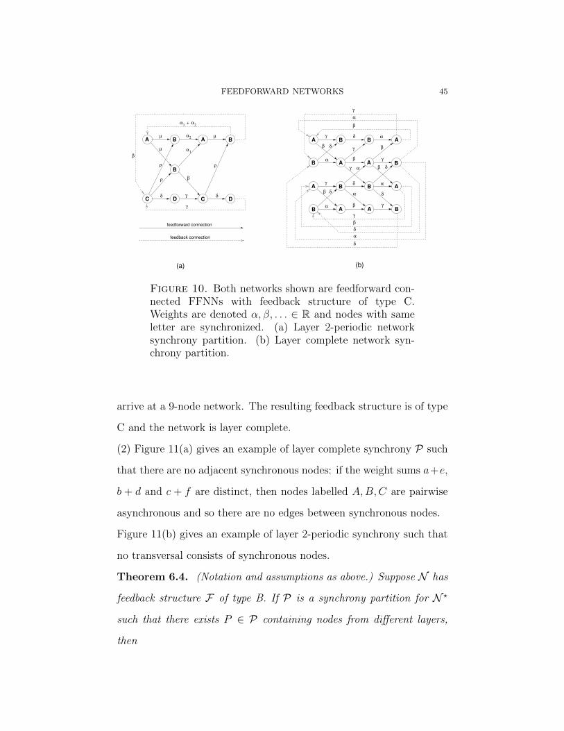
FEEDFORWARD NETWORKS 45
α2
α1
α1 α2+
µ
ρ
ρ
γ
γ
δ δ
ρ
µ
β
µ
β
A AB
B
B
C CD D
feedback connection
feedforward connection
A A
A
A
A
A
A
B
B
B
B
B
B
α
α
γ
γ
γ
αγ β δ
δ
δβ
β
β
δ
β
α
γ
γ
δ
α
β
γ
β
δ
α
δ
β
α
α
δ
γ
B
B
A
(a) (b)
Figure 10. Both networks shown are feedforward con-nected FFNNs with feedback structure of type C.Weights are denoted α, β, . . . ∈ R and nodes with sameletter are synchronized. (a) Layer 2-periodic networksynchrony partition. (b) Layer complete network syn-chrony partition.
arrive at a 9-node network. The resulting feedback structure is of type
C and the network is layer complete.
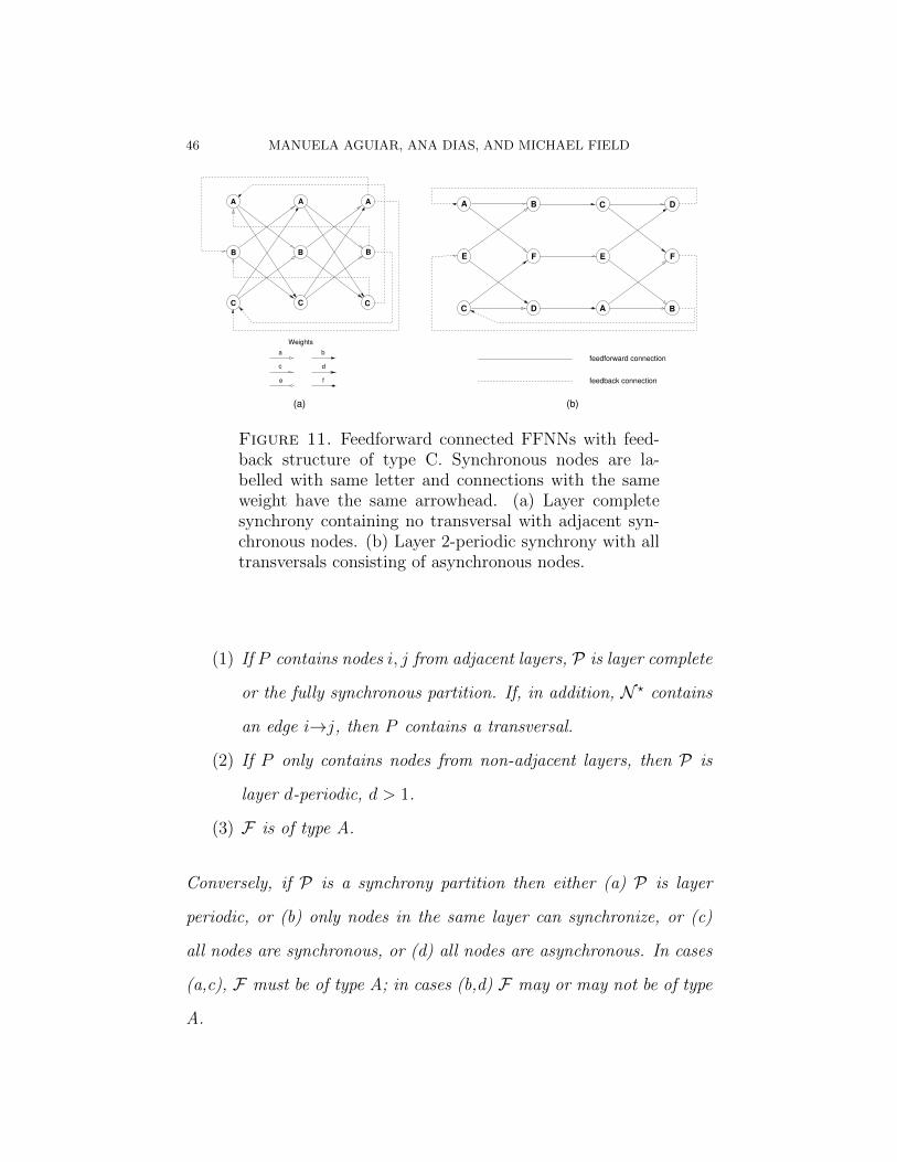
(2) Figure 11(a) gives an example of layer complete synchrony P such
that there are no adjacent synchronous nodes: if the weight sums a+e,
b + d and c + f are distinct, then nodes labelled A,B,C are pairwise
asynchronous and so there are no edges between synchronous nodes.
Figure 11(b) gives an example of layer 2-periodic synchrony such that
no transversal consists of synchronous nodes.
Theorem 6.4. (Notation and assumptions as above.) Suppose N has
feedback structure F of type B. If P is a synchrony partition for N ?
such that there exists P ∈ P containing nodes from different layers,
then
46 MANUELA AGUIAR, ANA DIAS, AND MICHAEL FIELD
A B
B
C
C
D
AD
E F E F
A
B
C
A A
C C
B B
a
c
e
b
d
f
Weights
feedforward connection
feedback connection
(a) (b)
Figure 11. Feedforward connected FFNNs with feed-back structure of type C. Synchronous nodes are la-belled with same letter and connections with the sameweight have the same arrowhead. (a) Layer completesynchrony containing no transversal with adjacent syn-chronous nodes. (b) Layer 2-periodic synchrony with alltransversals consisting of asynchronous nodes.
(1) If P contains nodes i, j from adjacent layers, P is layer complete
or the fully synchronous partition. If, in addition, N ? contains
an edge i→j, then P contains a transversal.
(2) If P only contains nodes from non-adjacent layers, then P is
layer d-periodic, d > 1.
(3) F is of type A.
Conversely, if P is a synchrony partition then either (a) P is layer
periodic, or (b) only nodes in the same layer can synchronize, or (c)
all nodes are synchronous, or (d) all nodes are asynchronous. In cases
(a,c), F must be of type A; in cases (b,d) F may or may not be of type
A.
FEEDFORWARD NETWORKS 47
The proof of Theorem 6.4 depends on a number of subsidiary results
of interest in their own right.
Lemma 6.5. Let N have feedback structure F and P be a synchrony
partition for N ?. If there exists P ∈ P which contains nodes i, j, with
i→j, then there exists a transversal consisting entirely of nodes in P .
We may require that the transversal ends at a node in L` connected to
a node in L1. (The transversal may, or may not, contain i, j.)
Proof. Suppose i ∈ Lt, j ∈ Lt+1. Since i→j and i, j are synchronous,
i must receive an input from a node i′ ∈ Lt−1 ∩ P (if t = 1, i′ ∈ L`).
Proceeding by backwards iteration, we obtain a path
i1→i2→ . . .→i`→ . . .→i→j
in P with i1 ∈ L1 and i` ∈ L`. The required transversal path is
i1→i2→ . . .→i`. �
Remark 6.6. We often use the “backward iteration” technique of the
proof of Lemma 6.5. This method may fail if there are nodes with
self-loops but no other inputs. In particular, no edge in a path should
be a self-loop. This will be important later when we consider AFFNNs
with feedback structures.
Next a useful definition and result.
Definition 6.7. Let N have feedback structure F and P = {Pa}a∈s
be a synchrony partition. Let γ be a path i0→i1→ . . .→iL of length L
in N ? and suppose that iu ∈ Pau , u = 0, . . . , L. A synchrony translate
of γ is a path j0→j1→ . . .→jL such that ju ∈ Pau , u = 0, . . . , L.
48 MANUELA AGUIAR, ANA DIAS, AND MICHAEL FIELD
Lemma 6.8. Let N have feedback structure F and P = {Pa}a∈s be
a synchrony partition. Let γ be a path i0→i1→ . . .→iL in N ? with
ip ∈ Pap, 0 ≤ p ≤ L.
(1) If jL ∈ PaL, there is a synchrony translate j0→j1→ . . .→jL with
jp ∈ Pap, 0 ≤ p ≤ L.
(2) If a0 = aL, there is a synchrony translate j0→j1→ . . .→jL of γ
with jL = i0. Necessarily, j0 ∈ Pa0.
Proof. (1) follows using the standard synchrony based backward itera-
tion argument. Statement (2) is a special case of (1). �
Proposition 6.9. Let N have feedback structure F of type B and P =
{Pa}a∈s be a synchrony partition for N ? with s > 1. Suppose there
exist a ∈ s and nodes i, j ∈ Pa lying in adjacent layers. Then:
(1) If i→j then Pa contains a transversal.
(2) F is of type A.
(3) P is layer complete or the fully synchronous partition.
Proof. (1) By Lemma 6.5, Pa contains a transversal γ.
(2) F is of type B and feedforward connected. Suppose that i ∈ Lp,
j ∈ Lp+1, where i, j ∈ Pa. Take a transversal containing i and let
i′ ∈ Ll ∩ Pb denote the end node of the transversal. Take a synchrony
translate of this transversal through node j and note that there is a
node in j′ ∈ Pb ∩ L1 belonging to this translate. Suppose there is one
node k ∈ L1 not receiving at least one connection from a node of Ll.
Take a transversal from k to i′. The synchrony partition of node k
should be different from any synchrony partition of the other nodes in
FEEDFORWARD NETWORKS 49
that transversal. Indeed, since k has no inputs, the synchrony partition
of k can only occur in the first layer. Take a synchrony translate of
this transversal leading to j′. Then there is a node in L2 in the same
synchrony partition as k, a contradiction. Thus F is of type A.
(3) Since F is of type C, it follows from Lemma 5.10 that there is a
path from i to j. A synchrony translate of this path, starting at node
j, ends at a node in Pa ∩ Lp+2. Iterating this argument, we conclude
that there is at least one node from each layer in Pa. If we take any
node q ∈ Pd, with d 6= a, then we have paths from q to any of the nodes
in Pa in each of the layers. Taking synchrony translates of these paths,
we conclude that Pd contains nodes from every layer and so P is layer
complete or the fully synchronous partition. �
Lemma 6.10. Let N have feedback structure F which is not of type A.
If P = {Pa}a∈s is a synchrony partition, then each Pa ∈ P is contained
in a unique layer Li(a) of L.
Proof. Suppose the contrary. Then, for some a ∈ s, there exist i0, j0 ∈
Pa with i0 ∈ Lt, j0 ∈ Lu, where t < u. Note that if t = 1 there is a
connection from L` to i0—since i0, j0 are synchronous and u > 1. Since
N is feedforward connected, there is a path τ : ip→it−1→ . . .→i0, of
length either t−1 or `+t−1, where ip ∈ L1 has no connections from L`.
By Lemma 6.8(1), there is a synchrony translate jp→jp−1→ . . .→j0 of
τ . But jp /∈ L1 and so has inputs. Contradiction since ip receives no
inputs and so cannot be synchronous with jp. �
Before proving the final result needed for the proof of Theorem 6.4,
we need a definition.
50 MANUELA AGUIAR, ANA DIAS, AND MICHAEL FIELD
Definition 6.11. Let P = {Pa}a∈s be a synchrony partition for N ?
and a ∈ s. If Pa only contains nodes in one layer, set δ(a) = 0, else
define
δ(a) = min{|i− j| | i, j ∈ Pa, where i, j lie in different layers}.
We refer to δ(a) as the synchronization distance for Pa.
Proposition 6.12. Let N have feedback structure F of type B. If P =
{Pa}a∈s is a synchrony partition for N ? and for some a ∈ s, δ(a) =
d > 0, then
(1) F is of type A.
(2) d|`.
(3) P is layer d-periodic and δ : s→N is constant, equal to d.
In particular, if d = 1, P is either layer complete or the fully synchro-
nous partition.
Proof. Property (1) holds by Lemma 6.10. Hence, by Lemma 5.10,
given any two nodes in N ? there is a path connecting them. Suppose
m1, n1 ∈ Pa, where m1 ∈ Lu, n1 ∈ Lu+d, and u ≥ 1 is minimal for
this property. By Lemma 5.10, we may choose a path γ1 of shortest
length joining m1 to n1. If the length of γ1 is L, then L = p` + d,
where 0 ≤ p ≤ 2. By Lemma 6.8(2), we may choose a sequence γj of
synchrony translates of γ1 such that γj will connect mj to nj, where
nj = mj−1, j > 1. If d 6 | `, then for some j > 1 either mj ∈ Lv, for
v < u, or u < v < u+d. In the first case, we contradict the minimality
FEEDFORWARD NETWORKS 51
of u; in the second case we contradict the definition of synchronization
distance. Hence d|`, proving (2).
For (3), suppose that a ∈ s is chosen so that δ(a) is minimal. Suppose
b ∈ s, b 6= a, and choose the minimal v ≥ 1 such that Lv∩Pb 6= ∅. Pick
x ∈ Lv ∩ Pb and path from x to m1 ∈ Lu. Then choose a synchrony
translate of the path to connect some y ∈ Lv+d∩Pb to n1 ∈ Pa. Just as
above, we show that Lv+jd ∩ Pb 6= ∅ for all j ≥ 0. If there were nodes
in other layers, this would contradict the minimality of δ(a). �
Remark 6.13. Let N ? be of type B. If there is a synchrony partition
P for which there exists Pa ∈ P with δ(a) ≥ 2, then it follows from
Proposition 6.12 that ` ≥ 4 and is not prime.
Proof of Theorem 6.4. (1) follows from Propositions 6.12(3),
Proposition 6.9, and Lemma 6.5. (2) follows from Proposition 6.12(3),
(3) follows from Proposition 6.12(1). The converse statements follow
from Lemma 6.10, Proposition 6.12 and Examples 6.3. �
7. Synchrony for AFFNNs with feedback structure
Throughout this section N will be an AFFNN with layer structure
L = {Li}i∈s and F will be a feedback structure on N . Let N ? denote
the associated network. We always assume
(1) N is feedforward connected.
(2) N ? is of type B.
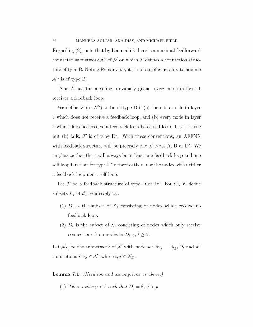
52 MANUELA AGUIAR, ANA DIAS, AND MICHAEL FIELD
Regarding (2), note that by Lemma 5.8 there is a maximal feedforward
connected subnetwork Nc of N on which F defines a connection struc-
ture of type B. Noting Remark 5.9, it is no loss of generality to assume
N ? is of type B.
Type A has the meaning previously given—every node in layer 1
receives a feedback loop.
We define F (or N ?) to be of type D if (a) there is a node in layer
1 which does not receive a feedback loop, and (b) every node in layer
1 which does not receive a feedback loop has a self-loop. If (a) is true
but (b) fails, F is of type D?. With these conventions, an AFFNN
with feedback structure will be precisely one of types A, D or D?. We
emphasize that there will always be at least one feedback loop and one
self loop but that for type D? networks there may be nodes with neither
a feedback loop nor a self-loop.
Let F be a feedback structure of type D or D?. For t ∈ `, define
subsets Dt of Lt recursively by:
(1) D1 is the subset of L1 consisting of nodes which receive no
feedback loop.
(2) Dt is the subset of Lt consisting of nodes which only receive
connections from nodes in Dt−1, t ≥ 2.
Let ND be the subnetwork of N with node set ND = ∪t≥1Dt and all
connections i→j ∈ N , where i, j ∈ ND.
Lemma 7.1. (Notation and assumptions as above.)
(1) There exists p < ` such that Dj = ∅, j > p.
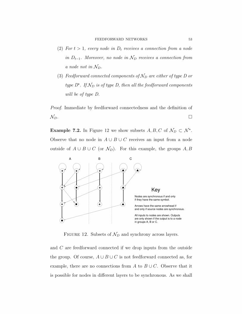
FEEDFORWARD NETWORKS 53
(2) For t > 1, every node in Dt receives a connection from a node
in Dt−1. Moreover, no node in ND receives a connection from
a node not in ND.
(3) Feedforward connected components of ND are either of type D or
type D?. If ND is of type D, then all the feedforward components
will be of type D.
Proof. Immediate by feedforward connectedness and the definition of
ND. �
Example 7.2. In Figure 12 we show subsets A,B,C of ND ⊂ N ?.
Observe that no node in A ∪ B ∪ C receives an input from a node
outside of A ∪ B ∪ C (or ND). For this example, the groups A,B
+
+ +
+
++ +
Nodes are synchronous if and only
if they have the same symbol.
Arrows have the same arrowhead if
and only if source nodes are synchronous.
All inputs to nodes are shown. Outputs
are only shown if the output is to a node
in groups A, B or C.
Key
A B C
Figure 12. Subsets of ND and synchrony across layers.
and C are feedforward connected if we drop inputs from the outside
the group. Of course, A ∪ B ∪ C is not feedforward connected as, for
example, there are no connections from A to B ∪ C. Observe that it
is possible for nodes in different layers to be synchronous. As we shall
54 MANUELA AGUIAR, ANA DIAS, AND MICHAEL FIELD
see, this is essentially the only way a proper subset of nodes in different
layers of a network of type D or D? can be synchronous. In particular,
if no nodes in ND are synchronous, there can be no nodes in different
layers of N ? that are synchronous. We refer to [2] for general results
on synchrony for feedforward connected AFFNN networks.
We define a second subnetwork of N ? which is the maximal subnet-
work of type A. Let F1 ⊂ L1 be the set of all nodes in L1 that receive
a feedback loop. We define the subnetwork NA to consist of all nodes
and edges that belong to transversals from nodes in F1. The feed-
back structure F induces a feedback structure on NA with associated
network N ?A. Denote the node set of N ?
A by NA.
Lemma 7.3. (Notation and assumptions as above.)
(1) NA contains all the nodes in L`.
(2) N ?A is of type A.
(3) The node sets of ND and N ?A (or NA) are disjoint and compli-
mentary.
(4) If P is a synchrony partition for N ?, then PD = P ∩ ND will
be a synchrony partition for ND. Conversely, every synchrony
partition of ND extends to a synchrony partition of N ?.
Proof. For (3), observe that ND receives no inputs from N ?A. All the
remaining statements are routine and we omit proofs. �
Remark 7.4. If N is not of type A, then it is possible that no node in
layer 1 of NA has a self-loop. In this case, possible synchrony for NA
is constrained by Theorem 6.4. Moreover, for this case, we shall show
FEEDFORWARD NETWORKS 55
that nodes in N , which lie in NA, can only be synchronous if they lie
in the same layer. In particular, N cannot be layer periodic or fully
synchronous.
Theorem 7.5. (Assumptions and notation as above.) Let F be a feed-
back structure on the AFFNN N . If P = {Pa}a∈s is a synchrony
partition for N ? then one (at least) of the following possibilities hold.
(1) P is layer complete and F is of type A.
(2) All nodes are synchronous and F is not of type D?.
(3) All nodes are asynchronous and F is of type A, D or D?.
(4) There exists P ∈ P such that P is contained in a layer and is
not a singleton. F can be of type A, D or D?.
(5) If P 6= {k}, F is of type D or D?, and there exist synchronous
nodes i, j in different layers,
(a) i, j ∈ ND and are synchronous in PD = P ∩ND.
(b) If F is not of type D?, the partition PD may be the fully
synchronous partition of ND.
(c) No node in ND can be synchronous with a node in N ?A and
there are no synchronous nodes in different layers of N ?A.
Remarks 7.6. (1) One only of (1–3) of Theorem 7.5 can occur and then
(4,5) do not occur. On the other hand, (4) and (5) may both occur
multiple times for the same synchrony partition. Note that if N ? is of
type A, then ND = ∅.
(2) If no node in layer 1 of NA has a self loop, it is easy to find examples
where every layer of N ? contains at least two synchronous nodes.
(3) Synchrony for feedforward connected AFFNNs is classified in [2,
56 MANUELA AGUIAR, ANA DIAS, AND MICHAEL FIELD
§4] and these results can be used to enumerate synchrony partitions
for a specific network ND.
The following results are corollaries of Theorem 7.5.
Corollary 7.7. Let F be a feedback structure on the AFFNN N such
that at least one node in the first layer does not receive a feedback
loop. Given a synchrony partition for N ?, we have precisely one of the
following possibilities:
(a) All nodes are synchronous.
(b) Only nodes in the same layer can be synchronous.
(c) All nodes are asynchronous.
(d) There is a transversal γ with proper initial segment γi ⊂ ND
consisting of synchronous nodes with the remaining nodes of γ
being asynchronous. Any synchronous nodes lying in different
layers of N lie in ND.
Corollary 7.8. Let F be a feedback structure on the AFFNN N of
type A. Consider a synchrony partition for N ?. We have precisely one
of the following possibilities:
(a) The synchrony partition is layer complete. In particular, all
nodes can be synchronous.
(b) Only nodes in the same layer can synchronize.
(c) All nodes are asynchronous.
Examples 7.9. In Figure 13 we show two examples of AFFNNs with
feedback. Network (a) is of type D, network (b) is of type A.
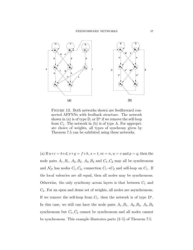
FEEDFORWARD NETWORKS 57
A1
A2
A3
B3
B1
B2
u
c
w v
x
dw*
x* u*
v*
a b
A1
A2
A3
B3
C2
C1
B1
B2
a d
cb
ge h
u v
t
p
fs
qm n
(a) (b)
Figure 13. Both networks shown are feedforward con-nected AFFNNs with feedback structure. The networkshown in (a) is of type D, or D? if we remove the self-loopfrom C1. The network in (b) is of type A. For appropri-ate choice of weights, all types of synchrony given byTheorem 7.5 can be exhibited using these networks.
(a) If a+c = b+d, e+g = f+h, s = t, m = n, u = v and p = q, then the
node pairs A1, B1, A2, B2, A3, B3 and C1, C2 may all be synchronous
and ND has nodes C1, C2, connection C1→C2 and self-loop on C1. If
the local valencies are all equal, then all nodes may be synchronous.
Otherwise, the only synchrony across layers is that between C1 and
C2. For an open and dense set of weights, all nodes are asynchronous.
If we remove the self-loop from C1, then the network is of type D?.
In this case, we still can have the node pairs A1, B1, A2, B2, A3, B3
synchronous but C1, C2 cannot be synchronous and all nodes cannot
be synchronous. This example illustrates parts (3–5) of Theorem 7.5.
58 MANUELA AGUIAR, ANA DIAS, AND MICHAEL FIELD
(b) If a = w = w?, b = v = v?, c = x = x?, d = u = u?, then
{{A1, B2, A3}, {B1, A2, B3}} is a layer complete synchrony partition.
If the valencies are constant on layers but differ between layers, then
{{Ai, Bi} | i ∈ 3} will be a synchrony partition and nodes can be only
synchronous if they are in the same layer. If x? = v?, u? = w?, u 6= w,
a 6= d, then nodes in layer 3 can be synchronous with all other nodes
asynchronous. For an open and dense set of weights, all nodes will
be asynchronous. This example illustrates (1–4) of Theorem 7.5 for
networks of type A.
The proof of Theorem 7.5 depends on some preliminary results.
The definition of synchrony translate continues to hold for AFFNNs
with a feedback structure and it is easy to see that Lemma 5.10 remains
valid for AFFNNs with feedback structure of type A. Lemma 6.8 holds
for AFFNNs with feedback structure of type A if, for example, adjacent
nodes on the path are not synchronous.
Proposition 7.10. Let F be a feedback structure of type A on the
AFFNN N . Suppose P is a synchrony partition for N ?. If there ex-
ist synchronous nodes lying in different layers then P is either layer
complete or the fully synchronous partition. In either case there is a
transversal consisting of synchronous nodes.
Proof. Suppose first that there is no pair of adjacent synchronous nodes
but there exists at least one pair of synchronous nodes lying in different
layers. Lemma 6.8(1) applies and we may follow the proof of Proposi-
tion 6.12 to obtain an integer d ∈ [1, ` − 1], d|`, such that P is layer
FEEDFORWARD NETWORKS 59
d-periodic. Let i ∈ L1 have a self-loop (at least one such node exists
since N is an AFFNN). It follows by d-periodicity that there is a node
j ∈ Ld+1 which is synchronous to i. Since i ∈ L1 has a self-loop, there
must be a node i′ ∈ Ld which is synchronous with j and adjacent to j.
Contradiction.
It follows that if there exists a pair of synchronous nodes lying in
different layers, then there must exist a pair i, j of adjacent synchronous
nodes lying in adjacent layers. Suppose that i→j and i ∈ Lt, j ∈ Lt+1,
where t ∈ [1, `] (t + 1 is computed mod `). By backward iteration, we
obtain a path of adjacent synchronous nodes i1→ . . .→it = i→it+1 = j
and so a synchronous transversal if t ∈ {`− 1, `}. Suppose we cannot
find adjacent i, j with t ∈ {`−1, `}. Let T ∈ [2, `−2] be the maximum
value of t for which there exists an adjacent pair of i, j of synchronous
nodes with i ∈ Lt, j ∈ Lt+1. By Lemma 5.10, we may choose a
path τ : j→ . . .→i of length L = ` − 1, mod `. By our maximality
assumption, τ will contain no pairs a, b of adjacent synchronous nodes
with a ∈ Ls, b ∈ Ls+1, s ∈ [T + 1, `]. It follows that Lemma 6.8
applies to give a translate j′1→ . . .→j′L = j of τ . Hence there exists
j′ = j′1 ∈ LT+2 which is synchronous to j. Therefore, by synchrony,
there exists i′ ∈ LT+1 which is synchronous to j′ and adjacent to j′,
contradicting the maximality of T .
Our arguments show that if there exist synchronous nodes lying in
different layers there is a transversal consisting of synchronous nodes.
Now apply the argument of Proposition 6.9 to deduce that P is either
layer complete or the fully synchronous partition. �
60 MANUELA AGUIAR, ANA DIAS, AND MICHAEL FIELD
Lemma 7.11. Let F be a feedback structure on the AFFNN N of type
D or D? and P be a synchrony partition for N ?.
(1) If N ? is of type D and there is a node in N ?A synchronous with
a node in ND, then all nodes are synchronous: P = {k}.
(2) If N ? is of type D?, it is not possible for a node in N ?A to be
synchronous with a node in ND.
Proof. Suppose i ∈ N ?A and j ∈ ND are synchronous. Choose a closed
path γ : i = i0→i1→ . . .→iL = i which necessarily is contained in
N ?A since the nodes in layer 1 of ND can only have a self-loop but
no feedback loop. Since j is synchronous with i, we can lift the final
segment of γ to a path τ = jp→ . . .→j0 = s where jr ∈ ND and is
synchronous with iL−r, 0 ≤ r ≤ p, and jp ∈ L1. Either jp has no self-
loop—contradicting the synchrony of jp and iL−p or jp has a self loop.
In the latter case all the nodes i0, . . . , iL−p all receive inputs but only
from nodes synchronous to i. Hence γ consists of nodes synchronous
to i. Since γ contains a transversal of synchronous nodes, it follows
easily by feedforward connectedness that P = {k}. In particular, N ?
is of type D since a network of type D? has a node with no input. �
Lemma 7.12. Let F be a feedback structure on the AFFNN N of type
D or D? and P be a synchrony partition for N ?. If there is a pair of
synchronous nodes in N ?A lying in different layers, then P = {k} and
F is of type D.
Proof. From Proposition 7.10 we have that the synchrony partition for
N ?A is either layer complete or the fully synchronous partition. From
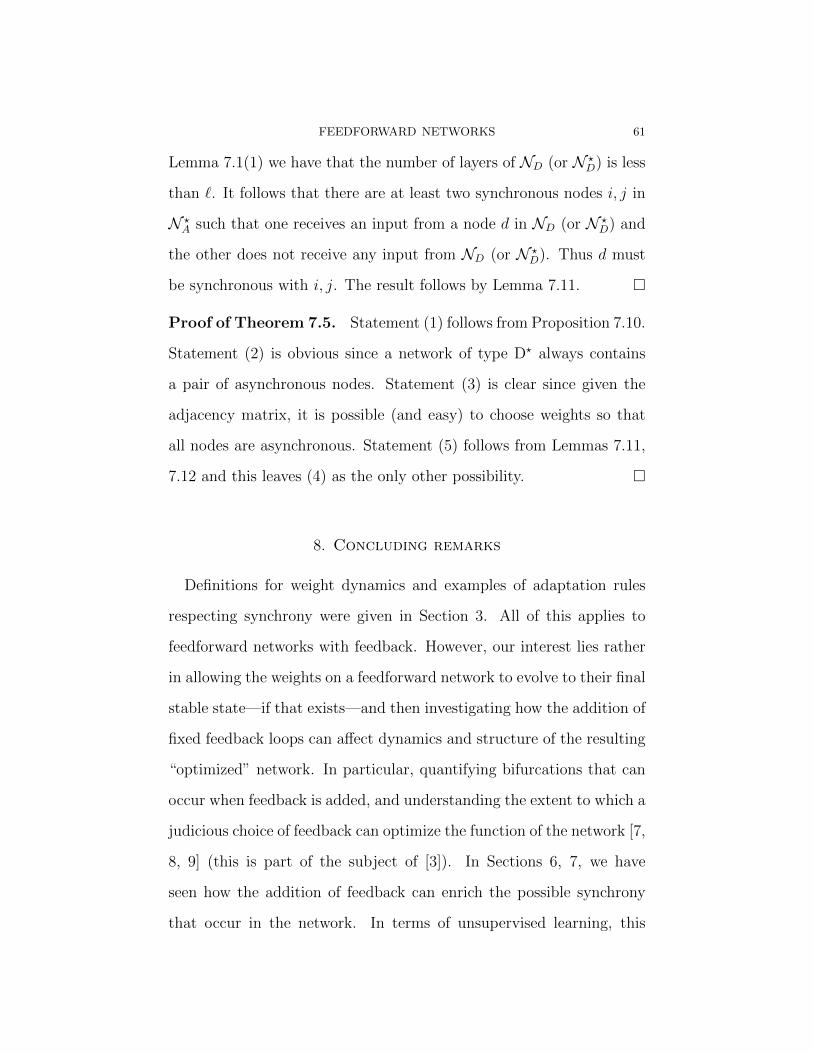
FEEDFORWARD NETWORKS 61
Lemma 7.1(1) we have that the number of layers of ND (or N ?D) is less
than `. It follows that there are at least two synchronous nodes i, j in
N ?A such that one receives an input from a node d in ND (or N ?
D) and
the other does not receive any input from ND (or N ?D). Thus d must
be synchronous with i, j. The result follows by Lemma 7.11. �
Proof of Theorem 7.5. Statement (1) follows from Proposition 7.10.
Statement (2) is obvious since a network of type D? always contains
a pair of asynchronous nodes. Statement (3) is clear since given the
adjacency matrix, it is possible (and easy) to choose weights so that
all nodes are asynchronous. Statement (5) follows from Lemmas 7.11,
7.12 and this leaves (4) as the only other possibility. �
8. Concluding remarks
Definitions for weight dynamics and examples of adaptation rules
respecting synchrony were given in Section 3. All of this applies to
feedforward networks with feedback. However, our interest lies rather
in allowing the weights on a feedforward network to evolve to their final
stable state—if that exists—and then investigating how the addition of
fixed feedback loops can affect dynamics and structure of the resulting
“optimized” network. In particular, quantifying bifurcations that can
occur when feedback is added, and understanding the extent to which a
judicious choice of feedback can optimize the function of the network [7,
8, 9] (this is part of the subject of [3]). In Sections 6, 7, we have
seen how the addition of feedback can enrich the possible synchrony
that occur in the network. In terms of unsupervised learning, this
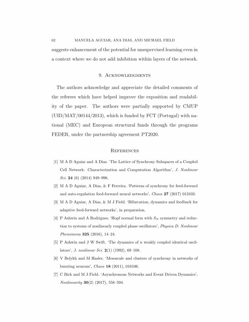
62 MANUELA AGUIAR, ANA DIAS, AND MICHAEL FIELD
suggests enhancement of the potential for unsupervised learning even in
a context where we do not add inhibition within layers of the network.
9. Acknowledgments
The authors acknowledge and appreciate the detailed comments of
the referees which have helped improve the exposition and readabil-
ity of the paper. The authors were partially supported by CMUP
(UID/MAT/00144/2013), which is funded by FCT (Portugal) with na-
tional (MEC) and European structural funds through the programs
FEDER, under the partnership agreement PT2020.
References
[1] M A D Aguiar and A Dias. ‘The Lattice of Synchrony Subspaces of a Coupled
Cell Network: Characterization and Computation Algorithm’, J. Nonlinear
Sci. 24 (6) (2014) 949–996.
[2] M A D Aguiar, A Dias, & F Ferreira. ‘Patterns of synchrony for feed-forward
and auto-regulation feed-forward neural networks’, Chaos 27 (2017) 013103.
[3] M A D Aguiar, A Dias, & M J Field. ‘Bifurcation, dynamics and feedback for
adaptive feed-forward networks’, in preparation.
[4] P Ashwin and A Rodrigues. ‘Hopf normal form with SN symmetry and reduc-
tion to systems of nonlinearly coupled phase oscillators’, Physica D: Nonlinear
Phenomena 325 (2016), 14–24.
[5] P Ashwin and J W Swift. ‘The dynamics of n weakly coupled identical oscil-
lators’, J. nonlinear Sci. 2(1) (1992), 69–108.
[6] V Belykh and M Hasler. ‘Mesoscale and clusters of synchrony in networks of
bursting neurons’, Chaos 18 (2011), 016106.
[7] C Bick and M J Field. ‘Asynchronous Networks and Event Driven Dynamics’,
Nonlinearity 30(2) (2017), 558–594.
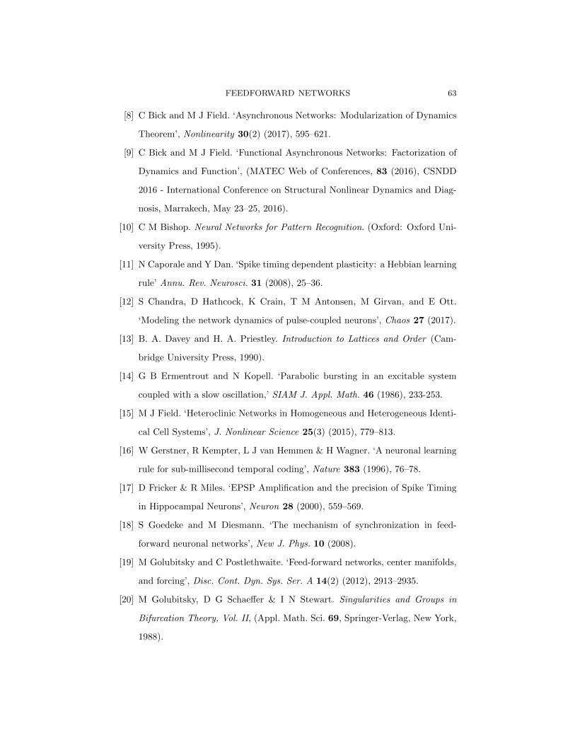
FEEDFORWARD NETWORKS 63
[8] C Bick and M J Field. ‘Asynchronous Networks: Modularization of Dynamics
Theorem’, Nonlinearity 30(2) (2017), 595–621.
[9] C Bick and M J Field. ‘Functional Asynchronous Networks: Factorization of
Dynamics and Function’, (MATEC Web of Conferences, 83 (2016), CSNDD
2016 - International Conference on Structural Nonlinear Dynamics and Diag-
nosis, Marrakech, May 23–25, 2016).
[10] C M Bishop. Neural Networks for Pattern Recognition. (Oxford: Oxford Uni-
versity Press, 1995).
[11] N Caporale and Y Dan. ‘Spike timing dependent plasticity: a Hebbian learning
rule’ Annu. Rev. Neurosci. 31 (2008), 25–36.
[12] S Chandra, D Hathcock, K Crain, T M Antonsen, M Girvan, and E Ott.
‘Modeling the network dynamics of pulse-coupled neurons’, Chaos 27 (2017).
[13] B. A. Davey and H. A. Priestley. Introduction to Lattices and Order (Cam-
bridge University Press, 1990).
[14] G B Ermentrout and N Kopell. ‘Parabolic bursting in an excitable system
coupled with a slow oscillation,’ SIAM J. Appl. Math. 46 (1986), 233-253.
[15] M J Field. ‘Heteroclinic Networks in Homogeneous and Heterogeneous Identi-
cal Cell Systems’, J. Nonlinear Science 25(3) (2015), 779–813.
[16] W Gerstner, R Kempter, L J van Hemmen & H Wagner. ‘A neuronal learning
rule for sub-millisecond temporal coding’, Nature 383 (1996), 76–78.
[17] D Fricker & R Miles. ‘EPSP Amplification and the precision of Spike Timing
in Hippocampal Neurons’, Neuron 28 (2000), 559–569.
[18] S Goedeke and M Diesmann. ‘The mechanism of synchronization in feed-
forward neuronal networks’, New J. Phys. 10 (2008).
[19] M Golubitsky and C Postlethwaite. ‘Feed-forward networks, center manifolds,
and forcing’, Disc. Cont. Dyn. Sys. Ser. A 14(2) (2012), 2913–2935.
[20] M Golubitsky, D G Schaeffer & I N Stewart. Singularities and Groups in
Bifurcation Theory, Vol. II, (Appl. Math. Sci. 69, Springer-Verlag, New York,
1988).
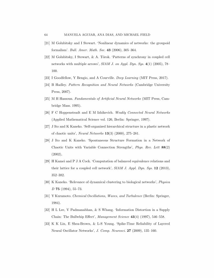
64 MANUELA AGUIAR, ANA DIAS, AND MICHAEL FIELD
[21] M Golubitsky and I Stewart. ‘Nonlinear dynamics of networks: the groupoid
formalism’. Bull. Amer. Math. Soc. 43 (2006), 305–364.
[22] M Golubitsky, I Stewart, & A. Torok. ‘Patterns of synchrony in coupled cell
networks with multiple arrows’, SIAM J. on Appl. Dyn. Sys. 4(1) (2005), 78–
100.
[23] I Goodfellow, Y Bengio, and A Courville. Deep Learning (MIT Press, 2017).
[24] B Hadley. Pattern Recognition and Neural Networks (Cambridge University
Press, 2007).
[25] M H Hassoun. Fundamentals of Artificial Neural Networks (MIT Press, Cam-
bridge Mass. 1995).
[26] F C Hoppensteadt and E M Izhikevich. Weakly Connected Neural Networks
(Applied Mathematical Science vol. 126, Berlin: Springer, 1997).
[27] J Ito and K Kaneko. ‘Self-organized hierarchical structure in a plastic network
of chaotic units’, Neural Networks 13(3) (2000), 275–281.
[28] J Ito and K Kaneko. ‘Spontaneous Structure Formation in a Network of
Chaotic Units with Variable Connection Strengths’, Phys. Rev. Lett 88(2)
(2002),
[29] H Kamei and P J A Cock. ‘Computation of balanced equivalence relations and
their lattice for a coupled cell network’, SIAM J. Appl. Dyn. Sys. 12 (2013),
352–382.
[30] K Kaneko. ‘Relevance of dynamical clustering to biological networks’, Physica
D 75 (1994), 55–73.
[31] Y Kuramoto. Chemical Oscillations, Waves, and Turbulence (Berlin: Springer,
1984).
[32] H L Lee, V Padmanabhan, & S Whang. ‘Information Distortion in a Supply
Chain: The Bullwhip Effect’, Management Science 43(4) (1997), 546–558.
[33] K K Lin, E Shea-Brown, & L-S Young. ‘Spike-Time Reliability of Layered
Neural Oscillator Networks’, J. Comp. Neurosci. 27 (2009), 135–160.
FEEDFORWARD NETWORKS 65
[34] T Masquelier, R Guyonneau, & S J Thorpe. ‘Spike Timing Dependent Plastic-
ity Finds the Start of Repeating Patterns in Continuous Spike Trains’, PLoS
ONE 3(1) (2008), e1377.
[35] T Masquelier, R Guyonneau, & S J Thorpe. ‘Competitive STDP-Based Spike
Pattern Learning’, Neural Computation 21(5) (2009), 1259–1276
[36] T Masquelier, E Hugues, G Deco & S J Thorpe. ‘Oscillations, Phase-of-
Firing-Coding, and Spike Timing-Dependent Plasticity: An Efficieint Learning
Scheme’, J. of Neuroscience 29(43) (2009), 13484–13493.
[37] M Minsky and S Papert. Perceptrons: An introduction to Computational Ge-
ometry (MIT press, 1969).
[38] A Morrison, M Diesmann, & W Gerstner. ‘Phenomenological models of synap-
tic plasticity based on spike timing’, Biol. Cybern. (2008), 459-478.
[39] M J Panaggio and D M Abrams. ‘Chimera states: coexistence of coherence
and incoherence in networks of coupled oscillators’, Nonlinearity 28(3) (2015),
R67.
[40] Pedantic of Purley. ‘Uncircling the Circle: Part I’. (On line article
https://www.londonreconnections.com/2013/uncircling-circle-part-1/, in Lon-
don Reconnections, October 3, 2013.)
[41] B Rink and J Sanders. ‘Amplified Hopf bifurcations in feed-forward networks’,
SIAM J. Appl. Dyn. Sys. 12(2) (2013), 1135–1157.
[42] F Rosenblatt. ‘The Perceptron: A Probabilistic Model For Information Storage
And Organization In The Brain’. Psych. Rev. 65(6) (1958), 386–408.
[43] P Sailamul, J Jang, & S-B Paik. ‘Synaptic convergence regulates
synchronization-dependent spike transfer in feedforward neural networks’, J.
Comput. Neurosci. 43 (2017), 189–202.
[44] J Schmidhuber. ‘Deep Learning in Neural Networks: An Overview’. Neural
Networks 61 (2015), 85-117.
[45] I Stewart. ‘The lattice of balanced equivalence relations of a coupled cell net-
work’, Math. Proc. Cambridge Philos. Soc. 143 (1) (2007), 165–183.

66 MANUELA AGUIAR, ANA DIAS, AND MICHAEL FIELD
[46] I Stewart, M Golubitsky, & M. Pivato. ‘Symmetry groupoids and patterns of
synchrony in coupled cell networks’, SIAM J. on Appl. Dyn. Sys. 2(4) (2003),
609–646.
[47] F Takens. Detecting strange attractors in turbulence (Lecture Notes in Math-
ematics 898, Berlin:Springer-Verlag, 1981).
Manuela Aguiar, Faculdade de Economia, Centro de Matematica,
Universidade do Porto, Rua Dr Roberto Frias, 4200-464 Porto, Por-
tugal.
E-mail address: [email protected]
Ana Dias, Departamento de Matematica, Centro de Matematica,
Universidade do Porto, Rua do Campo Alegre, 687, 4169-007 Porto,
Portugal
E-mail address: [email protected]
Michael Field, Department of Mathematics, Imperial College, South
Kensington Campus, London SW7 2AZ, UK
Current address: Department of Mathematics, Rice University MS-136, 6100
Main St., Houston, TX 77005, USA
E-mail address: [email protected]