Feedback Control of Brownian Motion for Single-Particle ...

Feedback Control of Brownian Motion for

Single-Particle Fluorescence Spectroscopy

Thesis by

Andrew J. Berglund

In Partial Fulfillment of the Requirements

for the Degree of

Doctor of Philosophy

California Institute of Technology

Pasadena, CA

2007

(Defended September 27, 2006)

ii

c© 2007

Andrew J. Berglund

All Rights Reserved

iii

Acknowledgements

My years in graduate school have been exciting, challenging, and above all, rewarding,

and for all of these things I have my advisor to thank. Hideo has always given me

the freedom to follow my instincts as a scientist, even from my very first days at Cal-

tech when such trust could not have stemmed from anything more than good-natured

optimism. His willingness to treat students as colleagues and not subordinates is a

unique and extraordinary trait, and the experience of working with him through the

formative years of my career as a scientist and his as an advisor has been incompa-

rable.

My time at Caltech has been influenced almost as much by Hideo’s guidance as

an advisor as by the outstanding group of students and postdocs he has assembled.

We have always had a close-knit group, and every member has brought something

unique into the fold. Thank you to Ramon van Handel, Asa Hopkins, Nathan Hodas,

Tony Miller, Nicole Czakon, Joe Kerckhoff, and to Luc Bouten, Andre Conjusteau,

Andrew Doherty, J.M. Geremia, Chungsok Lee, Jennifer Sokol, Jon Williams, and

Naoki Yamamoto. Much credit should go to Sheri Stoll, our peerless administrator,

for keeping the group running seamlessly. Kevin McHale, whose addition to the

experiment made an immediate positive impact, has been a top-notch lab partner

and friend. Jason McKeever and Chin-Wen “James” Chou, group members in spirit,

if not officially, have been great colleagues and great friends. And to the grad students

I have worked with since day one: Mike Armen, John Au, Ben Lev, John Stockton,

and Tim McGarvey, I can only say that wherever I go, I will be lucky to find just one

person as talented, likeable, and, well, “foolish,” as you guys.

My scientific perspective has been greatly enhanced by interactions with a number

iv

of excellent researchers outside our group, including Erik Winfree, Niles Pierce, Bernie

Yurke, Rob Phillips, Igor Mezic, Atac Imamoglu, Salman Habib, Miles Blencowe, Sean

Andersson, Shimon Weiss, Adam Cohen, and W. E. Moerner. And life has been made

much more enjoyable by a number of good friends, in particular, Nathan Lundblad

and Ian Swanson at Caltech, and Austin Schenk, James May, and Chris Johnson, my

best friends and medical cohorts, scattered across the country but never more than a

phone call away.

Finally, thank you to my family. Thank you to my sisters, Kay and Liz and to

your families; and thank you especially to my parents, John and Mary Kate, who I

can say in full literality have loved, supported, and encouraged me for longer than I

can remember. And to my wife Kim, my newest family member, thank you for not

just putting up with my long hours and frequent distractions, but for marrying me

along the way! I could not have asked for a more perfect person with whom to share

my work, my thoughts, and my life.

v

Abstract

The stochastic Brownian motion of individual particles in solution constrains the

utility of single-particle fluorescence microscopy both by limiting the dwell time of

particles in the observation volume and by convolving their internal degrees of free-

dom with their random spatial trajectories. This thesis describes the use of active

feedback control to eliminate these undesirable effects. We designed and implemented

a feedback tracking system capable of locking the position of a fluorescent particle to

the optic axis of our microscope, i.e., capable of tracking the two-dimensional, planar

Brownian motion of a free particle in solution. A full theoretical description of the

experiment is given in the language of linear stochastic control theory. The model

describes both the statistics of the tracking system and provides a generalization of

the theory of open-loop Fluorescence Correlation Spectroscopy (FCS) that accounts

for fluctuations in fluorescence arising from competition between diffusion and damp-

ing. We find excellent agreement between theory and experiment. Using fluorescent

polymer microspheres as test particles, we find that the observation time for these

particles can be increased by 2–3 orders of magnitude over the open-loop scenario.

The system achieves nearly optimal performance for moderately fast-moving particles

at very low fluorescent count rates, comparable to those of a single fluorescent protein

molecule. The system can classify particles in a binary mixture based on a real-time

estimate of their diffusion coefficients (differing by a factor of ∼4), achieving 90%

success using fewer than 600 photons detected over 120 ms. Future directions for

both the experimental and theoretical techniques are briefly discussed.

vii

Contents

Acknowledgements iii

Abstract v

Contents vii

List of Figures xi

List of Tables xv

Preface xvii

1 Introduction and Motivation 1

1.1 Why collect fluorescence from single molecules? . . . . . . . . . . . . 1

1.2 Fluctuations due to particle diffusion . . . . . . . . . . . . . . . . . . 2

1.3 Fluctuations due to photon counting statistics . . . . . . . . . . . . . 6

1.4 Context and relation to other work . . . . . . . . . . . . . . . . . . . 10

1.5 Publications from graduate work . . . . . . . . . . . . . . . . . . . . 13

I Theory 15

2 Feasibility Study: LQG Controller Design 17

2.1 State-space dynamics and position estimation . . . . . . . . . . . . . 18

2.2 Optimal LQG control . . . . . . . . . . . . . . . . . . . . . . . . . . . 23

2.3 Performance analysis . . . . . . . . . . . . . . . . . . . . . . . . . . . 27

viii

3 Sensing the Position of a Fluorescent Particle 33

3.1 Rate-modulated Poisson statistics . . . . . . . . . . . . . . . . . . . . 35

3.2 Power spectrum of a rate-modulated Poisson process . . . . . . . . . 37

3.3 Application to position sensing . . . . . . . . . . . . . . . . . . . . . 41

3.4 Autocorrelation functions: More statistics! . . . . . . . . . . . . . . . 44

4 Tracking Limits: Photon Counting Noise 51

4.1 Static position estimation . . . . . . . . . . . . . . . . . . . . . . . . 52

4.2 Dynamic position estimation . . . . . . . . . . . . . . . . . . . . . . . 57

4.3 Optimal position estimation . . . . . . . . . . . . . . . . . . . . . . . 62

4.4 Numerical simulations . . . . . . . . . . . . . . . . . . . . . . . . . . 63

4.5 Commentary . . . . . . . . . . . . . . . . . . . . . . . . . . . . . . . 67

5 Full Linear Theory of Closed-Loop Particle Tracking 71

5.1 Linear control system model . . . . . . . . . . . . . . . . . . . . . . . 71

5.1.1 Specification of transfer functions . . . . . . . . . . . . . . . . 73

5.1.2 State-space realizations and the Fokker-Planck equation . . . 75

5.1.3 Marginally stable systems . . . . . . . . . . . . . . . . . . . . 78

5.1.4 Statistics of X(t) and E(t) for low-order systems . . . . . . . 80

5.2 Closed-loop Fluorescence Correlation Spectroscopy . . . . . . . . . . 83

5.2.1 Calculation of the fluorescence autocorrelation function . . . . 84

5.2.2 Recovery of open-loop results in the weak-tracking limit . . . 87

5.2.3 Behavior of g(τ) for τ ≈ 0 . . . . . . . . . . . . . . . . . . . . 88

5.2.4 Relation to other literature results . . . . . . . . . . . . . . . 90

II Experiment 91

6 Experimental Apparatus 93

6.1 Laboratory components . . . . . . . . . . . . . . . . . . . . . . . . . 93

6.1.1 Optics . . . . . . . . . . . . . . . . . . . . . . . . . . . . . . . 93

6.1.2 Sample volume . . . . . . . . . . . . . . . . . . . . . . . . . . 98

ix

6.1.3 Electronics . . . . . . . . . . . . . . . . . . . . . . . . . . . . . 100

6.1.4 Data acquisition and computer software . . . . . . . . . . . . 104

6.2 Calibration and diagnostics . . . . . . . . . . . . . . . . . . . . . . . 107

6.2.1 Open-loop measurements . . . . . . . . . . . . . . . . . . . . . 107

6.2.2 Measuring the error signal . . . . . . . . . . . . . . . . . . . . 112

7 Closed-Loop Particle Tracking 115

7.1 Closing the loop . . . . . . . . . . . . . . . . . . . . . . . . . . . . . . 115

7.2 Early experimental success . . . . . . . . . . . . . . . . . . . . . . . . 116

7.2.1 Tracking data . . . . . . . . . . . . . . . . . . . . . . . . . . . 117

7.2.2 Estimation of D . . . . . . . . . . . . . . . . . . . . . . . . . . 118

7.2.3 Fluorescence fluctuations and Tracking-FCS . . . . . . . . . . 121

7.3 Tracking improvement . . . . . . . . . . . . . . . . . . . . . . . . . . 122

7.4 Comparison with the theory . . . . . . . . . . . . . . . . . . . . . . . 128

8 Detailed Studies of a Binary Mixture 133

8.1 Raw data . . . . . . . . . . . . . . . . . . . . . . . . . . . . . . . . . 133

8.2 Near-optimal tracking . . . . . . . . . . . . . . . . . . . . . . . . . . 147

8.3 Classification by diffusion coefficient estimation . . . . . . . . . . . . 150

8.3.1 Statistics of D∆t . . . . . . . . . . . . . . . . . . . . . . . . . 151

8.3.2 Hypothesis testing . . . . . . . . . . . . . . . . . . . . . . . . 156

8.3.3 Results . . . . . . . . . . . . . . . . . . . . . . . . . . . . . . . 158

8.4 Summary and commentary . . . . . . . . . . . . . . . . . . . . . . . . 160

A Closed-Loop Correlation Spectroscopy with Internal State Transi-

tions 163

A.1 Review of the scalar case and statement of the general problem . . . 164

A.2 The commuting case [F1,F2] = 0 . . . . . . . . . . . . . . . . . . . . . 167

A.3 Adiabatic elimination of fast dynamics . . . . . . . . . . . . . . . . . 170

A.4 Generalization of van Kampen’s method to the noncommuting case . 173

References 179

xi

List of Figures

1.1 Schematic diagram of a free-diffusion SMD apparatus . . . . . . . . . . 3

1.2 Single particle Brownian trajectory through a Gaussian laser . . . . . . 4

1.3 Fluorescence intensity fluctuations of a particle in a Gaussian laser . . 5

1.4 Signal-to-noise ratio SNR of the autocorrelation of a Poisson process

given . . . . . . . . . . . . . . . . . . . . . . . . . . . . . . . . . . . . . 9

2.1 Bode plot of the transfer function T (s) . . . . . . . . . . . . . . . . . . 19

2.2 Schematic diagram of the coordinates used for two-dimensional tracking 22

2.3 Bode diagrams of the transfer function Hλ(s) . . . . . . . . . . . . . . 27

2.4 Simulated tracking performance in two dimensions . . . . . . . . . . . 28

2.5 Radial tracking error eτ over a range of diffusion coefficients . . . . . . 29

3.1 Example of a rate-modulated Poisson process . . . . . . . . . . . . . . 34

3.2 Particle tracking coordinates in the reference frame of the laser . . . . 42

3.3 Mappings between the (ρ, θ) and (x, y) planes . . . . . . . . . . . . . . 43

3.4 gx(τ) for a single immobilized particle in a rotating laser . . . . . . . . 47

4.1 Expectation value of the position estimator E[xt] . . . . . . . . . . . . 55

4.2 Numerical simulation of xt . . . . . . . . . . . . . . . . . . . . . . . . . 57

4.3 Mean-square tracking error E[e2t ] as a function of bandwidth B . . . . 58

4.4 Two-dimensional tracking simulation in the linear regime . . . . . . . . 64

4.5 Two-dimensional tracking simulation in the nonlinear regime . . . . . . 65

4.6 Numerical simulation showing tracked and untracked regimes . . . . . 68

4.7 Tracking phase diagram in the D-B plane . . . . . . . . . . . . . . . . 69

xii

5.1 Block diagram of the particle tracking control system. . . . . . . . . . 72

6.1 Schematic diagram of the optics for single-particle tracking . . . . . . . 94

6.2 Schematic diagram of the sample volume for single-particle tracking . . 99

6.3 Schematic diagram of the electronics for single-particle tracking . . . . 101

6.4 Controller transfer function implemented on the digital microcontroller 103

6.5 Open-loop transit of a 60 nm microsphere through the excitation volume 107

6.6 Open-loop transit of a 60 nm microsphere through a rotating excitation

laser . . . . . . . . . . . . . . . . . . . . . . . . . . . . . . . . . . . . . 108

6.7 Open-loop FCS curve . . . . . . . . . . . . . . . . . . . . . . . . . . . 109

6.8 Open-loop FCS curve with the rotating laser . . . . . . . . . . . . . . . 110

6.9 Measured laser intensity profile for the stationary beam . . . . . . . . . 111

6.10 Measured laser intensity profile for the rotating beam . . . . . . . . . . 111

6.11 Measured error signal for closed-loop tracking . . . . . . . . . . . . . . 112

7.1 Bode plot of the closed-loop transfer function of the tracking system . 116

7.2 Qualitative shape of a closed-loop transfer function . . . . . . . . . . . 117

7.3 Fluorescence intensity and sample stage position from an early tracking

run . . . . . . . . . . . . . . . . . . . . . . . . . . . . . . . . . . . . . . 118

7.4 Diffusion coefficient estimate for the data in Fig. 7.3 . . . . . . . . . . 119

7.5 Fluorescence correlation function for the data in Fig. 7.3 . . . . . . . . 121

7.6 Improved tracking trajectory . . . . . . . . . . . . . . . . . . . . . . . 124

7.7 Running diffusion coefficient estimates for the data shown in Fig. 7.6 . 125

7.8 Diffusion coefficient estimates D∆t(X) and D∆t(X) averaged over the

74 trajectories in our data set and plotted as a function of the sample

time ∆t. . . . . . . . . . . . . . . . . . . . . . . . . . . . . . . . . . . 126

7.9 Fluorescence autocorrelation function recorded during tracking . . . . . 127

7.10 Histogram of tracking trajectory lengths . . . . . . . . . . . . . . . . . 128

7.11 Tracking trajectories of the same particle at different brightness values 129

7.12 Mean-square deviations for the trajectories in Fig. 7.11 . . . . . . . . . 130

xiii

7.13 Fluorescence autocorrelation functions g(τ) for the trajectories in Fig.

7.11 . . . . . . . . . . . . . . . . . . . . . . . . . . . . . . . . . . . . . 131

8.1 Data from a single shot of the binary mixture experiment . . . . . . . 134

8.2 Data showing the controller reset procedure at the tracking boundaries. 135

8.3 Histogram of observed diffusion coefficients . . . . . . . . . . . . . . . 137

8.4 Scatter plot of diffusion coefficients along the x and y directions . . . . 138

8.5 Comparison of the diffusion coefficient determined from the mean-square

deviation and velocity autocorrelation of the sample stage. . . . . . . . 139

8.6 Three-dimensional scatter plot of diffusion coefficient, excitation power,

and confinement determined from g(τ) . . . . . . . . . . . . . . . . . . 140

8.7 Excitation power versus total tracked time . . . . . . . . . . . . . . . . 141

8.8 RMS fluorescence during tracking . . . . . . . . . . . . . . . . . . . . . 142

8.9 Mean-square deviation for one trajectory of each type of particle . . . 143

8.10 Fluorescence autocorrelation functions g(τ) . . . . . . . . . . . . . . . 143

8.11 g(τ) for one trajectory of each type of particle . . . . . . . . . . . . . . 144

8.12 Comparison of feedback bandwidth parameters determined fromMSD(∆t)

and g(τ) . . . . . . . . . . . . . . . . . . . . . . . . . . . . . . . . . . . 145

8.13 Comparison of measurement noise determined from MSD(∆t) and g(τ) 146

8.14 Inferred localization L versus D for 62 individual tracking trajectories . 148

8.15 Comparison of the localization L determined from MSD(∆t), g(τ), and

g0 . . . . . . . . . . . . . . . . . . . . . . . . . . . . . . . . . . . . . . 149

8.16 Convergence of D∆t as the number of samples is increased . . . . . . . 152

8.17 Typical tracking trajectory showing T , ∆t, ∆X∆t andN used for particle

classification . . . . . . . . . . . . . . . . . . . . . . . . . . . . . . . . 153

8.18 Diffusion coefficient estimates D∆t . . . . . . . . . . . . . . . . . . . . 155

8.19 χ2 statistics of D∆t . . . . . . . . . . . . . . . . . . . . . . . . . . . . . 156

8.20 Measured probability of correct classification Pcorr as the estimation time

T and the sample time ∆t are varied. . . . . . . . . . . . . . . . . . . . 158

xiv

8.21 Probability of correct identification as Dth and the number of samples

N are varied. . . . . . . . . . . . . . . . . . . . . . . . . . . . . . . . . 159

8.22 Plot of the D-Γ parameter space for values relevant to single-molecule

biophysics . . . . . . . . . . . . . . . . . . . . . . . . . . . . . . . . . . 161

xv

List of Tables

4.1 Optimum localization error for a particle with diffusion coefficient D . 61

5.1 Table of state-space realizations for the first- and second-order tracking

model . . . . . . . . . . . . . . . . . . . . . . . . . . . . . . . . . . . . 81

7.1 Table of fit parameters for the mean-square deviation curves of Fig. 7.12

and fluorescence autocorrelation functions of Fig. 7.13. . . . . . . . . . 132

8.1 Table comparing the localization determined from MSD(∆t), g(τ), and

g0 for the 210 nm diameter particles . . . . . . . . . . . . . . . . . . . 150

8.2 Table comparing the localization determined from MSD(∆t), g(τ), and

g0 for the 60 nm diameter particles . . . . . . . . . . . . . . . . . . . . 151

xvii

Preface

I arrived at Caltech and joined the Mabuchi Lab on August 1, 2000. At that time, a

few experiments were already underway in our corner of the Sloan sub-basement, but

the “bio lab” in the back still contained nothing but an optical table populated by a

HeNe laser, a single-photon counter and a few scattered optical filters. These were the

skeletal beginnings of a single-molecule fluorescence experiment without a full-time

experimenter. The nominal goal was to monitor some of Erik Winfree’s programmable

DNA reactions. Because I had experience with single-photon counters, I decided this

was a tractable opportunity to get involved in a project. My first week or two of

experimental work at Caltech culminated in a detection efficiency calibration of two

single-photon counting avalanche photodiodes (APDs) and an appreciation for the

merits of absorptive versus reflective metallic neutral density filters.

Almost immediately, I launched into a serious experimental effort with crucial

early tutelage from Erik Winfree. My goal was to build a confocal fluorescence micro-

scope for collecting fluorescence from individual dye-labeled DNA molecules diffusing

freely in buffer solution. On a memorable morning in April 2001, I saw the tell-

tale bursts of fluorescence from individual DNA molecules. Fresh from Jeff Kimble’s

Quantum Optics class, I thought it only natural that we should confirm that these

fluorescence signals arose from individual (singly labeled) DNA molecules by inves-

tigating the photon statistics of the emitted fluorescence light: true single-molecule

fluorescence should exhibit strong photon antibunching. So I built a Hanbury-Brown

Twiss apparatus and succeeded in measuring not only photon autocorrelations but

also cross-correlations from FRET-coupled dye pairs on individual DNA molecules.

At that time, Andrew Doherty, then a postdoc in the group, sat me down and taught

xviii

me how to calculate photon correlation functions using the quantum regression theo-

rem. With this tool, we could compare my measurements to our expectation based on

the standard Forster theory of FRET. In addition to the expected photon antibunch-

ing, our photon statistics measurements contained interesting dynamical signatures in

the nanosecond range (not predicted by a straightforward application of the Forster

model) and demonstrated a capability to use FRET in order to monitor dynamics at

these fast timescales. We published these results in Physical Review Letters in 2002

[1].

Following this experimental success, it was clear that we had a working experi-

ment, but it was not immediately clear how to proceed. While Hideo and I could

think of a host of interesting dynamical biomolecular processes to investigate with our

new capability, none of these piqued my interest quite strongly enough (or seemed to

exploit sufficiently my sensibilities as a quantitatively minded physicist) for me to be-

gin a full experimental push. At this point, I began a period of scientific exploration

and rumination. During this time I performed many preliminary measurements and

simulations both individually and with other graduate students from other groups,

in an effort to carve out a direction for our new experimental capability. It is a tes-

tament to Hideo’s patience and confidence as an advisor that he allowed me to “shop

around” and hone my interests during this period. Ultimately, I think my scientific

efforts have been far more successful than they might have otherwise turned out had

I not been given this opportunity.

I do not mean to imply that I was inactive during this exploratory period. On the

contrary, I studied a range of problems, and many calculations and considerations de-

riving from this period ultimately resurfaced as useful components of my later work.

With John Stockton, I made a foray into atomic physics, building stabilized diode

lasers and putting together a magneto-optical trap as part of the (very) early stages of

John’s cesium experiments. More central to my own work, I investigated a variety of

experimental, theoretical, and numerical ideas with varying degrees of success: inte-

gration of ultra-small microfluidic plumbing into our apparatus (with Dave Barsic and

Axel Scherer); “heralded” single-photon generation from a FRET-coupled dye pair;

xix

sequence-dependent mechanical dynamics in double-stranded DNA (together with

Paul Wiggins, Andrew Spakowitz, Zhen-Gang Wang, and Rob Phillips); Bayesian

quantum parameter estimation of energy transfer rates in a FRET system; FRET cas-

cades between more than two dye molecules (with Saurabh Vyawahare and Stephen

Quake); rapid micromixing designs for controlling chemical reaction kinetics (with

Igor Mezic at UCSB); monitoring DNA “walkers” (with Suvir Venkataraman and

Niles Pierce).

By the middle of 2003, my theoretical investigations of Bayesian estimation ap-

plied to single-molecule spectroscopy finally sparked a focused and very exciting ex-

perimental effort. After considering how to extract “all” the information about a

dynamical parameter from a measurement record consisting of a stream of photon

arrival times, I began to think seriously about how much information about a par-

ticle’s position can be derived solely from the fluctuations in photon arrival times

as the particle explores a spatially varying excitation laser profile. One aspect of

this project, estimation of a Brownian particle’s diffusion coefficient, was passed on

to Kevin McHale, a graduate student who had recently joined the group. For my

part, the idea of tracking a single fluorescent particle using a linear control law and

a time-varying excitation laser intensity had crystallized into a full-blown experimen-

tal design. I wrote extensive simulations based on a realistic model of the response

of our experimental apparatus, in order to investigate the feasibility and limits of a

single-molecule tracking apparatus. Kevin and I wrapped up our parallel numerical

studies and submitted two papers [2, 3] in two days in December 2003.

I indulged myself in one more diversion, a technical clarification really. In what

was originally conceived as a comment or perhaps a letter to the editor and grew

into a paper in the Journal of Chemical Physics [4], I pointed out that one should

not immediately conclude that a measurement resulting in nonexponential statistics

implies heterogeneity in molecular sample, since heterogeneity in the measurement

apparatus can just as easily give such results.

That diversion aside, since 2004, I have been singularly focused on closed-loop

particle tracking. A brief summary of the field and my own contributions to it are

xx

contained in Sect. 1.4, and of course, a long and detailed description of such matters

constitutes the remainder of this thesis.

1

Chapter 1

Introduction and Motivation

1.1 Why collect fluorescence from single molecules?

Large biological macromolecules, such as proteins and nucleic acids, are complex sys-

tems that exhibit stochastic dynamics over a huge range of timescales. Vibrational

relaxation occurs in dye molecules as fast as 10−12 s; individual chemical subunits ro-

tate and flex at characteristic timescales of 10−10 s; fluorescence lifetimes fall typically

around 10−9 to 10−8 s; chemical binding kinetics and conformational transitions may

occur over a large range from 10−6 s to 10−2 s (or more); additional optical processes

such as forbidden transitions from singlet to triplet electron angular momentum states

and slow phosphorescent emission may occur between 10−7 and 10−4 s; irreversible

photobleaching may occur on similarly broad timescales between 10−3 and 101 s.

Many of these isolated processes also exhibit multiscale power-law statistics, making

them difficult to study even with a broadband experiment sensitive to a (relatively)

large range of timescales.

In addition to the inherently multiscale nature of biological molecular dynamics,

at the single-molecule level most of these dynamics are also stochastic and unsyn-

chronized between distinct molecules. As a result, bulk measurements performed on

large numbers (&103) of such molecules are simply not sensitive to the uncorrelated

fluctuations of the individual components of the sample. Thus, broadband experi-

ments with few- or single-molecule sensitivity are a necessity for resolving the complex

dynamics of such systems.

2

Fluorescence microscopy shows great promise for satisfying the technical demands

of broadband, single-molecule sensitivity. In a generic single-molecule fluorescence ex-

periment, one wishes to measure some property of a molecular system by monitoring

its laser-excited fluorescence. For example, if the rate of fluorescence from a biolog-

ical macromolecule (perhaps a protein or nucleic acid) depends on its conformation

through a clever arrangement of dye labels, then an experimenter can monitor the

shape of this large biological molecule simply by collecting and recording its fluores-

cence [5]. Because bright fluorescent molecules exhibit excited-state emission lifetimes

as short as one nanosecond, single-molecule fluorescence spectroscopy is, in principle

at least, sensitive to these extremely fast timescales.

Even when such sensitivity is achievable, however, the extraction of useful in-

formation from inevitable noise processes (both technical and fundamental) can be

quite a challenging statistical problem. While it may seem intuitively obvious that

performing a measurement on a single particle locked to the experimental apparatus

is preferable to a passive approach, the moderate increase in technical requirements

for performing this task demands justification. In order to introduce and motivate

the bulk of this thesis the next two sections discuss two sources of noise in single-

molecule fluorescence experiments, stochastic particle motion and photon counting

noise, both of which may be strongly suppressed using the single-particle tracking

methods presented in later chapters.

1.2 Fluctuations due to particle diffusion

To begin, we will briefly discuss fluctuations in free-diffusion experiments arising from

the Brownian motion of a particle within a tightly focused Gaussian laser. Consider-

ation of these fluctuations leads very naturally to the basic equations of fluorescence

correlation spectroscopy (FCS). The original literature references for FCS can be

found in Refs. [6–8] and a very nice recent review is given in Ref. [9].

A schematic diagram of a typical free-diffusion single-molecule fluorescence ex-

periment is shown in Fig. 1.1. An excitation laser is tightly focused into a liquid

3

Laser

Detector

Filter

Dichroic

Objective

Sample

x

z

Figure 1.1: Schematic diagram of a typical free-diffusion single-molecule fluorescencedetection apparatus.

sample using a high power microscope objective. The liquid sample contains a very

low concentration of fluorescent molecules of interest, so that only a small number

are present in the laser focus at any time. When a fluorescent molecule is present in

the laser focus, it is strongly excited by the focused laser intensity and its (spectrally

shifted) fluorescence is collected by the microscope objective, separated from the ex-

citation light by a dichroic filter, further filtered with a bandpass filter, and detected

using a single-photon detector or high-sensitivity CCD camera.

Of particular interest here is the Gaussian intensity profile of the excitation laser in

the focus of the imaging optics. For most of this thesis, we will be concerned with very

thin samples (in the direction of laser propagation) in which the laser intensity varies

very little over the depth of the sample. In this quasi-two-dimensional geometry,

we may neglect the motion of the particle in the (axial) z direction. However, the

laser intensity profile I(x, y) varies steeply in the x and y directions with a Gaussian

4

x [µm]

y [µ

m]

1 0.5 0 0.5 11

0.5

0

0.5

1

Figure 1.2: Simulated trajectory of a Brownian particle moving through a Gaussianlaser with beam waist w = 0.5 µm. A contour plot of the laser intensity distributionis superimposed on the trajectory.

profile:

I(x, y) ∝ exp

[− 2

w2

(x2 + y2

)], (1.1)

where the beam waist w is typically in the range 0.5-1 µm.

As long as a fluorescent particle is not excited so strongly that its fluorescence

begins to saturate, then the rate of photon detections Γ(t) from a particle at (time-

dependent) position (Xt, Yt) will simply be proportional to the laser intensity:

Γ(t) = Γ0 exp

[− 2

w2

(X2

t + Y 2t

)], (1.2)

where Γ0 parameterizes the photon count rate at the peak laser intensity. The actual

number of photons collected in any time interval is again a random process, drawn

from a Poisson distribution with rate Γ(t). The results of a simple simulation of

this process are shown in Figs. 1.2-1.3. The main point here is that a particle in a

5

0 0.02 0.04 0.06 0.08 0.1 0.12 0.140

1

2

r [µ

m]

0 0.02 0.04 0.06 0.08 0.1 0.12 0.140

10

20

t [s]

Co

un

ts/m

s

Figure 1.3: Simulated fluorescence intensity fluctuations for the same trajectorydisplayed in Fig. 1.2. The upper plot shows the radial distance r =

√x2 + y2 of the

particle from the laser centroid, and the lower plot shows the fluorescence intensity.The parameters used for the simulation were diffusion coefficient D = 10 µm2/s,beam waist w = 0.5 µm, and peak fluorescence intensity Γ0 = 28000 s−1. The beamwaist w is indicated by the dotted line in the upper plot.

Gaussian laser exhibits strong fluorescence fluctuations as it moves randomly through

the spatially-varying excitation intensity.

In an experimental scenario, correlation spectroscopy is a natural method for ana-

lyzing fluctuations such as those shown in Fig. 1.3 and we may calculate the expecta-

tion value of such a correlation function relatively easily. A comparison between data

and theory then gives a simple method for extracting parameters such as the diffusion

coefficient D from the data (provided the beam waist w, which sets the length scale

of the measurement, is well calibrated). For the case presented here, if we denote

the time-dependent fluorescence signal by f(t), then the normalized autocorrelation

6

function g(τ) is found to be

g(τ) =〈f(t)f(t+ τ)〉t

〈f(t)〉2t− 1 =

1

N

(1 +

τ

τD

)−1

, τD =w2

4D(1.3)

where 〈〉t denotes a time average and N parameterizes the average number of particles

in the laser focus, i.e., it is the sample concentration in units of the observation

volume.

In an open-loop FCS experiment of the type desribed here, by fitting the observed

autocorrelation function to Eq. (1.3) one can extract the diffusion time τD, and if

the beam waist w is known, then the particle’s diffusion coefficient D can also be

determined. In practice, it is quite difficult to determine D with high accuracy due to

the difficulty in determining w and the deviations of real lasers from ideal Gaussian

form; neither of these difficulties exist in the closed-loop tracking case, as we will see

in later chapters.

The simple form of Eq. (1.3) will be generalized in later chapters to account for

the statistics of a tracked or trapped fluorescent particle. In particular, Ch. 5 contains

a detailed discussion of fluorescence correlation functions and methods of calculation.

We will see that these fluctuations may be eliminated, or at least strongly suppressed,

by tracking a single particle using the methods in this thesis. Tracking a particle

by actively locking it to the laser focus decouples the motion of the particle from

fluorescence fluctuations, thus simplifying the analysis of both data channels (the

particle’s position and fluorescence fluctuations).

1.3 Fluctuations due to photon counting statistics

In addition to suppressing fluorescence fluctuations arising from particle diffusion and

enabling direct observation of a particle’s motion, single-particle tracking methods

also extend the length of time that an individual particle can be observed. For

example, in an open-loop FCS experiment, the typical transit time for a molecule

across the laser focus is measured in milliseconds; on the contrary, we will demonstrate

7

the capability to track and observe individual fluorescent particles for up to 100 s.

Such increased observation times have dramatic consequences for suppressing photon

counting noise. In this section, I will give some general arguments about photon

counting statistics in order to make this statement concrete.

The measurement record in a fluorescence photon-counting experiment is a list

of photon arrival times or a sequence of (integral) photon numbers arriving in time

bins of specified length (the latter can always be derived from the former but not vice

versa). Ignoring non-classical, i.e., quantum mechanical, photon statistics for the

moment, we may represent a generic fluorescence photon arrival stream as a Poisson

process with a time-dependent rate of photon arrivals denoted by Γ(t). It is the goal

of an experimenter to measure the statistics of this rate Γ(t). However, even for the

brightest dye molecules, one may typically collect at most a few tens of thousands

of photons per second during a single-molecule fluorescence experiment. Statistical

fluctuations in the rate of photon arrivals are always of fundamental importance

in such experiments, and considerations of photon counting noise set limits on the

dynamical timescales that are accessible in any experiment.

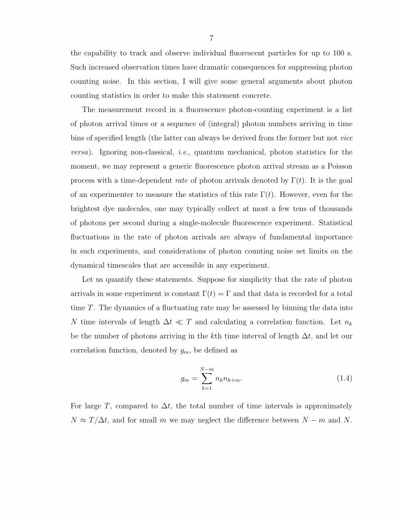
Let us quantify these statements. Suppose for simplicity that the rate of photon

arrivals in some experiment is constant Γ(t) = Γ and that data is recorded for a total

time T . The dynamics of a fluctuating rate may be assessed by binning the data into

N time intervals of length ∆t T and calculating a correlation function. Let nk

be the number of photons arriving in the kth time interval of length ∆t, and let our

correlation function, denoted by gm, be defined as

gm =N−m∑k=1

nknk+m. (1.4)

For large T , compared to ∆t, the total number of time intervals is approximately

N ≈ T/∆t, and for small m we may neglect the difference between N −m and N .

8

Using basic Poisson properties (E[·] denotes an expectation value)

E[nk] = Γ∆t (1.5a)

E[njnk] =

(Γ∆t)2 , j 6= k

(Γ∆t)2 + Γ∆t , j = k(1.5b)

we find the average value of the correlation function

E [gm] ≈ NΓ∆t = Γ2T∆t , (m 6= 0), (1.6)

while the variance in gm is found to be

E[g2m]− E[gm]2 = Γ2T∆t(1 + 2Γ∆t) , (m 6= 0). (1.7)

The signal-to-noise ratio for resolving this correlation function is therefore given by

SNR =E[gm]√

E[g2m]− E[gm]2

=

√Γ2T∆t

1 + 2Γ∆t. (1.8)

It is important to note that Eq. (1.8) is only valid for ∆t smaller than T , and in fact

it is not even sensible to calculate a correlation function with a time resolution ∆t

larger than the entire measurement interval. Although it is somewhat loose as ∆t

approaches T , let us take Eq. (1.8) together with the ansatz that ∆t < T/2 is the

signal-to-noise ratio for a fluorescence correlation measurement.

SNR is plotted in Fig. 1.4 for Γ = 5000 s−1 (a typical value for a fluorescent

protein), as a function of the time resolution ∆t for three different values of the

observation time T . Note that T = 0.01 s is a typical diffusion time for a biologi-

cal molecule through a diffraction-limited laser focus, while the closed-loop tracking

methods described in this thesis are capable of achieving T = 100 s or greater.

A few features of SNR given by Eq. (1.8) deserve mention. For small bin times

9

10−8

10−6

10−4

10−2

100

10210

0

101

102

103

∆t [s]

SN

R

T = 0.01 sT = 1 sT = 100 s

Figure 1.4: Signal-to-noise ratio SNR of the autocorrelation of a Poisson processgiven by Eq. 1.8. The photon arrival rate was taken to be Γ = 5000 s−1, a mod-est fluorescence count rate achievable with dye molecules or intrinsically fluorescentproteins.

∆t, the signal-to-noise ratio is approximately given by

SNR ≈ Γ√T∆t , Γ∆t 1. (1.9)

At fixed count rate Γ, this expression depends only on the product T∆t so that a

decrease in the timescale ∆t requires a proportional increase in T to maintain the same

signal-to-noise ratio; conversely, an order of magnitude improvement in observation

time leads directly to an order of magnitude improvement in time resolution (at short

timescales). On the contrary, for long bin times, the signal-to-noise ratio is given by

SNR ≈√

ΓT

2, Γ∆t 1, (1.10)

independent of ∆t. As mentioned above, the largest measurable timescale ∆t is pro-

portional to T (we took ∆t < T/2 above), so that again an increase in observation

time T leads to a proportional increase in accessible time intervals ∆t (now at long

timescales). These improvements in the observation time of a single particle drasti-

10

cally improve the experimentally resolvable dynamic regime, both at small and large

timescales ∆t. For the 4 orders of magnitude improvement in T shown in Fig. 1.4,

we gain 8 orders of magnitude in experimentally accessible dynamical regimes (4

orders of magnitude towards each of the large and small ∆t sides). It is precisely

this massive improvement in dynamical resolution that motivates the development

of single-particle tracking methods. These methods may one day provide paradigm-

shifting alterations in the accessible dynamic regimes of single-molecule fluorescence

experiments.

1.4 Context and relation to other work

From the arguments in Sects. 1.2 and 1.3, we see that locking a fluorescent particle to

the focus of a fluorescence microscope enables a number of new experimental advan-

tages. First, the particle’s stochastic motion becomes decoupled from its fluorescence

fluctuations, and second, increased observation times provide significantly enhanced

signal-to-noise ratios over a broad range of timescales. These are the primary moti-

vations for developing the experimental and theoretical techniques presented in this

thesis. Of course, we are not the only people working in this new field, and the work

of a few other groups deserves mention here. Some of these provided motivation for

the present work, while others represent concurrent research that complements the

results described here.

An early and seminal application of feedback control applied to biological physics

came 35 years ago with Howard Berg’s apparatus for holding a swimming bacterium

in the focus of an optical microscope using a six-channel photodetector and a home-

made electromechanical actuator [10]. His paper is enjoyable to read, and the dra-

matic achievements of his feedback controller are evident: “The scene through the

[microscope’s] binocular is extraordinary” he writes. Without explicitly referencing

them, Berg describes about many of the control-theoretic considerations considered in

this thesis: control loop design, feedback bandwidth, signal-to-noise ratio, oscillation,

and instability. In an amusing final comment, he even laments the difficulty of storing

11

and processing the copious amounts of data that can be generated in a locked exper-

imental apparatus. Though data storage technology has changed substantially since

1971, this problem has no doubt cropped up for anyone who has closed a feedback

loop and fully automated an experiment.

More recently, in 1997, Ha et al. built a computer-controlled apparatus for locating

and locking onto the position of an individual dye-labeled DNA molecule bound

to a glass cover slip [11]. Their method involved a rather complicated search-and-

optimization algorithm used to locate and lock immobilized particles with typical rise-

times of 200 ms, corresponding to a feedback bandwidth of approximately 1/2π×(200

ms)−1 = 0.8 Hz at fluorescent count rates of a few tens of kHz.

In 2000, Enderlein published a single-molecule (two-dimensional) tracking pro-

posal in which he introduced the use of a spatially modulated excitation intensity

to encode a particle’s position in a high frequency component of the fluorescence

signal [12]. He proposed to rotate the excitation laser (with Gaussian beam waist

w) in a circular pattern at a radius r and intuited that good performance could be

achieved for r/w = 0.6. (In Chapter 4, I will show that optimal localization is in

fact achieved for r/w = 1/√

2 ≈ 0.7.) Furthermore, he used Monte Carlo simulations

to investigate particle escape probabilities. In another 2000 paper, Enderlein used

his simulations to explore the fluorescence fluctuations arising during such a tracking

experiment [13]. To my knowledge, that paper is the only work other than my own

to discuss closed-loop fluorescence correlation spectroscopy. The analytical results

presented in Chapter 5 thoroughly characterize these statistics and constitute an im-

portant part of this thesis. In a subsequent theoretical study, Andersson [14] studied

the use of nonlinear signal processing and control for three-dimensional fluorescent

particle tracking. In 2002, Decca et al., demonstrated a technique for localizing test

objects driven with computer control by rotating a near-field scanning probe [15].

Significantly, in a series of papers beginning in October 2003, the group of E. Grat-

ton developed a version of Enderlein’s proposal, modified for both two- and three-

dimensional geometry [16–19]. They demonstrated the ability to track bright, slowly

moving objects with high spatial accuracy and performed biological measurements of

12

chromatin dynamics in a cellular environment using these techniques. Another recent

contribution to the field has come from H. Yang’s group, in which near-infrared scat-

tering from metallic particles was used to track their three-dimensional motion [20]

while fluorescence in the visible range was recorded. They do not use any modula-

tion techniques, but rather derive their position sensitivity using quadrant avalanche

photodiodes and DC signal levels. Furthermore, they have derived and simulated

change-point detection algorithms for searching a tracking trajectory and identifying

changes in the diffusion coefficient [21].

Finally, the Anti-Brownian Electrophoretic “ABEL” trap developed by Adam

Cohen and W. E. Moerner deserves mention as a creative and important component of

today’s literature in the field of single-particle closed-loop control [22–24]. They detect

the position of a fluorescent object using either CCD cameras or spatial modulation

techniques and trap the object using voltage-actuated fluidic forces.

My own contributions to this field began in December 2003 when (unaware of

the concurrent work in Gratton’s group) Hideo and I submitted our paper “Feedback

controller design for tracking a single fluorescent molecule” to Applied Physics B, in

many ways as a follow-up to Enderlein’s 2000 paper in the same journal. In that work,

presented in Ch. 2, we considered a realistic plant transfer function as a component

of the particle tracking apparatus. We designed an optimal control law using LQG

methods, and performed extensive numerical simulations based on this control law.

The simulations showed that such methods were more than sufficient for tracking

relatively dim and fast moving particles.

Since then, my work has been focused on the tracking problem with experimen-

tal success first announced in an Optics Express paper published in 2005 [25]. That

paper contains the skeletal beginnings of the theory of closed-loop particle tracking

and correlation spectroscopy presented in full detail in Ch. 5. From there, I devel-

oped a simple framework for calculating noise figures based on photon counting noise

and derived the representation of a tracked particle by Ornstein-Uhlenbeck diffusion

statistics using a Kalman filter, which was published in Applied Physics B in 2006

[26]. These results also lay to rest the notion that complex signal processing (for

13

example, dedicated fast Fourier transform hardware or nonlinear computation) is re-

quired for extracting the frequency components of a rate-modulated stream of photon

pulses. In 2005, Kevin McHale began working full time on the experiment. Together,

we made marked improvements in signal processing and overall experimental stabil-

ity culminating in June 2006 when much of the data presented chapters 7 and 8 was

collected, and submitted as Refs. [27, 28].

It is now an exciting time to work in this new field of closed-loop particle control.

Only a few groups have yet contributed to this budding field, and the landscape is

ripe for rapid technological and concomitant scientific progress. In this light, it is of

primary importance to develop a consistent theoretical framework and vocabulary for

discussing these new techniques. When fluorescence correlation spectroscopy (FCS)

was introduced by Magde, Elson, and Webb in 1972 [6–9], their elegant statistical

description of the technique was just as important as the experimental methods. In

fact, it is my belief that their tidy theoretical framework and the resulting simplicity

of experimental interpretation has led to the explosion of applications of FCS over the

intervening decades. Although the new techniques of particle trapping and tracking

are feedback control problems, very little of the substantial theoretical apparatus of

control theory has been applied in this field. In fact, many of the papers mentioned

above do not even use the word “feedback” in reference to their experimental tech-

nique. I consider the establishment of a control-theoretic language for closed-loop

particle tracking and the demonstration of its quantitative predictive power to be my

ongoing contribution to this field.

1.5 Publications from graduate work

The following is a list of publications based at least in part on my work as a graduate

student in the Mabuchi lab [1–4, 25–29]. Those denoted by (*) are primary topics of

this thesis. Available preprints and reprints can be found online at

http://minty.caltech.edu/papers.

1. Andrew J. Berglund, Andrew C. Doherty, and Hideo Mabuchi, “Photon statis-

http://minty.caltech.edu/papers.php

14

tics and dynamics of Fluorescence Resonance Energy Transfer,” Phys. Rev.

Lett. 89, 068101 (2002).

2. *Andrew J. Berglund and Hideo Mabuchi, “Feedback controller design for track-

ing a single fluorescent molecule,” Appl. Phys. B 78, 653-659 (2004).

3. Kevin McHale, Andrew J. Berglund, and Hideo Mabuchi, “Bayesian estimation

for species identification in single-molecule spectroscopy,” Biophys. J. 86, 3409-

3422 (2004).

4. Andrew J. Berglund, “Nonexponential statistics of fluorescence photobleach-

ing,” J. Chem. Phys. 121, 2899-2903 (2004).

5. *Andrew J. Berglund and Hideo Mabuchi, “Tracking-FCS: Fluorescence corre-

lation spectroscopy of individual particles,” Opt. Express 13, 8069-8082 (2005).

6. *Andrew J. Berglund and Hideo Mabuchi, “Performance bounds on single-

particle tracking by fluorescence modulation,” Appl. Phys. B 83, 127-133

(2006).

7. Kevin McHale, Andrew J. Berglund, and Hideo Mabuchi, “Near-optimal di-

lute concentration estimation via single-molecule spectroscopy,” in preparation,

(2006).

8. *Andrew J. Berglund, Kevin McHale, and Hideo Mabuchi, “Feedback localiza-

tion of freely diffusing fluorescent particles near the optical shot-noise limit,” to

appear in Opt. Lett. (2006).

9. *Andrew J. Berglund, Kevin McHale, and Hideo Mabuchi, “Fast classification

of freely diffusing fluorescent nanoparticles,” in preparation (2006).

15

Part I

Theory

17

Chapter 2

Feasibility Study: LQG ControllerDesign

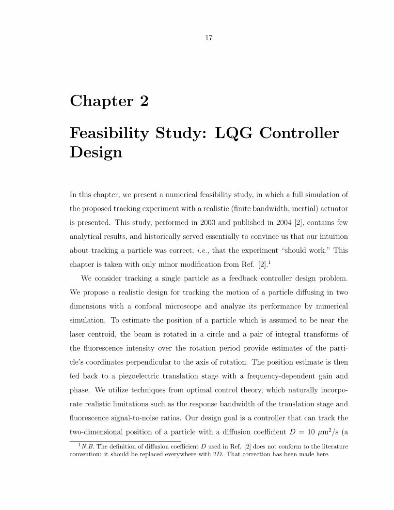
In this chapter, we present a numerical feasibility study, in which a full simulation of

the proposed tracking experiment with a realistic (finite bandwidth, inertial) actuator

is presented. This study, performed in 2003 and published in 2004 [2], contains few

analytical results, and historically served essentially to convince us that our intuition

about tracking a particle was correct, i.e., that the experiment “should work.” This

chapter is taken with only minor modification from Ref. [2].1

We consider tracking a single particle as a feedback controller design problem.

We propose a realistic design for tracking the motion of a particle diffusing in two

dimensions with a confocal microscope and analyze its performance by numerical

simulation. To estimate the position of a particle which is assumed to be near the

laser centroid, the beam is rotated in a circle and a pair of integral transforms of

the fluorescence intensity over the rotation period provide estimates of the parti-

cle’s coordinates perpendicular to the axis of rotation. The position estimate is then

fed back to a piezoelectric translation stage with a frequency-dependent gain and

phase. We utilize techniques from optimal control theory, which naturally incorpo-

rate realistic limitations such as the response bandwidth of the translation stage and

fluorescence signal-to-noise ratios. Our design goal is a controller that can track the

two-dimensional position of a particle with a diffusion coefficient D = 10 µm2/s (a

1N.B. The definition of diffusion coefficient D used in Ref. [2] does not conform to the literatureconvention: it should be replaced everywhere with 2D. That correction has been made here.

18

typical value for a protein in a bilipid membrane) using a commercially available

translation stage. We will show however, that the controller exceeds this criterion by

at least an order of magnitude even for limited motion in a third direction. Further-

more, the values of D which can be tracked are limited by the response bandwidth of

the xy translation stage, so that a faster stage immediately results in faster tracking.

In Sect. 2.1 the state-space formulation of the particle-plus-translation stage sys-

tem is introduced and a procedure for estimating the two-dimensional position of a

fluorescent particle is described. In Sect. 2.2 we treat the system as a target-tracking

problem and present the design of a feedback controller using techniques of optimal

control theory. In Sect. 2.3, we perform numerical simulations of the system over

a wide range of experimental parameters. We indicate the apparent robustness of

this protocol for tracking fast particles with large diffusion coefficients and present

surprising results concerning the ability to track in three dimensions under rather

general conditions.

2.1 State-space dynamics and position estimation

The standard form for a linear, stochastic dynamical system in state-space is

dx = Axdt+ Budt+ dw1 (2.1a)

vdt = Cxdt+ dw2 (2.1b)

where the system state is x(t), the control input is u(t) and the measurement is v(t)

[30]. Stochastic noise is introduced by the white-noise increments dw1 and dw2. In

this section we formulate the dynamics of particle tracking in one dimension in the

form of Eqs. (2.1a-2.1b) when the particle’s position can be directly measured. A

feedback controller then involves the combination of a two-dimensional, fluorescence-

based position estimator (to replace the unattainable direct measurement) with op-

timal feedback strategies based on two copies of the tracking dynamics developed in

this section.

19

101

102

103

−60

−50

−40

−30

−20

−10

0

10

Mag

nitu

de (

dB)

101

102

103

−200

−100

0

100

200

Log Frequency (Hz)

Pha

se (

deg)

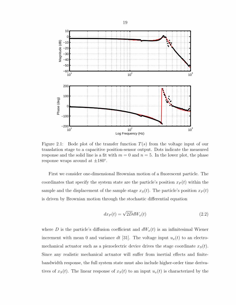
Figure 2.1: Bode plot of the transfer function T (s) from the voltage input of ourtranslation stage to a capacitive position-sensor output. Dots indicate the measuredresponse and the solid line is a fit with m = 0 and n = 5. In the lower plot, the phaseresponse wraps around at ±180.

First we consider one-dimensional Brownian motion of a fluorescent particle. The

coordinates that specify the system state are the particle’s position xP (t) within the

sample and the displacement of the sample stage xS(t). The particle’s position xP (t)

is driven by Brownian motion through the stochastic differential equation

dxP (t) =√

2DdWx(t) (2.2)

where D is the particle’s diffusion coefficient and dWx(t) is an infinitesimal Wiener

increment with mean 0 and variance dt [31]. The voltage input ux(t) to an electro-

mechanical actuator such as a piezoelectric device drives the stage coordinate xS(t).

Since any realistic mechanical actuator will suffer from inertial effects and finite-

bandwidth response, the full system state must also include higher-order time deriva-

tives of xS(t). The linear response of xS(t) to an input ux(t) is characterized by the

20

transfer function T (s) which relates the Laplace transforms XS(s) and Ux(s). (We

will use capital letters to denote the Laplace transform of a function. The complex

argument s of the Laplace transform should not be confused with the subscript index

S, indicating the translation stage coordinates.) For most well-behaved systems, we

may write the transfer function T (s) as

XS(s) = T (s)Ux(s) =p0 + p1s+ · · ·+ pms

m

q0 + q1s+ · · ·+ qn−1sn−1 + snUx(s). (2.3)

The coefficients pj and qj in Eq. (2.3) can be determined by fitting the measured

swept-sine response of the system to an nth order transfer function. We assume

n ≥ m ≥ 1 so the system is proper and non-trivial. Furthermore, we require that the

polynomial in the numerator of Eq. (2.3) has no roots in the right half of the complex

s-plane so that the controller is internally stable. In our experiments, we use a

commercially available piezoelectric translation stage (see Sect. 6.1) whose frequency

response is shown in Fig. 2.1 along with a fit to the data. We find a serviceable fit

with m = 0 and n = 5. If we desire a closer representation of the response around the

resonance at 360 Hz we may always use higher-order fits, so long as they represent

proper, stable systems as defined above. For all of the remaining calculations, we will

use this fit as our plant transfer function T (s).

The inverse Laplace transform of Eq. (2.3) represents an ordinary differential

equation relating xS(t) to ux(t). Taking the control input u(t) to be the highest

relevant time derivative of the input voltage ux(t)

u(t) =dm

dtmux(t) (2.4)

and including xP (t), xS(t) and its first n− 1 derivatives, and ux(t) and its first m− 1

derivatives in the state vector x(t), we may immediately write the matrices A and B

representing the deterministic dynamics in Eq. (2.1a). The stochastic increment dw1

drives xP (t) according to Eq. (2.2) Finally, we consider a noisy (but direct) position

21

measurement

v(t)dt = vx(t)dt = [xP (t)− xS(t)]dt+ σvdWv(t) (2.5)

which defines C and dw2. Finally we let

Σjdt = E[dwjdwTj ] (2.6)

be covariance matrices for j = 1, 2, where E denotes the expectation value over

noise realizations, and T represents the matrix transpose. The state-space dynam-

ical system of Eqs. (2.1a-2.1b) is now fully specified by the diffusion coefficient D,

measurement noise σv, and the coefficients pj and qj.

Some general features of the dynamical system are immediately apparent from the

preceding specification. Along the diagonal, A will naturally partition into blocks of

size 1 × 1, n × n, and m × m corresponding to the dynamics of xP (t), xS(t), and

ux(t) respectively. The coefficients pj fill an off-diagonal block corresponding to the

coupling between xS(t) and ux(t), while xP (t) is not coupled to the other coordinates.

As formulated here, this system is not minimal since it contains the uncontrollable

state xP (t). However, we consider the benefit of using an explicit representation of

all coordinates to outweigh the technical advantages of a minimal formulation. In the

special case m = 0 we simply set u(t) = ux(t) and omit the dimensions of the other

matrices corresponding to the m×m block in A.

For the remainder of this section, we will describe a procedure for approximating

the measurement v(t) of Eq. (2.5) for each of two spatial dimensions. The coordinate

system is shown in Fig. 2.2. The particle’s coordinates are (xP (t), yP (t)) and the

sample stage coordinates are (xS(t), yS(t)), where all coordinates are defined relative

to the origin O, which is fixed in the laboratory frame. We consider a Gaussian laser

beam with beam waist w focused into the plane of Fig. 2.2 and rotating around an

axis normal to the plane and passing through (xS(t), yS(t)). The laser rotates with

a radius r at angular frequency ω0 = 2π/T . We envision an experimental setup in

which the laser is made to rotate using acousto-optic modulators (AOMs), so that

rotation frequencies in the 10 − 50 kHz range are easily obtainable. Defining ΓB as

22

xP(t)

xS(t)

ySyP(t)

r

O

Figure 2.2: Schematic diagram of the coordinates used in the two-dimensional track-ing model of Sect. 2.2. All coordinates are referenced to a fixed origin O in the labframe.

the rate of background photon detections and Γ0 as the rate of fluorescence photon

detections from a particle at the maximum laser intensity, the time-dependent photon

detection rate is given by Γ(t):

Γ(t) = Γ0 exp

[− 2

w2(xP (t)− xS(t)− r cos(ω0t))

2

]× exp

[− 2

w2(yP (t)− yS(t)− r sin(ω0t))

2

]+ ΓB. (2.7)

The actual number of detected photons in any time interval is a Poisson process with

instantaneous rate given by Γ(t).

To find a position estimator, we assume that the particle is close to the laser’s axis

of rotation and that the rotation period T is fast compared to the motion of both

the particle and the stage. Under these assumptions, we may treat the particle’s

coordinates as fixed, and expand Eq. (2.7) to find a linearized count rate Γ(t):

Γ(t) = Γ0 + ΓB +4Γ0

w2(xP − xS) r cos(ω0t) +

4Γ0

w2(yP − yS) r sin(ω0t). (2.8)

23

From Eq. (2.8) we see that within the previous assumptions, good estimates xP and

yP of xP and yP are given by

vx(t) ≡ xP (t)− xS(t) =w2

2r

∫ T

0Γ(t) cos(ω0t)dt∫ T

0Γ(t)dt

(2.9a)

vy(t) ≡ yP (t)− yS(t) =w2

2r

∫ T

0Γ(t) sin(ω0t)dt∫ T

0Γ(t)dt

. (2.9b)

Eqs. (2.9a-2.9b) define the position estimator, which consists only of normalized co-

sine and sine transforms of the measured signal over the rotation period T . These

transforms could be implemented digitally and phase locked with the same signal that

drives the laser rotation, or analog integrations could be performed continuously with

a reset signal phase locked to the laser drive frequency. In either case, the algorithm

gives an estimate vx(t) of xP (t)− xS(t) which corresponds to the measurement term

v(t) in the dynamics of Sect. 2.1.

2.2 Optimal LQG control

In this section, we will apply some standard results from optimal control theory to

estimating the system state x(t) and feeding back to the control inputs. Again, we

will start in one dimension since, aside from the position estimation of Eqs. (2.9a-

2.9b), the x and y dynamics are uncoupled. Furthermore, we will make all of our

arguments in continuous time, relying on the assumption that the period T of the

integral transforms in Eqs. (2.9a-2.9b) is small compared to the diffusion timescale.

All of the following arguments can be formulated in discrete time, but the notation is

simpler in continuous time, and we will see in Sect. 2.3 that the resulting controller

performance justifies this assumption for 1/T ≈ 10 kHz.

We begin with a filter for estimating the full system state x(t) conditioned on the

measurement result v(t). For the one-dimensional case here, v(t) = vx(t) is a scalar.

However, we retain the vector notation to emphasize the generality of the controller

design. We do not know the initial state of the system, but we assume that it is

24

distributed according to a Gaussian distribution with mean m0 and covariance Σ0.

The final form of the controller is largely independent of these initial distributions, so

the choice of m0 and Σ0 is not critical. Since both the system and the measurement

are driven by Gaussian white noise, the optimal probabilistic description of the system

state x(t) remains Gaussian at all times. The equations of motion of the mean m(t)

and covariance Σ(t) of the system state conditioned on the measurement record v(t)

up to time t, can be derived from probabilistic arguments and the result is a Kalman

filter [32, 30]. We simply state these results here:

d

dtm(t) = Am(t) + Bu(t) + Ko(t) [v(t)−Cm(t)] . (2.10)

The observer gain matrix Ko depends on Σ(t)

Ko(t) = Σ(t)CTΣ−12 (2.11)

which propagates according to a non-linear matrix Riccati equation

d

dtΣ(t) = Σ1 + AΣ(t) + Σ(t)AT −Σ(t)CTΣ−1

2 CΣ(t). (2.12)

Note that the Riccati equation for the covariance matrix Σ(t) is deterministic. Since

we are interested in a time-independent form of the estimator, we may numerically

propagate Eq. (2.12) with initial condition Σ(0) = Σ0 to find its steady state solution,

or equivalently we can set the left-hand side to 0 and solve the remaining algebraic

equation numerically (or analytically if possible). Plugging the steady state solution

of Eq. (2.12) into Eq. (2.11) we find the time-independent observer gain matrix Ko.

Having defined an optimal estimate of the system state x(t) conditioned on the

measurements v(t), we now turn to the problem of designing a feedback control signal

u(t) for stabilizing the system state. To this end, we define a “performance criterion”

h(t) which quantifies both the degree to which the system state is stabilized and also

any cost of applying the control signal u(t). In our system, we wish to minimize the

squared tracking error (xP (t)−xS(t))2 while acknowledging that the control signal is

25

a real voltage, limited to finite gain at a finite bandwidth. We therefore penalize the

first time-derivative of the input voltage so that the cost function acknowledges the

bandwidth limitations of a realistic controller. With this in mind, we define matrices

P and Q so that a cost function is given by

h(t) = x(t)TPx(t) + u(t)TQu(t)

= [xP (t)− xS(t)]2 + λ

(d

dtux(t)

)2

(2.13)

where λ is a cost parameter characterizing the bandwidth limitations. The desired

optimal controller is one that minimizes the time integral of h(t). Note that if m = 0,

as is the case for the fit function T (s) of Fig. 2.1, we must augment the system up to

m = 1 so that the control input is ddtux(t) and ux(t) is included in x, with p1 = 0. We

are still guaranteed a proper system because of the non-triviality condition n ≥ 1.

We have now defined a Linear system with a Quadratic performance criterion and

Gaussian noise, an LQG system in the language of optimal control theory [30]. In

such systems, the time-integral of h(t) is minimized by applying the feedback signal

u(t) = −Kcm(t) (2.14)

where the controller gain matrix

Kc = Q−1BTV (2.15)

is again given by the steady-state solution V to a matrix Riccati equation

d

dτV(τ) = P + ATV(τ) + V(τ)A−V(τ)BQ−1BTV(τ) (2.16)

with inital condition V(0) = 0. We use τ and not t as the time argument in Eq. (2.16)

since in an application where we use time varying control [i.e. we do not take the

steady state solutions of Eqs. (2.12) and (2.16)], Eq. (2.16) propagates V backwards

in time with τ representing the time-to-go in the control problem. In the time-

26

independent case, this distinction is irrelevant. Since our system contains an uncon-

trollable state, one component of V diverges as τ →∞ in Eq. (2.16). However, this

component does not enter into the controller gain Kc.

Finally, by inserting the Laplace transform of Eq. (2.14) into the Laplace trans-

form of Eq. (2.10), and rearranging terms we find the overall controller transfer

function relating the control signal U(s) to the measurement V(s):

U(s) = −Gλ(s)V(s)

Gλ(s) = Kc (sI−A + KoC + BKc)−1 Ko. (2.17)

Note that in the one-dimensional tracking case, Gλ(s) = Gλ(s) is a single-input-

single-output controller with input vx and output dm

dtmux. We may immediately write

the desired controller transfer function Hλ(s) from vx(s) to ux(s):

Hλ(s) = s−mGλ(s). (2.18)

For tracking in two dimensions, we simply use a second copy of the controller Hλ(s)

to drive uy using the measurement vy.

In Fig. 2.3, Hλ(s) is plotted for various values of the cost parameter λ. If we have

a controller with large gain at arbitrarily high frequencies, we suspect the optimal

controller transfer function is H(s) = Ω[sT (s)]−1 so that the overall open-loop trans-

fer function H(s)T (s) = Ωs−1 looks like an integrator which exhibits ideal stability

and sensitivity, closing the servo at angular frequency Ω. In Fig. 2.3, we see that

Hλ(s) given by the LQG optimization of Eq. (2.18) better approximates H(s) as λ is

decreased. For any realistic controller, however, Hλ(s) is the optimal approximation

to H(s) in the sense of minimizing the cost function. To find a control algorithm

for an experimental system, we simply decrease λ until the controller can no longer

implement the transfer function Hλ(s), for example due to bandwidth limitations,

finite voltage slew-rates or output saturation. The final choice of λ is therefore a

compromise between steady-state tracking error and the level of aggression a con-

27

0

102

103

104

0

Ph

ase

(d

eg

)

λ = 10 -3

λ = 10 -4

λ = 10 -5

λ = 10 -6

H(s)

Frequency (rad/sec)

-40

-20

20

40

60

80

100

120

Ma

gn

itu

de

(d

B)

-180

-90

90

180

270

360

Figure 2.3: Bode diagrams of the transfer function Hλ(s) of Eq. (2.18) for variousvalues of the cost parameter λ. As λ decreases, Hλ(s) more closely approximates theideal transfer function H(s) (dotted line), with Ω ≈ 103 rad/ms.

troller will tolerate. Finally, we note that in this case an important result of the LQG

optimization procedure is the tailored phase response near the servo closing point,

which minimizes ringing and overshoot in the system’s closed-loop step response.

2.3 Performance analysis

To evaluate the performance of the controller design of Sect. 2.2, we numerically inte-

grate the continuous-time system of equations (2.1a-2.1b) for each of two dimensions.

Using a fluorescence model based on the rate Γ(t) we update the position estimator

of Eqs. (2.9a-2.9b) with period T . Finally, we feedback to the control inputs ux(t)

and uy(t) using the Kalman filter equations (2.10) and the optimal control law given

28

0 100 200 300 400 500 600 700 800 900 1000-10

-5

0

x M(t

) [

µm

]

0 100 200 300 400 500 600 700 800 900 1000-5

0

5

y M(t)

[µ

m]

0 100 200 300 400 500 600 700 800 900 1000-10

-5

0

5

10

u y(t)

[V]

0 100 200 300 400 500 600 700 800 900 10000

100

200

300

400

500

t (ms)

Co

un

ts/m

s

Hλ(s)

No Control

0 100 200 300 400 500 600 700 800 900 1000

0

u x(t)

[V]

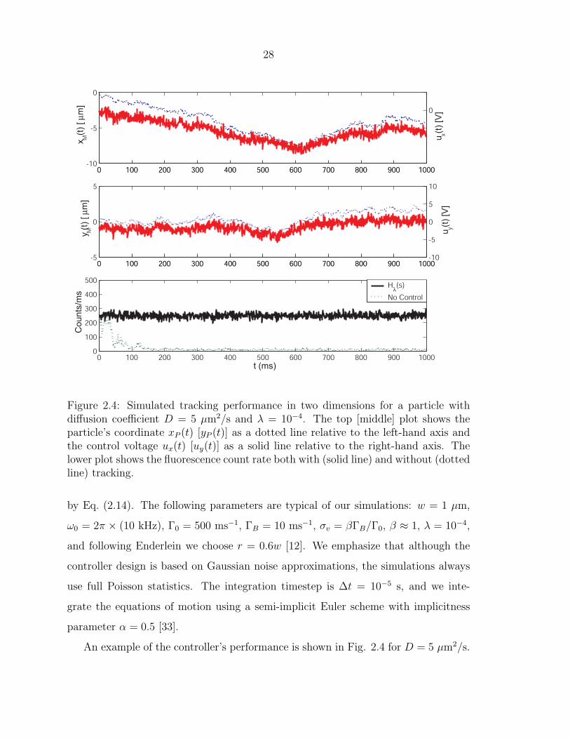
Figure 2.4: Simulated tracking performance in two dimensions for a particle withdiffusion coefficient D = 5 µm2/s and λ = 10−4. The top [middle] plot shows theparticle’s coordinate xP (t) [yP (t)] as a dotted line relative to the left-hand axis andthe control voltage ux(t) [uy(t)] as a solid line relative to the right-hand axis. Thelower plot shows the fluorescence count rate both with (solid line) and without (dottedline) tracking.

by Eq. (2.14). The following parameters are typical of our simulations: w = 1 µm,

ω0 = 2π × (10 kHz), Γ0 = 500 ms−1, ΓB = 10 ms−1, σv = βΓB/Γ0, β ≈ 1, λ = 10−4,

and following Enderlein we choose r = 0.6w [12]. We emphasize that although the

controller design is based on Gaussian noise approximations, the simulations always

use full Poisson statistics. The integration timestep is ∆t = 10−5 s, and we inte-

grate the equations of motion using a semi-implicit Euler scheme with implicitness

parameter α = 0.5 [33].

An example of the controller’s performance is shown in Fig. 2.4 for D = 5 µm2/s.

29

1 10 10010-2

10-1

100

101

102

z = 0 µm

z = 2.5 µm

z = 5 µm

z = 10 µm

No control

D [µm2/s]

Tra

ckin

g e

rror

e τ [µ

m]

Figure 2.5: Log-log plot showing the radial tracking error eτ over a range of diffusioncoefficients and for particles confined to a plane at an axial distance z from thelaser focus. Points which lie a statistically significant distance below the dashed linerepresent regimes in which the controller stabilizes the particle motion.

It is clear that the controller tracks the particle’s position quite well, with fluorescence

fluctuations essentially limited to Poisson statistics. We quantify the performance of

a trajectory over a time τ by the average RMS tracking error

eτ =1

τ

∫ τ

0

[(xP (t)− xS(t))2 + (yP (t)− yS(t))2

] 12 dt. (2.19)

For the trajectory shown in Fig. 2.4, eτ = 0.15 µm, substantially less than the beam

waist w. In fact, the controller exhibits excellent tracking performance with eτ . 0.6

µm for diffusion coefficients up to 50 µm2/s.

Finally, we suspect that the controller will track the radial (xy) motion of particles

diffusing in three dimensions but confined along the z-axis, for example in the case of

particles diffusing between microscope cover slides separated by only a few microns.

For a particle outside of the plane of the laser focus, z = 0, the controller works in

the same way but with z-dependent values of the beam waist w, and the fluorescence

30

intensity Γ0. However, even for incorrect values of these parameters, the position

estimation of Eqs. (2.9a-2.9b) contains information about the direction of a particle’s

motion, while underestimating its displacement. This underestimation is equivalent

to a time-dependent gain variation in the controller Hλ(s). The negative feedback

structure of the controller may provide some robustness, however, and the controller is

still able to track confined three-dimensional motion, albeit with reduced performance

and at a reduced fluorescence intensity.

In Fig. 2.5 we plot eτ for trajectories of length τ = 1 s as D is varied over a

large range of values and for particles confined to a plane at a distance z from the

plane of the laser focus. The solid curve with z = 0 represents tracking performance

for two-dimensional motion while the dashed line represents the untracked case eτ =√

2Dτ . The curves at non-zero z represent the worst-case tracking of a particle

confined to depths between 0 and z. In other simulations, we have seen that the

tracking error is less than those displayed in Fig. 2.5 when the particle is allowed to

move in z instead of being confined to a plane at the maximum depth. All of the

curves show the general feature that the controller stabilizes the tracking error for

diffusion coefficients less than D ≈ 100 µm2/s while above this value, the tracking

error follows the uncontrolled, free-particle diffusion statistics eτ =√

2Dτ . This

value of D represents a fast-moving particle which can escape the rotating laser focus

faster than the response bandwidth of the control system. We estimate this to be

D ≈ πr2νc where νc ≈ 200 Hz is the closing frequency (i.e., unity-gain point) of the

open-loop control system T (s)Hλ(s). We see that while the magnitude of the tracking

error depends on the diffusion coefficient and the depth z, the ability to stabilize the

particle motion depends mainly on the controller bandwidth and the “capture area”

πr2 but is only weakly dependent on z. (All of our simulations have used the value

r = 0.6w with w = 1µm. For a fixed closing bandwidth νc, however, we expect the

controller to track diffusion coefficients which scale as r2 ∼ w2 so that faster particles

can be tracked by simply increasing the focused beam waist w.)

Based on these results, we make the encouraging and perhaps surprising, obser-

vation that the controller can stabilize the radial motion of a moderately fast-moving

31

particle loosely confined to a depth as large as z = 10µm. In this chapter, we did not

attempt a quantitative analysis of the robustness of the controller to gain variation

arising from motion in the uncontrolled z direction. However, well-developed analyt-

ical techniques exist for quantifying system stability and controller performance in

the face of unknown and uncontrolled dynamical plant variation [34, 35], and future

refinements of the controller design presented here could rely on this type of robust-

ness analysis by including a gain variation (position underestimation) with power

spectrum determined by the particle’s diffusion statistics.

33

Chapter 3

Sensing the Position of aFluorescent Particle

Having established the feasibility of closed-loop particle tracking using the realistic

numerical simulations in Ch. 2, we now turn to a more focused investigation of the

problem of detecting a particle’s position using fluorescence modulation and photon

counting. That is, we ask “Why does it work?” The answer, as we shall see, involves

a lot of statistics.

In Ch. 2, we used Eqs. (2.9a-2.9b) to show that the cosine and sine components

of the photon counting rate Γ(t) (at the laser rotation frequency ω0) are proportional

to the particle’s x and y positions, respectively. However, in a real experiment, we do

not measure Γ(t); rather, as shown in Fig. 3.1, we measure a realization of a Poisson

process with that rate. For low fluorescent count rates, it is not immediately obvious

how the frequency components of the rate appear in the frequency components of the

signal itself. To illustrate the problem considered in this section, Fig. 3.1 shows a

time-dependent rate Γ(t) with a strong oscillation at unit frequency together with a

single realization of this process that might be measured in the laboratory.

In our experiment, we rotate the laser at ω0 = 2π×8 kHz, while our average photon

arrival rate is sometimes as low as 5000 s−1. In that case, we collect less than one

photon per rotation period. Furthermore, the electronic signal from our single-photon

counters has a full analog bandwidth of about 500 MHz (the photon counting pulses

have a sub-nanosecond rise time and 25 ns duration), which we demodulate at 8 kHz

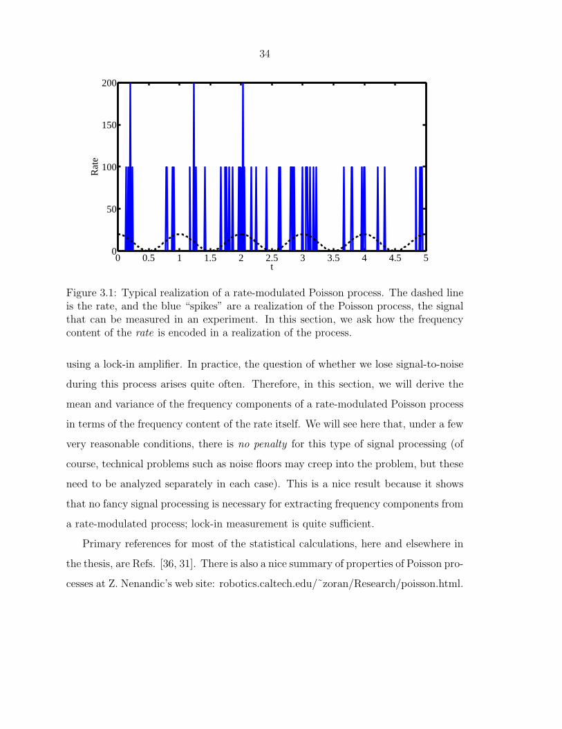
34

0 0.5 1 1.5 2 2.5 3 3.5 4 4.5 50

50

100

150

200

t

Rat

e

Figure 3.1: Typical realization of a rate-modulated Poisson process. The dashed lineis the rate, and the blue “spikes” are a realization of the Poisson process, the signalthat can be measured in an experiment. In this section, we ask how the frequencycontent of the rate is encoded in a realization of the process.

using a lock-in amplifier. In practice, the question of whether we lose signal-to-noise

during this process arises quite often. Therefore, in this section, we will derive the

mean and variance of the frequency components of a rate-modulated Poisson process

in terms of the frequency content of the rate itself. We will see here that, under a few

very reasonable conditions, there is no penalty for this type of signal processing (of

course, technical problems such as noise floors may creep into the problem, but these

need to be analyzed separately in each case). This is a nice result because it shows

that no fancy signal processing is necessary for extracting frequency components from

a rate-modulated process; lock-in measurement is quite sufficient.

Primary references for most of the statistical calculations, here and elsewhere in

the thesis, are Refs. [36, 31]. There is also a nice summary of properties of Poisson pro-

cesses at Z. Nenandic’s web site: robotics.caltech.edu/˜zoran/Research/poisson.html.

http://robotics.caltech.edu/$sim $zoran/Research/poisson.html

35

3.1 Rate-modulated Poisson statistics

Consider a scenario in which an incident photon generates a response function f0(t)

with time-dependent probability Γ(t). In an experiment, f0(t) is an electronic pulse

that signals a single photon detection event and Γ(t) is the time-dependent (mod-

ulated) fluorescence photon counting rate. We may then write f(t), the resulting

stochastic signal, as

f(t) = (f0 ∗ T ) (t) =

∫ ∞

−∞dt′f0(t− t′)T (t′) (3.1)

where ∗ denotes a convolution integral, and the photon detection times tk are recorded

in the stochastic variable T (t)

T (t) =∑

k

δ(t− tk) (3.2)

whose statistics are determined by Γ(t). The next few paragraphs are devoted to a

demonstration of the following results, which will resurface many times:

E [T (t)] = Γ(t) (3.3a)

E [T (t′)T (t′′)] = Γ(t′)Γ(t′′) + Γ(t′)δ(t′ − t′′). (3.3b)

E[·] denotes an expectation value over realization of a process (to be distinguished

from 〈·〉, which we will use to denote a time average in later sections).

We will assume that Γ(t) = 0 for all t outside some bounds |t| > tmax, i.e., that the

signal turns on and off at finite times, so that we need not worry about convergence

of integrals later. Consider the process

Nt = maxtk≤t

k. (3.4)

where Nt is the (stochastic) number of photon arrivals up to time t. It follows imme-

36

diately that

T (t) =d

dtNt

Nt =

∫ t

−∞T (t′)dt′. (3.5)

We have introduced the linear change of variables from T (t) toNt since the probability

distribution over Nt takes on the usual Poisson form. A standard calculation [31]

shows that the probability that Nt takes on the (integer) value n is:

P (Nt = n) =e−λtλn

t

n!(3.6)

where

λt = E [Nt] =

∫ t

−∞Γ(t′)dt′. (3.7)

That is, Nt is just a time-dependent Poisson process with mean value λt.

Now that we know the distribution of Nt, we may calculate the moments of T (t).

First,

E [T (t)] = E[∂

∂tNt

]=

∂

∂tE [Nt] =

∂

∂tλt = Γ(t), (3.8)

which already gives the desired result for Eq. (3.3a). We need to do a little more

work to show Eq. (3.3b). We have

E [T (s)T (t)] = E[∂Ns

∂s

∂Nt

∂t

]=

∂

∂s

∂

∂tE [NsNt] . (3.9)

Using standard properties of Poisson processes, we have for s ≤ t

E [NsNt] = E [Ns(Nt −Ns +Ns)]

= E [Ns(Nt −Ns)] + E[N2

s

]= λs(λt − λs) +

(λ2

s + λs

)= λtλs + λs, (3.10)

37

where we have used the fact that Nt and Nt − Ns are uncorrelated for s ≤ t. In

general, we find

E [NsNt] = λsλt + λmins,t. (3.11)

Taking the partial derivative with respect to t, we find

∂

∂tE [NsNt] = λsΓ(t) , s ≤ t

= λsΓ(t) + Γ(t) , s > t (3.12)

or∂

∂tE [NsNt] = Γ(t)λs + Γ(t)Θ(s− t) (3.13)

where Θ is the Heaviside step function. Now taking the partial with respect to s, we

have the desired result for Eq. (3.3b)

E [T (s)T (t)] =∂

∂s

∂

∂tE [NsNt] = Γ(s)Γ(t) + Γ(t)δ(s− t). (3.14)

3.2 Power spectrum of a rate-modulated Poisson

process

We may now address the primary question, what is the frequency content of the signal

f(t) defined in Eq. (3.1) and how does it depend on the frequency content of the rate

Γ(t)? In other words, how does a wiggle in the excitation laser’s position show up in

the photon counting signal at our detectors?

The complex frequency spectrum of f(t) is given by

F (ω) =

∫ ∞

−∞e−iωtf(t)dt

=

∫ ∞

−∞e−iωt (f0 ∗ T ) (t)

= F0(ω)

∫ ∞

−∞e−iωtT (t)dt (3.15)

38

where F0(ω) is the Fourier transform of the pulse function f0(t). Because T (t) is

stochastic, so is the power spectrum F (ω). Let us calculate some moments of F (ω).

By the linearity of the Fourier transform,

E [F (ω)] = F0(ω)

∫ ∞

−∞e−iωtE [T (t)] dt

= F0(ω)

∫ ∞

−∞e−iωtΓ(t)dt. (3.16)

Defining

Υ(ω) =

∫ ∞

−∞e−iωtΓ(t)dt (3.17)

to be the frequency spectrum of the rate Γ(t), we have

E [F (ω)] = F0(ω)Υ(ω). (3.18)

It is clear that the frequency content of the modulation Γ(t) is contained in the

overall signal, but the amplitude at any frequency is suppressed or enhanced by the

frequency content of the pulse shape F0(ω). In a real experimental scenario we are

more interested in averages over the real and imaginary parts of F (ω) since these

correspond to the cosine and sine transforms in Eq. (2.9a-2.9b).

E Re [F (ω)] = Re E [F (ω)] = Re [F0(ω)Υ(ω)] (3.19)

and similarly for the imaginary part. Note however that a similar relation does not

hold for the magnitude:

E [|F (ω|] 6= |E [F (ω)]|. (3.20)

We may also ask about the fluctuations in the stochastic frequency spectrum F (ω).

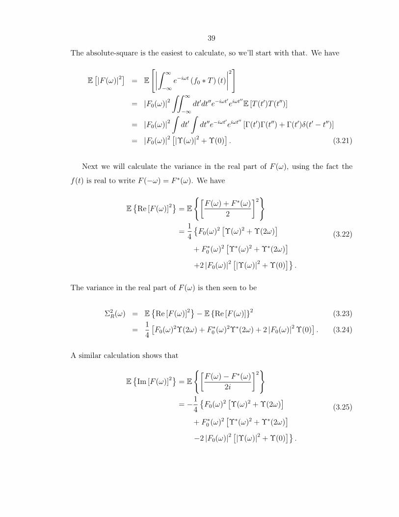
39

The absolute-square is the easiest to calculate, so we’ll start with that. We have

E[|F (ω)|2

]= E

[∣∣∣∣∫ ∞

−∞e−iωt (f0 ∗ T ) (t)

∣∣∣∣2]

= |F0(ω)|2∫∫ ∞

−∞dt′dt′′e−iωt′eiωt′′E [T (t′)T (t′′)]

= |F0(ω)|2∫dt′∫dt′′e−iωt′eiωt′′ [Γ(t′)Γ(t′′) + Γ(t′)δ(t′ − t′′)]

= |F0(ω)|2[|Υ(ω)|2 + Υ(0)

]. (3.21)

Next we will calculate the variance in the real part of F (ω), using the fact the

f(t) is real to write F (−ω) = F ∗(ω). We have

ERe [F (ω)]2

= E

[F (ω) + F ∗(ω)

2

]2

=1

4

F0(ω)2

[Υ(ω)2 + Υ(2ω)

]+ F ∗

0 (ω)2[Υ∗(ω)2 + Υ∗(2ω)

]+2 |F0(ω)|2

[|Υ(ω)|2 + Υ(0)

].

(3.22)

The variance in the real part of F (ω) is then seen to be

Σ2R(ω) = E

Re [F (ω)]2

− E Re [F (ω)]2 (3.23)

=1

4

[F0(ω)2Υ(2ω) + F ∗

0 (ω)2Υ∗(2ω) + 2 |F0(ω)|2 Υ(0)]. (3.24)

A similar calculation shows that

EIm [F (ω)]2

= E

[F (ω)− F ∗(ω)

2i

]2

= −1

4

F0(ω)2

[Υ(ω)2 + Υ(2ω)

]+ F ∗

0 (ω)2[Υ∗(ω)2 + Υ∗(2ω)

]−2 |F0(ω)|2

[|Υ(ω)|2 + Υ(0)

].

(3.25)

40

And the variance in the imaginary part of F (ω) is given by

Σ2I(ω) = −1

4

[F0(ω)2Υ(2ω) + F ∗

0 (ω)2Υ∗(2ω)− 2 |F0(ω)|2 Υ(0)]. (3.26)

Note that Eqs. (3.22) and (3.25) exhibit the general property that

ERe [F (ω)]2

+ E

Im [F (ω)]2

= E

[|F (ω)|2

]. (3.27)

Denoting the signal-to-noise ratio in the real and imaginary parts by (S/N)R and

(S/N)I respectively, we have

(S/N)R =E Re [F (ω)]√

Σ2R(ω)

=

√|F0(ω)|2 |Υ(ω)|2 + Re [F0(ω)2Υ(ω)2]

|F0(ω)|2 Υ(0) + Re [F0(ω)2Υ(2ω)](3.28a)

(S/N)I =E Im [F (ω)]√

Σ2I(ω)

=

√|F0(ω)|2 |Υ(ω)|2 − Re [F0(ω)2Υ(ω)2]

|F0(ω)|2 Υ(0)− Re [F0(ω)2Υ(2ω)]. (3.28b)

These are the desired results, showing the signal-to-noise ratio when the cosine

and sine (real and imaginary) quadratures of a rate-modulated Poisson process are

detected using a lock-in method. Now let us consider detection at a specific mod-

ulation frequency ω0. We assume that our experiment is well-designed, so that

Υ(2ω0) Υ(ω0), i.e., the frequency content of the modulated rate Γ(t) is sharply

peaked at ω0 with a negligible component at the first harmonic frequency 2ω0. Then

we may neglect the second term in both denominators and, denoting the phases of

F0(ω0) and Υ(ω0) by φF0 and φΥ respectively, Eqs. (3.28a-3.28b) become much sim-

pler:

(S/N)R ≈ |Υ(ω0) cos (φΥ + φF0)|√Υ(0)/2

(3.29a)

(S/N)I ≈ |Υ(ω0) sin (φΥ + φF0)|√Υ(0)/2

. (3.29b)

Aside from the phase factor φF0 , which may be eliminated by a suitable choice of

the time origin or equivalently the detection phase, the frequency content of the pulse

41

f0(t) does not contribute to the signal-to-noise ratio. Note that

Υ(0) =

∫ ∞

−∞Γ(t)dt (3.30)

is the average number N of photons collected during the measurement. Not surpris-

ingly, Eqs. (3.29a-3.29b) characteristically scale as 1/√N .

3.3 Application to position sensing

Now that we have established in detail how to calculate the signal-to-noise ratio for

a rate-modulated Poisson process, let us return to more specific considerations of

closed-loop particle tracking. In particular, consider a particle that is immobilized in

the xy plane. In the laboratory, such an immobilized particle is a useful diagnostic for

signal levels, lock-in phases, and tracking error signal quality. In this section, we will

examine some of the shapes that appear when we rotate an excitation laser, focus

it onto an immobilized sample, then plot the two quadrature outputs of a lock-in

measurement on an oscilloscope.

Before going any further, we can get all of the necessary calculations out of the

way in one line. Let p and q be real numbers and let m be an integer. Then consulting

Gradshteyn and Ryzhik [37] formula 3.919, we find

1

2π

∫ 2π

0

exp (p cos θ + q sin θ + imθ) dθ = exp [im arg (p+ iq)] Im

(√p2 + q2

)(3.31)

where Im is the modified Bessel function of order m and arg(z) is the argument (phase

angle) of the complex number z. Essentially every integral that we will require for

the rest of this chapter (and most other chapters too) comes down to Eq. (3.31) with

a suitable choice of p, q, and m.

Now consider the usual Gaussian laser with beam waist w rotating at a radius r at

angular frequency ω0. We will now move into the reference frame of the laser centroid

42

x

ρ

θ

Figure 3.2: Schematic diagram of the coordinates used for the tracking model, in thereference frame of the laser centroid.

and drop the subscript M on the particle’s coordinates as shown in Fig. 3.2. In a

fixed plane z perpendicular to the axis of rotation, the fluorescence photon arrival

rate from a particle at position x = (ρ, θ), given in polar coordinates, is

Γx(t) = Γ0 exp

− 2

w2

[(ρ cos θ − r cosω0t)

2 + (ρ sin θ − r sinω0t)2]

= Γ0 exp

[− 2

w2(r2 + ρ2)

]exp

[4rρ

w2cos(θ − ω0t)

]. (3.32)

The corresponding frequency spectrum will be denoted by Υx(ω) and defined as in

Eq. (3.16).

Now consider making a lock-in detection of the fluorescence signal at the lock-in

frequency ω0. We will denote the expectation values of the cosine and sign quadrature

outputs of this lock-in measurement by x(ρ, θ) and y(ρ, θ), which are special cases of

the frequency spectra defined in Sect. 3.2:

x(ρ, θ) = E Re [Υx(ω0)] =

∫ 2π/ω0

0

Γx(t) cos(ω0t)dt (3.33)

y(ρ, θ) = E Im [Υx(ω0)] =

∫ 2π/ω0

0

Γx(t) sin(ω0t)dt. (3.34)

43

2 0 22

1

0

1

2

x

y

2 0 22

1

0

1

2

2 0 2 2

1

0

1

2

x

y

2 0 2 2

1

0

1

2

2 0 2 2

1

0

1

2

x

y 2 0 2

2

1

0

1

2

x

y

^

^

xy

^^

x

y

^

^

Figure 3.3: Three examples of the mapping defined by equations (3.35) and (3.36).The upper plots show various lines in the (x, y) ↔ (ρ, θ) plane, while the lower plotsshow the resulting curves (x(ρ, θ), y(ρ, θ)) in the (x, y) plane. These lower curves arethe result of a lock-in position estimation measurement for a molecule moving alongthe upper lines, when the resulting quadrature amplitudes are plotted against eachother. The parameters used were Γ0 = ω0, r = 0.5 and w = 1.

Of course, we chose the symbols x and y, because these provide our estimate of the x

and y position of the particle. With some trigonometric identities and formula (3.31),

we find x and y explicitly:

x(ρ, θ) = 2πΓ0

ω0

exp

[− 2

w2

(ρ2 + r2

)]I1

[4rρ

w2

]cos θ (3.35)

y(ρ, θ) = 2πΓ0

ω0

exp

[− 2

w2

(ρ2 + r2

)]I1

[4rρ

w2

]sin θ. (3.36)

This pair of transformations maps lines in the (ρ, θ) plane to curves in the (x, y)

44

plane, with the interesting property that the angular coordinate θ is unchanged. We

may therefore think of it as the radial mapping

h(ρ) = 2πΓ0

ω0

exp

[− 2

w2

(ρ2 + r2

)]I1

[4rρ

w2

](3.37)

such that (ρ, θ) 7→ (h(ρ), θ). In the limit ρ/w 1, with r ∼ w, we have

h(ρ) ≈ 4πrρ

w2exp

[−2

r2

w2

]. (3.38)

The above fact, that h(ρ) ∝ ρ for small ρ, gives the utility of lock-in position estima-

tion in a closed-loop feedback tracking algorithm. In Fig. 3.3, we show some lines in

the (x, y) ↔ (ρ, θ) plane and the resulting curves in the (x, y) plane. In the labora-

tory, if we translate an immobilized particle along the paths shown at the top of Fig.

3.3, the resulting lock-in quadrature outputs plotted in xy mode on an oscilloscope

will resemble the curves shown at the bottom.

3.4 Autocorrelation functions: More statistics!

In addition to plotting lock-in quadrature outputs, it is often useful in the laboratory

to calculate autocorrelation functions of the fluorescence intensity recorded when

an immobilized sample is illuminated with the rotating laser. In this section, we

will calculate various of these autocorrelation functions for the case that one, two,

or a random distribution of many particles are distributed on the surface. These

calculations are a little tedious, but I think it is useful to record them here for exactly

that reason.

We will use the same notation as Sects. 3.1-3.2, where f(t) is a rate-modulated

Poisson process with rate Γx(t) defined by Eq. (3.32). The autocorrelation function

of f(t) is defined to be

C(τ) =

∫ ∞

−∞dtf(t)f(t+ τ). (3.39)

As before, we assume that the signal f(t) turns on and off at finite times, so that the

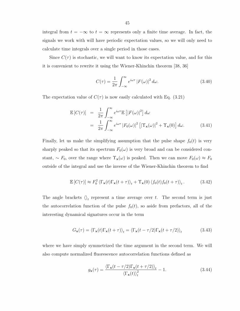
45

integral from t = −∞ to t = ∞ represents only a finite time average. In fact, the

signals we work with will have periodic expectation values, so we will only need to

calculate time integrals over a single period in those cases.

Since C(τ) is stochastic, we will want to know its expectation value, and for this

it is convenient to rewrite it using the Wiener-Khinchin theorem [38, 36]

C(τ) =1

2π

∫ ∞

−∞eiωτ |F (ω)|2 dω. (3.40)

The expectation value of C(τ) is now easily calculated with Eq. (3.21)

E [C(τ)] =1

2π

∫ ∞

−∞eiωτE

[|F (ω)|2

]dω

=1

2π

∫ ∞

−∞eiωτ |F0(ω)|2

[|Υx(ω)|2 + Υx(0)

]dω. (3.41)

Finally, let us make the simplifying assumption that the pulse shape f0(t) is very

sharply peaked so that its spectrum F0(ω) is very broad and can be considered con-

stant, ∼ F0, over the range where Υx(ω) is peaked. Then we can move F0(ω) ≈ F0

outside of the integral and use the inverse of the Wiener-Khinchin theorem to find

E [C(τ)] ≈ F 20 〈Γx(t)Γx(t+ τ)〉t + Υx(0) 〈f0(t)f0(t+ τ)〉t . (3.42)

The angle brackets 〈〉t represent a time average over t. The second term is just

the autocorrelation function of the pulse f0(t), so aside from prefactors, all of the

interesting dynamical signatures occur in the term

Gx(τ) = 〈Γx(t)Γx(t+ τ)〉t = 〈Γx(t− τ/2)Γx(t+ τ/2)〉t (3.43)

where we have simply symmetrized the time argument in the second term. We will

also compute normalized fluorescence autocorrelation functions defined as

gx(τ) =〈Γx(t− τ/2)Γx(t+ τ/2)〉t

〈Γx(t)〉2t− 1. (3.44)

46

Now let us calculate these autocorrelation functions for a few different cases.

Autocorrelation for a single particle. First, consider a single fluorescent particle

immobilized to a two-dimensional surface at position x = (ρ, θ) in a rotating Gaussian

laser. For this case, again with the aid of Eq. (3.31), we find

Gx(τ) = 〈Γx(t− τ/2)Γx(t+ τ/2)〉t

=ω0

2π

∫ 2π/ω0

0

Γx(t− τ/2)Γx(t+ τ/2)dt

= Γ20 exp

[− 4

w2(r2 + ρ2)

]I0

[8rρ

w2cos(ω0τ/2)

](3.45)

where the time average was computed simply as the average over a single period of

the rotation. The normalized autocorrelation gx(τ) for a single molecule in a rotating

laser field is therefore given by

gx(τ) =1

I0 (4rρ/w2)2 I0

[8rρ

w2cos(ω0τ/2)

]− 1. (3.46)

Average autocorrelation for a single particle. We may also compute the av-

erage correlation function G(τ), averaged over uniformly distributed positions x:

G(τ) = 2π

∫ ∞

0

Gx(τ)ρdρ

=Γ2

0w2π

4exp

−4r2

w2

[1− cos2

(ω0τ

2

)]. (3.47)

Cross-correlation for a pair of particles. Letting xj = (ρj, θj) be the position

of particle j, we define the cross-correlation between fluorescence from particles j and

k as follows:

Gxj ,xk(τ) ≡ 〈Γ(ρj, θj, t− τ/2)Γ(ρk, θk, t+ τ/2)〉t

= ξω0

2π

∫ 2π/ω0

0

exp [p cos(ω0t) + q sin(ω0t)] dt (3.48)

47

0 0.5 1 1.5 2 2.5 30

0.5

1

1.5

2

2.5

3

3.5

τ

x = 0.0

x = 0.2

x = 0.4

x = 0.6

x = 0.8

x = 1.0

gx(τ

)

Figure 3.4: gx(τ) as given by Eq. (3.46), for various values of the parameter x =rρ/w2.

where

ξ = Γ20 exp

[− 2

w2

(ρ2

j + ρ2k + 2r2

)](3.49a)

p =4r

w2

[ρj cos

(θj +

ω0τ

2

)+ ρk cos

(θk −

ω0τ

2

)](3.49b)

q =4r

w2

[ρj sin

(θj +

ω0τ

2

)+ ρk sin

(θk −

ω0τ

2

)]. (3.49c)

Using Eq. (3.31), we have

Gxj ,xk(τ) =

Γ20 exp

[− 2

w2

(ρ2

j + ρ2k + 2r2

)]I0

[4r

w2

√ρ2

j + ρ2k + 2ρjρk cos(θj − θk + ω0τ)

].

(3.50)

Note that, unlike the autocorrelation Gx(τ) = Gx,x(τ), Gxj ,xk(τ) is not restricted to

be symmetric around τ = 0, nor is it necessarily a maximum at τ = 0.

48

Because the laser rotates at a fixed radius r, the cross-correlation Gxj ,xk(τ) is

sensitive only to the angular separation between the particles. To see this, we can

integrate Gxj ,xk(τ) over the angular variables θj, θk to find

∫ 2π

0

dθj

2π

∫ 2π

0

dθk

2πGxj ,xk

(τ)

= Γ20 exp

[− 2

w2

(ρ2

j + r2)]I0

(4rρj

w2

)exp

[− 2

w2

(ρ2

k + r2)]I0

(4rρk

w2

)=⟨Γxj

(t)⟩

t〈Γxk

(t)〉t .

(3.51)

In the last line, we see explicitly that there is no radial contribution to the two-

particle cross-correlation. By the way, the following integral was useful for getting to

Eq. (3.51):1

2π

∫ 2π

0

I0

(√α2 + β2 + 2αβ cos θ

)dθ = I0(α)I0(β). (3.52)

Autocorrelation for a distribution of particles. Finally, let us construct the

full two-time fluorescence correlation function from a surface immobilized distribution

of particles characterized by the set of coordinates R = xj. The total intensity is

given by

ΓR(t) =∑xj∈R

Γx(t) (3.53)

and the two-time fluorescence correlation function is given by

GR(τ) = 〈ΓR(t− τ/2)ΓR(t+ τ/2)〉t

=∑j,k 6=j

Gxj ,xk(τ) +

∑j

Gxj(τ). (3.54)

Eq. (3.54) is the exact two-time fluorescence correlation function measured from a

fixed arrangement of particles at positions specified by R. We may now average over

arrangements R to find the result of a trajectory-averaged experimental run. Let

c(x) be the probability density for a particle to be at position x and let c(x1,x2) be

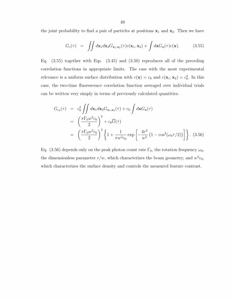
49

the joint probability to find a pair of particles at positions x1 and x2. Then we have

Gc(τ) =

∫∫dx1dx2Gx1,x2(τ)c(x1,x2) +

∫dxGx(τ)c(x). (3.55)

Eq. (3.55) together with Eqs. (3.45) and (3.50) reproduces all of the preceding

correlation functions in appropriate limits. The case with the most experimental

relevance is a uniform surface distribution with c(x) = c0 and c(x1,x2) = c20. In this

case, the two-time fluorescence correlation function averaged over individual trials

can be written very simply in terms of previously calculated quantities.

Gc0(τ) = c20

∫∫dx1dx2Gx1,x2(τ) + c0

∫dxGx(τ)

=

(πΓ0w

2c02

)2

+ c0G(τ)

=

(πΓ0w

2c02

)21 +

1

πw2c0exp

[−4r2

w2

(1− cos2(ω0τ/2)

)]. (3.56)

Eq. (3.56) depends only on the peak photon count rate Γ0, the rotation frequency ω0,

the dimensionless parameter r/w, which characterizes the beam geometry, and w2c0,

which characterizes the surface density and controls the measured feature contrast.

51

Chapter 4

Tracking Limits: Photon CountingNoise

In Ch. 3, we considered in detail the statistics of position sensing based on fluorescence

modulation for static particles. In this chapter, we move to the dynamic regime by

allowing the particle to move by Brownian motion during the position sensing process.

In particular, we ask, “How well can we track a Brownian particle using fluorescence

modulation?” We will now bring notions from control theory into our analysis, draw-

ing strongly on the Kalman filter [30]. The fundamental limit on the localization will

depend on the number of photons collected during the characteristic particle tracking

time, i.e., the feedback bandwidth. Everything in this chapter is theoretical, but in

Ch. 8, we will show how close we come in practice to the fundamental limits derived

here. This chapter is taken with minor modification from Ref. [26].

Because of the Poisson statistics of fluorescence detection, the experimental signal

in our tracking experiment is fundamentally noisy. As a result, any estimate of the

particle’s position based on this signal also inherits this noise. For a static particle,

this uncorrelated noise can be removed by sufficient temporal averaging (both for

imaging and non-imaging techniques), a fact exploited by Yildiz et al. to achieve

nanometer fluorescent particle localization [39]. However, if a particle moves during

the measurement, either stochastically or in an unknown deterministic way, the fluo-

rescence noise results in a fundamental limit on the accuracy with which its position

can be determined. Roughly speaking, a fast particle cannot be localized as accu-

52

rately as a slow particle. In tracking applications, if a particle cannot be sufficiently

localized within the characteristic tracking timescale, then it cannot be tracked at all.

In this chapter, we consider these fundamental constraints, and we place upper limits

on the performance of particle tracking by fluorescence modulation in the presence of

photon counting noise. We do not consider the finite bandwidth response of a realistic

actuator; here, we only consider tracking performance limits based on photon count-

ing statistics. In Sect. 4.1, we derive a simple expression for the noise spectral density

in a fluorescence modulation measurement using the statistics developed in Ch. 3. In

Sect. 4.2, we consider the statistical task of estimating a moving particle’s position

by filtering a noisy measurement. In Sect. 4.4, we present the results of numerical

simulations of the tracking process, including in the nonlinear regime where some of

our approximations break down, and give a qualitative method for determining the

parameter regimes in which a particle can be tracked.

4.1 Static position estimation

In this section, we are concerned with estimating the position of a static particle

using fluorescence modulation and demodulation techniques. We will derive results

for our own quasi-two-dimensional tracking geometry, but the arguments generalize

in a straightforward way to different experimental geometries. The definitions and

notation are similar to preceding chapters, but not identical so we will reintroduce

everything briefly here. We still consider a particle’s two-dimensional position in the

xy ↔ ρθ plane as shown in Fig. 3.2. The rate of fluorescence from a particle at

position x = (x, y) ↔ (ρ, θ) is given by

Γx(t) = Γ0 exp

−2

[ρ2

w2+r2

w2− 2

rρ

w2cos (θ − ω0t)

](4.1)

where Γ0 is the peak fluorescence rate, w is the beam waist, r is the radius of rotation

of the beam, and ω0 is the angular rotation frequency.

As discussed previously, the measured fluorescence signal is a stochastic train of

53

voltage pulses from the output of a single-photon counter, with the arrival times of

the pulses governed by the rate Γx(t). Letting V (t) denote the shape of the electronic

pulses, the full stochastic fluorescence signal s(t) is given by a convolution integral

s(t) = (T ∗ V ) (t) ≡∫ ∞

−∞V (t− t′)T (t′)dt′ (4.2)

where T (t) is defined as in Eq. (3.2).

In order to estimate the particle’s position x, we must extract the component of

s(t) [actually the component of Γx(t)] at the laser rotation frequency ω0, a statistical

task we have already discussed in detail in Ch. 3. We assume that ω0 is much faster

than the timescale of the particle’s motion, so that over a single rotation period

the particle can be considered to be stationary. Furthermore, we assume that the

voltage pulses are very narrow (in time) compared to all other frequencies of interest,

so that we may write V (t) ≈ V0δ(t) or equivalently s(t) ≈ V0T (t).1 We define the

“instantaneous” component of s(t) at angular frequency ω to be

st(ω) =

∫ t+2π/ω0

t

e−iωts(t)dt

≈ V0

∫ t+2π/ω0

t

e−iωtT (t)dt ≡ V0Tt(ω) (4.3)

where Tt(ω) is the finite-windowed Fourier transform of T (t), over one rotation pe-

riod 2π/ω0 beginning at time t. The real and imaginary parts of st(ω), or at least

a bandwidth-limited filtration of these components, can be measured using phase-

sensitive lock-in detection. These measurements probe a time-dependent, stochastic

frequency spectrum st(ω). The expectation value of the component of s(t) at nω0,

where n is a positive integer, is given by [cf. Eqs. (3.3a)-(3.3b) and (3.31)]:

E[st(nω0)] = V0E[Tt(nω0)

]= V0hn (ρ) einθ (4.4)

1For our experiments, we use avalanche photodiodes with a pulse width of approximately 25 ns,while the rotation period is 125 µs, so this approximation is quite valid.

54

with

hn(ρ) = 2πΓ0

ω0

exp

[− 2

w2

(r2 + ρ2

)]In

(4rρ

w2

). (4.5)

In is the nth-order modified Bessel function. For ρ/w 1 and ρr/w2 1 (we will

further assume that r ∼ w), we may write

hn(ρ) ≈ 2π

n!

(Γ0

ω0

)(2ρr

w2

)n

exp

[−2

r2

w2

]+O

( ρw

)n+1

. (4.6)

For n = 1, Eq. (4.6) for h1(ρ) shows that the component of s(t) at frequency ω0 is,

on average, linear in the radial coordinate ρ near the origin. Information about the

angular coordinate θ is contained in the complex exponential phase, whose real and

imaginary parts are accessible by lock-in detection. Near the origin, the real part of

st(ω0) is linear in the particle’s x coordinate and the imaginary part is linear in the y

component (on average). This linear dependence of the mean values of st(ω0) near the

origin provides the error signal for lock-in detection. Furthermore, the time-averaged

fluorescence intensity is given by the n = 0 component, st(0) while the variance will

be shown to depend on the n = 2 component.

We may now construct an explicit estimator of the (stationary) particle’s x posi-

tion based on the measured frequency component st(ω0). An analogous argument will

hold for the y component. Note that measurement noise results in a time-dependent

position estimate even for a stationary particle, so we must continue to use the sub-

script t. Let us define a reciprocal distance kx by

kx = 4π

(Γ0

ω0

)( r

w2

)exp

[−2

r2

w2

](4.7)

and a stochastic, time-dependent estimate xt of the particle’s position x by

xt =2πB

V0kxω0

Re

∫ t+1/B

t

e−iω0ts(t)dt. (4.8)

In Eq. (4.8), B is the filter bandwidth, which is assumed to be much larger than

the rotation frequency ω0/2π; with this separation of timescales, we may make the

55

-4 -3 -2 -1 0 1 2 3 4-0.25

-0.2

-0.15

-0.1

-0.05

0

0.05

0.1

0.15

0.2

0.25

x

E[x

t]^

Error signal

Fluorescence

Intensity

Figure 4.1: Expectation value E [xt] of the estimator xt (arbitrary units) for r/w = 0.5(blue ) and r/w = 1.5 (red +). The dotted lines are the linear approximation of Eq.(4.6), while the dashed lines show the time-average laser intensity in arbitrary units.

approximation ω0/2πB ≈ N where N is a (large) integer. xt has the desired property

that

E[xt] =2w

r2exp

[−2ρ2

w2

]I1

(4rρ

w2

)≈ ρ cos θ. (4.9)

The approximation is valid near the origin, which is why it is useful as an error

signal for locking the particle’s position to the origin using feedback control. The

expectation value of the estimator E [xt] is shown in Fig. 4.1 for two values of the

offset parameter r/w.

We can now derive the primary result of this section. We may find the the estima-

tor variance, or squared tracking error, xt by plugging in to the preceeding formulas

to find

E[(x− xt)2] =

1

2Nk2x

[h0(ρ) + h2(ρ) cos θ] ≈ h0(ρ)

2Nk2x

(4.10)

where the approximation is valid in the linear regime near the origin. The rightmost

expression in Eq. (4.10) does not depend on ρ, since h0(ρ) also does not, so plugging

56

back in for N and h0(ρ), we find

E[(x− xt)

2]

=

[wψ( rw

)√B

Γ0

]2

, ψ(x) =1√8

ex2

x(4.11)

where ψ is a dimensionless function characterizing the beam geometry. The standard

deviation in the tracking error scales as√B, a characteristic feature of shot noise

processes. The measurement noise density nm arising from photon counting statistics

is given by

nm =

√E [(x− xt)2]√

B= ψ

( rw

) w√Γ0

(4.12)

which has dimensions of (for example) µm/√

Hz. This noise spectral density is valid

for feedback bandwidths B that are large compared to the rotation frequency ω0.

However, note that ω0 appears nowhere within the expression for nm so that we

are free to make ω0 arbitrarily large with no effect on the noise figure. Also, note

that a similar noise figure will apply to noise in the measurement of each Cartesian

component of the particle’s position (for the case described here, the noise figures for

x and y detection are identical).

The specific form of ψ(x) was derived for our particular experimental geometry.

For this case, ψ(r/w) achieves its minimum value at r/w = 1/√

2 where ψ(1/√

2) =

ψopt ≈ 0.82. Recall that the expression for the noise density is only valid in the linear

regime ρ/w 1 together with the additional assumption that r ∼ w, but ψopt is

accessible well within this regime.

If we add a finite background count rate Γb to Γx(t) and carry out the same

analysis, we find a measurement noise density nm →√n2

m + n2b where the background

contribution to the measurement noise density is

nb = ψ

(√2r

w

)w

√2Γb

Γ20

. (4.13)

Finally, note that the results derived here require only the linear relationship between

the frequency components of s(t) and the particle’s position near the origin, which is

57

0 100 200 300 400 500−0.5

−0.4

−0.3

−0.2

−0.1

0

0.1

0.2

0.3

0.4

0.5

Time [B−1

]

Est

imat

ed p

osi

tion [µ

m]

0 10 20−0.5

−0.4

−0.3

−0.2

−0.1

0

0.1

0.2

0.3

0.4

0.5

Figure 4.2: (Left) Numerical simulation of the estimate xt of a particle’s positionbased on fluorescence demodulation. The particle was fixed at the coordinate origin.The red, more localized results are for r/w = 1/

√2, w = 1 µm, Γ0 = 105 s−1, and

ΓB = 0. The blue, wider distribution was computed with r/w = 1.4, Γ0 = 105 s−1,ΓB = 104 s−1. For both curves, the laser rotation period was ω0 = 2π × 8 kHz andthe bandwidth was B = 100 Hz. (Right) Simulated distributions together with thosepredicted by nm

√B as calculated in the text.

an essential ingredient for linearizing and locking a nonlinear system using feedback

control. For a different experimental geometry, or tracking in higher dimensions,

these methods can be applied in exactly the same way to derive the measurement

noise spectral density nm for each Cartesian coordinate. A simulation of the position

estimator xt applied to a stationary particle at the coordinate origin is shown in

Fig. 4.2.

4.2 Dynamic position estimation

In Sect. 4.1, we derived a noise spectral density nm by considering the effect of photon

counting statistics on fluorescence demodulation measurements. This noise density

determines the standard deviation in estimating a static particle’s position in a time

1/B to be nm

√B: a static particle can be localized arbitrarily well by averaging

58

101

102

103

104

10−4

10−3

10−2

10−1

100

Bandwidth [ Hz ]

Tra

ckin

g V

ari

an

ce [

µm

2 ]

Figure 4.3: Mean-square tracking error E[e2t ] as a function of bandwidth B as pre-dicted by Eq. (4.16) for D = 1 µm2/s and the noise spectral density ranging fromnm = 10−2 to nm = 10−3 µm/

√Hz. The solid arrow indicates the direction of de-

creasing nm. The solid black line is the zero-noise limit where the tracking error isD/B and the dashed line is the locus of minima in the tracking error given by Eqs.(4.18a-4.18b).

the measurement for a sufficiently long time. In this section, we will take the noise

spectral density nm as given and consider dynamic position estimation of a diffusing

particle. For this case, there exists an optimal bandwidth and a finite lower bound

on the noise in the particle’s estimated position. In the first part of this section,

we will calculate the localization noise for a first-order low-pass filtration of a diffus-

ing particle’s position plus measurement noise. We will find the optimal bandwidth

and minimum localization noise for this case. We will discuss particle position es-

timation and particle tracking control interchangeably, since we are interested here

in fundamental tracking limits where we assume that the tracking control apparatus

can respond instantaneously to the optimal estimate.2 Therefore, optimal estimation

results are equivalent to optimal control results for this idealized case.

2This not an unattainable experimental scenario if a particle is tracked, for example, by translat-ing an excitation laser using acousto-optic modulators whose response bandwidth may exceed theparticle’s motional timescale by several orders of magnitude.

59

Consider the time-dependent position Xt of a particle diffusing in one dimension

with diffusion coefficient D. If we measure this particle’s position with noise nm, then

form our estimate Xt of the particle’s position by filtering the result at a bandwidth

B, we find the following coupled stochastic differential equations for Xt and Xt

d

Xt

Xt

=

0 0

−B B

Xt

Xt

dt+

√2D 0

0 nmB

dW1

dW2

(4.14)

where dW1 and dW2 are independent stochastic Wiener increments [31] driving the

particle’s diffusion and the measurement noise, respectively. Eq. (4.14) represents a

two-dimensional Ornstein-Uhlenbeck process where the components have an obvious

interpretation in terms of the particle’s position and the estimated position. Since the

Ornstein-Uhlenbeck process is Gaussian, the particle’s position will remain Gaussian

distributed so long as its initial position is either deterministic or Gaussian distributed

as well. We may collapse Eq. (4.14) to a single equation for the measurement error

et = Xt − Xt:

det = −Betdt+√

2DdW , D = D +n2

mB2

2, (4.15)

which is a simple one-dimensional Ornstein-Uhlenbeck process with effective diffusion

coefficient D. Eq. (4.15) suggests that a particle tracked at bandwidth B looks (sta-

tistically) like a freely diffusing particle tracked with no measurement noise, but with

an effectively larger diffusion coefficient D given by the sum of D and the contribution

from measurement noise n2mB

2/2.

We are interested in steady-state tracking, not transient behavior during the lock-

ing process, so we will use steady-state solutions. For long times compared to the

feedback timescale 1/B, we find E[et] = 0 and

E[e2t]

=D

B=D

B+n2

mB

2. (4.16)

60

The steady-state time-correlation function is

G(τ) = limt→∞

E [et+τet] =D

Bexp (−Bτ) (4.17)

which may prove to be useful result for performing fluorescence correlation spec-

troscopy (FCS) while tracking a single particle [25]. Eq. (4.16) gives an asymptotic

limit for particle localization with a simple first-order filtration of the demodulated

fluorescence signal. The optimal bandwidth and estimator variance are given by

Bopt =√

2D/nm (4.18a)

E[e2t]opt

=√

2Dnm. (4.18b)

In Sect. 4.3, the same optimal bandwidth and localization are found by applying

a Kalman filter to the system consisting of the particle’s position Xt and a noisy

measurement of that position. Since the Kalman filter is optimal in the mean-square

sense, that analysis shows that the simple first-order filtration at bandwidth B is in

fact the optimal control law when the experimental response time is not a limiting

factor.

Now suppose we wish to track a particle’s position and we require a squared

tracking error (in the x direction) less than some value σ2x. The maximum diffusion

coefficient Dmax for which a particle can be tracked within this tracking error con-

straint can be found by setting Eq. (4.18b) equal to σ2x and using the full expression

for the measurement noise nm including a finite background:

Dmax =

(Γ0σ

4x

2w2

)ψ ( rw

)2

+ 2Γb

Γ0

ψ

(√2r

w

)2−1

. (4.19)

Eq. (4.19) is an explicit expression for the largest diffusion coefficient Dmax that can

be tracked (in one dimension only) by fluorescence modulation; solving for σx, we find

an expression for the smallest position variance that can be achieved when tracking

a given diffusion coefficient. Note that at fixed r/w, Dmax strictly decreases with

61

D σ(d = 2) σ(d = 3)0.001 14 180.01 26 310.1 45 551.0 81 9910.0 143 175100.0 255 310

Table 4.1: Table showing the best possible standard deviation σ [nm] in localizinga particle with diffusion coefficient D [µm2/s] ranging over relevant values for single-molecule spectroscopy in d = 2 or 3 dimensions. The remaining parameters werefixed at w = 0.5µm, r = w/

√2, Γ0 = 50 kHz, Γb = 10 kHz.

increasing beam waist w; however, at fixed fractional localization σx/w, Dmax strictly

increases with w.

Now consider tracking isotropic diffusion in 3 dimensions. This may be achieved

by rotating the excitation laser in the xy plane and periodically modulating the focal

depth in the z direction at a sufficiently different frequency that the three components

may be demodulated separately (see for example [16, 18]). Let the measurement noise

in the estimate of the x position be nx and similarly for y and z. The total tracking

error is given by the quadrature sum of the error in each dimension. Therefore, for

three-dimensional localization such that the variance in distance from the origin is

less than σ2 = σ2x + σ2

y + σ2z , the largest “trackable” diffusion coefficient is

Dmax =σ4

2 (nx + ny + nz)2 . (4.20)

If the noise densities are equal in all directions, nx = ny = nz = nm and we desire a

variance in the distance to the origin less than σ2, then in d dimensions, we have the

general result

Dmax =σ4

2d2n2m

⇐⇒ σmin =(2Dd2n2

m

)1/4. (4.21)

A few values of the optimum localization σ = σmin as a function of D are given in

Table 4.1 for typical experimental parameters. The σ4 scaling is quite steep, so that

a moderate increase in the acceptable variance leads to a much larger “trackable” dif-

fusion coefficient; conversely, a moderate decrease in the acceptable variance strongly

62

reduces the trackable diffusion coefficient.

Throughout this section, we have assumed that a particle is tracked near the

coordinate origin, so that linear approximations to E[x] and σ2x are accurate. However,

before the final approximation, Eq. (4.10) is the exact variance for the linear estimator.

We see that any deviations from the linear regime result in an estimator bias (E[x] 6=

x) and increased estimator noise (since h2(ρ) is strictly positive away from the origin).

Therefore, it is reasonable to assume that any tracking controller based on the linear

position estimator x will only perform worse than our linear approximation results

when non-linear correction terms are included in the noise density and estimator error.

On the other hand, we cannot rule out the possibility that a more sophisticated, non-

linear signal processing scheme may be capable of exploiting the structure of hn(ρ)

in order to improve the tracking capability based on fluorescence modulation.

4.3 Optimal position estimation

In this Section, we return to Eqs. (4.18a-4.18b), and show that these are optimal

results that can be found from a simple application of the Kalman filter [30]. Consider

the one-dimensional position Xt of a Brownian particle with diffusion coefficient D

at time t, and consider an unfiltered measurement of this position, denoted by ξt,

subject to a measurement noise density nm. These quantities constitute a simple pair

of coupled stochastic differential equations

dXt =√

2DdW1 (4.22a)

ξtdt = Xtdt+ nmdW2 (4.22b)

where dW1 and dW2 are uncorrelated Wiener increments, as in Eq. (4.14). In the

main text, we dealt only with the filtered estimate of the particle’s position given by

Xt. In the notation of this section, the unfiltered measurement ξt is proportional to

the finite-windowed Fourier transform st(ω0) of Sect. 4.1.

Assuming the initial position of the particle is known, or is Gaussian distributed,

63

we may apply a Kalman filter to the system in Eqs. (4.22a-4.22b) to find the filtration

of ξt, denoted by Xt, that minimizes the mean-square error et = E[(Xt −Xt)2]. The

result of the Kalman filtration gives the following update rule for the estimate Xt:

dXt =

√2D

nm

(Xt − ξt

)dt. (4.23)

Eliminating ξtdt in Eqs. (4.22a)-(4.23) results in the coupled system of Eq. (4.14)

provided we make the identification B =√

2D/nm. Thus the optimal filtration of

the position measurement ξt is in fact a first-order filtration with the filter bandwidth

given by Bopt of Eq. (4.18a). The Kalman filter also describes the deterministic

evolution of the estimator variance E[(Xt −Xt)2] via an associated Riccati equation.

Denoting this variance by Σt, the Riccati equation is

dΣt

dt= 2D − Σ2

t

n2m

(4.24)

whose solution is

Σt =√

2Dnm tanh

[√2D

nm

(t+ t0)

](4.25)

where t0 parametrizes the initial uncertainty in the particle’s position. In the long-

time limit, the stationary solution of Eq. (4.24) is easily seen to reproduce Eq.

(4.18b).

4.4 Numerical simulations

In the preceding sections, we developed a model for particle-tracking experiments

in the presence of measurement noise arising from photon counting statistics. In

our model, we linearized the demodulated fluorescence signal around the coordinate

origin. This approximation is valid in the linear tracking regime in which the error

in tracking a particle is well described by the model of Sects. 4.1 and 4.2. In this

regime, the Ornstein-Uhlenbeck model of the tracking error is sufficient for describing

the position of the particle, including the correlation statistics given by Eq. (4.17)

64

0 0.1 0.2 0.3 0.4 0.5 0.6 0.7 0.8 0.9 1−1

−0.50

0.51

1.52

2.53

Pos

ition

[µm

]

0 0.1 0.2 0.3 0.4 0.5 0.6 0.7 0.8 0.9 10

2

4

6

8x 10

4

Time [s]

Cou

nts

[s−1 ]

Figure 4.4: Two-dimensional tracking simulation in the linear regime. The positionestimator Xt and a particle with diffusion coefficient D = 1µm2/s were started atthe origin at time t = 0. The remaining parameters were w = 532 nm, r = w/

√2,

ω0 = 2π × 8000 Hz, B = 100 Hz, Γ0 = 105 Hz, and Γb = 104 Hz. The upper plotshows the x position of the particleXt (red ·) and position estimator Xt (blue −),with the same offset added to each curve for clarity. Also shown is the tracking erroret (black −). The lower plot shows the fluorescence count rate for this trajectoryboth with (blue −) and without (red · · · ) tracking control. The dashed curve is theexpected fluorescence rate based on the linearized model, which is in good agreementwith the full simulation.

which will be useful for performing Fluorescence Correlation Spectroscopy (FCS)

[25]. In a true experiment (with a Gaussian excitation laser), when the feedback

bandwidth is either too low or too high, it may be impossible to localize a particle

well enough to contain it within the linear regime. In some cases, it may not even be

possible to contain the particle within the excitation laser focus so that it cannot be

tracked at all; this is the untracked regime. Finally, there is an intermediate nonlinear

tracking regime, in which a particle may be at least partially tracked, but it cannot

be localized tightly enough to warrant the linearized model of the position estimator

and tracking statistics. While the linear tracking and the untracked regimes may be

65

0 0.1 0.2 0.3 0.4 0.5 0.6 0.7 0.8 0.9 1−1

−0.50

0.51

1.52

2.53

Pos

ition

[µm

]

0 0.1 0.2 0.3 0.4 0.5 0.6 0.7 0.8 0.9 10

2

4

6

8x 10

4

Time [s]

Cou

nts

[s−1 ]

Figure 4.5: Two-dimensional tracking simulation in the nonlinear regime. The sim-ulation parameters are the same as in Fig. 4.4, except that the particle’s diffusioncoefficient was increased to D = 2.5µm2/s. In the nonlinear regime, the particle ex-plores much more of the laser intensity, resulting in greater fluctuations of the trackingerror et and the fluorescence intensity. The particle nearly escapes the Gaussian laserbut is recaptured a number of times during the simulation period.

treated exactly, using Ornstein-Uhlenbeck or free diffusion statistics respectively, the

nonlinear tracking regime is difficult to treat analytically. In this section, we present

the results of numerical simulations across all of these regimes, both to illustrate

the previously described statistics and to develop intuition about the intermediate

nonlinear tracking regime.

The results of typical two-dimensional simulations are shown in Figs. 4.4 and 4.5.

The simulations explicitly treat all aspects of the tracking process including particle

diffusion, Poisson fluorescence statistics in a rotating Gaussian laser, lock-in detec-

tion at the rotation frequency, and translation of the laser centroid according to a

bandwidth-limited filtration of the position estimate Xt. Fig. 4.4 is an example of

linear tracking, while Fig. 4.5 shows nonlinear tracking. See the figure captions for

66

details of the simulation parameters. Qualitatively, we expect that the transition

between the linear tracked regime and the untracked regime (passing through the

nonlinear regime) occurs when the tracking error in the linear model reaches some

threshold fraction of the beam waist w. Near this point in the parameter space, a

tracked (or partially tracked) particle may escape from the tracking laser and become

untracked. Without calculating any details of escape probabilities, which would re-

quire a full nonlinear model of the tracking process, we can construct a qualitative

picture of the transition between the linear and untracked regimes (treating the non-

linear tracking regime as a fuzzy boundary between the two). In Fig. 4.6 we explore

the transition between the untracked and tracked regimes as a function of the feedback

bandwidth B, with all other parameters held constant.

The simulation results displayed in Fig. 4.6 show that our qualitative picture of the

transition between the linear and untracked regimes (detailed in the figure caption)

agrees well with the actual behavior of the system. In this qualitative picture, the

system exhibits threshold behavior, jumping discontinuously from the linear tracked

regime to the untracked, free diffusion regime at points in parameter space where

the squared tracking error calculated in the linear model exceeds some critical value,

which we took to be 0.1w2. Using this rule, we may fix the experimental geometry

and fluorescence parameters and construct a phase diagram in the space of the parti-

cle’s diffusion coefficient D and the feedback bandwidth B indicating the boundaries

between tracked and untracked regions. For tracking in d dimensions, we simply add

the tracking errors from each Cartesian direction in quadrature. A tracking phase

diagram constructed in this way is shown in Fig. 4.7.

With this qualitative model, based on the exact statistics of the linear and un-

tracked regimes and verified by numerical simulation in the nonlinear regime, we

have succeeded in partitioning the experimental parameter space into “trackable”

and “untrackable” regions.

67

4.5 Commentary

In Sect. 4.1, we derived the noise spectral density nm arising from photon counting

statistics in a fluorescence modulation particle-tracking scheme. We also showed the

generic σ4/n2m dependence of the maximum trackable diffusion coefficient in a particle

tracking experiment subject to measurement noise, and combined these result to find

explicit upper bounds on tracking performance for our own, and similar, experiments

in Sect. 4.2. The steep scaling of Dmax with σ suggests that particle tracking by

fluorescence modulation is useful for localizing a particle to a moderate fraction of the

beam waist; however, it is very difficult to obtain high resolution position information

for particle tracking in the presence of measurement noise. Our calculations were

performed for the case of two-dimensional tracking in a rotating Gaussian laser field;

however, we attempted to partition the details of the experimental geometry into

the function ψ(x), while the remaining arguments are generically applicable to any

linear position measurement of a diffusing particle subjected to measurement noise.

Finally, in Sect. 4.4, we combined the analytical results of Sects. 4.1 and 4.2 with

numerical simulations in the intermediate nonlinear tracking regime in order to verify

a simple, qualitative procedure for determining the regions of parameters space in

which a particle can be successfully tracked.

For future particle tracking experiments, it will be crucial to understand the limits

of particle tracking and particle localization by noisy fluorescence measurements.

Although we have concentrated on the case of fluorescence modulation, any particle

localization scheme based on fluorescence detection will be subject to some degree of

measurement noise arising from the fundamental stochastic nature of photon counting

statistics. While the precise form of the noise will depend on all aspects of the

experimental geometry and signal processing, most of the analysis in this chapter will

be applicable to these other cases.

68

10−1

100

101

102

103

104

105

B [ Hz]

10−2

10−1

100

101

102

103

104

Tra

ckin

g V

aria

nce

[µm

2]

I II III

0.1 w2

Figure 4.6: Two-dimensional (d = 2) Monte Carlo simulation results showing themean (time-averaged) value of the squared tracking error E [e2t ] over a T = 1s simula-tion. Regions I and III are untracked while Region II is the linear tracked regime. Thesolid black line is a qualitative guide constructed as follows: In regions I and III, thesolid black curve follows the free diffusion result E [e2t ] = d(D + n2

BB2/2)T expected

for free particle diffusion and estimator position driven by background fluorescence,while in region II the solid black line jumps to the expected value of the tracking errorfor the linear regime where the mean tracking error is dD/B independent of T . Thejump point was conservatively chosen to be the bandwidth where the linear trackingerror reaches 0.1w2; beyond this threshold value the simulations show that particlesare at least partially tracked in the nonlinear regime, especially on the smaller B side.The expected distribution of free diffusion tracking errors (in the limit B

√D/nB)

is plotted at left, together with a histogram of the simulated values with B < 30 Hz,showing that the points at the low bandwidth end follow free diffusion statistics. Inaddition to reducing the average tracking error, linear tracking drastically reduces thevariance in the tracking error. The remaining simulation parameters were w = 532nm, r = w/

√2, ω0 = 2π × 105 Hz, D = 1µm2/s, Γ0 = 5× 104 Hz, and Γ0 = 104 Hz.

69

101

102

103

104

105

10−2

10−1

100

101

B [Hz]

D [

µm2 /s

]

I

II

III

d = 1 d = 2 d = 3

Figure 4.7: d-Dimensional tracking phase diagram in the parameter space of diffusioncoefficient D versus feedback bandwidth B, with all other parameters fixed. RegionsI and III represent untracked phases where the feedback bandwidth is too slow andtoo fast, respectively. Region II is the linear tracking region. The nonlinear trackingregion lies outside region II, extending into the untracked region. The simulations inFig. 4.6 lie on a horizontal slice along the D = 1µm2/s line of this phase diagram,with d = 2. All other parameters are the same as in Fig. 4.6.

71

Chapter 5

Full Linear Theory of Closed-LoopParticle Tracking

In this chapter, we will unify our preceding results from Chs. 2-4 by constructing a

control theoretic model of the particle tracking system that includes arbitrary order

feedback control and sensor noise. We will show that such a model can be used to

calculate all of the relevant statistical quantities in the experiment. Furthermore, our

knowledge of the statistics of the tracked particle’s motion relative to the laser allows

us to calculate fluorescence correlation functions to find a generalization of FCS to

the closed-loop regime.

A good reference for control theory, including good sections on linear stochastic

control and Kalman filtering, is Ref. [30]. Good references for solving linear Fokker-

Planck equations are Refs. [36, 31, 40].

5.1 Linear control system model

We take as our model the linear feedback network shown in Fig. 5.1, where the

tracking controller is represented by the (Laplace space) transfer function C(s) and

the piezoelectric stage, the “plant,” is represented by P (s). We will consider the

control system in one dimension only, since the Cartesian coordinates of a Brownian

particle are statistically independent. The particle is driven by Brownian motion,

72

-

+Plant

P(s)

Controller

C(s)

RdtU(t)

X(t)

E(t)

N(t)

Figure 5.1: Block diagram of the particle tracking control system.

and we represent its “velocity” by

U(t) =√

2DdWp(t)

dt(5.1)

where D is the diffusion coefficient and dWp(t) is a stochastic Wiener increment

[31, 36]. The time-integral of U(t) is the position of the particle, Xp(t), at time t:

Xp(t) =

∫ t

0

U(t′)dt′ =√

2D

∫ t

0

dWp(t′)

dt′dt′ =

√2D

∫ t

0

dWp(t′). (5.2)

The position of the sample stage is denoted by X(t), and the error signal

E(t) = X(t)−Xp(t) (5.3)

is the difference between the stage position X(t) and the particle’s position. Finally,

Gaussian white noise

N(t) = ndWn(t)

dt(5.4)

with a noise density n is added to the error signal; Wn(t) is another Wiener process

statistically independent of Wp(t).

As discussed extensively in virtually every textbook treatment of stochastic pro-

cesses, the Wiener process Wp(t) is continuous but nowhere differentiable. You may

therefore worry about our “velocity” U(t), which strictly speaking is undefined. How-

ever, this term will always drive a linear differential equation, where it serves as conve-

73

nient shorthand notation for a more carefully written stochastic differential equation

(SDE), for example

dU(t) =√

2DdWp(t). (5.5)

So long as our equations are linear, we are fine [31]. We will also never need to

differentiate between Ito and Stratonovich type SDEs for the same reason.

Our discussions in Chs. 3 and 4 connect to the treatment here through the error

signal E(t) and the measurement noise density n. The error signal, i.e., the deviation

of the particle from the laser centroid (the sample stage position and the laser centroid

are one and the same) is given by the position estimator of Eq. (4.8) while the noise

floor due to photon counting statistics is given by Eq. (4.12). Once we have found the

measurement noise density n using the statistical treatments from earlier chapters,

we can plug it into the model presented here and promptly forget all about Gaussian

beams and photon statistics, that is, until we get around to calculating fluorescence

correlation functions.

5.1.1 Specification of transfer functions

The two output functions X(t), the sample stage position, and E(t), the deviation

of the particle from the laser centroid, play integral roles in analyzing a tracking

experiment. In particular, during tracking, we cannot access the particle’s position

Xp(t) directly; rather, we measure the sample stage position X(t), which tracks Xp(t)

but is not identically equal to it, of course. Similarly, we cannot directly access the

tracking error E(t). but we can measure the particle’s fluorescence, which is a time-

dependent Poisson process driven by E(t). Therefore, we are particularly interested

in the statistics of these two signals. In this section, we will show how to calculate

the autocorrelation function of the two processes X(t) and E(t) for a generic stable

control system of arbitrary order, and we will explicitly record the results for a first-

and second-order system. We will see later, that the second-order treatment turns

out to be sufficient for our experimental apparatus.

Let us begin by writing the entire system in Laplace space, where˜represents the

74

Laplace transform:X(s)

E(s)

=

TXU(s) TXN(s)

TEU(s) TEN(s)

U(s)

N(s)

. (5.6)

Denoting the loop transfer function by L(s) = C(s)P (s), the four transfer functions

in Eq. (5.6) are given by inspection of Fig. 5.1

TXU(s) =L(s)

s[1 + L(s)](5.7a)

TXN(s) =L(s)

1 + L(s)(5.7b)

TEU(s) =1

s[1 + L(s)](5.7c)

TEN(s) =L(s)

1 + L(s). (5.7d)

Before going further, we will get some terminology straight. A (closed-loop) trans-

fer function T (s) is strictly proper if it is the ratio of two polynomials in s with the

order of the denominator greater than the order of the numerator. For a strictly

proper transfer function, we will say that its order is the order of its denominator

polynomial. T (s) is stable if all of its poles, i.e., the zeros of its denominator poly-

nomial, lie in the left half of the complex s-plane. The astute reader will note that

TEU(s) and TXU(s) as defined in Eq. (5.6) have a pole at the origin s = 0, and it is at

least possible (if this pole is not canceled by a zero) that these are unstable. However,

a pole at the origin represents a particularly innocuous form of instability, marginal

stability, and we will see how to deal with it later (the transfer function representing

the derivative of this process is stable).

Because our system is linear, the output is given by the sum of the output due to

each of the inputs, so we may write

X(s) = XU(s) + XN(s) = TXU(s)U(s) + TXN(s)N(s) (5.8)

E(s) = EU(s) + EN(s) = TEU(s)U(s) + TEN(s)N(s). (5.9)

75

We may now calculate the statistics for each of the four quantities XU(s), XN(s),

EU(s), and EN(s) separately and sum them to find the total output.

5.1.2 State-space realizations and the Fokker-Planck equa-

tion

Let us now take a step back to calculate the statistics of a generic, stable linear system

(with some suggestive notation of course). Consider the closed-loop transfer function

T (s) driven by a stochastic input U(t) with output X(t). It is a straightforward task

to convert this system back into the time domain by finding a state-space realization,

consisting of three matrices A, B, C, satisfying1

T (s) = C (sI−A)−1 B. (5.10)

If TXN(s) is of order m, then A, B, and C have sizes m × m, m × 1 and 1 × m

respectively. The specification of these matrices is not unique, but as long as they

satisfy Eq. (5.10), they represent a valid realization. Letting ξ be an m-component

internal state vector, the system’s dynamics can now be written in the form

dξ(t) = Aξ(t)dt+ BU(t)dt (5.11)

X(t) = Cξ(t). (5.12)

Finally, consider a stochastic input U(t)dt = dW (t). The equation of motion for

ξ(t) then becomes the multivariate Ornstein-Uhlenbeck process

dξ(t) = Aξ(t)dt+ BdW (t). (5.13)

ξ is a vector-valued random process, whose statistics are given by a linear Fokker-

1Actually, a general state-space realization includes a fourth matrix D representing the directfeedthrough of input signal to output signal. For our systems, which will be strictly proper, we willalways find D = 0.

76

Planck equation

∂

∂tp(ξ, t) =

∑jk

Ajk∂

∂ξjξkp(ξ, t) +

1

2

∑jk

[BBT

]jk

∂2

∂ξj∂ξkp(ξ, t) (5.14)

where ξk is the kth component of ξ and Ajk is the jk element of A.

It will be convenient to write probability distributions in terms of their character-

istic functions. The stationary solution to Eq. (5.14) is

p(ξ0) =

∫d(n)k

(2π)nexp

[−ikTξ0 −

1

2kTΣ∞k

](5.15)

and the full solution for a δ-function initial condition p(ξ, 0) = δ(m) (ξ − ξ0) is given

by

p(ξ, t|ξ0, 0) =

∫d(n)k

(2π)nexp

[−ikT

(ξ − eAtξ0

)− 1

2kTΣ(t)k

]. (5.16)

Eq. (5.16) is a Gaussian distribution with mean and covariance

E [ξ] = eAtξ0 (5.17)

E[ξξT

]= Σ(t) (5.18)

satisfyingd

dtΣ(t) = AΣ(t) + Σ(t)AT + BBT , Σ(0) = 0. (5.19)

The solution to Eq. (5.19) is given by

Σ(t) =

∫ t

0

eA(t−t′)BBTeAT(t−t′)dt′ (5.20)

= Σ∞ − eAtΣ∞eATt , (A < 0) . (5.21)

The integral solution Eq. (5.20) holds for all A even when Σ(t) becomes unbounded,

for example in the simple uncontrolled Brownian motion case where B =√

2D and

A = 0 we find Σ(t) = 2Dt. For a stable system in which the eigenvalues of A all

have negative real part (corresponding to left-half plane poles of T (s)), a stationary

77

solution Σ∞ exists, defined by the Lyapunov equation

AΣ∞ + Σ∞AT + BBT = 0. (5.22)

The two-time probability distribution for the state vector ξ(t) is easily found

with Eqs. (5.15), (5.16) and (5.21) and a little manipulation. Denoting the joint

probability that ξ(t+ τ) = ξ2 and ξ(t) = ξ1 by pτ (ξ2, ξ1), we find

pτ (ξ2, ξ1) =

∫d(2n)k

(2π)2nexp

−ikT

ξ1

ξ2

− 1

2kT

Σ∞ eA|τ |Σ∞

eA|τ |Σ∞ Σ∞

k

. (5.23)

We can now marginalize Eq. (5.23) to find the joint probability distribution ofX(t+τ)

and X(t):

pτ (X2, X1) =∫d2k

(2π)2exp

−ikT

X1

X2

− 1

2kT

CΣ∞CT CeA|τ |Σ∞CT

CeA|τ |Σ∞CT CΣ∞CT

k

.(5.24)

And we’re done! The first- and second-order statistics of the Gaussian process

X(t) can be read off of the mean and covariance of Eq. (5.24). It will be useful to

record a few other statistics, too. Let

∆X∆t(t) = X(t+ ∆t)−X(t), (5.25)

which arises when we sample data at interval ∆t. The autocorrelation of this function

is useful in practice and can be derived from the same relations. Summarizing results,

78

we have

E [X(t)] = 0 (5.26a)

E[X(t)2

]= CΣ∞CT (5.26b)

E [X(t+ τ)X(t)] = CeA|τ |Σ∞CT (5.26c)

E[X(t+ τ)−X(t)]2

= 2C

(I− eAτ

)Σ∞CT (5.26d)

E [∆X∆t(t+ τ)∆X∆t(t)] = C[2eAτ − eA(τ−∆t) − eA(τ+∆t)

]Σ∞CT (5.26e)

≈ −∆t2CA2eAτΣ∞CT (∆t small). (5.26f)

For any strictly proper, stable transfer function T (s) driven by a stochastic input

signal of the form dU(t) = αdW (t), Eqs. (5.26) give the statistics of the resulting

output signal in terms of the state-space realization of T (s) and the solution of the

Lyapunov equation (5.22). For low-order systems, we may calculate these quantities

explicitly (see the first- and second-order examples below). However, much of the

analysis here is easily implemented numerically even for quite complicated systems.

In MATLAB, for example, the function tf2ss.m finds a state-space realization of a

given transfer function and returns it in canonical form. Also, the function lyap.m

solves a Lyapunov equation to find Σ∞. With these tools, we may investigate quite

complicated systems, including (for example) plant resonances and time delays using

Pade approximants (pade.m in MATLAB). In a real implementation, you will also

find it necessary to use the function pzcancel.m in order to cancel pole-zero pairs in

T (s) before finding a state-space realization.

5.1.3 Marginally stable systems

We mentioned a few times in Sects. 5.1.1 and 5.1.2 that some of our systems are only

marginally stable because they have a pole at the origin s = 0, or equivalently zero is

an eigenvalue of the system matrix A. We could rewrite these systems as

X(s) =1

sT (s)U(s) (5.27)

79

where T (s) = sT (s) is the closed-loop transfer function of a stable system. In this

case, we can simply consider the time derivative

X(t) =d

dtX(t) ↔ ˙X(s) = sX(s). (5.28)

This new system has stable dynamics represented by

˙X(s) = sX(s) = T (s)U(s) (5.29)

and we can solve for the statistics of X(t) as before.

Assuming we have solved for the statistics of X(t) in terms of a state-space re-

alization A,B, C and Σ∞ of T (s) and U(s), the statistics of X(t) can be found by

integration:

X(t) =

∫ t

0

X(t′)dt′. (5.30)

We quickly see that

E[X(t)] = 0. (5.31)

For the two-time correlations, we need to do some work. For τ ≥ 0, we have

E [X(t)X(t+ τ)] = E[∫ t

0

dt′∫ t+τ

0

dt′′X(t′)X(t′′)

]=

∫ t

0

dt′∫ t+τ

0

dt′′E[X(t′)X(t′′)

]= C

[∫ t

0

dt′∫ t+τ

0

dt′′eA|t′−t′′|

]Σ∞CT. (5.32)

80

Performing the last integral, and summarizing the results (for τ ≥ 0), we find

E [X(t)] = 0 (5.33a)

E[X(t)2

]= 2CA−2

(eAt −At− I

)Σ∞CT (5.33b)

E [X(t)X(t+ τ)] = CA−2(eA(t+τ) + eAt − eAτ − 2At− I

)Σ∞CT

(5.33c)

E[X(t+ τ)−X(t)]2

= 2CA−2

[eAτ −Aτ − I

]Σ∞CT (5.33d)

E [∆X∆t(t+ τ)∆X∆t(t)] = CA−2[2eAτ − eA(τ−∆t) − eA(τ+∆t)

]Σ∞CT (5.33e)

≈ ∆t2CeAτΣ∞CT (∆t small). (5.33f)

5.1.4 Statistics of X(t) and E(t) for low-order systems

Having finished all the necessary calculations, we can now record some results for

two low-order systems. In particular, consider the sample stage position X(t) and

tracking error E(t) driven by the particle’s motion U(t) and measurement noise N(t)

as described in Sect. 5.1. We consider two systems, specified by the transfer functions

C(s) and P (s):

C(s) =γc

s, P (s) = 1 (5.34)

C(s) =γc

s, P (s) =

γp

s+ γp

. (5.35)

In both cases, we consider an integral control law C(s) with response frequency γc.

However, in the first case given by Eq. (5.34), the plant has a flat transfer function

that can be driven arbitrarily hard with no amplitude or phase rolloff. This first-order

system corresponds to the ideal tracking case, in which the bandwidth is just set by

the level of aggression of our controller γc. The second case given by Eq. (5.35) has the

same control law, but the plant transfer function is now a low-pass filter, exhibiting

both amplitude and phase rolloff at frequencies above γp/2π.

State space realizations of the various transfer functions in Eq. (5.6) are given in

Table 5.1 for both the first- and second-order models of C(s) and P (s). Using these

81

C(s) = γc

sC(s) = γc

s

P (s) = 1 P (s) = γp

γp+s

A=−γc A=

(−γp −γp

γc 0

)TEU(s) B=

√2D B=

(√2D0

)C= 1 C=

(1 γp

γc

)Σ∞ = D

γcΣ∞ =

(Dγp

0

0 Dγc

γ2p

)A=−γc A=

(−γp −γp

γc 0

)TEN(s) B=n B=

(n0

)C= γc C=

(0 γp

)Σ∞ = n2

2γcΣ∞ =

(n2

2γp0

0 n2γc

2γ2p

)A=−γc A=

(−γp −γp

γc 0

)TXN(s) B=n B=

(n0

)C= γc C=

(0 γp

)Σ∞ = n2

2γcΣ∞ =

(n2

2γp0

0 n2γc

2γ2p

)A=−γc A=

(−γp −γp

γc 0

)sTXU(s) B=

√2D B=

(√2D0

)C= γc C=

(0 γp

)Σ∞ = D

γcΣ∞ =

(Dγp

0

0 Dγc

γ2p

)

Table 5.1: Table of state-space realization for the first- and second-order trackingmodel described in the text. These matrices together with Eq. (5.26) for the firstthree rows and Eq. (5.33) for the final row give a prescription for calculating second-order statistics in both models.

82

realizations and Eqs. (5.26) and (5.33), we can explicitly calculate expectation values.

First-order statistics of E(t). Consider the tracking error E(t) = EU(t) +EN(t)

for the first-order system. For EU(t), we find A = −γc, C = 1, and Σ∞ = D/γc so

that, for example,

E[EU(t)2

]= CΣ∞CT =

D

γc

(5.36)

E [EU(t)EU(t+ τ)] = CeAτΣ∞CT =D

γc

e−γcτ . (5.37)

We can make similar manipulations for the other signals as well.

EU(t) and EN(t) are uncorrelated, because they are driven by uncorrelated pro-

cesses, so the statistics of the full error signal are just given by summing the means

and variances calculated separately:

E[E(t)2

]= E

[EU(t)2

]+ E

[EN(t)2

]=

D

γc

(5.38)

E [E(t)E(t+ τ)] = E [EU(t)EU(t+ τ)] + E [EN(t)EN(t+ τ)] =D

γc

e−γcτ

(5.39)

with

D = D +n2γ2

c

2. (5.40)

These are exactly the results we found in Ch. 4 in Eqs. (4.16) and (4.17).

Second-order statistics of E(t). For a richer example, we can calculate statistics

of EU(t) for the second order system to find

E[EU(t)2

]= D

(1

γc

+1

γp

)(5.41)

E [EU(t)EU(t+ τ)] =

De−γpτ/2

[(1

γc

+1

γp

)cosh

(λτ

2

)+γp

λ

(1

γc

− 1

γp

)sinh

(λτ

2

)](5.42)

83

where λ =√γ2

p − 4γpγc. Similarly, we find

E[EN(t)2

]=

γcn2

2(5.43)

E [EN(t)EN(t+ τ)] =n2γc

2e−γpτ/2

[cosh

(λτ

2

)+γp

λsinh

(λτ

2

)](5.44)

The autocorrelation function exhibits damped oscillatory behavior for γc > γp/4,

however it remains stable for all γp, γc > 0. The first-order tracking results are

reproduced in the limit γp → ∞, that is, in the limit that the plant rolloff becomes

much larger than the controller bandwidth. This second-order-plus-noise model will

be used to analyze our experiment in Chs. 7 and 8.

5.2 Closed-loop Fluorescence Correlation

Spectroscopy

In Sect. 5.1, we found a prescription for calculating the statistics of the position of

the sample stage X(t) and tracking error E(t). The former signal can be measured

directly during a tracking experiment. The latter, cannot be measured directly, but

it can be sensed through the statistics of the fluorescence photon count rate. To see

this, consider a particle at position Xp(t) when the sample stage is at position X(t).

Since the Gaussian excitation laser is centered at the sample stage position, the rate

of photon arrivals from the particle is given by (for the one-dimensional case)

Γ(t) = Γ0 exp

− 2

w2[Xp(t)−X(t)]2

= Γ0 exp

[− 2

w2E(t)2

]. (5.45)

Just as in the open-loop case, where fluorescence fluctuations arise from the particle’s

motion, the fluorescence autocorrelation function measured in closed loop gives access

to the statistics of E(t). In this section, we will calculate fluorescence autocorrelation

functions for a tracked particle, where the fluctuations arise from competition between

diffusion and feedback-assisted damping. This is a generalization of the open-loop

case, and we will show that it includes those results in the appropriate (weak feedback)

84

limit. We will only calculate the expectation value of the correlation functions (which

are stochastic of course). The standard deviations could in principle be calculated

in exactly the same way as the expectation values, but with more integrals, because

we know the full Gaussian distribution of the relevant statistical quantities. As an

example, see [41] for calculations of the noise in open-loop correlation spectroscopy.

5.2.1 Calculation of the fluorescence autocorrelation func-

tion

Tracking in one dimension We will begin in one dimension as usual. In our

tracking apparatus, the laser moves in a deterministic (circular) fashion around the

centroid X(t). If we denote the time-dependent offset of the laser from X(t) by xL(t),

and let

Φ(x) = Γ0 exp

(− 2

w2x2

)=

∫dk

2πe−ikxΦ(k) (5.46)

where

Φ(k) = Γ0

(√πw2

2

)exp

[−w

2k2

8

]. (5.47)

The expression as a Fourier transform will be useful below. We can now write the

average fluorescence signal as

Γ(t) = Φ [E(t)− xL(t)] (5.48)

and find the two-time fluorescence correlation function (in the average sense discussed

in 3.4):

G(t; τ) = E [Γ(t)Γ(t+ τ)] = E Φ [E(t)− xL(t)] Φ [E(t+ τ)− xL(t+ τ)] . (5.49)

Note that Γ(t), the rate of the stochastic photon detection process as discussed in

Ch. 3, is itself stochastic here.

Let us make a shorthand vector notation, suppressing the time dependence of the

85

error signal and the spatial path of the excitation laser,

E = E(t; τ) =

E(t)

E(t+ τ)

, xL = xL(t; τ) =

xL(t)

xL(t+ τ)

. (5.50)

E is stochastic, with a Gaussian probability distribution characterized by its mean

and covariance

E [E] = 0 (5.51)

E[EET

]= στ =

σ20 σ2

τ

σ2τ σ2

0

(5.52)

where the elements of στ were calculated in Sect. 5.1

σ20 = CΣ∞CT , σ2

τ = CeAτΣ∞CT. (5.53)

By using Fourier transforms judiciously, we can calculate G(t; τ) quite efficiently:

G(t; τ) =

∫∫dE1dE2p(E)Φ [E1 − xL(t)] Φ [E2 − xL(t+ τ)]

=

∫∫d2Ep(E)

∫∫d2k

(2π)2e−ikT(E−xL)Φ(k1)Φ(k2)

=

(πw2Γ2

0

2

)∫∫d2k

(2π)2exp

[ikTxL −

1

2kT

(στ +

w2

4I

)k

]. (5.54)

Letting

Mτ = στ +w2

4I =

σ20 + w2

4σ2

τ

σ2τ σ2

0 + w2

4

, (5.55)

we find the simple result

G(t; τ) =

(Γ2

0w2

4√

detMτ

)exp

(−1

2xT

LM−1τ xL

)(5.56a)

=

(Γ2

0w2

4√σ4

0 − σ4τ

)exp

−1

2

σ20 [xL(t)2 + xL(t+ τ)]

2 − 2σ2τxL(t)xL(t+ τ)

σ40 − σ4

τ

(5.56b)

86

where

σ20 = σ2

0 +w2

4. (5.57)

The normalized form in matrix notation is given by

g(τ) =E [Γ(t)Γ(t+ τ)]

E[Γ(t)]2− 1

=σ2

0√detMτ

exp

[−1

2

(xT

LM−1τ xL −

1

σ20

xTLxL

)]− 1 (5.58)

Tracking in higher dimensions. Eqs. (5.56) and (5.58) represent the fluorescence

autocorrelation function for a particle tracked by an arbitrary linear feedback law,

represented through the covariances σ20 and σ2

τ of Eq. (5.53). The laser may also

move along any time-dependent path described by xL as long as the lock point of the

tracking control moves with it. For tracked diffusion in more dimensions, even with

asymmetric tracking and Gaussian beam profiles, the fluorescence autocorrelation

functions are just products of terms of the form of Eq. (5.56),

G(t; τ) = Γ20

(Gx(t; τ)

Γ20

)(Gy(t; τ)

Γ20

)(Gz(t; τ)

Γ20

)(5.59a)

g(τ) = [gx(τ)− 1] [gy(τ)− 1] [gz(τ)− 1] + 1. (5.59b)

Two-dimensional tracking in a rotating laser. For the experimentally relevant

case of isotropic diffusion and tracking in a rotating laser, we take

xL(t) = r cosω0t (5.60)

yL(t) = r sinω0t (5.61)

to find

G(t; τ) =

(Γ2

0w2

4√

detMτ

)2

exp

[−1

2

(xT

LM−1τ xL + yT

LM−1τ yL

)](5.62)

=

(Γ2

0w2

4√σ4

0 − σ4τ

)2

exp

[−r2

(σ2

0 − σ2τ cosω0τ

σ40 − σ4

τ

)](5.63)

87

which we can normalize to give

g(τ) =σ4

0

σ40 − σ4

τ

exp

[−r2

(σ2

0 − σ2τ cosω0τ

σ40 − σ4

τ

)+r2

σ20

]− 1. (5.64)

Finally, the deterministic oscillatory factor cosω0τ is often distracting in the mea-

sured value of g(τ), but we can suppress it by averaging the correlation function over

rotation periods. Denoting this averaged correlation function by g(τ), we have

g(τ) =ω0

2π

∫ τ+2π/ω0

τ

g(τ)dτ =σ4

0

σ40 − σ4

τ

exp

[−r2

(σ2

0

σ40 − σ4

τ

− 1

σ20

)]I0

[r2σ2

τ

σ40 − σ4

τ

].

(5.65)

5.2.2 Recovery of open-loop results in the weak-tracking limit

In order to recover the standard results for open-loop FCS, we want to find the limit

of G(t; τ) when the tracking is very weak. This limit is a bit tricky, however, because

it involves taking the matrix limit A → 0 while also letting the particle’s standard

deviation σ20 → ∞. That is, the tracking becomes infinitely weak, so the particle’s

confinement becomes infinitely large. If we just blindly try to take this limit, we can

easily get nonsensical results in which the unnormalized correlation functions goes to

0 and the normalized version diverges, as the mean and variance of the fluorescence

signal both go to zero at different rates.

We will not worry about prefactors here; these are discussed in the next section.

In order to take the open loop limit, we have to let A go to zero and σ20 go to infinity

such that their product remains fixed. To accomplish this, note that for very small

88

A, we have

σ2τ = CeAτΣ∞CT

≈ C (I + Aτ)Σ∞CT

= σ20 + τCAΣ∞CT

= σ20 +

τ

2C(AΣ∞ + Σ∞AT

)CT

= σ20 −

τ

2CBBTCT (5.66)

= σ20 −Dτ (5.67)

where in the last line we used the fact that CB =√

2D for EU and CB = 0 for EN ,

as seen in Table (see Table 5.1). Actually, the result is always valid for A = 0, as can

be seen directly from the system in Eq. (5.11).

Now let’s fix the prefactor of G(t; τ), use Eq. (5.67), and take the large σ20 limit:

G(t; τ)(Γ2

0w2

4√

detM0

) =

√detM0

detMτ

exp

(−1

2xT

LM−1τ xL

)

≈ σ40 − σ4

0

σ40 − (σ2

0 −Dτ)2 exp

−1

2xT

L

σ20 σ2

0 −Dτ

σ20 −Dτ σ2

0

−1

xL

→ 1√

1 + τ/τDexp

[−|xL(t)− xL(t+ τ)|2

w2 (1 + τ/τD)

], (5.68)

with

τD =w2

4D. (5.69)

Apart from the usual prefactor, Eq. (5.68) is the usual open-loop FCS result for

one-dimensional motion in a time-dependent laser intensity [9].

5.2.3 Behavior of g(τ) for τ ≈ 0

In a traditional (open-loop) FCS measurement, the value of the correlation function

g(τ) at τ = 0 is a measure of the fraction of the beam which is filled with particles, or

89

equivalently, it is a measure of the overlap between the beam profile and the distribu-

tion of particles in the sample. That is, it is a measure of the sample concentration.

In that situation, a lower concentration leads to greater fluctuations, relative to the

mean intensity. In the usual notation, the one-dimensional fluorescence correlation

function takes the form

g(τ) =1

N√

1 + τ/τD=⇒ g(0) =

1

N, (5.70)

where N is the average number of particles in the laser focus.

In closed-loop tracking, the value of g(τ) near τ = 0 is also a measure of the over-

lap of the trapped particle’s position distribution with the beam profile. However, in

closed-loop tracking, there is only one particle in the laser focus at any time, and the

concentration becomes difficult to define. Furthermore, as the tracking becomes bet-

ter, the fluctuations decrease and g(τ) tends to 0. However, for the two-dimensional

rotating laser case in our experiment, the value of the correlation function near τ = 0

still gives a measure of the particle’s confinement, i.e., the steady-state tracking error

(variance) σ20.

To see this, first consider the simple case in which a particle is tracked but the

laser does not move, r = 0. From Eq. (5.64), we may define g0 = g(τ = 0) to find

σ20

w2=

1

4

(g0 +

√g0(1 + g0)

). (5.71)

Now let us consider the slightly more complicated case of r 6= 0. We suppose that

the laser rotation frequency ω0 is much larger than any diffusion or control timescale

(i.e. ω0/2π is much larger than the largest eigenvalue of A). We may then assume

that at τ = π/ω0 (i.e., at the first minimum of cosω0τ) we have σ2τ=π/ω0

≈ σ20. Now

define two quantities g±0 by

g+0 = g(τ = 0) (5.72)

g−0 = g(τ = π/ω0) (5.73)

90

and let

ξ = log

(1 + g+

1 + g−

). (5.74)

Using the preceding approximation for σ2τ=π/ω0

, we have

σ20

w2=

ξ

8[4(

rw

)2 − ξ] . (5.75)

5.2.4 Relation to other literature results

Our analytical results are a generalization of the theory of open-loop correlation

spectroscopy, and a number of models from the spectroscopy literature are contained

in the general form of Eqs. (5.56),(5.58), and (5.59). For xL constant and A → 0,

Eq. (5.59) reproduces the standard FCS result as shown above. For A → 0 and xL

describing a two-dimensional circular orbit with the radius of rotation r much larger

than the beam waist w, Eq. (5.59) reproduces the “fluorescence particle counting”

results of [42]. Under the same conditions on xL and A, but with an arbitrary radius

of rotation, we find the recent results of [43] for the temporal autocorrelation in a

laser scanning configuration.

Finally, Enderlein has studied a closely related model, with xL tracing a circular

orbit for use in tracking control [13]. In that work, Monte Carlo simulation results

including simple kinetic state transitions in the particle are presented and particle

escape probabilities are investigated as well. In contrast to the other models just

mentioned, an analytical version of this model requires A 6= 0, with the diffusive

component of this model solved in this chapter. However, the inclusion of kinetic

state transitions in the closed-loop FCS model is much more difficult in the general

case than for open-loop FCS. Some results can be derived in certain limits and these

are discussed in Appendix A. Analytical calculation of escape statistics requires a

truly nonlinear model beyond the scope of this thesis.

91

Part II

Experiment

93

Chapter 6

Experimental Apparatus

In this chapter, we finally move from the theory developed in Chs. 2-5 to its applica-

tion in an experiment. We will begin with a detailed discussion of the experimental

apparatus, followed by a tour of experimental measurements and results.

6.1 Laboratory components

Three diagrams of the experimental apparatus are shown in Figs. 6.1, 6.2, and 6.3.

They emphasize the optics, sample volume, and electronics respectively, and we will

discuss these in that order.

6.1.1 Optics

The optics for single-particle tracking are shown in Fig. 6.1. The beam path essen-

tially follows that of a home-built epifluorescence microscope in which the excitation

laser is focused into the sample using a high-power microscope objective; fluores-

cence is collected by the same objective but spectrally separated and imaged onto the

detection optics.

Laser We use a diode-pumped solid-state laser (Melles-Griot) rated for 5 mW out-

put power at 532 nm. In practice we get about 8-10 mW total power. Our demands

for pointing, intensity and polarization stability are not too stringent, and this laser

has performed reliably.

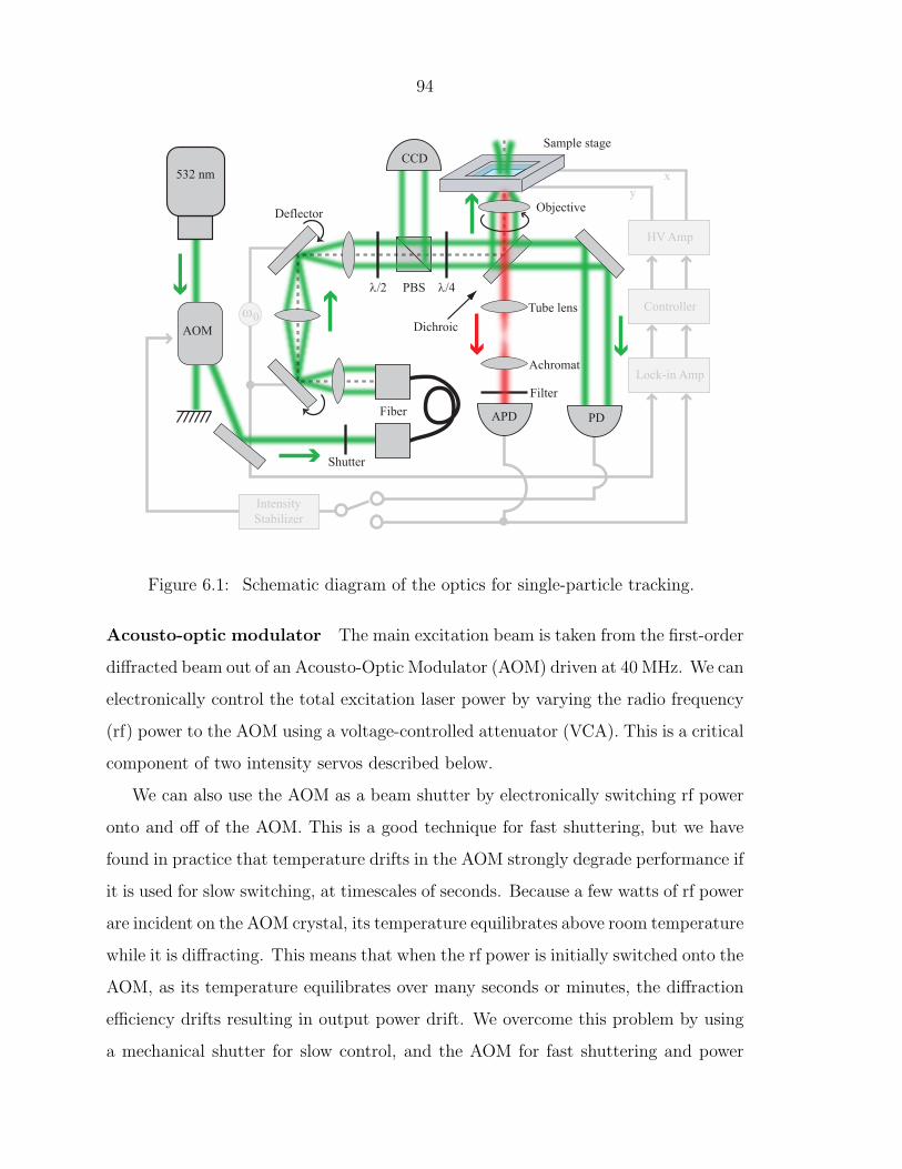
94

x

ω0

IntensityStabilizer

Controller

Lock-in Amp

HV Amp

y532 nm

AOM

Objective

APD

λ/2 λ/4PBS

Deflector

Sample stage

Fiber

DichroicTube lens

Achromat

Filter

Shutter

CCD

PD

Figure 6.1: Schematic diagram of the optics for single-particle tracking.

Acousto-optic modulator The main excitation beam is taken from the first-order

diffracted beam out of an Acousto-Optic Modulator (AOM) driven at 40 MHz. We can

electronically control the total excitation laser power by varying the radio frequency

(rf) power to the AOM using a voltage-controlled attenuator (VCA). This is a critical

component of two intensity servos described below.

We can also use the AOM as a beam shutter by electronically switching rf power

onto and off of the AOM. This is a good technique for fast shuttering, but we have

found in practice that temperature drifts in the AOM strongly degrade performance if

it is used for slow switching, at timescales of seconds. Because a few watts of rf power

are incident on the AOM crystal, its temperature equilibrates above room temperature

while it is diffracting. This means that when the rf power is initially switched onto the

AOM, as its temperature equilibrates over many seconds or minutes, the diffraction

efficiency drifts resulting in output power drift. We overcome this problem by using

a mechanical shutter for slow control, and the AOM for fast shuttering and power

95

modulation.

Mechanical shutter We use a clever mechanical shutter, brought from Germany

to the Mabuchi lab by Benjamin Lev. We use a small audio speaker, a tweeter, and

attach a flag onto its solenoid by cutting out the speaker fabric and gluing a stopper

into the speaker. Then by driving positive or negative current around the solenoid,

we pull the flag down or push the flag up into the laser. We have not optimized our

shutter, but it can easily block or unblock the laser in a few (1-10) ms, with excellent

extinction due to the mechanical beam blockage.

Optical fiber After the AOM and mechanical shutter, we run the beam through

a single-mode optical fiber (Thorlabs) both to achieve a nice Gaussian TEM00 beam

profile and to decouple the alignment of the AOM from the later optics. The fiber

introduces very large (and slow) drifts in output intensity and polarization, which we

think are cause by small pointing drifts at the fiber input. These drifts may arise

from air currents in the room, temperature drifts affecting the AOM, or just general

pointing instability in the laser itself. Because these are quite large amplitude, we

use an intensity servo (discussed below) to lock either the laser intensity itself or

to lock the fluorescence photon count rate during particle tracking. Because of the

polarization noise, one must take care to sense the correct polarization for the intensity

servo, because locking one of the polarization’s intensities increases noise in the other.

Beam deflection For particle tracking, we require a circularly rotating beam,

which we create using two resonant beam deflectors (Electro-Optic Parts Corporation,

EOPC) driven at 8 kHz. The deflectors are just small mirrors mounted on torsion

pendulums and driven sinusoidally (electromagnetically) with a phase difference of

90 provided by a phase-locked driver. In retrospect, 8 kHz was not a great choice for

the rotation frequency because it is at the upper end of the audible frequency spec-

trum, so the experiment makes a somewhat excruciating high-pitched whine while

operating. I would strongly suggest either acousto-optic modulation (with no moving

96

parts to radiate acoustically) or modulation at a frequency that is safely outside of

your audible range.

It was convenient to mount these deflectors so that they both deflect in the hor-

izontal direction, but of course for circular rotation of the beam, we need to convert

one horizontal deflection into a vertical deflection. To accomplish this, we used a

four-mirror arrangement that imparts a geometric phase and can in principle rotate

the beam shape (including polarization) by any angle. I thought this was a pretty

clever design, and it turns out it has been discussed in the literature in Refs. [44, 45].

It is quite a useful device though, so I suggest checking those references out.

Lenses should be arranged in such a way that they match the divergence angle

of the beam deflection patter with the divergence of the beam waist. Actually, by

slightly misaligning the beam waist divergence and the angular deflection, we can

achieve the desired situation in which the beam is focused to its minimum waist

but still rotates in a circular pattern at the focal plane of the microscope inside the

sample.

Filter optics Following the beam deflectors, the rotating beam is sent through a

standard half-waveplate, polarizing beamsplitter, quarter waveplate (λ/2-PBS-λ/4)

anti-retroreflection combination. This serves the dual purpose of circularly polariz-

ing the excitation beam and separating the retroreflected light from the sample for

imaging onto a CCD camera (discussed below). Since we focus light to a very sharp

focus, it is good to use circularly polarized excitation light so that interference effects

at glass interfaces cannot (by symmetry) result in any radially asymmetric intensity

profiles. During tracking, we are sensitive to radial asymmetries in the excitation

intensity, which turn up as offsets on the lock-in quadrature outputs, and these may

arise when focusing linearly polarized light through an interface at high numerical

aperture (N.A.) [46–49].

Dichroic filter 532 nm excitation light is reflected off of a 550 nm cutoff dichroic

long-wave pass beamsplitter. We have used a few different brands of optical filter

97

here and ultimately found superior performance with Chroma filters in virtually every

situation. In practice, because 532 nm is very close to the 550 nm cutoff wavelength, a

significant fraction of laser light is transmitted through the filter. We take advantage

of this imperfection, and focus this light onto a photodiode (PD) as a laser intensity

monitor.

Microscope objective We have used two infinity-corrected microscope objectives

in different situations: a Zeiss 100x/N.A. 1.4 plan-apochromat oil immersion objec-

tive and a Zeiss 63x/N.A. 1.2 c-apochromat water immersion objective. The former

objective was used for our earliest tracking results [25]. It has the advantage of very

tight beam focusing and is much lighter than the water immersion objective, but as

an oil immersion objective, it introduces substantial beam aberrations when focused

more than a few microns into an aqueous sample. The water immersion objective

provides slightly less tight focusing but much cleaner beam shapes and higher quality

tracking error signals. This objective was used for the studies of Refs. [27, 28].

CCD Camera We use an off-the-shelf CCD camera to image the retroreflected

532 nm laser intensity, which is separated from the incident light by the λ/2-PBS-

λ/4 unit. The incident and retroreflected beams interfere and give far-field diffraction

patterns at the CCD camera that are sensitive to the z position of the glass cover

slides that hold the sample at sub-wavelength distance scales [50]. These diffraction

patterns give a very useful visual queue to aid in focusing the apparatus.

Fluorescence collection Fluorescence is collected by the microscope objective and

transmitted through the dichroic filter. A Zeiss tube lens (f = +160 mm) then

refocuses the light. The microscope can be operated confocally by placing a pinhole,

typically 100 µm in diameter, at the tube lens focus. Fluorescence light is then

recollected by an achromatic doublet lens, and finally refocused by a second achromat

onto the single-photon counters (only one of these doublets is shown in Fig. 6.1).

98

Single-photon counters Fluorescence light is detected by a single-photon count-

ing avalanche photodiode operated in Geiger mode (Perkin-Elmer SPCM-14-AQR).

Each incident photon generates a 25 ns TTL pulse that is electronically split into four

signal paths at a digital fanout. The photon count rate is recorded at a computer,

sent to the lock-in amplifier for the tracking servo, low-pass filtered and displayed

on an oscilloscope for real-time monitoring, and finally the photon count rate can be

used as an error signal for feedback to the AOM controlling the intensity of the exci-

tation laser (see below). The computer and oscilloscope signal paths are not shown

in Figs. 6.1 and 6.3.

6.1.2 Sample volume

A schematic diagram of the sample volume for single-particle tracking experiments is

shown in Fig. 6.2.

Sample preparation For tracking, our samples are aqueous solutions of fluorescent

particles between glass microscope cover slides. We typically put between 1 and 10 µL

of liquid between glass microscope cover slips (22×40 mm, nominal thickness of 160

µm). The solution typically fills or almost fills the space between the slides, resulting

in a liquid layer around 1-2 µm deep. The sample depth can be determined by using

a confocal pinhole to limit detection efficiency in the z direction and subsequently

scanning a sample with high fluorophore concentration through the focus.

Our particles are fluorescently embedded polystyrene microspheres from Bangs

Laboratories. We use the dyes “Envy Green” and “Suncoast Yellow” and have beads

at diameters of 60 nm and 210 nm. Adding about 0.1% Tween-20 to deionized water

helps reduce aggregation in the beads. On the other hand, adding salt to the aqueous

solution strongly enhances aggregation and surface adhesion. Bangs Laboratories

has a very helpful website, http://www.bangslabs.com and a useful tech note about

aggregation in particular at http://www.bangslabs.com/technotes/202.pdf.

Also, preparation of the slides strongly affects adhesion of microspheres. We

have found that slides soaked for 30-60 min in 1M KOH are sufficiently clean that

http://www.bangslabs.com

http://www.bangslabs.com/technotes/202.pdf

99

532 nm

AOM

Objective

APD

λ/2 λ/4PBS

Deflector

Sample stage

Fiber

DichroicTube lens

Achromat

Filter

Shutter

CCD

PD

x

ω0

IntensityStabilizer

Controller

Lock-in Amp

HV Amp

y

Figure 6.2: Schematic diagram of the sample volume for single-particle tracking. Flu-orescent particles in aqueous solution diffuse freely in the xy plane, but are confinedby glass coverslips in the z direction. A tracked particle diffuses freely (in the axiallyconfined geometry) in the reference frame of the bulk fluid while the feedback controltranslates the entire sample volume in order to hold the particle on the laser axisdefined by x = y = 0. Because the sense of the laser rotation, and therefore the signof the feedback controller, reverses upon crossing the focal plane of the microscopeoptics, the sample mount is adjusted in the z direction so that the focal plane liesjust outside of the sample volume.

liquids spread nicely and adhesion is low. When we clean slides with more aggressive

procedures, the rate of surface adhesion actually increases.

The diffusion coefficient of a sphere of diameter d in a solution of viscosity η is

given by the Stokes-Einstein relation [51]

D =kBT

3πηd(6.1)

where kB is Boltzmann’s constant and T is the temperature. For water, η ≈ 10−3

Pa·s, so we find D = 2.1 µm2/s is the predicted value for the 210 nm diameter beads

100

and D = 7.2 µm2/s is the predicted value for the 60 nm beads. In some of our

very thin samples, we find reduced diffusion coefficients, which probably arise due

to particle reflections at the sample boundaries [52] and hydrodynamic “wall-drag”

effects [53, 54].

Piezo-electric stages Samples are mounted on a two-dimensional 100×100 µm

piezoelectric translation stage from Polytec, PI. The stage is driven by a high-voltage

amplifier module, from the same manufacturer, that also contains high-resolution

capacitive position sensors so that we can accurately monitor the x and y position of

the sample stage during tracking.

Sample mount The sample mount has evolved through many stages since our early

DNA experiments. The final incarnation was machined by Kevin McHale to mate

with the piezoelectric translation stage, and gave us easy, repeatable sample switching

capability. A key feature of this sample mount is its relative flatness, since earlier

sample mounts suffered from some degree of tilt that altered the relative separation

between the sample layer and the microscope objective as the sample translated in x

and y. To give an idea of the tolerance required, we routinely translate the sample

stage over its entire range of 100 µm, and a change in z of 1 µm over this range can

drastically alter the tracking parameters. Thus the stage must be level to better than

1 part in 100. This coupling between x, y, and z positions gave us some trouble until

Kevin’s newly machined stage eliminated most of the tilt.

6.1.3 Electronics

The electronics for single-particle tracking consist primarily of servos for stabilizing

the laser intensity, signal-processing electronics, tracking controllers, and high-voltage

amplifiers for driving piezoelectric stage positioners. These are described below, and

some of them are displayed in Fig. 6.3.

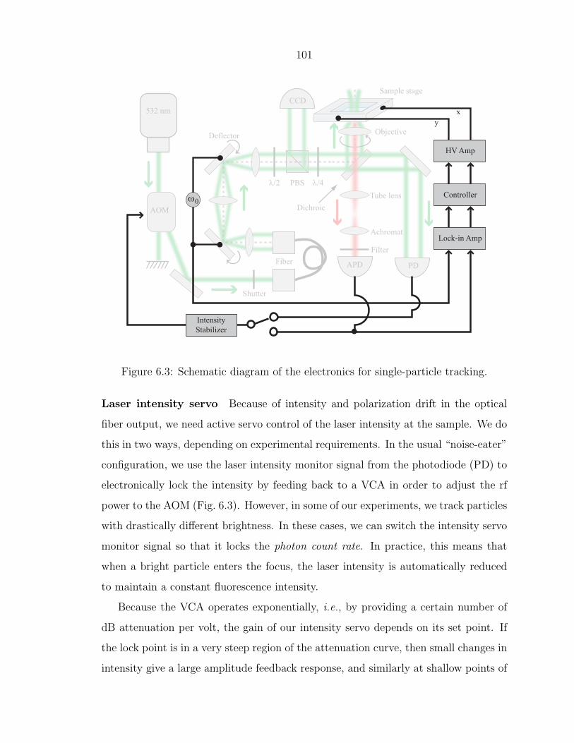
101

532 nm

AOM

Objective

APD

λ/2 λ/4PBS

Deflector

Sample stage

Fiber

DichroicTube lens

Achromat

Filter

Shutter

CCD

PD

x

ω0

IntensityStabilizer

Controller

Lock-in Amp

HV Amp

y

Figure 6.3: Schematic diagram of the electronics for single-particle tracking.

Laser intensity servo Because of intensity and polarization drift in the optical

fiber output, we need active servo control of the laser intensity at the sample. We do

this in two ways, depending on experimental requirements. In the usual “noise-eater”

configuration, we use the laser intensity monitor signal from the photodiode (PD) to

electronically lock the intensity by feeding back to a VCA in order to adjust the rf

power to the AOM (Fig. 6.3). However, in some of our experiments, we track particles

with drastically different brightness. In these cases, we can switch the intensity servo

monitor signal so that it locks the photon count rate. In practice, this means that

when a bright particle enters the focus, the laser intensity is automatically reduced

to maintain a constant fluorescence intensity.

Because the VCA operates exponentially, i.e., by providing a certain number of

dB attenuation per volt, the gain of our intensity servo depends on its set point. If

the lock point is in a very steep region of the attenuation curve, then small changes in

intensity give a large amplitude feedback response, and similarly at shallow points of

102

the attenuation curve the servo is comparatively slow. We can therefore use neutral

density filters to adjust the laser power at its source, so that at a given lock point, the

intensity servo sits at different points of the attenuation curve and exhibits different

gain and bandwidth. This is a convenient way to adjust the bandwidth of our in-

tensity servos, which becomes a critical parameter for the fluorescence intensity lock.

Although the VCA is quite fast, and we do not worry about driving it into instability,

we have to keep the servo bandwidth low for locking the photon count rate or else we

will feed photon counting shot noise into the system.

Lock-in amplifier We use a dual-phase digital lock-in amplifier (Stanford Research

Systems, SRS850). The photon counter output is buffered by a digital fanout circuit

and then fed directly onto the voltage sensing input of the lock-in. The reference

is taken from the beam deflector drive signal. We typically use gain settings in the

range 28–54 dB, filter time constants of 300 µs to 1 ms, and rolloff rates of 12 or 18

dB/oct.

Tracking controllers For tracking, we initially used a programable digital mi-

crocontroller (Analog Devices, ADuC7024). Analog Devices supplied us with a test

board and software (Keil µVision) that allowed us to program the microcontroller

in C and download instructions onto the chip via USB interface. I wrote MATLAB

software to convert arbitrary transfer functions into discrete time filters and load the

coefficients onto the board. An example of one of the LQG control laws of Ch. 2 im-

plemented using the microcontroller is shown in Fig. 6.4. It successfully implemented

“arbitrary” transfer functions in this way, but with disappointingly low bandwidth

and noise due to sampling and timing errors. Once loaded with even a second-order

filter, the effective bandwidth of the microcontroller was barely 1 kHz. For higher-

order filters, timing errors (missed samples and updates) accumulate and bandwidth

continues to fall. Our original hope had been to implement the LQG filters designed

in Ch. 2, but these were simply too high order to implement at sufficient bandwidth.

For our first successful tracking experiments [25], we used a proportional-integral

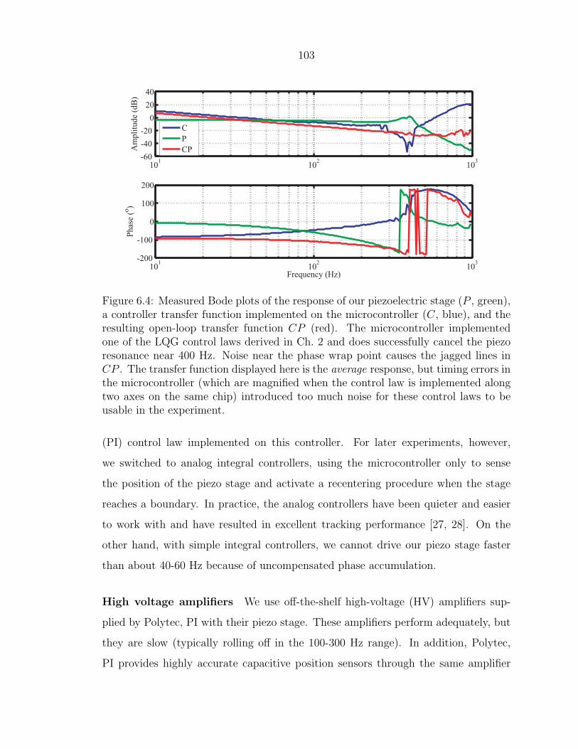
103

101

102

103

-60

-40

-20

0

20

40

Am

pli

tude

(dB

)

101

102

103

-200

-100

0

100

200

Frequency (Hz)

Phas

e (o

)C

P

CP

Figure 6.4: Measured Bode plots of the response of our piezoelectric stage (P , green),a controller transfer function implemented on the microcontroller (C, blue), and theresulting open-loop transfer function CP (red). The microcontroller implementedone of the LQG control laws derived in Ch. 2 and does successfully cancel the piezoresonance near 400 Hz. Noise near the phase wrap point causes the jagged lines inCP . The transfer function displayed here is the average response, but timing errors inthe microcontroller (which are magnified when the control law is implemented alongtwo axes on the same chip) introduced too much noise for these control laws to beusable in the experiment.

(PI) control law implemented on this controller. For later experiments, however,

we switched to analog integral controllers, using the microcontroller only to sense

the position of the piezo stage and activate a recentering procedure when the stage

reaches a boundary. In practice, the analog controllers have been quieter and easier

to work with and have resulted in excellent tracking performance [27, 28]. On the

other hand, with simple integral controllers, we cannot drive our piezo stage faster

than about 40-60 Hz because of uncompensated phase accumulation.

High voltage amplifiers We use off-the-shelf high-voltage (HV) amplifiers sup-

plied by Polytec, PI with their piezo stage. These amplifiers perform adequately, but

they are slow (typically rolling off in the 100-300 Hz range). In addition, Polytec,

PI provides highly accurate capacitive position sensors through the same amplifier

104

module, but these too have slow rolloffs at the same bandwidths. So although the

amplifiers are nicely packaged and integrated, the experiment could benefit from an

upgrade to faster electronics. However, all of the experimental results reported here

used these amplifiers. On another note, on three separate occasions, we bought Poly-

tec piezo stages with unstable position servo loops. (even unloaded and right out of

the box). In all these cases, we simply locked these using Polytec’s position sensors

and HV amps and a home-built controller circuit.

Dynamic signal analyzer We measure transfer functions using the swept sine

response function of an SR785 dynamic signal analyzer (Stanford Research Systems).

This instrument can measure response curves all the way down to DC.

6.1.4 Data acquisition and computer software

Time-interval analyzer We use the GT653 time-interval analyzer (TIA) from

Guide Technologies installed on the PCI slot of a Micron PC to record fluorescence

photon arrival times. This board has high time resolution (0.5 ns) and is capable of

recording >106 photon arrival times in a single shot before filling the onboard memory.

Kevin McHale has also written software to read samples continuously from the board,

so that as long as the read rate to the computer is faster than the photon arrival rate

the sample memory is limited by the computer hard drive. These boards are nice

and easy to program, but they suffer from the major drawback that they have only

two channels and synchronization between separate boards does not work (although

software calls and documentation for this function exist). This is not an issue for

the experimental results presented here, but our experiment is actually capable of

recording data on two TIA boards and four photon counters simultaneously, but

these still cannot be synchronized in the data acquisition despite repeated inquiries

with technical support.

National Instruments DAQ card In addition to the TIAs for recording photon

arrivals, we use a National Instruments data acquisition card (NI-DAQ), the PCI-

105

MIO-16E-4, installed on a Dell PC. This card provides analog and digital inputs and

outputs as well as timing capability so it really is a workhorse of the experiment. All

of the software to drive it was written in C (we do not use LabView). In a typical

experimental run, the x and y position of the piezoelectric stage and the monitor

photodiode signal are all digitized and recorded with the NI-DAQ card. Furthermore,

beam shutters (both through the AOM and mechanical shutter) and APD gates are

computer-controlled using the digital outputs from the same card and (when not

tracking) the x and y position of the piezoelectric stage can be set using the analog

outputs from the NI-DAQ card.

Interfacing the computers The TIAs and NI-DAQ cards are on separate com-

puters to alleviate the large computational, memory, and scheduling demands of

running these cards simultaneously on a single computer. Furthremore, the broad

functionality of the NI-DAQ card, and my own creative C coding, has led to some

extremely violent system crashes, and it seemed wise to physically isolate the delicate

and expensive TIA cards from the specter of physical memory dumps and paging file

errors. In a typical experiment, we wish to make software alternating software calls

at different cards, for example:

1. Step sample stage (NI-DAQ analog output).

2. Ungate APD (NI-DAQ digital output).

3. Begin photon counting (TIA).

4. Unblock laser (NI-DAQ digital output).

5. Begin record laser intensity (NI-DAQ analog input).

6. Wait for memory to fill (TIA).

7. Gate APD (NI-DAQ digital output).

8. Block laser (NI-DAQ digital output).

106

In order to make these types of software calls, I defined a master (Micron) and

a slave (Dell) computer and used Windows sockets to pass messages such as those

above back and forth between the separate computers, via ethernet. With these

socket protocols, and MATLAB wrappers for all the C executables, we can execute

sequence such as the one shown above entirely in a MATLAB script on the master

computer. This has turned out to be extremely useful in practice. A great socket

programming guide is online: http://beej.us/guide/bgnet/.

Correlation software A note about calculating correlation functions is warranted

here. Because our TIAs record individual photon arrival times, we have the capability

to measure FCS curves g(τ) over many orders of magnitude in τ by post-analyzing

the data. However, calculation of g(τ) using standard methods based on the Wiener-

Khinchin theorem and the fast-Fourier transform (FFT), for example xcorr.m in

MATLAB, has two primary drawbacks. First, statistical bias at large lag times (com-

pared to the length of the entire data sequence) arises from the redundant weighting

of noise. This problem is easily circumvented using a symmetric normalization:

g(τ) =1

T−τ

∫ T−τ

0δI(t)δI(t+ τ)dt(

1T−τ

∫ T−τ

0I(t)dt

)(1

T−τ

∫ T

τI(t)dt

) . (6.2)

The second more troublesome issue is that the correlation function found using an

FFT must be calculated over linearly spaced time intervals τ , giving a potentially

huge autocorrelation vector. For example, if we use a time bin ∆τ = 0.1 µs and

calculate the correlation function out to 1 s, the resulting vector contains 107 data

points. Well-known methods such as the “multiple-tau” algorithm get around this

problem by calculating correlation functions at logarithmically spaced time intervals

[55]. However, these algorithms still do not satisfy all of our demands, because they

average the correlation function over logarithmically increasing intervals. For a peri-

odic signal (such as the one obtained with our rotating laser), we may wish to see the

fast periodic structure at large time scales. A nice solution to these problems comes

from an algorithm described in Ref. [56], which allows us to calculate correlation

http://beej.us/guide/bgnet/

107

0 5 10 15 200

5

10

15

x 104

Co

un

ts [

s-1]

t [s]

Figure 6.5: Typical open-loop transit of a 60 nm microsphere through the excitationvolume. The excitation laser was not rotating for this measurement.

functions at arbitrary time lags and over arbitrary bin sizes directly from photon

arrival time data. Using this algorithm, we can easily form a correlation function on,

say, 1000 time intervals of size ∆τ = 0.1 µs evenly distributed between τ = 0.1 µs and

τ = 1 s. We coded a version of this algorithm in C and compiled it into a MATLAB

.m executable using MEX methods.

6.2 Calibration and diagnostics

In this section, some typical experimental measurements are discussed and exam-

ples are given. These include diagnostic and calibration measurements, as well as

interesting observations about the behavior of the tracking system.

6.2.1 Open-loop measurements

For a typical open-loop measurement, we load the sample with 2 µL of 60 nm “Envy

green”-labeled microspheres between glass coverslips, as described above. As these

108

0 5 10 15 200

5

10

x 104

t [s]

Counts

[s-

1]

Figure 6.6: Typical open-loop transit of a 60 nm microsphere through the excitationvolume with the excitation laser rotating at 8 kHz.

particles diffuse into and out of the laser focus, we collect typical fluorescence transits

of the type shown in Fig. 6.5. For that measurement, the excitation beam was static

(i.e., not rotating, as in the tracking configuration). A second measurement on the

same sample recorded with the rotating excitation laser is shown in Fig. 6.6

To make a quantitative comparison between transits recorded with and with-

out the beam rotation, we performed fluorescence correlation spectroscopy (FCS) on

each of these samples. The fluorescence correlation function g(τ) was calculated as

described in Sect. 6.1.4. For a two-dimensional sample, denote by g0(τ) the predicted

correlation function for particles with diffusion coefficient D diffusing in a Gaussian

laser with beam waist w:

g0(τ) =1

N

(1 +

τ

τD

)−1

, τD =w2

4D. (6.3)

If we then rotate the excitation laser at frequency ω0 along a circle of radius r about

109

10-6

10 -5

10 -4

10 -3

10 -2

10 -1

100

101

102 -0.5

0

0.5

1

1.5

2

τ [s]

g(τ

)

Figure 6.7: Open-loop FCS curve (solid blue line) together with a fit to g0(τ) definedby Eq. (6.3) (dashed red line). The fit parameters were N = 0.53 and τD = 0.335s.

its axis of propagation, the correlation function becomes

gr(τ) = g0(τ) exp

[−2

r2

w2

(1− cosω0τ

1 + τ/τD

)]. (6.4)

These are standard calculations that can be derived from the expressions in Sect.

5.2.2.

The correlation functions in Figs. 6.7-6.8 were calculated from photon arrival-

time data, and from curve fitting we find a diffusion time τD = 0.33− 0.34s. In order

to convert these diffusion time estimates into diffusion coefficients, we require the

beam waist w. Later, when we track these particles, we will be able to measure the

diffusion coefficient directly from their translational motion. However, we performed a

calibration that is typical of open-loop methods: we found a bead adhered to the glass

coverslip surface and raster scanned it in order to map the beam profile. The resulting

profiles are shown in Fig. 6.9 for both the stationary laser and for the rotating laser.

A Gaussian fit to the beam profile data reveals a slightly asymmetric beam profile

110

10-6

10 -5

10 -4

10 -3

10 -2

10 -1

100

101

102

-0.5

0

0.5

1

1.5

2

2.5

τ [s]

g(τ)

Figure 6.8: Open-loop FCS curve (solid blue line) with the laser rotating, togetherwith a fit to Eq. 6.4 (dashed red line). The fit parameters were N = 0.41, τD = 0.330s,r/w = 0.21.

with waist wx = 3.2µm in the x direction and wy = 2.9µm in the y direction. Curve

fitting of the autocorrelation function in Fig. 6.7 did not detect any asymmetry. [The

theoretical form of g(τ) for the asymmetric case is easily found from Eq. (5.59).] The

fit also reveals that our laser has fatter tails than a Gaussian. Such deviations from a

Gaussian profile can have a profound effect on particle transport properties inferred

from open-loop FCS, and it becomes a major advantage of closed-loop methods that

we can completely suppress such complications. Incidentally, a fit to a scan of the

same same stuck bead, but with the rotating laser, gives a rotation radius of r = 1.0µm

or r/w = 0.33. Note that in later tracking results from Chs. 7 and 8, we will use a

smaller beam with w = 1.0 µm and r = 0.6 µm.

Taking the mean of wx and wy to find w = 3.05 µm, we estimate a diffusion

coefficient D = 6.9 µm2/s for these particles. This is in good agreement with the

Stokes-Einstein value, but note that a ±5% variation in the beam waist leads to

a diffusion coefficient ranging between 6.2 and 7.5 µm2/s, a 21% variation. This

111

3436

3840

42

8486

8890

920

2

4

6

8x 10

4

x [µm]y [µm]

Cou

nts

[s−1 ]

Figure 6.9: Measured Gaussian laser intensity profile. The sample stage was rasterscanned across a single immobilized 60 nm diameter bead while the fluorescenceintensity was recorded. A fit to this data reveals a slightly asymmetric profile withbest-fit Gaussian beam waists of wx = 3.2µm in the x direction and wy = 2.9µm in they direction. The laser has fatter tails than a true Gaussian distribution. The spike influorescence near (x, y) = (41, 88) µm appeared when a freely diffusing particle passedthrough the sample (this data point was omitted in the curve fitting procedure).

3436

3840

42

8486

8890

920

2

4

6

8x 10

4

x [µm]y [µm]

Cou

nts

[s−1 ]

Figure 6.10: Example of the laser intensity profile for the rotating beam, measuredin the same way and on the same particle as the data in Fig. 6.9. Using w measuredfor the stationary beam, we find a rotation radius r = 1.05 µm giving a beam shapeparameter r/w = 0.33. Note that the time average of a rotating beam will not assumea “crater” shape on the rotation axis until r/w & 0.6.

112

−4 −2 0 2 4−0.1

−0.05

0

0.05

0.1

x [µm]

Lock

−in

Out

put [

V]

Figure 6.11: Measured error signal for closed-loop tracking. The measurement wasmade by scanning the piezo stage past a bead that had stuck to the surface either byelectrostatic adhesion or pinning between the coverslips. The dotted line is a fit toEq. (3.35) with x = ρ cos θ.

steep dependence of the diffusion coefficient estimate (an intrinsic property of the

particle in its environment) on the beam shape (an experimental artifact) is a major

disadvantage of FCS. Again, our closed-loop control techniques allow much more

accurate measurements of the diffusion coefficient with very little dependence on

beam shape parameters. Furthermore, the parameters measured here are averaged

over an ensemble of transits from many different particles, whereas the values we will

measure during closed-loop tracking result from truly single-particle interrogations.

6.2.2 Measuring the error signal

For very thin liquid samples, our microspheres occasionally become immobilized on

the glass coverslip surfaces by electrostatic adhesion or by pinning between the cover

slides as the liquid evaporates from the slide. For long tracking runs (>1 hour), such

degradation eventually compromises the sample. However, an immobilized fluorescent

particle is a very useful diagnostic tool, and we can study our error signal with it.

An example of such a measurement is shown in Fig. 6.11, in which the piezo stage

was scanned in the x direction over an immobilized bead and the cosine quadrature

of the lock-in output was recorded. The plot does not give all the information about

113

the scan, because the scanning time is not displayed. However, this error signal was

recorded with only a few ms spent over the high-intensity region of the laser, i.e., the

linear region of the error signal.

Plotting both the x and y error signals (the cosine and sine quadratures of the

lock-in output) against each other on an oscilloscope leads to plots like those shown

in Fig. 3.3. Two important features of the error signal can be observed and adjusted

using an immobilized bead: the sign of the error signal and its symmetry with respect

to positive and negative deviations. For a one-dimensional servo, you can usually get

away with an inverter switch for finding the correct sign of the control law from the

two possibilities. For our two-dimensional tracking problem, there are four possible

combinations of signs for the x and y error signals, and a systematic method for

finding signs is a little more important than in the one-dimensional case. Second,

the symmetry of the error signal can be degraded especially by imperfections in

the photon counting collection optics. The APD active area is only 170 µm, and

imperfect focusing of fluorescent light onto the detector leads to asymmetric error

signals and impaired tracking capability. We use achromatic doublet lenses in the

fluorescence beam path for good, wide spectrum focusing. While maximizing the

observed fluorescent intensity from a bright sample can be a useful alignment method,

symmetrization of the error signal turns out to be more directly helpful.

115

Chapter 7

Closed-Loop Particle Tracking

In this chapter, we finally achieve full closed-loop fluorescent particle tracking. First,

we present lock results for an immobilized bead, then take a “historical” perspective,

discussing some of our early tracking successes and moving on to more recent and

much improved tracking data.

7.1 Closing the loop

Using the same type of immobilized bead discussed in Ch. 6, we can finally attempt

to lock a particle’s position by feeding the measured position error signal back to

the piezoelectric sample stage. Once the error signals are symmetrized and scaled

to have the correct signs and magnitudes, we can use analog integrators or digital

microcontrollers to lock an immobilized bead to the optic axis of the microscope.

In this configuration, we can measure the transfer function response of the tracking

system by adding a sinusoidal driving signal onto the error signal and letting the

feedback network compensate for the disturbance by maintaining the locked particle’s

position. The transfer function from this added signal to the piezo stage position is

TEX = 1/(1+CP ) using the controller and plant notation from chapter 5. An example

of such a swept sign response is shown in Fig. 7.1 and the expected qualitative shape

of such a transfer function is shown in Fig. 7.2. The strong suppression of the

disturbance at low frequencies frequencies is an unambiguous indication of a locked

particle.

116

SRS

36.11005 Hz -137.7 deg

10 Hz

Freq. Resp. Phase• 144 s

300 Hz-250

deg

250

deg

50

deg/div

B Done

SRS

36.11005 Hz 6.213 dB

10 Hz

Freq. Resp. Log Mag 144 s

300 Hz-8

dB

12

dB

2

dB/div

A Done

6/09/06 17:26:57

Figure 7.1: Bode plot of the measured transfer function of the closed-loop trackingsystem locked to an immobilized fluorescent microsphere. A swept sine was added tothe error signal and the dynamic response of the sample stage was measured. At lowfrequencies, the disturbance is strongly attenuated. Nonlinear behavior (arising fromthe Gaussian, not parabolic, shape of the laser profile) sets in near 200 Hz.

7.2 Early experimental success

The data presented in this section was recorded in March 2005 and published in Ref.

[25]. For these measurements, we used 1-2 µL 0.1 nM concentration fluorescent micro-

spheres (60 nm diameter). The excitation laser power was ∼1–10µW for exciting the

fluorescently labeled beads, giving overall photon count rates of ∼105/s, comparable

to the count rates of bright individual dye molecules excited by a correspondingly

higher laser power.

117

20

10

0

10

Mag

nit

ud

e (d

B)

100

101

102

103

180

135

90

Ph

ase

(deg

)

Frequency (Hz)

Figure 7.2: Bode plot of a closed loop transfer function TXE = 1/(1 + CP ) whenCP is a simple integrator. Note the qualitative similarity between the low-frequencybehavior of this transfer function and the measured one in Fig. 7.1 both in magnitudeand phase.

7.2.1 Tracking data

A successful tracking trajectory is shown in Fig. 7.3. From the data in the figure, we

see that the tracking controller maintains a relatively constant fluorescence intensity

for about 2.5 s, while the stage position moves well over 10 µm along both the x

and y axes. The residual fluctuations arise from the feedback control bandwidth,

as discussed theoretically in Ch. 5, but also from the uncontrolled motion of the

particle in the axial (z) direction. As a comparison, note that the only other closed-

loop tracking results in the literature at the time of these measurements were those

presented in Ref. [16]. In that study, 500 nm diameter beads in an agarose gel

were tracked in three dimensions with impressively high spatial accuracy but at very

slow timescales relative to our work. The particle trajectory shown in that study

remained within a cube 3 µm on a side for 100 s, whereas our data shows a single

particle tracked at one point across ∼5 µm in about less 0.5 s, two to three orders of

118

7 7.5 8 8.5 9 9.5 100

200

400

600

800

7 7.5 8 8.5 9 9.5 1010

15

20

t (s)

Po

sitio

n (

µm

)C

ou

nts

/2 m

s

Figure 7.3: Tracking data from one of our earliest successful runs. The upper plotshows fluorescence data, and the lower plot shows the x (solid) and y (dotted) posi-tions of the sample stage during the fluorescence trace. Just before 7.5 s, a particlediffused into the capture region and the controller responded by moving the samplestage to track this particle. The irregular motion of the sample stage at 7.6 s re-sulted from an (expected) arithmetic overflow in the microcontroller. The residualfluorescence fluctuations during tracking arise from the competition between diffusionand feedback control and also from the uncontrolled motion of the particle in the zdirection.

magnitude faster than previously demonstrated.

7.2.2 Estimation of D

As a first interesting measurement based on our data, we can estimate the isotropic

diffusion coefficient D for this microsphere from the position of the sample stage

during tracking. While the particle is (approximately) locked on the laser axis by the

feedback controller, the xy position of the sample stage provides a bandwidth-limited

filtration of the particle’s position. Let the change in a particle’s x position during

a time interval ∆t be given by ∆X∆t, and similarly for y. Then we may construct a

simple estimator D for a particle’s diffusion coefficient D based on the mean-square-

deviation MSD(∆t) of the sample stage trajectory. As usual, let X(t) and Y (t) be

119

8 8.5 9 9.5 10

0

2

4

6

8

10

12

t (s)

0 0.05 0.1 0.15 0.21

2

3

4

5

6

7

8

9

∆t (s)

D (

µm

2/s

)^

Figure 7.4: Time-converging estimate of the diffusion coefficientD for the microspheretracking data in Fig. 7.3 with bin time ∆t = 20 ms. The dotted lines are 1σ errorestimates calculated for the estimator D, assuming underlying Brownian statistics.Inset: Final estimate of D as a function of bin time ∆t. For bin times larger than∼ 10 ms, the estimates are roughly constant with mean value D = 6.2 µm2/s.

the sample stage coordinates during tracking, and let ∆X∆t(t) = X(t+ ∆t)−X(t).

Then MSD(∆t) and D∆t are defined by

MSD(∆t) =1

2

σ2

∆t(X) + σ2∆t(Y )

(7.1)

D∆t =MSD(∆t)

4∆t(7.2)

where σ2∆t(X) denotes the variance of ∆X∆t over the sample trajectory (we will be

very precise about the calculation of this variance in Sect. 8.3). The result of this

estimate, formed as an accumulating average over the trajectory shown in Fig. 7.3

is shown in Fig. 7.4. The estimate of D converges to a value 6.2 µm2/s, close to the

value 7.2 µm2/s predicted by the Stokes-Einstein relation for 60 nm diameter beads in

water at room temperature. It is possible that surface adhesion slightly reduced the

120

effective diffusion coefficient. We do not suspect induced optical dipole forces to give

any significant trapping effect, since only a moderate trapping effect was observed for

1 mW of near-IR laser power on microspheres with 276 nm diameter in [18], whereas

we use smaller microspheres and only 1-10 µW of 532 nm light. A detailed analysis

of optical trapping effects in FCS experiments can be found in [57].

We can also vary ∆t, which should not change D∆t for pure Brownian motion.

However, when ∆t is smaller than the inverse closing bandwidth of the controller,

then the sample stage will exhibit reduced variations on this timescale, and we will

tend to underestimate the resulting diffusion coefficient with Eq. (7.2). It is easy to

see this by considering an extreme case: imagine binning the particle’s position over

extremely small intervals, much smaller than the response time of our piezoelectric

sample stage (say, 1 µs). Then in each time interval ∆t, the sample stage cannot track

the diffusing particle (although the particle does not move far enough to escape the

tracking controller) and only follows an “average” trajectory. The sample stage will

move a distance proportional to ∆t (i.e., at a fixed velocity along the averaged particle

trajectory) for these very small bin times, while the particle itself moves a distance

proportional to√

∆t (the characteristic property of Brownian motion). For small

enough ∆t, then, the estimator given by Eq. (7.2) will dramatically underestimate

the particle’s diffusion coefficient (by a factor proportional to√

∆t). As ∆t becomes

much larger than the inverse closing bandwidth, however, the sample stage can move

sufficiently fast to track the detailed motion of the particle within a single bin interval.

In this case, we expect a good statistical estimate of D from Eq. (7.2), but with a

concomitant increase in the estimator variance due to the smaller number of bin

intervals per fixed-length trajectory. Estimates constructed in this way are shown

in Fig. 7.4, along with error bars calculated for the estimator Eq. (7.2) assuming

underlying Brownian motion statistics (see Ch. 8 and Ref. [58] for details about

statistical estimation and error estimates). Of course, a quantitative version of these

arguments involves calculation of the statistics of the mean-square deviation in the

sample stage position; we already found this result in Ch. 5.

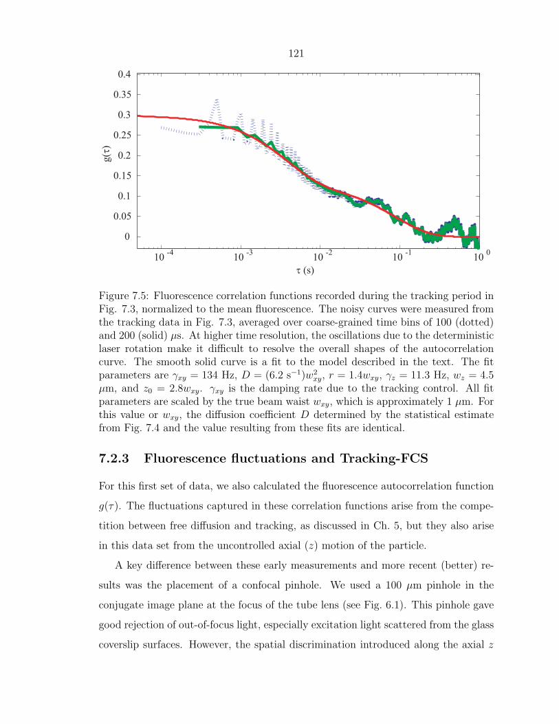
121

10-4

10-3

10-2

10-1

100

0

0.05

0.1

0.15

0.2

0.25

0.35

0.4

τ (s)

g(τ

)0.3

Figure 7.5: Fluorescence correlation functions recorded during the tracking period inFig. 7.3, normalized to the mean fluorescence. The noisy curves were measured fromthe tracking data in Fig. 7.3, averaged over coarse-grained time bins of 100 (dotted)and 200 (solid) µs. At higher time resolution, the oscillations due to the deterministiclaser rotation make it difficult to resolve the overall shapes of the autocorrelationcurve. The smooth solid curve is a fit to the model described in the text. The fitparameters are γxy = 134 Hz, D = (6.2 s−1)w2

xy, r = 1.4wxy, γz = 11.3 Hz, wz = 4.5µm, and z0 = 2.8wxy. γxy is the damping rate due to the tracking control. All fitparameters are scaled by the true beam waist wxy, which is approximately 1 µm. Forthis value or wxy, the diffusion coefficient D determined by the statistical estimatefrom Fig. 7.4 and the value resulting from these fits are identical.

7.2.3 Fluorescence fluctuations and Tracking-FCS

For this first set of data, we also calculated the fluorescence autocorrelation function

g(τ). The fluctuations captured in these correlation functions arise from the compe-

tition between free diffusion and tracking, as discussed in Ch. 5, but they also arise

in this data set from the uncontrolled axial (z) motion of the particle.

A key difference between these early measurements and more recent (better) re-

sults was the placement of a confocal pinhole. We used a 100 µm pinhole in the

conjugate image plane at the focus of the tube lens (see Fig. 6.1). This pinhole gave

good rejection of out-of-focus light, especially excitation light scattered from the glass

coverslip surfaces. However, the spatial discrimination introduced along the axial z

122

direction by the confocal pinhole leads to strong variation in the fluorescence inten-

sity as a particle “bounces” back and forth between the glass surfaces. This axial

discrimination led to enhanced fluorescence fluctuations, beyond those described by

the Ornstein-Uhlenbeck statistics of Ch. 5.

To give at least a qualitative model of this axial fluctation, we may assume the

glass surfaces to be reflecting boundaries for the relevant case of low surface adhesion.

Green’s functions for free particle motion and corresponding fluorescence autocorrela-

tion functions have been calculated as an infinite series for a Gaussian beam focused

symmetrically between two reflecting planes [7]; the resulting series have been ap-

proximated efficiently in [52], but I am unaware of an extension of these results to

reflecting planes in an asymmetric configuration. Instead of tackling this difficult

analytical problem, we instead approximate the reflecting boundaries in a way that

naturally fits the formalism developed here: we introduce a third Ornstein-Uhlenbeck

particle trap in the z dimension with corresponding damping rate γz and let the beam

profile in the z direction be characterized by an offset z0 and waist wz. This trap

is not due to the closed-loop particle tracking; it is nothing more than a tractable

approximation for a particle between two reflecting planes that are placed asymmet-

rically about the laser focus. The measured fluorescence correlation function and

the calculated model, with a symmetric beam Gaussian beam profile and first-order

damping at rate γxy along the x and y directions plus another first-order damping

rate γz along the axial direction, is shown in Fig. 7.5. The fit to this model contains a

lot of parameters, so it should be taken mostly as a forward correspondence between

reasonable parameters and the measured fluctuations, rather than as a method for

determining those parameters. In later, cleaner results we will see that the fits can

give truly quantitative results.

7.3 Tracking improvement

Following the first set of tracking results described in the previous section, a handful

of major experimental improvements were initiated. First, we removed the confocal

123

pinhole and eliminated virtually all axial (z) discrimination arising from the detection

optics. The detrimental effects of the confocal pinhole turned out to outweigh the

benefit of reduced background signal at our very low laser powers. This resulted

in a scenario much closer to the desired quasi-two-dimensional tracking scenario,

and served the dual purpose of reducing the axial-motion-induced fluctuations in

fluorescence during tracking and, more importantly, improving the tracking efficiency

by suppressing any dependence of the error signal on z. Second, we replaced the

digital microcontroller used for the first tracking results with analog integrators and

adjusted the gain between lock-in amp and controller circuits to maximize our signal-

to-noise ratio. The microcontroller was reassigned to the task of detecting when

the piezoelectric sample stage reached the edge of its travel region and subsequently

triggering an integrator reset procedure to recenter the apparatus, discarding any

currently tracked particle in the process. As an added technical benefit, the analog

integrators and their bipolar 15 V output swing, in contrast to the microcontroller’s

unipolar 2.5 V range, allowed us to track all the way to the limits of the piezoelectric

stage travel without additional, noise-inducing post-amplification.

These improvements led to tracking runs of the type shown in Fig 7.6. This run

was taken with a sample prepared essentially identically to the one used for the early

experiments. In Fig. 7.6, we monitor a 60 nm bead as it traverses ∼50 µm over 65

s, and fluorescence fluctuations are quite small relative to the earlier measurements.

Note that there was no servo controlling fluorescence fluctuations in this data (as

will be the case later), and the quieter nature of the fluorescence intensity is a direct

consequence of the tight tracking lock. The lack of a fluorescence servo is obvious

from the photobleaching decay of the fluorescence observed during the tracking period.

Although the beads are very bright and contain many dye molecules, after we have

collected tens of millions of photons in closed loop we still see some photodamage.

This data was taken in early 2006, and we recorded 74 trajectories of this type,

ranging in duration from a few seconds up to a maximum of 100 s, in the same data

set. As usual, during a tracking trajectory, we record time-sequences of positions

X = X(t) and Y = Y (t) of the sample stage during tracking. The estimate D∆t

124

20 30 40 50 60 70 80 90 1000

0.5

1

1.5

2x 10

5

20 30 40 50 60 70 80 90 10060

80

100

120

t [s]

Co

un

ts/s

Po

siti

on

[µ

m]

Figure 7.6: Typical tracking trajectory data. The upper plot shows the fluorescencecount rate in 10 ms time bins; the lower plot shows the x and y positions of the samplestage during the trajectory. The particle is lost when the sample stage reaches theend of its travel range. Note the 15% decay in fluorescence of the particle due tophotobleaching over the ∼65 s trajectory. The dotted line shows an exponential fitto the decay curve.

from the data in Fig. 7.6 with ∆t = 0.4s is shown in Fig. 7.7, as a running estimate

over the trajectory length. The error bars are at the 2σ level. With our large data

set, we can also look at statistics of the tracking events as an ensemble. For each

of the 74 two-dimensional trajectories in our data set, we may estimate the diffusion

coefficients D∆t(X) and D∆t(Y ) along separate Cartesian directions and over a range

of sample times ∆t. The (unweighted) average of the diffusion coefficient estimates

formed in this way are displayed in Figure 7.8 as ∆t is varied between 0.002 and 2 s.

At small time intervals, the D∆t contains contributions from the particle’s diffusion

as well as the feedback dynamics of the tracking apparatus. At longer times, the

variance is dominated by the particle’s motion and depends only on the particle’s

diffusion coefficient.

125

30 40 50 60 70 800

2

4

6

8

10

12

14

16

t [s]

D∆

t

Figure 7.7: Running diffusion coefficient estimates D∆t(X) and D∆t(Y ) from thedata shown in Fig. 7.6, for ∆t = 0.4 s. The error bars are at the 2σ level, assumingunderlying Brownian motion statistics.

Correlation functions with exponential fluorescence decay The appearance

of exponential photobleaching decay in our fluorescence signals gives a contribution

to the fluorescence correlation function that can be easily accounted for. Suppose

that a fluctuating signal I0(t) is also subject to exponential decay so that we may

write the total signal I(t) = e−γdtI0(t). We can calculate the autocorrelation function

of I(t) assuming that the decay timescale γd is much longer than the other timescales

in the signal I0(t). Let T be the total measurement time. Plugging in to Eq. 6.2, we

easily find

g(τ) =

[γ(T − τ)

2

]coth

[γ(T − τ)

2

][g0(τ)− 1] + 1 (7.3)

where coth is the hyperbolic cotangent function and g0(τ) is the fluorescence au-

tocorrelation function in the absence of photobleaching fluorescence decay, i.e., the

autocorrelation of I0(t).

Distribution of exit times from a square region One interesting statistical

effect arising in the analysis of extremely long tracking runs should at least be men-

tioned here. At extremely long bin times (and with enough data), we expect D∆t to

126

0 0.5 1 1.5 25

6

7

8

9

10

11

12

∆ t

D∆

t

Figure 7.8: Diffusion coefficient estimates D∆t(X) and D∆t(X) averaged over the 74trajectories in our data set and plotted as a function of the sample time ∆t.

decrease with ∆t because we post-select trajectories which remain within the travel

range of our tracking apparatus, approximately L = 100µm in each direction. In

other words, at extremely long bin times, only trajectories that remained within the

trackable region for an anomalously long time contain enough data to form an esti-

mate D∆t. We will not attempt a systematic analysis of this effect, but note that its

contribution is expected to arise for trajectories whose length approaches the length-

scale TL = L2/π2D ≈ 156 s.

To see where TL arises, we should derive the exit-time distribution for a particle in

a square region of width L. To do this, we calculate the solution to the free-diffusion

Fokker-Planck equation with absorbing boundary conditions, so that the integrated

probability over this region is equal to the probability that a particle has not exited

the region [36, 31]. It is easy to see that, for a particle restricted to the region

L = [0, L]× [0, L], with absorbing boundary conditions at the edges of the square, the

127

10−6

10−5

10−4

10−3

10−2

10−1

100

101

1

1.01

1.02

1.03

1.04

1.05

1.06

1.07

1.08

1.09

1.1

τ [s]

g(τ)

Figure 7.9: Fluorescence autocorrelation function recorded during a 40 s interval.Curve fits to the full [Eq. (5.64)] and averaged [Eq. (5.65)] are shown as dotted andsolid lines, respectively, and the measured curve crosses over between these two asthe logarithmically spaced τ intervals exceed the rotation period. The fit parametersare r/w = 0.13,γ = 24Hz, D/w2 = 1.14 s−1. For D = 6.5 µm2/s, these correspondsto a beam waist w = 2.4µm. The fit is also corrected for photobleaching decay usingEq. (7.3).

solution to the Fokker-Planck equation can be written by expanding in sine functions:

p(x, y, t|x0, y0, 0) =

∞∑n,m=1

4

L2sin(nπxL

)sin(nπx0

L

)sin(mπy

L

)sin(mπy0

L

)exp

[−(n2 +m2)

π2Dt

L2

].

(7.4)

Now let QL(T ) be the probability that a particle remains within L given that it

started within the square (with an otherwise flat distribution of starting positions).

Then we see immediately that

QL(T ) =

∫dxdy

dx0

L

dy0

Lp(x, y, T |x0, y0, 0)

=

(8

π2

)2[∑

n odd

1

n2exp

(−n2 T

TL

)]2

(7.5)

128

10 20 30 40 50 60 70 80 90 1000

0.002

0.004

0.006

0.008

0.01

0.012

0.014

0.016

0.018

0.02

Trajectory length (s)

Den

sity

of o

ccur

ence

s

Figure 7.10: Histogram of trajectory lengths for trajectories of at least 10 s duration.The red line is a fit to QL(T ) given by Eq. (7.5) with fit parameter TL = 351 s. Sinceour trajectories are all much shorter than this, we do not worry about statisticalpost-analysis effects in our estimation of the diffusion coefficients D.

where TL = L2

π2D. For a given value of TL, this series will only require a number of

terms that is large compared to√TL/T terms to converge. In particular, for L = 100

µm and D = 6.5 µm2/s, we have TL ≈ 156 s. Of course QL(T ) will have a different

form for a different initial starting distribution of particles, for example, all of the

particles starting at the center of the square. But in each case, TL sets the timescale

of the statistics.

In Fig. 7.10, we show a histogram of observed trajectory lengths and a fit to

QL(T ). The fit is reasonably good for TL = 351 s, at least a factor of 3.5 longer than

our longest observed trajectories (and a factor of 35 longer than the shorter ones).

Our trajectories are therefore not particularly long compared to the statistical exit

time from a square and we disregard trajectory post-selection effects for this reason.

7.4 Comparison with the theory

With the addition of the fluorescence intensity servo discussed in Sect. 6.1.3, we gain

the capability to lock a particle’s fluorescence intensity during tracking. This servo

129

0 10 20 30 40 50 600

1

2x 104

0 10 20 30 40 50 600

50

100

t [s]

Posi

tion

[µm

]C

ount

s [s-1

]

Figure 7.11: Tracking trajectories for a single bead excited at three different fluo-rescence intensities using the fluorescence lock servo. The same particle was trackedand the servo set point was manually adjusted between records. The fluorescence setpoints were 5.8 kHz, 10.2 kHz, and 13 kHz. Mean-square deviations and fluorescenceautocorrelation functions for these trajectories are shown in Figs. 7.12 and 7.13.

immediately eliminates the photobleaching decays seen in previous data, but serves

a much more important and fundamental purpose as well. Our entire control system

is linear, meaning that an increase in fluorescence intensity from a tracked particle

results in a proportional increase in the tracking control loop gain. This variation of

the gain essentially rules out the possibility of tracking particles of different brightness

within a heterogenous ensemble. The fluorescence servo gives us this capability for

heterogeneous tracking and also provides a convenient knob for adjusting the bright-

ness (and therefore gain) of the servo. As an interest application of this capability, and

a nice demonstration of the variation in control loop gain with a particle’s brightness,

we recorded tracking data from a single particle at three different brightness levels.

The trajectories are shown in Fig. 7.11. By analyzing these three trajectories, we

can give a full demonstration of the linear control system model of both the tracking

and fluorescence statistics.

In Fig. 7.12, we begin by displaying D∆t as defined in Eq. (7.2) for each trajectory.

Note that I often use the terms “D∆t” and “mean-square deviation” or “MSD(∆t)”

130

10-2

10 -1

0

1

2

3

4

5

6

7

8

∆t [s]

MS

D(∆

t)/2∆

t [µ

m2/s

]

Increasing brightness

Figure 7.12: Mean-square deviations for the trajectories shown in Fig. 7.11 showingthe coupled nature of the particle’s brightness and the control loop gain. The darkcurves are fits to the second-order theory in Ch. 5 including measurement noise ofabout 10 nm/

√Hz. At the highest intensity, 13 kHz, the mean-square deviation shows

resonant peaking behavior. At higher count rates, the lock became unstable and theparticle was lost.

synonymously, because they differ only in the scaling by ∆t [see Eqs. (7.1)-(7.2)].

This scaling is mostly for visual convenience, so that a plot of this quantity asymp-

totically approaches the particle’s diffusion coefficient D rather than asymptotically

approaching a straight line whose slope is 4D (or 2D for data along one Cartesian

direction only).

From Fig. 7.12 we see that at higher gains, the mean-square deviation reaches

its asymptotic value for smaller bin time ∆t, and resonant peaking behavior clearly

appears at the highest gain (largest brightness, 13 kHz). Similar features appear in

the fluorescence autocorrelation functions g(τ) shown in Fig. 7.13. In these plots, the

increasing gain manifests itself through the earlier rolloff in fluorescence fluctuations

and the revival of oscillations at the gain-induced oscillation frequency. For both the

mean-square deviation and fluorescence autocorrelation curves, we fit the data to the

second-order-plus-noise model discussed in Ch. 5.1.4. For fits to g(τ), we fixed the

131

10-3

10 -2

10 -1

0.2

0

0.2

0.4

0.6

0.8

1

1.2

1.4

τ [s]

g(τ

)

Increasing brightness

Figure 7.13: Autocorrelation functions g(τ) for a particle tracked at varying bright-ness, the same data as in Figs. 7.11 and 7.12, together with fits to the second-orderplus noise theory of Ch. 5. The curves have been offset for clarity and ordered ac-cording to brightness with the brightest at the top.

diffusion coefficient to be D = 5.1 µm2/s, the average value determined by the mean-

square deviation for each run. We also used the beam waist w = 1 µm as measured

by scanning an immobilized fluorescent bead. The fits are shown together with the

data in Figs. 7.12 and 7.13, and the fit parameters are summarized in Table 7.1. The

accuracy of the fits together with the agreement of fit parameters determined from

the disparate data channels, the position of the sample stage and the fluorescence

photon arrival rates, shows the quantitative applicability of the linear control system

model. At this stage, as evident in Fig. 7.11, the experiment is capable of tracking

60 nm fluorescent beads at count rates of about 5.8 kHz, well beyond the moderate

targets defined in our original tracking proposal of Ch. 2.

132

5.8 kHz 10.2 kHz 13.0 kHz

D µm2/sγc Hzγp Hz

n nm/√

Hzw µmr µm

MSD(∆t) g(τ)4.7 5.1∗

170 120602 3000.0 0.0– 1.0∗

– 0.6

MSD(∆t) g(τ)5.8 5.1∗

203 217270 26110.7 8.5– 1.0∗

– 0.6

MSD(∆t) g(τ)4.8 5.1∗

361 384191 1869.9 8.0– 1.0∗

– 0.6

Table 7.1: Table of fit parameters for the mean-square deviation curves of Fig. 7.12and fluorescence autocorrelation functions of Fig. 7.13. Each figure contains threecurves from tracking the same particle at three different brightness values. Each setof fit parameters is labeled above by the brightness in kHz. For the fits to g(τ),the beam waist and diffusion coefficient were constrained to w = 1 µm and D = 5.1µm2/s (the average value determined from the mean-square deviation of each separatecurve), indicated by ∗. Aside from the diffusion coefficient constraint in g(τ), the twoparameter sets are otherwise independent.

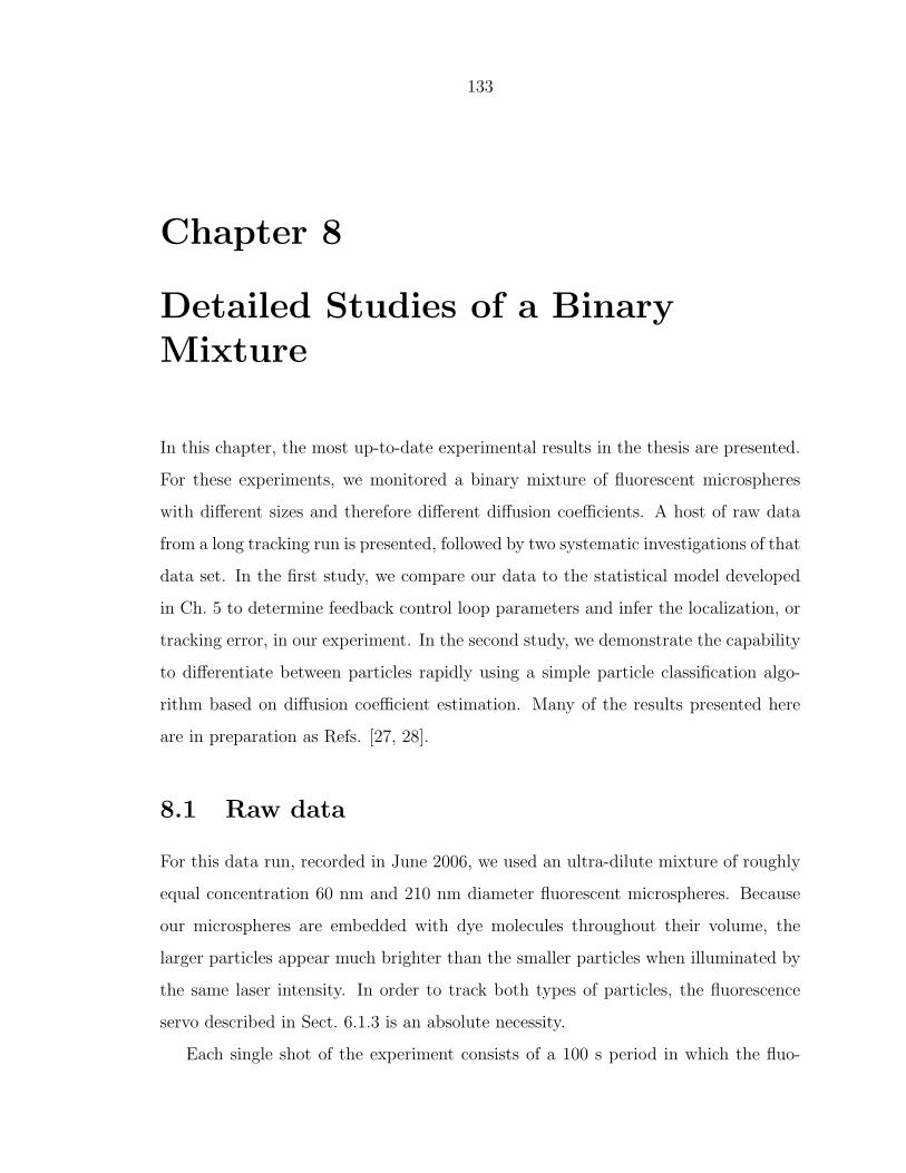
133

Chapter 8

Detailed Studies of a BinaryMixture

In this chapter, the most up-to-date experimental results in the thesis are presented.

For these experiments, we monitored a binary mixture of fluorescent microspheres

with different sizes and therefore different diffusion coefficients. A host of raw data

from a long tracking run is presented, followed by two systematic investigations of that

data set. In the first study, we compare our data to the statistical model developed

in Ch. 5 to determine feedback control loop parameters and infer the localization, or

tracking error, in our experiment. In the second study, we demonstrate the capability

to differentiate between particles rapidly using a simple particle classification algo-

rithm based on diffusion coefficient estimation. Many of the results presented here

are in preparation as Refs. [27, 28].

8.1 Raw data

For this data run, recorded in June 2006, we used an ultra-dilute mixture of roughly

equal concentration 60 nm and 210 nm diameter fluorescent microspheres. Because

our microspheres are embedded with dye molecules throughout their volume, the

larger particles appear much brighter than the smaller particles when illuminated by

the same laser intensity. In order to track both types of particles, the fluorescence

servo described in Sect. 6.1.3 is an absolute necessity.

Each single shot of the experiment consists of a 100 s period in which the fluo-

134

20 40 60 800

5

10

10 20 30 40 50 60 70 80 900

20

40

60

Time [s]

Po

siti

on

[µ

m]

Co

un

ts/m

s

Figure 8.1: Data from a single shot of the binary mixture experiment. The upperplot shows the rate of photon detections. In the lower plot, the upper curves are thex and y positions of the sample stage during the same trajectory. The lower curve onthe lower plot shows the excitation laser power (in arbitrary units) required to lockthe number of detected photons to 5600 s−1. Three regions are discernible, in whichno particle is present (until 17 s), a 60 nm diameter particle is tracked (until 74 s)and a 210 nm diameter particle is tracked (until 90 s).

rescence photon arrival times, x and y positions of the piezoelectric stage, and the

excitation laser power are recorded. The data is then written to the computer hard

drive, and after a brief pause, the process is repeated. Details of the apparatus are

given in Ch. 6.1. Analog integrators were used as controllers, and the microcontroller

was programmed to monitor the piezoelectric stage position and send a digital reset

pulse whenever the stage reaches its boundaries at 0 and 100 µm. The reset pulse

triggers a switch that grounds both integrators, bringing the sample stage back to a

centered position (determined by a DC offset on the high voltage amp) and discarding

any currently tracked particle in the process.

Data from a single shot of the experiment is shown in Fig. 8.1. In that particular

run, the apparatus tracked a 60 nm particle for about 55 s before colliding with a 210

nm particle. Upon incidence of the larger (brighter) particle, the fluorescence servo

135

0 10 20 30 40 50 600

5

10

Cou

nts/

ms

0 10 20 30 40 50 600

50

100

∆t [s]

Posi

tion

[µm

]

Figure 8.2: Another trajectory from the same data set as Fig. 8.1. One axis of thepiezoelectric stage reached 0 µm at t = 45 s, which triggered the controller resetprocedure, ending the trajectory and discarding the tracked particle as the samplestage was reset to its center.

automatically cut the laser power, effectively rendering the smaller (dimmer) particle

invisible. Because of the asymmetric visibility of the particles (the bright particles are

visible when a dim one is being tracked at high laser power, but not vice versa), the

apparatus preferentially tracks 210 nm particles. However, at our extremely dilute

concentrations, these particle “collisions” are fairly rare. We observed only 3 such

events in a data set containing 62 total trajectories recorded over a few hours. Another

example tracking trajectory showing the controller reset procedure is displayed in Fig.

8.2.

To analyze the data, we inspected 44 shots of the experiment (4400 s of data)

and found 62 individual tracking trajectories. For example, for the data shown in

Fig. 8.1, we (conservatively) labeled one trajectory as extending from 20 to 70 s and

another trajectory from 75 s to the end of the run. For this data set, no trajectories

ended with the loss of a particle due to a tracking failure; each trajectory ended

either at a particle collision, or at the boundary of the tracking region. We only

analyzed trajectories of at least 10 s duration, and of course the maximum trajectory

length was 100 s when a particle was tracked for the entire recording period. Having

136

partitioned the data into an ensemble of individual particle trajectories, we are able to

analyze the data efficiently. Among other quantities, the diffusion coefficient estimate

D∆t, the sample stage velocity autocorrelation function 〈∆X∆t(t)∆X∆t(t+ τ)〉, and

the fluorescence autocorrelation function g(τ) were calculated from the data. The

excitation laser power required to lock the particle’s fluorescence to 5.8 kHz was also

recorded, and provides a measure of a particle’s brightness since a brighter particle

requires less power to reach the same fluorescence intensity. These and other statistics

are displayed in Figs. 8.1-8.12 and discussed in the figure captions.

137

0 1 2 3 4 5 6 7 80

2

4

6

8

10

D [∆ t=0.2 s]

Num

ber

of o

ccur

ence

s

Figure 8.3: Histogram of observed diffusion coefficients D∆t with ∆t = 0.2 s. Thedistribution is clearly bimodal, with the 210 nm particles clustered around the meanvalue 1.3 µm2/s and 60 nm particles clustered at 5.4 µm2/s. For this and subsequentplots, we color code each individual data point as red (210 nm diameter) or blue (60nm diameter) according to this histogram.

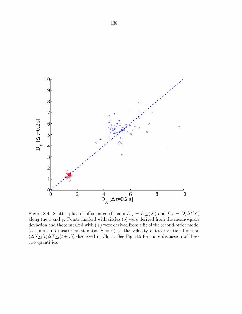
138

0 2 4 6 8 100

1

2

3

4

5

6

7

8

9

10

DX

[∆ t=0.2 s]

DY

[∆

t=0.

2 s]

Figure 8.4: Scatter plot of diffusion coefficients DX = D∆t(X) and DY = D)∆t(Y )along the x and y. Points marked with circles (o) were derived from the mean-squaredeviation and those marked with (+) were derived from a fit of the second-order model(assuming no measurement noise, n = 0) to the velocity autocorrelation function〈∆X∆t(t)∆X∆t(t+ τ)〉 discussed in Ch. 5. See Fig. 8.5 for more discussion of thesetwo quantities.

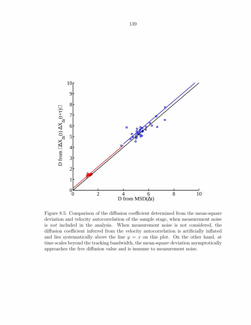
139

0 2 4 6 8 100

1

2

3

4

5

6

7

8

9

10

D from MSD(∆t)

D f

rom

⟨ ∆X

∆t(t

) ∆X

∆t(t

+τ)

⟩

Figure 8.5: Comparison of the diffusion coefficient determined from the mean-squaredeviation and velocity autocorrelation of the sample stage, when measurement noiseis not included in the analysis. When measurement noise is not considered, thediffusion coefficient inferred from the velocity autocorrelation is artificially inflatedand lies systematically above the line y = x on this plot. On the other hand, attime scales beyond the tracking bandwidth, the mean-square deviation asymptoticallyapproaches the free diffusion value and is immune to measurement noise.

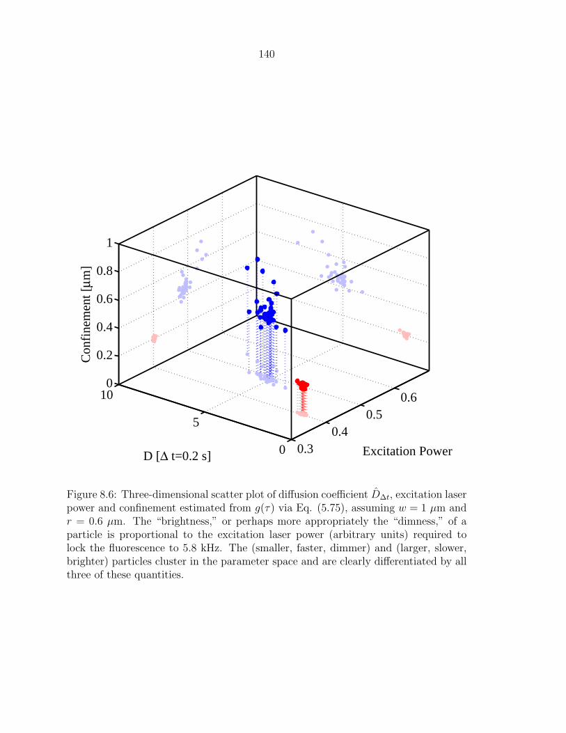
140

0.30.4

0.50.6

0

5

100

0.2

0.4

0.6

0.8

1

Excitation PowerD [Δ t=0.2 s]

Con

fine

men

t [μm

]

Figure 8.6: Three-dimensional scatter plot of diffusion coefficient D∆t, excitation laserpower and confinement estimated from g(τ) via Eq. (5.75), assuming w = 1 µm andr = 0.6 µm. The “brightness,” or perhaps more appropriately the “dimness,” of aparticle is proportional to the excitation laser power (arbitrary units) required tolock the fluorescence to 5.8 kHz. The (smaller, faster, dimmer) and (larger, slower,brighter) particles cluster in the parameter space and are clearly differentiated by allthree of these quantities.

141

0 10 20 30 40 50 60 70 80 90 100

0.4

0.45

0.5

0.55

Tracking time [s]

Exc

itatio

n Po

wer

[A

.U.]

Figure 8.7: Excitation laser power versus total tracked time. Note that the brighter(210 nm) particles are tracked within the allowable duration (10 to 100 s) with anearly uniform distribution. On the other hand, the dimmer (60 nm) particles weremore likely to be tracked for shorter times. This effect is due to both the preferentialtracking of 210 nm particles and the simple fact that the smaller, faster moving par-ticles reach the sample boundaries and trigger the tracking controller reset sequencemore often that the slower particles. Trajectory lengths for the 60 nm particles werediscussed in Sect. 7.3.

142

0 1 2 3 4 5 6 7 8500

600

700

800

900

1000

1100

1200

1300

1400

D [Δ t=0.3 s]

Cou

nts/

10 m

s

Figure 8.8: The standard deviation (RMS) value (+) of the fluorescence photoncount rate recorded during tracking along with and the expected value from Poissonstatistics at the same average rate (o) are plotted against the diffusion coefficient. The“sub-shot-noise” values are not a violation of classical statistics, but are a result ofthe fluorescence servo’s ability to control fluorescence fluctuations at slow timescales.

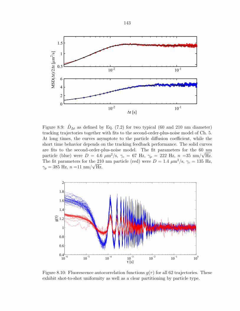
143

0.5

1

1.5

10-2 10-10

2

4

6

∆t [s]

10-2 10-1

MSD

(∆t)/

2∆t [

µm2 /s

]

Figure 8.9: D∆t as defined by Eq. (7.2) for two typical (60 and 210 nm diameter)tracking trajectories together with fits to the second-order-plus-noise model of Ch. 5.At long times, the curves asymptote to the particle diffusion coefficient, while theshort time behavior depends on the tracking feedback performance. The solid curvesare fits to the second-order-plus-noise model. The fit parameters for the 60 nmparticle (blue) were D = 4.6 µm2/s, γc = 67 Hz, γp = 222 Hz, n =35 nm/

√Hz.

The fit parameters for the 210 nm particle (red) were D = 1.4 µm2/s, γc = 135 Hz,γp = 385 Hz, n =11 nm/

√Hz.

10−6

10−5

10−4

10−3

10−2

10−1

100

0.4

0.6

0.8

1

1.2

1.4

1.6

1.8

2

τ [s]

g(τ)

Figure 8.10: Fluorescence autocorrelation functions g(τ) for all 62 trajectories. Theseexhibit shot-to-shot uniformity as well as a clear partitioning by particle type.

144

10−6

10−5

10−4

10−3

10−2

10−1

−0.2

0

0.2

0.4

0.6

0.8

τ [s]

g(τ)

Figure 8.11: Fits of g(τ) to the second-order-plus-noise model of Ch. 5 for two ofthe curves displayed in Fig. 8.10. We used w = 1 µm and D as determined fromthe mean-square deviation, as discussed in Table 7.1. For the 60 nm particle (blue),the parameters were r = 0.6, D = 5.0 µm2/s, γc = 127 Hz, γp = 291 Hz, n = 22nm/

√Hz. for the 210 nm particle (red), the parameters were r = 0.5, D = 1.3 µm2/s,

γc = 250 Hz, γp = 296 Hz, n = 15 nm/√

Hz.

145

0 100 200 300 400 5000

50

100

150

200

250

300

350

400

450

500

Bandwidth from g(τ) [Hz]

Ban

dwid

th f

rom

MSD

(∆t)

[H

z]

Figure 8.12: Comparison of feedback bandwidth parameters as determined from fitssuch as those in Figs. 8.11 and 8.9. The red points show the integrator bandwidthγc and the blue points show the low-pass Plant bandwidth γp. The color code isdifferent from previous figures! g(τ) tends to underestimate the integrator bandwidthγc relative to MSD(∆t), while the values of γp are commensurate across the separateanalyses.

146

0 5 10 15 20 25 300

20

40

60

80

100

n from g(τ) [nm/Hz1/2]

n fr

om M

SD(Δ

t) [

nm/H

z1/2 ]

Figure 8.13: Comparison of measurement noise n determined from fits such as thosein Figs. 8.11 and Fig. 8.9. Note the different scales on the axes, showing the largespread in n as determined from MSD(∆t).

147

8.2 Near-optimal tracking

In Ch. 4, we discussed in detail the limitations on particle localization that arise

from the fundamentally noisy fluorescence photon counting process. This optical

shot-noise tracking limit imposes the constraint that a diffusing particle cannot be

tracked arbitrarily well at a finite fluorescence count rate, since an overly aggressive

feedback controller will feed photon counting noise back into the system [26]. In this

section, we use our statistical tracking model and the large data set displayed in Figs.

8.3-8.12 to make quantitative inferences about particle localization during tracking

in our experiment. We will see that in some cases we approach quite close to the

shot-noise limit.

In particular, we will assume the second-order-plus-noise model of Ch. 5 and use

the mean-square deviation MSD(∆t) and the fluorescence autocorrelation function

g(τ) to determine the system parameters D, γc, γp and n in two separate ways. From

Sect. 5.1.4, we know that the steady-state tracking error for our second-order system

with these parameters is

L =√

E [E(t)2] =

√D

(1

γc

+1

γp

)+n2γc

2. (8.1)

Having found these parameters by curve fitting to our data, we may then extract each

particle’s localization using Eq. (8.1). The resulting values of L are plotted versus

the measured diffusion coefficient D in Fig. (8.14). In order to confirm the validity of

this curve fitting technique for estimating L, we generated Monte Carlo simulations of

the second-order control system model driven by particle diffusion and measurement

noise, using typical values of the parameters n, γc, γp, and D. We then estimated L

and D on the resulting “data” using the mean-square deviation, and these results are

shown in gray in Fig. 8.14. The 60 nm beads are more poorly localized, due to their

faster diffusion, and the inference of L from mean-square deviation data is also much

more prone to noise for these particles, as seen from the large spread in inferred L

values for the Monte Carlos simulations.

148

0 1 2 3 4 5 6 7 80

0.5

1

1.5

D [μm2/s]

Loc

aliz

atio

n [μ

m]

Figure 8.14: Inferred localization L versus D for 62 individual tracking trajectories(dark circles). The lighter circles are the results of simulations described in the text.The dashed line is the localization limit based on optical shot noise. Typical fitparameters for the 210 nm beads (red) are D = 1.3µm2/s, n = 15 nm/

√Hz, γc = 111

Hz, γp = 343 Hz. The localization values marked by (+) were determined from g(τ)with the value of D set from the tracking data and assuming w = 1 µm, but thelocalization determined from g(τ) is fairly robust to the choice of w.

Values of L inferred from fits to g(τ) with D determined from the mean-square

deviation are also shown in Fig. 8.14, and these appear much more robust to the data

analysis procedure. Note that for the 60 nm particles, the localization values deter-

mined from g(τ) are more tightly clustered than those determined from MSD(∆t).

As with all fluorescence autocorrelation methods, the length scale is set by the beam

waist w, which we must calibrate separately, however the inferred values of the local-

ization are fairly robust to variations in w and tend to depend more strongly on the

beam shape through r/w and on the damping parameters γc and γp.

The dashed line in Fig. 8.14 is the shot-noise localization limit derived in Ch. 4 for

our experimentally determined values of the beam waist w = 1 µm, rotation radius

r = 0.6 µm and maximum fluorescence count rate at the peak laser intensity, Γ0. Γ0

was inferred from the beam parameters w and r, the localization L, and the observed

149

0

0.5

1

1.5

00.5

11.50

0.5

1

1.5

L from g(τ)

L from MSD(Δ t)

L f

rom

g0

Figure 8.15: Comparison of the localization L determined from MSD(∆t), g(τ), andg0.

(average) fluorescence intensity 〈Γ〉, which are related by

〈Γ〉 =Γ0w

2

(w2 + 4L2)exp

[2r2

(w2 + 4L2)

]. (8.2)

For the 210 nm particles we find Γ0 = 9.8 kHz and for the 60 nm particles we find

Γ0 = 15.1 kHz. The shot-noise localization limit in this case is given by combining

Eqs. (4.12) and (4.18b) to find

Lmin =

√w2

r

√D

4Γ0

exp

(r2

w2

). (8.3)

Finally, we can also estimate the localization L from autocorrelation functions

near g(τ = 0) = g0, as in Eq. (5.75). This fit requires the values of w and r which we

take to be 1.0 and 0.6 µm, respectively. A comparison of L determined in all three

different ways is shown in Fig. 8.15.

Our results for the localization L as determined by all of these different methods

are summarized in Tables 8.1 and 8.2. MSD(∆t) is simply not very sensitive to the

measurement noise n for the 60 nm particles as evident from the standard deviation

150

210 nm particles

L [nm]

n [nm/√

Hz]

MSD(∆t) g(τ) g0 Opt.169± 21.2 143± 40 204± 10 11715.4± 5.4 6.3± 6.5 – 9.4

Table 8.1: Table comparing the localization and measurement noise determined fromMSD(∆t), g(τ), and g0 for the 210 nm diameter particles. Shot-noise limited optimalvalues are denoted by “Opt.” The error values are the standard deviation in observedparameters.

of this parameter. This is because the measurement noise contributes at small time

scales, while the mean-square deviation is sensitive all the way out to very long times

where it asymptotically approaches the diffusion coefficient D. On the contrary, g(τ)

tends to be extremely sensitive to short timescales; after all, we can measure it deep

into the sub-µs range. However, g(τ) damps away at the feedback timescale and is

not particularly sensitive to long-time statistics. As a result, when we determine D

from the mean-square deviation at long times and insert this into g(τ) in order to

find n at short times, we find tightly constrained and high quality results.

8.3 Classification by diffusion coefficient estima-

tion

In this section, we consider an application of closed-loop particle tracking in which

we classify particles as small (60 nm diameter) or large (210 nm diameter) according

to an estimate of the diffusion coefficient. In particular, we want to know just how

much data is required to make classifications with a specified error rate. The problem

requires a good statistical description of the system, which we have spent a lot of

time and effort developing and confirming in preceding sections. We will see that

classifications can be made with very little data and with a very simple algorithm

that could easily be implemented in real-time, offering the tantalizing possibility

of triggering an event, such as a microfluidic pressure pulse for steering a particle

or a photocatalytic laser flash for initiating a chemical reaction, using fast particle

classification. In this binary scenario, we achieve 90% success rates on the basis of only

151

60 nm particles

L [nm]

n [nm/√

Hz]

MSD(∆t) g(τ) g0 Opt.611± 359 340± 41 481± 79 150152± 190 18.0± 6.2 – 7.3

Table 8.2: Table comparing the localization and measurement noise determined fromMSD(∆t), g(τ), and g0 for the 60 nm diameter particles. Note the unnacceptablylarge spread in the measurement noise n determined from MSD(∆t) for these parti-cles. As discussed in the text, the values of L determined from g(τ) are consideredthe most reliable here because they rely on the sensitivity of g(τ) at short times andMSD(∆t) at long times (through the diffusion coefficient D).

∼600 detected photons collected over 120 ms, and our counting rates and diffusion

coefficients are comparably to those of fluorescent proteins in a cellular environment.

8.3.1 Statistics of D∆t

We now return to the basic problem of diffusion coefficient estimation, which has

already been discussed on a few separate occasions. We will begin by explicitly

defining our estimators, because we will also want to know their distributions. During

tracking, we measure the coordinates X(t) and Y (t) of a particle by recording the

x and y positions of the sample stage. We can form an estimate of the diffusion

coefficient along each direction by calculating the variance in the trajectory step size

over N time intervals of length ∆t, where the choice of N and ∆t will determine the

statistical accuracy of the estimate as well as the total estimation time T = N∆t.

Let

∆X∆t(k) = X [(k + 1)∆t]−X [k∆t] (8.4)

be the change in the particle’s position over the kth time interval of length ∆t, a

slight modification of the earlier definition. X(t), T , ∆t, and ∆X∆t are shown for an

individual trajectory in Fig. 8.17. With N samples, we may estimate the mean µ

152

1 2 3 4 5 6 7 8 90

1

2

3

4

5

6

7

8

Estimation time [s] (∆ t = 0.1 s)

D [

µm2 /s

]

0 500

1

2

3

4

5

6

7

8

Figure 8.16: Convergence of D∆t as the number of samples is increased by increasing∆t. Only the first 10 trajectories of fast (60 nm diameter) and slow (210 nm diameter)tracked beads are shown on the left for clarity. Underneath is a a colorized contourplot of the distribution pN(D;D) given by Eq. (8.9). At the right, the final value ofthe estimate (at T = 10 s) is shown for the entire data set, together with the expecteddistribution based on χ2 statistics. The solid curves on the right have only one freeparameter, the diffusion coefficient D.

and variance σ2 of ∆X∆t by

µ∆t(X) =1

N

N∑k=1

∆X∆t(k) (8.5a)

σ2∆t(X) =

1

N − 1

N∑k=1

[∆X∆t(k)− µ∆t(X)]2 (8.5b)

and form an unbiased estimator of the diffusion coefficient D with

D∆t(X) =1

2∆tσ2

∆t(X). (8.6)

The normalization byN−1 in σ2∆t(X) defined by Eq. (8.5) gives an unbiased estimate,

canceling the contribution to the variance arising from error in the estimated mean

[58]. We could have used other prefactors: normalization by N gives the sample vari-

153

30 40 50 60 70 80 90

20

40

60

80

100

t [s]

Sta

ge

Po

siti

on

[µ

m]

∆t

T

∆X∆t

t0 t1

X(t)

tN...

Particle enters

X(t)

Y(t)

30 40 50 60 70 80 900

2

4

6

8

10

Co

un

ts [

kH

z]

t [s]a) b)

Figure 8.17: Typical trajectory of a single tracked particle. The main plot showsthe coordinates X(t) and Y (t) of the sample stage. A particle enters the focus neart = 47 s and is tracked for the remainder of the data run. Inset (a) shows a T = 2 sportion of X(t), illustrating T , ∆t, ∆X∆t and N as used in the text. Inset (b) showsthe fluorescence photon count rate during the same trajectory.

ance (as distinct from the variance of the underlying distribution), and normalization

by N + 1 gives the estimate of the sample variance with the minimum mean-square

error. For large N these distinctions become negligible. Estimates of µ, σ2 and D

from two-dimensional data are simply formed by averaging the quantities µ∆t, σ2∆t,

and D∆t along each Cartesian direction. Whenever we do not include the argument

X or Y in these quantities, it is implied that they are calculated in two dimensions.

Other estimators of D exhibiting varying convergence rate, bias, and computational

complexity may be defined [3, 21], but we have chosen D∆t specifically for its ease of

implementation and consequent potential for future real-time applications.

When the measured trajectories X(t) and Y (t) represent pure Brownian motion

with drift velocity v and diffusion coefficient D, the estimators µ∆t and σ2∆t have

154

expectation values

E [µ∆t(X)] = v∆t (8.7a)

E[σ2

∆t(X)]

= 2D∆t (8.7b)

E[D∆t(X)

]= D (8.7c)

with the same results for Y . The last line shows that D∆t is an unbiased estimator

of D. In contrast to many of the other quantities we have consider thus far, the

estimate D∆t is not a Gaussian random variable, rather its distribution is given by

the χ2 distribution with N − 1 degrees of freedom [58]. This is of course a standard

fact concerning the distribution of the sample variance of a Gaussian process. The

cumulative density (FN) and probability density (fN) of the χ2 distribution, with N

degrees of freedom, are given by

FN(x) =γ(N/2, x/2)

Γ(N/2)(8.8a)

fN(x) =∂

∂xFN(x) =

2−N/2

Γ(N/2)xN/2−1e−x/2 (8.8b)

where Γ(N) and γ(x,N) are the gamma function and incomplete gamma function,

respectively [59].1 Define pN(D;D) to be the probability density for our estimate D∆t

to assume the value D. Then we find

pN(D;D) =N − 1

DfN−1

(N − 1

DD

). (8.9)

The corresponding cumulative density function PN(D;D) is given by

PN(D;D) =

∫ D

0

pN(x;D)dx = FN−1

(N − 1

DD

). (8.10)

The distributions pN(D;D) and PN(D;D) depend only on the underlying diffusion

1Be careful with the incomplete gamma function, because it is defined differently in Matlab,Mathematica, and Abramowitz and Stegun [59], whose definition and notation we use here.

155

10-3

10 -2

10 -10

2

4

6

∆t [s]

D∆

t [µ

m2 /

s]

Figure 8.18: Diffusion coefficient estimate D∆t as ∆t is varied over the tracked tra-jectory of a 60 nm (red squares) and 210 nm (blue circles) diameter fluorescent mi-crosphere. At small ∆t, the estimate D∆t is smaller than the asymptotic value dueto the finite tracking bandwidth.

coefficient D and the number of samples N ; they do not depend explicitly on the time

interval ∆t at which the trajectory is sampled. However, for fixed overall estimation

time T , a smaller ∆t allows more samples in that interval. Assuming that the mea-

surement interval T is broken up into an integer number of sample times ∆t, we have

N = T/∆t.

The value of D∆t (with T equal to the total tracking time) is shown in Fig. 8.18

as a function of ∆t, for a measured trajectory of each type of particle. As detailed

in Ch. 5, D∆t underestimates the particle’s diffusion coefficient at small ∆t due to

the finite response bandwidth of the feedback loop. Qualitatively, this effect arises

because our piezoelectric stage cannot move sufficiently fast to track the particle’s

motion at arbitrarily small timescales, and of course this effect is a generic feature

of all realistic control systems. For pure (uncontrolled) Brownian motion, the step

sizes ∆X∆t obey Gaussian statistics and the estimate D∆t obeys χ2 statistics with

mean value D [58]. Because our feedback control system is linear, D∆t still obeys χ2

statistics even for small ∆t, albeit with a value of D that is below the asymptotic

156

15253545

012345

0

0.5

1

1.5

D∆t [µm2/s]

N

Figure 8.19: Histogram of the estimate D∆t for ∆t = 10 ms (indicated by dark circlesin Fig. 8.18) versus the number of samples N used for the estimate. The solid blackcurves show the expected distribution pN(D;D) with mean value D set equal to themean value from each data set.

value. This fact is confirmed in Fig. 8.19, where we show the full distribution of D∆t

for ∆t = 10 ms and varying numbers of samples N .

8.3.2 Hypothesis testing

Now consider a binary mixture of particles, such as the one used for our measurements,

consisting of a fraction λ1 of particles of type 1 (diffusion coefficient D1) and a fraction

λ2 = 1−λ1 of particles of type 2 (diffusion coefficient D2 ≥ D1). We now wish to find

a threshold value of the diffusion coefficient Dth such that we may assign a particle

to class 1 if D∆t < Dth and class 2 for D ≥ Dth. Let Pcorr denote the probability that

a classification is correct under this thresholding algorithm. For any given threshold

value Dth, the probability of a correct classification is

Pcorr = λ1PN (Dth;D1) + λ2 [1− PN (Dth;D2)] , (8.11)

157

and straightforward calculation shows that, the value of Pcorr is maximized by choos-

ing the threshold value

Dth = D∗th =

D1D2

D2 −D1

(log

D2

D1

+2

N − 1log

λ1

1− λ1

). (8.12)

D∗th is a weak function of λ1 and N for even moderately large N , and if λ1 = λ2, i.e.,

if the particles occur with equal likelihood (or we have no prior knowledge of their

distribution), then D∗th does not depend on N at all. D∗

th given by Eq. (8.12) may

become negative or unbounded, but these limits simply indicate regimes in which the

measurement is too noisy to warrant any correction to the prior distribution.

In a more general scenario, particle classification based on a measurement record

may be formulated as a problem of hypothesis testing [58]. In the binary form of this

problem, an m-component measurement is made with result θ, which may represent

a single measurement or it a sequence of measurements. The experimenter knows

that this measurement results was drawn from one of two distributions, p1(θ) and

p2(θ) with corresponding probabilities λ1 and λ2 = 1−λ1, and wishes to decide which

of these distributions was most likely to have produced the observed value. Let H1

represent the hypothesis that the underlying distribution was p1(θ) and similarly for

H2. Then we define a test procedure by the following threshold criterion: we accept

hypothesis H1 if λ1p1(θ) > λ2p2(θ), and reject it otherwise. A standard theorem

states that this test procedure minimizes the probability of an incorrect classifica-

tion; furthermore, the Neyman-Pearson Lemma states that any other test procedure

that decreases the probability of incorrectly accepting H1 necessarily increases the

probability of incorrectly accepting H2 [58]. For our specific case of particle classifi-

cation based on the scalar estimate D∆t, the test described above divides the positive

real line into regions corresponding to particles of type 1 (D∆t < D∗th) and type 2

(D∆t ≥ D∗th) where D∗

th is simply the point where

D∗th : λ1pN(D∗

th;D1) = λ2pN(D∗th;D2), (8.13)

158

10-2

10 -1

100

1010.5

0.6

0.7

0.8

0.9

1

T [s]

P corr

∆t = 0.01 s∆t = 0.05 s∆t = 0.1 s∆t = 0.5 s

Figure 8.20: Measured probability of correct classification Pcorr as the estimation timeT and the sample time ∆t are varied. The dashed curves show the expected successprobability from Eq. (8.11).

exactly as defined in Eq. (8.12). This general formulation can be applied to the case

of a two-dimensional estimate of diffusion coefficients Dx and Dy along two Cartesian

directions, even for the case that these are not identically distributed, i.e., the diffu-

sion is not isotropic. In that case, the measurement vector θ =[D∆t(X) , D∆t(Y )

]lies in a Dx-Dy plane, and the threshold criterion is a line dividing the plane into

regions corresponding to each type of particle. For higher-dimensional measurement

vectors, the hypothesis testing criterion is a surface partitioning the measurement

space into regions corresponding to H1 and H2.

8.3.3 Results

We implemented the above classification procedure on the first 48 individual tracking

trajectories from our data set, with various values of T , ∆t and N . We usually

form our estimate using short segments of very long trajectories, so we may confirm

whether a particular estimate based on a sample of length T correctly identified a

particle by comparing it to a high-fidelity identification using data from the entire

trajectory. In this way, we retain the ability to calculate the success probability, Pcorr.

159

Figure 8.21: Pcorr for ∆t = 10 ms as the threshold Dth and number of samples Nare varied. The observed values are shown as blue circles while the solid lines isthe expected value based on Eq. (8.11). From the figure, we find that the derivedvalue of D∗

th that maximizes Pcorr also maximizes the observed classification successprobability.

The results are shown in Fig. 8.20. At fixed estimation time T , Pcorr strictly increases

with decreasing ∆t down to about 10 ms. At shorter times, our particles move (on

average) only 250–500 nm, comparable to the localization values L determined in

Sect. 8.2, and we are no longer able to make fast determinations of position with the

accuracy required to form a good estimate D∆t.

At T = 60 ms we collect only (on average) 275 fluorescence photons but still

identify particles with >75% success; over this interval the larger 210 nm particles

move on average only 600 nm, while the smaller 60 nm particles move only 1150 nm.

When the observation time is doubled to T = 120 ms, the success rate reaches 90%.

At T = 1 s, the success rate is >99% and even the faster (60 nm) particles move

less than 5 µm. We emphasize that these success rates are essentially limited by the

tracking error and feedback bandwidth, which are in turn nearly limited by photon

counting shot noise as shown in Sect. 8.2.

Although we derived the optimal value of the threshold D∗th for particle classifica-

tion, we may still the test the optimality of this threshold in our data. In Fig. 8.21, we

160

show the probability of a correct classification Pcorr given by Eq. (8.11) with ∆t = 10

ms, as N and Dth is varied. The figure shows that even for small N where the ob-

served value of Pcorr falls away from the expected value, the optimum classification

threshold remains very near D∗th.

Note that since individual particles are tracked for times much longer than are

required for accurate characterization, our method could be used to detect real-time

changes in the diffusive behavior of an individual particle caused, e.g., by binding

events or conformational switching in the case of a single biomolecule.

8.4 Summary and commentary

Throughout this chapter, we drew on the theoretical apparatus developed in Chs. 2-

5 to demonstrate the full quantitative capability of closed-loop particle tracking for

localizing and monitoring fluorescent Brownian particles. Our purpose has been not

only to demonstrate the experimental capability for such feedback-assisted control,

but also to give a unified description of the apparatus in the most natural language,

that of linear stochastic control theory. We have now shown that such an analysis can

describe and predict the response of the apparatus in terms of the transfer functions

of its components and the inferred or derived measurement noise. We understand

the fluctuations in a particle’s fluorescence in terms of the competition between free

diffusion and tracking control; we have demonstrated the nearly optimal localization

of particles by analyzing the controller response and also examining the fluorescence

fluctuations. Finally, we applied many of these methods to the task of performing

real-time particle classification with high fidelity based on very few photons collected

over small spatial scales that should carry over with direct applicability to experiments

involving single quantum dots or fluorescent biomolecules.

The future of this project offers interesting and exciting prospects both for tech-

nical and scientific development. The results presented throughout this thesis fully

characterize the tracking system, with the theoretical apparatus in no way restricted

to the measured two-dimensional tracking results. Our surprising capability to track

161

10-2

10-1

100

101

102

103

104

105

D [µm2/s]

Γ [s

-1] This work

Trackin

g diff

iculty

Membrane proteins

Membrane lipids

Chen et al.

Rhoades et al.

Figure 8.22: Plot of the D-Γ parameter space for values relevant to single-moleculebiophysics; contours of constant “trackability” D/(Γw2), with w fixed, are shown assolid black lines. D and Γ for EGFP (a fluorescent protein) in the cellular cytoplasm,nucleus, and free in solution (blue squares, from left to right respectively) were takenfrom Chen et al. [60]; the brightness of individual vesicle-immobilized, FRET-labeledadenylate kinase molecules, shown as a horizontal line labeled by “Rhoades et. al,”was taken from Ref. [61]; approximate diffusion coefficients for lipids and proteinsintegrated into a cell membrane are shown as dashed vertical lines, taken from Ref.[62]. The results from this chapter are shown as red circles, and the lighter shadedarea represents the region of parameter space where single-molecule tracking presentsno technical challenge beyond the results in this thesis.

the two-dimensional motion of fast moving particles at fluorescent count rates as low

as 5 kHz with tracking errors approaching the photon counting shot-noise limit, gives

me great confidence that these techniques can reach a very exciting target in the near

future: we can extend the tracking into three dimensions, with the straightforward

addition of a third axis of fluorescence modulation and tracking control, and track

a single fluorescent protein molecule in free solution. The feasibility of this goal can

be investigated using the general tracking considerations in Ch. 4. In that chapter,

we saw that fundamental noise processes limit the “trackability” of a particle with

diffusion coefficient D and fluorescent count rate Γ in a Gaussian laser with beam

waist w. The difficulty of tracking a particle can be encapsulated in the dimensionless

162

parameter D/(Γw2), meaning brighter or, equivalently, slower-moving particles are

easier to track than dim, fast ones (at fixed w).

In Fig. 8.22, the diffusion coefficient D is plotted versus the fluorescent count

rate Γ for our results, and some important regions of the parameters space relevant

to single-molecule biophysics are indicated as well. We see from the figure that our

results are already consistent with the technical requirements for tracking individ-

ual EGFP proteins in a cellular environment. Furthermore, an increase of our beam

waist by a factor of 2 (to w ≈ 2 µm) should bring EGFP in free solution (the blue

point in the upper right of Fig. 8.22) into our accessible parameter regime, with a

corresponding loss of spatial resolution. In order to reach these goals, we must move

to three-dimensional tracking in order to remove the final “perturbative” aspect of

our experiment, the nearby glass cover-slips. Such a move into three-dimensions is

already in progress; it requires the addition of a third axis for spatially modulating the

excitation laser along with a third piezo-electric stage and controller. The achieve-

ment of our protein-tracking benchmark will complete the technical development of

the closed-loop particle tracking microscope and open an era of single-molecule fluo-

rescence spectroscopy in which the noise sources discussed in Ch. 1 will be suppressed

to the maximum extent allowed by fundamental processes such as photon counting

statistics and Brownian motion.

163

Appendix A

Closed-Loop CorrelationSpectroscopy with Internal StateTransitions

In chapter 5, we developed a theory to describe the fluctuations in a tracked (or

trapped) particle’s fluorescence arising from deterministic laser motion and partially

controlled transverse diffusion, and in Chs. 6-8 we saw that the theory agrees quite

well with experiment. It is the aim of this appendix to extend that theory to include

linearized chemical reaction kinetics, in a manner analogous to the original theory

of (open-loop) FCS [6–9]. These reaction kinetics take the form of internal state

transitions that affect the diffusion and fluorescence properties of the particle. Some

results along these lines have been obtained by Monte Carlo simulation of a similar

system in [13].

Unlike the model in Ch. 5, we will not be able to solve the general form of the

problem presented here. We will concentrate on the case that the particle has n = 2

internal states and the feedback control is first order. We will find some approximate

results for the case when dynamical timescales are well separated and an adiabatic

elimination procedure is available, and we will find an exact solution for the special

case that state transitions do not affect the particle’s steady-state diffusion statistics.

Finally, we will give a solution in the form of an eigenfunction expansion for the gen-

eral two-state problem that hides the complexity of the results in infinite-dimensional

matrices. There is certainly room for more theoretical development of these ideas,

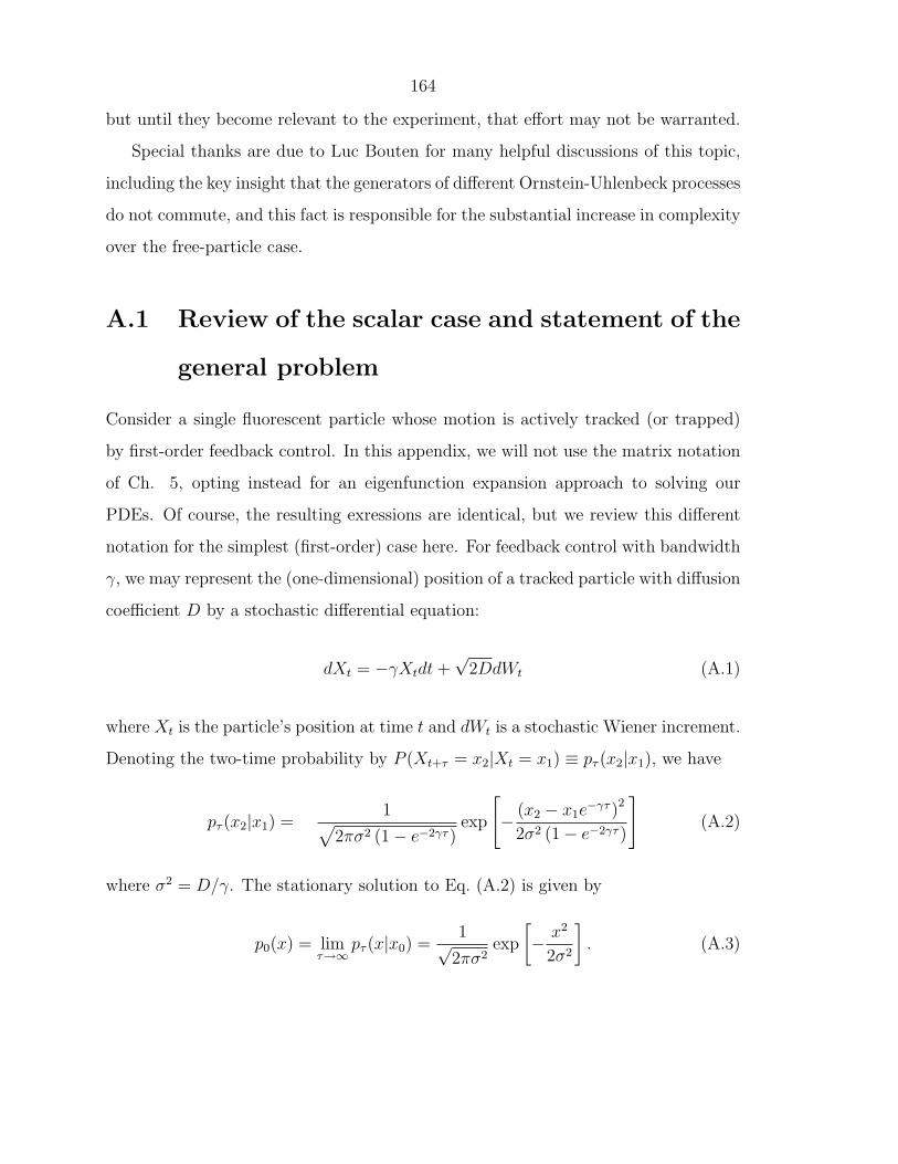
164

but until they become relevant to the experiment, that effort may not be warranted.

Special thanks are due to Luc Bouten for many helpful discussions of this topic,

including the key insight that the generators of different Ornstein-Uhlenbeck processes

do not commute, and this fact is responsible for the substantial increase in complexity

over the free-particle case.

A.1 Review of the scalar case and statement of the

general problem

Consider a single fluorescent particle whose motion is actively tracked (or trapped)

by first-order feedback control. In this appendix, we will not use the matrix notation

of Ch. 5, opting instead for an eigenfunction expansion approach to solving our

PDEs. Of course, the resulting exressions are identical, but we review this different

notation for the simplest (first-order) case here. For feedback control with bandwidth

γ, we may represent the (one-dimensional) position of a tracked particle with diffusion

coefficient D by a stochastic differential equation:

dXt = −γXtdt+√

2DdWt (A.1)

where Xt is the particle’s position at time t and dWt is a stochastic Wiener increment.

Denoting the two-time probability by P (Xt+τ = x2|Xt = x1) ≡ pτ (x2|x1), we have

pτ (x2|x1) =1√

2πσ2 (1− e−2γτ )exp

[− (x2 − x1e

−γτ )2

2σ2 (1− e−2γτ )

](A.2)

where σ2 = D/γ. The stationary solution to Eq. (A.2) is given by

p0(x) = limτ→∞

pτ (x|x0) =1√

2πσ2exp

[− x2

2σ2

]. (A.3)

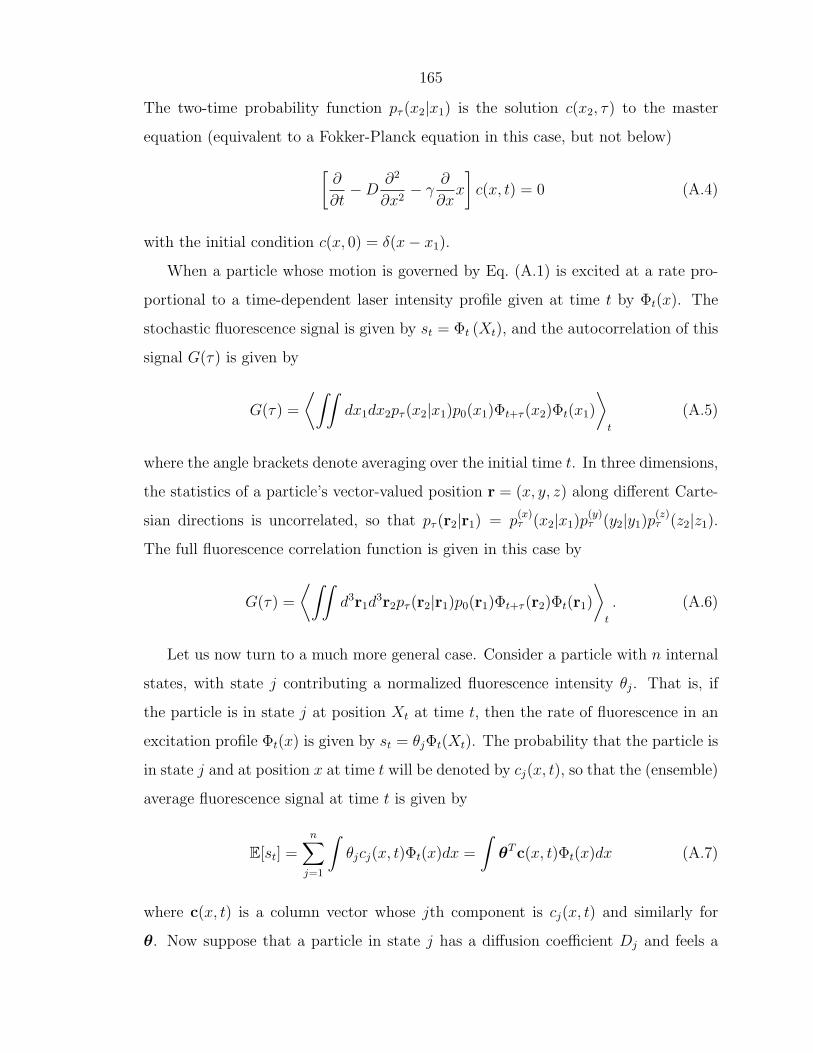
165

The two-time probability function pτ (x2|x1) is the solution c(x2, τ) to the master

equation (equivalent to a Fokker-Planck equation in this case, but not below)

[∂

∂t−D

∂2

∂x2− γ

∂

∂xx

]c(x, t) = 0 (A.4)

with the initial condition c(x, 0) = δ(x− x1).

When a particle whose motion is governed by Eq. (A.1) is excited at a rate pro-

portional to a time-dependent laser intensity profile given at time t by Φt(x). The

stochastic fluorescence signal is given by st = Φt (Xt), and the autocorrelation of this

signal G(τ) is given by

G(τ) =

⟨∫∫dx1dx2pτ (x2|x1)p0(x1)Φt+τ (x2)Φt(x1)

⟩t

(A.5)

where the angle brackets denote averaging over the initial time t. In three dimensions,

the statistics of a particle’s vector-valued position r = (x, y, z) along different Carte-

sian directions is uncorrelated, so that pτ (r2|r1) = p(x)τ (x2|x1)p

(y)τ (y2|y1)p

(z)τ (z2|z1).

The full fluorescence correlation function is given in this case by

G(τ) =

⟨∫∫d3r1d

3r2pτ (r2|r1)p0(r1)Φt+τ (r2)Φt(r1)

⟩t

. (A.6)

Let us now turn to a much more general case. Consider a particle with n internal

states, with state j contributing a normalized fluorescence intensity θj. That is, if

the particle is in state j at position Xt at time t, then the rate of fluorescence in an

excitation profile Φt(x) is given by st = θjΦt(Xt). The probability that the particle is

in state j and at position x at time t will be denoted by cj(x, t), so that the (ensemble)

average fluorescence signal at time t is given by

E[st] =n∑

j=1

∫θjcj(x, t)Φt(x)dx =

∫θTc(x, t)Φt(x)dx (A.7)

where c(x, t) is a column vector whose jth component is cj(x, t) and similarly for

θ. Now suppose that a particle in state j has a diffusion coefficient Dj and feels a

166

trapping force (or equivalently, a tracking bandwidth) characterized by γj. Suppose

also that the rate of transitions from state k into state j is a constant given by λjk.

Then the master equation governing the probability vector c(x, t) is

∂∂t −

F1 · · · 0...

. . ....

0 · · · Fn

−Λ

c(x, t) = 0 (A.8)

where

Fj = Dj∂2

∂x2+ γj

∂

∂xx (A.9)

is the (scalar) Ornstein-Uhlenbeck diffusion operator for state j and the matrix Λ

satisfies

Λjk = λjk , j 6= k (A.10a)

Λkk = −∑j 6=k

λjk. (A.10b)

Van Kampen [36] refers to Eq. (A.8) as governing a “composite Markov process,”

and gives a formal solution to the problem in terms of an inverse Laplace transform.

His solution is valid, however, only for the case where all of the diffusion operators

commute with each other (as is the case for free diffusion, the example he uses).

Unfortunately, the Ornstein-Uhlenbeck operators do not commute in general:

[Fj,Fk] = FjFk − FkFj = 2 (Djγk −Dkγj)∂2

∂x26= 0. (A.11)

In the n-dimensional case, assuming none of the parameters Dj and γj are zero,

then all operators commute only if D1/γ1 = D2/γ2 = · · · = Dn/γn; of course, this

is exactly the situation where the Ornstein-Uhlenbeck length-scales σ2j = Dj/γj are

all equal, so that internal state transitions do not affect the steady-state diffusion

statistics. For the remainder of this section, we will be concerned with solutions

of Eq. (A.8) and the resulting fluorescence autocorrelation functions for two-state

167

systems n = 2. Note also that the composite Markov process has been proposed as a

governing equation for very general processes in biophysics (as an example of an even

more general Smoluchowski equation) including DNA and protein folding kinetics

[63], and it also arises in financial models of market fluctuations.

A.2 The commuting case [F1,F2] = 0

As mentioned above, the diffusion operators Fk do not commute in general. However,

the special case that they do commute is not too trivial to give interesting and relevant

results. Let us now explicitly solve Eq. (A.8) for n = 2 assuming that D1γ2 = D2γ1

which ensures [F1,F2] = 0. We will develop solutions in terms of the eigenfunctions

of the diffusion operators defined by

F (k)n (x) ≡ Hn

(x√2σk

)exp

(− x2

2σ2k

)(A.12)

satisfying

FkF(k)n (x) = −nγkF

(k)n (x) (A.13)∫ ∞

−∞F (k)

n (x)F (k)m (x)dx =

(n!2n

√2πσ2

k

)δmn (A.14)

where δmn is the Kronecker delta. Hn(x) is the Hermite polynomial of order n [37].

Any square-integrable function f(x), including any spatial probability distribution,

may be expanded in the basis of these eigenfunctions

f(x) =∞∑

n=0

α(k)n F (k)

n (x) (A.15)

where the expansion coefficients are given by

α(k)n =

1√2πσ2

k

2−n

n!

∫ ∞

−∞dxHn

(x√2σ2

k

)f(x). (A.16)

168

We can drop the superscript (k) indicating the expansion basis because in this special

commuting case, the operators Fk share an eigenbasis. We now have σ22 = σ2

1 = σ2,

and only one basis of eigenfunctions Fn(x).

The solution to Eq. (A.8) can now be found by expanding an arbitrary initial state

in the eigenfunctions Fn(x) and calculating the time evolution of the nth component

directly. Let

Γ =

γ1 0

0 γ2

(A.17)

and let the initial state be given by

c(x, 0) =∞∑

n=0

αn

βn

Fn(x). (A.18)

Then the state at time t is given by

c(x, t) =∞∑

n=0

exp [(Λ− nΓ) t]

αn

βn

Fn(x) (A.19)

where the conditional dependence on the initial conditions has been omitted in the

notation. Let us now calculate the full fluorescence autocorrelation function (in one

dimension only) for this particle. Let cj2j1(x2, t2|x1, t1) be the probability to find the

particle at position x2 in state j2 at time t2, given that it was at position x1 and in

state j1 at time t1. This probability can be calculated using the solution defined in

(A.19). Now the full fluorescence autocorrelation function is given by

E[st+τst] =∑j1,j2

∫∫dx2dx1Φt+τ (x2)Φt(x1)θj2θj1cj2,j1(x2, t+ τ |x1, t)c

(0)j1

(x1) (A.20)

where c(0)j1

(x1) is he j1 component of the steady state solution. In a Gaussian excitation

laser whose centroid follows the (dimensionless) path xt/w = χt, we have

Φt(x) = exp

[−2( xw− χt

)2]. (A.21)

169

We may plug into Eq. (A.20) and perform the integrals to find

E[st+τst] =ζ exp

[−2ζ(χ2

t+τ + χ2t )]

(λ12 + λ21)

×∞∑

n=0

2−n

n!Hn

(√2ζχt+τ

)Hn

(√2ζχt

)(1− ζ)nθT exp[(Λ− nΓ)τ ]

θ1λ12

θ2λ21

(A.22)

where

ζ =w2

w2 + 4σ2=

γτD1 + γτD

(A.23)

with τD = w2/4D the usual diffusion time.

Eq. (A.22) is as far as we can go for this case. Note that although we treated the

simple commuting case, the kinetic and diffusive contributions to the autocorrelation

are still coupled through the matrix exponential. If, in the even simpler case, we have

identical diffusion properties in both states, γ1 = γ2, which implies also that D1 = D2

giving a truly trivial case, then the autocorrelation factorizes into a kinetic term

GΛ(τ) =1

λ12 + λ21

θT eΛτ

θ1λ12

θ2λ21

=

(λ12θ1 + λ21θ2

λ12 + λ21

)2

+ λ12λ21

(θ1 − θ2

λ12 + λ21

)2

e−(λ12+λ21)τ (A.24)

and a diffusive term

GF(τ ;χt) = ζ exp[−2ζ(χ2

t+τ + χ2t )]

×∞∑

n=0

2−n

n!Hn

(√2ζχt+τ

)Hn

(√2ζχt

) [(1− ζ)e−γτ

]n=

ζ√1− g2

τ

exp

[−

2ζ(χ2

t + χ2t+τ − 2gτχtχt+τ

)1− g2

τ

](A.25)

with

gτ = (1− ζ)e−γτ . (A.26)

170

The summation in Eq. (A.25) has been performed using the identity [64]

exp[−(x2 + y2)

] ∞∑n=0

2−n

n!Hn(x)Hn(y)zn = (1− z2)−1/2 exp

[−x

2 + y2 − 2xyz

1− z2

].

In this special case, the two-time autocorrelation is given by

E [st+τst] = GΛ(τ)GF(τ ;χt). (A.27)

The expression for GF(τ ;χt) in Eq. (A.25) is the same one given by Eq. (5.56) for

the first-order tracking controller case.

A.3 Adiabatic elimination of fast dynamics

Let us now derive some simple limiting forms of the solution to Eq. (A.8) with n = 2

for the case that the transition kinetics and the diffusion dynamics are well separated

in time. Our manipulations in this section are not rigorous, rather they follow our

intuition closely.

Consider first the case that kinetic transitions occur on a very fast timescale com-

pared to the diffusion dynamics, indicated by Λ Fk. At short times, Λ dominates

the action of the diffusion operators Fk, so we have (approximately):

c(x, t) ≈ eΛtc(x, 0). (A.28)

At longer times, we may assume the system has relaxed to its kinetic steady state.

For this case, we may change to new variables using the unitary matrix

U =1√

λ212 + λ2

21

λ12 λ21

λ21 −λ12

(A.29)

171

satisfying U = UT = U−1. In terms of these new variables

Uc(x, t) ≡ c(x, t) =

c1(x, t)c2(x, t)

, (A.30)

we have new equations of motion

∂

∂tc(x, t) =

UF1 0

0 F2

UT + UΛUT

c(x, t)

=

λ212F1+λ2

21F2

λ212+λ2

21λ21 − λ12 +O(F)

λ12λ21

λ212+λ2

21(F1 − F2) −(λ12 + λ21) +O(F)

c(x, t) (A.31)

where O(F) is a term evolving much more slowly than the others. The second equation

represents the fast dynamics, so we may assume that c2(x, t) is in its steady state

satisfying

c2(x, t) =

(1

λ21 + λ12

)(λ12λ21

λ212 + λ2

21

)(F1 − F2)c1(x, t). (A.32)

Note that the steady-state value of cx(x, t) is of order O(F/λ)c1(x, t), so it representes

a small correction in the fast kinetics limit. Plugging this steady-state expression for

c2(x, t) into the evolution equation for c1(x, t), we find the slower term evolves as

∂

∂tc1(x, t) = Fc1(x, t) (A.33)

with

F = D∂2

∂x2+ γ

∂

∂xx , D =

λ12D1 + λ21D2

λ12 + λ21

, γ =λ12γ1 + λ21γ2

λ12 + λ21

. (A.34)

The approximate solution c1(x, t) in the fast kinetics limit is given by the Ornstein-

Uhlenbeck process of Eq. (A.2) with the average diffusion and damping parameters D

and γ. Denote by p(F)τ (x2|x1) the Ornstein-Uhlenbeck two-time probability function

of Eq. (A.2) with diffusion and damping parameters taken from the operator F, and

similarly for p(F)0 (x). Then the Green’s function cjj0(x, t0 +τ |x0, t0) for the probability

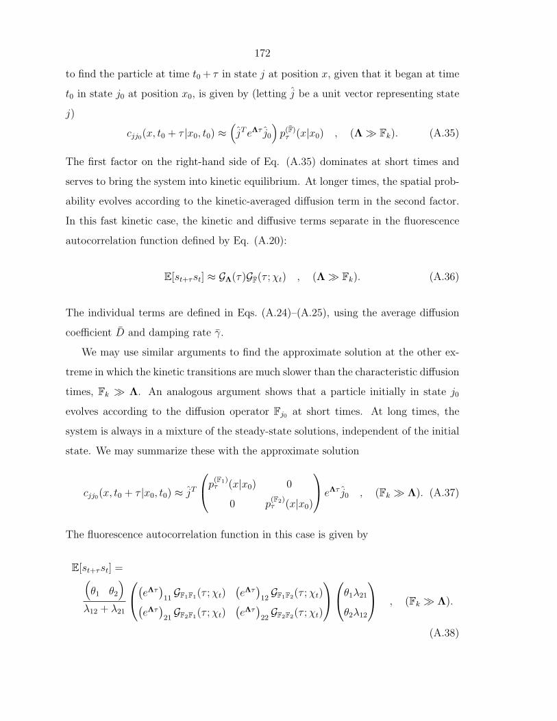
172

to find the particle at time t0 + τ in state j at position x, given that it began at time

t0 in state j0 at position x0, is given by (letting j be a unit vector representing state

j)

cjj0(x, t0 + τ |x0, t0) ≈(jT eΛτ j0

)p(F)

τ (x|x0) , (Λ Fk). (A.35)

The first factor on the right-hand side of Eq. (A.35) dominates at short times and

serves to bring the system into kinetic equilibrium. At longer times, the spatial prob-

ability evolves according to the kinetic-averaged diffusion term in the second factor.

In this fast kinetic case, the kinetic and diffusive terms separate in the fluorescence

autocorrelation function defined by Eq. (A.20):

E[st+τst] ≈ GΛ(τ)GF(τ ;χt) , (Λ Fk). (A.36)

The individual terms are defined in Eqs. (A.24)–(A.25), using the average diffusion

coefficient D and damping rate γ.

We may use similar arguments to find the approximate solution at the other ex-

treme in which the kinetic transitions are much slower than the characteristic diffusion

times, Fk Λ. An analogous argument shows that a particle initially in state j0

evolves according to the diffusion operator Fj0 at short times. At long times, the

system is always in a mixture of the steady-state solutions, independent of the initial

state. We may summarize these with the approximate solution

cjj0(x, t0 + τ |x0, t0) ≈ jT

p(F1)τ (x|x0) 0

0 p(F2)τ (x|x0)

eΛτ j0 , (Fk Λ). (A.37)

The fluorescence autocorrelation function in this case is given by

E[st+τst] =(θ1 θ2

)λ12 + λ21

(eΛτ)11GF1F1(τ ;χt)

(eΛτ)12GF1F2(τ ;χt)(

eΛτ)21GF2F1(τ ;χt)

(eΛτ)22GF2F2(τ ;χt)

θ1λ21

θ2λ12

, (Fk Λ).

(A.38)

173

The cross terms are given by

GFjFk(τ ;χt) ≡

∫∫dx2dx1Φt+τ (x2)Φt(x1)p

(Fj)τ (x2|x1)p

(Fk)0 (x2) (A.39)

with Φt(x) given by Eq. (A.21).(eΛτ)

jkis the jk entry of the matrix eΛτ . Although

they are just given by tractable Gaussian integrals, we do not need to calculate the

full expression for the cross terms GFjFk(τ ;χt) because Eq. (A.37) was derived for

the case that the kinetic transitions are much slower than the diffusion time. In that

case, the 2× 2 matrix in Eq. (A.37) is diagonal at short times, when eΛτ ≈ I, so we

need not calculate the off-diagonal cross terms. At long times, when eΛτ is no longer

diagonal, the diffusion terms have relaxed to their steady states where the cross terms

become uncorrelated:

GFjFk(τ ;χt) ≈

√ζjζk exp

[−2ζjχ

2t+τ − 2ζkχ

2t

], (Fk Λ) (A.40)

with ζj given by Eq. (A.23) with parameters taken from operator Fj.

A.4 Generalization of van Kampen’s method to

the noncommuting case

In this section, we will attempt a solution to the full, noncommuting case of Eq. (A.8)

with n = 2. We will attack the problem using the trajectory averaging approach found

in Ref. [36]. However, as mentioned earlier, van Kampen’s treatment of this problem

is equivalent to our commuting case [Fj,Fk] = 0 and we have already solved that

problem. We therefore require a generalization of that approach to this noncommuting

case.

In contrast to earlier sections, we will now expand our solution in eigenfunctions

of the two diffusion operators F1 and F2, which no longer share an eigenbasis. We will

use superscripts to indicate the basis in which a quantity is written. For example,

we may represent a function f(x) in the basis of eigenfunctions of Fk as an infinite-

174

dimensional column vector α(k) whose nth component is α(k)n :

f(x) =∞∑

n=0

α(k)n F (k)

n (x) ↔ α(k). (A.41)

We may calculate the infinite dimensional matrix V(jk) that transforms a vector from

basis k to basis j:

α(j) = V(jk)α(k) ⇐⇒ α(j)m =

∞∑n=0

V (jk)mn α(k)

n . (A.42)

The explicit form of V(jk) may be found using known properties of the Hermite

functions [37]. The nm component of this matrix is 0 wherever m > n and wherever

(m + n) is odd (note that the indexing begins at n = 0, m = 0). We will refer to

such a matrix as “Even Lower-Triangular” or ELT. The only (potentially) non-zero

entries are of the form V(jk)n+2m,n with m = 0, 1, . . . These entries are given by

V(jk)n+2m,n =

2−2m

m!

(σk

σj

)n+1(σ2

k

σ2j

− 1

)m

. (A.43)

Of course, V(kj) is the inverse of V(jk).

We may now calculate the time evolution of a state under the action of the oper-

ator Fk. Suppose the system starts in state k at time t = 0 in the spatial distribution

f(x, 0) represented by the vector α(k)(0). Then, given that no internal state transi-

tions occur, the state at time t is given by

f(x, t) =∞∑

n=0

e−nγktα(k)n (0)F (k)

n (x). (A.44)

We may represent time evolution under operator Fk, in the basis of this operator’s

eigenfunctions, by a diagonal matrix T(k)Fk

(t) whose entries are given by

[T

(k)Fk

(t)]

nn= exp (−nγkt) . (A.45)

175

Using the basis change matrices, we may also write the time evolution matrix under

operator Fk in basis j

T(j)Fk

(t) = V(jk)T(k)Fk

V(kj). (A.46)

Note that the operators T are valid only conditionally; that is, they represent time

evolution over macroscopic time intervals given that no internal state transitions occur

during the evolution. In order to construct full, unconditional solutions to Eq. (A.8),

we must average the time evolution over all possible sequences of state transitions.

Suppose that a particle starts in state 1 at time t = 0, in a spatial state specified

by α(k)(0), and that it undergoes exactly 2N transitions after time intervals ∆1, ∆′1,

∆2, ∆′2, . . . , ∆N , ∆′

N , respectively. For bookkeeping, we define the final interval

∆f = t − ∆1 − ∆′1 − · · · − ∆N − ∆′

N . We then know that the (conditional) spatial

state of the system at time t is given by

α(k)cond(t) = T

(k)F1

(∆f )T(k)F2

(∆′N)T

(k)F1

(∆N) · · ·T(k)F2

(∆′1)T

(k)F1

(∆1)α(k)(0) (A.47)

while an elementary probability argument shows that the probability density for the

sequence of transitions to occur after time intervals ∆1,∆′1, · · · ,∆N ,∆

′N ,∆f (within

the macroscopic interval [0, t]) is given by

e−λ21∆f

(λ12e

−λ12∆′N

) (λ21e

−λ21∆N)· · ·(λ12e

−λ12∆′1

) (λ21e

−λ21∆1). (A.48)

Now suppose that the particle starts in internal state 1 in a spatial state given by

α(k)(0|1). Then the unconditional probability that it is in state 1 and at position x

176

at time t is given by an average over these sequences

α(k)(1, t|1) =∞∑

N=0

∫· · ·∫d∆fd∆

′Nd∆N · · · d∆′

1d∆1

×

δ (t−∆f −∆′

N −∆N − · · · −∆′1 −∆1)

[e−λ21∆f T

(k)F1

(∆f )]

×[λ12e

−λ12∆′N T

(k)F2

(∆′N)] [λ21e

−λ21∆′N T

(k)F1

(∆N)]· · ·

×[λ12e

−λ12∆′1T

(k)F2

(∆′1)] [λ21e

−λ21∆′1T

(k)F1

(∆1)]

α(k)(0|1). (A.49)

We recognize the integrand as a matrix multiconvolution integral, which may be

written as a simple matrix product in terms of Laplace transforms. Let α(s, 1|1)

denote the Laplace transform of the state vector α(t, 1|1) with respect to t (for vector

and matrix arguments, the transform is performed element-wise) and let

Q(k)F1

(s) = λ21

∫ ∞

0

e−∆se−λ21∆T(k)F1

(∆)d∆ (A.50a)

Q(k)F2

(s) = λ12

∫ ∞

0

e−∆se−λ12∆T(k)F2

(∆)d∆. (A.50b)

Then we see immediately that

α(k)(s, 1|1) =1

λ21

Q(k)F1

(s)∞∑

N=0

[Q

(k)F2

(s)Q(k)F1

(s)]N

α(k)(0|1)

=1

λ21

Q(k)F1

(s)[I−Q

(k)F2

(s)Q(k)F1

(s)]−1

α(k)(0|1). (A.51)

Note that Q(k)Fk

(s) is diagonal with

[Q

(1)F1

(s)]

nn=

1

s+ λ21 + nγ1

(A.52)

and similarly for state 2. Furthermore, Q(k)Fj

(s) = V(kj)Q(j)Fj

(s)V(jk). Finally, note

that α(k)(s, 1|1) is the Laplace transform of the state vector representing the spatial

probability of finding the particle at position x at time t and in state 1, given that

it started in state 1 at time t = 0. Now let α(j2)(s, j2|j1) denote the corresponding

177

probability to find the particle in state j2 at time t given that it began in internal

state j1 and spatial state α(j1)(0|j1), and let R(j2j1)j2j1

(s) be the operator relating these

vectors:

α(j2)(s, j2|j1) = R(j2j1)j2j1

(s)α(j1)(0|j1). (A.53)

Note that we have written the components of the initial and final states in their

natural bases (i.e. the j1 component of the initial state is written in basis j1). There

are four allowable pairs of values for j1 and j2, and analogous arguments to those

given above show that the probability densities for each case are given by

R(11)11 (s) =

1

λ21

Q(1)F1

(s)[I−Q

(1)F2

(s)Q(1)F1

(s)]−1

(A.54a)

R(21)21 (s) =

1

λ12

V(21)Q(1)F2

(s)[I−Q

(1)F1

(s)Q(1)F2

(s)]−1

Q(1)F1

(s) (A.54b)

R(12)12 (s) =

1

λ21

V(12)Q(2)F1

(s)[I−Q

(2)F2

(s)Q(2)F1

(s)]−1

Q(2)F2

(s) (A.54c)

R(22)22 (s) =

1

λ12

Q(2)F2

(s)[I−Q

(2)F1

(s)Q(2)F2

(s)]−1

. (A.54d)

Let us summarize these results using the following notation. Suppose that the

system starts in the state

c(x, 0) =∞∑

n=0

α(1)n (0)F

(1)n (x)

β(2)n (0)F

(2)n (x)

↔

α(1)(0)

β(2)(0)

(A.55)

where the vector on the right is doubly infinite, and should only be thought of as a

shorthand notation for writing both (infinite) vectors. Denoting the solution at time

t by

c(x, t) =∞∑

n=0

α(1)n (t)F

(1)n (x)

β(2)n (t)F

(2)n (x)

↔

α(1)(t)

β(2)(t)

, (A.56)

we may summarize the full solution computed above byα(1)(t)

β(2)(t)

=

R(11)11 (t) R

(12)12 (t)

R(21)21 (t) R

(22)22 (t)

α(1)(0)

β(2)(0)

. (A.57)

178

In principle, at least, we have given an explicit solution to the full noncommuting

problem to an arbitrary order in terms of its Laplace transform. Although Eqs.

(A.54a-A.54b) represent infinite-dimensional matrix multiplication and inversion, we

may still make a bit more analytical progress in many cases. It is straightforward

to show that products and inverses of ELT matrices are themselves ELT matrices,

so that R(j1j2)j1j2

(s) is an ELT matrix. Furthermore, ELT matrix inverses have the

special property that the upper-left N ×N block of the inverse of an ELT matrix is

exactly the inverse of the upper-left N × N block. A similar relation holds for ELT

matrix sums and products. Therefore, we may calculate finite-order matrix elements

of R(j1j2)j1j2

(s) by manipulating truncations of Q(k)Fj

(s) at the same order. In other words,

if the system begins in a state that can be approximated by a finite truncation of

the eigenfunction expansion, then its time evolution will remain inside that truncated

subsystem. As a result of this nice subsystem decoupling, in principle at least, we can

explicitly calculate the matrix elements of R(j1j2)j1j2

(s) to any order. In practice this is

quite cumbersome, of course.

179

References

[1] A. J. Berglund, A. C. Doherty, and H. Mabuchi. Photon statistics and dynamics

of Fluorescence Resonance Energy Transfer. Phys. Rev. Lett., 89:068101, 2002.

[2] A. J. Berglund and H. Mabuchi. Feedback controller design for tracking a single

fluorescent molecule. Appl. Phys. B, 78:653–659, 2004.

[3] K. McHale, A. J. Berglund, and H. Mabuchi. Bayesian estimation for species

identification in single-molecule fluorescence microscopy. Biophys. J., 86:3409–

3422, 2004.

[4] A. J. Berglund. Nonexponential statistics of fluorescence photobleaching. J.

Chem. Phys., 121:2899–2903, 2004.

[5] S. Weiss. Fluorescence spectroscopy of single biomolecules. Science, 283:1676–

1683, 1999.

[6] D. Magde, E. L. Elson, and W. W. Webb. Thermodynamic fluctuations in a

reacting system - measurement by fluorescence correlation spectroscopy. Phys.

Rev. Lett., 29:705–708, 1972.

[7] E. L. Elson and D. Magde. Fluorescence correlation spectroscopy. 1. Conceptual

basis and theory. Biopolymers, 13:1–27, 1974.

[8] D. Magde, E. L. Elson, and W. W. Webb. Fluorescence correlation spectroscopy.

2. Experimental realization. Biopolymers, 13:29–61, 1974.

[9] O. Krichevsky and G. Bonnett. Fluorescence correlation spectroscopy: The

technique and its applications. Rep. Prog. Phys., 65:251–297, 2002.

180

[10] H. C. Berg. How to track bacteria. Rev. Sci. Instr., 42:868–871, 1971.

[11] T. Ha, D. S. Chemla, Th. Enderle, and S. Weiss. Single molecule spectroscopy

with automated positioning. Appl. Phys. Lett., 70:782–784, 1997.

[12] J. Enderlein. Tracking of fluorescent molecules diffusing within membranes. Appl.

Phys. B, 71:773–777, 2000.

[13] J. Enderlein. Positional and temporal accuracy of single molecule tracking. Sing.

Mol., 1:225–230, 2000.

[14] S. B. Andersson. Tracking a single fluorescent molecule in a confocal microscope.

Appl. Phys. B, 80:809–816, 2005.

[15] R. S. Decca, C.-W. Lee, and S. R. Wassall. Single molecule tracking scheme

using a near-field scanning optical microscope. Rev. Sci. Instr., 73:2675–2679,

2002.

[16] V. Levi, Q. Ruan, K. Kis-Petikova, and E. Gratton. Scanning FCS, a novel

method for three-dimensional particle tracking. Biochem. Soc. Trans., 31:997–

1000, 2003.

[17] K. Kis-Petikova and E. Gratton. Distance measurement by circular scanning of

the excitation beam in a two-photon microscope. Microsc. Res. Tech., 63:34–49,

2004.

[18] V. Levi, V. Ruan, and E. Gratton. 3-D particle tracking in a two-photon mi-

croscope. Application to the study of molecular dynamics in cells. Biophys. J.,

88:2919–2928, 2005.

[19] V. Levi, V. Ruan, Matthew Plutz, A. S. Belmont, and E. Gratton. Chromatin

Dynamics in Interphase Cells Revealed by Tracking in a Two-Photon Excitation

Microscope. Biophys. J., 89:4275–4285, 2005.

181

[20] H. Cang, C. M. Wong, C. S. Xu, A. H. Rizvi, and H. Yang. Confocal three dimen-

sional tracking of a single nanoparticle with concurrent spectroscopic readout.

Appl. Phys. Lett., 88:223901, 2006.

[21] D. Montiel, H. Cang, and H. Yang. Quantitative characterization of changes in

dynamical behavior for single-particle tracking studies. To appear in J. Phys.

Chem. B, 2006.

[22] A. E. Cohen and W. E. Moerner. Method for trapping and manipulating

nanoscale objects in solution. Appl. Phys. Lett., 86:093109, 2005.

[23] A. E. Cohen. Control of nanoparticles with arbitrary two-dimensional force fields.

Phys. Rev. Lett., 94:118102, 2005.

[24] A. E. Cohen and W. E. Moerner. Suppressing Brownian motion of individual

biomolecules in solution. Proc. Natl. Acad. Sci. USA, 103:4362–4365, 2006.

[25] A. J. Berglund and H. Mabuchi. Tracking-FCS: Fluorescence Correlation Spec-

troscopy of individual particles. Opt. Express, 13:8069–8082, 2005.

[26] A. J. Berglund and H. Mabuchi. Performance bounds on single-particle tracking

by fluorescence modulation. Appl. Phys. B, 83:127–133, 2006.

[27] A. J. Berglund, K. McHale, and H. Mabuchi. Feedback localization of freely

diffusing fluorescent particles near the optical shot-noise limit. To appear in

Opt. Lett., 2006.

[28] A. J. Berglund, K. McHale, and H. Mabuchi. Fast classification of freely-diffusing

fluorescent nanoparticles. In preparation, 2006.

[29] K. McHale, A. J. Berglund, and H. Mabuchi. Near-optimal dilute concentration

estimation via single-molecule detection. In preparation, 2006.

[30] O. L. R. Jacobs. Introduction to Control Theory. Oxford University Press, New

York, 2nd edition, 1996.

182

[31] C. W. Gardiner. Handook of Stochastic Methods for Physics, Chemistry and the

Natural Sciences. Springer-Verlag, New York, 2nd edition, 1985.

[32] R. S. Lipster and A. N. Shiryaev. Statistics of Random Processes I. Springer,

New York, 2001.

[33] P. E. Kloeden, E. Platen, and H. Shurz. Numerical Solution of SDE Through

Computer Experiments. Springer, New York, 1997.

[34] K. Zhou, J. C. Doyle, and K. Glover. Robust and Optimal Control. Prentice

Hall, 1996.

[35] J. Doyle, B. Francis, and A. Tannenbaum. Feedback Control Theory. Macmillan

Publishing Co., 1990.

[36] N. G. Van Kampen. Stochastic processes in physics and chemistry. Elsevier

Science Pub. Co., North-Holland, Amsterdam, 2001.

[37] I. S. Gradshteyn and I. M. Ryzhik. Table of Integrals, Series and Products.

Academic press, San Diego, 6th edition, 1980.

[38] C. W. Gardiner and A. Eschmann. Master-equation theory of semiconductor

lasers. Phys. Rev. A, 51:4982–4995, 1995.

[39] A. Yildiz, J. N. Forkey, S. A. McKinney, T. Ha, Y. E. Goodman, and Paul R.

Selvin. Myosin V walks hand-over-hand: Single fluorophore imaging with 1.5-nm

localization. Science, 300:2061–2065, 2003.

[40] H. Risken. The Fokker-Planck Equation: Methods of Solution and Applications.

Springer, 2nd edition, 1989.

[41] S. Saffarian and E. L. Elson. Statistical analysis of Fluorescence Correlation

Spectroscopy: The standard deviation and bias. Biophys. J., 84:2030–2042,

2003.

183

[42] T. Meyer and H. Schindler. Simultaneous measurement of aggregation and dif-

fusion of molecules in solutions and in membranes. Biophys. J., 54:983–993,

1988.

[43] M. A. Digman, C. M. Brown, P. Sengupta, P. W. Wiseman, A. R. Horwitz, and

E. Gratton. Measuring fast dynamics in solutions and cells with a laser scanning

microscope. Biophys. J., 90:1317–1327, 2005.

[44] L. L. Smith and P. M. Koch. Use of four mirrors to rotate linear polarization

but preserve input-output collinearity. J. Opt. Soc. Am. A, 13:2102–2105, 1996.

[45] E. J. Galvez and P. M. Koch. Use of four mirrors to rotate linear polarization but

preserve input-output collinearity. ii. J. Opt. Soc. Am. A, 14:3410–3414, 1997.

[46] E. Wolf. Electromagnetic diffraction in optical systems. I. An integral represen-

tation of the image field. Proc. Roy. Soc. London, 253:349–357, 1959.

[47] M. Mansuripur. Distribution of light at and near the focus of high-numerical-

aperture objectives. J. Opt. Soc. Am. A, 3:2086–2094, 1986.

[48] M. Mansuripur. Certain computational aspects of vector diffraction problems.

J. Opt. Soc. Am. A, 6:786–805, 1989.

[49] M. Mansuripur. Effects of high-numerical-aperture focusing on the state of polar-

ization in optical and magneto-optic data storage systems. Appl. Opt., 30:3154–

3162, 1991.

[50] L. Novotny, R. D. Grover, and K. Karrai. Reflected image of a strongly focused

spot. Opt. Lett., 26:789–791, 2001.

[51] M. Doi and S. F. Edwards. The Theory of Polymer Dynamics. Oxford University

Press, Oxford, 1986.

[52] A. Gennerich and D. Schild. Fluorescence correlation spectroscopy in small cy-

tosolic compartments depends critically on the diffusion model used. Biophys.

J., 79:3294–3306, 2000.

184

[53] L. P. Faucheux and A. J. Libchaber. Confined Brownian motion. Phys. Rev. E,

49:5158–5163, 1994.

[54] B. Lin, J. Yu, and S. A. Rice. Direct measurements of constrained Brownian

motion of an isolated sphere between two walls. Phys. Rev. E, 62:3909–3919,

2000.

[55] K. Schatzel, M. Drewel, and S. Stimac. Photon correlation measurements at

large lag times: Improving statistical accuracy. J. Mod. Opt., 35:711–718, 1988.

[56] T. A. Laurence, S. Fore, and T. Huser. Fast, flexible algorithm for calculating

photon correlations. Opt. Lett., 31:829–831, 2006.

[57] G. Chirico, C. Fumagalli, and G. Baldini. Trapped Brownian motion in single-

and two-photon excitation fluorescence correlation experiments. J. Phys. Chem.

B, 106:2508–2519, 2002.

[58] M. H. DeGroot. Probability and Statistics. Addison-Wesley, Reading, MA, 1986.

[59] M. Abramowitz and I. Stegun, editors. Handbook of Mathematical Functions,

with Formulas, Graphs, and Mathematical Tables. Dover Publications, New York,

9th edition, 1972.

[60] Y. Chen, J. D. Muller, V. Ruan, and E. Gratton. Molecular brightness charac-

terization of EGFP in vivo by fluorescence fluctuation spectroscopy. Biophys. J.,

82:133 – 1414, 2002.

[61] E. Rhoades, E. Gussakovsky, and G. Haran. Watching proteins fold one molecule

at a time. Proc. Natl. Acad. Sci. USA, 100:3197–3202, 2003.

[62] D. E. Koppel, M. P. Sheetz, and M. Schindler. Matrix control of protein diffusion

in biological membranes. Proc. Natl. Acad. Sci. USA, 78:3576–3580, 1981.

[63] H. Qian. Equations for stochastic macromolecular mechanics of single proteins:

Equilibrium fluctuations, transient kinetics and nonequilibrium steady-state. J.

Phys. Chem. B, 106:2065–2073, 2002.

185

[64] W. Magnus, F. Oberhettinger, and R. P. Soni. Formulas and Theorems for the

Special Functions of Mathematical Physics. Springer-Verlag, New York, 1966.

Feedback Control of Brownian Motion for Single-Particle ...

Documents

Transcript of Feedback Control of Brownian Motion for Single-Particle ...