Feature Tracking with Automatic selection of spatial - DiVA Portal

Feature Tracking with Automatic Selection of

Spatial Scales

Lars Bretzner and Tony Lindeberg

Computational Vision and Active Perception Laboratory (CVAP),

Department of Numerical Analysis and Computing Science,

KTH, S-100 44 Stockholm, Sweden.

Email: bretzner@@bion.kth.se, tony@@bion.kth.se

Technical report ISRN KTH NA/P{96/21{SE.

Abstract

When observing a dynamic world, the size of image structures may varyover time. This article emphasizes the need for including explicit mecha-nisms for automatic scale selection in feature tracking algorithms in orderto: (i) adapt the local scale of processing to the local image structure, and(ii) adapt to the size variations that may occur over time.

The problems of corner detection and blob detection are treated in de-tail, and a combined framework for feature tracking is presented in whichthe image features at every time moment are detected at locally deter-mined and automatically selected scales. A useful property of the scaleselection method is that the scale levels selected in the feature detectionstep re ect the spatial extent of the image structures. Thereby, the in-tegrated tracking algorithm has the ability to adapt to spatial as well astemporal size variations, and can in this way overcome some of the inherentlimitations of exposing �xed-scale tracking methods to image sequences inwhich the size variations are large.

In the composed tracking procedure, the scale information is used fortwo additional major purposes: (i) for de�ning local regions of interest forsearching for matching candidates as well as setting the window size forcorrelation when evaluating matching candidates, and (ii) stability overtime of the scale and signi�cance descriptors produced by the scale selec-tion procedure are used for formulating a multi-cue similarity measure formatching.

Experiments on real-world sequences are presented showing the perfor-mance of the algorithm when applied to (individual) tracking of cornersand blobs. Speci�cally, comparisons with �xed-scale tracking methods areincluded as well as illustrations of the increase in performance obtainedby using multiple cues in the feature matching step.

Keywords: feature, tracking, motion, blob, corner, scale, scale-space, scaleselection, similarity, computer vision

i

ii Bretzner and Lindeberg

Contents

1 Introduction 1

2 The need for automatic scale selection in feature tracking 3

3 Feature detection with automatic scale selection 4

3.1 Normalized derivatives . . . . . . . . . . . . . . . . . . . . . 4

3.2 Corner detection with automatic scale selection . . . . . . . 5

3.3 Blob detection with automatic scale selection . . . . . . . . 5

4 Tracking and prediction in a multi-scale context 6

5 Matching on multi-cue similarity 7

6 Combined tracking algorithm 8

7 Experimental results 10

7.1 Corner tracking . . . . . . . . . . . . . . . . . . . . . . . . . 10

7.2 Blob tracking . . . . . . . . . . . . . . . . . . . . . . . . . . 12

8 Summary and Discussion 14

8.1 Spatial consistency and statistical evaluation. . . . . . . . . 15

8.2 Multi-cue tracking . . . . . . . . . . . . . . . . . . . . . . . 15

8.3 Temporal consistency . . . . . . . . . . . . . . . . . . . . . 16

A Algorithmic details 20

A.1 Prediction . . . . . . . . . . . . . . . . . . . . . . . . . . . . 20

A.2 Feature detection . . . . . . . . . . . . . . . . . . . . . . . . 20

A.3 Matching . . . . . . . . . . . . . . . . . . . . . . . . . . . . 20

Feature Tracking with Automatic Selection of Spatial Scales 1

1 Introduction

Being able to track image structures over time is a useful and sometimes nec-essary capability for vision systems intended to interact with a dynamic world.There are several computer vision algorithms in which tracking arises as animportant subproblem. Some situations are:

� Fixation means maintaining a relationship between a physical point orregion in the world and some (usually central) region in a camera system.To maintain such a relationship over time, we have to relate some char-acteristic properties of the physical point to entities that are measurablefrom the available image data.

� Object recognition in a dynamically varying environment gives rise to thesame type of problem, including the case when the visual agent is activeand moves relative to the scene. Examples of the latter are navigationas well as active scene exploration. When objects move relative to theobserver, feature tracking is a useful processing step for preserving theidentity of image features over time.

� The identity problem is also essential in algorithms for motion segmen-tation and structure from motion. To compute structural properties orinvariant descriptors which depend on the temporal variation of a geomet-ric con�guration, some mechanism is needed for matching correspondingimage features over time.

There is an extensive literature on tracking methods operating without speci�ca priori knowledge about the world, such as object models or highly restricteddomains. Without any aim of giving an extensive survey, the work in this di-rection can be classi�ed into three main categories:

Correlation based tracking The presumably earliest approach to image match-ing is the correlation technique based on the similarity between correspondinggrey-level patches over time. Given a window of some size, which covers an im-age detail at a certain time moment, the corresponding detail at the next timemoment is de�ned as the position of the window (of the same size) that givesthe highest correlation score when compared to the previous patch.

Optical ow based tracking The de�nition of an optic ow �eld gives rise toa motion �eld in the image domain, which can be interpreted as the result oftracking all image points simultaneously. With respect to the tracking problem,the motion of coherently moving (and possibly segmented) regions computedfrom optic ow algorithms can be used for guiding tracking procedures, asshown by [Thompson et al., 1993] and [Meyer and Bouthemy, 1994].

Feature tracking Over the years a large number of approaches have been devel-oped for tracking image features such as edges and corners over time. Essentially,what characterizes a feature tracking method is that image features are �rst ex-tracted in a bottom-up processing step and then these features are used as the

2 Bretzner and Lindeberg

main primitives for the tracking and matching procedures. Concerning cornertracking, [Shapiro et al., 1992b] detect and track corners individually in an al-gorithm originally aimed at applications such as videoconferencing. [Smith andBrady, 1995] track a large set of corners and use the results in a ow-based seg-mentation algorithm. [Zheng and Chellappa, 1995] have studied feature trackingwhen compensating for camera motion, and [Gee and Cipolla, 1995] track lo-cally darkest points with applications to pose estimation. In contour tracking,[Blake et al., 1993, Curwen et al., 1991] use snakes to track moving, deformingimage features. [Cipolla and Blake, 1992] apply such an approach to estimatetime-to-contact, and [Koller et al., 1994] track combined motion and grey-levelboundaries in traÆc surveillance. An overview of di�erent approaches to edgetracking can be found in the recent book by [Faugeras, 1993].

The subject of this article is to consider the domain of feature tracking andto complement previous works on this subject by addressing the problem ofscale and scale selection in the spatial domain and by introducing new simi-larity measures in the matching step. In most previous works, the analysis isperformed at a single predetermined scale. Here, we will emphasize and showby examples why it is useful to include an explicit mechanism for automaticscale selection to be able to handle situations in which the size variations arelarge. Besides avoiding explicit setting of scale levels for feature detection, andthus overcoming some of the fundamental limitations of processing image se-quences at a single scale, it will be demonstrated how scale levels selected bya scale selection procedure can constitute a useful source of information whende�ning a similarity measure over time, as well as for adapting the window sizefor correlation to the local image structure.

Moreover, since the resulting matching algorithm we will arrive at is basedon a similarity measure de�ned as the combination of di�erent discriminativeproperties, and with small modi�cations can be applied to tracking of bothcorners and blobs, we will emphasize this multi-cue aspect as an importantcomponent for increasing the robustness of feature tracking algorithms.

The presentation is organized as follows: Section 2 illustrates the need foradaptive scale selection in feature tracking. It gives a hands-on demonstrationof the improvement in performance that can be obtained by including a scaleselection mechanism when tracking features in image sequences in which the sizevariations over time are large. Section 3 describes the feature detection step andreviews the basic components in a general principle for scale selection. Sections4 and 5 explain how the scale information obtained from these processingmodules can be used in the prediction step and in the evaluation of matchingcandidates. Section 6 summarizes how these components can be combined witha classical feature tracking scheme with prediction followed by detection andmatching. Section 7 shows the performance of the algorithm when applied toreal-world data. Feature tracking using adaptive scales is compared to trackingat one, �xed scale. Comparisons are also made between single-cue and multi-cue similarity measures. Finally, we conclude in section 8 by summarizing themain properties of the method and by outlining natural extensions.


2 The need for automatic scale selection in feature tracking

To extract features from an image, we have to apply some operators to thedata. The type of features that can be extracted are largely determined bythe spatial extent of these operators. When dealing with real-world data aboutwhich no or very little information is available, we can hardly expect to knowin advance what scales are relevant for processing a given image. Therefore, areasonable approach is to consider a large number of scales simultaneously, andthis is one of the major motivations for using a multi-scale representation whenautomatically processing measurement data such as images.

Despite this now rather well-spread insight, most work on feature track-ing still performs the analysis at one scale only. For correlation based trackingmethods, this corresponds to using a �xed-size window over time, and concern-ing feature tracking to detecting image features at the same scale at all timemoments. Such an approach will, however, su�er from inherent limitations whenapplied to real-life image sequences in which the size variations are large. Thisbasic property constitutes one illustration of why a mechanism for automaticscale selection is an essential complement to traditional multi-scale processingin general, and to feature detection and feature tracking in particular.

In an image sequence, the size of image structures may change over timedue to expansions or contractions. A typical example of the former is when theobserver approaches an object as shown in �gure 1. The left column in this�gure shows a few snapshots from a tracker which follows a corner on the objectover time using a standard feature tracking technique with a �xed scale for cor-ner detection and a �xed window size for hypothesis evaluation by correlation.After a number of frames, the algorithm fails to detect the right feature andthe corner is lost. The reason why this occurs, is simply the fact that the cornerno longer exists at the predetermined scale. As a comparison, the right columnshows the result of incorporating a mechanism for adaptation of the scale levelsto the local image structure (details will be given in later sections). As can beseen, the corner is correctly tracked over the whole sequence. (The same initialscale was used in both experiments.)

Another motivation to this work originates from the fact that all feature de-tectors su�er from localization errors due to e.g noise and motion blur. Whendetecting rigid body motion or recovering 3D structure from feature point cor-respondences in an image sequence, it is important that the motion in the sceneis large compared to the localization errors of the feature detector. If the inter-frame motion is small, we therefore have to track features over a large numberof frames to obtain accurate results. This requirement constitutes a key motiva-tion for including a scale selection mechanism in the feature tracker, to obtainlonger trajectories of corresponding features as input to algorithms for motionestimation and recovery of 3D structure.

Concerning the common use of �xed scale levels in tracking methods, it isworth pointing out that in situations where the image features are distinct (e.g.sharp corners on a smooth background), traditional methods using �xed scalesmight be suÆcient. The main advantages of having a mechanism for automatic


scale selection in such situations are that: (i) the actual tuning of the scaleparameter can be avoided, (ii) as will be illustrated later, stability over timeof the selected scale levels turns out to be a useful discriminative constraint toinclude in a matching criterion.

3 Feature detection with automatic scale selection

A natural framework to use when extracting features from image data is tode�ne the image features from multi-scale di�erential invariants expressed interms of Gaussian derivative operators [Koenderink and van Doorn, 1992, Flo-rack et al., 1992], or more speci�cally, as maxima or zero-crossings of suchentities [Lindeberg, 1994c]. In this way, image features such as corners, blobs,edges and ridges can be computed at any level of scale.

A basic problem that arises for any such feature detector concerns how todetermine at what scales the image features should be extracted, or if the featuredetection is performed at several scales simultaneously, what image featuresshould be regarded as signi�cant. A framework addressing this problem hasbeen developed in [Lindeberg, 1993, Lindeberg, 1994c]. In summary, one of themain results from this work is a general principle for scale selection, which statesthat scale levels for feature detection can be selected from the scales at whichnormalized di�erential invariants assume maxima over scales. In this section,we shall give a brief review of how this methodology applies to the detectionof features such as blobs and corners. The image features so obtained, withtheir associated attributes resulting from the scale selection method, will thenbe used as basic primitives for the tracking procedure.

3.1 Normalized derivatives

The scale-space representation [Witkin, 1983, Koenderink, 1984] of a signal fis de�ned as the result of convolving f

L(:; t) = g(:; t) � f (1)

with Gaussian kernels having di�erent values of the scale parameter t

g(x; t) =1

2�te�(x

2+y2)=(2t) (2)

In this representation, -normalized derivatives [Lindeberg, 1996a] are de�nedby

@� = t =2 @x (3)

where t is the variance of the Gaussian kernel. From this construction, a normal-ized di�erential invariant is then obtained by replacing all spatial derivativesby corresponding normalized derivatives according to (3).


3.2 Corner detection with automatic scale selection

A common way to de�ne a corner in a grey-level image in di�erential geometricterms is as a point at which both the curvature of a level curve

� =� �LyyL

2x + LxxL

2y � 2LxLyLxy

��L2x + L2

y

�3=2 (4)

and the gradient magnitude

jrLj =qL2x + L2

y (5)

are high [Kitchen and Rosenfeld, 1982, Koenderink and Richards, 1988, Dericheand Giraudon, 1990, Blom, 1992]. If we consider the product of � and thegradient magnitude raised to some power, and choose the power equal to three,we obtain the essentially aÆne invariant expression

~� = LyyL2x + LxxL

2y � 2LxLyLxy (6)

with its corresponding -normalized di�erential invariant

~� �norm = t2 ~� (7)

In [Lindeberg, 1994a] it is shown how a junction detector with automatic scaleselection can be formulated in terms of the detection of scale-space maxima of~�2 �norm, i.e., by detecting points in scale-space where ~�2 �norm assumes max-ima with respect to both scale and space. When detecting image features atcoarse scales it turns out that the localization can be poor. Therefore, this de-tection step is complemented by a second localization stage, in which a modi�edF�orstner operator [F�orstner and G�ulch, 1987], is used for iteratively computingnew localization estimates using scale information from the initial detectionstep (see the references for details).

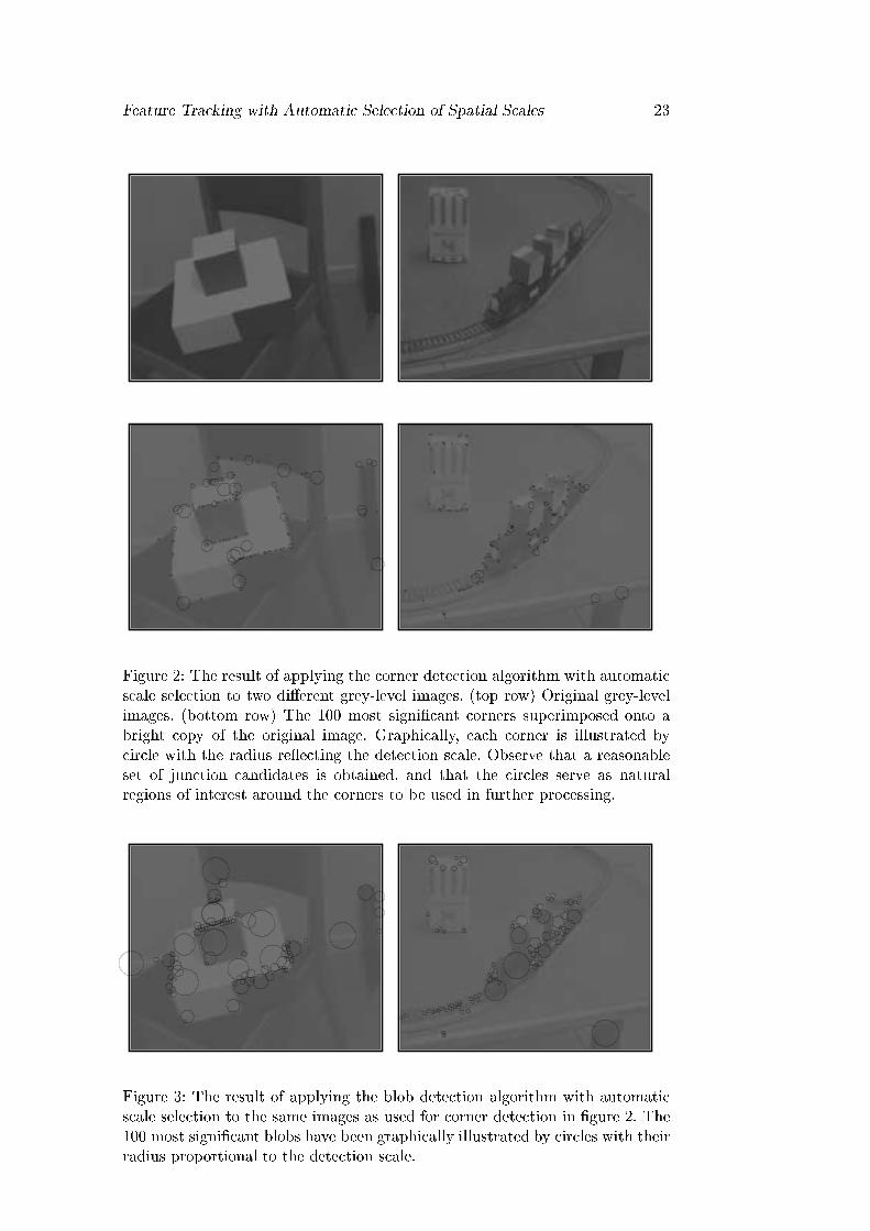
A useful property of this corner detection method is that it leads to selectionof coarser scales for corners having large spatial extent. Figure 2 illustrates thisproperty by showing the result of applying the corner detection method totwo di�erent images, and graphically illustrating each detected and localizedcorner by a circle with the radius proportional to the detection scale. Notably,the support regions of these blobs serve as natural regions of interest aroundthe detected corners. As we shall demonstrate later, such regions of interestand context information turn out to be highly useful for a feature trackingprocedure.

3.3 Blob detection with automatic scale selection

As shown in the abovementioned references, a straightforward method for blobdetection can be formulated in an analogous manner by detecting scale-spacemaxima of the square of the normalized Laplacian

r2normL = t (Lxx + Lyy) (8)


This operator gives a strong response for blobs that are brighter or darker thantheir background, and in analogy with the corner detection method, the selectedscale levels provide information about the characteristic size of the blob.

Figure 3 shows the result of applying this blob detection method to the sameimages as used in �gure 2. As can be seen, a representative set of blob featuresat di�erent scales is extracted. Moreover, it can be noted how well the blobcircles re ect the size variations, in particular, considering how simple opera-tions the blob detection algorithm is based on (Gaussian smoothing, derivativecomputation, and detection of scale-space maxima).

4 Tracking and prediction in a multi-scale context

When tracking features over time, both the position of the feature and theappearance of its surrounding grey-level pattern can be expected to change.To relate features over time, we shall throughout this work make use of thecommon assumption about small motions between successive frames.

There are several ways to predict the position of a feature in the next framebased on its positions in previous frames. Whereas the Kalman �ltering method-ology has been commonly used in the computer vision literature, this approachsu�ers from a fundamental limitation if the motion direction suddenly changes.If a feature moving in a certain direction has been tracked over a long periodof time, then the built-in temporal smoothing of the feature trajectory in theKalman �lter, implies that the predictions will continue to be in essentially thesame direction, although the actual direction of the motion changes. If the co-variance matrices in the Kalman �lter have been adapted to small oscillationsaround the previously smooth trajectory, it will hence be likely that the featureis lost at the discontinuity.1

For this reason, we shall make use of simpler �rst-order prediction, whichuses the motion between the previous two successive frames as a prediction tothe next frame.2

Within a neighbourhood of each predicted feature position, we detect newfeatures using the corner (or blob) detection procedure with automatic scaleselection. The support regions associated with the features serve as naturalregions of interest when searching for new corresponding features in the nextframe. In this way, we can avoid the problem of setting a global thresholdon the distance between matching candidates. There is, of course, a certainscaling factor between the detection scale and the size of the support region.The important property of this method, however, is that it will automaticallyselect smaller regions of interest for small-size image structures, and largersearch regions for larger size structures. Here, we shall make use of this scaleinformation for three main purposes:

1As will be shown in the experiments in section 7, the resulting feature trajectories may be

quite irregular. Enforced temporal smoothing of the image positions of the features, leading

to smoother trajectories, would not be appropriate for such data.2Both constant acceleration and constant velocity models have been used, but the latter

has given better performance in most cases.


� Setting the search region for possible matching candidates.

� Setting the window size for correlation matching.

� Using the stability of the detection scale as a matching condition.

We set the size of the search region to the spatial extent of the previous imagefeature, multiplied by a safety factor. Within this window, a certain number ofcandidate matches are selected. Then, an evaluation of these matching candi-dates is made based on a combined similarity measure to be de�ned in the nextsection.

5 Matching on multi-cue similarity

Based on the assumption of small inter-frame image motions, we use a multi-ple cue approach to the feature matching problem. Instead of evaluating thematching candidates using a correlation measure on a local grey-level patchonly, as done in most feature tracking algorithms, we combine the correlationmeasure with signi�cance stability, scale stability and proximity measures asde�ned below.

Patch similarity. This measure is a normalized Gaussian-weighted intensitycross-correlation between two image patches. Here, we compute this measureover a square centered at the feature and with its size set from the detectionscale. The measure is derived from the cross-correlation of the image patches,see [Shapiro et al., 1992a], computed using a Gaussian weight function centeredat the feature. The motivation for using a Gaussian weight function is thatimage structures near the feature center should be regarded as more signi�cantthan peripheral structures. Given two brightness functions IA and IB, and twoimage regions DA � R and DB � R of the same size jDj = jDAj = jDB jcentered at pA and pB respectively, the weighted cross-correlation between thepatches is de�ned as:

C(A;B) =1

jDjXx2DA

e�(x�pA)2

IA(x) IB(x� pA + pB)�

1

jDj2X

xA2DA

e�(x�pA)2

IA(xA)X

xB2DB

e�(x�pB)2

IB(xB) (9)

and the normalized weighted cross-correlation is

Spatch(A;B) =C(A;B)p

C(A;A)C(B;B)(10)

where

C(A;A) =1

jDjXx2DA

(e�(x�pA)2

IA(x))2 � 1

jDj2 (Xx2DA

e�(x�pA)2

IA(x))2

(11)

and C(B;B) is de�ned analogously. As is well-known, this similarity measureis invariant to superimposed linear illumination gradients. Hence, �rst-ordere�ects of scene lightning do not a�ect this measure, and the measure onlyaccounts for changes in the structure of the patches.


Signi�cance stability. A straightforward signi�cance measure of a feature de-tected according to the method described in section 3 is the normalized responseat the local scale-space maximum. For corners, this measure is the normalizedlevel curve curvature according to (7) and for blobs it is the normalized Lapla-cian according to (8). To compare signi�cance values over time, we measuresimilarity by relative di�erences instead of absolute, and de�ne this measure as

Ssign = j log RB

RAj (12)

where RA and RB are the signi�cance measures of the corresponding featuresA and B.

Scale stability. Since the features are detected at di�erent scales, the ratiobetween the detection scales of two features constitutes a measure of stabilityover scales. To measure relative scale variations, we use the absolute value ofthe logarithm of this ratio, de�ned as

Sscale = j log tBtAj (13)

where tA and tB are the detection scales of A and B.

Proximity We measure how well the position xA of feature A corresponds tothe position xpred predicted from feature B

Spos =kxA � xpredkp

tB(14)

where tB is the detection scale feature B.

Combined similarity measure. In summary, the similarity measure we makeuse of a weighted sum of (10), (12) and (13),

Scomb = cpatchSpatch + csignSsign + cscaleSscale + cposSpos (15)

where cpatch, csing, cscale and cpos are tuning parameters to be determined.

6 Combined tracking algorithm

By combining the components described in the previous sections, we obtain afeature tracking scheme based on a traditional predict-detect-update loop. Inaddition, the following processing steps are added:

� Quality measure. Each feature is assigned a quality measure indicatinghow stable it is over time.

� Bidirectional matching. To provide additional information to later pro-cessing stages about the reliability of the matches, the matching can bedone bidirectionally. Given a feature F1 from the feature set, we �rst com-pute its winning matching candidate F2 in the current image. If then F1


is the winning candidate of F2 in the backward matching direction, thematch between F1 and F2 is registered as safe. This processing step isuseful for signalling possible matching errors.

During the tracking procedure each feature is associated with the followingattributes:

{ its detection scale tdet,

{ its estimated size D = ksize �ptdet bounded from below to Dmin,

{ its position,

{ its quality value.

An overview of the tracking algorithm is given in �gure 4. At a more detailedlevel, each individual module operates as follows:

Prediction The prediction is performed as described in section 4. For eachfeature in the feature set, a linear prediction of the position in the currentframe is computed based on the positions of the corresponding feature in thetwo previous frames. The size of the search window is computed as kw1 � D(with the size D bounded from below). When a trajectory is initiated, there isno feature history to base the prediction on, so we use a larger search window ofsize kw2 �D (kw2 > kw1) and use the original feature position as the predictedposition.

Detection In each frame, image features are detected as described in section 3.The window obtained from the prediction step is searched for the same kind offeatures over a locally adapted range of scales [tmin; tmax], where tmax = krange�tdet and tmin = tdet=krange. The number n of detected candidates depends onwhich feature extraction method we use in the detection step.

Matching The matching is based on the similarity measures described in sec-tion 5. The original feature is matched to the candidates obtained from thedetection step and the winner is the feature having the highest combined simi-larity value above a �xed threshold Tcomb and a patch correlation value above athreshold Tpatch. These thresholds are necessary to suppress false matches whenfeatures disappear due to e.g occlusion.

If a feature is matched, the quality value is increased by dqi and its position,its scale descriptor, its signi�cance value and its grey-level patch are updated.

If no match is found, the feature is considered unmatched, its quality valueis decreased by dqd and its position is set to the predicted position.

Finally for each frame, the feature set is parsed to detect feature merges andto remove features having quality values below a threshold Tq. When two fea-tures merge, their trajectories are terminated and a new trajectory is initiated.In this way, we obtain more reliable feature trajectories for further processing.


7 Experimental results

7.1 Corner tracking

Let us �rst demonstrate the performance of the algorithm when applied to animage sequence consisting of 60 frames. In this sequence, the camera moves ina fairly complex way relative to a static scene. The objects of interest on whichthe features (here corners) are detected are a telephone and a package on atable. From the junctions detected in the initial frame, a subset of 14 featureswere selected manually as shown in �gure 5.

Figure 6 shows the situation after 30, 50 and 60 frames. In the illustrations,black segments on the trajectories indicate matched positions, while white seg-ments show unmatched (predicted) positions. The matching is based on thecombined similarity measure incorporating patch correlation, scale stability,signi�cance stability and proximity. The detection scales of the features are il-lustrated by the size of the circles in the images, and we see how all cornersare detected at �ne scales in the initial frame. As time evolves, the detectionscales adapt to the size changes of the image structures; tracked sharp cornersare still detected at �ne scales while blunt corners are detected at coarser scaleswhen the camera approaches the scene.

Figure 7 shows the result of an attempt to track the same corners at �xedscales, using the automatically determined detection scales from the initial im-age. As can be seen, the sharpest corners are correctly tracked but the bluntcorners are inevitably lost. This e�ect is similar to the initial illustration insection 2.

Figure 8 shows another example for a camera tracking a toy train on atable. In the initial frame, 29 corners were selected manually; 25 on the trainand 4 on an object in the background. Some of these corners are enumeratedand will be referred to when discussing the performance below.

Corner no Patch similarity only Combined similarity measure

1 lost in frame 29 lost in frame 29

2 mismatched in 18 mismatched in 18

3 mismatched in 16 mismatched in 16

4 lost in 83 |

5 mismatched in 63 |

6 lost in 81 lost in 75

7 lost in 33 |

8 lost in 46 lost in 46

Table 1: Table showing when eight of the enumerated corners in the train sequence

are lost. Note that out of the corners which are lost when matching on patch similarity

only, three corners are tracked during the whole sequence when using the combined

similarity measure.

Figure 9 shows the situation after 60, 100 and 140 frames, using the com-bined similarity measure in the matching step. The white parts of the tracks


show when the algorithm failed to match the corners (stressing the importanceof keeping unmatched features over a certain number of frames). Noisy imagedata and motion blur will increase the number of matching failures. Cornersno 2, 3, 6 and 8 are lost due to moving structures in the background causingaccidental views. In the last frames of the sequence, corner no 9 has poor lo-calization, since the corner edges are aligned causing the corner to disappear.The importance of using the combined similarity measure in the matching stepis illustrated in the train sequence in �gure 10, showing the result of matchingon patch correlation only. We see that corners no 4, 5, and 7, which were alltracked using the combined similarity measure, now are lost. Table 1 shows,for both experiments, when the enumerated corners in the train sequence arelost.


7.2 Blob tracking

Let us now apply the same framework for blob tracking. In the train sequence,we manually selected 11 blobs on the train and 2 blobs in the background inthe initial frame shown in �gure 11. Figure 12 shows the situation after 30,90 and 150 frames. The size of the circles in the �gures correspond to thedetection scales of the blobs. Note how the detection scale adapts to the localimage structure when the blobs undergo expansion followed by contraction. Allvisible blobs except one are tracked during the whole sequence.

Referring to the need for automatic scale selection in feature tracking, asadvocated in section 2, it is illustrative to show the results of attempting blobtracking with feature detection at a �xed scale. The scale level for detectingeach blob was automatically selected in the �rst frame and was then kept �xedthroughout the sequence. Figure 13 shows the result after 30 and 150 frames.Clearly, the tracker has severe problems due to the expansion and contractionin the sequence.

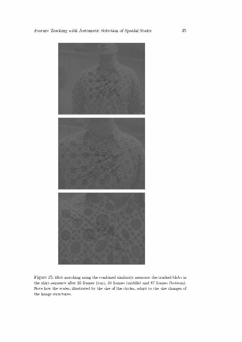
As a further illustration of the capability of the algorithm to track blobsunder large size changes we applied it to a sequence of 87 images where aperson, dressed in a spotted shirt, approaches the camera. In a rectangular areain the initial frame, the 20 most signi�cant blobs were automatically detected,as shown in �gure 14. Figure 15 shows the results after 25, 50 and 87 frameswhen matching on the combined similarity measure. All blobs except one arecorrectly tracked over the entire sequence.

Figure 16 shows the situation after 25 frames when matching on patchsimilarity only. Compared to �gure 15, three more blobs are now lost, and oneblob is mismatched. In scenes like this one, with repetitive, similar structures,the rate of mismatches is considerably higher if we match on patch correlationonly instead of using the combined similarity measure.

When trying to track the blobs at a �xed scale, as can be seen in �gure 17,most of the blobs are lost already after 25 frames. The last correctly trackedblob is lost after about 50 frames.

In summary, these experiments show that similar qualitative properties holdfor blob tracking and for junction tracking: (i) By including the signi�cance val-ues and the selected scale levels in the matching criterion, we obtain a betterperformance than when matching on grey-level correlation only. (ii) The per-formance of tracking at adaptively determined scale levels is superior comparedto similar tracking at a �xed scale.


Let us �nally illustrate how feature tracking with automatic scale selectionover a large number of frames is likely to give us trajectories which correspondto reliable and stable physical scene points or regions of interest on objects.By explicitly registering the features that are stable over time, we are ableto suppress spurious feature responses due to noise, temporary occlusions etc.Figure 18 shows the initial frame of a sequence in which the 10 most signi�cantblobs have been tracked in a region around the face of the subject. The subject�rst approaches the camera and then moves back to the initial position. Figure19 shows the situation after 20, 45 and 90 frames. We can see that after a whileonly four features remain in the feature set and these are the stable featurescorresponding to the nostrils and the eyes. This ability to register stable imagestructures over time is clearly a desirable quality in many computer visionapplications. Notably, for general scenes with large expansions or contractions,a scale selection mechanism is essential to allow for such registrations.


8 Summary and Discussion

We have presented a framework for feature tracking in which a mechanism forautomatic scale selection has been built into the feature detection stage andthe additional attributes of the image features obtained from the scale selectionmodule are used for guiding the other processing steps in the tracking procedure.

We have argued that such a mechanism is essential for any feature trackingprocedure intended to operate in a complex environment, in order to adapt thescale of processing to the size variations that may occur in the image data aswell as over time. If we attempt to track features by processing the image dataat one single scale only, we can hardly expect to be able to follow the featuresover large size variations. This property is a basic consequence of the inherentmulti-scale nature of image structures, which means that a given object mayappear in di�erent ways depending on the scale of observation.

Speci�cally, based on a previously developed feature detection frameworkwith automatic scale selection, we have presented a scheme for tracking cornersand blobs over time in which:

� the image features at any time moment are detected using a feature de-tection method with automatic scale selection, and

� this information is used for

{ guiding the detection and selection of new feature candidates,

{ providing context information for the matching procedure,

{ formulating a similarity measure for matching features over time.

Besides avoiding explicit selection of scale levels for feature detection, the fea-ture detection procedure with automatic scale selection allows us to track imagefeatures over large size variations. As demonstrated in the introductory exam-ple in section 2, we can in this way obtain a substantial improvement in theperformance relative to a �xed-scale feature tracker.

Since the scale levels obtained from the scale selection procedure re ect thespatial extent of the image structures, we can also use this context informationfor avoiding explicit settings of distance thresholds and prede�ned window sizesfor matching. Moreover, by including the scale and signi�cance informationassociated with the image features from the scale selection procedure into amulti-cue similarity measure, we showed how we in this way can improve thereliability of the low-level matching procedure.

Of course, there are inherent limitations in tracking each feature individuallyas done in this work, and as can be seen from the examples, there are a numberof situations where the tracking algorithm fails. Typically, this occurs becauseof rapid changes in the local grey-level pattern around the corner, correspondingto violations of the assumption about small inter-frame motions.

A notable conclusion that can be made in this context, is that despite theselimitations, we have shown by examples that the resulting tracking procedureis able to track most of the visible features that can be followed over timein the sequences presented in this article. By this we argue that the type of


framework presented here provides an important step towards overcoming someof the limitations in previous feature tracking algorithms.

8.1 Spatial consistency and statistical evaluation.

In the scheme presented so far, each feature is tracked individually , without anyexplicit notion of coherently moving clusters. It is obvious that the performanceof a tracking method can be improved if the latter notion can be introduced, andthe overall motion of the clusters can be used for generating better predictions,as well as more re�ned evaluation criteria of matching candidates. To investigateif the motions of the tracked features possibly correspond to the same rigidbody motion, we might compute descriptors such as aÆne 3-D coordinates.Interesting work in this direction have been presented by [Reid and Murray,1993, Wiles and Brady, 1995, Shapiro, 1995].

It is also natural to include a statistical evaluation of the reliability ofmatches as well as their possible agreement with di�erent clusters, as done in[Shapiro, 1995]. Whereas such an approach has not been explored in this work,this should not be interpreted as implying that the scale selection method ex-cludes the usefulness of a statistical evaluation. The main intention behind thiswork has been to explore how far it is possible to reach by using a bottom-upconstruction of feature trajectories and by including a mechanism for automaticscale selection in the feature detection step. Then, the intention is that thesetwo approaches should be applied in a complementary manner, where the scaleselection method serves as a pre-conditioner for generating more reliable hy-potheses with more reliable input data. The scale selection method can alsoprovide context information over what domains statistical evaluations shouldbe made.

8.2 Multi-cue tracking

A tracking method based on a single visual cue, like those reviewed in section1 may have a rather good performance under certain conditions but may failin more complex scenes. In this context, a multi-cue approach to the trackingproblem is natural, i.e a system in which several types of algorithms operatesimultaneously and the algorithm most suitable to a given situation dominates.This means that the vision system must have the ability to evaluate the re-liability of the various tracking methods and to switch between them in anappropriate way.

Initial work in this direction, combining disparity cues with optical owbased object segmentation, has been performed by [Uhlin et al., 1995]. The ap-proach developed here lends itself naturally to integration with such techniques,in which such cues can be used for evaluating candidate feature clusters, andthe feature tracking module in turn can be used as a more re�ned processingmechanism for maintaining object hypotheses over time. Of course, this leads tobasic problems of feature selection. One possible approach for addressing suchproblems has been presented by [Shi and Tomasi, 1994].


8.3 Temporal consistency

As a �nal remark it is worth pointing out that in this work, the image featuresin each frame have been extracted independently from each other and withoutany other explicit use of temporal consistency than the heuristic condition thata feature hypothesis is allowed to survive over a few frames. To make moreexplicit use of temporal consistency, it is natural to incorporate the notion ofa temporal scale-space representation [Lindeberg and Fagerstr�om, 1996] andto include scale selection over the temporal scale domain as well [Lindeberg,1996b].

In this context, it is also natural to combine the feature tracking approachwith a simultaneous calculation of optical ow estimates and to integrate thesetwo approaches so as to make use of their relative advantages. These subjects,including the integration of multiple tracking techniques into a multi-cue frame-work, constitute major goals of our continued research.


References

[Blake et al., 1993] Blake et al. \AÆne-invariant contour tracking with automatic con-trol of spatiotemporal scale". In Proc. 4th International Conference on Computer

Vision, Berlin, Germany, 1993. IEEE Computer Society Press.

[Blom, 1992] J. Blom. Topological and Geometrical Aspects of Image Structure. PhDthesis. , Dept. Med. Phys. Physics, Univ. Utrecht, NL-3508 Utrecht, Netherlands,1992.

[Cipolla and Blake, 1992] R. Cipolla and A. Blake. \Surface orientation and time tocontact from image divergence and deformation". In G. Sandini, editor, Proc. 2ndEuropean Conference on Computer Vision, pages 187{202, Santa Margherita Ligure,Italy, 1992. Springer Verlag, Berlin.

[Curwen et al., 1991] Curwen et al. \Parallel implementation of Lagrangian dynamicsfor real-time snakes". In Proc. British Machine Vision Conference. Springer Verlag,Berlin, 1991.

[Deriche and Giraudon, 1990] R. Deriche and G. Giraudon. \Accurate Corner Detec-tion: An Analytical Study". In Proc. 3rd Int. Conf. on Computer Vision, pages66{70, Osaka, Japan, 1990.

[Faugeras, 1993] O. Faugeras. Three-dimensional computer vision. MIT Press, Cam-bridge, Massachusetts, 1993.

[Florack et al., 1992] L. M. J. Florack; B. M. ter Haar Romeny; J. J. Koenderink, andM. A. Viergever. \Scale and the Di�erential Structure of Images". Image and VisionComputing, 10(6):376{388, Jul. 1992.

[F�orstner and G�ulch, 1987] W. A. F�orstner and E. G�ulch. \A Fast Operator for De-tection and Precise Location of Distinct Points, Corners and Centers of CircularFeatures". In Proc. Intercommission Workshop of the Int. Soc. for Photogrammetry

and Remote Sensing, Interlaken, Switzerland, 1987.

[Gee and Cipolla, 1995] A.H. Gee and R. Cipolla. \Fast visual tracking by tempo-ral consensus". Technical Report CUED/F-INFENG/TR207, Dept of Engineering,University of Cambridge, England, 1995.

[Kitchen and Rosenfeld, 1982] L. Kitchen and A. Rosenfeld. \Gray-Level Corner De-tection". Pattern Recognition Letters, 1(2):95{102, 1982.

[Koenderink and Richards, 1988] J. J. Koenderink and W. Richards. \Two-Dimensional Curvature Operators". J. of the Optical Society of America, 5:7:1136{1141, 1988.

[Koenderink and van Doorn, 1992] J. J. Koenderink and A. J. van Doorn. \Genericneighborhood operators". IEEE Trans. Pattern Analysis and Machine Intell.,14(6):597{605, Jun. 1992.

[Koenderink, 1984] J. J. Koenderink. \The structure of images". Biological Cybernet-ics, 50:363{370, 1984.

[Koller et al., 1994] D. Koller; J. Weber, and J. Malik. \Robust multiple car trackingwith occlusion reasoning". In J.-O. Eklundh, editor, Proc. 3rd European Conference

on Computer Vision, pages 189{196, Stockholm, Sweden, 1994. Springer Verlag,Berlin.

[Lindeberg and Fagerstr�om, 1996] T. Lindeberg and D. Fagerstr�om. \Scale-Space withcausal time direction". In Proc. 4th European Conference on Computer Vision,volume 1064, pages 229{240, Cambridge, UK, April 1996. Springer Verlag, Berlin.


[Lindeberg, 1993] T. Lindeberg. \On Scale Selection for Di�erential Operators". InK. Heia K. A. H�gdra, B. Braathen, editor, Proc. 8th Scandinavian Conf. on Image

Analysis, pages 857{866, Troms�, Norway, May. 1993. Norwegian Society for ImageProcessing and Pattern Recognition.

[Lindeberg, 1994a] T. Lindeberg. \Junction detection with automatic selection of de-tection scales and localization scales". In Proc. 1st International Conference on

Image Processing, volume I, pages 924{928, Austin, Texas, Nov. 1994. IEEE Com-puter Society Press.

[Lindeberg, 1994b] T. Lindeberg. \Scale Selection for Di�erential Operators". Tech-nical Report ISRN KTH/NA/P--94/03--SE, Dept. of Numerical Analysis and Com-puting Science, KTH, Stockholm, Sweden, Jan. 1994. (Submitted).

[Lindeberg, 1994c] T. Lindeberg. Scale-Space Theory in Computer Vision. The KluwerInternational Series in Engineering and Computer Science. Kluwer Academic Pub-lishers, Dordrecht, Netherlands, 1994.

[Lindeberg, 1996a] T. Lindeberg. \Edge detection and ridge detection with automaticscale selection". In Proc. IEEE Comp. Soc. Conf. on Computer Vision and Pat-

tern Recognition, 1996, pages 465{470, San Francisco, California, June 1996. IEEEComputer Society Press.

[Lindeberg, 1996b] T. Lindeberg. \On automatic selection of temporal scales". 1996.

[Meyer and Bouthemy, 1994] F. G. Meyer and P. Bouthemy. \Region-based trackingusing aÆne motion models in long image sequences". Computer Vision, Graphics,

and Image Processing :Image Understanding, 60(2):119{140, 1994.

[Reid and Murray, 1993] I. D. Reid and D. W. Murray. \Tracking foveated cornerclusters using aÆne structure". In Proc. 4th International Conference on Computer

Vision, pages 76{83, Berlin, Germany, 1993. IEEE Computer Society Press.

[Shapiro, 1995] L. S. Shapiro. AÆne analysis of image sequences. Cambridge Univer-sity Press, Cambridge, England, 1995.

[Shapiro et al., 1992a] L. S. Shapiro; H. Wang, and J. M. Brady. \A corner matchingand tracking strategy applied to videophony". Technical Report OUEL 1933/92,Robotics Research Group, University of Oxford, 1992.

[Shapiro et al., 1992b] L. S. Shapiro; H. Wang, and J. M. Brady. \A matching andtracking strategy for independently moving objects". In Proc. British Machine Vi-

sion Conference, pages 306{315. Springer Verlag, Berlin, 1992.

[Shi and Tomasi, 1994] J. Shi and C. Tomasi. \Good features to track". In Proc.

IEEE Comp. Soc. Conf. on Computer Vision and Pattern Recognition, pages 593{600. IEEE Computer Society Press, 1994.

[Smith and Brady, 1995] S. M. Smith and J. M. Brady. \ASSET-2: Real-time motionsegmentation and shape tracking". IEEE Trans. Pattern Analysis and Machine

Intell., 17(8):814{820, 1995.

[Thompson et al., 1993] W. B. Thompson; P. Lechleider, and E. R. Stuck. \Detectingmoving objects using the rigidity constraint". IEEE Trans. Pattern Analysis and

Machine Intell., 15(2):162{165, 1993.

[Uhlin et al., 1995] T. Uhlin; P. Nordlund; A. Maki, and J.-O. Eklundh. \Towardsan Active Visual Observer". In Proc. 5th International Conference on Computer

Vision, pages 679{686, Cambridge, MA, June 1995.


[Wiles and Brady, 1995] C. S. Wiles and M. Brady. \Closing the loop on multiplemotions". In Proc. 5th International Conference on Computer Vision, pages 308{313. IEEE Computer Society Press, 1995.

[Witkin, 1983] A. P. Witkin. \Scale-space �ltering". In Proc. 8th Int. Joint Conf. Art.

Intell., pages 1019{1022, Karlsruhe, West Germany, Aug. 1983.

[Zheng and Chellappa, 1995] Q. Zheng and R. Chellappa. \Automatic feature pointextraction and tracking in image sequences for arbitrary camera motion". Interna-tional Journal of Computer Vision, 15(1):31{76, 1995.


A Algorithmic details

This appendix gives a detailed listing of the parameters that in uence the algorithmas well as the parameter settings that have been used for generating the experiments.

A.1 Prediction

The parameters determining the size of the search window (see section 6) were

ksize = 5

kw1 = 1:5

kw2 = 2 � kw1

Dmin = 16

A.2 Feature detection

When detecting features with automatic scale selection, the following scale ranges wereused in the initial frame:

Junction detection Blob detection

tmin = 4:0 tmin = 4:0tmax = 256:0 tmax = 512:0

and the parameter in the normalized derivative concept (see section 3) was set to:


= 0:875 = 1

When searching for new image features, the search for matching candidates to a featuredetected at scale tdet was performed in the interval [tdet=k1; tdetk1], where krange = 3.

In all experiments, the sampling density in the scale direction was set to correspondto a minimum of 5 scale levels per octave. In all other aspects, the feature detectionalgorithms followed the default implementation of junction and blob detection withautomatic scale selection described in [Lindeberg, 1994b]. The maximum number ofmatching candidates evaluated for each feature was:


n = 8 n = 20

A.3 Matching

The following thresholds were used in the matching step


Tpatch = 0:75 Tpatch = 0:6Tcomb = 0:65 Tcomb = 0:5

and the parameters for controlling the quality measure over time (see section 6)

dqi = 0:2

dqd = 0:1

Tq = 0


Similarity measures: Relative weights In the experiments presented here, the fol-lowing relative weights (see section 5) were used in the combined signi�cance measure(15):


cpatch = 1:0 cpatch = 1:0csign = �0:08 csign = �0:25cscale = �0:08 cscale = �0:08cpos = �0:1 cpos = �0:1

To give a qualitative motivation for using these orders of magnitude for the relativeweights, let us �rst estimate the ranges in which these descriptors will vary:

� For the cross-correlation measure, it trivially holds that jSpatchj < 1. By thethresholding operation on this value, jTpatchj = 0:7, the variation of this entityis con�ned to the interval jSpatchj 2 [0:7; 1:0]. In practice, the relative variationsare usually in the interval jSpatchj 2 [0:8; 1:0].

� Concerning the signi�cance measure, the signi�cance values of corners computedfrom an image with grey-level values in the range [0; 255] typically vary in theinterval logR < 25. Empirically, the relative variations are usually of the orderof � logR < 3. For blob features, the corresponding values are logR < 8 and� logR < 1.

� Concerning the stability of the scale values, the restricted search range given bykrange, implies that the relative variation of this descriptor will always be lessthan � log t � 1.

� For the proximity measure the maximum value isp2 � 0:5 � krange � kw1 � 5.

With smooth scene motions the value is normally considerably smaller.

Motivated by the fact that the relative variation in Spatch is about a factor of tensmaller than the other entities, the relative weights of the components in Scomb wereset according to the table above.

Note that the correlation measure is the dominant component, and the relativein uence of the other components corresponds to about half that variation.

The reason why csign is increased in blob detection, is that the dimension of thesigni�cance measures are di�erent:

[~�2 �norm] = [brightness]6

[(r2

normL)2] = [brightness]2

Hence, it is natural to increase the coeÆcient of Ssign = j log RBRA

j by a factor of three inblob detection compared to junction detection. As a general rule, we have not performedany �ne-tuning of the parameters, and all parameter values have been the same in allexperiments.


Initial frame

Fixed scale tracking Adaptive scale tracking

Figure 1: Illustration of the importance of automatic scale selection when tracking

image structures over time. The corner is lost using detection at a �xed scale (left

column), whereas it is correctly tracked using adaptive scale selection (right column).

The size of the circles correspond to the detection scales of the corner features.


Figure 2: The result of applying the corner detection algorithm with automaticscale selection to two di�erent grey-level images. (top row) Original grey-levelimages. (bottom row) The 100 most signi�cant corners superimposed onto abright copy of the original image. Graphically, each corner is illustrated bycircle with the radius re ecting the detection scale. Observe that a reasonableset of junction candidates is obtained, and that the circles serve as naturalregions of interest around the corners to be used in further processing.

Figure 3: The result of applying the blob detection algorithm with automaticscale selection to the same images as used for corner detection in �gure 2. The100 most signi�cant blobs have been graphically illustrated by circles with theirradius proportional to the detection scale.


Algorithm:

For each frame:

For each feature F in the feature set:

1. Prediction

1.1 Predict the position of the feature F in the current frame based oninformation from the previous frames.

1.2 Compute the search region in the current frame based on informationfrom the previous frames and the scale of the feature.

2. Detection

Detect n candidates Ck over a reduced set of scales in the region ofinterest in the current frame.

3. Matching

3.1 Match every candidate Ck to the feature F and �nd the best matchusing the combined similarity measure.

3.2 Optionally, perform bidirectional matching to register safe matches.

3.3 Compare the similarity value to a predetermined threshold:If above: consider the feature as matched; update its position, itsscale descriptor, its signi�cance value, its grey-level patch and in-crease its quality value.If below: consider the feature as unmatched; update its position tothe predicted position and decrease its quality value.

Parse the feature set to detect feature merges and remove features havingquality values below a certain threshold.

Figure 4: Overview of the feature tracking algorithm.


Figure 5: The phone sequence: The initial frame with 14 detected corners.


Figure 6: Corner tracking with adaptive scale selection and matching on combined

similarity: the tracked corners in the phone sequence after 30 frames (top), 50 (middle)

and 60 frames (bottom). As can be seen, all corners are correctly tracked.


Figure 7: Corner tracking with �xed scales over time: the tracked corners in phone

sequence after 30 frames (top), 50 (middle) and 60 frames (bottom). Note that the

blunt corners are lost compared to the adaptive scale tracking in �gure 6.


Figure 8: The train sequence: The initial frame with 29 detected corners.


Figure 9: Corner tracking with adaptive scale selection and matching on combined

similarity: the tracked corners in the train sequence after 60 frames (top), 100 (middle)

and 140 frames (bottom).


Figure 10: Matching candidates on patch correlation only: the tracked corners in the

train sequence after 60 frames (top) and 100 frames (bottom). Three more corners are

lost as compared to �gure 9.


Figure 11: The train sequence: The initial frame with 13 detected blobs. (The size of

the circles correspond to the detection scales of the blob features.


Figure 12: Blob tracking with adaptive scale selection and matching on combined

similarity: the tracked blobs in the train sequence after 30 frames (top), 90 (middle)

and 150 frames (bottom). All blobs are correctly tracked.


Figure 13: Blob tracking using �xed scales in the detection procedure: the tracked

blobs in train sequence after 30 frames (top), 90 (middle) and 150 frames (bottom).

Only one blob is correctly tracked over the whole sequence.


Figure 14: The initial frame of the shirt sequence with the 20 strongest blobs detected

in a rectangular window. The size of the circles correspond to the detection scales of

the blob features.)


Figure 15: Blob matching using the combined similarity measure: the tracked blobs in

the shirt sequence after 25 frames (top), 50 frames (middle) and 87 frames (bottom).

Note how the scales, illustrated by the size of the circles, adapt to the size changes of

the image structures.


Figure 16: Matching the candidates on patch similarity only: the tracked blobs in the

shirt sequence after 25 frames. Compared to the top image in �gure 15, three more

blobs are lost and one is mismatched.

Figure 17: Blob tracking using �xed scales in the detection procedure: the tracked

blobs in the shirt sequence after 25 frames. Most blobs are already lost because they

no longer exist at the initially chosen scale.


Figure 18: The initial frame of the face sequence with the 10 most signi�cant blobs

detected in a region around the face of the subject.


Figure 19: Tracking the blobs in the face sequence with automatic scale selection; the

situation after 20, 45 and 90 frames. After about 60 frames only the 4 most stable blobs

remain in the feature set.

Feature Tracking with Automatic selection of spatial - DiVA Portal

Documents

Transcript of Feature Tracking with Automatic selection of spatial - DiVA Portal