FEATURE SELECTION METHODS FOR SUPPORT VECTOR …

The Pennsylvania State University

The Graduate School

Department of Electrical Engineering

FEATURE SELECTION METHODS

FOR SUPPORT VECTOR MACHINES

FOR TWO OR MORE CLASSES,

WITH APPLICATIONS TO THE ANALYSIS OF

ALZHEIMER’S DISEASE AND ITS ONSET

WITH MRI BRAIN IMAGE PROCESSING

A Dissertation in

Electrical Engineering

by

Yaman Aksu

c© 2010 Yaman Aksu

Submitted in Partial Fulfillmentof the Requirements

for the Degree of

Doctor of Philosophy

August 2010

The dissertation of Yaman Aksu was reviewed and approved* by the following:

Kenneth JenkinsProfessor of Electrical EngineeringHead of the Department of Electrical Engineering

David J. MillerProfessor of Electrical EngineeringDissertation Co-AdvisorCo-Chair of Committee

Qing X. YangProfessor of Radiology and NeurosurgeryCo-Chair of Committee

George KesidisProfessor of Electrical Engineeringand Computer Science and EngineeringDissertation Co-Advisor

Constantino M. LagoaAssociate Professor of Electrical Engineering

James WangProfessor of Information Sciences and Technology

*Signatures on file in the Graduate School.

iii

Abstract

Feature selection for classification in high-dimensional spaces can improve generalization,reduce classifier complexity, and identify important, discriminating feature “markers”. For sup-port vector machine (SVM) classification, a widely used technique is Recursive Feature Elim-ination (RFE). We demonstrate RFE is not consistent with margin maximization, central tothe SVM learning approach. We thus propose explicit margin-based feature elimination (MFE)for SVMs and show both improved margin and improved generalization, compared with RFE.Moreover, for the case of a nonlinear kernel, we show RFE assumes the squared weight vector2-norm is strictly decreasing as features are eliminated. We demonstrate this is not true for theGaussian kernel and, consequently, RFE may give poor results in this case. We show that MFEfor nonlinear kernels gives better margin and generalization. We also present an extension whichachieves further margin gains, by optimizing only two degrees of freedom – the hyperplane’sintercept and its squared 2-norm – with the weight vector orientation fixed. We finally introducean extension that allows margin slackness. We compare against several alternatives, includingRFE and a linear programming method that embeds feature selection within the classifier design.On high-dimensional gene microarray data sets, UC Irvine repository data sets, and Alzheimer’sdisease brain image data, MFE methods give promising results. We then develop several MFE-based feature elimination methods for the case of more than two classes (the “multiclass” case).We compare against RFE-based multiclass feature elimination and show that our MFE-basedmethods again consistently achieve better generalization performance. In summary, we identifysome difficulties with the well-known RFE method, especially in the kernel case, develop novel,margin-based feature selection methods for linear and kernel-based two-class and multiclass dis-criminant functions for support vector machines (SVMs) addressing separable and nonseparablecontexts, and provide an objective experimental comparison of several feature selection methods,which also evaluates consistency between a classifier’s margin and its generalization accuracy.

We then apply our SVM classification and MFE methods to the challenging problem ofpredicting the onset of Alzheimer’s Disease (AD), focusing on predicting conversion from MildCognitive Impairment (MCI) to AD using only a single, first-visit MRI for the person so as to aimfor early diagnosis. In addition, we apply MFE for selecting brain regions as disease “biomarkers”.For these aims, for the pre-classification image data preparation step, we co-develop an MRIbrain image processing pipeline system named STAMPS, as well as develop a related systemwith additional capabilities named STAMPYS. These systems utilize external standard MRIbrain image processing tools and generate output image types particularly suitable for detecting(and encoding) brain atrophy for Alzheimer’s disease. We identify and remedy some basic MRIimage processing problems caused by some limitations of external tools used in STAMPS – i.e.we introduce our basic fv (fill ventricle) algorithm for ventricle segmentation of cerebrospinalfluid (CSF). For prediction of conversion to AD for MCI patients, we demonstrate that our earlydiagnosis system achieves higher accuracy than similar recently published methods.

iv

Table of Contents

List of Tables . . . . . . . . . . . . . . . . . . . . . . . . . . . . . . . . . . . . . . . . . . . vi

List of Figures . . . . . . . . . . . . . . . . . . . . . . . . . . . . . . . . . . . . . . . . . . vii

Acknowledgments . . . . . . . . . . . . . . . . . . . . . . . . . . . . . . . . . . . . . . . . ix

Chapter 1. Introduction . . . . . . . . . . . . . . . . . . . . . . . . . . . . . . . . . . . . . 11.1 Statistical Learning Theory and learning machines . . . . . . . . . . . . . . . 11.2 VC dimension and Structural Risk Minimization (SRM) . . . . . . . . . . . . 21.3 Brief review of Support Vector Machines (SVMs) . . . . . . . . . . . . . . . . 31.4 SVM and SRM . . . . . . . . . . . . . . . . . . . . . . . . . . . . . . . . . . . 51.5 Feature selection in classification . . . . . . . . . . . . . . . . . . . . . . . . . 61.6 Feature selection for SVMs . . . . . . . . . . . . . . . . . . . . . . . . . . . . 91.7 Contributions of this thesis . . . . . . . . . . . . . . . . . . . . . . . . . . . . 10

Chapter 2. Margin-maximizing feature selection methods for Support Vector Machines:two-class case . . . . . . . . . . . . . . . . . . . . . . . . . . . . . . . . . . . . 12

2.1 RFE and limitations of RFE . . . . . . . . . . . . . . . . . . . . . . . . . . . . 122.1.1 RFE and limitations of RFE: linear kernel case . . . . . . . . . . . . . 122.1.2 RFE and limitations of RFE: nonlinear kernel case . . . . . . . . . . . 12

2.2 MFE: direct margin-based feature elimination . . . . . . . . . . . . . . . . . . 142.2.1 MFE for the linear kernel case . . . . . . . . . . . . . . . . . . . . . . 14

2.2.1.1 MFE algorithm pseudocode for SVMs: linear kernel case . . 152.2.2 MFE for the nonlinear kernel case . . . . . . . . . . . . . . . . . . . . 162.2.3 “Little Optimization” (LO): further increases in margin . . . . . . . . 18

2.3 MFE-slack: utilizing margin slackness . . . . . . . . . . . . . . . . . . . . . . 202.3.1 MFE-slack algorithm pseudocode for linear and nonlinear kernel SVMs 22

2.4 Results . . . . . . . . . . . . . . . . . . . . . . . . . . . . . . . . . . . . . . . . 222.4.1 Experimental procedure for the initial classifier training . . . . . . . . 22

2.4.1.1 Data pre-processing prior to initial classifier training . . . . . 232.4.2 Experimental procedure for feature elimination . . . . . . . . . . . . . 23

2.4.2.1 Stopping criteria . . . . . . . . . . . . . . . . . . . . . . . . . 242.4.3 Experiments on high-dimensional separable data . . . . . . . . . . . . 262.4.4 Experiments on low-dimensional separable data . . . . . . . . . . . . . 282.4.5 Experiments on low-dimensional nonseparable data . . . . . . . . . . . 302.4.6 High-dimensional feature space application: brain images . . . . . . . 30

2.5 Conclusions . . . . . . . . . . . . . . . . . . . . . . . . . . . . . . . . . . . . . 33

Chapter 3. Margin-maximizing feature selection methods: “multiclass” case (k > 2) . . . 353.1 Introduction . . . . . . . . . . . . . . . . . . . . . . . . . . . . . . . . . . . . . 353.2 Brief summary of multiclass SVMs . . . . . . . . . . . . . . . . . . . . . . . . 353.3 Multiclass RFE-based methods . . . . . . . . . . . . . . . . . . . . . . . . . . 373.4 Multiclass MFE methods . . . . . . . . . . . . . . . . . . . . . . . . . . . . . 37

3.4.1 Pseudocode for algorithms MFE-k-G, MFE-k-SP, and MFE-k-SC, forlinear and nonlinear kernel-based multiclass SVMs . . . . . . . . . . . 38

3.5 Multiclass MFE-slack: utilizing margin slackness . . . . . . . . . . . . . . . . 393.5.1 MFE-k-SP-slack . . . . . . . . . . . . . . . . . . . . . . . . . . . . . . 39

v

3.5.1.1 MFE-k-SP-slack algorithm pseudocode for linear and nonlin-ear kernel-based SVMs . . . . . . . . . . . . . . . . . . . . . 40

3.5.2 MFE-k-G-slack . . . . . . . . . . . . . . . . . . . . . . . . . . . . . . . 423.5.2.1 MFE-k-G-slack-s algorithm pseudocode for linear and non-

linear kernel-based SVMs . . . . . . . . . . . . . . . . . . . . 423.5.2.2 MFE-k-G-slack-m algorithm pseudocode for linear and non-

linear kernel-based SVMs . . . . . . . . . . . . . . . . . . . . 433.5.3 MFE-k-SC-slack . . . . . . . . . . . . . . . . . . . . . . . . . . . . . . 43

3.5.3.1 MFE-k-SC-slack-s algorithm pseudocode for linear and non-linear kernel-based SVMs . . . . . . . . . . . . . . . . . . . . 44

3.5.3.2 MFE-k-SC-slack-m algorithm pseudocode for linear and non-linear kernel-based SVMs . . . . . . . . . . . . . . . . . . . . 45

3.6 MFE-k-Kesler . . . . . . . . . . . . . . . . . . . . . . . . . . . . . . . . . . . . 453.6.1 Kesler construction . . . . . . . . . . . . . . . . . . . . . . . . . . . . . 453.6.2 MFE-k-Kesler . . . . . . . . . . . . . . . . . . . . . . . . . . . . . . . . 46

3.7 Results . . . . . . . . . . . . . . . . . . . . . . . . . . . . . . . . . . . . . . . . 46

Chapter 4. MRI brain image processing and analysis of Alzheimer’s disease and its onset 504.1 Introduction . . . . . . . . . . . . . . . . . . . . . . . . . . . . . . . . . . . . . 504.2 Brain MR image processing pipeline . . . . . . . . . . . . . . . . . . . . . . . 544.3 Results . . . . . . . . . . . . . . . . . . . . . . . . . . . . . . . . . . . . . . . . 57

4.3.1 ADNI data . . . . . . . . . . . . . . . . . . . . . . . . . . . . . . . . . 574.3.2 ROI-based and voxel-based experiments . . . . . . . . . . . . . . . . . 574.3.3 Procedure for initial classifier training for AD/MCI/Control data . . . 584.3.4 Classifier 1: Control-AD123 classifier . . . . . . . . . . . . . . . . . . . 59

4.3.4.1 Classifier 1R: features are ROI-based . . . . . . . . . . . . . 594.3.4.2 Classifier 1V: features are voxel-based . . . . . . . . . . . . . 59

4.3.5 Classifier 2: MCIncc-MCIcc (nonconverters-by-CDR vs. converters-by-CDR) . . . . . . . . . . . . . . . . . . . . . . . . . . . . . . . . . . 644.3.5.1 Classifier 2R: features are ROI-based . . . . . . . . . . . . . 64

4.3.6 Classifier 3: MCInct-MCIct (nonconverters-by-trajectory vs. converters-by-trajectory) . . . . . . . . . . . . . . . . . . . . . . . . . . . . . . . 644.3.6.1 Classifier 3R: features are ROI-based . . . . . . . . . . . . . 654.3.6.2 Classifier 3V: features are voxel-based . . . . . . . . . . . . . 69

4.3.7 Comparison with statistical paired t-test using SPM5 . . . . . . . . . 694.4 Conclusions . . . . . . . . . . . . . . . . . . . . . . . . . . . . . . . . . . . . . 784.5 Acknowledgement . . . . . . . . . . . . . . . . . . . . . . . . . . . . . . . . . . 79

Appendix A. Software we created . . . . . . . . . . . . . . . . . . . . . . . . . . . . . . . 80A.1 SVMcatalyst software . . . . . . . . . . . . . . . . . . . . . . . . . . . . . . . 80A.2 fv algorithm and tool for ventricle segmentation of CSF . . . . . . . . . . . . 80

A.2.1 fv algorithm . . . . . . . . . . . . . . . . . . . . . . . . . . . . . . . . . 80A.2.2 fv tool . . . . . . . . . . . . . . . . . . . . . . . . . . . . . . . . . . . . 82

A.3 STAMPS software . . . . . . . . . . . . . . . . . . . . . . . . . . . . . . . . . 83

Appendix B. . . . . . . . . . . . . . . . . . . . . . . . . . . . . . . . . . . . . . . . . . . 84B.0.1 Exhaustive Subsampling Approach (ESA) and Hierarchical MFE (H-

MFE) . . . . . . . . . . . . . . . . . . . . . . . . . . . . . . . . . . . . 84

Appendix C. HAMMER method . . . . . . . . . . . . . . . . . . . . . . . . . . . . . . . . 85

Bibliography . . . . . . . . . . . . . . . . . . . . . . . . . . . . . . . . . . . . . . . . . . . 86

vi

List of Tables

4.1 Results for ROI-based Classifiers 1R and 2R. . . . . . . . . . . . . . . . . . . . . 604.2 Results for voxel-based Classifier 1V. . . . . . . . . . . . . . . . . . . . . . . . . . 614.3 Results for voxel-based Classifier 1Vb. . . . . . . . . . . . . . . . . . . . . . . . . 624.4 Results for ROI-based Classifier 3R. Part 1 of 2. . . . . . . . . . . . . . . . . . . 674.5 Results for ROI-based Classifier 3R. Part 2 of 2. . . . . . . . . . . . . . . . . . . 684.6 Results for voxel-based Classifier 3V. . . . . . . . . . . . . . . . . . . . . . . . . . 69

vii

List of Figures

2.1 Counterexample for RFE. . . . . . . . . . . . . . . . . . . . . . . . . . . . . . . . 132.2 Results for the Gaussian kernel for MFE and RFE. . . . . . . . . . . . . . . . . . 162.3 Training set margin, test set error rate, for comparing MFE and RFE. . . . . . . 172.4 Illustration for solution of the “little optimization (LO)” problem. . . . . . . . . 192.5 Illustrative example for MFE-slack. . . . . . . . . . . . . . . . . . . . . . . . . . . 212.6 Results with linear kernel for three high-dimensional (gene microarray) data sets. 252.7 Results with polynomial kernel for a high-dimensional (gene microarray) data set. 262.8 Comparison of single trials for MFE and NLPSVM. . . . . . . . . . . . . . . . . 292.9 Results for multiple kernel types for separable low-d data sets. . . . . . . . . . . 312.10 Results for multiple kernel types for nonseparable low-d data sets. . . . . . . . . 322.11 Initial illustrative MFE and RFE curves for brain image data. . . . . . . . . . . . 332.12 Initial illustrative MFE and RFE results for brain image data. . . . . . . . . . . 34

3.1 Illustration of MFE-k and MFE-k-slack methods. . . . . . . . . . . . . . . . . . . 413.2 Results for linear kernel for multiclass MFE and MSVM-RFE-WW. . . . . . . . 483.3 Results for MFE-k-Kesler. . . . . . . . . . . . . . . . . . . . . . . . . . . . . . . . 49

4.1 Trajectory results for ROI-based Classifier 1R. . . . . . . . . . . . . . . . . . . . 534.2 Regions found by MFE with Classifier 1V. . . . . . . . . . . . . . . . . . . . . . . 624.3 Trajectory results for voxel-based Classifier 1V. . . . . . . . . . . . . . . . . . . . 634.4 Paired t-test results for AD/Control groups for gray matter: all p values (uncor-

rected). . . . . . . . . . . . . . . . . . . . . . . . . . . . . . . . . . . . . . . . . . 714.5 Paired t-test results for AD/Control groups for gray matter: p < 0.0001 uncorrected 734.6 Paired t-test results for AD/Control groups for white matter: p < 0.0001 uncor-

rected . . . . . . . . . . . . . . . . . . . . . . . . . . . . . . . . . . . . . . . . . . 744.7 Paired t-test results for AD/Control groups for gray matter: FDR-corrected . . . 764.8 Paired t-test results for AD/Control groups for gray matter: FDR-corrected (ortho) 77

A.1 Illustration of problematic scenario with ventricles partly mislabeled as CSF. . . 80

viii

Notation

R the set of real numbersN the set of natural numbersM number of features (pre-elimination)N number of training samplesx training vector, aka training sampleX set x1, . . . , xN of training vectorsT number of support vectorsS set 1, . . . , T of indexes for support vectorss support vector ∈ X, e.g. sl is lth support vector with l ∈ Sk number of classesy class label ∈ ±1 for two-class caseyn y of xn

yx y of x, e.g. yslis y of sl

p class label ∈ 1, . . . , k for multiclass casepn p of xn

p(·, ·) probability density function (pdf)cn minimum-signed-distance class for sample xn in multiclass SVMw weight vectorb offset, aka intercept, aka affine parameterδ or ∆ delta, a quantity computed by the MFE method herein〈· , ·〉 inner productφ(·) mapping into feature space, possibly infinite-dimensionalK(·, ·) kernel functionF space induced by a kernelf(·) discriminant functionξ slackness variableγ marginλ Lagrange multiplier (uses same subscripting as y above)ζn,p binary (indicator) variable; 1 if pn (the class of xn) is p, 0 otherwise.Λ Lagrange coefficient, calculated from multiple Lagrange multipliers in multiclass SVMsC regularization parameter for SVMsX space of inputs for a learning machineY space of outputs for a learning machinex input to a learning machine (x ∈ X ), such as a training vector xy output of a learning machine (y ∈ Y), such as a class label yh VC dimensionL(·, ·) loss functionR(·) expected riskRemp(·) empirical risk(kl

)number of combinations (k-choose-l), aka binomial coefficient

ix

Acknowledgments

For all of their help and guidance, I am grateful to my thesis co-advisor and committeeco-chair Prof. David Miller, thesis co-advisor Prof. George Kesidis, and committee co-chair Prof.Qing Yang, who were also my three supervisors. I am grateful to my committee members Prof.Constantino Lagoa and Prof. James Wang. Many thanks to Dr. Don Bigler, for our collaborationin creating and using the STAMPS software and for a number of useful discussions on MRI brainimages and their processing, and to everyone who helped me at PSU.

1

Chapter 1

Introduction

1.1 Statistical Learning Theory and learning machines

Statistical learning theory is concerned with producing a function f : X → Y that esti-mates from an input x ∈ X an output y ∈ Y considered to be the “truth” associated with x.For instance, x may be a vector x ∈ RM (M ∈ N) of observables and y the class y ∈ ±1 thatx belongs to. More precisely, a “learning machine” is defined by a family of possible mappingsx 7→ f(x,Θ) parameterized by Θ, with “learning” (aka training) being the step of employing a“training set” X of input samples in order to choose a particular Θ value1 whereby one is simplyleft with the desired mapping x 7→ f(x).

“Generalization” refers to the ability to estimate the “true” output for a previously un-seen (“test”) x sample (which was not employed by the training). Related to generalization isthe notion of “capacity” of the learning machine, an abstract concept that simply refers to themachine’s ability to learn any training set without error.2 For example, trained on data aboutvehicles, such as images of vehicles, a machine that declares a bicycle is a car because it has wheelsis a machine whose capacity is too small, whereas a machine that declares that a two-door redcar with round headlights is not a car because of not being white with four doors and rectan-gular headlights is a machine whose capacity is too large. By finding the right balance betweenaccuracy obtained on a particular training set and capacity, best generalization performance canbe achieved. Capacity is made concrete using a measure, a non-negative integer, called the VCdimension (Vapnik Chervonenkis dimension) – the VC dimension is a property of a family offunctions and is discussed shortly.

When y values for the training samples are provided to the learning (as available ground-truth), the learning is called “supervised” – otherwise it is called “unsupervised”. The generalassumption is that x and y are drawn from an unknown cumulative probability distributionP (x,y). Based on the idea of a loss function L : Y ×Y → R, the loss (i.e. penalty) of making anincorrect decision f(x, Θ) when the true output is ytrue is L(f(x,Θ),ytrue) – thus the expectedrisk is stated as:

R(Θ) =∫

X ,Y

L(f(x, Θ),y)dP (x,y). (1.1)

Four components (75) are needed for building a learning machine. The first component isthe domain, which is the learning problem with its associated loss function L(·, ·) – for example,classification, regression (or regression estimation), and probability density estimation are differ-ent problems of function estimation i.e. different learning problems. In classification, Y is a setof k classes (categories), and L(u, v) is 1 if u = v, and is 0 otherwise – for example, if Y = ±1,L(u, v) is 1

2 |v − u|. In regression, Y = R, and one can similarly use L(u, v) ≡ |v − u|. In densityestimation, L(f(x, Θ), p) ≡ − log(p(x)) can be used, where p is the density being estimated.

1Θ is a set of parameters called “hyperparameters”. A Θ value is a set of hyperparameter values.

2Caution: Terminology is not ideal – normally an excess of “ability” or “capacity”, such as in humans,

would not result in poor performance, whereas in the machine context too much capacity is essentiallyassociated with resulting poor performance e.g. in the form of data overfitting (a type of undesirable“overlearning” of the data).

2

The second component needed for building a learning machine is an induction principle fordefining a decision rule. The optimal f in (1.1) is the one that minimizes the expected risk R(Θ).As established by Bayesian decision theory, the Bayesian decision minimizes the expected riskR(Θ) and is thus optimal (20). Thus, in the event one has complete knowledge of the probabilitydensity function p(x,y) (and thus dP (x,y) which is p(x,y)dxdy), using the Bayesian approachone would be able to infer the optimal f (20; 28). However, very often in practice p(x,y) is notavailable, and even though one could compute its estimate p(x,y), this estimation is a difficultstep and will at best yield a suboptimal result limited by the richness of the training data (20; 28).Requiring neither this estimation nor a priori knowledge about the probability distribution (e.g.the analytic form of p(x,y)), statistical learning theory approaches the problem of analyzing theexpected risk via generating bounds for it. The bound analysis is an integral part of the maininduction principle in statistical learning theory, named Structural Risk Minimization (SRM),discussed below in Sec. 1.2.

The final two of the four components for building a learning machine (75), which are 3) aset of decision functions, and 4) an algorithm for implementing the first three components (1-3),depend on the particular choice of learning formulation and thus our discussion of them will beaddressed throughout this thesis.

1.2 VC dimension and Structural Risk Minimization (SRM)

VC dimension is a property of a parameterized family of functions f(Θ) (discussed inSec. 1.1). Suppose there is a set of N observations X = x1, . . . , xN with associated “truth”Y = y1, . . . , yN. Since in this thesis we focus on the classification problem, we now convey aconcrete definition for VC dimension by focusing on the two-class classification problem as anexample. Given a family of functions f(Θ), if one can find, for each of the 2N possible ways oflabeling the N points, a family member able to correctly assign this particular labeling to the Npoints, we say (using terminology of (6)) that this set of points is “shattered” by this family. TheVC dimension is defined as the maximum number of points that the family can shatter (6). TheVC dimension of the family being h does not mean that every set of h points can be shatteredby this family (6). The partitioning of the data space by a hyperplane into two half-spaces isreferred to as a “linear dichotomy”, and the VC dimension of a set of hyperplanes in RM is M +1(6).

Suppose L(·, ·) only takes the values 0 and 1, and L(u, v) is 12 |v − u| as stated above, as

this thesis will focus on classification. Given the sets X and Y above, the bound (1.2) holds withprobability 1− η (where 0 ≤ η ≤ 1 can be chosen arbitrarily small) for a learning machine withVC dimension h (69):

R(Θ) ≤ Remp(Θ) +

√h(log(2N/h) + 1)− log(η/4)

N. (1.2)

The second term on the right-hand side, which contains the VC dimension, is called the VCconfidence. Remp(Θ), given by (1.3), is the “empirical risk”, the mean error rate measured onthe training set.

Remp(Θ) =1

2N

N∑n=1

|yn − f(xn, Θ)| (1.3)

Since Remp(Θ) is a fixed number for a given choice of training set xn, yn and the Θ chosen bythe training, the right-hand side of (1.2), which is independent of P (x,y), can be calculated ifone knows h – the underlying assumption is that the training data and the test data are drawnindependently according to some P (x,y) (6). Thus, a principled way of choosing a learningmachine is to choose from among a set of candidates the one with the lowest value for the right-hand side of (1.2). To minimize the right-hand side, there is a tradeoff between minimizing the

3

training error and the VC confidence depending on the complexity of the machine through themachine capacity measure h. The induction principle Structured Risk Minimization (SRM) hasbeen defined so as to introduce a “structure” into the candidate set F cands by considering nestedsubsets F1 ⊂ F2 ⊂ . . . ⊂ FZ (for some integer Z, with FZ ⊆ F cands) with associated known VCdimensions h1 < h2 < . . . < hZ (or known bounds on the VC dimensions). In this way, for a givensubset Fi, the goal would be to minimize the empirical risk Remp among members of that subset.Accordingly, upon training a number of machines across subsets (possibly as few as simply onemachine per subset), one can simply choose the machine with the least sum of empirical riskRemp and VC confidence. The bound is guaranteed not tight when the VC confidence, whichmonotonically increases with h, exceeds a threshold (which, clearly, would be relative to themaximum value chosen for the loss function) – for example, for the 0-1 loss defined above, areasonable threshold is 1.3 Overall the bound (1.2) is simply a guide – among two machinesachieving zero empirical risk, it is possible for the one with the higher VC dimension to achievebetter generalization performance. The bound is not valid for infinite VC dimension, which, bydefinition, refers to the ability to shatter an arbitrarily large number of points. Note, however,that machines from a family of infinite VC dimension are not guaranteed to generalize poorly –for example, the k-nearest-neighbor classifier, which classifies a sample by voting based on labelsof its k nearest neighbors. Along this line, (43; 44) introduced the NNSRM (nearest-neighbor-SRM) classifier which focuses on combining the power of the SRM principle with the versatilityof the NN classifier – the classifier is proposed as a guaranteed-to-converge and computationallyless expensive alternative to the Support Vector Machine (SVM) which, to be discussed shortly,is “one of the first practical learning procedures for which useful bounds on the VC dimensioncould be obtained and hence the SRM program could be carried out” (39).

Additional examples on the VC dimension, including examples discussing it in the contextof a function family’s number of parameters, can be found in (6). Next, in Sec. 1.3, we give a briefreview of Support Vector Machines (SVMs), which will also serve to lead into our subsequentdiscussion of the connection between SRM and SVM in Sec. 1.4.

1.3 Brief review of Support Vector Machines (SVMs)

Consider a labeled training set (xn, yn), n = 1, . . . , N, where yn ∈ ±1 is the classlabel and xn = (xn,1, . . . , xn,M ) ∈ RM is the n-th data sample. A hyperplane acting as a binary(two-class) decision function in this M -dimensional space is defined by f(x) ≡ wTx + b = 0,w ∈ RM , b ∈ R. Denoting g(xn) ≡ ynf(xn), the signed distance from a data point xn to thedecision boundary is g(xn)

||w|| . The decision boundary is a separating one if it satisfies g(xn) > 0

for all xn. The margin of the separating decision boundary is thus defined as γ ≡ minn g(xn)

||w|| .A support vector machine (SVM) is a linear or generalized linear two-class classifier that learnsa separator for the training set with maximum margin. The “support vectors”, used to specifythe SVM solution, which we denote by s1, ..., sT (with index set S = 1, 2, ..., T), are asubset of the training points at margin distance to the decision boundary. In the linear case,the SVM weight vector solution is w ≡ ∑

k∈Sλsk

ysksk, where λsk

are scalar (positive) Lagrange

multipliers. In the generalized linear (nonlinear) case, f(x) ≡ wTφ(x) + b = 0, w ∈ RL, b ∈ R,φ(x) ≡ [φ1(x), φ2(x), . . . , φL(x)]T, with φi(x) nonlinear functions of the x coordinates. Ofparticular interest is when inner products between φ(x) and φ(u) can be efficiently computed viaa positive definite kernel function, K(x, u) ≡ φT(x)φ(u). In this case, both φ(·) and w itself need

3For example, for this case, (6) plotted the VC confidence versus h/N for N = 10, 000 and η = 0.05

as well as illustrated that the VC confidence exceeds 1 for h/N > 0.37.

4

not be explicitly defined since both the SVM discriminant function f(·) and the SVM weightvector squared 2-norm can be expressed solely in terms of the kernel, i.e.:

f(x) =∑

k∈Sλsk

yskK(sk, x) + b, (1.4)

||w||2 =∑

k∈S

∑

l∈Sλsk

yskλsl

yslK(sk, sl). (1.5)

This approach (the “kernel trick”), where K(·, ·) is explicitly specified and provided to the SVMtraining, is referred to as the “nonlinear kernel case”.

For both linear or nonlinear kernels, the basic SVM training problem is:

minw,b

12||w||2 s.t. ynf(xn) ≥ 1, n = 1, . . . , N (1.6)

Recall that f(xn) in the constraints in (1.6) simply stands for wTx + b in the linear case and〈w, φ(x)〉+b in the nonlinear kernel case – that is, as (1.6) states the basic SVM training problemconveniently for both cases, it is important to keep in mind w and b indeed appear in theconstraints. The relationship of (1.6) to margin maximization can be understood as follows (3).Assuming we have a separator (i.e. the training data is separable), the margin is γ = minn g(xn)

||w||and, further, note that g(·) ≡ yf(·) can be amplitude-scaled by an arbitrary nonzero constant ρwithout altering the decision boundary. In particular, if we form g = ρg, where ρ = 1

minn g(xn) ,

then minn g(xn) = 1 consistent with the constraints and γ = minn g(xn)

||w|| = 1||w|| . We thus see the

well-known result that, for this special choice of ρ maximizing margin is equivalent to minimizingthe squared weight vector 2-norm.

The SVM training problem can alternatively be posed as:

minw,b,ξ

12||w||2 + C

N∑n=1

ξn s.t. ξn ≥ 0, ynf(xn) ≥ 1− ξn, n = 1, . . . , N (1.7)

so as to allow slackness (ξ) in the margin constraints; (1.7) allows some support vectors tobe practically closer than others to the hyperplane (by nonnegative slackness amounts ξn), thushandling both margin violations (i.e., ξn > 0) and nonseparable data (a classification error occursfor sample n if ξn > 1).4 For choosing the SVM training parameter C as well as other SVMhyperparameters in the nonlinear kernel case, the standard practice of using a validation or cross-validation procedure (20) can be employed. The relationship of (1.7) to margin maximizationcan be understood as follows (3). If C is made sufficiently large, no margin slackness will betolerated and minimizing (1.7) reduces to minimizing the squared weight vector 2-norm and, thus,to maximizing margin. We thus see that (1.7) is a generalization of strict margin maximizationthat specializes to strict margin maximization when C is made sufficiently large.

Data dimensionality and separability: Cover’s linear dichotomy theorem (12) statesthat the probability that a training set (with points in general position) is linearly separable isvery close to 1 if N ≤ M + 1. As an example, for the gene microarray domain, it is typical tohave e.g. M ≈ 7000 and N no larger than a few hundred patient samples; in this case, it ishighly probable that the training set will be separable while eliminating all the way down to afew hundred features.

4Again, recall from f(xn) in (1.7) that w and b indeed appear in the constraints in (1.7).

5

1.4 SVM and SRM

In Sec. 1.2, we discussed that good generalization performance can be achieved via theSRM induction principle wherein one aims for an effective tradeoff between minimizing the train-ing error and a “VC confidence” quantity that depends on the machine capacity measure h. InSec. 1.3, we discussed the Support Vector machine in particular, and that the SVM trainingformulation does indeed achieve SVM’s objective of maximizing the margin. We have not, how-ever, yet discussed why maximizing the margin is important, in the context of SRM, for goodgeneralization performance – in this section, we focus on this discussion.

As stated in (75), the following result is given in (69).Theorem 1: Let R be the radius of the smallest ball BR(a) = z ∈ F : |z − a| ≤ R,

a ∈ F , containing the points x1, . . . , xN , and let

fw,b = sign(w · x + b) (1.8)

be canonical hyperplane decision functions defined on these points. Then the set fw,b : ||w|| ≤ Ahas a VC dimension h satisfying

h ≤ R2A2 + 1. (1.9)

As discussed in (75), first, these hyperplane decision functions being canonical is referring to thefact that the minimum distance from some training data to the decision boundary is (normalizedto) 15, and second, for this set of functions the VC dimension can be bounded, due to the aboveresult, in order to implement the SRM principle. Note, however, that the ball around the datapoints means that this approach to bounding the VC dimension depends on observed values of thefeatures – this is similarly noted by (39) as follows (p. 389): “The original argument for structuralrisk minimization for SVMs is known to be flawed, since the structure there is determined by thedata (see (Vapnik, 1995), Section 5.11).” [(Vapnik, 1995) being referred to is (69).] Based on thediscussion above, for SVMs one can see that “in a strict sense, the VC complexity of the classis not fixed a priori, before seeing the features”, as noted again by (39) (p. 389). It is, however,possible to gain insight as to why maximizing the margin, the SVM objective, is consideredimportant for good generalization performance. To that end, (6) presents a family of SVM-likeclassifiers named “gap tolerant classifiers” which are based around both the idea of putting ballsaround data points and hyperplanes – the classifier is specified by the location of a ball (in RM )and two parallel hyperplanes with parallel normal vectors (in RM ), and the decision functionclassifies points as one of two classes so long as these points lie inside the ball but not between thehyperplanes (i.e., so long as the points are not members of the so-called “margin set” of pointsthat may lie between the hyperplanes). The VC dimension of such a family of classifiers canbe controlled by controlling both the maximum allowed ball diameter and the minimum allowedperpendicular distance between the two hyperplanes (6) – subsequently discussing along this linewith examples, (6) argues that it seems very reasonable to conclude that SVMs too gain a similarkind of capacity control from their training due to their training objectives being very similar togap tolerant classifiers’.

The discussion above suggests that although a rigorous explanation for why SVMs of-ten achieve good generalization performance is not provided by SRM alone there is clearly atheoretical connection between SVMs’ objective of margin maximization and SRM. SVMs havebecome nearly a standard technique in many domains. There are a number of reasons. First,as also discussed above, the SVM objective, maximizing the margin, has a theoretical basis tiedto achievement of good generalization accuracy (14). Second, there is a unique, globally optimalsolution to the SVM training problem. Third, there are improvements in representation power

5Recall that Sec. 1.3 explained this particular normalization concept applicable to hyperplanes.

6

via nonlinear kernels, which map to a high or even infinite-dimensional feature space and, via the“kernel trick”, do so without huge increase in decision-making and classifier training complexities.Fourth, SVMs achieve good results on a variety of domains.

1.5 Feature selection in classification

In high-dimensional domains such as image and image sequence classification, text catego-rization, and gene microarray classification, one often encounters problems where there are veryfew labeled training samples, or at any rate few samples relative to the (high) dimensionality ofthe feature measurements for each exemplar/sample. In biomedical imaging and bioinformaticsin particular, with training databases derived e.g. from clinical trials, there may be at mostseveral hundred (patient) samples, each represented by features such as voxels in the hundreds ofthousands or gene microarray or text features in the tens of thousands. In these domains, thereare compelling reasons for reducing feature dimensionality. First, many features may have at bestweak discrimination power. In (68), a type of “curse of dimensionality” (COD) was demonstratedwherein, for fixed sample size, the generalization accuracy may degrade as feature dimensionalityis increased beyond a certain point. This phenomenon is related to the bias-variance dilemma instatistics (39), which suggests that, for best generalization, model complexity should be matchedto available training data resources. More specifically, models with relatively higher complexity(e.g. models with relatively larger number of free parameters) tend to achieve low bias (i.e. lowaccuracy irrespective of the particular choice of training set) but increased variance (i.e. theoutput of the learning (e.g. the decision boundary learned in classification) will vary widelyfrom one particular choice of training set to the next). In regression, the estimation error isadditive in bias and variance, whereas in (two-class) classification the interaction between biasand variance can be highly nonlinear and multiplicative (20) – more specifically, variance hasa nonlinear effect on “boundary error” (deviation from correct estimation of optimal (Bayes)boundary) and this effect depends on a “boundary bias” quantity (20). In classification, since itis important to achieve good generalization accuracy, it is generally more important to achievelow variance than low boundary bias (20). Even in domains where generalization accuracy tendsto monotonically improve with feature dimensionality, complexity of the classification operation(both computation and memory storage for decision-making) may outweigh marginal gains inaccuracy achieved by using a large number of features. Finally, in some contexts, it is usefulto identify a small subset of features necessary for making good predictions – these “markers”,e.g. anatomical markers in biomedical imaging or gene “biomarkers” in bioinformatics, may shedlight on the underlying disease mechanism. Decision-making based on a small set of features isalso highly interpretable, which is important for explaining how decisions are reached.

There are several approaches for avoiding model overfitting/COD. One is to fit the originalhigh-dimensional data (with M features) using simple models, e.g. naive Bayes models (20; 21).Another is to limit the amount of model training, e.g. via regularization or early stopping (20).SVMs attempt to avoid overfitting by finding a discriminant function that maximizes the margin,i.e. the minimum distance of any sample point to the decision boundary. For a linear SVM,the number of free parameters is upper-bounded by the number of training samples (a subsetof which are support vectors at margin distance to the hyperplane), rather than controlled bythe feature dimensionality. However, SVMs are not immune to the curse of dimensionality (39).Thus, feature selection, wherein only a small subset of the original features are retained, orfeature compaction, wherein linear or nonlinear transformations map the original features to anew, smaller coordinate space, are often essential for achieving good, generalizeable classificationaccuracy.

Consider “backward” recursive feature elimination which starts from a full space (offeatures) and removes features. For SVMs, for the particular case where φ(·) is either finite-dimensional (e.g. as in the polynomial kernel case; as opposed to the Gaussian kernel case

7

where φ(·) is infinite-dimensional) or there is no φ(·) used (i.e. the SVM linear case), supposethat the decision boundary (hyperplane) upon feature elimination is chosen to be simply thepre-elimination boundary but with the eliminated coordinates removed (i.e. the boundary aftercoordinate removal is not altered). In this case, in Theorem 1 (Sec. 1.4), relative to their pre-elimination values R and A are guaranteed to not be larger, and will in fact be smaller (unlessthe samples or weight vector had a value of 0 at eliminated coordinates), which means that thepost-elimination boundary will have a tighter bound (the new R2A2+1) for VC dimension h, andthus quite possibly generalization performance not significantly degraded by feature elimination.Thus, since SVMs (i.e. pre-elimination, trained SVM classifiers) are known to generalize well in avariety of domains, for the task of feature elimination the use of SVMs in the above fashion wouldbe expected to achieve good generalization accuracy with the retained features (but perhaps onlyup to a point, at which it no longer becomes possible to remove features without significantlyaffecting the accuracy). In particular, one can simply aim for as small a post-elimination boundA on ||w|| as possible (among canonical hyperplane candidates) – following our earlier discussion(Sec. 1.3) on the relation between the basic SVM optimization formulation (1.6) and marginmaximization for canonical hyperplanes, it is easy to see, for SVMs, that eliminating to preservelargest post-elimination margin is consistent with attempting to tighten the post-eliminationbound on h (so as to aim for good post-elimination generalization accuracy). In summary, notonly there is a clear theoretical connection between SRM and SVMs (as discussed in Sec. 1.4)but also between SRM and margin-maximization-based feature selection with SVMs. The abovediscussion segues into the statement of the problem that this thesis is concerned with solving(stated below) – shortly afterwards we will elaborate on elimination by margin maximization.

The problem that this thesis is concerned with solving is the problem of finding theminimum feature subset needed to achieve good generalization accuracy. This will be practicallyaddressed in this thesis via “backward” recursive feature elimination methods which start froma full space (of features) and remove features, and the main contribution of this thesis is thedevelopment of such methods with superior generalization accuracy compared to past methodssuch as the widely used Recursive Feature Elimination (RFE) method (37), to be discussed inSec. 1.6.6 Feature elimination is clearly feature selection, as opposed to feature compactionwhich this thesis does not focus on since it loses physical interpretation of the original features(undesirable when aiming to identify feature “markers”). More specifically, in the MRI brainimage domain, for analysis of neurodegenerative diseases, in particular Alzheimer’s disease, thethesis aims to find anatomical biomarkers (features that do possess a physical interpretation)that achieve good generalization accuracy, as well as aims to aid early diagnosis both with andwithout employing feature selection. Very significant as a first step in the search for a minimumfeature subset for good generalization accuracy is domain knowledge (when available) – as such,the thesis has a substantial focus on choosing the original feature space judiciously, via identifyingand employing particular MRI brain image analysis methods (and associated MRI-based imagetypes) that produce feature spaces suitable for the problem. In our analysis of AD and its onsetin this thesis, in Ch. 4, the features that we utilize are features that are directly associatedwith specific spatial locations in the brain and furthermore the class definitions involved in all ofour SVM classifiers are straightforward and easily interpretable, and thus the results of our ADanalyses are easily interpretable.

On the topic of simple rules aiding interpretability of a classifier’s solution for biomedicalor biological insight, one challenging domain is the domain of gene expression data – althougha classifier in this domain may provide good accuracy, interpreting the results for biologicalinsight may be difficult without readily interpretable rules extracted from the results. A notableapproach that addresses this challenge is the k-TSP (k-Top Scoring Pairs) classifier (34), an

6A list of the main contributions of this thesis is given in Sec. 1.7

8

extension of TSP (33). It generates simple and easily interpretable rules, involving a smallnumber of gene-to-gene comparisons, that have been shown to be accurate (34) – in binary andmulticlass classification experiments, TSP and k-TSP have performed approximately the sameas SVM on 19 gene expression data sets involving human cancers (34).

There are different categories of feature selection methods, including the “backward” cat-egory that our methods and the abovementioned RFE method (to be discussed in Sec. 1.6)belong to. Given an initial set of M features, unfortunately there are 2M − 1 possible featuresubsets, with exhaustive search practically prohibited even for modest M , let alone M in thethousands. Practical feature selection techniques are thus heuristic. There are a variety of meth-ods, exercising a large range of tradeoffs between accuracy and complexity (38). “Front-end” (or“filter”) methods select features prior to classifier training, based on evaluation of discriminationpower for individual features or small feature groups. “Wrapper” methods use classifier trainingrepeatedly to evaluate the classification accuracy of numerous candidate feature subsets. Thereare also “embedded” methods, e.g. SVM training with a regularization penalty to suppressirrelevant features.

Front-end methods: Eliminating features in this way, i.e. via discrimination powermeasures prior to (and independent of) the subsequent step of learning with the retained features,is robust to overfitting – however, it is well-established that the retained feature set may fail toachieve sufficiently good generalization accuracy. As a first, basic example, a feature completelyuseless by itself for class separation (i.e. having completely overlapping class conditional densities)can significantly improve generalization accuracy when taken with other features, and two uselessfeatures can be useful together, as discussed with examples in (38). As a similar, second example,although the PCA (Principal Components Analysis) front-end method is generally successful inreducing high-d data to a low-d data representation via SVD-based projection (which makesthe method useful e.g. in data compression), the method does not perform very well in dataclassification, essentially because PCA solely focuses on finding directions in a lower-d subspace,not on class separation. A different front-end approach is to eliminate features based on one ormore feature ranking criteria, such as:

1. the (estimate of) the signal-to-noise ratio SNRm ≡ µm(−1)−µm(+1)σm(−1)+σm(+1)

7 for feature m, withthe two classes being +1 and −1, or

2. the (estimate of) the Pearson correlation coefficient e.g. between feature and class variable.PCC can only capture linear dependencies between its two variables.

Feature ranking criteria that are able to capture nonlinear dependencies include:

1. the (estimate of) the Mutual-Information-based Im measure:

Im ≡ I(X, Y ) =∑

n

∑

c∈±1pX,Y (xn,m, c) log

pX,Y (xn,m, c)pX(xn,m)pY (c)

.8

Wrapper methods: For wrapper methods, there is greedy forward selection, with “in-formative” features added, backward feature elimination, which starts from the full space and

7For feature m, µm(c) is the estimate 1

Nc

NcPn=1

xn,m of the mean (for class c, where Nc is the number

of samples in class c), and σm(c) is the estimate ( 1Nc−1

NcPn=1

(xn,m − µm(c))2)1/2

of the standard

deviation.8The estimates pX,Y (xn,m, c), pX (xn,m), and pY (c) can be computed from frequency counts – for

the first two, the estimation is more difficult for continuous X.

9

removes features, and more complex bidirectional searches such as simulated annealing (38).Backward search starts by assessing joint predictive power of all the features. In principle, onewould like to retrain the classifier in conjunction with each backward elimination step that re-moves a feature subset (optimizing the classifier for the new feature space). However, consideringlarge M and assuming one feature eliminated per step, this requires either M classifier retrain-ings (if retraining is done after a feature elimination) or M(M−1)

2 (if retraining is done aftertrial-elimination of every remaining feature). For SVM-based classifier training, even with recentadvances that significantly reduce training time (42), (45), it may not be practically feasible toretrain at each step for M in the tens or hundreds of thousands. Thus, for large M , retrainingmay only be done periodically, after a “batch” of feature eliminations.

Embedded methods: Finally, before we discuss feature selection for SVMs in thenext section, examples for embedded methods in general include those that estimate how acost function (objective function) will change with movements in a feature subset space – oftenperformed in a greedy (backward or foreword) framework, nested subsets of features can beattained in this way (38). In SVM classification in particular, some embedded methods involvethe use of the `1-norm (instead of the `2-norm, such as used in equation (1.7)) as well as the“bet on sparsity” principle for high-d data (67) – according to this principle, if the number offeatures is much larger than the number of samples and the true “weights” associated with thefeatures are Gaussian, neither `1 nor `2 will estimate the weights well, due to the data being toolittle for estimating these nonzero weights due to COD, but solution sparsity can nevertheless beencouraged via use of `1 (whereby numerous coordinates of the weight vector will be driven tozero (or near zero) during the learning algorithm itself, a type of built-in feature selection).

In clustering, for “unsupervised” feature selection, the focus is solely on locality-basedseparation of training samples (as opposed to separation of classes), and thus a main disadvantageis that often there are multiple good ways to cluster the data but only one, unknown way that canalso achieve class-based separation (and good generalization accuracy). Irrelevant or redundantfeatures, especially in high-dimensional data (which are adversely affected by COD), give rise tomultiple good ways to cluster – as a toy example, while two well-formed clusters of single-feature(1d) samples will remain separated upon introducing a second, irrelevant feature (with a widerange of irrelevant values), the clusters that the clustering algorithm finds may be different fromthe above two clusters, e.g. new clusters may have formed due to a gap in values of the irrelevant(second) feature ((48) p.8).

As noted earlier, SVMs have become nearly a standard technique in many domains. Thereare many reasons, a number of which were discussed in Sec. 1.4. For our aim of practically ad-dressing the problem of finding the minimum feature subset needed to achieve good generalizationaccuracy, we focus on SVMs and the wrapper setting. For further justification of our approachto the problem, the next section discusses feature selection for SVMs in particular, and themotivation for our methods based on margin maximization.

1.6 Feature selection for SVMs

Front-end feature selection, which, again, alone may fail to select features with sufficientlygood generalization accuracy, has been applied for SVMs in numerous prior works, e.g. (52),(53).Wrapper-based selection, which, unlike front-end selection, employs a learning algorithm applied(once or repeatedly), has also been applied for SVM-based learning in many prior works. (72)reduced wrapper complexity by replacing the SVM training objective with an upper bound thatis less complex to optimize. A widely used method analyzed in this thesis, discussed shortly, isRecursive Feature Elimination (RFE) (37), wherein at each step one removes the feature withleast weight magnitude in the SVM solution. This method is computationally very lightweightand thus easily scales to large M . In (55), a wrapper approach was used, with SVM retrainingperformed after RFE removed a batch of features.

10

Embedded feature selection methods for SVMs, e.g. (73) and (30), re-formulate SVMtraining to encourage feature sparsity in the solution. Different norms and optimization ap-proaches have been investigated, e.g. (78), (30), (49), (8). (8) is based on the same standardSVM formulation used in this thesis but builds in feature selection by imposing an upper boundon the number of non-zero weights as an additional constraint on the optimization problem. (78)is based on the Lasso (67) and uses the `1 norm, instead of the `2 norm, which encourages featuresparsity (i.e., the “bet on sparsity” principle mentioned in Sec. 1.5) . (30) is based on a hybrid`1 − `2 norm minimization, solved by linear programming – this LP-SVM method, which usesNewton-type iterations, is called NLPSVM.

In this thesis, we compare performance of our methods with a representative embeddedmethod – NLPSVM method from (30). Our main focus, however, is wrapper-based featureelimination for linear and nonlinear kernel-based classifiers (including SVMs). In (37), the authorsessentially argue that the RFE objective for linear SVMs is consistent with the SVM objective ofmargin maximization. They note that the SVM primal problem poses minimization of the squaredweight vector 2-norm subject to (margin-related) constraints on each training point. Eliminatingthe feature with smallest weight magnitude has the least effect on the squared weight vector 2-norm and, thus, (37) argues, on the SVM solution. In summary, RFE solely focuses on minimallyreducing the norm of the weight vector norm given that this is the weight vector that achievedmargin maximization pre-elimination. In this thesis, however, we show experimentally that RFEis not in general in close agreement with margin maximization. The reason is that RFE ignoresthe margin constraints, focusing solely on minimally reducing the squared weight vector 2-norm.In this work, we first develop a method that explicitly performs margin-based backward featureelimination (MFE) for linear SVMs. We then consider nonlinear kernels. We show that RFEdefined for the kernel case (37) assumes the squared weight vector 2-norm is strictly decreasingas features are eliminated. We demonstrate experimentally that this assumption is not valid forthe Gaussian kernel and that, consequently, RFE may give poor results in this case. MFE forthe nonlinear kernel case experimentally gives both better margin and generalization accuracy.We then present an MFE extension which stepwisely (greedily) achieves further gains in marginat small additional computational cost. This extension solves an SVM optimization problem tomaximize the classifier’s margin at each feature elimination step, albeit in a very lightweightfashion by optimizing only over a small set of parameters, very similar to a method suggested in(31). Finally, we develop an MFE extension that allows margin slackness.

While embedded methods do give a potential alternative to our (wrapper-based) approach,previous studies such as (49), (8), (78), (30) have not demonstrated superior performance com-pared to wrapper approaches such as RFE. Here, we compare MFE with both RFE and theembedded method proposed in (30).

Section 1.3 gave a brief review of SVMs. Section 2.1 discusses limitations of RFE. Sections2.2 and 2.3 develop our methods, for the two-class problem. Section 2.4 gives experimentalcomparisons. Section 2.5 gives the chapter conclusions. In Ch. 3, we extend our MFE-basedmethods by formulating and evaluating them for the “multiclass” case (i.e., the case of morethan two classes), and show that they perform well, including in comparison with RFE-basedmulticlass feature elimination. Lastly in Ch. 4, we apply SVM classification and MFE to theanalysis of Alzheimer’s disease (AD) and its onset, using MRI brain image processing.

1.7 Contributions of this thesis

The main contributions of this thesis are: i) identifying some difficulties with the well-known RFE method, especially in the kernel case; ii) development of novel, margin-based featureselection methods for linear and kernel-based discriminant functions for support vector machines(SVMs) addressing separable and nonseparable contexts; iii) an objective experimental compar-ison of several feature selection methods, which also evaluates consistency between a classifier’s

11

margin and its generalization accuracy; iv) extending our development of novel, margin-basedfeature selection methods for linear and kernel-based discriminant functions from the two-classcase to the “multiclass” case (i.e., more than two classes); v) experimentally evaluating our sev-eral multiclass MFE-based methods, including comparisons with multiclass RFE; vi) applyingSVM classification and MFE to MRI brain image data for the analysis of Alzheimer’s disease(AD) and its onset, addressing both the diagnosis aim (based on data from a (previously unseen)person’s single visit) and the aim of selecting brain regions as disease “biomarkers”; vii) selectingand utilizing leading-edge MRI brain image processing tools in a pipeline fashion to generateoutput image types particularly suitable for detecting (and encoding) atrophy for Alzheimer’sdisease; viii) identifying and remedying some basic MRI image processing problems caused bysome limitations of these external tools, e.g. introducing our basic fv (fill ventricle) algorithmfor ventricle segmentation of cerebrospinal fluid (CSF).

12

Chapter 2

Margin-maximizing feature selection methods

for Support Vector Machines: two-class case

2.1 RFE and limitations of RFE2.1.1 RFE and limitations of RFE: linear kernel case

RFE is a stepwise (greedy), backward feature elimination technique for SVMs. UnderRFE (37), the index m∗ of the first feature to be eliminated is

m∗ = arg minm∈1,...,M

|wm|, (2.1)

and, more generally, at step i, this same selection rule is applied to the M − i remaining features,with SVM retraining (optionally) applied after a batch of features is eliminated in this way.While (37) does suggest a close tie between the RFE choice and the SVM objective (marginmaximization), RFE is equivalent to margin-maximizing feature elimination if and only if (2.2)below is always satisfied, with RFE’s margin on the right and the margin achieved by an approachwhich explicitly eliminates the feature that preserves maximum margin on the left:

maxm

minn

ynf(xn)− ynxn,mwm√||w||2 − w2

m

= minn

ynf(xn)− ynxn,m∗wm∗√||w||2 − w2

m∗

. (2.2)

In Fig. 2.1, we prove via a simple 2-d counterexample that eliminating features according toRFE is not equivalent to preserving maximum margin. In general, direct margin maximization,achieved by the margin-based feature elimination method (MFE) we develop in Sec. 2.2, leadsto significant gains in margin and may also lead to improved generalization accuracy over RFE,as we demonstrate in the sequel.

2.1.2 RFE and limitations of RFE: nonlinear kernel case

For the case of a nonlinear kernel, a natural extension of RFE was proposed in (37). Ofparticular interest, for the discussion that follows, is the choice of the Gaussian kernel K(u, v) =exp(−β||u − v||2), β > 0. In (37), it was proposed to evaluate the square of the weight vector2-norm (1.5) both before and after a candidate feature elimination and, thus, at the i-th stageof feature elimination, to remove the feature that minimizes the difference:

∆||w||2 = (||w||2)i−1,m∗i−1 − (||w||2)i,m

∗i . (2.3)

This criterion is the natural extension of the linear RFE criterion and is consistent with the objec-tive of reducing the square of the weight vector 2-norm the least, assuming that the square of theweight vector 2-norm is in fact monotonically decreasing as the feature dimensionality is reduced.For example, in the case of the polynomial kernel, K(u, v) = (1 + uTv)d, the kernel’s mappingfunction maps an original feature vector u to a new, finite-dimensional feature vector φ(u) whosecoordinates φi(u) are products, raised to powers, of the original feature coordinates. Thus, it isclear for the polynomial case that eliminating an original feature coordinate zeroes out one ormore coordinates of φ(u) while leaving all others unchanged. This effects zeroing (removing) the

13

(a) (b) (c)

Fig. 2.1. When an SVM is trained on the three points in Fig. 2.1(a) (x1 = (3, 4) in class 1, x2 =(−7,−1) and x3 = (−3,−4) in class 2), the decision boundary is (w, b) = ((0.12, 0.16), 0) (lineshown through origin with slope − 3

4 ), with a margin of 5 (to all three points) – neither a verticalseparator line through the origin nor a horizontal separator line through 1.5 is the boundary sincethese achieve only a margin of 3 and 2.5, respectively. Since w1 = 0.12 < 0.16 = w2, RFE willeliminate the first feature and a threshold of the second feature at zero will become the boundary,resulting in a margin of 1 (distance from x2,2 = −1 to zero). If instead the second feature iseliminated, a (larger) margin of 3 (distance from x1,1 = 3 to the boundary at zero) would beobtained. This proves that eliminating features according to RFE is not in general equivalentto eliminating to preserve maximum margin. The latter choice is made by the margin-basedfeature elimination (MFE) method proposed in this thesis. Fig. 2.1(b) and Fig. 2.1(c) alsorespectively indicate for the two elimination options that, if a new SVM training were performedin the resulting 1-d space, then the SVM trained after the MFE feature elimination step, ratherthan RFE, would again have the larger margin (3 > 2.5).

14

associated scalar weights. Thus, the squared weight vector 2-norm is monotonically decreasingas original features are eliminated. However, we have also considered the Gaussian kernel. Sinceit is not so easy to analytically evaluate the Gaussian case (14), we have simply measured thesquared weight vector 2-norm experimentally and have found it is neither monotonically decreas-ing nor monotonically increasing with feature eliminations. Consider the consequences for theRFE objective (2.3): the RFE-optimal feature elimination (assuming some eliminations increasethe weight vector 2-norm) will in fact be the feature whose removal increases the squared weightvector 2-norm the most – this is the choice that will decrease (2.3) as much as possible (only, inthis case, making ∆||w||2 negative).

In Fig. 2.2, on the UCI arrhythmia data set, for one “trial”1 using the Gaussian kernel, weevaluated both RFE and a modified method we dub RFE-abs which eliminates the feature thatresults in the smallest change (either decrease or increase) in the weight vector squared norm(This method is based on (46)). Note that for standard RFE there is initially a significant rise inthe squared weight vector 2-norm as features are eliminated, over a range of feature eliminations(i.e., from 225−279 features retained). Over this range, both the margin and test set error rate ofstandard RFE are worse than those of RFE-abs. (We give results for RFE and RFE-abs for moreUCI data sets in Sec. 2.4.) We further note, however, that RFE-abs is itself quite suboptimalwith respect to classifier margin – standard RFE becomes nonseparable (with margin going tozero) when 250 features remain, with RFE-abs becoming nonseparable soon afterwards, when225 features remain. Also shown in Fig. 2.2 are results for a kernel-based version of the MFEmethod, which achieves both greater margin and lower test set error rates, compared with theRFE methods. This MFE approach is developed in the next section.

2.2 MFE: direct margin-based feature elimination

2.2.1 MFE for the linear kernel case

Since maximizing margin is the (theoretically motivated) goal of SVM training (14), it isexpected that eliminating features to preserve the largest (positive) margin should yield classifiersolutions that generalize better than solutions with smaller margin. The example in Fig. 2.1illustrates both maximum margin-preserving feature elimination and the fact that RFE does notin general achieve this elimination. Surprisingly, while there are some related approaches (46)2,we had not seen direct, margin-based feature elimination (MFE) previously proposed. In recentwork (4; 5) we developed just such a technique.

Our MFE method works from a current classifier that is a separator of the training setand, at each step, eliminates the feature mMFE that preserves the largest (positive) training setmargin (achieved by sample nMFE), i.e.

(mMFE , nMFE) = arg maxm∈S≡m′|yn′f(xn′ )−yn′xn′,m′wm′>0,∀n′

minn

ynf(xn)− ynxn,mwm√||w||2 − w2

m

,

(2.4)

1A “trial”, defined in Sec. 2.4.1 and summarized here, is a random 50− 50% split of the data set into

a held-out set and a non-heldout set. For the trial, we train the SVM on a random 90% subset of thenon-heldout set, and evaluate on the remaining 10% (validation set). SVM hyperparameters are thenchosen to minimize the average validation error, measured over five such training/validation splits. Wethen train an SVM on the entire non-heldout set to obtain the initial classifier used both by our methodsand RFE. Feature elimination is then performed, with margin measured on this (non-heldout) set anderror rate measured on the held-out (test) set.

2This reference eliminates features to maximize the average distance to the hyperplane, over all

training points, rather than to maximize margin.

15

with S the set of valid candidate features, whose single eliminations will preserve positive margin.Elimination based on (2.4) is illustrated in the example in Fig. 2.1.

We emphasize that feature selection is most urgently needed when M is very high, andthat N can often be quite small, such as in medical imaging and bioinformatics (e.g. genemicroarray) contexts, and, citing (12) in Sec. 1.3, we conveyed it is highly probable separabilitycan be achieved by a linear classifier in such cases. Even for some intermediate-to-low dimensionaldomains (e.g. UC Irvine data), we will demonstrate that the training set is both initially separableand remains separable while a significant number of features are eliminated (with margin usedas the feature elimination criterion). Thus, we argue that the set S in (2.4) is non-empty inmany practical cases and, thus, using (positive) margin as the elimination criterion is feasible inpractice, especially for high-dimensional domains, where feature selection is also most urgentlyneeded.

On the other hand, to handle the case where the training set is nonseparable, we propose(in Sec. 2.3) an extension of MFE that allows for margin slackness and nonseparability.

We next give pseudocode for our basic MFE method.

2.2.1.1 MFE algorithm pseudocode for SVMs: linear kernel case

Notation: qi,m ≡ quantity q at feature elimination step i upon elimination of feature m.

0. Preprocessing: Let M be the set of eliminated features, with M = ∅ initially. Firstrun SVM training on the full space to find a separating hyperplane f(x) = 0 (with fparameterized by w, b), with weight norm-squared L−1,0 ≡ ||w||2, where i = −1 meansbefore eliminating any features and m−1 = 0 is a dummy placeholder index value. For eachfeature m, compute δm

n= ynxn,mwm ∀n. Recall that g(xn) ≡ ynf(xn) so that δm

nis the

∆g quantity δj,mn

≡ (gj−1,mj−1n

− gj,mn

) whose value is the same at every elimination step

for a given (m,n) pair. Compute g−1,0n

= ynb +M∑

m=1δmn∀n. Set i ← 0. At elimination step

i, perform the following operations:

1. For each m 6∈ M, using recursion, compute gi,mn

= gi−1,mi−1n

− δmn∀n, determine N i,m =

minn

gi,mn

. Determine the candidate feature set S(i) = m 6∈ M | N i,m ≥ 0. Note that δmn

need not be computed in this step if stored for all m and n during preprocessing (step 0).If S(i) is empty (the data is nonseparable) then stop.

2. For m ∈ S(i), using recursion, compute Li,m = Li−1,mi−1 − w2m

, determine γi,m =

maxm∈S(i)

N i,m

√Li,m

.

3.1. Eliminate feature mi ≡ arg maxm∈S(i)

γi,m, i.e. M→M∪ mi.

3.2. Keep for the next iteration only the recursive quantities gi,mi

n∀n, Li,mi , associated with

the eliminated feature.

3.3. i → i + 1 and go to step 1.

In Fig. 2.3(a), we demonstrate that MFE achieves both larger margins and better overallgeneralization performance (test set error rate) than RFE on the gene microarray Leukemia dataset.3 For this data set, the average number of retained features at which separability was lost

3The curves in Fig. 2.3(a) are the result of averaging over 10 “trials” – margin measured on a trial’s

non-heldout set and error rate measured on the trial’s held-out (test) set are averaged over 10 trials.

16

under MFE was 90, and thus the curves are shown for the range of 90-7129 features retained.Similar results are achieved on other microarray data sets, as well as data sets from the UC Irvinerepository. More extensive evaluations are given in Sec. 2.4.

200 250 3002275

2280

2285

2290

2295

number of features retained (starting at 279)

||w||2

RFERFE−abs

(a) ||w||236 61 86 111 136 161 186 211 236 261 2860

0.002

0.004

0.006

0.008

0.01

0.012

0.014

0.016

0.018

0.02


mar

gin

RFE RFE−abs MFE

(b) margin

36 61 86 111 136 161 186 211 236 261 2860

0.05

0.1

0.15

0.2

0.25

0.3


test

set

cla

ssifi

catio

n er

ror

rate

RFE RFE−abs MFE

(c) test error rate

Fig. 2.2. Results for the Gaussian kernel on the UCI arrhythmia data set with 279 features.

2.2.2 MFE for the nonlinear kernel case

To address the suboptimality of RFE (and RFE-abs) described in Sec. 2.1.2, similar tothe pseudocode in Sec. 2.2.1.1 we propose a recursively-implemented margin-optimizing featureelimination (MFE) algorithm, now for kernel-based SVMs. In this case, the recursion is on thekernel computation. For example, for the Gaussian kernel, denoting Ki,m

k,n≡ K(si,m

k, xi,m

n) at

elimination step i, we have the recursion:

Ki,mk,n

= Ki−1,mi−1k,n exp(β(sk,m − xn,m)2), ∀k, ∀n (2.5)

Likewise, for the polynomial kernel K(u, v) = (βuTv + 1)d ≡ (H(u, v))d, and denotingHi,m

k,n≡ H(si,m

k, xi,m

n) at elimination step i, we have the recursion:

Hi,mk,n

= Hi−1,mi−1k,n − βsk,mxn,m,∀k,∀n (2.6)

Ki,mk,n

= (Hi,mk,n

)d,∀k,∀n (2.7)

These recursively computed kernels, which are used to evaluate both the discriminantfunction f(xn) via (1.4) and the weight vector norm via (1.5), form the basis for a kernel-MFE algorithm whose pseudocode implementation is a simple modification of the linear SVMpseudocode given in Sec. 2.2.1.1. Our MFE method works from a current classifier that is aseparator of the training set and, at each step i, eliminates the feature mMFE (below) that

17

2000 4000 6000 80000

1

2

3

4

5

6


mar

gin

RFE MFE

2000 4000 6000 80000

0.1

0.2

0.3

0.4

0.5

0.6


test

set

cla

ssifi

catio

n er

ror

rate

RFE MFE

(a) Training set margin, test set error rate, for the Leukemia data set, with 7129 features.

14 16 18 200.06

0.08

0.1

0.12

0.14

0.16

0.18

0.2


mar

gin

RFE MFEMFE−LO−Full

14 16 18 200

0.05

0.1

0.15

0.2


test

set

cla

ssifi

catio

n er

ror

rate

RFE MFEMFE−LO−Full

(b) Training set margin, test set error rate, for the UCI hepatitis data set, with 19 features.

Fig. 2.3.

18

preserves the largest (positive) training set margin:4

(mMFE , nMFE) = arg maxm∈S≡m′|gi,m′

n′ >0,∀n′min

n

gi,mn

||w||i,m . (2.8)

Figs. 2.2 (b) and 2.2 (c) demonstrate substantial increases in margin and generalization per-formance (much lower error rate) achieved by MFE for the Gaussian case over both RFE andRFE-abs on the UCI arrhythmia data set. The number of retained features at which separabilitywas lost under MFE was 36, and thus the margin and test set error rate curves are shown for therange of 36-279 features retained – notice from the margin curves that the data remains separableunder MFE for much longer than under RFE or RFE-abs. Again, we give more extensive resultsfor these methods in Sec. 2.4.

2.2.3 “Little Optimization” (LO): further increases in margin

For large M , it may not be computationally practical to retrain the SVM in the reducedfeature space, in conjunction with each feature elimination step. However, a type of classifierretraining at every step that is consistent with margin maximization and yet is exceptionallymodest computationally, compared to full SVM retraining, is still possible. The idea is to solve theSVM problem but while optimizing drastically fewer parameters than the full complement of SVMfeature weights. Let (w−M, b) denote the linear SVM weight vector (and affine parameter) aftera set M of features are eliminated. Suppose we consider the new parameterized weight vector(Aw−M, w0), where A and w0 are scalar parameters to be optimized, with w−M held fixed. Thatis, we allow adjusting the squared weight vector 2-norm and the affine parameter, with the weightvector orientation fixed. We thus pose the standard SVM training problem, but optimizing onlyin this two-dimensional parameter space: min

A,w0

A2 s.t. yn(A(wTφ(xn)) + w0) ≥ 1, n = 1, . . . , N.

In the linear kernel case, this problem is given below by (2.9). In the nonlinear kernel case, it isgiven by (2.10).

minA,w0

A2 s.t. yn(A(w−MTx−M

n) + w0) ≥ 1, n = 1, . . . , N (2.9)

minA,w0

A2s.t. yn(A(∑

k∈Sλsk

yskK(s−M

k, x−M

n)) + w0) ≥ 1, n = 1, . . . , N (2.10)

This problem was previously posed in (31), with the solution achieved by use of Newton iter-ations. Next, we develop an alternative solution that is advantageous in that it is essentiallyclosed form, requiring very little computation. In particular, the feasible region of the problemis defined by two cones in the (A,w0) plane (one such cone, C+, is shown in Fig. 2.4), withthe minimum squared weight vector 2-norm (A2) in each cone achieved at the cone’s tip, whichis easily found. Thus, the minimization is performed by identifying the tip of each cone andchoosing the one with smaller A2. Referring to Fig. 2.4, we prove this as follows. Denoting aslope mn ≡ −w−M

Tx−M

nin the SVM linear case (or mn ≡ − ∑

k∈Sλsk

yskK(s−M

k, x−M

n) in the

nonlinear kernel case), we rewrite the constraints (2.9) (or (2.10)) as two sets of inequalities (S1

for class 1 and S2 for class 2) in the (A,w0) plane: S1 = w0 ≥ mnA+1 | yn = 1, n = 1, . . . , N,S2 = w0 ≤ mnA − 1 | yn = −1, n = 1, . . . , N. In this plane, each inequality in S1 (one foreach data point in class 1) specifies a line. Let L1 be the set of these lines associated with S1.Let L2 be defined similarly. Using the figure, we can show that the feasible region of (2.9) (or(2.10)) in halfspace A > 0 is the cone C+ bounded by the line l+

2with maximum slope in L2 and

the line l+1

with minimum slope in L1, and that the (feasible) minimum A2 in C+ is at its tip,

4(2.8) specializes to (2.4) for the case of a linear kernel.

19

Fig. 2.4. Illustration of C+, one of two cones used in the solution of the “little optimization(LO)” problem.

P. Specifically, by their definitions, lines l+1

and l+2

are known. l+1

intersects l+2

at a lower point(P) along l+

2than any other l1 ∈ L1 (which all pass through (0, 1) and are oriented away from l+

1in the counter-clockwise arrow direction shown – one such line l1 is shown as a thin solid line inthe figure). Similarly, l+

2intersects l+

1at a higher point along l+

1than any other l2 ∈ L2 (which

all pass through (0,-1) – one such line l2 is shown as a thin dashed line). Thus, in the halfspaceA > 0 the feasible region is C+, and the (feasible) minimum A2 in C+ is at its tip, P. Similarly,the minimum (feasible) A2 in the other halfspace A < 0 is at the tip of a corresponding cone C−bounded by the line l−

1with maximum slope in L1 and the line l−

2with minimum slope in L2.

The intersection point P = (Ainter, w0inter) is computed as follows: Ainter = 2

mmax−mmin

(where mmax is the slope of l+2

and mmin is the slope of l+1

) and w0inter= mminAinter + 1.

Further, it takes N additional multiplications and additions to scale f(xn) − w0 (i.e. mn) byAinter and add w0inter

, creating gn, n = 1, . . . , N , for use at the next elimination step. This“little optimization” (LO) thus takes only N + 2 multiplications and N + 2 additions at eachelimination step – it just requires first finding the tips of the cones C+ and C−, choosing the tipwith minimum A2, and then performing N multiplications (scalings) and adds (shifts).

Since LO requires so little computation, it can be performed in conjunction with each(margin-optimizing) feature elimination step. This can take place after eliminating a feature(LO-Lite), or can be embedded into the elimination decision (LO-Full)5. In both cases, at eachstep, LO is guaranteed to increase the margin that would have been achieved by basic MFE duringthat step. However, since feature elimination is performed within a greedy (stepwise-optimal)framework, there is no theoretical guarantee that the margin curve for LO-Lite or LO-Full willlie strictly above the margin curve for basic MFE – LO will in general alter the (greedily chosen)sequence of margin-maximizing feature eliminations. This lack of guarantee in fact applies evenif full SVM retraining is coupled to the feature eliminations – we dub such a procedure “MFE-Retrain”. In Fig. 2.3(b), we demonstrate a strict increase in margin (averaged over trials) forMFE-LO over basic MFE on the UCI hepatitis data set, during the first 5 feature eliminationsteps (when the data is still separable). In this case, MFE-LO also achieves a modest reductionin average test set error at 14 retained features. We give more detailed results of these methodsin Sec. 2.4.

5In LO-Full, we perform candidate elimination of each feature and then perform LO in the resulting

reduced space. We then pick the candidate elimination that leads to largest post-LO margin.

20

2.3 MFE-slack: utilizing margin slackness

Recall the two SVM training objectives given in Sec. 1.3, with (1.6) choosing the weightvector to maximize margin while strictly enforcing margin constraints, and with (1.7) allowing forsome margin slackness (i.e., ξn > 0 in (1.7)), including possible misclassifications (i.e., ξn > 1).Introducing slackness allows classifier design even when the data set is nonseparable. Moreover,strictly satisfying the margin could potentially lead to overfitting when training samples at themargin are outliers or even mislabeled samples. Optimizing the amount of slackness (by choosingthe parameter C), e.g. via cross validation, may yield classifiers with better generalization thanthose based on strictly maximizing margin. All of these reasons motivate us in this section topropose a feature elimination extension of MFE that allows for margin slackness.

Since the approach we propose uses (1.7) as the feature elimination objective, it is in-structive to first discuss in more detail the objectives (1.6) and (1.7) and their relationship tomargin maximization – the discussion in this paragraph is partly a repetition from Sec. 1.3.In particular, recall that, assuming we have a separator, the margin is γ = minn g(xn)

||w|| and, fur-ther, note that g(·) ≡ yf(·) can be amplitude-scaled by an arbitrary nonzero constant ρ withoutaltering the decision boundary. In particular, if we form g = ρg, where ρ = 1

minn g(xn) , then

γ = minn g(xn)

||w|| = 1||w|| . We thus see the well-known result that, for this special choice of ρ, max-

imizing margin is equivalent to minimizing the squared weight vector 2-norm. Further, we candefine ξn = max(0, 1− g(xn)), i.e., consistent with the constraint ξn ≥ 0 in (1.7), zero slacknessfor correctly classified samples at greater than margin distance and positive slackness for samplesat less than margin distance to the decision boundary (including possibly misclassified samples).The latter samples will be referred to as “margin violators” in the sequel. Now consider the SVMobjective function in (1.7) – if C is made sufficiently large, no margin slackness will be toleratedand minimizing (1.7) reduces to minimizing the squared weight vector 2-norm and, thus, to max-imizing margin. We thus see that (1.7) is a generalization of strict margin maximization thatspecializes to strict margin maximization when C is made sufficiently large.

Now let us relate this to feature elimination algorithms. In Sec. 2.2, at each eliminationstep we chose the pair (mMFE , nMFE) to strictly maximize margin, with mMFE the eliminatedfeature and nMFE the sample achieving the post-elimination margin. In this section, we willchoose the pair (mMFE−S , nMFE−S) to minimize the objective (1.7), with both the weight vector2-norm and the slackness values evaluated post-feature-elimination. In this discrete optimization,for each candidate feature for elimination, m, we must evaluate every (correctly classified) samplen as the potential margin-defining sample associated with this elimination (We will dub suchmargin-defining samples as “anchor” samples). To do so, as discussed above, we find the value ρn

such that, post-elimination of feature m, ρngn = 1, and we measure the slackness values relativeto this anchor sample, i.e. ξn = max(0, 1 − ρngn) ∀n, and we plug into the objective function(1.7). Candidate anchor samples (and associated induced slackness values) are illustrated byan example in Fig. 2.5. The pair (mMFE−S , nMFE−S) that, post-elimination, minimizes (1.7)over all the discrete choices (m,n) is selected, which thus determines the eliminated feature,mMFE−S .

From the discussion above on the objective functions (1.6) and (1.7), it should be clearthat, if C is made sufficiently large (and assuming the data is separable), nonzero slacknessvalues will again not be tolerated. In this case, choosing (mMFE−S , nMFE−S) to minimize (1.7)precisely reduces to choosing the pair to maximize margin, i.e. the discrete optimization problemminimizing (1.7) precisely reduces to the problem solved by the standard MFE algorithm fromSec. 2.2. In summary, the method we propose in this section is a natural extension of MFE toincorporate slackness that in fact precisely reduces to MFE for large enough C when the data isseparable. We next present pseudocode for this algorithm, which we will (justifiably) refer to as“MFE-slack”.

21

Fig. 2.5. In (a), consider the line through the origin with slope − 34 as a decision boundary

obtained by training an SVM on a sample set that includes the four shown samples: x1 and x2

in class 1, x3 and x4 in class 2. x1 and x3 are located at a (violated) margin distance of 5 (shownby dashed lines), with x2 the margin violator. For the case where mc is the second feature, thenew boundary is the origin and the candidate anchor xna

in (e)-(h), marked by a circle, is x1, x2,x3, x4, respectively. The pseudocode in Sec. 2.3.1 will describe how MFE-slack performs scalingby ρ on all samples to ensure ξna

= 0 (for anchor xna). In (e)-(h), after scaling, 0 < ξn < 1

for samples marked by a square (i.e., samples closer to the boundary than xna) – there are no

misclassified samples (i.e., no samples with ξn > 1). The case where mc is the first feature isillustrated in (b)-(d). Here, again after scaling, misclassified samples (with ξn > 1) are markedby a triangle. Notice there is no diagram with x4 as candidate anchor because we only consideras anchors the points that are correctly classified – under elimination of feature 1, x4 becomesmisclassified.

22

2.3.1 MFE-slack algorithm pseudocode for linear and nonlinear kernel SVMs

Notation: qi,mc,na ≡ quantity q at elimination step i upon elimination of candidate featuremc when the candidate anchor is xna

.

0. Preprocessing: Let M be the set of eliminated features, with M = ∅ initially. First runSVM training on the full space to find the initial hyperplane f(x) = 0. The hyperplane neednot be a separating one; see Sec. 2.4 for our training procedure. Recalling that g(xn) ≡ynf(xn), compute g−1,0

n∀n and (||w||2)−1,0, where i = −1 means before eliminating any

features and mc = 0 is a dummy placeholder index value. Set i ← 0. At elimination stepi, perform the following operations:

1. For each mc 6∈ M, compute (||w||2)i,mc using recursion as in basic MFE; for each mc 6∈ Mand ∀n, compute gi,mc

nusing recursion as in basic MFE.6 For each candidate feature (mc)

elimination, we consider any data point to be a valid candidate anchor xnaif it is not

misclassified under that elimination (i.e. if gi,mc

na≥ 0). For all such valid (xna

,mc) pairsand all candidate features mc, perform steps 2 and 3.

2. To ensure ξi,mc,na

na= 0 (for anchor point xna

) and to meet all the constraints in (1.7),we perform scaling as follows. Compute gi,mc,na

n= gi,mc

nρi,mc,na for all non-anchors xn

(n 6= na, n = 1, . . . , N), where ρi,mc,na = 1gi,mc

na

. Also, set gi,mc,na

nato 1.

3. Compute ξi,mc,na

n= max(0, 1− gi,mc,na

n), n = 1, . . . , N .

4.1 Perform the discrete double-minimization shown below in (2.11) to determine the featuremi to be eliminated, and then eliminate it, i.e., M→M∪ mi.7

(mi, ni) = arg minmc∈M

minna∈n|gi,mc

n>0

(12(||w||2)i,mc(ρi,mc,na)2 + C

N∑

n′=1

ξi,mc,na

n′ ) (2.11)

4.2 Since the scaling by ρ was only needed for the current elimination step, we do not carrythe scaled quantities g to the next elimination step (i + 1).

4.3 i → i + 1 and go to step 1.

2.4 Results

We performed experiments to compare our methods with RFE and NLPSVM (30).

2.4.1 Experimental procedure for the initial classifier training

We used the following common experimental procedure both for training of the initialclassifier used by MFE and RFE and for training of the (final) NLPSVM classifier.

Step 1) The data set is randomly split 50-50% into a non-heldout (training) set X and aheldout (test) set X. Each such split defines one “trial”. Steps 2-4 perform a bootstrapvalidation procedure to select classifier hyperparameters for each trial, from amongst acandidate set of hyperparameter values.

6As a reminder, in the nonlinear kernel case, the recursion is on the kernel computation.

7The simple default way to choose C in (2.11) is to set it to the C value used in (1.7) to train the

initial (pre-elimination) classifier; however, a different C value may be chosen for (2.11), e.g. based on across-validation procedure applied after eliminating a batch of features.

23

Step 2) Perform five 90-10% random splits of X. For each such split, the large subset XL

will be used for training and the small subset XS will be used for validation.

Step 3) Perform the following for each candidate for the hyperparameter values: For eachbootstrap split, use XL to train a classifier and evaluate the performance on XS . Averagethe validation error rate over the five bootstraps.

Step 4) Select the hyperparameter values, from amongst the set of candidates, that minimizethe average validation error rate. Then retrain the classifier for these hyperparameter valuesusing all of X.

To achieve fair comparisons, our methods, RFE, and NLPSVM all shared precisely the same data– for every trial, the training set X, the test set X, and the multiple XL and XS sets (for thetrial’s bootstrap splits) were the same for all methods. Furthermore, for every trial, our methodsand RFE used the same initial classifier (defined by (1.7) and determined in Step 4), obtainedby training on all of X.

We emphasize that the above procedure is also used for NLPSVM training. Since forNLPSVM the learned classifier is independent of the initial chosen parameters, use of the aboveprocedure for NLPSVM means that the NLPSVM hyperparameters were chosen to minimize thevalidation error of the (final, trained) NLPSVM classifier. By contrast, for MFE and RFE thehyperparameters were only chosen to minimize validation error of the initial (pre-elimination)classifier (without accounting for subsequent feature eliminations). In this way, the procedureis somewhat favorably biased toward NLPSVM. While it is possible to modify our procedure tochoose best hyperparameters consistent with subsequent feature eliminations for MFE and RFE,we have not done this. Despite this disadvantage, we will show that our basic MFE methodtypically achieved better or competitive generalization (lower test set error rate) compared withNLPSVM (30), in our extensive experiments.

Our set of candidate hyperparameter values for the linear kernel case (i.e. our candidate setfor the C parameter) was 20, 21, . . . , 210. We also used this set for NLPSVM’s first parameterν (30), a penalty parameter analogous to C in (1.7). For the second NLPSVM parameter δ(30), which is added to the Hessian before matrix inversion (as part of the Newton directioncomputation), we used the value set from (30): 10−3, 10−2, . . . , 103. In this thesis, we comparewith NLPSVM for the linear kernel case only. In the nonlinear kernel case, our set of candidateβ parameter values was 2−30, 2−29, . . . , 210 and our C set was the same as in the linear kernelcase; thus our hyperparameter grid was of dimension 11× 41.

The SVM training (1.7) in all experiments was performed using the LIBSVM software(9). For NLPSVM, we used the code provided in (30), and the following values used therein foradditional NLPSVM parameters: ε = 4× 10−4, α = 103, tol = 10−3, imax = 50.

2.4.1.1 Data pre-processing prior to initial classifier training

Categorical features Q whose values are elements of an unordered set of categories (e.g.Q ∈ Q = orange, yellow, red) were mapped to card(Q) unit vector features, each indicatingone of the categories (e.g. [0 0 1]T for orange, [0 1 0]T for yellow, [1 0 0]T for red). As a secondstep, we normalized all feature values to the [0,1] range (separately for X and X).

2.4.2 Experimental procedure for feature elimination

Even for high-dimensional domains, we may eliminate all the way down to a few features,in which case at some point the data typically does become nonseparable. To continue theelimination process after loss of separability, we define the “hybrid” MFE/MFE-slack method,where, simply, MFE is used for the steps where the data is separable (including the initial step)and MFE-slack is used for the other steps.

24

In the sequel, we have broken up our experimental comparisons into three categories: i)high-dimensional data (Sec. 2.4.3 and 2.4.6), ii) low-to-intermediate dimensioned domains forwhich the data is initially separable (Sec. 2.4.4), and iii) nonseparable domains (Sec. 2.4.5)which require immediate use of our MFE-slack method. For a given (data set, kernel) pairing(where the kernel is linear, polynomial (of degree 3), or Gaussian), if initial classifier separabilitywas obtained in at least 6 out of the 10 trials, we concluded that the pair most suitably fell intothe separable category (i.e., Sec. 2.4.3 or Sec. 2.4.4); otherwise the pair fell into the nonseparablecategory (i.e., Sec. 2.4.5).

2.4.2.1 Stopping criteria

A criterion for stopping the feature elimination process should firstly have a classificationerror rate at the stopping point not much higher than (and, desirably, lower than) the error rateof the initial (pre-elimination) classifier. Second, in order to identify the important, class-definingfeature “markers”, it is desirable for the percentage of features eliminated (at the stopping point)to be large8. We defined and evaluated the following stopping criterion:

Acceleration-based (accel): The criterion is a balance between margin (reward) and thenumber of remaining features (cost). As we eliminate features, the reward-to-cost ratio increaseswith the margin staying relatively flat, but at some point with few remaining features the ratiowill decrease (or error rate increase). Here we aim to stop. With such a stopping criterion goal,MFE is a better iteratively greedy approach than RFE – MFE also gives better generalizationperformance than RFE, as our results discussion will demonstrate. More specifically, to robustlydetect the “knee” in the validation-set error rate curve for MFE-based methods as features areeliminated, we used the following algorithm to determine a stopping point.

1. On the error sequence e = ei, i = 1, . . . , M, where ei is the validation-set error rate aftereliminating i features, perform first-order autoregressive smoothing with parameter 1

2 .9

2. Compute associated velocity v and acceleration a sequences: vi = ei − ei−1 and ai =vi − vi−1, i = 1, . . . , M . Compute the running average sequence a of a and the sequence dof percent increases in consecutive ai values.

3. Set the percentage threshold t to 200%. Find the first point di along the sequence d thatexceeds t – if such a point does not exist, lower t by 20% and try again. This high-to-low approach avoids stopping before the “knee” in the curve (to avoid false-positive kneedetection). Then, to avoid overshooting the knee, based on the elimination sequence, restore0.01M eliminated features.

For the NLPSVM method, we used the stopping criterion from (30): stop when either of twoconditions is satisfied: 1) ‖ui − ui+1‖ ≤ tol, where ui represents an (intermediate) solution forthe LP problem at the i-th iteration and tol is a user-selected tolerance value, specified in Sec.2.4.1. 2) User-selected maximum number of iterations (imax, specified in Sec. 2.4.1) is reached.

25

0 200 400 600 800 10000

0.1

0.2

0.3

0.4

0.5

0.6


test

set

cla

ssifi

catio

n er

ror

rate

RFERFE−Retrain−LiteMFE/MFE−slackMFE−LO−FullMFE−LO−LiteMFE−Retrain−LiteNLPSVM resultMFE/MFE−slack result

(a) Leukemia data set with 7129 features; lin-ear kernel. The vertical line indicates wherethe basic MFE method lost separability (onaverage).

0 100 200 300 400 5000

0.05

0.1

0.15

0.2

0.25

0.3

0.35

0.4


test

set

cla

ssifi

catio

n er

ror

rate

RFERFE−Retrain−LiteMFE/MFE−slackMFE−slackMFE−LO−FullMFE−LO−LiteMFE−Retrain−LiteNLPSVM resultMFE/MFE−slack result

(b) Colon cancer data set with 2000 features; linearkernel

0 200 400 600 800 1000 1200 14000

0.05

0.1

0.15

0.2

0.25

0.3

0.35

0.4

0.45

0.5


test

set

cla

ssifi

catio

n er

ror

rate

RFERFE−Retrain−LiteMFE/MFE−slackMFE−LO−FullMFE−LO−LiteMFE−Retrain−LiteNLPSVM resultMFE/MFE−slack result

(c) Duke breast cancer data set with 7129 features;linear kernel

0 1000 2000 3000 4000 5000 6000 7000 80000

1

2

3

4

5

6


mar

gin

RFE

RFE−Retrain−Lite

MFE/MFE−slack

MFE−LO−Full

MFE−LO−Lite

MFE−Retrain−Lite

(d) Leukemia data set with 7129 features; linearkernel; margin

Fig. 2.6. Average linear SVM test set error rate curves for three gene microarray data sets(Sec. 2.4.3). We truncated the curves from the right to zoom in on the most useful detail in theconcluding segment of the feature elimination process – we state the actual “starting number offeatures” on the x-axis of the plot. In the initial segment (not shown), the curves stay mostlyflat, with little or no change in relative performance of the methods. Average training set marginis shown for Leukemia in (d).

26

0 500 1000 1500 20000

0.5

1

1.5

2

2.5x 10

4


mar

gin

RFEMFE/MFE−slackMFE−LO−FullMFE−LO−Lite

(a) average training set margin

0 500 1000 1500 20000

0.05

0.1

0.15

0.2

0.25

0.3

0.35

0.4

0.45

0.5


test

set

cla

ssifi

catio

n er

ror

rate

RFEMFE/MFE−slackMFE−slackMFE−LO−FullMFE−LO−Lite

(b) average test set error rate

Fig. 2.7. Average training set margin and average test set error rate curves on the Colon cancergene microarray data set with 2000 features (Sec. 2.4.3) for the polynomial kernel.

2.4.3 Experiments on high-dimensional separable data

We used three high-d gene microarray data sets which we obtained from the LIBSVMwebsite (9): Leukemia, Duke breast cancer, Colon cancer, respectively with 38, 44, and 62 sam-ples. For the case of the linear kernel, test set classification error rate curves for our methods andRFE are shown in Fig. 2.6. Also shown is training set margin for one of the data sets. All curvesshown are averages over 10 trials (and for each trial, the initial SVM was a training set separa-tor). The vertical line indicates the average number of retained features at which separabilitywas lost, over the 10 trials, under our “basic MFE” method. Note that, consistent with theory(12), this is a small number, comparable to the number of training points. Thus, for Figs. 2.6(a)and 2.6(c), on average MFE was able to eliminate from 7129 features down to approximately 100,with MFE-slack applied thereon. For each data set for the linear kernel case, we see that basicMFE achieved much larger training set margins (on average) than RFE and other MFE variantsand this was accompanied by much better generalization performance (lower test set error ratecurve).

On the 2000-feature Colon cancer data, we also eliminated features solely using MFE-slack. For all MFE-slack experiments herein, the MFE-slack C value used (in (2.11)) for eachtrial was chosen via the procedure given in Sec. 2.4.1 for initial (pre-elimination) classifier design.For each trial, it turned out this C was large enough that there were no margin violations at

8If a criterion allows no features to remain at the stopping point, this is obviously not a good criterion.

9Since the error sequence e to be used here must not come from the held-out (test) set X, we

obtain it from the non-heldout set X in a separate experiment accompanying the main experiment –after a training/validation (T/V) split (70-30%) of X, an SVM is trained on set T using the SVMhyperparameters that were earlier selected via the procedure in Sec. 2.4.1 for the main experiment, andthe feature elimination order obtained subsequently from set T is applied to set V to obtain e.

27

any elimination steps; thus, the MFE/MFE-slack and MFE-slack elimination sequences wereidentical. However, the two elimination sequences are not always the same in practice when Cis chosen using the Sec. 2.4.1 procedure – we will demonstrate this shortly for other data sets.

Several comments should be made at this point. First, although in Sec. 2.4.4 we showedthat our novel basic MFE achieved both larger margins and better generalization than RFE forthe low-d separable case, we caution that the theoretical connection between margin and errorrate pertains to an upper bound (39) and does not really tell us how our various methods (withdifferent degrees of margin optimization) will relatively perform (i.e., more margin leading tobetter error rate may not be an accurate rule-of-thumb). Second, as discussed in Sec. 2.2.3, thegreedy (stepwise) nature of feature elimination by our MFE methods and RFE (including variantsperforming periodic retraining) does not guarantee dominance of one method over another evenwith respect to margin – it is theoretically possible basic MFE gives a solution sequence witha larger margin curve than either MFE-LO or MFE-Retrain, even though these latter methodsadjust the weight vector to increase margin at each step.

Keeping these points in mind, in Fig. 2.6(d), MFE-LO (Full or Lite) did not achievea higher training set margin curve than basic MFE, unlike our earlier (separable) illustrativeexample in Fig. 2.3 and unlike our upcoming (separable) example Fig. 2.9(d) for the UCI mfeatdata set. These examples emphatically illustrate our second point in the preceding paragraph.Note further that RFE-Retrain achieves larger margin than MFE-Retrain. With respect togeneralization performance, in Fig. 6, basic MFE and MFE-slack outperformed MFE-LO, aswell as MFE-Retrain (the latter method did achieve a higher margin curve than basic MFE, asshown).

The inconsistency between the degree of margin optimization and test error generalizationperformance can perhaps be understood as a type of “overfitting”. This interpretation is alsoconsistent with the good performance of MFE and MFE-slack – the MFE-slack performancewill be demonstrated again in Sec. 2.4.4 and extensively in Sec. 2.4.5. We note also thatMFE and MFE-slack are the only two among our margin-based methods that, while eliminatingfeatures, preserve the initially designed SVM weights. Thus, in this sense, the basic MFE andMFE-slack methods do not “stray” as far from the original SVM solution, and this may havebearing on their performance. Fig. 2.6 also illustrates that MFE-Retrain outperformed RFE-Retrain in generalization in one of the three data sets (Colon cancer), and these two methodswere competitive for the other two data sets. Recall and notice again that both methods areoutperformed by the “basic” MFE method that does not retrain during the elimination steps.

For the case of a polynomial kernel of degree 3, average test set error rate curves forour methods and RFE are shown in Fig. 2.7 for Colon cancer (representative of high-d datasets). Also shown is average training set margin. We see that basic MFE again achieved muchlarger training set margins (on average) than RFE and this was accompanied by much bettergeneralization performance (lower test set error rate curve). In this case, MFE/MFE-slack andMFE-slack produced different elimination sequences; this is hardly discernable in Fig. 2.7, sincethe generalization performance of the two methods differed only slightly. We also note thatbasic MFE/MFE-slack and MFE-slack achieved the best generalization performance and weresignificantly better than the other MFE variants. Comparing Fig. 2.7(b) and 2.6(b), we see thatbetter classification results were obtained for the linear kernel than the polynomial kernel.

Comparison with NLPSVM: Since basic MFE had the best generalization performancefor each data set above, we next compared this method to NLPSVM for the linear kernel case. Foreach trial t, let Mt,NLPSV M denote the number of features selected by NLPSVM at its stoppingpoint, and let Et,NLPSV M be the associated test set error rate. For the same trial, let Mt,MFE bethe number of features selected by MFE/MFE-slack at its stopping point using our accel criterionand let Et,MFE be the associated test set error rate. Let MNLPSV M be the average number offeatures selected by NLPSVM across all trials and let ENLPSV M be the associated average testset error rate, with MMFE and EMFE the corresponding quantities for MFE/MFE-slack. In Fig.

28

2.6, to compare the generalization performance of MFE/MFE-slack and NLPSVM, we plotted(MMFE , EMFE) as a circle and (MNLPSV M , ENLPSV M ) as a diamond. It is important to notethat generally Mt,MFE will vary across trials and thus the point (MMFE , EMFE), again depictedas a circle, will not necessarily lie on the shown average MFE/MFE-slack curve. Observing thesepoints, notice that the MFE/MFE-slack test set error rate is much lower than the NLPSVM testset error rate for each of the three data sets, albeit achieved with a larger set of selected featuresthan for NLPSVM based on its stopping criterion.

In Fig. 2.8, we illustrate the excursions that the NLPSVM method takes in practice duringits iterations (each computing a different decision boundary) towards a final decision boundary.For a typical trial, the dotted path connects (number of features, test set error rate) points forconsecutive NLPSVM iterations from its initial iteration (which the “start” arrow points to) toits final iteration (marked by “finish”).10 As demonstrated by the zig-zag movements on thedotted path, the number of features is not monotonic with NLPSVM iterations and differentiterations may revisit the same number of features. As demonstrated jointly by the left-rightshifts (in number of features) and large up-down shifts (in test set error rate), a wide rangeof test set error rates is achieved by NLPSVM as it performs consecutive iterations. On theother hand, the MFE/MFE-slack test error rate curve trend is flat or decreasing with increasingnumber of features (an illustrative MFE single trial is shown in Fig. 2.8(b)). Thus, even thoughour heuristic stopping criterion is suboptimal11, if we restore eliminated features starting fromthe MFE/MFE-slack stopping point we are likely to either improve the error rate or leave itunchanged. As indicated by Fig. 2.8, this statement is not true for the NLPSVM method. If thenumber of NLPSVM features is increased, there is no strong likelihood that the error rate will bebetter, and going back several iterations from the NLPSVM stopping point gives no guaranteeof the same features being retained or of comparable error rate performance. That is, for theNLPSVM method, there is much less predictability of generalization performance than for MFE,in the vicinity of the method’s stopping point.

2.4.4 Experiments on low-dimensional separable data

For low-dimensional separable data, average test set error rate curves for three (data set,kernel) pairings are shown in Fig. 2.9. Also shown are average training set margin curves for oneof the data sets. As previewed in Sec. 2.4.3, the curves in Fig. 2.9 show that our MFE/MFE-slackmethod achieved better generalization performance than RFE, and also performed best amongall of our methods. These results, like those in the following subsection, are representative of amore extensive study we have conducted involving more data sets and more (data set, kernel)pairings.

We show the MFE-Retrain and RFE-Retrain generalization performances for the linearkernel case for two data sets in Figs. 2.9(a) and 2.9(b), where we again find that MFE-Retrainis either outperforming or performing competitively with RFE-Retrain. Again, both methodsare outperformed by “basic” MFE and MFE-slack (which do not retrain during the eliminationsteps). As was the case for high-d data sets in Sec. 2.4.3, MFE/MFE-slack and MFE-slackproduced the same elimination sequence for one data set (hepatitis in Fig. 2.9(b)), whereas forother data sets (dermatology in Fig. 2.9(a) and mfeat in Fig. 2.9(c)) the two methods produceddifferent sequences and their generalization performances differed very slightly. In Figs. 2.9(a)and 2.9(b) (i.e. the linear kernel case), observing the MFE/MFE-slack and NLPSVM points(circle and diamond, respectively), notice that the NLPSVM test set error rate is slightly higher

10An iteration’s test set error rate is associated with its (iteration-specific) feature subset. These

features correspond to the coordinates not zeroed-out by NLPSVM in the iteration’s weight vector, w.11

In Fig. 2.6, for the Duke breast cancer data set, for example, note that it may be better to stop basicMFE at approximately 350 features.

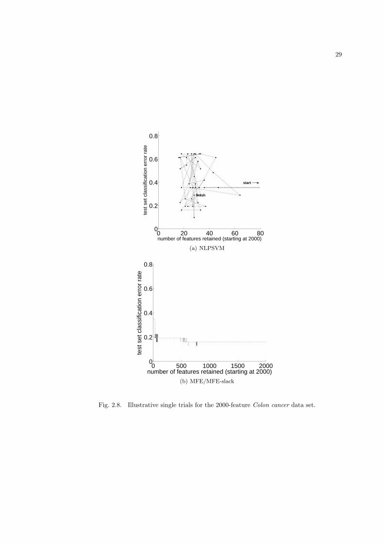
29

0 20 40 60 800

0.2

0.4

0.6

0.8


test

set

cla

ssifi

catio

n er

ror

rate

finish

start

(a) NLPSVM

0 500 1000 1500 20000

0.2

0.4

0.6

0.8


test

set

cla

ssifi

catio

n er

ror

rate

(b) MFE/MFE-slack

Fig. 2.8. Illustrative single trials for the 2000-feature Colon cancer data set.

30

than the MFE/MFE-slack test set error rate for these two data sets, and this is achieved with aslightly smaller number of selected features than MFE/MFE-slack.

2.4.5 Experiments on low-dimensional nonseparable data

For low-dimensional nonseparable data, average test set error rate curves are shown inFig. 2.10 for six (data set, kernel) pairings. Excluding Fig. 2.10(d), the curves in Fig. 2.10 (for5 data sets) are averages over 10, 10, 6, 6, 9 trials, respectively, which were the nonseparabletrials among the 10 trials generated. For Fig. 2.10(d), although the curves are averages over 9separable trials among the 10 trials generated, notice from the location of the vertical line thatwhile this UCI car data set was initially separable, it immediately lost separability when featureelimination commenced and thus we concluded it is more suitable for discussion in this sectionthan Sec. 2.4.4. The curves in Fig. 2.10 show that MFE-slack consistently achieved bettergeneralization performance than RFE and RFE-abs. Experiments (not shown) found this sameresult for additional (UCI data set, kernel) pairings. We also note that for flag and ionosphere inFig. 2.10 (and e.g. Fig. 2.6(a)), for which we applied RFE retraining, this retraining did improveperformance over RFE without retraining. In Figs. 2.10(a) and 2.10(b) (i.e. the linear kernelcase), the NLPSVM test set error rate (diamond) is slightly lower than the MFE/MFE-slack testset error rate (circle) albeit achieved with a slightly larger set of selected features.

2.4.6 High-dimensional feature space application: brain images

We processed 47 T1-weighted 3D MRI images (12 Alzheimer’s Disease (AD), 35 Control).After segmentation and registration, a Gray Matter tissue density image called “RAVENS”(17; 18; 35; 63) was generated for each by using the HAMMER software (62) and then smoothedby a 5mm Gaussian filter. After identically cropping all (3D) RAVENS images to remove non-brain background, we considered each voxel as a feature and performed SVM classification andfeature elimination experiments on a slice-by-slice basis, as follows. First, we split the 47 samplesinto a training set (X , with 8 AD and 25 Control samples) and a test set (X , with 4 AD and10 Control samples). For each of the (approximately) 150 2D (151×186) slices comprising a3D image, we trained a linear SVM, which perfectly classified all training samples as AD orControl. Next, the RFE and basic MFE methods each eliminated one voxel at a step, generatingeach method’s ordered set of discriminating voxels for that slice. Training set margins andtest set classification error rates were averaged over 55 (out of the 150) of these slice-specificclassifiers. Fig. 2.11 shows that MFE achieved larger margins and generalized better thanRFE. In Fig. 2.12, we show 12 slices that contain the hippocampus12, with a foreground ofoverlaid colors. The background image commonly used for such an overlay is the average overthe (spatially registered) brain image population used in the experiment – thus, in this case,it is the average of the RAVENS Gray Matter images. In Fig. 2.12(a), the orange regions arethose determined by MFE to be the most discriminating regions for AD, i.e. these contain theretained voxels for MFE up until the point where the data became nonseparable. Likewise,red indicates the regions found by RFE (with the same number of retained voxels as MFE),and white indicates the regions found by both MFE and RFE. Thus, Fig. 2.12(a) indicatesthat MFE is detecting the hippocampus, whereas RFE is not. Fig. 2.12(b) shows a confidenceranking among the MFE regions that were displayed (in orange and white) in Fig. 2.12(a).Higher rank for a voxel means it is more discriminating for AD. We indicate the ranking usingthe following colormap: red=high, yellow=higher, white=highest. The ranking was based simplyon the feature elimination order. Notice almost all of the smallest clusters (among the retainedvoxels which are shown in color) have received the lowest ranking – it is significant that MFE’smost discriminating voxels are found in sizeable, spatially compact voxel clusters. It is also

12A well-published “marker” brain structure for AD.

31

0 5 10 150

0.05

0.1

0.15

0.2


test

set

cla

ssifi

catio

n er

ror

rate


(a) UCI dermatology data set with 130 fea-tures; linear kernel

0 5 10 15 200

0.1

0.2

0.3

0.4

0.5

number of features retained (starting at 19)te

st s

et c

lass

ifica

tion

erro

r ra

te


(b) UCI hepatitis data set with 19 features; linearkernel

0 50 100 150 200 2500

0.05

0.1

0.15

0.2

0.25

0.3

0.35

0.4

0.45

0.5


test

set

cla

ssifi

catio

n er

ror

rate

RFEMFE/MFE−slackMFE−slackMFE−LO−FullMFE−LO−Lite

(c) UCI mfeat data set with 216 features; poly-nomial kernel

0 50 100 150 200 2500

2000

4000

6000

8000

10000

12000


mar

gin

RFEMFE/MFE−slackMFE−LO−FullMFE−LO−Lite

(d) UCI mfeat data set 216 features; polyno-mial kernel; margin

Fig. 2.9. Average test set classification error rate, (a)-(c), for three separable low-dimensionalUC Irvine data sets (Sec. 2.4.4). We truncated the dermatology graph from the right to zoom inon the most useful detail (see truncation description in Fig. 2.6). The vertical line indicates theaverage number of retained features at which separability was lost. Average training set marginis shown for one of the data sets in (d). Initial number of features is stated on the x-axis.

32

0 10 20 30 40 50 60 700

0.05

0.1

0.15

0.2

0.25

0.3

0.35

0.4

0.45


test

set

cla

ssifi

catio

n er

ror

rate

RFERFE−Retrain−LiteMFE−slackNLPSVM resultMFE−slack result

(a) UCI flag data set with 66 features; linearkernel

0 5 10 15 20 25 30 350

0.1

0.2

0.3

0.4

0.5

0.6


test

set

cla

ssifi

catio

n er

ror

rate

RFERFE−Retrain−LiteMFE−slackNLPSVM resultMFE−slack result

(b) UCI ionosphere data set with 34 features;linear kernel

0 50 100 150 200 250 3000

0.1

0.2

0.3

0.4

0.5


test

set

cla

ssifi

catio

n er

ror

rate

RFEMFE−slack

(c) UCI arrhythmia data set with 279 features;polynomial kernel

0 5 10 15 20 250

0.05

0.1

0.15

0.2

0.25

0.3


test

set

cla

ssifi

catio

n er

ror

rate

RFEMFE−slack

(d) UCI car data set with 21 features; polyno-mial kernel

0 20 40 60 800

0.1

0.2

0.3

0.4

0.5


test

set

cla

ssifi

catio

n er

ror

rate

RFERFE−absMFE−slack

(e) UCI cylinder data set with 78 features;Gaussian kernel

0 5 10 15 20 25 300

0.05

0.1

0.15

0.2

0.25

0.3

0.35


test

set

cla

ssifi

catio

n er

ror

rate

RFEMFE−slack

(f) UCI wisconsin-diagnosis data set with 29features; polynomial kernel

Fig. 2.10. Average test set classification error rate on 6 low-dimensional UC Irvine data sets(Sec. 2.4.5). Initial number of features is stated on the x-axis.

33

significant that, among the retained voxels, those in the hippocampus have almost uniformlyreceived the “higher”-to-“highest” ranking.

0 0.5 1 1.5 2 2.5 3x 104

0

5

10

15

20

25

30

35

40

number of features retained

mar

gin

RFEMFE

0 0.5 1 1.5 2 2.5 3x 104

0.25

0.3

0.35

0.4

0.45

0.5

0.55

0.6


clas

sific

atio

n er

ror

rate

RFEMFE

Fig. 2.11. Feature elimination results for high-dimensional brain image data, for the linear SVMcase. The initial number of features is 28,086.

2.5 Conclusions

In this chapter, we presented margin-based feature elimination and several extensions,applicable to SVMs and other linear and nonlinear, kernel-based discriminant functions. In thenonlinear kernel case, we identified shortcomings of RFE and demonstrated improved marginand accuracy achieved by kernel-based MFE. A second extension performs a lightweight SVMtraining that adjusts the current solution in the reduced feature space to improve margin. Ina third approach, MFE-slack, we formulated a simple extension of MFE to incorporate marginslackness. We evaluated on UCI data sets and gene microarray data sets, toward a comprehensiveevaluation of the generalization performances of MFE, RFE, and NLPSVM. We demonstratedthat MFE and MFE-slack provide better generalization than RFE, and better or competitivegeneralization compared with NLPSVM. We found that basic MFE, which requires separabledata, was always suitable for high-dimensional data but was also applicable for several low-dimensional UC Irvine data sets. We observed that methods which provide further increases inmargin beyond that of basic MFE did not necessarily lead to improved generalization. This wasattributed to overfitting and is consistent with the good performance achieved by MFE-slack,which introduces margin slackness. Finally, we also gave illustrative results on brain image data.

34

(a)

(b)

Fig. 2.12. Retained voxels (i.e. discriminating regions) for Alzheimer’s Disease in color (Sec.2.4.6).

35

Chapter 3

Margin-maximizing feature selection methods:

“multiclass” case (k > 2)

3.1 Introduction

Prior works introduced SVMs for the case of more than two classes (aka the “multiclass”case) – we begin this chapter by giving a summary of multiclass SVMs in Sec. 3.2. In Sec. 3.3we give an overview of RFE-based feature elimination methods for multiclass SVMs (77), wherewe discuss that these methods have been derived from the suboptimal two-class RFE objectiveand are thus again suboptimal, motivating us to develop multiclass “basic MFE”, i.e. MFE-k,starting with Sec. 3.4. We introduce several MFE-k methods, corresponding to several waysone can define “multiclass margin”, and for each method we again introduce a natural extensionthat incorporates slackness. Lastly in this chapter, in Sec. 3.7, we experimentally evaluate therelative performance of our multiclass MFE-based methods and show that MFE-k outperformsthe multiclass RFE-based methods.

3.2 Brief summary of multiclass SVMs

Consider a labeled training set (xn, pn), n ∈ Ω ≡ 1, . . . , N, where xn = [xn,1, . . . , xn,M ]T ∈RM is the n-th data sample and pn ∈ P ≡ 1, . . . , k is its class label. Denote p ≡ P\p. Let

Np be the number of samples in class p ∈ P , so N =K∑

p=1Np. Ωp ≡ n ∈ Ω|pn = p denotes

the set of samples in class p; Ωp,q ≡ Ωp ∪ Ωq. A multiclass support vector machine (SVM) isa linear or generalized linear classifier that achieves maximum margin, i.e. it maximizes theminimum distance of any training sample to the decision boundary. SVM training learns the setof discriminant functions fp(·), with the decision function given by:

p∗ = arg maxp∈P

fp(x). (3.1)

The “support vectors”, used to specify the SVM solution, are a special subset of the trainingpoints, identified below. Denote gn,q ≡ gq(xn) ≡ fpn

(xn) − fq(xn) for q ∈ pn, and Np,q ≡min

n∈Ωp,q

gn,rnwhere rn ≡ p, q\pn. Denote Ap ≡ l ∈ Ωp|gl,t > 0 ∀t ∈ p, the set of correctly

classified samples in class p, and A ≡k⋃

p=1Ap.

In the linear case, fp(x) ≡ wTpx + bp = 0, wp = [wp,1, . . . , wp,M ]T ∈ RM , bp ∈ R, p ∈ P .

Denote Lp,q ≡ ||wp−wq||2, dn,q ≡ gn,q√Lpn,q

(distance from sample xn to the class-pairwise decision

boundary between classes pn and q), and the class-pairwise margin γp,q ≡ γq,p ≡ minn∈Ωp,q

dn,rn,

rn = p, q\pn. For a sample xn, denote cn ≡ arg minq∈pn

dn,q, interpreted as follows: if xn is a

correctly classified sample, cn is the class to which xn is closest to being misclassified; else, ifxn is a misclassified sample, considering all (class-pairwise) boundaries between class pn and

36

another class o that xn is on the o side of (due to being a misclassified sample), cn is the classfrom which xn is furthest. In the linear case, gn,q = xT

n(wpn

− wq) + (bpn− bq) clearly, and

the weight vectors of the SVM solution are wp ≡∑

n∈Ω

Λn,p xn, where Λn,p ≡ (ζn,pAn − λn,p),

0 ≤ λn,p ≤ C are scalar Lagrange multipliers, An ≡k∑

p=1λn,p, and ζn,p is 1 if pn = p or is 0

otherwise (74). In the generalized linear (nonlinear) case, fp(x) ≡ wTpφ(x) + bp = 0, wp ∈ RL,

bp ∈ R, φ(x) ≡ [φ1(x), φ2(x), . . . , φL(x)]T, with φi(x) nonlinear functions of the x coordinates.Of particular interest is when inner products between φ(x) and φ(u) can be efficiently computedvia a positive definite kernel function, K(x, u) ≡ φT(x)φ(u). In this case, both φ(·) and wp itself(for any p ∈ P ) need not be explicitly defined since the SVM discriminant function fp(·) and theSVM weight vector squared 2-norm ||wp||2 can be expressed solely in terms of the kernel, i.e.:

fp(x) =∑

l∈Ω

Λl,pK(xl, x) + bp (3.2)

||wp||2 =∑

n∈Ω

∑

l∈Ω

Λn,pΛl,pK(xn, xl) (3.3)

Thus, gn,q and Lp,q are also expressed solely in terms of the kernel, i.e.:

gn,q = (∑

l∈Ω

Λl,pnK(xl, xn) + bpn

)− (∑

l∈Ω

Λl,qK(xl, xn) + bq) (3.4)

Lp,q ≡ ||wp−wq||2 ≡ ||wp||2+||wq||2−2wTpwq =

∑

n∈Ω

∑

l∈Ω

(Λn,pΛl,p+Λn,qΛl,q−2Λn,pΛl,q)K(xn, xl)

(3.5)This approach (the “kernel trick”), where K(·, ·) is chosen and applied within the SVM training,is referred to as the “nonlinear kernel case”.

Several distinct multiclass SVM training methods, each learning a multiclass discriminantof the form (3.1), have been proposed in prior works, e.g., (74), (70), (40), (36), (13). Of particularinterest is the Weston and Watkins (WW) method (74) which uses an “all-together” design,wherein discriminant functions for all classes are jointly learned to solve the single optimizationproblem given below by (3.6) (70; 74).

minw1,...,wk,b1,...,bk,ξ

12

k∑p=1

||wp||2 + C

N∑n=1

∑q∈pn

ξn,q s.t. ξn,q ≥ 0, gn,q ≥ 2− ξn,q, n = 1, . . . , N, q ∈ pn

(3.6)Recall that gn,q in the constraints in (3.6) (as well as in the constraints in (3.7) below) simplystands for xT

n(wpn

− wq) + (bpn− bq) in the linear case and 〈φ(xn), (wpn

− wq)〉 + (bpn− bq) in

the nonlinear kernel case – that is, as (3.6) states the training problem conveniently for bothcases, it is important to keep in mind that “w” (i.e. wpn

and wq) and “b” (i.e. bpnand bq)

indeed appear in the constraints. The design (3.6) allows slackness in the margin constraints, inparticular allowing both margin violations (i.e., ξn,q > 0) and misclassifications (a classificationerror occurs for sample n if ξn,q > 2 for any q ∈ pn).

The BSVM (biased SVM) training method (40), solving the problem given below in (3.7),

minw1,...,wk,b1,...,bk,ξ

12

k∑p=1

(||wp||2+b2p)+C

N∑n=1

∑q∈pn

ξn,q s.t. ξn,q ≥ 0, gn,q ≥ 2−ξn,q, n = 1, . . . , N, q ∈ pn

(3.7)

37

adds a bias term of b2p

to ||wp||2 in the WW objective function in (3.6). Adding the bias term inthe objective function was proposed by Mangasarian for the two-class case (26; 50) who showedthat the original and the modified SVM training problems differ only slightly (27; 50). Adding thebias term simplifies the corresponding dual problem and makes it faster to solve via decomposition(26; 77), and solutions of the modified formulation mostly coincides with solutions of the originalformulation (26). Since BSVM differs only slightly from WW, we use BSVM for training of theinitial multiclass classifier in our experiments, as implemented by the BSVM2 tool in the STPRtoolkit (65). Moreover, as we will discuss in Sec. 3.6, in one of our multiclass MFE methods,MFE-k-Kesler, we utilize the equivalence that exists via Kesler construction (20) between aone-class SVM problem and the BSVM formulation (as opposed to the WW formulation).

For choosing the SVM training parameter C as well as other SVM hyperparameters inthe nonlinear kernel case, we apply the standard practice of using a (bootstrap-based) validationprocedure (20).

3.3 Multiclass RFE-based methods

Similar to two-class RFE’s feature elimination criteria (equations (2.1) and (2.3) for the

linear case and nonlinear case, respectively),k∑

p=1w2

p,mwas used by (77) as the ranking criterion

for multiclass RFE methods discussed therein. Based on this criterion, (77) introduced andevaluated the feature elimination method MSVM-RFE-WW wherein the wp ∀p ∈ P are obtainedusing WW (3.6).

3.4 Multiclass MFE methods

MFE performs margin-maximizing feature elimination (for linear and nonlinear kernel-based binary (two-class) discriminant functions), and MFE-slack is a natural extension of MFEfor incorporating slackness and eliminating under nonseparability that reduces to MFE for largeenough C when the training data are separable. Aiming to improve on the RFE-based multi-class methods (e.g. MSVM-RFE-WW), we propose margin-optimizing feature elimination formulticlass SVMs, i.e. MFE-k. To develop our multiclass MFE approaches, we start by notingthat a training sample xn is classified as p∗

nin (3.1) if and only if gn,q > 0 ∀q ∈ p∗

n. Thus,

in the event that the training correctly classifies all training samples, the distances dn,q for alltraining samples xn are positive for all q ∈ pn. Based on this observation, there are several waysto define multiclass margin. First, we can define multiclass margin as γG, the global minimumclass-pairwise margin γp,q across all class pairs (p, q ∈ p) (there are

(k2

)such pairs):

γG ≡ minp,q∈p

γp,q (3.8)

Alternatively, as a second way, multiclass margin can be defined as γSP , the sum of all class-pairwise margins γp,q:

γSP ≡k∑

p=1

∑q<p

γp,q (3.9)

Finally, multiclass margin can be defined as γSC , the sum of all k classwise (one-versus-rest)margins, with classwise margin γp for class p defined as γp ≡ min

q∈pγp,q:

γSC ≡k∑

p=1

γp (3.10)

38

For an example separable data with three classes, Fig. 3.1(a) illustrates the(32

)class-pairwise

margins γp,q and states the resulting γG, γSP , and γSC .For separable training data, we propose the margin-maximizing feature elimination meth-

ods MFE-k-G, MFE-k-SP, and MFE-k-SC, which eliminate to preserve the largest γG, γSP ,and γSC , respectively. These methods require dn,pn

for all training samples xn to remain posi-tive upon elimination, i.e., mi, the feature eliminated at step i, must ensure gi,mi

n,q> 01 for all

(n ∈ Ω, q ∈ pn) pairs, i.e., mi must belong to the candidate feature set S(i) =⋂

p∈P, q∈p

Sp,q(i)

where Sp,q(i) ≡ m 6∈ M | N i,mp,q

> 0. The pseudocode for these three methods differ onlyslightly and are given in Sec. 3.4.1. In Sec. 3.5, we propose natural extensions of these threemethods, that allow incorporating slackness and eliminating under nonseparability, which, in theevent the data are separable reduce, for large enough C, to these three respective methods.

3.4.1 Pseudocode for algorithms MFE-k-G, MFE-k-SP, and MFE-k-SC, for linearand nonlinear kernel-based multiclass SVMs

0. Preprocessing: Let M be the set of eliminated features, with M = ∅ initially. First runSVM training on the full space to find a multiclass discriminant function set fp(·), p =1, . . . , k that correctly classifies each training sample xn. As confirmation that the setyou found is correctly classifying each xn, note that all g−1,0

n,qvalues you compute below

in the next sentence (for all (n ∈ Ω, q ∈ pn) pairs) must be positive. If linear kernel case,

∀(n ∈ Ω, q ∈ pn), compute δmn,q

≡ xn,m(wpn,m−wq,m) ∀m, and g−1,0n,q

= (bpn−bq)+

M∑m=1

δmn,q

,

where i = −1 means before eliminating any features and m−1 = 0 is a dummy placeholderindex value; if nonlinear kernel case, compute g−1,0

n,q∀(n ∈ Ω, q ∈ pn) using (3.4). Compute

L−1,0p,q

= ||wp − wq||2 for all (p ∈ P, q ∈ p). Set i ← 0. At elimination step i, perform thefollowing operations:

1. For each m 6∈ M, using recursion, compute gi,mn,q

for all (n ∈ Ω, q ∈ pn) pairs: if linearkernel case, this computation is gi−1,mi−1

n,q− δm

n,q, where δm

n,qneed not be computed in this

step if stored during preprocessing (step 0); if nonlinear kernel case, compute gi,mn,q

usingrecursion on the kernel computation. Determine N i,m

p,q= min

n∈Ωp,q

gi,mn,rn

for all (p ∈ P, q ∈ p)

pairs. Determine Sp,q(i) = m 6∈ M | N i,mp,q

> 0 and the candidate feature set S(i) =⋂p∈P, q∈p

Sp,q(i). If S(i) is empty (the data is nonseparable) then stop.2

2. For m ∈ S(i) and each class pair (p, q < p), using recursion compute Li,mp,q

: if linear kernelcase, this computation is Li,m

p,q= Li−1,mi−1

p,q− (wp,m − wq,m)2; if nonlinear kernel case,

compute Li,mp,q

using recursion on the kernel computation. Compute γi,mp,q

=N i,m

p,qqLi,m

p,q

.

1qi,m ≡ quantity q at feature elimination step i upon elimination of feature m.

2The set S(i) consists of the features at step i that, if singly eliminated, will preserve class-pairwise

positive margins. Margin will only be evaluated for features in the set S(i).

39

3.1. If using MFE-k-G, determine feature mi = arg maxm∈S(i)

minp∈P,q<p

γi,mp,q

; else if using MFE-k-SP,

determine feature mi = arg maxm∈S(i)

k∑p=1

∑q<p

γi,mp,q

; else if using MFE-k-SC, determine feature

mi = arg maxm∈S(i)

k∑p=1

minq∈p

γi,mp,q

. Eliminate feature mi, i.e. M→M∪ mi.

3.2. Keep for the next iteration only the recursive quantities associated with the eliminatedfeature – they are gi,mi

n,q∀(n, q) and Li,mi

p,q∀(p, q < p) in the linear kernel case, whereas,

in the nonlinear kernel case, they are the quantities defined for the recursive kernel com-putation (e.g., Hi,mi

k,n∀(k, n), Ki,mi

k,n∀(k, n)).

3.3. i → i + 1 and go to step 1.

3.5 Multiclass MFE-slack: utilizing margin slackness

In MFE-slack for the two-class case, as developed in (3), for each candidate feature forelimination, m, we evaluated every (correctly classified) training sample xn as the potentialmargin-defining sample (dubbed “anchor” xna

) associated with this elimination, and we chosethe pair (mMFE−S , nMFE−S) to minimize (via discrete optimization) the same objective functionas used by the pre-elimination SVM training and meet its constraints, with quantities in theobjective and constraints, such as slackness ξ, evaluated post-feature-elimination. We showedthat, for large enough C (and assuming the data is separable), positive slackness values are not

tolerated and minimization of 12 ||w||2 + C

N∑n=1

ξn (i.e., 12 (1/margin)2 + C

N∑n=1

ξn, where margin

1/||w|| was set by the anchor via scaling by a ρ parameter) reduces to minimization of 1/margin.Thus, MFE-slack reduces to strict margin-maximizing elimination (MFE) as a special case forlarge enough C. In a corresponding fashion, in the multiclass case, based on any one of theabove three definitions of multiclass margin we can choose the discrete maximization objectivefunction as multiclass margin minus a (C-weighted) sum of slackness values. Similar to thetwo-class case, maximizing this objective yields a slackness-based extension of multiclass MFEthat reduces to one of our (respective) strict-margin-achieving multiclass MFE methods for largeenough C. We next develop these slackness-based MFE-k extensions in subsections 3.5.1, 3.5.2,3.5.3. We will again denote that qi,mc,na ≡ quantity q at elimination step i upon elimination ofcandidate feature mc when the candidate anchor is xna

.

3.5.1 MFE-k-SP-slack

Based on the γSP definition, we choose the discrete maximization objective function forMFE-k-SP-slack as:

γSP − C

k∑p=1

∑q<p

∑

n∈Ωp,q

ψn,rn=

k∑p=1

∑q<p

(γp,q − C∑

n∈Ωp,q

ψn,rn) (3.11)

where rn ≡ p, q\pn (cf. Sec. 3.2) and meet the following slackness constraints upon choosinga correctly classified (candidate) class-pairwise anchor nap,q

∈ Ap ∪ Aq for each class pair (p ∈P, q ∈ p):

dn,rn≥ dnap,q

,rnap,q

− ψn,rn∀n ∈ Ωp,q, ∀(p ∈ P, q ∈ p), rn ≡ p, q\pn, ψn,rn

≥ 0 (3.12)

40

with slackness ψn,rnfor n ∈ Ωp,q defined as max(0, dnap,q

,rnap,q

− dn,rn), where dnap,q

,rnap,q

(which is computed asgnap,q

,rnap,q

||wp−wq|| ) sets the (possibly violated) class-pairwise margin γp,q in(3.11). In this method, each class pair has its own anchor for a given candidate feature forelimination. Thus, there are

(k2

)anchors working collectively for each candidate, m. In the

three-class example illustrated by Fig. 3.1(d) for the scenario where two dimensions remain uponcandidate elimination of one of three features, the encircled samples 7, 3, and 15 represent oneparticular choice of

(32

)anchors working collectively. These anchors are setting the class-pairwise

margins marked as γ1,3, γ2,1, γ2,3 (indicated by solid lines), relative to which the class-pairwise(positive) slacknesses (indicated in matching color, using short dashed lines) are calculated. Allanchor-based computations will be specified in detail in Sec. 3.5.1.1 shortly. MFE-k-SP-slackselects the pair (mSP−slack, nSP−slack

ap,q, q < p) that, post-elimination, maximizes (3.11) over

all the discrete choices (m, nap,q, q < p). MFE-k-SP-slack reduces to margin-maximizing

(γSP -maximizing) elimination for large enough C (assuming the data is separable).

3.5.1.1 MFE-k-SP-slack algorithm pseudocode for linear and nonlinear kernel-basedSVMs

0. Same as step 0 in Sec. 3.4.1, except the set of discriminating functions need not be aseparating one.

1. Using the recursive computation descriptions in steps 1 and 2 in Sec. 3.4.1, compute Li,mp,q

for all (m 6∈ M, p ∈ P, q ∈ p), and compute gi,mn,q

and di,mn,q

=g

i,m

n,qqLi,m

p,q

for all (m 6∈ M, n ∈Ω, q ∈ pn). We consider any data point to be a valid candidate anchor for feature eliminationcandidate m if it is not misclassified under that elimination; for each (m 6∈ M, p ∈ P ) pair,determine Ai,m

p= l ∈ Ωp|gi,m

l,t> 0 ∀t ∈ p (the set of valid candidate anchors in class p)

and Ai,m =k⋃

p=1Ai,m

p.

2. For each (m 6∈ M, p ∈ P, q ∈ p, nap,q∈ Ai,m

p∪ Ai,m

q) 4-tuple, to ensure zero slackness for

the class-pairwise anchor nap,q(i.e., ψ

i,m,nap,qnap,q

,rnap,q

= 0) and to meet all the constraints in

(3.12), compute ψi,m,nap,qn,rn

= max(0, di,mnap,q

,rnap,q

− di,mn,rn

) ∀n ∈ Ωp,q.

3.1 Determine the outcome (mi, niap,q

, p = 1, . . . , k, q < p) of the discrete maximization shown

below in (3.13), and eliminate feature mi, i.e., M→M∪ mi.3

arg maxm∈M

k∑p=1

∑q<p

maxnap,q

∈Ai,mp

∪Ai,mq

(di,mnap,q

,rnap,q

− C∑

n∈Ωp,q

ψi,m,nap,qn,rn

) (3.13)


3The simple default way to choose C in (3.13) is to set it to the C value used for the pre-elimination

SVM training; however, a different C value may be chosen for (3.13), e.g. based on a cross-validationprocedure applied after eliminating a batch of features.

41

(a) Illustration of γG, γSP , and γSC .

(b) MFE-k-G-slack-s (c) MFE-k-G-slack-m (d) MFE-k-SP-slack

(e) MFE-k-SC-slack-s (f) MFE-k-SC-slack-m

Fig. 3.1. Illustration of MFE-k and MFE-k-slack methods.

42

3.5.2 MFE-k-G-slack

We now choose the discrete maximization objective function for the elimination methodMFE-k-G-slack as γG (from (3.8)) minus a (C-weighted) sum of slackness values. For eachtraining sample xn, define a single slackness value ψn based on the sample’s proximity to theclass-pairwise boundary between the sample’s class pn and class cn, or alternatively, we candefine multiple slackness values ψn,q based on the sample’s proximity to each of the class-pairwiseboundaries between the sample’s class pn and the k − 1 other classes q 6= pn. For the first ofthese two methods, MFE-k-G-slack-s, we choose the objective as:

γG − C∑

n∈Ω

ψn (3.14)

and meet the following slackness constraints upon choosing a single, correctly classified (candi-date) global anchor na ∈ A:

dn,cn≥ dna,cna

− ψn, ψn ≥ 0, ∀n ∈ Ω (3.15)

with slackness ψn defined as max(0, dna,cna− dn,cn

), where dna,cna(which is computed as

gna,cna

||wpna−wcna

|| ) sets the (possibly violated) multiclass margin γG in (3.14). In the three-class

example illustrated by Fig. 3.1(b) for the scenario where two dimensions remain upon candi-date elimination of one of three features, the encircled sample 7 represents a particular choicefor the (single) anchor, which sets γG (marked γ2,1), relative to which the (positive) slacknesses(indicated in matching color) are calculated. All anchor-based computations for this method willbe specified in detail, shortly. MFE-k-G-slack-s selects the pair (mG−slack−s, nG−slack−s

a) below

that, post-elimination, maximizes (3.14) over all the discrete choices (m,na). For the secondmethod, MFE-k-G-slack-m, we choose the objective as:

γG − C∑

n∈Ω

∑q∈pn

ψn,q (3.16)

and meet the following slackness constraints upon choosing the global anchor na ∈ A:

dn,q ≥ dna,cna− ψn,q, ψn,q ≥ 0, ∀n ∈ Ω, ∀q ∈ pn (3.17)

with slackness ψn,q defined as max(0, dna,cna− dn,q), where dna,cna

sets the (possibly violated)multiclass margin γG in (3.16). Notice in Fig. 3.1(c) (which is for illustrating MFE-k-G-slack-m)that this figure differs from the above-discussed Fig. 3.1(b) in that multiple (positive) slacknessesare calculated for a sample for use by the algorithm (such as ψ13,1 and ψ13,2 for sample 13). Allanchor-based computations for this method will be specified in detail in Sec. 3.5.2.2 shortly.MFE-k-G-slack-m selects the pair (mG−slack−m, nG−slack−m

a) that, post-elimination, maximizes

(3.16) over all the discrete choices (m,na). Notice that each of these two methods reduces tomargin-maximizing (γG-maximizing) elimination (i.e. MFE-k-G, Sec. 3.4) for large enough C(assuming the data is separable).

3.5.2.1 MFE-k-G-slack-s algorithm pseudocode for linear and nonlinear kernel-based SVMs

0-1. Same as steps 0-1 in Sec. 3.5.1.1.

43

2. For each (m 6∈ M, n ∈ Ω) pair, determine ci,mn

= arg minq∈pn

di,mn,q

. For each (m 6∈ M, na ∈Ai,m) pair, to ensure zero slackness for the global anchor na (i.e., ψi,m,na

na= 0) and to meet

all the constraints in (3.15), compute ψi,m,na

n= max(0, di,m

na,ci,mna

− di,mn,ci,m

n

) ∀n ∈ Ω.

3.1 Determine the outcome (mi, nia) of the discrete maximization shown below in (3.18), and

eliminate feature mi, i.e., M→M∪ mi.

arg maxm∈M

maxna∈Ai,m

(di,mna,ci,m

na

− C∑

n∈Ω

ψi,m,na

n) (3.18)


3.5.2.2 MFE-k-G-slack-m algorithm pseudocode for linear and nonlinear kernel-based SVMs

This only differs from the pseudocode in 3.5.2.1 in steps 2 and 3.1.

2. For each (m 6∈ M, na ∈ Ai,m) pair, determine ci,mna

= arg minq∈pna

di,mna,q

, and, to ensure zero

slackness for the anchor (i.e., ψi,m,na

na,ci,mna

= 0) and to meet all the constraints in (3.17) compute

ψi,m,na

n,q= max(0, di,m

na,ci,mna

− di,mn,q

) ∀n ∈ Ω ∀q ∈ pn.

3.1 Determine the outcome (mi, nia) of the discrete maximization shown below in (3.19), and

eliminate feature mi, i.e., M→M∪ mi.

arg maxm∈M

maxna∈Ai,m

(di,mna,ci,m

na

− C∑

n∈Ω

∑q∈pn

ψi,m,na

n,q) (3.19)

3.5.3 MFE-k-SC-slack

Next, choose the discrete maximization objective function for the elimination methodMFE-k-SC-slack as γSC minus a (C-weighted) sum of slackness values. For a given class p, foreach training sample xn in class p, we can define a single slackness value ψn only based on thesample’s proximity to the class-pairwise boundary between the sample’s class p and class cn (cf.Sec. 3.2), or alternatively, multiple slackness values ψn,q based on the sample’s proximity to eachof the class-pairwise boundaries between the sample’s class p and the k− 1 other classes q 6= pn.For either of these two methods, with each class having its own anchor for a given candidatefeature for elimination, note that there are k anchors working collectively for each candidate, m.For the first of the two methods, MFE-k-SC-slack-s, we choose the objective as:

γSC − C

k∑p=1

(∑

n∈Ωp

ψn,cn+

∑

n∈Ωp

ψn,p) =k∑

p=1

(γp − C(∑

n∈Ωp

ψn,cn+

∑

n∈Ωp

ψn,p)). (3.20)

Associated with this objective, we meet the following slackness constraints in choosing a correctlyclassified (candidate) classwise (p-versus-rest) anchor nap

∈ A for each class p ∈ P (note: nap

need not be in Ap): define znapfor the anchor as znap

≡ cnapif the anchor is in p, or znap

≡ p

otherwise.dn,cn

≥ dnap,znap

− ψn,cn∀p ∈ P, ∀n ∈ Ωp, ψn,cn

≥ 0 (3.21)

dn,p ≥ dnap,znap

− ψn,p ∀p ∈ P, ∀n ∈ Ωp, ψn,p ≥ 0 (3.22)

44

with slackness ψn,cnfor n ∈ Ωp defined as max(0, dnap

,znap

− dn,cn) and ψn,p for n ∈ Ωp defined

as max(0, dnap,znap

− dn,p), where dnap,znap

sets the (possibly violated) classwise (p-versus-rest)

margin γp in (3.20). In the three-class example illustrated by Fig. 3.1(e) for the scenario wheretwo dimensions remain upon candidate elimination of one of three features, the encircled samples4, 7, and 16 represent a particular choice for the three anchors working collectively, which set thethree classwise margins (marked γ1, γ2, γ3, respectively), relative to which the (positive) slack-nesses (indicated in matching color) are calculated – in this particular example there are no (pos-itive) slacknesses relative to γ3. All anchor-based computations for this method will be specifiedin detail in Sec. 3.5.3.1, shortly. MFE-k-SC-slack-s selects the pair (mSC−slack−s, nSC−slack−s

ap)

that, post-elimination, maximizes (3.20) over all the discrete choices (m, nap, p = 1, . . . , k).

For the second method, MFE-k-SC-slack-m, we choose the objective as:

γSC − C

k∑p=1

(∑

n∈Ωp

∑q∈p

ψn,q +∑

n∈Ωp

ψn,p), (3.23)

equivalent tok∑

p=1

(γp − C(∑

n∈Ωp

∑q∈p

ψn,q +∑

n∈Ωp

ψn,p)) (3.24)

and meet the following slackness constraints and (3.22) upon choosing the classwise (p-versus-rest) anchor nap

∈ A for each class p ∈ P (note: again, napneed not be in Ap):

dn,q ≥ dnap,znap

− ψn,q ∀p ∈ P, ∀n ∈ Ωp, ∀q ∈ p, ψn,q ≥ 0 (3.25)

with slackness ψn,q for n ∈ Ωp defined as max(0, dnap,znap

− dn,q), where dnap,znap

sets the

(possibly violated) classwise margin γp in (3.24). Notice in Fig. 3.1(f) (which is for illustratingMFE-k-SC-slack-m) that this figure differs from the above-discussed Fig. 3.1(e) in that multiple(positive) slacknesses are calculated for a sample for use by the algorithm (such as ψ13,1 and ψ13,2

for sample 13) – in order to not crowd the figure, classwise margin and associated slacknesses arebeing illustrated for class 3 only. All anchor-based computations for this method will be specifiedin detail in Sec. 3.5.3.2 shortly. MFE-k-SC-slack-m selects the pair (mSC−slack−m, nSC−slack−m

ap)

that, post-elimination, maximizes (3.24) over all the discrete choices (m, nap, p = 1, . . . , k).

Notice that each of these two methods reduces to margin-maximizing (γSC-maximizing) elimi-nation (i.e. MFE-k-SC, Sec. 3.4) for large enough C (assuming the data is separable).

3.5.3.1 MFE-k-SC-slack-s algorithm pseudocode for linear and nonlinear kernel-based SVMs

0-1. Same as steps 0-1 in Sec. 3.5.1.1.

2. For each (m 6∈ M, p ∈ P, n ∈ Ωp) triplet, determine ci,mn

= argminq∈p

di,mn,q

. For each (m 6∈M, p ∈ P, nap

∈ Ai,m) triplet: first, determine zi,mnap

(which is ci,mnap

if the anchor is in p or is p

otherwise); second, to ensure zero slackness for the anchor (i.e., ψi,m,nap

nap,zi,m

nap

= 0) and to meet

all the constraints in (3.21) and (3.22), compute ψi,m,napn,cn

= max(0, di,mnap

,zi,mnap

−di,mn,ci,m

n

) ∀n ∈

Ωp and ψi,m,napn,p

= max(0, di,mnap

,zi,mnap

− di,mn,p

) ∀n ∈ Ωp.

45

3.1 Determine the outcome (mi, niap

, p = 1, . . . , k) of the discrete maximization shown belowin (3.26), and eliminate feature mi, i.e., M→M∪ mi.

arg maxm∈M

k∑p=1

maxnap

∈Ai,m(di,m

nap,zi,m

nap

− C(∑

n∈Ωp

ψi,m,napn,cn

+∑

n∈Ωp

ψi,m,napn,p

)) (3.26)


3.5.3.2 MFE-k-SC-slack-m algorithm pseudocode for linear and nonlinear kernel-based SVMs

This only differs from the pseudocode in 3.5.3.1 in steps 2 and 3.1.

2. For each (m 6∈ M, p ∈ P, na ∈ Ai,m) triplet: first, determine zi,mnap

(which is ci,mnap

if

the anchor is in p or is p otherwise), and, to ensure zero slackness for the anchor (i.e.,

ψi,m,nap

nap,zi,m

nap

= 0) and to meet all the constraints in (3.25) and (3.22) compute ψi,m,napn,q

=

max(0, di,mnap

,zi,mnap

− di,mn,q

) ∀n ∈ Ωp ∀q ∈ p and ψi,m,napn,p

= max(0, di,mnap

,zi,mnap

− di,mn,p

) ∀n ∈ Ωp.

3.1 Determine the outcome (mi, niap

, p = 1, . . . , k) of the discrete maximization shown belowin (3.27), and eliminate feature mi, i.e., M→M∪ mi.

arg maxm∈M

k∑p=1

maxnap

∈Ai,m(di,m

nap,zi,m

nap

− C(∑

n∈Ωp

∑q∈p

ψi,m,napn,q

+∑

n∈Ωp

ψi,m,napn,p

)) (3.27)

3.6 MFE-k-Kesler

3.6.1 Kesler construction

The Kesler construction generates a set of higher-dimensional samples starting from thesamples of a multiclass classification problem (k > 2) so that the multiclass LDF problem canbe cast using a (higher-dimensioned) two-class LDF. We begin this section by stating the Keslerconstruction – additional description can be found in other sources, e.g. (20). For each originalM×1 sample xn, k−1 Kesler samples zn

q(with q ∈ pn) are constructed, each being a concatenation

of k vectors that are each (M + 1)-dimensional, with augmented vector an = [xTn

1]T the pn-th vector, −an the q-th vector, and each of the other k − 2 vectors given by an (M + 1)-dimensional vector of zeroes. The total number of Kesler samples is thus (k − 1)N . Denotezn

q≡ [zn

1,q, . . . , zn

k(M+1),q]T (also just denoted zn

q≡ [z1, . . . , zJ ]T with J ≡ k(M + 1)). For

example, if k = 3, for each xn in class 2 the following two (i.e. k−1) Kesler samples z2q, q ∈ 1, 3

are constructed: z21

= [−aTn

aTn

0T]T, z23

= [0T aTn− aT

n]T.

As previously shown by e.g. (20), (26), the Kesler construction can be used to express themulticlass problem as a one-class problem – in particular, form:

W = [W1, . . . , Wk(M+1)]T ≡ [ [wT

1, b1], . . . , [w

Tk, bk] ]T. (3.28)

Thus let us denote a discriminant function example by F (z) ≡ WTz. Note first that the con-straints in (3.7) are captured by WTzj ≥ 1 − ξj , j = 1, . . . , (k − 1)N . Second, note that||W ||2 =

∑p∈P

||wp||2 + b2p. Thus, it is easy to see that the multiclass SVM training problem in

46

(3.7) can be recast in terms of the augmented weight vector W and the Kesler samples via

minW,ξ

12||W ||2 + C

J∑

j=1

ξj s.t. ξj ≥ 0, F (zj) ≥ 1− ξj , j = 1, . . . , (k − 1)N. (3.29)

For a Kesler sample z, let Tm denote the Kesler feature subset m,m + (M + 1), . . . , m +(k−1)(M +1) with values determined by the original feature m – only two of these k are actualoccurrences of original feature m in any given Kesler sample, as the remaining k−2 are 0. Thus,denoting:

∆tn,q

≡ znt,q

Wt, q ∈ pn, 4 (3.30)

∆mn,q

≡∑

t∈Tm

∆tn,q

, q ∈ pn, (3.31)

it becomes obvious that∆m

n,q= δm

n,q, q ∈ pn. (3.32)

3.6.2 MFE-k-Kesler

The idea of our MFE-k-Kesler feature elimination method for the multiclass case is toconstruct Kesler samples z from the original samples x and utilize the equivalence between (3.7)and (3.29). Specifically, (3.29) is a one-class SVM problem (all Kesler samples on the same sideof the hyperplane W ). Accordingly, for feature elimination consistent with the optimization in(3.29), we apply two-class MFE (cf. Ch. 2, (3)) on the one-class nature of Kesler samples z,which is a valid approach because, the one-class problem is a two-class problem where all samples(the Kesler samples) are in class +1 (and none in class −1) and lie on a side (the same side) of ahyperplane (i.e. the Kesler hyperplane) W given by (3.28). At elimination step i, MFE-k-Keslereliminates the Kesler feature ti whose elimination yields the largest remaining (positive) Keslermargin (i.e. minimum distance from the Kesler samples to W ). After the elimination sequenceof Kesler features is obtained using this criterion, the elimination sequence of original features isobtained from it as follows. An original feature m is eliminated when all t ∈ Tm are eliminated– this generates a complete elimination sequence of original features.

3.7 Results

We performed experiments to compare our multiclass MFE-k methods with multiclassRFE-based methods. For experimental procedure for the initial classifier training, and exper-imental procedure for feature elimination, we followed the approach discussed earlier for thetwo-class case (cf. Sec. 2.4.1 and 2.4.2). Also as in the two-class case, to continue the elim-ination process after loss of separability, we define the “hybrid” MFE-k/MFE-k-slack methods(such as MFE-k-G/MFE-k-G-slack-m), where, simply, MFE-k (such as MFE-k-G) is used for thesteps where the data is separable (including the initial step) and the corresponding MFE-k-slackmethod (such as MFE-k-G-slack-m corresponding to MFE-k-G) is used for the other steps.

For the case of the linear kernel, test set classification error rate curves for our MFE-kmethods and the RFE-based MSVM-RFE-WW method are shown in Fig. 3.2 for two UC Irvinedata sets. All curves shown are averages over 10 trials – and for each trial, the initial SVM was atraining set separator. For our three MFE-k methods MFE-k-G, MFE-k-SP, and MFE-k-SC, weshow that the first two had a tie for best performance, under our “slack-m” approach for slackness

4The product on the RHS contains also a multiplication by yzn

q, not being shown as it is 1 ∀n.

47

(as opposed to the less rigorous “slack-s”) – notice in the figure that this is true for both thehybrid method (e.g. MFE-k-G/MFE-k-G-slack-m) and the solely slackness-based method (e.g.MFE-k-G-slack-m). We also show that our above three “basic MFE-k” methods achieved muchbetter generalization performance (lower test set error rate curve) than MSVM-RFE-WW. Ageneralization performance comparison between these MFE-k methods and MFE-k-Kesler is notavailable in this thesis and can be generated in future work – however, in Fig. 3.3(a), we showthat MFE-k-Kesler achieved much better generalization performance than MSVM-RFE-WW.

In conclusion, for feature elimination in the multiclass SVM case, our multiclass MFEmethods that we advocate are: MFE-k-G/MFE-k-G-slack-m, MFE-k-SP/MFE-k-SP-slack, aswell as MFE-k-Kesler. Our multiclass method that we advocate the most at this time is MFE-k-G/MFE-k-G-slack-m, because e.g. 1) it requires less computation than MFE-k-SP/MFE-k-SP-slack which had similar generalization performance, and 2) both the number of samples and thenumber of features are increased approximately k-fold when MFE-k-Kesler is used.

48

0 50 100 150 200 2500

0.1

0.2

0.3

0.4

0.5

0.6

0.7


test

set

cla

ssifi

catio

n er

ror

rate

MSVM−RFE−WWMFE−k−G/MFE−k−G−slack−sMFE−k−G/MFE−k−G−slack−mMFE−k−SC/MFE−k−SC−slack−sMFE−k−SC/MFE−k−SC−slack−mMFE−k−SP/MFE−k−SP−slackMFE−k−G−slack−sMFE−k−G−slack−mMFE−k−SC−slack−sMFE−k−SC−slack−mMFE−k−SP−slack

(a) UCI mfeat data set with 216 features; linear kernel

0 20 40 60 80 100 120 1400

0.1

0.2

0.3

0.4

0.5

0.6

0.7


test

set

cla

ssifi

catio

n er

ror

rate

MSVM−RFE−WWMFE−k−G/MFE−k−G−slack−sMFE−k−G/MFE−k−G−slack−mMFE−k−SC/MFE−k−SC−slack−sMFE−k−SC/MFE−k−SC−slack−mMFE−k−SP/MFE−k−SP−slackMFE−k−G−slack−sMFE−k−G−slack−mMFE−k−SC−slack−sMFE−k−SC−slack−mMFE−k−SP−slack

(b) UCI dermatology data set with 130 features; linear kernel

Fig. 3.2. Average test set classification error rate, (a)-(b), for two separable low-to-intermediatedimensional UC Irvine data sets (Sec. 3.7). Initial number of features is stated on the x-axis.

49

0 50 100 150 200 250 300

0.2

0.3

0.4

0.5

0.6

0.7

0.8

0.9


test

set

cla

ssifi

catio

n er

ror

rate

MSVM−RFE−WWMFE−k−Kesler

(a) UCI arrhythmia data set; linear kernel

Fig. 3.3. Average test set classification error rate for the UCI arrhythmia data set; linear kernel(Sec. 3.7).

50

Chapter 4

MRI brain image processing and

analysis of Alzheimer’s disease and its onset

Note for ADNI: The author, of this thesis chapter i.e. manuscript, is Yaman Aksu, forthe Alzheimer’s Disease Neuroimaging Initiative*.

*Data used in preparation of this article were obtained from the Alzheimer’s Disease Neu-roimaging Initiative (ADNI) database (http://www.loni.ucla.edu/ADNI). As such, the investiga-tors within the ADNI contributed to the design and implementation of ADNI and/or provideddata but did not participate in analysis or writing of this report. A complete listing of ADNIinvestigators can be found at:http://www.loni.ucla.edu/ADNI/Collaboration/ADNI Authorship list.pdfThe ADNI was launched in 2003 by the National Institute on Aging (NIA), the National In-stitute of Biomedical Imaging and Bioengineering (NIBIB), the Food and Drug Administration(FDA), private pharmaceutical companies and non-profit organizations, as a $60 million, 5-yearpublic-private partnership. The primary goal of ADNI has been to test whether serial magneticresonance imaging (MRI), positron emission tomography (PET), other biological markers, andclinical and neuropsychological assessment can be combined to measure the progression of mildcognitive impairment (MCI) and early Alzheimer’s disease (AD). Determination of sensitive andspecific markers of very early AD progression is intended to aid researchers and clinicians todevelop new treatments and monitor their effectiveness, as well as lessen the time and cost ofclinical trials. The Principal Investigator of this initiative is Michael W. Weiner, M.D., VAMedical Center and University of California - San Francisco. ADNI is the result of efforts ofmany co-investigators from a broad range of academic institutions and private corporations, andsubjects have been recruited from over 50 sites across the U.S. and Canada. The initial goal ofADNI was to recruit 800 adults, ages 55 to 90, to participate in the research – approximately200 cognitively normal older individuals to be followed for 3 years, 400 people with MCI to befollowed for 3 years, and 200 people with early AD to be followed for 2 years.

4.1 Introduction

The dementing illness Alzheimer’s disease (AD), and the state of transition between nor-mal aging and AD referred to as mild cognitive impairment (MCI), continue to be widely studied.MCI includes people with memory impairment without meeting dementia criteria. Annually anestimated 10-15% of people with MCI are diagnosed with AD (54). Moreover, even prior toclinical symptoms, larger increases in structural brain abnormality have been found in peoplewith MCI compared to normal (“Control group”) people, via retroactive evaluation of serial(longitudinal) MRI scans (16). Furthermore, AD diagnosis is not considered definitive withoutconfirming AD-characteristic pathologies such as the debated amyloid deposits detectable at au-topsy. Motivated by reasons such as the above, there has been much recent analysis of both ADand MCI, to better understand the disease onset and progression to aid diagnosis and effectivetreatment development. A substantial aim is to develop methods with promising clinical value,which include 1) methods that can effectively aid diagnosis only based on a single (first) visit forthe person, 2) methods that can effectively predict which MCI individuals are likely to convert,

51

especially imminently, to AD, and 3) methods for treatment monitoring. Such methods can bedriven by seeking “biomarkers” – these include feature selection methods, as discussed in Ch. 1.Alternatively, methods may attempt to diagnose without seeking biomarkers – these include theuse of SVM classification based on the full feature set (without feature selection). In Ch. 4, weexperiment with both of these approaches, using SVMs and MFE.

For all aims mentioned above, structural MRI analysis may prove useful as it addressesmany complexities of AD and MCI such as the following. First, even at an early, clinicallynormal stage of AD or MCI, brain atrophy may exhibit complex patterns spatially distributedto many brain regions (10; 23; 25) – due to cell loss there may be cortical thinning (47; 66) andventricle dilation and gaping (11; 59), volumetric and shape changes in the hippocampus andentorhinal cortex (15; 19; 64), temporal lobe shrinkage (58), and other morphological changes.Second, since atrophy patterns may be more subtle at the early disease stage (11; 16; 25) and maychange during disease progression, quantifying patterns early is a big challenge. Third, patternsattributable to normal aging are a confounding factor in the search for patterns that characterizedisease (57).

Consider a population of AD/MCI/Control brain MR 3d images segmented into numerous(e.g. 100) intricate regions defined by a brain anatomy atlas – such images would enable numer-ous region-specific volumetric measurements, useful towards detecting brain atrophy typical forAD/MCI subjects. A second useful image type would be 3d “volumetric density” images – onefor gray matter and one for white matter – where, this time we are referring to an image typethat both 1) has been considerably registered across the population (i.e. “spatial normalization”into a single spatial frame of reference) and 2) has voxel values that represent how much “localvolume” for the corresponding tissue (e.g. gray matter) in the original (pre-registration) multi-tissue image had to be dilated or contracted by the registration to fit into that density imagevoxel. A possible advantage of such density images over the region-segmented image is the muchlarger number of volumetric measurements (i.e., one per voxel) that it provides per brain. Inthis thesis we are using the HAMMER registration method and software tool for generating suchtissue density images – a separate density image is generated for each of three “tissues” (graymatter, white matter, ventricles), and as mentioned above the voxel values of this set of threeimages by definition sum to the pre-registration brain volume. Typically, including the case ofthis thesis, populations of such image types (e.g. region-segmented, or density) are not commonlyreadily available and instead only the original images, which were generated by the MR scanneritself (e.g. T1-weighted images), are available as image populations. In this thesis we use HAM-MER for generating both of the above two useful image types – we elaborate on this methodand tool in Appendix C. Sec. 4.2 discusses our image processing pipeline that includes also non-HAMMER components that are necessary for generating some types of intermediate images fromthe original (T1-weighted) MR images, including “tissue-segmented” images. Tissue-segmentedimages, which are a required HAMMER input, are images that consist of the following segments:gray matter, white matter, ventricles, (non-ventricle) cerebrospinal fluid (CSF), (non-anatomy)background.

As noted by a number of prior works e.g. (11), statistical and predictive power, andvalidity, of an AD analysis method producing spatio-temporal “patterns” of brain regions, areof much interest. In the domain of AD analysis using MRI, a number of prior works utilizedpattern recognition – those that utilized SVM classifiers in particular, as we do in this chapter,include (16; 51; 71). These particular prior studies are significantly notable also because, inorder to capture interactions among effects in regions throughout the brain, without making apriori assumptions about specific regions to be measured, each of these methods jointly analyzedvoxels (or regions) spanning the entire brain, whereas a number of other studies have focused onspecific regions of interest (ROIs), especially the regions mentioned above such as hippocampusand ventricles.

52

The data used in the experiments in this chapter were obtained from the ADNI database(2), for which three “ground-truth” clinical labels, assigned by clinicians, were available: AD,MCI, Control. This label may be derived from multiple criteria, including CDR (Clinical De-mentia Rating) whose possible values are: 0=none, 0.5=questionable, 1=mild, 2=moderate,3=severe. ADNI aims to recruit and follow 800 research participants in the 55-90 age range:approximately 200 elderly people to serve as Controls (Normal Controls), 400 people with MCI,and 200 people with AD. The “ground-truth” label (AD, MCI, or Control) was assigned in ADNIat first visit – however, at a later visit there is no stated conversion from one ground-truth labelto another, and thus, for example we do not know if or when (at which visit) a participant whois non-AD at first visit converts to AD. On the other hand, available to us are visit-specificnumerical data, including structural MR (T1-weighted) images and non-image data such as CDRscore and age, enabling cross-sectional analysis (across a population) and/or longitudinal analysis(across time).

In prior work on AD analysis with MRI data e.g. (51), for some classification experiments,the MCI population was broken up into two subpopulations (classes), according to whether, overtime, an MCI participant’s CDR score of 0.5 stayed the same or increased. Herein we refer to thissubgrouping approach as the “conversion-by-CDR” approach1. The concept of conversion-by-CDR should be considered with great caution because there is very significant AD-MCI overlapwith respect to the CDR value of 1 and even 0.5 – more specifically, considering the ADNIdatabase as an example (an example with a very large subject population), the majority of thehundreds of AD participants start (at first visit) at 0.5 and stay at 0.5 at the later visits, whileat the same time all (or almost all) of the hundreds of MCI participants start at 0.5, with thevast majority of these MCIs staying at 0.5 at the later visits. Very relevant to this overlap issue,a significant contribution of this thesis is our following novel approach for detecting (possible)conversion to AD, driven by image-based information, rather than by a single, non-image-basedmeasurement such as CDR. Upon building a Control-AD classifier (using only AD and Controlsubjects), we use it to classify all available longitudinal 3d images2 of the training MCI subjects,so as to utilize their distances to this single Control-AD boundary from one visit to the next. Anexample illustration of these person-specific trajectories of longitudinal phenotype scores (positivefor Control-like and negative for AD-like) is given by Fig. 4.1(a) – phenotype score vs. age isplotted, with each set of connected dots being a separate person. People who are converters-by-CDR are shown in different color than people who are nonconverters-by-CDR. Also, solely forclearer viewing, the subject population is further broken up in Fig. 4.1(a) into a top and bottomgraph, with the top showing people whose score was less for final visit than first visit, and viceversa for the bottom graph – notice that there are many more people who become more AD-likethan Control-like over time. As illustrated by Fig. 4.1(b), we then fit a line (using least-squares)on a person-by-person basis. Consider the following four fitted-score (fs) categories:

1. fs starts and ends positive.

2. fs starts and ends negative.

3. fs starts positive and ends negative.

1While this term says “conversion”, note that it does not mean an actual conversion to AD which

requires assignment of the participant by a clinician to the AD label at the later visit – recall thatinformation is not available. We will refer to the two classes formed by the conversion-by-CDR approachas “converters-by-CDR (cc)” and “nonconverters-by-CDR (ncc)”, e.g. the “MCIcc” and “MCIncc”classes.

2Here we are simply saying “image” to refer to our particular feature set for the image which is not

necessarily a set of voxel values, e.g. some experiments in this chapter use volumes of brain regions asfeatures.

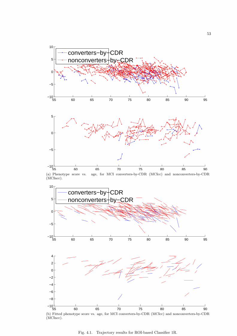
53

55 60 65 70 75 80 85 90 95−10

−5

0

5

10

55 60 65 70 75 80 85 90−10

−5

0

5

converters−by−CDRnonconverters−by−CDR

(a) Phenotype score vs. age, for MCI converters-by-CDR (MCIcc) and nonconverters-by-CDR(MCIncc).

55 60 65 70 75 80 85 90 95−10

−5

0

5

10

55 60 65 70 75 80 85 90−10

−8

−6

−4

−2

0

2

4


(b) Fitted phenotype score vs. age, for MCI converters-by-CDR (MCIcc) and nonconverters-by-CDR(MCIncc).

Fig. 4.1. Trajectory results for ROI-based Classifier 1R.

54

4. fs starts negative and ends positive.

For all types of features in our experiments herein, we consistently found that at least 90− 95%of our training MCI population fell into the first three of the above four fs categories. Since thesethree represent almost the entirety of the MCI population, we can legitimately define categories2 and 3 together as “the first of two classes of MCI subjects” and category 1 as “the second of thetwo classes of MCI subjects”, based on which we can then build a new type of two-class classifier.More specifically, since subjects in category 1 are more Control-like than AD-like throughout theirvisits, we can declare they define (belong to) a “nonconverters-by-trajectory’ (MCInct) class, andlikewise, since subjects in category 2 and 3 are more AD-like than Control-like by the time oftheir final visit, we declare they define (belong to) a “converters-by-trajectory” (MCIct) class.3

Note, very importantly, that when building this new classifier, each training sample would comefrom the first visit alone, not from multiple visits. We shall refer to this approach as “conversion-by-trajectory” – clearly, its strength is two-fold:

1. Previously unseen (test) patients would be classified (diagnosed) based on their first visitalone, i.e. this is an early diagnosis approach.4

2. Unlike in the conversion-by-CDR approach, the two MCI subpopulations involved are beingdefined using image-based information, without using CDR. This is an advantage because,first, a rise in a person’s CDR from 0.5 to 1, utilized by the above alternative conversion-by-CDR approach, may not be a strong indicator on which to define MCI subpopulations,and second, assigned CDR values and their change over time may be considerably noisy.

Note that the legitimacy of the conversion-by-trajectory approach stems from the fact that thetest MCI subjects are not being used when building either of the above two in-tandem classi-fiers. We will show experimentally that the conversion-by-trajectory approach outperforms theconversion-by-CDR approach.

A second major novel aspect, and significant contribution, of the AD/MCI analysis inthis thesis is that MFE is used as the feature selection method, whereas prior works (16; 51)(mentioned above) utilized RFE which was shown in this thesis (Ch. 2) to be consistentlyoutperformed by MFE in a comprehensive evaluation, i.e. for both separable and nonseparabledata, for a variety of data set examples for both linear and kernel-based classification.

A third notable aspect for this thesis is that the experiments are utilizing a much largerpopulation of ADNI subjects and their longitudinal images (≈ 2000 images in total) than wehave seen in prior works.

Sec. 4.2 discusses our image processing pipeline. Sec. 4.3 discusses our extensive setof experiments and gives experimental results and comparisons. Sec. 4.4 gives the chapterconclusions.

4.2 Brain MR image processing pipeline

For the image processing pipeline used by this thesis, let us begin by giving a shortoverview of the pipeline steps. The input (3d) image is a T1-weighted MR image of the head.As first step, this image is coarsely aligned with a reference atlas (aka Atlas1) using rigid-body

3Since category 2 by definition starts and ends more AD-like than Control-like, there is no “conversion”

taking place for it per se, but we do include this category together with category 3 in our convenientlynamed “converters”-by-trajectory class because they end AD-like just as category 3 does.

4As a reminder, note that the person to be diagnosed must be excluded from the population used

to construct (train) the classifier(s) to be used for the diagnosis – this is a pattern classification designrequirement.

55

registration, whereby the AC (Anterior Commisure) landmark in the brain also becomes placedat the origin. Then, non-brain anatomy is removed from the aligned head images. The resultingbrain-only 3d image is tissue-segmented into the five segments required by HAMMER: whitematter (WM), gray matter (GM), ventricles, (non-ventricle) CSF, (non-anatomy) background.Lastly, a second atlas (aka Atlas2, an atlas by MNI (Montreal Neurological Institute) distributedwith HAMMER), serving as the reference atlas to be used by HAMMER registration, is inputinto HAMMER along with the five-segment image, to generate the above-mentioned density3d image (RAVENS map) and the 3d region-segmented image – a separate RAVENS map isgenerated for each of three “tissues”: GM, WM, ventricles. The sum of voxel values across thesethree RAVENS images (cf. Sec. 4.1) is on the order of 106 and varies across people – to removeperson-specific brain volume as a bias, the set of three RAVENS images is normalized such thateach person would have the same volume. As elaborated at the end of this section, the normalizedRAVENS images are then smoothed spatially using a 5mm FWHM Gaussian filter.

For Atlas1, we used the MNI/ICBM (International Consortium for Brain Mapping) atlas,resampled to 1mm isotropic voxel dimensions. The alignment to Atlas1 is performed using FSL’slinear image registration tool FLIRT (41). The subsequent non-brain removal is performedusing FSL’s brain extraction tool BET (60). The subsequent tissue-segmentation step consistsof three substeps. The first substep is the commonly used approach of tissue segmentationinto four (of the above-mentioned five) segments, with ventricles and CSF together labeled asCSF. This segmentation is performed using FSL FAST (76). The second substep is the useof the labelVN tool in HAMMER for (automatically) segmenting CSF into ventricles and (non-ventricle) CSF. The third and final substep is to process the resulting five-segment 3d image withour fv (fill ventricles) algorithm whose purpose is to automatically remedy the problem wherethe above ventricle segmentation by HAMMER (which is a deformation process for matching tothe ventricles of Atlas2) is often incomplete as a consequence of a subject’s anatomy being toodifferent from the atlas. This problem is a common scenario as AD/MCI patients often have veryenlarged and distorted ventricles due to atrophy. We describe fv in Appendix A.2 – its underlyingassumption is that the ventricles that HAMMER does find, which we viewed in numerous brains,are reliable despite being incomplete.5

HAMMER generates the RAVENS maps by performing a deformation between the sub-ject’s tissue-segmented (five-segment, 3d) image and the corresponding tissue-segmented (five-segment, 3d) Atlas2 image6. Also available in the Atlas2 image set is the already region-segmented version of this atlas with approximately 100 anatomical regions. This availability is amain reason we are using this particular atlas - using this atlas (i.e., both its region-segmentedand five-segment versions) and HAMMER, the pipeline is able to produce a region-segmentedimage from an individual’s five-segment image.

In our above pipeline steps used in this thesis, as a matter of fact the use of the MNI/ICBMatlas (for the initial linear registration), our fv algorithm, and the RAVENS normalization andsmoothing are the only steps that were not included in our original pipeline which was developedand delivered by us to PSU Hershey CNMRR in 2006 and 2007 which gave rise to our collabora-tion with Dr. D. Bigler at CNMRR for co-developing a pipeline improved with new capabilitiesnamed STAMPS (7) which is discussed in Appendix A.3 – notice in the Appendix that several ofthe types of output images that STAMPS can readily generate are not used by this thesis. For ourabove-mentioned pipeline steps in this thesis, we created and used a new and customized version

5A known HAMMER property is that it conservatively adjusts the amount of deformation depending

on the task so as to control the amount of noise in the result.6Since the region-segmented atlas distributed with HAMMER (Atlas2) had much better segmentation

quality than the tissue-segmented (five-segment) atlas distributed with HAMMER (Atlas2), the formerwas used, by Dr. D. Bigler, to create a replacement for the latter by simply forming region unions. Thetissue-segmented Atlas2 that we used was this replacement image.

56

of STAMP/STAMPS, which we shall simply refer to as “STAMPY/STAMPYS”. The differencesbetween STAMPS and STAMPYS can be understood via comparing our above description ofour processing steps with STAMPS steps described in (7). In understanding these differences,it is also important to understand that STAMPYS stemmed from the fact that STAMPS hasseveral major limitations. We have met these critical challenges – note some example differencesbetween STAMPS and STAMPYS described below:

1. STAMPS’ interface to the cluster (i.e., supercomputer), described in (7), is both complexand assumes that the user has much system administration control, at will, over how thejob processes are to be distributed to the cluster nodes. This approach was designed by ourpipeline collaborator Dr. D. Bigler specifically with the PSU Hershey CNMRR cluster inmind, and overrode the interface approach of our above-mentioned pre-STAMPS pipelinewhich is simple so as to make it functional on the PSU UP HPC clusters (on which wedo not have system administration control). The UP HPC clusters, together providing atleast ten times the processing power of the CNMRR cluster alone, have been essential toour work because, as anticipated, it has been necessary to process more than a thousandADNI 3d images – not just a single time but rather at will, with each image taking severalhours to process. Here, a big challenge was the need to process this many images and todo so in a timely manner (again, not once but as many times as the need arises). Whilemore than a thousand samples is of course not necessary for a classification experiment,processing 1000 − 2000 images with the pipeline has been necessary, as follows. As Sec.4.3 will demonstrate concretely, the actual number of samples per class that 1000 − 2000images provide us can often be as low as 100, or even 50, because the thousand is a unionthat accounts for i) three subject categories (AD, MCI, Control), ii) up-to-6 visits (i.e.up-to-6 images) per subject7, and iii) a wide age range whereas we often require 1-to-1age-matching (cf. Sec. 4.3.3) across classes in our classification experiments herein for ADanalysis.

2. As stated in (7), a hard-coded STAMPS step that precedes the rigid-body registrationthresholds the input T1-weighted image. While (7) essentially suggests this hard-codedstep is innocuous so long as T1-weighted images have sufficient signal-to-noise ratio, wehave discovered that this step often destroys ventricle voxels by setting them to 0, causingsubsequent pipeline images (such as the region-segmented image and the RAVENS ventriclemap) to be incorrectly generated. Thus, in our pipeline in this thesis (STAMPY), thethresholding step is removed.

3. While (7) essentially declares that STAMPS has a functioning FSL-based segmentationoption apart from its SPM/VBM-based segmentation option, as it turned out FSL-basedsegmentation was actually not fully implemented into STAMPS even though it was in-deed implemented into our original pre-STAMPS pipeline. As we discussed above (Sec.4.2), STAMPYS implements and uses FSL-based segmentation – this is mainly becauseSPM/VBM segmentation in the STAMPS design (or a third segmentation option differentfrom SPM/VBM and FSL) was not made feasible on the PSU UP HPC clusters. The in-feasibility was due to the fact that it was required in STAMPS to assign the segmentationtask to distributed Matlab computing despite the incompatibility of this approach withthe restrictions in the UP HPC configuration, such as HPC’s dmatlab (restrictive, custom,front-end component for controlling distributed Matlab computing) and HPC’s particularmethod of distributing Matlab licenses.

7Sec. 4.3 will describe that our diagnosis procedure utilizes training data from up-to-6 visits (i.e.

up-to-6 images) per subject (rather than relying on a simpler classification experiment procedure) so asto aim for sufficient specificity and sensitivity towards diagnosis.

57

4. The automated pipeline STAMPYS contains our abovementioned fv tool which enablesit to remedy the abovementioned ventricle segmentation problem in an automated way,whereas the automated pipeline STAMPS does not contain a similar (automated) tool, asmentioned by footnote 6 in (7). This is a very significant limitation in STAMPS when theimage population that needs to be processed is large.

We now elaborate on the RAVENS smoothing mentioned above. The focus of RAVENSis to preserve volume on a tissue-by-tissue basis through the registration process. When creatingRAVENS, HAMMER relaxes the amount of warping to combat noise inherent in the nonlinearregistration so as to properly detect (and encode) brain atrophy. Consequently, there is consid-erable inter-person variability in RAVENS images, which is commonly mitigated by smoothingthe RAVENS (or the normalized RAVENS) images. Since RAVENS smoothing is not yet madea part of the pipeline (in STAMPS or STAMPYS), we performed the smoothing afterwards, inan automated way.

4.3 Results

4.3.1 ADNI data

Herein we only use “processed” images present in the ADNI database, i.e. images thathave undergone ADNI’s image correction which is described at the ADNI website.8 The numberof Control, MCI, and AD participants used in our analysis were approximately 180, 300, and 120,respectively. For each Control we used, we only used the participant’s initial visit with CDR=0– the reason is that after the initial visit approximately 10% of these Control participants haveCDR=0.5 (just as some MCI and even AD participants do) and thus, these non-initial visits forControls, if used, would have introduced a confounding effect into the analysis which we chooseto simply avoid in this particular case since 180 Control images is sufficient. For MCI and ADparticipants, from the discussion in Sec. 4.1 on our methods it should be clear that we usedmultiple visits.

4.3.2 ROI-based and voxel-based experiments

We performed two types of experiments: ROI-based (R) and voxel-based (V). In the Rcase, the features are 101 normalized region volumes obtained from the region-segmented images,wherein a region’s volume is normalized by dividing it by the total volume of all regions. In theV case, which is much higher dimensional with more than 20,000 features, the features are thevoxel intensities of a smoothed RAVENS map. As a reminder from Sec. 4.1, while each ofthese two types of features is volumetric information, V may produce, as this thesis will explore,more accurate generalization due to both the number and finer granularity of its volumetricmeasurements (i.e., one feature per voxel) that it provides per brain. For both experiment types,we will build several SVM classifiers (named Classifier 1, Classifier 2, etc.) that differ solely byclass design (i.e., how the particular population for the classifier is constructed or defined) – wewill refer to the ROI-based and voxel-based instances of Classifier 1 as Classifier 1R and Classifier1V, respectively. For the V case only, we will additionally perform a statistical paired t-test forcomparison, using the same sample set as the SVM classifier we are comparing it with.

8See www.loni.ucla.edu/ADNI/Data/ADNI Data.shtml. ADNI image correction steps include Grad-

warp, N3, and scaling for gradient drift. As suggested by the above ADNI website, we sought image fileshaving “N3” and “scaled” in the file name.

58

4.3.3 Procedure for initial classifier training for AD/MCI/Control data

For AD/MCI/Control data, for training of the initial SVM classifier (i.e., the classifier priorto potentially subsequently applying feature selection on it), we used the experimental procedurespecified below – notice that fundamentally it is an extension of our standard procedure (Sec.2.4.1) so as to incorporate new aspects appropriate for this data, such as the treatment of age asa confounding variable. For a given participant, image data may be available for multiple visits– however, note that the procedure is restrictive in that every “sample” (exemplar) input fortraining the SVM classifier shall not combine data from multiple visits (for a given participant)– consequently each sample does only have a single age associated with it. Also note that theprocedure does ensure that a given participant contributes a sample (or samples) to either thetraining set or the test set but not both – there is a set of training participants, from which theset of training images (samples) are obtained, and likewise there is a set of test participants, fromwhich the set of test images (samples) are obtained.

Let Pc be the set of participants in class c ∈ C ≡ 1, . . . , k where k is the number ofclasses.9

Step 1. Prepare training set and test set: For each c ∈ C, Pc is randomly split 90%-10%into a non-heldout (training) set Pc,nh and a heldout (test) set Pc,h.

Step 2 (optional). Age-match: As per the single-age-per-sample restriction stated above, weproduce subsets Pc,nh,a ⊂ Pc,nh ∀c ∈ C such that each sample in Pc,nh,a is “age-matched”(i.e. age-separated by no more than one whole year) to a unique sample in each of the other(i.e. C\c) classes. Establishing this tight age correspondence between classes in the trainingset contributes to mitigating the confounding effect of age (with a second contributor beingour “adjust feature values for age” step discussed below), as well as makes the trainingdata readily suitable for a statistical paired t-test (with which we compare our methods).Upon matching, to utilize any non-matched (leftover) samples of the non-heldout set, wemove them to the heldout set. Subsequently, as in Ch. 2 (and in (3)), let X and X denotethe non-heldout (training) and heldout (test) set of samples (as opposed to participants)respectively.

Step 3. Remove constant features: Features constant across the non-heldout samples (inX) are removed from all (non-heldout and heldout) samples.

Step 4. Adjust feature values for age: This step uses a basic approach that aims to removethe confounding effect of age from the data, prior to classification. For each feature m,first, model the feature value as a function of age a by computing the least-squares-fit linelm(a) ≡ α1a + α2 through the points (ai, xi,m) where the index i traverses the non-heldoutsamples, and for ith such sample (with age ai) the value of feature m is xi,m. Next, usingthis line (i.e., α1 and α2 computed for feature m), for each (heldout or non-heldout) sampleadjust xj,m (with j denoting the sample index) by subtracting lm(aj) ≡ α1aj + α2.

Step 5. Normalize: For each feature m, compute the minimum value minnh and themaximum value maxnh for the feature across non-heldout samples, and normalize thefeature’s value vj for every (heldout and non-heldout) sample j by setting it to (vj −minnh)/(maxnh−minnh). This normalizes the non-heldout set’s feature values to the [0,1]range, and the heldout set’s feature values to the [0,1] range.

Step 6. Train a classifier as described by Steps 2-4 of our “Experimental Procedure for theInitial Classifier Training” in Ch. 2 (and in (3)).

9While we are stating the procedure for suitability with any number of classes, note that set C is

±1 for our experiments herein.

59

4.3.4 Classifier 1: Control-AD123 classifier

Using the “initial classifier training procedure” (cf. Sec. 4.3.3), we build the Control-ADclassifier discussed in Sec. 4.1, herein referred to as Classifier 1, using only a single, CDR=0image for Control subjects and all available CDR≥ 1 images for “AD123” subjects (who are, bydefinition, the AD subjects with at least one visit having a CDR of 1, 2, or 3). Note that ADsubjects who start and stay at CDR=0.5, and thus are perhaps too MCI-like throughout theirvisits, are excluded from this Control-AD classifier. Recall from Sec. 4.3.2 that we will referto distinct classifiers “Classifier 1R” and “Classifier 1V”, corresponding to the ROI-based andvoxel-based cases for Classifier 1 respectively.

Since all MCI participants in our analyses herein have a CDR of 0.5 at initial visit, oneinteresting question for early diagnosis of AD is as follows.

Q1: Using (classifying) an MCI participant’s initial visit alone, how well does Classifier 1predict whether this MCI participant will experience a rise in CDR (i.e. a “conversion-by-CDR”,suggesting possible conversion to AD)? In our experiments below, this is one of the questions wewill address.

4.3.4.1 Classifier 1R: features are ROI-based

Several results are shown for Classifier 1R in Table 4.1. With the test set being somewhatclass-balanced with respect to the number of samples (76 Controls, 57 ADs), and the two class-specific test set misclassification rates being close to each other (0.07 for Controls, 0.12 for ADs),in this particular experiment the overall test set misclassification rate is a fairly good indicatorfor this entire test population – note that this rate (0.09) is low, and thus we can say Classifier 1Rperforms quite well and confidently proceed to characterizing our MCI data with this classifierthroughout this chapter.

Note that answering Q1, for Classifier 1R, involves a special classification – an AD-Controlclassifier that was trained without using people with MCI is used to classify people with MCI.Accordingly, for this special classifier, we can define “misprediction” intuitively as an MCInccperson classified as AD or an MCIcc person classified as Control. Then, for Classifier 1R, theanswer to Q1 is: not well at all. Table 4.1 states that the “misprediction” rate for 252 MCIparticipants (209 MCIncc, 43 MCIcc) is high (0.36), and thus a better early diagnosis system isneeded than 1R alone.

Since 1R gave high accuracy for Control and AD data, we now highlight the brain regionsthat MFE selected based on this classifier. Listed under 1R in Table 4.1, the circle on the MFEtest set error graph indicates that ten out of 101 brain regions were selected using MFE, listedabove the graph (in order of elimination). Entorhinal cortex and hippocampus, which are well-published biomarkers for AD, were found by MFE to be the 4th and 5th most discriminating forthe disease among the 101 brain regions. As in Ch. 2 (and (3)), the graphs show MFE performedwell: the MFE/MFE-slack test set error curve trend is again flat; a large percentage of features iseliminated without a big change in classification accuracy relative to the initial (pre-elimination)classifier; and MFE again outperformed RFE.

4.3.4.2 Classifier 1V: features are voxel-based

Recall that the features used by our voxel-based SVM classifiers herein, including thisfirst voxel-based classifier named Classifier 1V, are the voxel intensities of the three types ofsmoothed and subsampled RAVENS maps (GM, WM, ventricles). For such classifiers, we createdthe RAVENS subsample via skipping five RAVENS voxels along each of the three axes – asdescribed in Appendix B.0.1, with the (I, J,K) associated with skips of five being equal to(6, 6, 6), each RAVENS map is exhaustively broken up into 216 subsamples. In conjunctionwith the exhaustive subsampling approach, in Appendix B.0.1 we introduced the “hierarchical

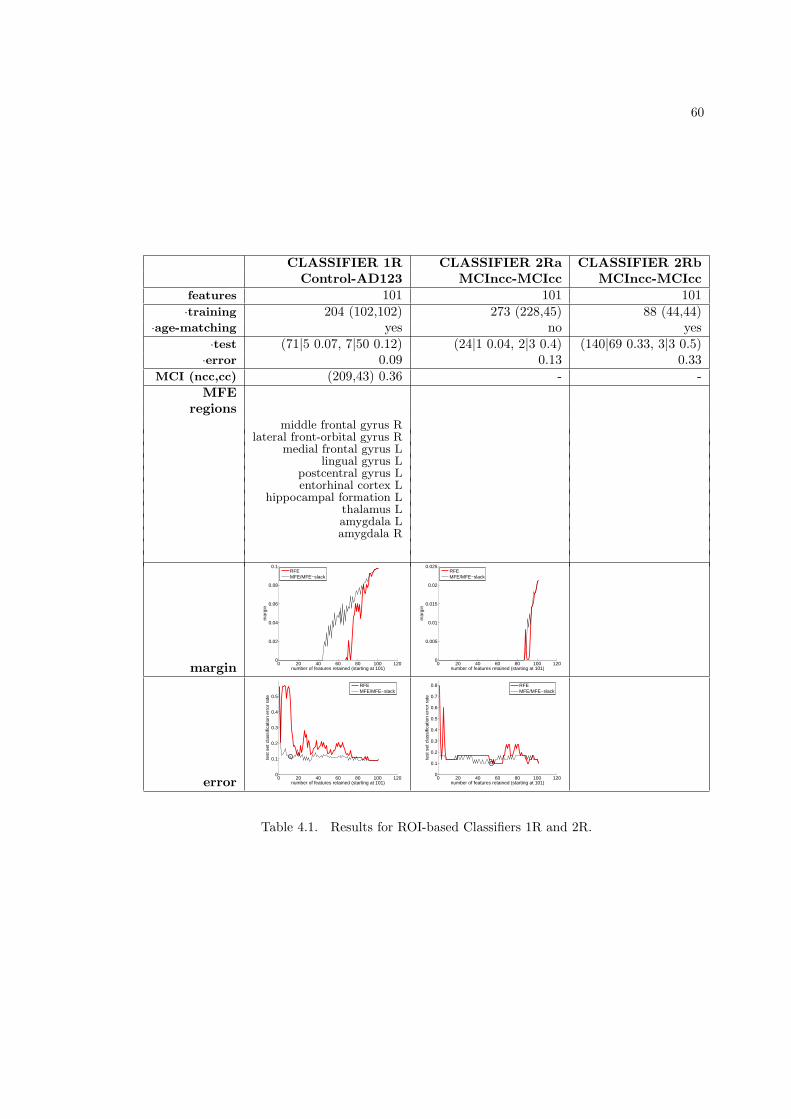
60

CLASSIFIER 1R CLASSIFIER 2Ra CLASSIFIER 2RbControl-AD123 MCIncc-MCIcc MCIncc-MCIcc

features 101 101 101·training 204 (102,102) 273 (228,45) 88 (44,44)

·age-matching yes no yes·test (71|5 0.07, 7|50 0.12) (24|1 0.04, 2|3 0.4) (140|69 0.33, 3|3 0.5)·error 0.09 0.13 0.33

MCI (ncc,cc) (209,43) 0.36 - -MFE

regionsmiddle frontal gyrus R

lateral front-orbital gyrus Rmedial frontal gyrus L

lingual gyrus Lpostcentral gyrus Lentorhinal cortex L

hippocampal formation Lthalamus Lamygdala Lamygdala R

margin 0 20 40 60 80 100 1200

0.02

0.04

0.06

0.08

0.1


mar

gin

RFEMFE/MFE−slack

0 20 40 60 80 100 1200

0.005

0.01

0.015

0.02

0.025


mar

gin

RFEMFE/MFE−slack

error 0 20 40 60 80 100 1200

0.1

0.2

0.3

0.4

0.5


test

set

cla

ssifi

catio

n er

ror

rate

RFEMFE/MFE−slack

0 20 40 60 80 100 1200

0.1

0.2

0.3

0.4

0.5

0.6

0.7

0.8


test

set

cla

ssifi

catio

n er

ror

rate

RFEMFE/MFE−slack

Table 4.1. Results for ROI-based Classifiers 1R and 2R.

61

MFE (H-MFE)” feature elimination procedure that is simply a series of steps where each stepsimply re-groups multiple feature subsets provided by the previous step (and then applies MFEon each resulting group), with the initial step’s feature subsets being the subsamples’ individualMFE-selected feature sets. However, herein we do not give results for H-MFE, i.e. the Classifier1V results we will discuss are only based on a single one subsample among the 216. Several1V results are shown in Table 4.2. First, the test set misclassification rate (0.08) of the initial(pre-elimination) classifier is low, and very close to the rate found above for the ROI-based case(0.09, cf. Sec. 4.3.4.1), and thus, as in the ROI-based case we are able to confidently proceedto characterizing our MCI data with this Control-AD classifier (1V) throughout this chapter.Second, the graphs (Table 4.2) show MFE again performed well: the MFE/MFE-slack test seterror curve trend is again flat; a large percentage of features is eliminated without a big drop fromthe accuracy of the initial classifier. In addition, a slow drop in training set margin during MFEis observed. Third, Fig. 4.2 shows the brain regions selected by MFE (i.e. regions discriminatingbetween AD and Control).

CLASSIFIER 1VControl-AD123

features 21,633·training 144 (72,72)

·age-matching yes·test (105|4 0.04, 7|20 0.26)·error 0.08

MCI (ncc,cc) (168|62 0.27, 27|22 0.55) 0.32

margin 0 0.5 1 1.5 2 2.5

x 104

0

0.5

1

1.5

2

2.5

3

3.5


mar

gin

MFE/MFE−slack

error 0 0.5 1 1.5 2 2.5

x 104

0

0.1

0.2

0.3

0.4

0.5

0.6

0.7

0.8


test

set

cla

ssifi

catio

n er

ror

rate

MFE/MFE−slack

Table 4.2. Results for voxel-based Classifier 1V.

Next, we built Classifier 1Vb whose results are shown in Table 4.3. Classifier 1Vb differsfrom Classifier 1V in that 1Vb only used the gray matter RAVENS image and a single subsampleamong a total of eight (resulting in 84,627 features) whereas 1V had used all three RAVENS im-ages and a single subsample among a total of 216 (resulting in 21,633 features). As shown by the1Vb results in Table 4.3, in this particular experiment instance the use of a smaller subsamplingfactor (producing a larger number of features) did not lower the test set misclassification rate.

62

Fig. 4.2. Regions found by MFE with Classifier 1V.

CLASSIFIER 1VbControl-AD123


·age-matching yes·test (108|1, 10|17)·error 0.08

Table 4.3. Results for voxel-based Classifier 1Vb.

63

55 60 65 70 75 80 85 90−2

−1.5

−1

−0.5

0

0.5

1

1.5

55 60 65 70 75 80 85 90 95−1.5

−1

−0.5

0

0.5

1

1.5


(a) Phenotype score vs. age, for MCI converters-by-CDR (MCIcc) and nonconverters-by-CDR(MCIncc).

55 60 65 70 75 80 85 90−2

−1.5

−1

−0.5

0

0.5

1

1.5

55 60 65 70 75 80 85 90 95−1.5

−1

−0.5

0

0.5

1

1.5


(b) Fitted phenotype score vs. age, for MCI converters-by-CDR (MCIcc) and nonconverters-by-CDR(MCIncc).

Fig. 4.3. Trajectory results for voxel-based Classifier 1V.

64

4.3.5 Classifier 2: MCIncc-MCIcc (nonconverters-by-CDR vs. converters-by-CDR)

Sec. 4.3.4 showed that Classifier 1 alone is not sufficient for predicting (possible) conversionfrom MCI to AD in the conversion-by-CDR sense using an MCI participant’s initial visit alone.However, recall that Classifier 1 did give high accuracy (91% for ROI-based, 92% for voxel-based) for Control and AD data, and thus the poor prediction performance of Sec. 4.3.4 forMCI resulting from CDR-driven categorization is attributable to: a) the CDR values being noisyand/or b) a switch for an MCI participant from 0.5 to 1 obviously not necessarily meaning anactual conversion from MCI to AD. Recall that in fact half of all participants clinically labeled asAD at initial visit have a CDR of 0.5 at that visit, just as all MCI participants do at their initialvisit, which, again, stresses the inherent complexity of the AD/MCI/Control classification (anddiagnosis) problem. Consequently, to more closely investigate the classification problem for MCIparticipants in particular, and the role of CDR for that task, as well as to evaluate our MFEmethod for this particular case, first we built an MCI-specific classifier using the conversion-by-CDR approach (cf. 4.1 of prior works such as (16; 51; 71), which we refer to as Classifier 2 –recall that this classifier is a stand-alone classifier not built in-tandem with results from anotherclassifier such as Classifier 1. After evaluating Classifier 2 in this section, in the next sectionwe will build Classifier 3, our novel classifier which, unlike Classifier 2, is built in-tandem withClassifier 1 so as to utilize the concept of conversion-by-trajectory.


As shown in Table 4.1, Classifiers 2Ra and 2Rb were built, without and with age-matchingrespectively. With age-matching, notice from the figure that the training set for 2Rb is class-balanced but only 44 training subjects per class were available (which is less than half the numberused for Classifier 1R), whereas, without age-matching for 2Ra the number of available class 1subjects (MCI “nonconverters-by-CDR”) rises to 228 – notice from the figure that the trainingset for 2Ra is thus very class-imbalanced. Test misclassification rate was quite high for both ofthese classifiers – for Classifier 2Rb it was high for both classes, whereas in 2Ra it was high onlyfor class 2 (MCI “converters-by-CDR”). Since the features used in Classifier 2R are the same onesused in Classifier 1R which did give high accuracy in that case (for Control and AD participants),the fundamental weakness of Classifier 2R is perhaps not the quality of the features but ratherthat Classifier 2R is driven by an MCI categorization based on CDR measurements which maybe noisy. To address these open questions, and the fact that these results show that Classifier2R alone, just like Classifier 1R alone, is not sufficient for predicting conversion from MCI toAD using an MCI participant’s initial visit alone, we are motivated to proceed to our above-mentioned diagnosis approach wherein, again, we will use Classifier 1R to obtain trajectories tobe used to build Classifier 3R (which will thus serve in-tandem with Classifier 1R).

4.3.6 Classifier 3: MCInct-MCIct (nonconverters-by-trajectory vs. converters-by-trajectory)

We would like to only use a single visit for a test MCI individual in order to diagnosewhether or not the individual will convert to AD. Note that this aim is very closely related toQuestion 1. Based on Sec. 4.1, our procedure for this particular type of diagnosis is as follows:

Step 1. Build Classifier 1 using the procedure in Sec. 4.3.3.

Step 2. Generate two MCI subgroups: Use Classifier 1 to calculate a phenotype score foreach of the available longitudinal images of the population of training MCI subjects, andbreak up this population into the MCIct and MCInct subgroups as described by Sec. 4.1.

Step 3. Build Classifier 3: Again using the training procedure of Sec. 4.3.3, build theMCInct-MCIct classifier, herein referred to as Classifier 3.

65

Step 4. To diagnose a test individual, classify him/her using Classifier 3. If he/she isclassified as MCIct, the diagnosis is that he/she will convert to AD; otherwise the diagnosisis that he/she will not convert to AD.

Although this particular diagnosis procedure is clearly suitable for MCI individuals, let us nowdiscuss whether it is also suitable for any individual. For people with AD and healthy people,clearly all that the procedure can really declare is whether the person is (a) more like MCI peoplewho will convert to AD or (b) more like MCI people who will not convert to AD. Therefore, clearlyit is not a complete procedure for declaring whether a person will convert to AD (or has AD).However, the procedure is useful for also a healthy (non-MCI) person because clearly one shouldcertainly expect almost all healthy people to be classified as MCInct rather than MCIct. On theother hand, it is not reasonable to expect almost all people with AD to be classified as MCIct bythis procedure. One reason is, as discussed in Sec. 4.1 a very large percentage of all AD and MCIsubjects (half of all AD and big majority of all MCI) do exhibit similar characteristics over timesuch as a non-varying CDR of 0.5 over time. Nevertheless, in Sec. 4.3.6.1 and Sec. 4.3.6.2 wewill evaluate the above diagnosis procedure for people with AD (in addition to MCI and healthypeople).

Note again that the above diagnosis procedure essentially serves to predict whether aperson will be AD in the future. To diagnose whether a person has AD at present, recall thatClassifier 1 can be used but it is, again, by design clearly more reliable for people with AD andhealthy people than people with MCI. For an improved diagnosis procedure to address this issue,an additional component can be introduced into our above diagnosis procedure. The componentwould employ a new classifier, which would be similar to Classifier 3 in that it would be based onthe trajectories, but dissimilar in that this time it would produce the two MCI subgroups basedon a new criterion that takes into account also the trajectories of the training individuals withAD. The new procedure’s AD diagnosis can then be combined with the AD diagnosis of Classifier1 (which classifies an individual as Control or AD) – for this, basic voting or a more sophisticatedensemble learning approach can be employed. Alternatively, more than two subgroups can beproduced, to then build a multiclass classifier.


Notice from Table 4.4 that we have built Classifiers 3Rc and 3Rd to correspond to Classi-fiers 2Ra and 2Rb we discussed above in Sec. 4.3.5, using the same features – that is, notice thatClassifier 3Rd was trained under age-matching using 44 samples per class (just as in Classifier2Rb), and Classifier 3Rc due to no age-matching was trained with several times as many class 1samples as the 45 class 2 samples (just as in Classifier 2Ra). Comparing test set misclassificationrates on a class-by-class basis, we see that Classifier 3Rd’s rates were 0.28 for class 1 and 0.29for class 2, whereas the rates of its counterpart Classifier 2Rb were much higher: 0.33 for class1 and 0.5 for class 2. Similarly comparing Classifier 3Rc to 2Ra, we see that the rates 0.08 and0.25 of Classifier 3Rc are overall better than the rates of 0.04 and 0.4 of Classifier 2Ra. Thuswe can perhaps conclude that our novel in-tandem classification approach, involving two classi-fiers (1R and 3R), has successfully introduced an improvement towards solving the problem ofpredicting conversion from MCI to AD using an MCI participant’s initial visit alone. In fact, tosee that the magnitude of the improvement is perhaps bigger than implied by the above ratesalone, let us now consider our Classifiers 3Ra and 3Rb also shown in Table 4.4. These twoclassifiers, with larger training set sizes than 3Rc and 3Rd, were generated for our in-tandemclassification procedure – more specifically: 1) to obtain the 44 age-matched sample pairs with

66

which to build 3Rd, we simply omitted 54 of the 98 age-matched pairs of 3Rb (cf. Table 4.4)10,and 2) to obtain the 118 class 1 samples and the 45 class 2 samples with which to build 3Rc,we simply took all 118 class 1 samples of 3Ra (cf. Table 4.4) and omitted 99 of the 144 class 2samples of 3Ra (cf. Table 4.4). With that said, notice in Table 4.4 that our approach is able toachieve a test classification accuracy of 80%. (51) reported this same number for their methods– this is a remarkable comparison between their methods and our method because their methodis actually based on a more sophisticated pre-classification image preparation procedure whereinspecial features are extracted from RAVENS maps. In other words, while our features may beless powerful, the above-demonstrated strength of our novel in-tandem classification procedure isone way we are overcoming that limitation. Moreover, additionally using MFE, we may achievefurther improvements – for example, the test set error graphs for both our Classifiers 3a and 3bshow that the error rate drops below 0.2 under MFE/MFE-slack elimination.

In Table 4.4, the “test Control” row indicates that the big majority of Control subjectswere consistently classified as MCInct rather than MCIct, as anticipated by the above discussionin Sec. 4.3.6. The “test AD123” row indicates that the big majority of AD123 subjects wereconsistently classified as MCIct rather than MCInct – an expected result because recall thatthese particular AD subjects have high CDR throughout their visits. Within the group of ADsubjects who had a CDR of 0.5 at first visit, the majority was classified the same as the ADsabove who had come in with a high CDR (i.e. the majority was classified as the MCI class thatis eventually on the AD side of the Control-AD boundary). Within this group of AD subjects,some had gone to a higher CDR at a subsequent visit (i.e. the “test ADcc” row) whereas othershad stayed at 0.5 (i.e. the “test ADncc” row). Those with a subsequently high CDR resembled,at first visit, those who had started with a high CDR more than did those who stayed at 0.5,with respect to the above classification. In one experimental example (Classifier 3Ra) consideringthose who had stayed at 0.5, while 72% were classified as the converting MCI class (a relativelysmall number, perhaps due to it being difficult to discriminate between ADs and MCIs stayingat 0.5), the percentage is higher for AD subjects who either start at a high CDR (e.g. 94%) oreventually increase to a high CDR (e.g. 77%).

10After sorting the 98 age-matched sample pairs by age, first we omitted every other pair and then we

omitted 5 additional pairs so that 44 pairs would remain, so as to maintain the uniformity of the agedistribution of the remaining pairs.

67

CLA

SSIF

IER

3Ra

CLA

SSIF

IER

3Rb

CLA

SSIF

IER

3Rc

CLA

SSIF

IER

3Rd

MC

Inct

-MC

Ict

MC

Inct

-MC

Ict

MC

Inct

-MC

Ict

MC

Inct

-MC

Ict

featu

res

101

101

101

101

·train

ing

262

(118

,144

)19

6(9

8,98

)16

3(1

18,4

5)88

(44,

44)

·age-m

atc

hin

gno

yes

noye

s·te

st(9|4

0.3,

2|14

0.13

)(1

0|30.

23,4|1

20.

25)

(12|1

0.08

,4|1

20.

25)

(48|1

90.

28,20|50

0.29

)·er

ror

0.2

0.24

0.17

0.28

test

AD

ncc

11|29

11|29

18|22

15|25

test

AD

123

1|15

2|14

3|13

3|13

test

AD

cc

3|10

4|96|7

4|9te

stC

ontr

ol

59|17

61|15

68|8

62|14

mar

gin

020

4060

8010

012

00

0.00

5

0.01

0.01

5

0.02

0.02

5

0.03

0.03

5

num

ber

of fe

atur

es r

etai

ned

(sta

rtin

g at

101

)

margin

RF

EM

FE

/MF

E−

slac

k

020

4060

8010

012

00

0.01

0.02

0.03

0.04

0.05

0.06

num

ber

of fe

atur

es r

etai

ned

(sta

rtin

g at

101

)margin

RF

EM

FE

/MF

E−

slac

k

020

4060

8010

012

00

0.01

0.02

0.03

0.04

0.05

0.06

0.07

0.08

0.09

num

ber

of fe

atur

es r

etai

ned

(sta

rtin

g at

101

)

margin

RF

EM

FE

/MF

E−

slac

k

020

4060

8010

012

00

0.02

0.04

0.06

0.080.1

0.12

0.14

0.16

num

ber

of fe

atur

es r

etai

ned

(sta

rtin

g at

101

)

margin

RF

EM

FE

/MF

E−

slac

k

erro

r0

2040

6080

100

120

0

0.050.

1

0.150.

2

0.250.

3

0.350.

4

0.45

num

ber

of fe

atur

es r

etai

ned

(sta

rtin

g at

101

)

test set classification error rate

RF

EM

FE

/MF

E−

slac

k

020

4060

8010

012

00

0.050.

1

0.150.

2

0.250.

3

0.350.

4

0.45

num

ber

of fe

atur

es r

etai

ned

(sta

rtin

g at

101

)


RF

EM

FE

/MF

E−

slac

k

020

4060

8010

012

00

0.050.

1

0.150.

2

0.250.

3

0.350.

4

0.45

num

ber

of fe

atur

es r

etai

ned

(sta

rtin

g at

101

)


RF

EM

FE

/MF

E−

slac

k

020

4060

8010

012

00

0.1

0.2

0.3

0.4

0.5

num

ber

of fe

atur

es r

etai

ned

(sta

rtin

g at

101

)


RF

EM

FE

/MF

E−

slac

k

Tab

le4.

4.R

esul

tsfo

rR

OI-

base

dC

lass

ifier

3R.Par

t1

of2

–se

eTab

le4.

5fo

rpa

rt2.

68

CLA

SSIF

IER

3Ra

CLA

SSIF

IER

3Rb

CLA

SSIF

IER

3Rc

CLA

SSIF

IER

3Rd

MC

Inct

-MC

Ict

MC

Inct

-MC

Ict

MC

Inct

-MC

Ict

MC

Inct

-MC

Ict

MFE

regi

ons

late

ralven

tric

leL

pre

centr

algyru

sR

glo

bus

palladus

Lm

iddle

fronta

lgyru

sR

glo

bus

palladus

Lfr

onta

llo

be

WM

Rputa

men

Rsu

per

ior

fronta

lgyru

sR

super

ior

fronta

lgyru

sL

subth

ala

mic

nucl

eus

Lbra

inst

emca

udate

nucl

eus

Rm

edia

lfr

ont-

orb

italgyru

sL

post

erio

rlim

bofin

tern

alca

psu

le*

subth

ala

mic

nucl

eus

Lpost

centr

algyru

sR

post

centr

algyru

sR

hip

poca

mpalfo

rmati

on

Lpost

erio

rlim

bofin

tern

alca

psu

le*

am

ygdala

Lam

ygdala

Rpost

centr

algyru

sR

mid

dle

fronta

lgyru

sL

am

ygdala

Rm

edia

locc

ipit

ote

mpora

lgyru

sL

infe

rior

fronta

lgyru

sR

angula

rgyru

sL

corp

us

callosu

mm

edia

lfr

ont-

orb

italgyru

sL

forn

ixR

am

ygdala

Rsu

per

ior

occ

ipit

algyru

sL

super

ior

tem

pora

lgyru

sR

hip

poca

mpalfo

rmati

on

Langula

rgyru

sL

lingualgyru

sR

*in

c.ce

rebra

lped

uncl

eR

med

ialfr

onta

lgyru

sR

med

ialocc

ipit

ote

mpora

lgyru

sL

ante

rior

lim

bofin

tern

alca

psu

leR

corp

us

callosu

mam

ygdala

Rcu

neu

sR

*in

c.ce

rebra

lped

uncl

eL

Tab

le4.

5.R

esul

tsfo

rR

OI-

base

dC

lass

ifier

3R.Par

t2

of2

–se

eTab

le4.

4fo

rpa

rt1.

69

4.3.6.2 Classifier 3V: features are voxel-based

We built Classifier 3Vb (with tens of thousands of voxel-based features) which is similar tothe above Classifier 3Rb (with 101 ROI-based features) in that both classifiers were built with asimilarly sized training set of age-matched pairs (95 pairs (Table 4.6) and 98 pairs, respectively).As shown in Table 4.6, the voxel-based classifier has achieved a much lower test set misclassifi-cation rate (0.13) than its ROI-based counterpart (0.2). Note that 0.13 is lower than also theMFE-achieved less-than-0.2 rate of the ROI-based case discussed above in Sec. 4.3.6.1. Thus,the use of voxel-based features along with our trajectory-based approach (i.e. Classifier 3Vb) hassuccessfully introduced further improvements (beyond the improvements in Sec. 4.3.6.1) towardssolving the problem of predicting conversion from MCI to AD using an MCI participant’s initialvisit alone. Moreover, one or both of the following two ways may further reduce 0.13: 1) use ofMFE on 3Vb, 2) recall that 3Vb used a single subsample among the 216 RAVENS subsampleswe created, and thus, based on our past experimental experience with H-MFE we expect that theutilization of all 216 subsamples via the use of H-MFE (cf. Appendix B.0.1) to either maintainthe error rate or lower it further. In this way, the biomarkers would be obtained through aconsideration of all available brain voxel intensities (i.e. RAVENS voxel-based features).

By contrast, recall that the alternative “conversion-by-CDR” approach for prediction forMCI patients (cf. 4.1), proposed by prior works e.g. (51), is a relatively simplistic approachthat considers the group of MCI participants as two subgroups based only on whether CDR staysas 0.5 over time or increases. For prediction for MCI patients based on the conversion-by-CDRapproach, (51) reported a maximum accuracy of 81.5%, with accuracy fluctuating in the 75−80%range, whereas, for prediction for MCI patients (i.e. the same aim) our system (Classifier 3Vb)achieved 87% accuracy with voxel-based features (and earlier our Classifier 3R achieved 80%accuracy with ROI-based features, which increased to 83% using MFE (cf. Sec. 4.3.6.1 andTable 4.4)).

CLASSIFIER 3VbMCInct-MCIct


·age-matching yes·test (15|2 0.12, 2|12 0.14)·error 0.13

test ADncc 19|28test AD123 0|5test ADcc 5|8

test Control 94|15

Table 4.6. Results for voxel-based Classifier 3V.

As indicated by the results in the “test AD” and “test Control” rows in Table 4.6, ourearlier comments for such rows (cf. Sec. 4.3.6.1) again apply.

4.3.7 Comparison with statistical paired t-test using SPM5

Given two populations (groups) with members (samples) paired with each other, a sta-tistical paired t-test is useful for finding significant statistical differences between (the meansof) the two groups. While statistical tests such as the paired t-test are useful for finding group

70

differences, pattern classification methods, such as SVMs herein, have the additional benefit ofattempting to help diagnose a particular individual. One way that a statistical test can be com-pared with SVM-based classification is with respect to prediction performance on a test set. Oneapproach would be to build an SVM classifier, say Classifier 4, using the brain voxels (features)that were selected as significant by the paired t-test. Using the same training and test popula-tions for both this t-test and one of our earlier SVM classifiers (in the above sections), the testset misclassification rate of Classifier 4 can be compared with that of (a) one of our classifiers(given in a previous section above) and/or (b) one of our MFE results (given in a previous sec-tion above). To that end, we performed a paired t-test on the population of 72 age-matchedControl-AD pairs of Table 4.2. Below we will compare this t-test’s results with our above pre-and post-elimination results for Classifier 1V. We will perform the voxelwise paired t-test onthe entirety of the smoothed RAVENS map without subsampling, whereas recall that our abovevoxel-based results for our methods were based on a single subsample of the smoothed RAVENSmaps. In this way, the comparison is somewhat favorably biased towards the t-test.

71

Fig

.4.

4.Pai

red

t-te

stre

sult

sfo

rA

D/C

ontr

olgr

oups

for

gray

mat

ter:

allp

valu

es(u

ncor

rect

ed).

72

The p-values found by the t-test are illustrated by Fig. 4.4. As the colorbar indicates,the voxels with statistical significance level p< 0.05 are the purple and black voxels – thereare numerous such voxels. Although a significance level as high as 0.05 is an accepted level ingeneral (for generic data), for spatial data it is common practice to assess significance via applyingadditional, stringent measures based on the spatial nature of the data, such that the results for thevoxel set as a whole (a 3d brain in this case) can be taken into account. We now briefly overviewthree ways to do so – these approaches are employed by the widely used SPM5 (StatisticalParametric Mapping) method and software which we used for generating our statistical testresults: 1) The first approach is to simply declare as significant only the voxels that have a muchlower p-value than 0.05, such as p< 0.001. Note that no actual spatial processing/correctionof p-values is employed in this case, simply the threshold is lowered – herein we refer to thisapproach as the “uncorrected p-values” approach. 2) A second approach is based on asking aquestion about a family of voxelwise statistics and the risk of error that we are prepared to acceptreferred to as the familywise error (FWE) which is the likelihood that the family of voxels couldhave arisen by chance. For this approach, to control FWE, SPM5 uses random field theory –i.e. the probability of ever reporting a false positive is controlled. 3) A third approach is tocontrol the false discovery rate (FDR) which is the expected proportion of false positives amongthose voxels that are declared positive. Note that FDR does not control the probability of everreporting a false positive (brain) voxel, and false positives will be detected – they are simplycontrolled so that they do not make up more than a percentage of the discoveries (positives).

Let us now consider the first approach above. Figures 4.5 and 4.6 illustrate in red the voxelswith p < 0.0001 (uncorrected) for the smoothed RAVENS gray matter maps and the smoothedRAVENS white matter maps, respectively. The background image shown is the above-mentionedsegmented Atlas2. We then built an SVM classifier only using as features all of these GM andWM red voxels combined – more specifically, to achieve lower feature dimensionality for thisSVM experiment, we only used one of eight subsamples – in this way, the number of featureswas 34,090. For this classifier, 4 of 109 Control and 7 of 27 AD test samples (images) weremisclassified, i.e. the misclassification rate was 0.08, same as achieved by SVM and MFE inprevious sections on the same training population.

73

Fig

.4.

5.Pai

red

t-te

stre

sult

sfo

rA

D/C

ontr

olgr

oups

for

gray

mat

ter:

p<

0.00

01un

corr

ecte

d

74

Fig

.4.

6.Pai

red

t-te

stre

sult

sfo

rA

D/C

ontr

olgr

oups

for

whi

tem

atte

r:p

<0.

0001

unco

rrec

ted

75

For the third, FDR-based inference approach above, Fig. 4.7 illustrates the voxels for 1)an FDR-corrected p-level of 0.05 and for 2) a voxel extent (i.e. input to FDR for cluster size)of k = 5 for the FDR analysis, for the smoothed RAVENS gray matter maps. Yellow indicateshigher significance than red - an ortho view of the result is shown in Fig. 4.8. For the AD andControl groups, we thus see that for this particular data (i.e. smoothed RAVENS gray mattermaps) the FDR-corrected 0.05-level regions (Fig. 4.7) do not differ much from the purple andblack uncorrected 0.05-level regions shown in Fig. 4.4. In comparison, Fig. 4.5, which, dueto no use of correction, properly illustrated the case of a much lower p-threshold than 0.05, isshowing fewer brain regions as significant, suggesting that the first inference approach may bemore suitable than the third in this case.

As mentioned earlier, it is desirable to perform H-MFE experiments with our voxel-basedRAVENS features because classification (or more precisely, a series of classifications and MFEinvocations) based on all available voxel intensities (rather than a single subsample) would providea tighter (and thus a more fair) comparison between our methods and other methods that use allvoxels. Again, our comparison herein with a statistical test (SPM5) (which, unlike our methods,here is using all voxels) is favorably biased towards the statistical test as described above. Note,however, that our methods have a clear general advantage due to the fact that our SVM training(cf. Ch. 4) spans the entire brain, thus capturing voxel correlations throughout the brain atinitial analysis (i.e. initial SVM classification prior to potential subsequent feature elimination),whereas the initial step of voxelwise statistical tests is to analyze the voxels individually withoutcapturing their correlations. Perhaps this advantage explains partly the fact that our methodswere able to achieve the same classification accuracy as SPM5 despite using many fewer voxelsoverall.

76

Fig

.4.

7.Pai

red

t-te

stre

sult

sfo

rA

D/C

ontr

olgr

oups

for

gray

mat

ter:

FD

R-c

orre

cted

77

Fig

.4.

8.Pai

red

t-te

stre

sult

sfo

rA

D/C

ontr

olgr

oups

for

gray

mat

ter:

FD

R-c

orre

cted

(ort

ho)

78

4.4 Conclusions

Given T1-weighted MRI brain images for up-to-6 visits of a population of approximately600 participants clinically labeled as Alzheimer’s Disease (AD), Mild Cognitive Impairment(MCI), or neither (i.e. Normal Controls), we have generated region-segmented images and tissue-specific volumetric density images (RAVENS images), which are morphometrically powerful 3dimages suitable for analyzing AD and MCI which cause atrophy in potentially numerous regionsof the brain. The use of density image voxel intensities as features provided a high-dimensionalfeature space, and the use of normalized volumes of the brain-atlas-defined regions in the region-segmented image provided a much lower-dimensional feature space. For the case of each space,building a Control-AD SVM classifier, we showed that a previously unseen (“test”) AD or Controlparticipant can be correctly classified with 91-92% accuracy. This accuracy is essentially similarto the accuracy reported by prior works for this particular classification task – in the subsequentstep (where features are eliminated for AD biomarker selection), clearly we do have one advan-tage because prior works e.g. (16; 51) selected AD biomarkers based on the RFE method whichwe showed is outperformed by our MFE method (cf. Ch. 2, Ch. 4, and (3)). For both of ourfeature categories (i.e. ROI-based and voxel-based), using MFE we were able to eliminate thevast majority of features without significantly lowering the accuracy, thereby identifying brainregions as AD biomarkers with high accuracy. Moreover, we noted that several of the regions wefound are well-published biomarkers of the disease.

Next, we designed a novel diagnosis system, suitable mainly for MCI patients, that is ableto only use the first-visit MRI of the patient for diagnosing with high accuracy whether he/shewill convert to AD. This system utilized a novel “conversion-by-trajectory” concept, introducedby this thesis, which is based on the movement, over time, of training MCI subjects in relation toa (single, fixed) Control-AD classification decision boundary trained on MRI-based image data.By contrast, the alternative “conversion-by-CDR” approach (cf. 4.1), proposed by prior workse.g. (51), is a relatively simplistic approach that considers the group of MCI participants astwo subgroups based only on whether CDR stayed as 0.5 over time or increased. For the aboveaim of early diagnosis at first visit for MCI patients, we generated results for both our systemand the alternative conversion-by-CDR approach. For prediction for MCI patients based onthe conversion-by-CDR approach, (51) reported a maximum accuracy of 81.5%, with accuracyfluctuating in the 75− 80% range, whereas, for prediction for MCI patients (i.e. the same aim)our system achieved 87% accuracy with voxel-based features (and 80% accuracy with ROI-basedfeatures, which increased to 83% using MFE). We additionally evaluated the diagnosis capabilityof our system on (the first-visit images of) AD and Control test participants and found expectedresults: (1) the vast majority of these first-visit images of Control subjects were classified asthe MCI class that stays more Control-like than AD-like over time, (2) the vast majority of thefirst-visit images of overall high-CDR AD subjects (i.e. AD subjects with a CDR of 1, 2, or 3even at first visit) were classified as the MCI class that becomes more AD-like than Control-likeover time, and (3) within the group of AD subjects who had a CDR of 0.5 at first visit, themajority was classified the same as the ADs above who had come in with a high CDR (i.e. themajority was classified as the MCI class that is eventually on the AD side of the Control-ADboundary). Within this group of AD subjects who initially had a CDR of 0.5, some went to ahigher CDR at a subsequent visit whereas others stayed at 0.5. Those with a subsequently highCDR resembled, at first visit, those who had started with a high CDR more than did those whostayed at 0.5, with respect to the above classification. In one example experiment consideringthose who had stayed at 0.5, while 72% were classified as the converting MCI class (a relativelysmall number, perhaps due to it being difficult to discriminate between ADs and MCIs stayingat 0.5), the percentage is higher for AD subjects who either start at a high CDR (e.g. 94%) oreventually increase to a high CDR (e.g. 77%).

79

Lastly, we also made some performance comparisons between our methods and the widelyused voxelwise statistical testing approach (i.e., the SPM5 paired t-test herein), noting that ourmethods have a clear general advantage due to the fact that our SVM training (cf. Ch. 4.3.2)spans the entire brain, thus capturing correlations throughout the brain at initial analysis (i.e.initial SVM classification prior to potential subsequent feature elimination), whereas the initialstep of voxelwise statistical tests is to analyze the voxels individually without capturing theircorrelations.

4.5 Acknowledgement

Data collection and sharing for this project was funded by the Alzheimer’s Disease Neu-roimaging Initiative (ADNI) (National Institutes of Health Grant U01 AG024904). ADNI isfunded by the National Institute on Aging, the National Institute of Biomedical Imaging andBioengineering, and through generous contributions from the following: Abbott, AstraZeneca AB,Bayer Schering Pharma AG, Bristol-Myers Squibb, Eisai Global Clinical Development, Elan Cor-poration, Genentech, GE Healthcare, GlaxoSmithKline, Innogenetics, Johnson and Johnson, EliLilly and Co., Medpace, Inc., Merck and Co., Inc., Novartis AG, Pfizer Inc, F. Hoffman-LaRoche, Schering-Plough, Synarc, Inc., as well as non-profit partners the Alzheimer’s Associationand Alzheimer’s Drug Discovery Foundation, with participation from the U.S. Food and DrugAdministration. Private sector contributions to ADNI are facilitated by the Foundation for theNational Institutes of Health (www.fnih.org). The grantee organization is the Northern CaliforniaInstitute for Research and Education, and the study is coordinated by the Alzheimer’s DiseaseCooperative Study at the University of California, San Diego. ADNI data are disseminated bythe Laboratory for Neuro Imaging at the University of California, Los Angeles. This researchwas also supported by NIH grants P30 AG010129, K01 AG030514, and the Dana Foundation.

80

Appendix A

Software we created

A.1 SVMcatalyst software

SVMcatalyst is our software tool for carrying out SVM classification and SVM-basedfeature selection experiments that additionally provides the user with several types of convenientand versatile functionality for/during the task of reading, interpreting, and organizing/managingthe image data of a large (or small) population of people who may both have multiple imagesacquired over time (i.e. longitudinally) and multiple image types.

A.2 fv algorithm and tool for ventricle segmentation of CSF

A.2.1 fv algorithm

Illustrated by a single 2d slice in Fig. A.1(a), consider the problematic scenario where a 3dbrain image has been segmented into gray matter (green), white matter (brown), CSF (purple),ventricles (blue), and background (black) but with a considerable number of true ventricle voxelsmislabeled as CSF.1

(a) Before. (b) After.

Fig. A.1. (a) Illustration of problematic scenario with ventricles partly mislabeled as CSF. (b)Result of the fv algorithm for the problem.

1As discussed in Sec. 4.2, this problematic scenario often arises as a result of using HAMMER to

segment CSF into ventricles and non-ventricle CSF.

81

To remedy this problem (so as to achieve a result as illustrated in Fig. A.1(b)), assumingthe voxels labeled as ventricle (denoted by set VI) have been labeled reliably, we have designed analgorithm based simply on determining which voxels labeled as CSF (denoted by set CI) shouldbe instead labeled as ventricle – with Valg denoting this set, the fv (fill ventricle) algorithmsegments CI into Valg and a second set CF , and declares the true ventricles as VF = VI ∪ Valg

and the true CSF as CF . Since VI is assumed reliable, fv utilizes detection theory (hypothesistesting) to detect the CI voxels that exhibit stronger VI characteristics than CI characteristics.VI serves as the sample set for calculating parameter estimates for the multivariate Gaussianprobability density function f1(·) (associated with the hypothesis H1 that a voxel labeled asCSF is actually a true ventricle voxel) – CI similarly serves for calculating parameter estimatesfor f0(·) (associated with the competing hypothesis H0 that a voxel labeled as CSF is indeeda true CSF voxel). Herein, we assumed the variates are uncorrelated with each other, i.e., thecovariance matrix is diagonal.

As illustrated by the figure, CSF roughly consists of three regions: 1) rw: CSF withinthe cortex (i.e., union of ventricles (rw1

) and non-ventricle CSF (rw2)), 2) rb: CSF below the

(lower-brain) cortex, 3) ra: CSF above (and surrounding) the cortex. rw is the most enclosed (bygray and/or white matter, i.e. “GW”), rb is somewhat enclosed, and ra is (almost completely)not enclosed. On this highly topological nature we base our sample value construction for thetwo voxel populations (population 0 and 1) as follows. For a CI or VI voxel, the set of 26 raysoutward from the voxel can be partitioned, in the following anatomy- and topology-driven way,into subsets R1, R2, R3, R4, R5 (in that order): before exiting the 3d image, 1) ray does notencounter GW but encounters ventricle, 2) encounters neither, 3) encounters both but with therestriction that the ventricle encounter precedes the GW encounter, 4) encounters GW but notventricle, 5) encounters both GW and ventricle but with the restriction that the GW encounterprecedes the ventricle encounter2. The number of rays in R2 (attribute a1) can help distinguishrw and ra – we need additional attributes to distinguish rw1

(which we seek) from rb and rw2.

Since we expect no VI voxels in rw2whereas many in rw1

and potentially some in rb, the numberof rays in R1 ∪ R3, n1,3, has discrimination power, based on which we designed two attributes(a2 and a3) as follows.

First, with a2, in addition to the use of n1,3 we aim to capture how far our sought trueventricle voxels are from their enclosing GW – capturing this combination can be achieved, indifferent ways for population 0 and 1, as follows. For “distance”, we simply use the average of thedistances from the voxel to its surrounding GW (note that only rays in R3∪R4 contribute to thisaverage), with the following constraint. Since VI is our model herein for true ventricle (as perthe reliability assumption), we expect a population 1 sample (voxel) to be already surroundedby both other VI voxels (i.e., n1,3 is positive) and GW. Thus, note that the average distance (toGW) for that voxel already achieves the combination, without imposing a special constraint. Bycontrast, for a population 0 voxel, n1,3 is not likely to be positive, so we implement the constraintthat we shall artificially set the voxel’s average distance (to GW) to 0 in the event that the voxel’sn1,3 is 0 – the idea is that a CI voxel v not being surrounded by any VI (ventricle) voxel is anindicator that v should not contribute an actual positive distance to the average because thisnumber may then have a confounding effect during the hypothesis testing.

Second, with a3, we aim to capture that many rays through a true ventricle voxel willencounter not only VI (ventricle) at one end but also GW at the other end. That is, while a2 wasbased on distance (to GW) calculated in the same direction the ventricle (VI) was encountered,a3 is based on distance (to GW) calculated in the direction opposite to the direction the ventricle(VI) was encountered. The average distance is used.

2Our sole reason for defining R5 is to make the partitioning exhaustive – we do not utilize R5 in the

algorithm.

82

For each voxel v ∈ CI , using the attribute vector x = [a1 a2 a3]T for the voxel the

algorithm computes f0(x) and f1(x), and puts the voxel into Valg if f1(x) > f0(x), otherwiseputs the voxel into CF .

A.2.2 fv tool

The fv tool fv is a binary executable with usage given below. It can be compiled onmultiple platforms – for this thesis, it was only compiled and invoked on Linux.

Apart from the core fv algorithm described in Sec. A.2.1, the fv tool contains basic 3dconnected-components functionality as a user option, whereby the user may remove from the corefv algorithm’s output ventricles (which is the set VF in Sec. A.2.1) any connected component nolarger than a user-specified threshold (in units of “number of voxels”) – see -r and -b below.

fv - fill ventriclesWhen a tissue-segmented image (with white matter=250, gray matter=150, ventricles=50,

CSF=10, background=0) is problematic due to some of its ventricular voxels having been set to10 instead of 50, this program attempts to automatically remedy the problem. An output imagefile will be created - the input image file will not be modified.

To see program usage info, invoke the program name by itself (without its arguments).usage:

fv [-r threshold] [-b] [-v] [-f] [-c preextension name of comparison image file] <number of slices><number of rows> <number of columns> <directory> <pre extension name of input image file>

• Returns 0 if successful, 1 otherwise.

• User inputs that are optional (indicated above with square brackets [ ]) must precede theuser inputs that are required (indicated above with < >). Enter required inputs in the ordershown.

• Your input image file needs to be in the directory you are specifying. The image must beunsigned 8-bit integer.

• Your output image file will be written to that directory - its filename preextension will havea trailing “ fv” appended to the one you are specifying for the input image. Output imagewill be unsigned 8-bit integer.

• Use the -r option if you want to remove from the final ventricles any blob no larger than asize (threshold, in units of “number of voxels”) you specify. Irrespective of the -r option,use the -b option if you want to create an output image file in which the blobs that makeup the ventricles are enumerated starting at 1, prior to any blob removal.

• Use the -v option if you want to create an output image file only indicating the final ven-tricles (set to 50).

• Use the -f option if you want an output image file to be created wherein the CSF voxelsswitched by this program to become ventricle will be 100 in that image - that is, such image(with “ beforeafter” in its filename) conveys the image appearance before and after.

• Use the -c option if you want to provide a reference segmented image (such as your manuallysegmented image) to this program for a comparison of the program’s algorithm’s resultswith this reference image, which is useful for algorithm validation. Requirements for yourreference image: 1) Each ventricle voxel value must be 50. 2) The reference image mustbe unsigned 8-bit integer and in the same orientation as your input image. The followingnumbers, separated by a single space, will be printed (to stdout) by the program in this order:

83

– B = Number of voxels that are ventricle in both your reference image and the program’soutput image.

– O = Number of voxels that are ventricle in the program’s output image but not in yourreference image.

– R = Number of voxels that are ventricle in your reference image but not in the pro-gram’s output image.

– Sensitivity = B/(B+R).

A.3 STAMPS software

We created this software in collaboration with Dr. D. Bigler and published (7) whichdescribes STAMP, a software tool for automated MRI post-processing, and STAMPS, a soft-ware tool for running STAMP on a supercomputer for drastically higher overall computationalefficiency, especially for a large population of subjects and their MR image data.

84

Appendix B

B.0.1 Exhaustive Subsampling Approach (ESA) and Hierarchical MFE (H-MFE)

ESA: Given a 3d array X, one subsample Si,j,k of X can be obtained as follows (usingMatlab syntax): Si,j,k = X((i + 1) : I : end, (j + 1) : J : end, (k + 1) : K : end) where:

- positive integers I − 1, J − 1, K − 1 are respectively the chosen number of skips for first,second, third dimension (i.e. number of X elements skipped along a dimension for obtainingconsecutive elements of subsample S).1

- nonnegative integers i, j, k are respectively the chosen offsets from which point theskipping will commence for first, second, third dimension.

The number of mutually exclusive subsamples Si,j,k that one would need to create toexhaustively partition X into such subsamples is I · J ·K. The order in which ESA creates thismany subsamples is given by:

for i=0 to I-1for j=0 to J-1for k=0 to K-1create Si,j,k

endendend

H-MFE: The first step of H-MFE is to perform MFE on each subsample, producingfeature subsets F

1

l, l ∈ S

1 ≡ 1, . . . , I ·J ·K, with the superscript denoting the step index. At the

second H-MFE step, based on a user-specified number (K) for exhaustively partitioning S1 into

mutually exclusive subsets L1 ⊂ S1, . . . , LK ⊂ S

1, K new sets F2

k=

⋃l∈Lk⊂S1

F1

l, k = 1, . . . , K

are formed, on which to perform MFE. The user may choose K such that each MFE instanceat the second step would eliminate from roughly as many features as each MFE instance in thefirst step did, i.e. K may be chosen such that each F

2

kset (to be automatically formed) would

have roughly as many features as each F1

kset did. H-MFE simply continues in this iterative

fashion until, at some step n, a single Fn

kto be formed for the step (rather than the forming of

multiple such sets for the step) suffices in that the number of not-yet-eliminated features duringthe overall H-MFE process (i.e. the number of features in F

n

k) has now become small enough for

a single MFE instance to eliminate from, so as to not employ an additional (subsequent) H-MFEstep.

1Note that I, J , K need not be equal, because the 3d array need not be a cube and may be a cuboid.

85

Appendix C

HAMMER method

For morphometric analysis of a population of brain MRIs, due to intra- and inter-personanatomic variations a nonlinear method of image registration, rather than a linear (affine)method, is considered essential. Thus, in our study of AD and MCI using brain MRIs, weutilize the HAMMER nonlinear registration method (62), which we chose for several additionalreasons: First, for nonlinear spatial normalization (registration) of each individual to one refer-ence image (3D brain atlas), the HAMMER tool is a freely available method designed for highaccuracy in anatomic correspondence. In this method, which is a hierarchical (coarse-to-fine)matching algorithm, the objective function (in the optimization algorithm) is successively ap-proximated by lower-dimensional smooth functions constructed to have significantly fewer localminima. The method constructs them based on selecting driving anatomical features, representedas distinct “attribute” vectors, for the “matching”. The aim is to highly reduce ambiguity infinding correspondence. Second, HAMMER registered our data well and was stable and reason-ably fast as a rigorous nonlinear method. (i.e. approximately 2 h per 3D image). Third, using afixed reference 3d brain atlas image that has been intricately pre-segmented into numerous (e.g.100) anatomical regions, HAMMER is able to segment a subject’s MRI brain image into theseregions, via HAMMER registration – this enables region-specific volumetric measurements usefulfor detecting brain atrophy typical for AD/MCI subjects. Fourth, for the brain MRI populationin our study, via the nonlinear registration the HAMMER software generates for each individuala volumetric density map (a 3D image generated separately for each of three “tissues”: 1. graymatter, 2. white matter, 3. ventricles), named “RAVENS tissue density map”, which is suitablefor overall morphometric analysis (such as atrophy detection for AD/MCI), more specifically asfollows. The RAVENS voxel value is a measurement of regional brain volume density describingthe individual’s original (pre-registration) 3D image, in the sense that a sum of an individual’sRAVENS voxels in a given region is equivalent to the actual volume one would obtain for thatregion (by counting the region’s pixels) in the individual’s pre-registration image. Of particularinterest, by adjusting the (volumetric) density of a tissue whenever the underlying nonlinear reg-istration expands or contracts the brain geometry, the RAVENS map preserves the total amountof tissue in any defined brain region, which sets it apart from volumetric density maps of othermethods. For example, a brighter RAVENS corpus colossum for person A than B means Ahas a larger corpus colossum. The RAVENS approach (17; 18; 35; 63) has been validated forvoxel-based analysis (17) and applied to various studies e.g. (24). Of particular interest, (17)supported that voxel-based SPM statistical analysis, which we perform herein for comparisonwith our methods, can be performed on RAVENS maps.

86

Bibliography

[1] Alzheimer’s Disease Neuroimaging Initiative (ADNI), www.adni-info.org

[2] ADNI database, www.loni.ucla.edu/ADNI

[3] Y. Aksu, D. J. Miller, G. Kesidis, and Q. X .Yang, “Margin-Maximizing Feature EliminationMethods for Linear and Nonlinear Kernel-Based Discriminant Functions”, IEEE Transactionson Neural Networks, vol. 25, no.10, pp. 701-717, 2010.

[4] Y. Aksu, D. J. Miller, and G. Kesidis, “Margin-based feature selection techniques for supportvector machine classification,” in Proc. IAPR Workshop Cogn. Inf. Process., pp. 176-181,2008.

[5] Y. Aksu, G. Kesidis, and D. J. Miller, “Scalable, efficient, stepwise-optimal feature eliminationin support vector machines,” in Proc. IEEE Workshop Mach. Learn. Signal Process., pp.75-80, 2007.

[6] C. J. C. Burges, “A Tutorial on Support Vector Machines for Pattern Recognition,” DataMining Knowledge Discovery 2 (2) pp.121-167, 1998.

[7] D. C. Bigler, Y. Aksu, D. J. Miller, Q. X. Yang, “STAMPS: Software Tool for AutomatedMRI Post-processing on a supercomputer”, Computer Methods and Programs in Biomedicine95, pp.146-157, 2009.

[8] A. B. Chan, N. Vasconcelos, and G. R. Lanckriet, “Direct convex relaxations of sparse SVM,”in Proc. Int. Conf. Machine Learning, 2007.

[9] C. Chang and C. Lin, “LIBSVM : a library for support vector machines,” software availableat http://www.csie.ntu.edu.tw/∼cjlin/libsvm, 2001.

[10] G. Chetelat, B. Desgranges, V. de la Sayette, F. Viader, F. Eustache, J-C. Baron, “Mappinggray matter loss with voxel-based morphometry in mild cognitive impairment”, NeuroReportvol.13. no.15, 28 October 2002.

[11] Y-Y. Chou, N. Lepore, C. Avedissian, S. K. Madsen, X. Hua, C. R. Jack Jr., M. W. Weiner,A. W. Toga, P. M. Thompson, and the Alzheimer’s Disease Neuroimaging Initiative, “Map-ping Ventricular Expansion and its Clinical Correlates in Alzheimer’s Disease and Mild Cog-nitive Impairment using Multi-Atlas Fluid Image Alignment”, Proc. SPIE, vol.7259, 725930,2009.

[12] T. M. Cover, “Geometrical and statistical properties of systems of linear inequalities withapplications in pattern recognition,” IEEE Transactions on Electronic Computers, EC-14(3):326–334, June 1965.

[13] K. Crammer, Y. Singer, “On the algorithmic implementation of multiclass kernel-basedvector machines”, J. Mach. Learn. Res., 2, pp. 265-292, 2001.

[14] N. Cristianini and J. Shawe-Taylor, An Introduction to Support Vector Machines. CambridgeUniversity Press, 2000.

[15] J. G. Csernansky, L. Wang, J. Swank, J. P. Miller, M. Gado, D. McKeel, M. I. Miller, J. C.Morris, “Preclinical detection of Alzheimer’s disease: hippocampal shape and volume predictdementia onset in the elderly”, NeuroImage 25, issue 3, 783-792, 2005.

87

[16] C. Davatzikos, Y. Fan, X. Wu, D. Shen, S. M. Resnick, “Detection of prodromal Alzheimer’sdisease via pattern classification of magnetic resonance imaging”, Neurobiology of Aging 29,pp.514-523, 2008.

[17] C. Davatzikos, A. Genc, D. Xu, and S. M. Resnick, “Voxel-Based Morphometry Using theRAVENS Maps: Methods and Validation Using Simulated Longitudinal Atrophy,” NeuroIm-age 14, pp.1361-1369, 2001.

[18] C. Davatzikos, “Mapping image data to stereotaxic spaces: Applications to brain mapping,”Hum. Brain Mapp., 6:334-338, 1998.

[19] M. J. de Leon, S. DeSanti, R. Zinkowski, P. D. Mehta, D. Pratico, S. Segal, H. Rusinek, J.Li, W. Tsui, L. A. Saint Louis, C. M. Clark, C. Tarshish, Y. Li, L. Lair, E. Javier, K. Rich, P.Lesbre, L. Mosconi, B. Reisberg, M. Sadowski, J. F. DeBernadis, D. J. Kerkman, H. Hampel,L. -O. Wahlund, P. Davies, “Longitudinal CSF and MRI biomarkers improve the diagnosisof mild cognitive impairment,” Neurobiology of Aging 27, pp. 394-401, 2006.

[20] R. Duda, P. Hart, and G. Stork, Pattern Classification. Second Edition, John Wiley andSons, New York, 2001.

[21] S. Dumais, J. Platt, D. Heckerman, and M. Sahami, “Inductive learning algorithms andrepresentations for text categorization,” in Proc. of the Conf. on Info. and Knowl. Manag.,1998.

[22] Y. Fan, D. Shen, C. Davatzikos, “Classification of structural images via high-dimensionalimage warping, robust feature extraction, and SVM”, J. Duncan and G. Gerig (Eds): MICCAI2005, LNCS 3749, pp. 1-8, 2005.

[23] Y. Fan, N. Batmanghelich, C. M. Clark, C. Davatzikos, “Spatial patterns of brain atrophyin MCI patients, identified via high-dimensional pattern classification, predict subsequentcognitive decline”, NeuroImage 39, pp.1731-1743, 2008.

[24] Y. Fan, D. Shen, R. C. Gur, R. E. Gur, C. Davatzikos, “COMPARE: Classification ofMorphological Patterns Using Adaptive Regional Elements”, IEEE Transactions on MedicalImaging, vol. 26, no. 1, pp.93-105, 2007.

[25] C. Fennema-Notestine, D. J. Hagler Jr., L. K. McEvoy, A. S. Fleischer, E. H. Wu, D.S. Karow, A. M. Dale, the Alzheimer’s Disease Neuroimaging Initiative, “Structural MRIbiomarkers for preclinical and mild Alzheimer’s disease”, Human Brain Mapping, vol.30,issue 10, pp.3238-3253.

[26] V. Franc, V. Hlavac, “Multi-class Support Vector Machine”, in ICPR 02: Proceedings 16thInternational Conference on Pattern Recognition, vol. 2, pp. 236-239, 2002.

[27] V. Franc, V. Hlavac, “Multi-class Support Vector Machines”, presentation, Center for Ma-chine Perception, Czech Technical University, Prague.

[28] V. Franc, “Optimization Algorithms for Kernel Methods” Ph.D. thesis, Czech TechnicalUniversity, July 29, 2005.

[29] FSL (FMRIB Software Library), http://www.fmrib.ox.ac.uk/fsl

[30] G. Fung, O. L. Mangasarian, “A feature selection Newton method for support vector ma-chine classification,” Computational Optimization and Applications, vol. 28, no.2:185-202,July 2004.

88

[31] G. Fung, O. L. Mangasarian, “Multicategory Proximal Support Vector Machine Classifiers,”Machine Learning, 59:77-97, 2005.

[32] T. Furey, N. Cristianini, N. Duffy, D. W. Bednarski, M. Schummer, and D. Haussler, “Sup-port vector machine classification and validation of cancer tissue samples using microarrayexpression data,” Bioinformatics, vol. 16, no. 10, pp. 906-914, 2000.

[33] D. Geman, C. d’Avignon, D. Q. Naiman, Raimond L. Winslow, “Classifying gene expressionprofiles from pairwise mRNA comparisons,” Stat. Appl. Geneti. Mol. Biol. 3, Article 19, 2004.

[34] A. C. Tan, D. Q. Naiman, L. Xu, R. L. Winslow and D. Geman, “Simple decision rulesfor classifying human cancers from gene expression profiles”, Bioinformatics vol. 21, no. 20,pp.3896-3904, 2005.

[35] A. F. Goldszal, C. Davatzikos, D. L. Pham, M. X. H. Yan, R. N. Bryan, S. M. Resnick,“An Image-Processing System for Qualitative and Quantitative Volumetric Analysis of BrainImages,” J. Comput. Assist. Tomogr., 22:827-837, 1998.

[36] Y. Guermeur. “Combining Discriminant Models with New Multi-class SVMs”, Pattern Anal-ysis and Applications, (2002)5:168-179

[37] I. Guyon, J. Weston, S. Barnhill, and V. Vapnik, “Gene selection for cancer classificationusing support vector machines,” Machine Learning, 46(1):389-422, 2002.

[38] I. Guyon and A. Elisseeff, “An introduction to variable and feature selection,” J. Mach.Learn. Res., vol. 3, pp. 1157-1182, 2003.

[39] T. Hastie, R. Tibshirani, and J. Friedman, The Elements of Statistical Learning, New York:Springer, 2001.

[40] C.-W. Hsu, C.-J. Lin. “A comparison of methods for multi-class support vector machines”,IEEE Transactions on Neural Networks, 13(2002), 415-425.

[41] M. Jenkinson and S.M. Smith, “A global optimisation method for robust affine registrationof brain images,” Med. Image Anal., 5(2):143-156, 2001.

[42] T. Joachims, “Training linear SVMs in linear time,” KDD ’06: Proceedings of the 12th ACMSIGKDD International Conference on Knowledge Discovery and Data Mining, pp. 217-226,2006.

[43] B. Karacali, H. Krim, “Fast Minimization of Structural Risk by Nearest Neighbor Rule,IEEE Transactions on Neural Networks, vol.14, no.1, 2003.

[44] B. Karacali, R. Ramanath, W. E. Snyder, “A comparative analysis of structural risk mini-mization by support vector machines and nearest neighbor rule”, Pattern Recognition Letters,vol. 25, issue 1, pp.63-71, 2004.

[45] S. S. Keerthi, D. DeCoste, “A Modified Finite Newton Method for Fast Solution of LargeScale Linear SVMs,” J. Mach. Learn. Res., vol. 6, pp. 341-361, 2005.

[46] M. Kugler, K. Aoki, S. Kuroyanagi, A. Iwata, and A. S. Nugroho, “Feature subset selectionfor support vector machines using confident margin,” Proc. IJCNN, pp. 907-912, 2005.

[47] J. P. Lerch, A. C. Evans, “Cortical thickness analysis examined through power analysis anda population simulation”, NeuroImage 24, pp.163-173, 2005.

89

[48] Computational Methods of Feature Selection, edited by H. Liu and H. Motoda,Chapman &Hall/CRC, 2008.

[49] O. L. Mangasarian, “Exact 1-norm support vector machines via unconstrained convex dif-ferentiable minimization,” J. Mach. Learn. Res., vol. 7, pp. 1517-1530, 2006.

[50] O. L. Mangasarian, D. R. Musicant, “Successive overrelaxation for support vector machines,”IEEE Transactions on Neural Networks, 10(5), 1999.

[51] C. Misra, Y. Fan, C. Davatzikos, “Baseline and longitudinal patterns of brain atrophy in MCIpatients, and their use in prediction of short-term conversion to AD: Results from ADNI”,NeuroImage 44, pp.1415-1422, 2009.

[52] D. Mladenic, J. Brank, M. Grobelnik, N. Milic-Frayling, “Feature selection using linearclassifier weights: interaction with classification models,” Proc. ACM SIGIR Conf. on R&Din Info. Retrieval, pp. 234-241, 2004.

[53] H. Peng, F. Long, and C. Ding, “Feature selection based on mutual information: criteria ofmax-dependency, max-relevance, and min-redundancy,” IEEE Trans. PAMI, vol. 27, no. 8,pp. 1226-1238, Aug. 2005.

[54] R. C. Petersen, Mild cognitive impairment: aging to Alzheimer’s Disease, Oxford UniversityPress, 2004.

[55] S. Ramaswamy et al, “Multiclass cancer diagnosis using tumor gene expression signatures,”Proceedings of the National Academy of Sciences of the United States of America, vol. 98, no.26, 15149-15154, Dec. 2001.

[56] M. A. Fischler, R. C. Bolles, “Random Sample Consensus: A Paradigm for Model Fittingwith Applications to Image Analysis and Automated Cartography”, Comm. of the ACM 24:381-395, June 1981.

[57] S. M. Resnick, A. Goldszal, C. Davatzikos, S. Golski, M. A. Kraut, E. J. Metter, R. N.Bryan, A. B. Zonderman, “One-year age changes in MRI brain volumes in older adults”,Cereb. Cortex 10, 464-472, 2000.

[58] H. Rusinek, Y. Endo, S. De Santi, D. Frid, W.-H. Tsui, S. Segal, A. Convit, “Atrophy ratein medial temporal lobe during progression of Alzheimer’s disease”, Neurology, vol.63, issue12, 2354-2359, 2004.

[59] J. M. Schott, S.L. Price, C. Frost, J. L. Whitwell, et al, “Measuring atrophy on Alzheimerdisease - A serial MRI study over 6 and 12 months,” Neurology, 65(1),:119-124, 2005.

[60] S. M. Smith, “Fast robust automated brain extraction,” Human Brain Mapping, 17(3):143-155, 2002.

[61] J. Shawe-Taylor and N. Cristianini, Kernel Methods for Pattern Analysis. Cambridge Uni-versity Press, 2004.

[62] D. Shen and C. Davatzikos, “HAMMER: hierarchical attribute matching mechanism forelastic registration,” IEEE Trans. Medical Imaging, 21(11):1421-1439, 2002.

[63] D. Shen, C. Davatzikos, “Very High-resolution Morphometry Using Mass-preserving Defor-mations and HAMMER Elastic Registration,” NeuroImage 18, pp.28-41, 2003.

90

[64] T. R. Stoub, M. Bulgakova, S. Leurgans, D. A. Bennett, D. Fleischman, D. A. Turner, L.deToledo-Morrell, “MRI predictors of risk of incident Alzheimer disease,” Neurology 64, pp.1520-1524, 2005.

[65] Statistical Pattern Recognition Toolbox, cmp.felk.cvut.cz/cmp/software/stprtool

[66] P. M. Thompson, K. M. Hayashi, G. de Zubicaray, A. L. Janke, S. E. Rose, et al, “Dynamicsof gray matter loss in Alzheimer’s disease”, J. Neurosci. 23, pp.994-1005, 2003.

[67] R. Tibshirani, “Regression shrinkage and selection via the lasso,” J. Royal Statistical Society,Series B (Methodological), vol. 58, no. 1, pp. 267-288, 1996.

[68] G. V. Trunk, “A problem of dimensionality: A simple example,” IEEE Trans. PAMI, vol.1, issue 3, pp. 306-307, July 1979.

[69] V. Vapnik, The Nature of Statistical Learning Theory. Springer-Verlag, New York, 1995.

[70] V. Vapnik, Statistical Learning Theory. John Wiley & Sons, 1998.

[71] P. Vemuri, J. L. Gunter, M. L. Senjem, J. L. Whitwell, K. Kantarci, D. S. Knopman, B. F.Boeve, R. C. Petersen, C. R. Jack Jr., “Alzheimer’s disease diagnosis in individual subjectsusing structural MR images: Validation studies”, NeuroImage 39, issue 3, 1186-1197.

[72] J. Weston, S. Mukherjee, O. Chapelle, M. Pontil, T. Poggio, V. Vapnik, “Feature selectionfor SVMs,” NIPS 13, MIT Press, 2001.

[73] J. Weston, A. Elisseeff, B. Scholkopf, and M. Tipping, “Use of the zero norm with linearmodels and kernel methods,” J. Mach. Learn. Res., vol. 3, pp. 1439-1461, Mar. 2003.

[74] J. Weston, C. Watkins, “Support vector machines for multiclass pattern recognition”, InProceedings of the Seventh European Symposium On Artificial Neural Networks, 1999.

[75] J. Weston, “Extensions to the Support Vector Method,” Ph.D. thesis, University of London,October 1999.

[76] Y. Zhang, M. Brady, and S. Smith, “Segmentation of brain MR images through a hiddenMarkov random field model and the expectation maximization algorithm,” IEEE Trans.Medical Imaging, 20(1):45-57, 2001.

[77] X. Zhou, D.P. Tuck, “MSVM-RFE: extensions of SVM-RFE for multiclass gene selection onDNA microarray data,” Bioinformatics, vol. 23, no. 9, pp. 1106-1114, 2007.

[78] J. Zhu, S. Rosset, T. Hastie, and R. Tibshirani, “1-norm support vector machines,” NIPS,2003.

VitaYaman Aksu

EducationThe Pennsylvania State University, University Park, PA 2004–present

Ph.D. in Electrical Engineering, expected Summer 2010.The Johns Hopkins University, Baltimore, MD 1993–1996

M.S.E. in Electrical and Computer Engineering.Washington University, St.Louis, MO 1992–1993

B.S.E. in Electrical Engineering, Summa Cum Laude.Franklin and Marshall College, Lancaster, PA 1989–1992

B.A. in Physics, Magna Cum Laude.Extensive Experience with Biomed. Imaging and Machine Learning Software

BrainWave (GEMS), DIAS, DICOM toolkits, FSL, HAMMER, LibSVM, Matlab, MEDx, NLPSVM(Newton-based Linear Programming SVM), PGPDT (parallel SVM), SPM5 (incl. scripting), SPM99,STAMPS, SVMcatalyst (my software for SVM incl. biomedical image analysis), VolView, etc.

Journal Articles• Y.Aksu, D.J.Miller, G.Kesidis, Q.X.Yang, “Margin-maximizing feature elimination methods for linearand nonlinear kernel-based discriminant functions”, IEEE Trans. on Neural Networks, vol.25, no.10,pp.701-717, 2010.•D.C.Bigler, Y.Aksu, D.J.Miller, Q.X.Yang, “STAMPS: software tool for automated MRI post-processingon a supercomputer”, Comp. Meth. and Prog. in Biomed. 95, pp.146-157, 2009.• G.S.Adkins, Y.M.Aksu, M.H.T.Bui, “Calculation of the two-photon-annihilation contribution to the

positronium hyperfine interval at order mα6”, Physical Review A 47, pp. 2640-2652, 1993.

Conference Papers• Y.Aksu, D.J.Miller, G.Kesidis, “Margin-based feature selection techniques for support vector machineclassification,” Proc. IAPR Workshop Cogn. Inf. Process., pp.176-181, 2008.• Y.Aksu, G.Kesidis, D.J.Miller, “Scalable, efficient, stepwise-optimal feature elimination in supportvector machines,” Proc. IEEE Workshop Mach. Learn. Signal Process., pp.75-80, 2007.• Y.Zhang, Y.Aksu, G.Kesidis, D.J.Miller, Y.Wang, “SVM margin-based feature elimination applied tohigh-dimensional microarray gene expression data,” Proc. IEEE Workshop Mach. Learn. Signal Pro-cess., 2008.

Refereed Abstracts (One-page ISMRM Conference Papers)• D. C. Bigler, C. Flaherty-Craig, Y. Aksu, B-Y. Lee, K. R. Scott, H. E. Stephens, J. J. Vesek, J. Wang,M. L. Shaffer, P. J. Eslinger, Z. Simmons, Q. X. Yang. “Cross-sectional and Longitudinal Voxel-BasedRelaxometry Study in ALS,” Proc. Intl. Soc. Mag. Reson. Med. 18 p.1968, 2010.• D. C. Bigler, Y. Aksu, H. E. Stephens, J. Vesek, K. R. Scott, C. Flaherty-Craig, J. Wang, P. J.Eslinger, Z. Simmons, Q. X. Yang, ”High-resolution Longitudinal Voxel-Based Morphometric Study inALS,” Proc. Intl. Soc. Mag. Reson. Med. 17, p.1113, 2009.

Awards and Honors• University Graduate Fellowship, Penn State University 2004-2005• College of Engineering Supplemental Fellowship, Penn State University 2004-2007• Electrical Engineering Dept. Supplemental Fellowship, Penn State University 2007-2008• Phi Beta Kappa, and Sigma Pi Sigma National Physics Honor Society 1992• Rensselaer Polytechnic Institute Engineering and Science Award for Excellence 1992• John Kershner Award in Physics 1992• National Dean’s List 1991, 1992• Hackman undergraduate scholar in telerobotics research 1991• Successful Participant in the COMAP Mathematical Contest in Modeling 1990-1991

Selected Attended Conferences in Biomedical Image Analysis• NLM ITK Consortium Meeting 2003, NIH, Bethesda, MD.• fMRI Experience 2002, NIH, Bethesda, MD.• SPIE Medical Imaging 2000, 2001, San Diego, CA.• RSNA 1997, 1999, Chicago, IL.

Extensive Industry ExperienceIn my full-time employment during 1996-2004, serving first as Systems Engineer (Medical Imaging) andsubsequently Senior Systems Engineer (Medical Imaging) and Director of DICOM and Database Op-erations, made significant contributions to major biomedical imaging systems/software developed atSensor Systems, Inc. and its subsidiary Medical Numerics, such as MEDx (used by over 300 researchlabs worldwide), BrainWave (FDA-cleared fMRI system on GE Medical Systems MRI scanners), andDIAS/MARS/LARS (Digital Image Archive System at the NIH, for which I was the principal architect).

Other service to the medical imaging communityContributing member of DICOM Standards Committee Working Group 16 for the Enhanced MR Object,Rosslyn, VA, 1998-2003. Resulting Supplement 49: ftp://medical.nema.org/medical/dicom/final/sup49 ft.pdf

Teaching AssistantshipsPSU (Computer Vision, Image Processing) 2006-08, JHU (Signals/Systems, Circuits) 1993-95.

FEATURE SELECTION METHODS FOR SUPPORT VECTOR …

Documents

Transcript of FEATURE SELECTION METHODS FOR SUPPORT VECTOR …