Feature selection and classification for high-dimensional ...

Feature selection and classification for high-dimensional biological data under

cross-validation framework

By

Yi Zhong

Submitted to the graduate degree program in Biostatistics and the Graduate Faculty of the University of

Kansas in partial fulfillment of the requirements for the degree of Doctor of Philosophy

_________________________________

Co-Chair: Jianghua He, Ph.D.

_________________________________

Co-Chair: Prabhakar Chalise, Ph.D.

_________________________________

Byron J Gajewski, Ph.D.

_________________________________

Jo Wick, Ph.D.

_________________________________

Christy R. Hagan, Ph.D.

Date Defended: April 11, 2018

ii

The dissertation committee for Yi Zhong certifies that this is

the approved version of the following dissertation:

Feature selection and classification for high-dimensional biological data under

cross-validation framework

Co-Chair: Dr. Jianghua He

Co-Chair: Dr. Prabhakar Chalise

Date Approved: May 10, 2018

iii

Abstract

This research focuses on using statistical learning methods on high-dimensional biological data

analysis. In our implementation of high-dimensional biological data analysis, we primarily utilize the

statistical learning methods in selecting important predictors and to build predictive classification models.

Traditionally, cross-validation methods have been used in order to determine the tuning or threshold

parameter for the feature selection. We propose improvements over the methods by adding repeated and

nested cross validation techniques. Also, several types of machine learning methods such as lasso, support

vector machine and random forest have been used by many previous studies. Those methods have their

own merits and demerits. We also propose ensemble feature selection out of the results of the three

machine learning methods by capturing their strengths in order to find the more stable feature subset and

to optimize the prediction accuracy. We utilize DNA microarray gene expression datasets to describe our

methods. We have summarized our work in the following order: (1) the structure of high dimensional

biological datasets and the statistical methods to analyze such data; (2) several statistical and machine

learning algorithms to analyze high-dimensional biological datasets; (3) improved cross-validation and

ensemble learning method to achieve better prediction accuracy and (4) examples using the DNA

microarray data to describe our method.

iv

Acknowledgements

Completion of this dissertation has been one of the most significant academic challenges

I have ever had in my entire life. I would never have been able to complete it without the support

from many people in so many ways.

I would like to express my deepest gratitude and appreciation to my current committee

chairs, Dr. Jianghua He and Dr. Prabhakar Chalise, for their understanding, instruction, and

patience during my last year at the University of Kansas Medical Center. As a student who

repeatedly faced the situation of finding a new committee chair after the previous committee

chair left, I was anxious, frustrated, and even questioning myself. Dr. Jianghua He and Dr.

Prabhakar Chalise firstly consoled and encouraged me, then helped me to make a plan to finish

the research work. Dr. Jianghua He and Dr. Prabhakar Chalise were always there to help me in

critical thinking and professional interpretation, as well as scientific writing. Without their

support, I would never have been able to finish the dissertation. I also appreciate my previous

chairs, Dr. Hung-Wen Yeh, Dr. Brooke L. Fridley, and Dr. Joshua Habiger. They have helped

me to initiate and develop the dissertation topic.

My appreciation also goes to my all committee members, Dr. Byron J. Gajewski’s

questions and comments always stimulated me to think further and to systemize my knowledge;

Dr. Jo Wick gave me great advices and constant support for my study; Dr. Christy Hagan

provided insights from a different perspective with her expertise in molecular biology.

Specially, I would like to appreciate Dr. Matthew Mayo, who admitted me into the

program and supported me throughout the years. In my most frustrated time, Dr. Mayo

encouraged me to insist on doing the right things. I also would like to gratefully thank the

v

Department of Biostatistics at the University of Kansas Medical Center and the members for

their support all along with my study. In particular, I would like to sincerely thank our Graduate

Education Coordinator, Ms. Mandy Rametta, for helping me schedule and arrange my

graduation, as well as many other aspects during my graduate studies.

I want to thank my fellow classmates: Junhao Liu, Junqiang Dai, Pengcheng Lu, Dong

Pei, Huizhong Cui, Jiawei Duan, Guangyi Gao, Richard Meier, and Stefan Graw. Their

friendships and kindnesses in my study were valuable and unforgettable.

I would also like to thank my parents who are always supporting me and encouraging

me. Finally, I want to thank the person who supports me the most, my girl Yuan Li. Without her

understanding and support, I would not have been able to balance my research and life

vi

Contents

Chapter 1 Introduction................................................................................................................. 1

Chapter 2 Nested and repeated cross-validation for classification model ............................... 5

2.1 Introduction ......................................................................................................................... 6

2.2 Statistical Background ........................................................................................................ 9

2.2.1 Regression via Elastic Net Penalty ............................................................................ 10

2.2.2 Support Vector Machine ............................................................................................ 11

2.2.3 Random Forest ............................................................................................................ 12

2.3 Methods ............................................................................................................................ 13

2.4 Results ................................................................................................................................ 22

2.4.1 Simulation Study......................................................................................................... 22

2.4.2 Application to leukemia gene expression data ......................................................... 29

2.5 Discussion ........................................................................................................................... 32

Chapter 3 Nested cross-validation with ensemble feature selection for classification model

for high-dimensional biological data ......................................................................................... 36

3.1 Introduction ....................................................................................................................... 37

3.2 Methods .............................................................................................................................. 39

3.2.1 Regression via Elastic Net Penalty ............................................................................ 40

3.2.2 Support Vector Machine ............................................................................................ 40

3.2.3 Random Forest ............................................................................................................ 41

3.2.4 Ensemble methods ...................................................................................................... 42

3.2.5 Nested cross-validation with ensemble feature selection and classification models

............................................................................................................................................... 44

3. 3 Results ............................................................................................................................... 51

3.3.1 Simulation Study......................................................................................................... 51

3.4 Discussion ........................................................................................................................... 60

Chapter 4 Application of nested cross-validation with ensemble feature selection in cervical

cancer research using microarray gene expression data......................................................... 64

4.1 Introduction ....................................................................................................................... 65

4.2 Methods and Materials ..................................................................................................... 68

4.2.1 Data description .......................................................................................................... 68

vii

4.2.2 Statistical background ................................................................................................ 69

4.2.3 Framework of feature selection and classification model construction ................. 71

4.3 Results ................................................................................................................................ 73

4.3.1 Result using GSE9750 data ........................................................................................ 73

4.3.2 Result from TCGA data ............................................................................................. 78

4.4 Discussion ........................................................................................................................... 82

Chapter 5 Summary and future directions .............................................................................. 85

viii

List of Tables

Table 2.1 Summary of area under curve (AUC) for three feature selection methods for six

different simulation scenarios……………………………………………………………………27

Table 2.2 Summary of Accuracy (ACC) for three feature selection methods for six different

simulation scenarios…………………………………………………..…….……………………29

Table 2.2 Cross-tabulation of true and predicted classification scenarios …………………...…31

Table 2.3 Misclassification rate for three different methods …………………………………...31

Table 2.5 Computational time for two different methods (in seconds) ………………………...34

Table 3.1 Summary of area under curve (AUC) for three classification methods for six different

simulation scenarios with ensemble feature selection results……………………………………54

Table 3.2 Summary of accuracy (ACC) for three classification methods for six different

simulation scenarios with ensemble feature selection results……………………………………55

Table 3.4 Cross-tabulation of true and predicted classification scenarios………….…………...59

Table 3.4 Misclassification rate for three different classification methods using ensemble feature

selection …………………………………………………………………………………………60

Table 3.5 Computational time for two different methods (in seconds) ………………………...63

Table 4.1 Summary of AUC and accuracy of classifying normal and cancerous cells…………75

Table 4.2 References of frequently selected genes from CCDB………………………………..76

Table 4.3 Top-ranked diseases built from selected differentially expressed genes……………..77

ix

Table 4.4 Summary of AUC and accuracy of classifying two types of cervical cancer………...82

Table a.1 Full Gene name of 96 selected associated genes in GSE 9750 study………………...97

Table a.2 Full Gene name of top 30 selected associated genes in GSE 9750 study…………….98

Table a.3 Full Gene name of 19 selected associated genes in TCGA cervical cancer study……99

x

List of figures

Figure 1.1 An illustration of microarray gene expression data………………………………...…2

Figure 2.3.1 An Illustration of nested cross-validation process when 𝐾, 𝑉 = 3………………...16

Figure 2.3.2 The flowchart of the nested/repeated cross-validation in model building…………17

Figure 2.4.1 Boxplot of AUC comparing the simulation result…………………………………25

Figure 2.4.2 Boxplot of AUC comparing the simulation result…………………………………28

Figure 2.4.3 Comparison of AUC between two methods using three classification models……30

Figure 3.2.1 Flow chart of feature selection with ensemble method, and building classification

model using the selected features………………………………………………………………..45

Figure 3.3.2 Boxplot of AUC comparing the simulation results………………………………..57

Figure 3.3.3 Boxplot of ACC comparing the simulation results………………………………..58

Figure 4.2.1. Flow chart of feature selection with ensemble method, and building

classification……………………………………………………………………………………..72

Figure 4.3.1 Flow chart for GSE9750 gene expression data-preprocessing…………………….73

Figure 4.3.2 Top ranked network in cervical cancer pathway analysis, produced by IPA….…..77

Figure 4.3.3. Flow chart for TCGA gene expression data-preprocessing……………………….89

Figure 4.3.4 Heat map for 19 selected genes and all 175 cervical cancer samples……………..80

Figure 4.3.5 Heat map for 56 selected genes and all 175 cervical cancer samples……………..82

Figure a.1 Numbers of true predictors selected between the methods in simulation study…….93

Figure a.2 Numbers of noise predictors selected between the methods in simulation study…...94

Figure a.3 Numbers of true predictors selected between the methods in simulation study…….95

xi

Figure a.4 Numbers of noise predictors selected between the methods in simulation study…...96

1

Chapter 1 Introduction

Cancer is a disease having abnormal cell growth with the potential to invade or spread to

nearby tissues. Cancer cells can also uncontrollably spread to other parts of the body through the

blood and lymph systems [1, 2]. People have been suffering from cancer for thousands of year,

the earliest written record about cancer is from ancient Egyptian Edwin Smith Papyrus [3].

According to the world cancer report, published on 2014, 8.2 million deaths happen from cancer,

about 14.6% of human deaths [4, 5]. Cancer is one the most fetal killers for human and needs

higher attention.

Cancer is a genetic disease. It is caused by changes in genes that control cells function,

especially how they grow and divide. When cancer develops, genes regulating cell growth and

differentiation are altered; these mutations are then maintained through subsequent cell divisions

and are thus present in all cancerous cells [2]. The mutation of certain genes or change of the

expression level of these certain genes can result in the occurrence of the tumors. Thus, the genes

are abnormally expressed in the cells. More specifically the genes can be upregulated,

downregulated or not expressed at all. Consequently, the difference between the gene expression

levels result in different gene profiling [6]. There are many lab-based experimental techniques to

measure gene expression, and DNA microarray is one of most commonly used one.

In cancer diagnosis, gene expression profiling is a commonly used technique in

molecular biology to query the expression of thousands of genes simultaneously. Much of cancer

research over the past 50 years has been devoted to analysis of genes that are expressed

differentially between tumor cells and normal cells [7-9]. The information derived from gene

expression analysis often helps in finding the differentially expressed genes and predicting the

https://en.wikipedia.org/wiki/Cell_growth

2

patients’ clinical outcomes. Therefore, gene expression analysis is one of the keys to diagnosis of

cancer.

Due to the development of DNA microarray technique, it has become possible to

simultaneously monitor thousands of gene expressions. Therefore, gene expression data are

increasingly available more, and researchers have started to explore the possibilities of cancer

diagnostics and classification using gene expression data [8,10,11].

DNA microarray is a commonly used experimental technique that measures the

expression levels of large numbers of genes in a single experiment. DNA microarray technique

generates large dataset with thousands of gene expression levels, corresponding to only a small

number of samples. The microarray gene expression data is usually organized as an 𝑚 × 𝑛

matrix, where 𝑚 represents the numbers of different samples, and 𝑛 represents numbers of

genes, this data matrix can also be called as gene profile matrix.

Figure 1.1 An illustration of microarray gene expression data

3

Analyzing the gene expression microarray data can be beneficial in discovering what the

role that a gene plays in disease development. Also, it can help to understand pathology of

certain disease at the molecular level. For example, when analyzing cancer tumors, we hope to

identify and select differentially expressed genes that are responsible for the growth of tumor

cells. This information can also be used to classify new patient’s samples.

However, considering the complex structure of the gene expression data, there are some

challenges in analyzing them. The first challenge is due to the high-dimensionality. It contains a

large number of predictors but relatively less numbers of samples. The second challenge is that

heavy computational cost. Thus, computational methods are urgently necessary. In the

microarray data analysis problem, we need to solve two types of classification tasks. The primary

goal is to find differentially expressed genes to differentiate from normal cells and cancerous

cells, or differentiate samples with different classes of cancer types. Due to the nature of high-

dimensional dataset, traditional classification methods often do not perform well. The secondary

goal is to predict the outcome when new samples are available. Statistical learning method are

important to be utilized in such high-dimensional data.

Different classification methods from statistical and machine learning perspectives have

been applied to cancer classification. However, due to structure of gene expression data, some

challenges exist. First, it has very high dimensionality; it usually contains thousands to tens of

thousands of genes. Second, sample size in gene expression study is often very small, related to

the large numbers of features. Third, most genes are irrelevant to cancer classification. As a

result, standard classification methods are not designed for this kind of data [8,12,13].

Some researchers proposed to do gene selection prior to cancer classification. Performing

gene selection helps to reduce dimensionality of gene expression data and can improve the

4

classification accuracy [12]. Feature selection methods are used to select a subset of genes. This

research work focuses on “Embedded” feature selection method for gene expression data. Unlike

other feature selection techniques, it selects features and build a predictive classification model

simultaneously by using data splitting ideas.

In statistical learning methods, there are two kinds of parameters which need to be

determined: weight coefficients and tuning parameters. Weight coefficients are estimated using

gradient descent methods and the tuning parameters are estimated using cross validation methods

by minimizing the objective functions in both cases. Gradient descent method is a standard

method in fitting the statistical learning models and is available with many software packages.

Cross-validation generates different folds of training data, and selects the optimal value of tuning

parameters when cross-validation error is minimized.

The rest of this research work is structured as follows: Section two focuses on our first

contributed paper, which describes deficiencies of using k-fold cross-validation techniques to

select the best model, and proposes a framework of carrying out the nested/repeated cross-

validation to select the features and classification predictive models. Section five proposes a

feature selection ensemble method, which combines several embedded methods to improve

classification accuracy. Section six applies two proposed method on a realistic gene expression

and analyzes the findings. Section seven is the summary of all the work.

5

Chapter 2 Nested and repeated cross-validation for classification model

Abstract

With the advent of high throughput technologies, the high-dimensional datasets are increasingly

available. This has not only opened up new insight but also posed analytical challenges. One

important problem is selecting the informative feature subset and predicting the future outcome.

We propose a two-step framework for feature selection and classification model construction,

which utilizes a nested and repeated cross-validation method. We evaluated our approach using

both simulated data and publicly available gene expression datasets. The proposed method

showed comparatively better predictive accuracy for new cases than the K-fold cross-validation

method.

Keywords: Elastic net, Support Vector Machine, Random Forest, Cross-validation, Area Under

ROC

6

2.1 Introduction

Genetic basis of research for complex diseases such as cancer has been increasingly

popular in recent years due to the invent of high throughput technologies such as microarray and

sequencing technologies. Such technologies query the expression of thousands of genes

simultaneously [14]. Many of the cancer researches over the past several years have been

devoted to determine differentially expressed genes between tumor cells and normal cells [7].

The information obtained from gene expression analysis often helps in predicting patients’

clinical outcomes.

Also there have been researches aiming to explore the possibilities of cancer diagnostics

and classification using gene expression data [15] [16]. However, due to the unique structure of

gene expression data, researchers are facing some major challenges. First, gene expression

datasets have very high dimensionality; they usually contain thousands of genes assayed on only

a few subjects, usually a couple of hundreds. Second, most genes are irrelevant to disease

classification. Therefore, selecting a few genes that are associated with disease is important.

Selecting subset of genes not only helps reducing the dimensionality of data but also helps

improving the classification accuracy [8] [17].

There are three general methods of feature selection including filter methods, wrapper

methods, and embedded methods [18]. Filter methods use variable ranking techniques for

variable selection. For example, the Chi-square statistic is computed for each feature, and these

features are ranked based on the Chi-square statistics, then a threshold is determined for

removing irrelevant features. Wrapper methods use search strategies (exhaustive search, forward

selection, etc.) to generate different combinations of feature subsets. Then, the best combination

of features is evaluated by a learning algorithm. Wrapper methods keep adding and/or removing

7

features to find the best feature subsets that maximizes the model performance [19]. Embedded

methods can build a predictive model and select features simultaneously. For embedded

methods, the feature subset is determined by the predictive model when the final model is chosen

[18]. For example, least absolute shrinkage and selection operator (Lasso) is an embedded

feature selection method, for which the feature subset is chosen by the final model. There are

many articles published discussing about the feature selection methods. For example, Zena et al.

reviewed the details of three methods, and listed several practical algorithms of feature selection

methods [20]. Y.Saeys et al. summarized the three feature selection methods, and introduced the

application of feature selection methods in biostatistics [21]. Kumar et al. illustrated the

processes of feature selection methods, and also detailed the algorithms for each feature

selection method with their computational details [22]. Each method has its own advantages and

disadvantages. In this manuscript, we utilize embedded methods because of the following

strengths: (1) embedded methods consider the correlation among predictor variables as well,

rather than the relationship between outcome and predictors only like filter methods; (2)

embedded methods are computationally less intensive than wrapper methods; (3) embedded

methods can select features and build classification model simultaneously so that we can study

the selected features, as well as predict the future outcome when new data are introduced.

For embedded methods, building the predictive model is the most critical part. After the

predictive model is built, the subset of features is also selected. To build the predictive model,

the original gene expression dataset is partitioned into training and test datasets. The training

dataset is used to build the model while the test dataset is used to assess the test error

(generalization error) of the chosen final model. Cross-validation is generally used to find the

optimal model by controlling the overfitting of data [23] [24]. However, the implementation of a

8

single cross-validation may not perform well, mainly due to the randomness of generation the

cross-validation folds [25]. Krstajic et al. indicated some pitfalls of using a single cross-

validation [25] and have proposed a repeated cross-validation to replace single cross-validation

in model selection. Also they have demonstrated that repeated cross-validation method can

result in a more robust and stable model. On the other hand, nested cross-validation creates

multiple layers of cross-validation which can be used in both model selection and model

assessment [26]. For example, in a two-layer cross-validation, a set of tuning parameters is tuned

in the inner loop, and the other tuning parameters are estimated to determine the final predictive

model in the outer loop. Another way to use nested cross-validation for model assessment is that

the tuning parameters are estimated and the final model is selected in the inner loop, and the

model performance is evaluated in the outer loop. Whelan et al. [27] applied a three-layer nested

cross-validation technique to optimize the imaging threshold in the inner loop, to select the

tuning parameters of logistic regression via elastic net penalty in the middle loop, and to assess

the model performance using the area under the ROC (receiver operating characteristics) curve

from the outer loop.

As mentioned before, both nested cross-validation and repeated cross-validation are

designed for model selection. Nested cross-validation utilizes multi-layer cross-validation to tune

more parameters, and repeated cross-validation repeats the procedure of generating K-folds to

alleviate the randomness of fold generation. In this manuscript, we propose a new two-step

framework for feature selection and model selection, and apply the proposed algorithm in

microarray gene expression data analysis. The training data is first partitioned in K folds, then,

within each kth fold, V folds are nested. Our proposed method has two steps: in step 1, we utilize

abovementioned classifiers (linear regression via elastic net, Support vector machine, and

9

random forest) to select the features in the inner layer of cross-validation loop; in the step 2, we

utilize the classifiers to build classification model using the selected feature subset in the step 1.

In addition, we implement the proposed approach both in the simulated data and real life data

assessing its performance and present the comparison with different embedded variable selection

methods (elastic net, SVM, random forest) with respect to predictive performance and selection

accuracy. To the best of our knowledge, although the idea of using nested/repeated cross-

validation has been mentioned elsewhere, (i.e. Stone firstly briefed the idea of double cross-

validation in the research [26]), no existing literature has proposed or assessed a systematic

framework to utilize nested/repeated cross validation at computational level.

This manuscript has been organized as follows: in Section 2, we briefly introduce

relevant statistical concepts and models; in Section 3, we propose the framework of

nested/repeated cross-validation for model selection and feature selection; in section 4, we

present a simulation study to investigate and compare the difference between using single cross-

validation and nested/repeated cross-validation to build the predictive model; in Section 5, a

publicly available microarray gene expression dataset on leukemia by Golub et.al is used to

demonstrate that applicability of repeated/nested cross-validation method in analyzing real high

dimensional data.

2.2 Statistical Background

A typical gene expression dataset can be presented as 𝐷 =

{(𝒙𝟏, 𝑦1), (𝒙𝟐, 𝑦2), … , (𝒙𝒏, 𝑦𝑛)}, 𝑤ℎ𝑒𝑟𝑒 𝑖 = 1,2, … , 𝑛, indicating 𝑛 subjects or samples. 𝑦𝑖 ∈

{−1,1} denotes the outcome of 𝑖𝑡ℎ subject, and the p-dimensional vector 𝒙𝒊 defines the observed

independent variables of subject 𝑖. The dataset is usually high-dimensional with many variables

or features, but a relatively small sample size of 𝑛. Then a predictive model can be defined as a

10

statistical model 𝑓, an estimate of the true function 𝑓, where 𝑓 is a function that maps from the

gene expression data to the class of the subjects:

𝑓: 𝒳 → 𝒴 (2.2.1)

In embedded feature selection, the model optimization and variables selection are carried

out simultaneously using the coefficient shrinkage or variable ranking criteria. For example,

Lasso shrinks some coefficients of variables to zero, and these variables are eliminated from the

model. Usually, the statistical model 𝑓 is estimated by optimization of the objective function,

which is similar to empirical risk function minimization. In our work, three different embedded

methods are implemented in building the predictive model and feature selection, including

regularization regression via elastic net, support vector machine, and random forest.

2.2.1 Regression via Elastic Net Penalty

The elastic net combines the L-1 norm penalty of Lasso and L-2 norm penalty of ridge

regression [28]. Elastic net does an automatic variable selection and allows for more than 𝑛

(number of observations) variables to be selected. This is because Lasso can automate the

variable selection by shrinking some coefficients to zero, while ridge regression helps in

regularizing the process, and the elastic net can achieve both advantages of these two methods.

In classification applications, the negative binomial likelihood function is used with elastic net

penalty [16]. The model is estimated by minimizing the following objective function.

argmin𝛽0,𝛽

{[1

𝑁∑ 𝑦𝑖(𝛽0 + 𝑥𝑖

𝑇𝜷)𝑁𝑖=1 − log (1 + 𝑒𝛽0+𝑥𝑖

𝑇𝜷)] + 𝜆 [(1−𝛼)‖𝛽‖2

2+ 𝛼‖𝛽‖]} (2.2.2)

in the above expression, the first component is the loss function which penalizes the

misclassification rate, and the second component is the regularization term. In (2.2.2), 𝛼 and 𝜆

11

are called tuning parameters. The elastic net penalty is controlled by 𝛼, which bridges between

lasso (𝛼 = 1) and ridge regression (𝛼 = 0), whereas the overall strength of the penalty is

controlled by 𝜆. The optimal value of 𝛼 and 𝜆 are estimated by minimizing the above objective

function. Some of the small coefficients are shrunk towards zero, and the corresponding

predictors will be excluded from final model, denoted as “irrelevant” features. The remaining

features are considered as “informative” features. The final model 𝑓 can be used to predict the

future outcome when new data is available.

2.2.2 Support Vector Machine

Support vector machine (SVM) creates a classifier function by constructing hyperplanes

that separate different categories of the training data, and choosing the hyperplane with the

maximal margin between two classes [29]. Given a labelled pairs(𝒙𝒊, 𝑦𝑖), 𝒙𝒊 ∈ 𝑅𝑝, 𝑦𝑖 ∈

{1, −1}, 𝑖 = 1,2,3, … , 𝑛, all the hyperplanes can be written as 𝑤𝑇𝒙 + 𝑏 = 0. Two parallel

hyperplanes can separate two classes of data, the region between these two hyperplanes is called

“margin”, and the distance between these two hyperplane is 2

‖𝑤‖. SVM aims to find the

hyperplane with the maximal margin by solving the following unconstraint optimization

problem:

argmin𝑤,𝜉𝑖,𝑏

‖𝑤‖2 + 𝐶 ∑ max (0, 1 − 𝑦𝑖(𝑤𝑇𝜙(𝑥𝑖) + 𝑏)𝑁𝑖=1 (2.2.3)

In the expression (2.2.3), 𝑤 is the weight function that we want to minimize in order to maximize

the distance 2

‖𝑤‖. 𝐶 is a tuning parameter which is a trade-off between misclassification and size

of margin. For example, a large 𝐶 results in a relatively smaller-margin while most of samples

are correctly classified, whereas a small value of 𝐶 results in a relatively larger-margin but it

12

allows more samples to be misclassified. SVM usually utilizes the kernel function, as 𝜙(𝑥𝑖) in

(2.2.3), to transform the original data from input space to the feature space, which enables

linearly inseparable data in low-dimension to be linearly separable in high-dimension to find the

best hyperplane. One commonly used kernel function is Gaussian kernel (also called Radial

Base Function), which is given by 𝐾(𝑥, 𝑥′) = 𝜙(𝑥𝑖′)𝜙(𝑥𝑖) = exp (−𝛾‖𝑥 − 𝑥′‖

2). The Gauss-

ian kernel is used in our work.

In the optimization problem presented in expression (2.3), the tuning parameters for SVM

with Gaussian kernel are 𝐶 and 𝛾. 𝐶 is penalty parameter for misclassified samples and 𝛾 is

kernel parameter. During the iterative process, the variables are ranked according to some

criteria such as area under curve (AUC). The importance of each feature can be explained by the

change in AUC when the feature is removed [30]. We determine the importance of each feature

by assessing how the performance is influenced with or without having the feature. If removing a

feature worsen the classification performance, the feature is considered important. The top-

ranked features thus selected are the final feature subset.

2.2.3 Random Forest

Random forest for classification is an ensemble method that constructs multiple bootstrap

decision trees using training samples and combines all the bootstrapped trees to build the

predictive model. In random forest, multiple bootstrapped dataset are generated from raw

training set. Each bootstrapped dataset will be used to grow a separate decision tree. Then, all the

decision trees are combined using the voting strategies (e.g. majority vote, which is the mode of

all single decision trees [31]. The detailed steps of random forest can be described as follows (1)

Bootstrap samples of size 𝑛 are drawn from data 𝐷 denoted as 𝐷𝑏 = {(𝑥1𝑏, 𝑦1𝑏), … (𝑥𝑛𝑏 , 𝑦𝑛𝑏)},

13

to create a decision tree; (2) the second step is to train the decision tree 𝑓𝑏 based on the bootstrap

samples 𝐷𝑏 to get 𝑓𝑏. In growing the single decision tree, m variables are randomly selected at

each node of the tree. The m selected variables split the tree to achieve the minimum error; (3)

the third step is to grow the tree to largest extent possible (no pruning tree); (4) repeat the

previous three steps to build B bootstrapped decision trees. Then, the final ensemble model is

obtained by combining the different decision trees using majority vote, denoted as 𝑓 =

𝑚𝑜𝑑𝑒(𝑓1, … , 𝑓𝐵).

Variable importance (also known as predictor ranking) is a critical measurement in both

decision trees and random forests which depends on the contribution to the tree by each

predictor. The Random forest utilizes variable importance to rank the variables. Permutation

techniques can be used with random forests to measure the variable importance, the details of

computing the variable importance for each variable are not given here, but can be found

elsewhere [32].Features which produce large values for this score are ranked as more important

than features which produce small values. The important variables are then selected by ranked

variable importance.

2.3 Methods

In this section, we introduce the proposed method of feature selection and model selection

using nested and repeated cross-validation. When building the predictive model, the most critical

part for the model is to identify the optimal values of the tuning parameters to achieve the

minimum test error.

One of the widely-used techniques for model selection is K-fold cross-validation, for which

the final model is chosen when the minimum cross-validation error is achieved [23]. When a K-

14

fold cross-validation is used, the original training dataset is randomly divided into K subsets of

equal size then the following step repeats K times: 𝐾 − 1 of the subsets are combined to build

the model, and the remaining one subset is used to compute the prediction errors. The K sets of

predication errors are averaged to produce the cross-validation error. To estimate the optimal

value of tuning parameters, a grid of 𝑚 candidate values of tuning parameters are created, and 𝑚

models are built, indexed by different value of tuning parameters. The cross-validation error of

each of 𝑚 models is computed, and the final model is then determined by the model with

minimum cross-validation error. Furthermore, the feature subset also can be determined by the

model using some criteria, such as coefficients shrinkage.

As mentioned in the introduction section, the commonly used single cross-validation is

sometimes biased due to the randomness of generating K folds [33]. Repeated cross-validation is

an improved method by generating multiple sets of K folds. Also, the cross-validation error is

calculated as the average across the repeated partitions. On the other hand, we sometimes want to

select features, and use the selected features to build a predictive model. In this case, nested

cross-validation can be very useful. To achieve the above goals, we propose a systematic

framework of combining nested and repeated cross-validation to build the final model. In the

proposed method, the cross-validation is carried out in two different layers: inner loop and outer

loop. In the inner loop, the subset of features is selected as candidate features. In the outer loop,

only the candidate features selected in the inner loop are carried forward to build the final model.

The performance of nested and repeated cross-validation has not been extensively explored and

discussed in the past mainly because of the computational costs. In this article, we show that the

nested and repeated cross-validation can improve the predictive performance and selection

accuracy over the traditional single cross-validation method.

15

Repeated cross-validation:

Generally, when repeated cross-validation is used, instead of generating only single set

K-folds, multiple sets of K folds are generated. Also, the standard cross-validation error

𝐶𝑉(𝜃) =1

𝑁∑ ∑ 𝐿 (𝑦𝑖, 𝑓𝜃

−𝑘(𝑖)(𝒙𝒊, 𝜃))𝑖∈𝐹−𝑘

𝐾𝑘=1 (2.3.1)

is replaced with the repeated cross-validation error

𝐶𝑉𝑟(𝜃) =1

𝑅𝑁∑ ∑ ∑ 𝐿 (𝑦𝑖 , 𝑓𝜃

−𝑘(𝑖)(𝒙𝒊, 𝜃))𝑖∈𝐹−𝑘

𝐾𝑘=1

𝑅𝑟=1 , (2.3.2)

Then, the value of tuning parameters is chosen as:

𝜃 = argmin𝜃∈{𝜃1,…𝜃𝑚}

𝐶𝑉𝑟(𝜃) (2.3.3)

Nested cross-validation:

Nested cross-validation for model selection is usually used in the case when multiple

tuning parameters are estimated. In this approach, instead of generating only a single layer of K-

folds, multiple layers of cross-validation loops are created. The numbers of multiple layers are

determined by the numbers of tuning parameters to be estimated. If a parameter is tuned in inner

loop, the value of this parameter is fixed, and assigned the fixed value in outer loop to estimate

the additional tuning parameters. Figure 2.3.1 shows the illustration of nested cross-validation,

when 𝐾, 𝑉 = 3

16

Figure 2.3.1 An Illustration of nested cross-validation process when K,V=3.In the outer layer

of cross-validation, training data is partitioned into three folds. Each fold will use two third of the

training data (66.7% of original training) to train the model, and the remaining data (33.3% of

original training) is used to estimate the CV error in the outer loop. In the inner layer of cross-

validation, each fold will use two thirds of the training data generated by the outer layer

(66.7%×66.7%=44.4% of original training data), and the remaining data (66.7%×33.3%=22.2%

of original training) will be used to compute the CV error for the inner loop.

Model selection using nested and repeated cross-validation:

We now introduce the details of our proposed method: nested and repeated cross-

validation for classification model. The method has two steps: feature selection step and

classification model construction step. In the proposed method, there are two layers of cross-

validation, the training data is partitioned into K folds of roughly equal size; this layer is called

17

outer loop of cross-validation, and each dataset with Kth part removed is called inner training

dataset, so there are K different inner training dataset; then, each inner training dataset is

partitioned into V folds. Therefore, there are V sub-folds nested within each of the K folds.

Figure 2.3.2 shows the process of our proposed method.

Figure 2.3.2 The flowchart of the nested/repeated cross-validation in model building. The

inner layer CV creates KV’s models, and determines the feature subset by combining all the

models. The selected feature subset is then used in outer loop to estimate the tuning parameter.

After the model is chosen, the model performance is evaluated using the held-out test data.

Next, an individual classifier (logistic regression via elastic net, SVM, and random forest)

is used to train inner training dataset to select feature subsets using selection criteria (coefficient

shrinkage method for logistic regression and variable ranking for SVM, and random forest). The

classifier will select a set of informative feature subset. We then repeated cross-validation

18

method to repeat the abovementioned step to re-partition inner training dataset to generate

another V folds, R times. The individual classifier is also used to generate R different feature

subsets. The final feature subset is determined using voting strategy, where any feature is

selected more than 50% times (>𝑅

2) is selected as the informative feature. After the feature

subset is determined, the irrelevant features are removed and only the selected features are used

in the next step. The step 2 is to build the final classification model in the outer loop. The

simplified training data is used in this step, which the irrelevant features are removed, and only

the selected features from step 1 are remaining. We build the final classification model using

three different classification methods (logistic regression via elastic net, SVM, and random

forest), the final classification model can predict the future outcome when new data is

introduced, as well as evaluate the performance of selected. The details of the proposed method

is given as follows:

Step 1: variable selection

1. Divide the training dataset 𝐷 into 𝐾 folds of roughly equal size

For 𝑘 = 1 𝑡𝑜 𝐾

i. Define data 𝐷−𝑘 with 𝑘th part removed for outer training data, and 𝐷𝑘 with

only 𝑘th part remained for outer test data.

a. Repeat the following steps R times (R is a predetermined number)

Randomly divide dataset 𝐷−𝑘 into 𝑉 folds of roughly equal size

For 𝑣 = 1 𝑡𝑜 𝑉

a) Define V different data 𝐷−𝑘𝑣 with 𝑣th part removed for inner training

data, and 𝐷𝑘𝑣 with only 𝑣th part remained for inner test data.

19

For 𝑚 = 1 𝑡𝑜 𝑀 (𝑀 is the number of grid value of the tuning

parameters)

1) Build statistical model 𝑓𝜃𝑚= 𝑓(𝐷−𝑘𝑣; 𝜃𝑚)

2) Apply 𝑓𝜃𝑚 on inner test data 𝐷𝑘𝑣, and compute the error

using the loss function in inner test set.

𝐸𝑟𝑟𝜃𝑚= ∑ 𝐿 (𝑦𝑖, 𝑓(𝐷−𝑘𝑣; 𝜃𝑚))

𝑖∈𝐷−𝑘𝑣

b) Compute the V-fold cross-validation error for each 𝑚, therefore, there

are 𝑚 different CV errors. 𝑁𝑣 is the number of samples in inner loop

for 𝑘th part.

𝐶𝑉(𝑓; 𝜃𝑚) =1

𝑁𝑣∑ ∑ 𝐿 (𝑦𝑖 , 𝑓(𝐷−𝑘𝑣; 𝜃𝑚))


𝑉

𝑣=1

c) By repeating the above step 𝑅 times, we derive CV error for the

repeated cross-validation procedure for each 𝑚. 𝑁𝑣 is the number of

samples in inner loop for 𝑘th part.

𝐶𝑉𝑅(𝑓; 𝜃𝑚) =1

𝑁𝑣𝑅∑ ∑ ∑ 𝐿 (𝑦𝑖, 𝑓(𝐷−𝑘𝑣; 𝜃𝑚))


𝑉

𝑣=1

𝑅

𝑟=1

b. Determine the optimal value of tuning parameter from all possible m

𝜃𝑚 = argmin𝜃∈{𝜃1,…𝜃𝑚}

𝐶𝑉𝑅(𝑓; 𝜃𝑚)

c. The optimal values of tuning parameters are then fixed in the objective

function, and the objective function is minimized using gradient descent

algorithm. [34] [35]. When the final model is then chosen, and feature

20

subset is determined by variable ranking method or coefficient shrinkage

methods. Let 𝑠(. ) be an indicator function, represented by:

𝑠(𝑥) = {1 𝑖𝑓 𝑝𝑖 𝑖𝑠 𝑠𝑒𝑙𝑒𝑐𝑡𝑒𝑑 𝑏𝑦 𝑡ℎ𝑒 𝑓𝑖𝑛𝑎𝑙 𝑚𝑜𝑑𝑒𝑙 , 𝑖 = 1,2, … , 𝑝0 𝑖𝑓 𝑝𝑖 𝑖𝑠 𝑛𝑜𝑡 𝑠𝑒𝑙𝑒𝑐𝑡𝑒𝑑 𝑏𝑦 𝑡ℎ𝑒 𝑓𝑖𝑛𝑎𝑙 𝑚𝑜𝑑𝑒𝑙, 𝑖 = 1,2, … , 𝑝

Then, the feature subset can be denoted as: 𝐹𝑆 =

{𝑠(𝑝1), 𝑠(𝑝2), … , 𝑠(𝑝𝑝)}, where For each of 𝑘 fold, we derive a “winner”

feature subset, denoted as 𝐹𝑆𝑘 = {𝑠(𝑝1), 𝑠(𝑝2), … , 𝑠(𝑝𝑝)}

2. For these 𝐾 “winner” feature subsets, we compute the number of times that

each feature is selected. Then, the final feature subset is defined as:

𝐹𝑆𝑓𝑖𝑛𝑎𝑙 = {𝑓𝑠(𝑝1), 𝑓𝑠(𝑝2), … , 𝑓𝑠(𝑝𝑝)}, where 𝑓𝑠(. ) is an indicator function,

indicating whether the 𝑝th feature is selected, and represented by

𝑓𝑠(𝑥) = {1 𝑖𝑓 𝑝𝑖 𝑖𝑠 𝑠𝑒𝑙𝑒𝑐𝑡𝑒𝑑 𝑔𝑟𝑒𝑎𝑡𝑒𝑟 𝑜𝑟 𝑒𝑢𝑞𝑎𝑙 𝑡𝑜

𝐾

2 𝑡𝑖𝑚𝑒𝑠, 𝑖 = 1,2, … , 𝑝

0 𝑖𝑓 𝑝𝑖 𝑖𝑠 𝑠𝑒𝑙𝑒𝑐𝑡𝑒𝑑 𝑙𝑒𝑠𝑠 𝑡ℎ𝑎𝑛 𝐾

2 𝑡𝑖𝑚𝑒𝑠, 𝑖 = 1,2, … , 𝑝

3. The previous step creates a subset of 𝑝′ selected variables, where 𝑝′th is the

number of selected variables. The training data is subsetted for these selected

variables for model building.

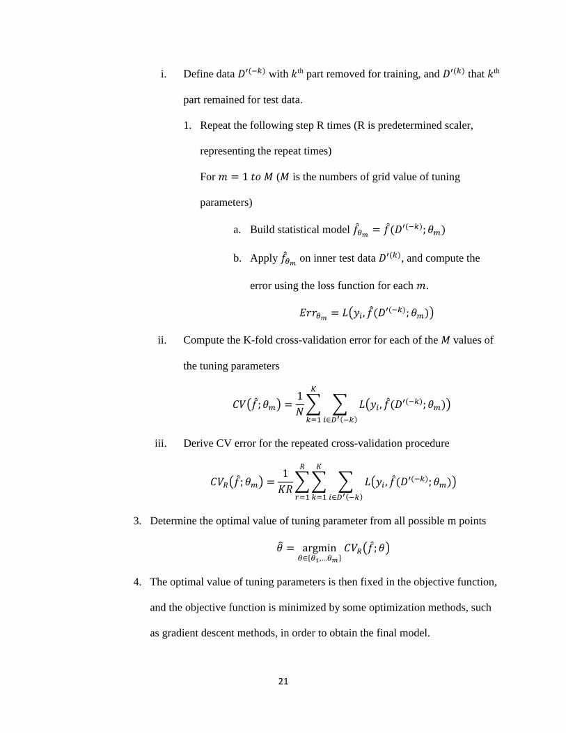
Step 2: classification model building

1. Reduce the training dataset 𝐷 to 𝐷′, where 𝐷′ = (𝐷; 𝑝′). Only the variables

selected in Step 1 are kept in 𝐷′

2. Using same fold that was generated in step 1.


21

i. Define data 𝐷′(−𝑘) with 𝑘th part removed for training, and 𝐷′(𝑘) that 𝑘th

part remained for test data.

1. Repeat the following step R times (R is predetermined scaler,

representing the repeat times)

For 𝑚 = 1 𝑡𝑜 𝑀 (𝑀 is the numbers of grid value of tuning

parameters)

a. Build statistical model 𝑓𝜃𝑚= 𝑓(𝐷′(−𝑘); 𝜃𝑚)

b. Apply 𝑓𝜃𝑚 on inner test data 𝐷′(𝑘), and compute the

error using the loss function for each 𝑚.

𝐸𝑟𝑟𝜃𝑚= 𝐿(𝑦𝑖, 𝑓(𝐷′(−𝑘); 𝜃𝑚))

ii. Compute the K-fold cross-validation error for each of the 𝑀 values of

the tuning parameters


𝑁∑ ∑ 𝐿(𝑦𝑖, 𝑓(𝐷′(−𝑘); 𝜃𝑚))

𝑖∈𝐷′(−𝑘)

𝐾

𝑘=1

iii. Derive CV error for the repeated cross-validation procedure


𝐾𝑅∑ ∑ ∑ 𝐿(𝑦𝑖 , 𝑓(𝐷′(−𝑘); 𝜃𝑚))

𝑖∈𝐷′(−𝑘)

𝐾

𝑘=1

𝑅

𝑟=1

3. Determine the optimal value of tuning parameter from all possible m points

𝜃 = argmin𝜃∈{𝜃1,…𝜃𝑚}

𝐶𝑉𝑅(𝑓; 𝜃)

4. The optimal value of tuning parameters is then fixed in the objective function,

and the objective function is minimized by some optimization methods, such

as gradient descent methods, in order to obtain the final model.

22

To sum up, the method to build and select the predictive model using repeated and nested

cross-validation has more steps than standard single step cross-validation. The complete process

is illustrated in Figure 2.3.2. The inner loop is created to select a candidate subset of features.

While training the model in the inner loop, the V-folds are generated and repeated 𝑅 times to

alleviate the randomness of generation of each fold. This will reduce the variance. The outer loop

will use subset of selected variables to build the final classification model. A simulation study

has been presented evaluating the efficiency and comparing its performance with other standard

methods. Also, the application of this approach has been presented with real dataset.

2.4 Results

2.4.1 Simulation Study

Suppose 𝑌𝑖 is a binary disease outcome, representing the normal cell or cancer cell for

the 𝑖th sample and suppose 𝑿𝒊 is 𝑝-vector that represents the gene expression for the 𝑖th sample.

According to the nature of genetic pathology, there were several characteristics we needed to

consider in our simulation study: (1) some genes are critical to the disease outcome, and those

genes are differentially expressed between cancerous and non-cancerous cells; (2) a few genes

may work as a group to influence the disease outcome and those genes are mutually correlated

[20]. We carry out a cross-sectional simulation study considering the above essential biological

settings. We apply the aforementioned three classification and feature selection methods in the

simulated data to assess the performance of the proposed methods and compare to the standard

cross-validation method.

23

2.4.1.1 Generating the predictors

We simulated our microarray data set with a fixed number of (𝑛 = 100) samples. We

consider a small pool (𝑝 = 1000) and a large pool (𝑝 = 5000) of features. The simulated

design matrix 𝑋 consists of three groups of informative features and remaining are irrelevant

features. The first group is the most important group, which has 1% of all 𝑝 predictors. The

numbers of the features of the three important feature groups are 1%, 2%, and 2% of all

𝑝 predictors, respectively. We use three different strengths of correlations coefficient (𝜌 =

0.3, 0.5, 0.8) for the genes (predictors) within the group but assume that the predictors between

different groups are independent. Thus, we define that 𝑋𝑔, 𝑔 = 1,2,3, indicating the gene

expression for the three groups of important genes. The data is simulated from a multivariate

normal distribution:

𝑋𝑔~𝑀𝑉𝑁(𝝁𝒈, Σ𝑔), 𝑔 = 1, 2, 3. (2.4.1)

where, 𝝁𝒈 = 𝟎, 𝑎𝑛𝑑 Σ𝑔 = 𝑇1

2Γ𝑇1

2, where Γ = [1 ⋯ 𝜌⋮ ⋱ ⋮𝜌 ⋯ 1

], and 𝑇 = [𝜎2 ⋯ 0⋮ ⋱ ⋮0 ⋯ 𝜎2

], 𝜌 is the

pre-determined correlation coefficient. The remaining 95% predictors are simulated from the

standard normal distribution 𝑋𝑖~𝑁(0,1), 𝑖 = (0.05𝑝 + 1), … , 𝑝. Then, we combine the 𝑋𝑔

and 𝑋𝑖 to create our final design matrix 𝑋. In reality, the structure of noise terms could be

very complex. They can be mutually correlated and even correlated with the informative

features. To investigate these complicated scenarios, the more complicated design is

required. We do not address these situations in our simulation study.

24

2.4.1.2 Generating the outcomes

We assume that Y follows a logistic regression with 𝐿𝑜𝑔𝑖𝑡[𝑃(𝑌𝑖 = 1|𝑿𝒊, 𝑿𝒕𝒓𝒖𝒆)] =

𝑿𝒕𝒓𝒖𝒆𝜷𝒕𝒓𝒖𝒆 ,where 𝑿𝒕𝒓𝒖𝒆 indicates a subset vector of “informative” variables of 𝑿𝒊. Therefore,

the outcome 𝑌𝑖 is simulated from a Bernoulli distribution, where 𝑌𝑖~ 𝐵𝑒𝑟𝑛(𝑃𝑖). 𝑃𝑖 is the

Pr (𝑠𝑢𝑏𝑗𝑒𝑐𝑡 𝑖 ℎ𝑎𝑠 𝑑𝑖𝑠𝑒𝑎𝑠𝑒), where 𝑃𝑖 = Pr(𝑌𝑖 = 1|𝑿𝒊) =exp(𝒁𝒊)

1+exp(𝒁𝒊). The model of 𝑍𝑖 = 𝑋𝑖𝛽 is

used to derive the value of 𝑍𝑖. 𝑋𝑖 is the 𝑖th vector of the design matrix as defined in the previous

section, 𝛽 is the vector of coefficients. The value of 𝛽 is set to 5 for important feature group, 3

for secondary feature group, 2 for third feature group, and 0 for all the noise term, denoted as

𝜀𝑖 ~ 𝑁(0,0.01).

In the simulation study, we consider the following six scenarios by considering the

number of pool of variables (small and large), and within-group correlation (low, medium, and

high). The final simulated data is denoted as 𝐷 = {(𝒙𝟏, 𝑦1), (𝒙𝟐, 𝑦2), … , (𝒙𝒏, 𝑦𝑛)}, 𝑖 = 1,2, … , 𝑛.

Each scenario of this simulation is replicated 50 times.

After simulating the data for six cross-sectional scenarios, we apply three different

methods to build the predictive model, including regularization methods with elastic net penalty,

support vector machine, and random forest. The simulation study will investigate the following

questions:

i. Whether applying nested/repeated cross-validation method improves the predictive

performance than applying single cross-validation only.

ii. Comparative study among three different methods to build the predictive model

iii. Comparative study among six different data structures and correlation settings.

25

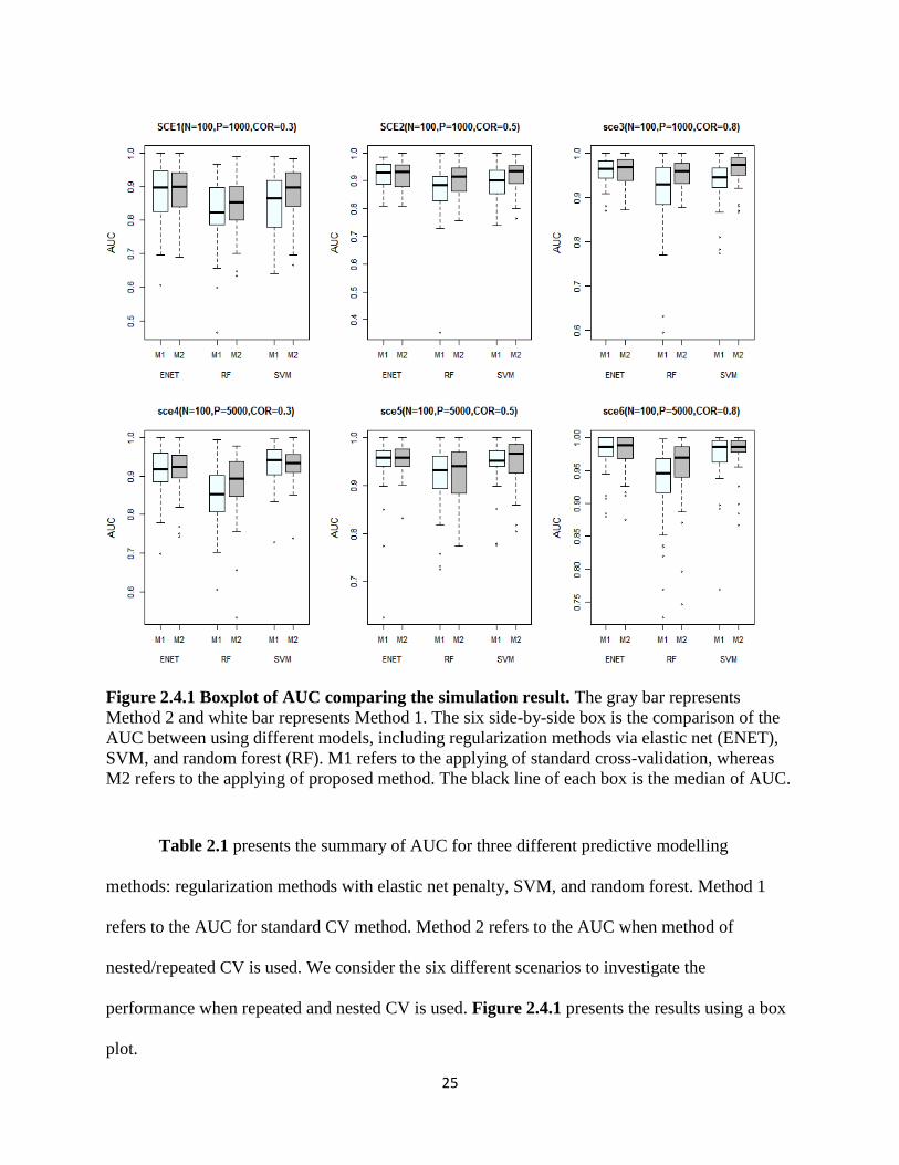
Figure 2.4.1 Boxplot of AUC comparing the simulation result. The gray bar represents

Method 2 and white bar represents Method 1. The six side-by-side box is the comparison of the

AUC between using different models, including regularization methods via elastic net (ENET),

SVM, and random forest (RF). M1 refers to the applying of standard cross-validation, whereas

M2 refers to the applying of proposed method. The black line of each box is the median of AUC.

Table 2.1 presents the summary of AUC for three different predictive modelling

methods: regularization methods with elastic net penalty, SVM, and random forest. Method 1

refers to the AUC for standard CV method. Method 2 refers to the AUC when method of

nested/repeated CV is used. We consider the six different scenarios to investigate the

performance when repeated and nested CV is used. Figure 2.4.1 presents the results using a box

plot.

26

In the simulation study, we investigated the six scenarios to compare the model

performance of building predictive model using standard cross-validation and using

nested/repeated cross-validation. Overall, the prevalence of disease is 0.5. Table 2.1 summarizes

the area under ROC curve (AUC) for the simulation study, the mean and standard deviation of

AUC for 50 replications. We define the building predictive model using standard cross-

validation as Method 1, whereas using repeated and nested cross-validation as Method 2. Table

2.1 shows that the AUC from Method 2 are consistently higher than AUC from Method 1, for

three different statistical learning Methods (regularization Method, SVM, RF). This indicates

that when Method 2 is used, the generalization error (test error) is lower than Method 1.

Therefore, when Method 2 is applied, it provides a better estimated model than Method 1 is used.

In Figure 2.4.1, the gray bar represents the Method 2 and white bar represents the Method 1. The

mean of AUC for Method 2 is consistently higher than AUC for Method 1.

Table 2.1 also enables the comparative study for different statistical modelling strategies

to build the predictive model. The overall AUC is the one of such criteria to compare among

regularization Methods. The simulation study shows the regularization Methods with elastic net

has the best prediction performance than other two modelling strategies. However, since the

model performance is data-driven, the evidence is weak, and it can only justify that

regularization methods with elastic net has better predictive results for this specific simulated

dataset. As well known, the SVM and random forest perform well when data is non-linear, thus,

these two methods can be more appropriate when using in the real data having nonlinear trend.

27

Table 2.1: Summary of area under curve (AUC) (mean and standard deviation) for three feature

selection methods for six different simulation scenarios.

Elastic net Support Vector

Machine Random Forest

Scenario 1, n=100, p=1000, correlation = 0.3, prevalence = 0.513

Method 1 0.8973(0.09) 0.8489(0.08) 0.8271(0.09)

Method 2 0.8997(0.07) 0.8808(0.07) 0.8436(0.07)


Method 1 0.9303(0.05) 0.8943(0.06) 0.8669(0.09)

Method 2 0.9315(0.05) 0.9212(0.05) 0.9028(0.06)


Method 1 0.9604(0.03) 0.9475(0.04) 0.9134(0.08)

Method 2 0.9631(0.02) 0.9497(0.04) 0.9542(0.03)


Method 1 0.9120(0.06) 0.9274(0.05) 0.8503(0.08)

Method 2 0.9154(0.06) 0.9302(0.05) 0.8764(0.08)


Method 1 0.9461(0.06) 0.9475(0.04) 0.9161(0.06)

Method 2 0.9547(0.03) 0.9497(0.04) 0.9268(0.05)


Method 1 0.9780(0.03) 0.9736(0.03) 0.9311(0.06)

Method 2 0.9791(0.02) 0.9793(0.03) 0.9533(0.05

Table 2.2 presents the summary of accuracy for three different predictive modelling

methods: regularization methods with elastic net penalty, SVM, and random forest, the mean and

standard deviation of accuracy for 50 replications. Method 1 refers to the accuracy for standard

CV method. Method 2 refers to the accuracy when method of nested/repeated CV is used.

Figure 2.4.2 presents the results using a box plot.

28

Figure 2.4.2 Boxplot of ACC comparing the simulation result. The gray bar represents Method 2

and white bar represents Method 1. The six side-by-side box is the comparison of the ACC

between using different models, including regularization methods via elastic net (ENET), SVM,

and random forest (RF). M1 refers to standard cross-validation method, whereas M2 refers to the

proposed method. The black line of each box is the median of ACC.

29

Table 2.2: Summary of accuracy (ACC) (mean and standard deviation) for three feature

selection methods for six different simulation scenarios.

Elastic net

Support

Vector

Machine

Random Forest


Method 1 0.7946(0.09) 0.758(0.09) 0.6873(0.10)

Method 2 0.7913(0.08) 0.8833(0.09) 0.7393(0.09)


Method 1 0.810(0.08) 0.778(0.08) 0.7373(0.09)

Method 2 0.809(0.07) 0.8153(0.08) 0.7913(0.09)


Method 1 0.8766(0.06) 0.84(0.08) 0.792(0.10)

Method 2 0.882(0.06) 0.8766(0.07) 0.8606(0.08)


Method 1 0.8033(0.08) 0.76(0.08) 0.686(0.13)

Method 2 0.8186(0.07) 0.84(0.07) 0.7473(0.10)


Method 1 0.8533(0.09) 0.81(0.09) 0.748(0.13)

Method 2 0.8673(0.08) 0.858(0.05) 0.8173(0.09)


Method 1 0.9066(0.06) 0.9(0.07) 0.7953(0.12)

Method 2 0.912(0.06) 0.896(0.07) 0.8667(0.07)

2.4.2 Application to leukemia gene expression data

Two important approaches of data analysis of microarray data includes grouping the

genes to discover broad patterns of biological process, and selecting important genes that are

associated with disease.. We use the leukemia gene expression dataset to investigate the

performance of our proposed method.

The leukemia data, presented in Golub et al. (1999), consists of 47 patients with acute

lymphoblastic leukemia (ALL) and 25 patients with acute myeloid leukemia (AML). Each of the

72 patients had a bone marrow samples obtained at the time of diagnosis. Furthermore, the

30

observations have been assayed with Affymetrix Hgu6800 chips, resulting in 7129 gene

expressions (Affymetrix probes). The Golub data set is possibly the most widely studied and

cited microarray data set [6].In this real data study, we also implement two different methods:

Method 1 and Method 2 as mentioned above The models are trained using training set (38

samples), the AUC and misclassification rate are calculated by using held-out test set (34

samples).

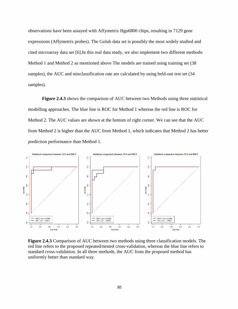
Figure 2.4.3 shows the comparison of AUC between two Methods using three statistical

modelling approaches. The blue line is ROC for Method 1 whereas the red line is ROC for

Method 2. The AUC values are shown at the bottom of right corner. We can see that the AUC

from Method 2 is higher than the AUC from Method 1, which indicates that Method 2 has better

prediction performance than Method 1.

Figure 2.4.3 Comparison of AUC between two methods using three classification models. The

red line refers to the proposed repeated/nested cross-validation, whereas the blue line refers to

standard cross-validation. In all three methods, the AUC from the proposed method has

uniformly better than standard way.

31

Besides looking at ROC and AUC, the misclassification rate is also an important criteria

to assess the model performance. The misclassification rate is computed as: 𝑚𝑖𝑠𝑐𝑙𝑎𝑠𝑠. 𝑟𝑎𝑡𝑒 =

𝐹𝑃+𝐹𝑁

𝑇𝑃+𝑇𝑁+𝐹𝑃+𝐹𝑁. , The terminologies are described in the table below:

Table 2.3 Cross-tabulation of true and predicted classification scenarios

Predicted

Positive Negative

Actual

Positive True Positive (TP) False Negative (FN)

Negative False Positive (FP) True Negative (TN)

A total of 34 bone marrow test samples were used to compute the misclassification rate.

Among the 34 samples, 20 samples are ALL, defined as positive class, and 14 samples are AML,

defined as negative class. The predictive performance measurements can be estimated from

Table 4, for example, the true positive (TP) can be explained as the predictive class is ALL and

actual labelled class is ALL. The misclassification rate then is calculated when the predictive

performance measurements are known.

Table 2.4 Misclassification rate for three different methods

TP FN FP TN Misclassification rate

Enet Method 1 20 8 0 6 23.50%

Method 2 20 5 0 9 14.70%

SVM Method 1 20 4 0 10 11.80%

Method 2 19 1 1 13 5.90%

RF Method 1 20 8 0 6 23.50%

Method 2 20 4 0 10 11.80%

32

Table 2.4 compares AUC result between using single cross-validation (Method 1) in

building the predictive model and using repeated and nested cross-validation (Method 2,

highlighted) in building the predictive model for leukemia cancer gene expression data. For both

methods, three different classifiers are implemented into the framework. For method 1, the

misclassification rates for generalized linear model with elastic net penalty, SVM, and random

forest 23.5%, 11.8%, and 23.5%, respectively. In contrast, for method 2, the misclassification

rates for generalized linear model with elastic net penalty, SVM, and random forest are 14.7%,

5.9%, and 11.8%, respectively. Therefore, to achieve more accurate prediction accuracy when

new data is introduced, the predictive models built using repeated and nested cross-validation

would be better.

2.5 Discussion

In this article, we proposed a more robust cross-validation method for variable selection

and outcome classification. We also demonstrated its application using microarray gene

expression data. However, the method can be applied to any type of high dimensional data where

the concern is to classify the outcomes using a few important variables. The proposed method

applies a nested/repeated cross-validation framework for feature selection and to build the

classification model using selected features. The proposed approach completes the two important

tasks: variable selection and outcome prediction. The outcome of the proposed method can be

utilized further where the research question is concerned about predicting the outcome class

using only a few important biomarkers.

33

Our proposed method uses a combination of repeated and nested cross-validation

technique instead of standard cross-validation method. In our method, double layers of cross-

validation are created. In the inner loop, we perform variable selection and determine the subset

of informative variables, then, the subset of informative variables is used in the outer loop to

estimate the parameters. After the parameters are estimated, the final model is then chosen with

the cross-validation error minimized.

In the simulation study, we present different scenarios under the cross-sectional

biological settings. The simulated dataset is used to build predictive models using three different

statistical methods with two different cross-validation techniques including single cross-

validation and nested/repeated cross-validation. From the results of the simulation study, we

have shown that our proposed method can provide better prediction accuracy in all three

different statistical modeling approaches. Also, the proposed method selects only a few noise

predictors but selects most of true predictors. These results are provided in appendix, Figure a.1

and Figure a.2.

In the application, we used a classical gene expression microarray dataset, the leukemia

dataset from Golub et al. (1999). We used three different statistical modeling approaches

including generalized linear model via elastic net penalty, SVM, and random forest for this

classification task. We found that our proposed method reduces the generalization error

compared to the single cross-validation method.

The proposed method also has some limitations. Rather than using the normal K-fold

cross-validation for model selection, the nested cross-validation requires V folds nested in K

folds, thus, the total 𝐾 × 𝑉 folds are generated for selecting the features and estimating the

tuning parameters. Therefore, the computation time is significantly increased. There is trade-off

34

between the accuracy and computational cost. However, with the development of modern

computing facilities, the computational burden can be minimized using sophisticated

technologies such as the parallel and cloud computing. Table 2.5 shows the comparison of

computational time between two different cross-validation methods. In general, the proposed

method consumes 10 times longer computational time than the standard K-fold cross-validation.

Moreover, the computational time increases when the numbers of candidate features increase.

Also, among three different classification methods, logistic regression via elastic net consumes

the least computational time, whereas the random forest requires the most computational time.

Table 2.5 Computational time for two different methods (in seconds)

Elastic net

Support

Vector

Machine

Random

Forest

Scenario 1, n=100, p=1000, correlation = 0.3

Method 1 2.225 6.299 19.370

Method 2 25.183 82.612 204.812


Method 1 1.718 4.809 16.076

Method 2 19.655 63.661 171.104


Method 1 1.952 5.385 16.733

Method 2 22.744 71.355 177.236


Method 1 3.151 24.001 89.263

Method 2 35.605 327.013 942.643


Method 1 3.555 25.364 91.98

Method 2 35.899 338.954 963.974


Method 1 3.174 23.584 83.389

Method 2 35.236 321.502 908.563

35

Our proposed method can be extended in several ways. (1) the result of feature selection

from the predictive model determines a set of informative genes. When other critical clinical

characteristics are collected, an integrative model can be created by combining the genes and

those clinical covariates. (2) the cross-validation is a commonly used technique for model

selection and model assessment. In our method, we use nested and repeated cross-validation to

select the parameters and to perform model selection. It is also possible to extend the nested

repeated cross-validation in model assessment and to estimate variation of the prediction

accuracy.

In summary, we provide a framework of using nested and repeated cross-validation to

perform feature selection and build a predictive classification model for high dimensional data.

The proposed method is able to provide an improved prediction, and is also able to extract a

subset of informative features from the pool of thousands of features.

36

Chapter 3 Nested cross-validation with ensemble feature selection for

classification model for high-dimensional biological data

Abstract

In recent years, application of feature selection methods in medical and biological

datasets has greatly increased. By using feature selection techniques, subset of relevant

informative features is obtained which gives more interpretable model and improves the model

prediction accuracy. In addition, ensemble learning further provides a more robust model by

combining the results of multiple statistical learning models. In our work, we propose an

algorithm that uses ensemble methods to select the features out of various statistical learning

models to build the classification model with the selected features. Our proposed approach is a

two-step and a two-layer cross-validation method. The first step performs the feature selection in

the inner loop of cross-validation, whereas the second step builds the classification model in the

outer loop of cross-validation. The final classification model, obtained by using the proposed

method, has a higher prediction accuracy than that using the standard cross-validation. The

applications of the proposed method have been presented using both simulated and real dataset.

Keywords: Elastic net, Support Vector Machine, Random Forest, Ensemble Learning, Cross-

Validation, Area Under ROC

37

3.1 Introduction

A typical characteristics of high dimensional data is that the number features measured

on samples are much higher than number of samples. One such example is gene expression data

sets assayed using microarray technology. Selection of the important features to reduce the

dimensionality of the data has always been an important problem in high dimensional data sets.

One important research question in medical application is to build a model that can classify the

subjects into disease subtypes using some selected important features. There are numerous types

of methods available for features selection depending on the purpose of research. As an example,

in microarray gene expression analysis, several gene selection methods based on statistical

analysis and machine learning techniques have been developed to select the informative genes,

including filter methods, wrapper methods, and embedded methods, etc. [19] [36]. In this article

we utilize embedded methods because of the following strengths: (1) embedded methods

consider the correlation among predictor variables, rather than considering the relationship

between outcome and predictors only like filter methods; (2) embedded methods are less

computationally intensive than wrapper methods; (3) embedded methods select features and

build predictive model simultaneously.

In order to build predictive models various techniques are used to select the subset of

features, such as coefficient shrinkage for regularization regression or variable ranking for

random forest. However, different machine learning methods can output different informative

subsets of features, which may lead to differences in prediction accuracy. Ensemble learning is

an effective technique to improve the prediction accuracy and its stability by combining the

output from various methods[37] [38]. Ensemble methods combine multiple learning algorithms

to obtain a predictive performance better than any of the single learning algorithms [39] [40].

38

Ensemble methods have several potential benefits: (1) alleviating the potential of overfitting the

training data [41]; (2) increasing the diversities of machine learning algorithms to obtain a more

aggregated and stable feature subset [42]. Empirically, ensemble learning produces more reliable

results by combining multiple significant diverse models, and seeking the diversities among the

models to improve the prediction accuracy [43].

Ensemble learning has many applications in microarray gene expression studies because

of its unique advantages of dealing with the high-dimensional datasets. Dudoit et al. [44] and

Ben-Dor et al. [45] initially proposed applying bagging and boosting method to classify the

tumor and normal cells in gene expression profiling study. In the last decades, the ensemble

learning has been increasingly developed. For example, Long [46] used several customized

boosting algorithms and Tan and Gilbert [47] proposed ensemble of bagging and boosting

method to obtain a more robust and accurate result in microarray data classification.

In this manuscript, we propose a framework of using nested cross-validation with

ensemble method to construct a model. The training data will be partitioned into two-layers for

cross-validation, feature selection is performed in the inner, whereas classification model is built

in the outer loop. Feature selection is performed using three different embedded learning

methods; regression via elastic net penalty, SVM, and random forest. Then, ensemble method is

used to combine the results out of three different feature selection results. For each classifier

(regression via elastic net penalty, SVM, and random forest), multiple bootstrap datasets are

created for inner layer training data, and corresponding feature subsets are selected. Then, the

feature subsets from all bootstrap datasets are combined using voting strategies, in which the

features that are selected more than 50% times from all bootstrap datasets are then selected as

informative features. After the feature subset is determined in the inner layer, the classification

39

models are built using the selected features in the outer layer. Among all possible classification

models generated in the outer layer, the final model is selected when the cross-validation error is

minimized. To the best of our knowledge, although the idea of using nested cross-validation has

been mentioned elsewhere, no existing literature has proposed or assessed a systematic

framework to utilize nested cross validation with ensemble feature selection at computational

level. Also, no existing literature has utilized this algorithm in microarray gene expression study.

The manuscript is structured as below: Section 2 briefly introduces some statistical

concepts; Section 3 introduces the details of our proposed method; Section 4 provides the

simulation study and results; Section 5 demonstrates the result from several publicly available

microarray datasets; Section 6 discusses the issues of generalizations and limitations.

3.2 Methods

A typical high dimensional dataset can be presented as 𝐷 =

{(𝒙𝟏, 𝑦1), (𝒙𝟐, 𝑦2), … , (𝒙𝒏, 𝑦𝑛)},where 𝑖 = 1,2, 𝑛, indicating 𝑛 subjects or samples; 𝑦𝑖 ∈ {−1,1}

denotes the outcome of 𝑖𝑡ℎ subject; and the p-dimensional vector 𝒙𝒊 defines the observed

variables of subject 𝑖. The dataset is usually high-dimensional with a large number 𝑝 of variables

or features, but a relatively small sample size 𝑛. A statistical model 𝑓 is the estimate of the true

function 𝑓, where 𝑓 is a mapping function:

𝑓: 𝒳 → 𝒴 (3.1)

For the embedded feature selection, the goal is to estimate 𝑓 using the statistical model 𝑓.

When the final 𝑓 is estimated, the subset of features can be simultaneously determined, using

coefficient shrinkage criteria or variable importance ranking criteria. For example, Least absolute

shrinkage and selection operator (Lasso) shrinks the coefficients of some variables to zero, and

40

these variables are removed from the model. Usually, the statistical model 𝑓 is estimated by

optimization of the objective function, which is similar to empirical risk function minimization.

In our work, three different embedded methods are implemented in building the classification

model and feature selection, including regularization regression via elastic net, support vector

machine, and random forest.

3.2.1 Regression via Elastic Net Penalty

The elastic net penalty linearly combines the L-1 norm penalty of Lasso and L-2 norm

penalty of ridge regression [28]. Automatic variable selection by elastic net allows for more than

𝑛 (number of observations) variables to be selected.

L = {[1



𝑇𝜷)] + 𝜆 [(1−𝛼)‖𝛽‖2

2+ 𝛼‖𝛽‖]} (3.2)

The above expression is called objective function, the first component is loss function which

penalizes the misclassification rate, and the second component is the regularization term. Some

of the coefficients are shrunk towards zero, and the corresponding predictors will be removed.

The remaining features are treated as “informative” features. The final model 𝑓 can be used to

predict the future outcome when new data is available.

3.2.2 Support Vector Machine

Support vector machine (SVM) creates a classifier function by constructing hyperplanes

that separate different categories of the training data, and choosing the hyperplane with the

maximal margin between two classes [29]. SVM aims to find the hyperplane with the maximal

margin by solving the following unconstraint optimization problem:

𝐿 = ‖𝑤‖2 + 𝐶 ∑ max (0, 1 − 𝑦𝑖(𝑤𝑇𝜙(𝑥𝑖) + 𝑏)𝑁𝑖=1 (3.3)

41

In expression (3.3), 𝑤 is the weight function that is minimized in order to maximize the

distance 2

‖𝑤‖. 𝐶 is a tuning parameter which is a trade-off between misclassification and size of

margin. Additionally, some Kernel functions are usually utilized, denoted as 𝜙(𝑥𝑖) in (3.3), to

transform the original data from input space to the feature space, which enables linearly

inseparable data in low-dimension to be linearly separable in high-dimension to find the best

hyperplane. One commonly used kernel functions is Gaussian kernel (also called Radial Base

Function), which is given by 𝐾(𝑥, 𝑥′) = 𝜙(𝑥𝑖′)𝜙(𝑥𝑖) = exp (−𝛾 ‖𝑥 − 𝑥′‖

2

). The Gaussian

kernel is used in our work. During the iterative process, variables are ranked according to some

criteria such as area under curve (AUC). The variable importance of each feature can be

explained as the change of AUC when the feature is removed [30]. We determine the importance

of each feature by considering how the performance is influenced without the feature. If

removing a feature worsens the classification performance significantly, the feature is considered

important. The pre-determined numbers of top-ranked features are selected to be the feature

subset.

3.2.3 Random Forest

Random forest for classification is an ensemble method that constructs multiple

bootstrapped decision trees using training samples and combines all the bootstrapped trees to

build the predictive classification model [31]. The detailed steps of random forest can be

described as follows (1) bootstrap samples of size 𝑛 are drawn from data 𝐷, denoted as 𝐷𝑏 =

{(𝑥1𝑏 , 𝑦1𝑏), … (𝑥𝑛𝑏 , 𝑦𝑛𝑏)}, to create a decision tree; (2) train the decision tree 𝑓𝑏 based on the

bootstrap samples 𝐷𝑏 to get 𝑓𝑏. In growing the single decision tree, m variables are randomly

selected at each node of the tree. The m selected variables split the tree to achieve the minimum

42

error; (3) grow the tree to largest extent possible (no pruning tree); (4) repeat the previous three

steps to build B bootstrapped decision trees. Then, the final random forest model is obtained by

combining the different decision trees using majority vote, denoted as 𝑓 = 𝑚𝑜𝑑𝑒(𝑓1, … , 𝑓𝐵).

Variable importance (also known as predictor ranking) is a critical measurement for both

decision trees and random forests which depends on the contribution to the tree by each

predictor. Random forest utilizes variable importance to rank the variables. Permutation

techniques can be used with random forests to measure the variable importance, the details of

computing the variable importance for each variable can be found elsewhere [32].

Features that produce large values for this score are ranked as more important than

features with small values. The important variables are then selected by the ranked variable

importance.

3.2.4 Ensemble methods

Ensemble methods combine results from various different classifiers to achieve more

accurate classification results on the training set as well as accurate prediction performance on

the test set [38]. There are many ensemble methods used in high-dimensional biological data

analysis [48, 49]. To achieve a better generalization performance on the test set, ensemble

methods usually utilize bias-variance trade-off. For example, bootstrap aggregating (bagging)

achieves a better generalization performance by decreasing the variance [50]; whereas boosting

achieves this by decreasing bias [51]. Ensemble method can also be viewed as several types:

ensemble by single classifier with multiple inputs; ensemble by multiple classifiers with one

input; ensemble by multiple classifiers with multiple inputs. It is also important to indicate that

the performance of final ensemble model relies on the diversities of classifiers and training

43

datasets, in other words, the final ensemble model can capture varieties of different classifiers or

data to achieve a more stable and robust final ensemble model. For example, suppose we want to

ensemble 25 base models, and each model has error rate of 0.35. If the models are independent

and uncorrelated, the error rate of ensemble model (more than 50% models are wrong) is

∑ (25𝑖

) 𝜖𝑖(1 − 𝜖)25−𝑖 = 0.0625𝑖=13 . This error rate is lower than any of individual based model.

Also, to illustrate the process of ensemble method, we can generate multiple new training

datasets with some variants of original training data (i.e. generating the bootstrap resample

dataset from original training dataset), and, each newly generated training data is used to build

several individual models. Then the individual models are aggregated to approximate the “best”

classification model by some voting strategies.

There are three the most popular ensemble approaches: bootstrap aggregating (bagging),

boosting, and stacked generalization. Bootstrap aggregating (bagging) combines the

classification results of the given classifiers from multiple bootstrapped datasets. With bagging,

the original training dataset is used to resample multiple bootstrapped datasets. The given

classifier (i.e. logistic regression) is used to train the multiple bootstrapped datasets and the

results of all bootstrapped datasets are then combined to build the final bagging model. Bagging

reduces variance and seeks to avoid overfitting. Boosting is another ensemble approach. The

central idea of boosting and its variant algorithms is to create a strong statistical model using a

set of weak classification models (also called weak learners), the weak learner is defined as any

classification model which is better than random guess. Most boosting algorithms iteratively

combine weak learners to find a final strong learner. Stacked generalization (stacking) introduces

a two-level approach to find the final model. The first level is to create the model using multiple

models/approaches. The second level is to estimate the input together with outputs of each model

44

to estimate the weights and to determine which models perform well given these input data.

Then, stacking combines those models with their weights.

There are two steps of our proposed method: (1) feature selection in inner layer and (2)

classification model building in outer layer. In the manuscript, we primarily utilize the ensemble

method by multiple classifiers (logistic regression, SVM, random forest) with multiple inputs

(bootstrapped inner training dataset) for ensemble feature selection. To carry out the ensemble

feature selection, the multiple bootstrapped inner training datasets are generated, then, different

classifiers are implemented for these inner training datasets. With each inner training dataset and

each classifier, a feature subset is built, and the final feature subset is determined by using

majority of voting of all the feature subsets. The details of our proposed method is given in next

section.

3.2.5 Nested cross-validation with ensemble feature selection and classification models

Our proposed method has two goals. The first goal is to select the subset of features and

the second goal is to find the optimal value of tuning parameters for classification model and to

choose the best model. The proposed method has two layers of cross-validation: inner layer and

outer layer. In the inner layer, the target is feature selection using ensemble method, whereas in

the outer layer, the target is build the final classification model using selected features from inner

layer. Once the model is built the prediction accuracy is also estimated. The optimal feature

subset increases the prediction accuracy and decreases the computational cost and also makes the

final classification model more interpretable. Figure 3.2.1 illustrates the complete process of the

proposed method.

45

Figure 3.2.1. Flow chart of feature selection with ensemble method, and building classification

model using the selected features. In model selection part, we create a two-layer cross-validation

to train the data and to choose the final model. In inner loop of cross-validation, for each inner

train dataset, we create 𝐵 bootstrapped datasets, three different classifiers, SVM, random forest,

and logistic regression via elastic net are used to train the bootstrapped datasets for each inner

training dataset to obtain the feature subsets. The best candidate feature subset is then determined

by combining all the feature subsets from inner loops using majority vote. When the feature

subset is chosen, it is used in outer loop to select the tuning parameters and build the

classification model. The final model is evaluated by external test data.

The main framework of the proposed method can be summarized as follows. To

illustrate the complete process of proposed method, we divide the method into two steps. The

first step is ensemble feature selection in the inner loop and the second step is classification

model selection in the outer loop. In the proposed method, there are two layers of cross-

validation, the training data is partitioned into K folds of roughly equal size; this layer is called

outer loop of cross-validation, and each dataset with Kth part removed is called inner training

46

dataset, so that there are K different inner training dataset. Then, each inner training dataset is

partitioned into V folds; this is called inner loop of cross-validation. In this way there are V sub-

folds nested within each of the K folds. The multiple classifiers with multiple inputs ensemble

method is then used for ensemble feature selection. To achieve the ensemble feature selection,

bootstrap resampling technique is used for all K inner training datasets to create B (B is the

predetermined numbers of size of bootstrap samples) bootstrapped inner training datasets. Next,

three different classifiers (logistic regression via elastic net, SVM, and random forest) are used to

train B bootstrapped inner training datasets to select feature subsets using various criteria

(coefficient shrinkage method for logistic regression and, variable ranking for SVM and random

forest). In total, each classifier creates B different feature subsets. The final feature subset is

determined using voting strategy, where any feature is selected more than 50% times (>3×𝐵

2) is

selected as the informative feature. After the feature subset is determined, the irrelevant features

are removed and only the selected features are used in the next step. The step 2 is to build the

final classification model in the outer loop. The simplified training data is used in this step, in

which the irrelevant features are removed, and only the selected features from step 1 are retained.

In this way, the final classification model is built using three different classification methods

(logistic regression via elastic net, SVM, and random forest) individually. The final classification

model can predict the future outcome when new data is introduced, as well as evaluates the

performance of selected feature subset. The detail of the algorithm is given as follow:

Step 1: variable selection using ensemble method

1. Divide the training dataset 𝐷 into 𝐾 folds of roughly equal size


47

i. Define data 𝐷−𝑘 with 𝑘th part removed as the outer training data, and 𝐷𝑘 with

only 𝑘th part remained as the outer test data.

a. Draw a bootstrap sample from 𝐷−𝑘, denoted as 𝐷𝑏−𝑘. Randomly divide

dataset 𝐷𝑏−𝑘 into 𝑉 folds of roughly equal size. Let 𝑏 = 1, … , 𝐵 is the

numbers of bootstrap dataset. Note that, the numbers of bootstrap dataset

𝐵 can be viewed as tuning parameter, which is determined by cross-

validation to optimize the model performance, but at here, to save the

computational time, we fix the value of 𝐵.

a) Define data (𝐷𝑏−𝑘)

−𝑣with 𝑣th part of 𝐷𝑏

−𝑘 removed as the inner training

data, and 𝐷𝑏𝑘𝑣 with only the 𝑣th part remained for inner test data.

For 𝑣 = 1 𝑡𝑜 𝑉

For 𝑚 = 1 𝑡𝑜 𝑀 (𝑀 is the number of grid value of the tuning

parameters)

1) Build statistical model 𝑓𝜃𝑚= 𝑓((𝐷𝑏

−𝑘)−𝑣

; 𝜃𝑚) using

logistic regression via elastic net penalty.

2) Apply 𝑓𝜃𝑚 on inner test data (𝐷𝑏

−𝑘)𝑣, and compute the error

using the loss function in inner test set.

𝐸𝑟𝑟𝜃𝑚= ∑ 𝐿 (𝑦𝑖, 𝑓𝑏((𝐷𝑏

−𝑘)𝑣

; 𝜃𝑚))


b) Compute the V-fold cross-validation error for each 𝑚, therefore, there

are 𝑚 different CV errors. 𝑁𝑣 is the number of observations in inner

loop for 𝑘th part.

48

𝐶𝑉(𝑓𝑏; 𝜃𝑚) =1

𝑁𝑣∑ ∑ 𝐿 (𝑦𝑖, 𝑓𝑏((𝐷𝑏

−𝑘)𝑣

; 𝜃𝑚))


𝑉

𝑣=1

b. Determine the optimal value of tuning parameter 𝜃𝑚 from all possible m

points

𝜃𝑚 = argmin𝜃∈{𝜃1,…𝜃𝑚}

𝐶𝑉(𝑓𝑏; 𝜃𝑚)

c. The optimal values of tuning parameters are then fixed in the objective

function, and the objective function is minimized using numerical

optimization techniques, such as gradient descent. [34] [35]. When the

final model is chosen, and feature subset is determined by variable ranking

method or coefficient shrinkage methods. Let 𝑠𝑏(. ) be an indicator

function, represented by:

𝑠𝑏(𝑥) = {1 𝑖𝑓 𝑥 𝑖𝑠 𝑠𝑒𝑙𝑒𝑐𝑡𝑒𝑑 𝑏𝑦 𝑡ℎ𝑒 𝑓𝑖𝑛𝑎𝑙 𝑚𝑜𝑑𝑒𝑙 0 𝑖𝑓 𝑥 𝑖𝑠 𝑛𝑜𝑡 𝑠𝑒𝑙𝑒𝑐𝑡𝑒𝑑 𝑏𝑦 𝑡ℎ𝑒 𝑓𝑖𝑛𝑎𝑙 𝑚𝑜𝑑𝑒𝑙

The feature subset can be denoted as:

𝐹𝑆𝑏𝐸𝑁= {𝑠𝑏(𝑝1), 𝑠𝑏(𝑝2), … , 𝑠𝑏(𝑝𝑝)}

d. Repeat the above process (a-c) for 𝐵 times, thus, we draw 𝐵 different

bootstrap datasets, and obtain 𝐵 different feature subsets, 𝐹𝑆𝑏𝐸𝑁=

{𝑠𝑏(𝑝1), 𝑠𝑏(𝑝2), … , 𝑠𝑏(𝑝𝑝)}.

e. Repeat the above process (a-d), implement another two classifiers, support

vector machine and random forest for the same bootstrap inner. As a

result, we can obtain 𝐵 different feature subsets, 𝐹𝑆𝑏𝑆𝑉𝑀=

{𝑠𝑏(𝑝1), 𝑠𝑏(𝑝2), … , 𝑠𝑏(𝑝𝑝)}, 𝑏 = 1,2, … , 𝐵 when SVM is implemented,

49

and 𝐵 different feature subsets, 𝐹𝑆𝑏𝑅𝐹= {𝑠𝑏(𝑝1), 𝑠𝑏(𝑝2), … , 𝑠𝑏(𝑝𝑝)}, 𝑏 =

1,2, … , 𝐵 when random forest is implemented.

f. Since we have three different classifiers, and each classifier can create 𝐵

different feature subsets, then the “winner” feature subset is defined as:

𝐹𝑆𝑘 = {𝑓𝑠(𝑝1), 𝑓𝑠(𝑝2), … , 𝑓𝑠(𝑝𝑝)}

where 𝑓𝑠𝑘(. ) is an indicator function, indicating whether the 𝑎 feature is

selected more than 50% across the three classifiers with B bootstrap

samples, and represented by

𝑓𝑠𝑘(𝑥) = {1 𝑖𝑓 𝑥 𝑖𝑠 𝑠𝑒𝑙𝑒𝑐𝑡𝑒𝑑 𝑔𝑟𝑒𝑎𝑡𝑒𝑟 𝑜𝑟 𝑒𝑢𝑞𝑎𝑙 𝑡𝑜

3𝐵

2 𝑡𝑖𝑚𝑒𝑠

0 𝑖𝑓 𝑥 𝑖𝑠 𝑠𝑒𝑙𝑒𝑐𝑡𝑒𝑑 𝑙𝑒𝑠𝑠 𝑡ℎ𝑎𝑛 3𝐵


2. Since we have 𝐾 folds, we have 𝐾 different “winner” feature subsets; we

compute the number of times that each feature is selected. Then, the final

feature subset is defined as:

𝐹𝑆𝑓𝑖𝑛𝑎𝑙 = {𝑓𝑠(𝑝1), 𝑓𝑠(𝑝2), … , 𝑓𝑠(𝑝𝑝)}, where 𝑓𝑠(. ) is an indicator function,

indicating whether a feature 𝑥 is selected, and represented by

𝑓𝑠(𝑥) = {1 𝑖𝑓 𝑥 𝑖𝑠 𝑠𝑒𝑙𝑒𝑐𝑡𝑒𝑑 𝑔𝑟𝑒𝑎𝑡𝑒𝑟 𝑜𝑟 𝑒𝑢𝑞𝑎𝑙 𝑡𝑜

𝐾


0 𝑖𝑓 𝑥 𝑖𝑠 𝑠𝑒𝑙𝑒𝑐𝑡𝑒𝑑 𝑙𝑒𝑠𝑠 𝑡ℎ𝑎𝑛 𝐾


3. This step creates a subset of 𝑝′ selected variables, where 𝑝′ is the number of

selected variables. Then, we move to step 2.

Step 2: classification model building

1. Reduce the training dataset 𝐷 to 𝐷′, where 𝐷′ = (𝐷; 𝑝′). Only the variables

selected in Step 1 are kept in 𝐷′

50

2. Using the same folds that were generated in step 1.


i. Define data 𝐷′(−𝑘) with 𝑘th part removed as the training dataset, and

𝐷′(𝑘) with 𝑘th part remained as the test data.

1. Repeat the following steps R times (R is a predetermined scaler,

representing the repeating times)

For 𝑚 = 1 𝑡𝑜 𝑀 (𝑀 is the numbers of grid value of tuning

parameters)

a. Build statistical model 𝑓𝜃𝑚= 𝑓(𝐷′(−𝑘); 𝜃𝑚)

b. Apply 𝑓𝜃𝑚 on the inner test data 𝐷′(𝑘), and compute the

error using the loss function for each 𝑚.

𝐸𝑟𝑟𝜃𝑚= 𝐿 (𝑦𝑖, 𝑓 (𝐷′(−𝑘)

; 𝜃𝑚))

c. Compute the K-fold cross-validation error for each of

the 𝑀 values of the tuning parameters, 𝑁 is the number

of observations in out loop for 𝑘th part.


𝑁∑ ∑ 𝐿(𝑦𝑖, 𝑓(𝐷′(−𝑘); 𝜃𝑚))

𝑖∈𝐷′(−𝑘)

𝐾

𝑘=1

ii. Derive CV error for the repeated cross-validation procedure


𝐾𝑅∑ ∑ ∑ 𝐿(𝑦𝑖 , 𝑓(𝐷′(−𝑘); 𝜃𝑚))

𝑖∈𝐷′(−𝑘)

𝐾

𝑘=1

𝑅

𝑟=1

3. Determine the optimal value of tuning parameter from all possible m points

𝜃 = argmin𝜃∈{𝜃1,…𝜃𝑀}

𝐶𝑉𝑅(𝑓; 𝜃)

51

4. The optimal value of tuning parameters is then fixed in the objective function,

and the objective function is minimized by some optimization methods, such

as gradient descent methods, in order to obtain the final model.

3. 3 Results

3.3.1 Simulation Study

Suppose 𝑌𝑖 is a binary disease outcome, indicating whether the cell is normal or

cancerous for the 𝑖th sample and suppose 𝑿𝒊 is a 𝑝-dimensional vector that represents the gene

expression for the 𝑖th sample. According to the nature of genetic pathology, there were several

characteristics we needed to consider in our simulation study: (1) some genes are critical to the

disease outcome, and those genes are differentially expressed between cancerous and non-

cancerous cells; (2) a few genes may work as a group to influence the disease outcome and those

genes are mutually correlated [20]. We carry out a cross-sectional simulation study considering

the above two scenarios. We apply the aforementioned three classification and feature selection

methods in the simulated data to assess the performances of the proposed methods with

comparison to the standard cross-validation method.

3.3.1.1 Generating the predictors

We simulated our microarray data set with a fixed number of (𝑛 = 100) samples. We

consider a small pool (𝑝 = 2000) and a large pool (𝑝 = 5000) of features. The simulated

design matrix 𝑋 consists of three groups of informative features and remaining are irrelevant

features. The first group is the most important group, which has 1% of all 𝑝 predictors. The

numbers of the features of the three important feature groups are 1%, 2%, and 2% of all

𝑝 predictors, respectively. We use three different strengths of correlations coefficient (𝜌 =

52

0.3, 0.5 𝑎𝑛𝑑 0.8) for the genes (predictors) within the group but assume that the predictors

between different groups are independent. Thus, we define that 𝑋𝑔, 𝑔 = 1,2,3, indicating the

gene expression for the three groups of important genes. The data is simulated from a

multivariate normal distribution:

𝑋𝑔~𝑀𝑉𝑁(𝝁𝒈, Σ𝑔), 𝑔 = 1, 2, 3. (3.3.1)

where, 𝝁𝒈 = 𝟎, 𝑎𝑛𝑑 Σ𝑔 = 𝑇1

2Γ𝑇1

2, where Γ = [1 ⋯ 𝜌⋮ ⋱ ⋮𝜌 ⋯ 1

], and 𝑇 = [𝜎2 ⋯ 0⋮ ⋱ ⋮0 ⋯ 𝜎2

], 𝜌 is the

pre-determined correlation coefficient. The remaining 95% predictors are simulated from the

standard normal distribution 𝑋𝑖~𝑁(0,1), 𝑖 = (0.05𝑝 + 1), … , 𝑝. Then, we combine the 𝑋𝑔

and 𝑋𝑖 to create our final design matrix 𝑋. In reality, the structure of noise terms could be

very complex. They can be mutually correlated and even correlated with the informative

features. To investigate these complicated scenarios, the more complicated design is

required. We do not address these situations in our simulation study.

3.3.1.2 Generating the outcomes

We assume that Y follows a logistic regression with 𝐿𝑜𝑔𝑖𝑡[𝑃(𝑌𝑖 = 1|𝑿𝒊, 𝑿𝒕𝒓𝒖𝒆)] =

𝑿𝒕𝒓𝒖𝒆𝜷𝒕𝒓𝒖𝒆 ,where 𝑿𝒕𝒓𝒖𝒆 indicates a subset vector of “informative” variables of 𝑿𝒊. Therefore,

the outcome 𝑌𝑖 is simulated from a Bernoulli distribution, where 𝑌𝑖~ 𝐵𝑒𝑟𝑛(𝑃𝑖). 𝑃𝑖 is the

Pr (𝑠𝑢𝑏𝑗𝑒𝑐𝑡 𝑖 ℎ𝑎𝑠 𝑑𝑖𝑠𝑒𝑎𝑠𝑒), where 𝑃𝑖 = Pr(𝑌𝑖 = 1|𝑿𝒊) =exp(𝒁𝒊)

1+exp(𝒁𝒊). The model of 𝑍𝑖 = 𝑋𝑖𝛽 is

used to derive the value of 𝑍𝑖. 𝑋𝑖 is the 𝑖th vector of the design matrix as defined in the previous

section, 𝛽 is the vector of coefficients. The value of 𝛽 is set to 5 for important feature group, 3

for secondary feature group, 2 for third feature group, and 0 for all the noise term, denoted as

𝜀𝑖 ~ 𝑁(0,0.01).

53

In the simulation study, we consider the following six scenarios by considering the

number of pool of variables (small and large), and within-group correlation (low, medium, and

high). The final simulated data denoted as 𝐷 = {(𝒙𝟏, 𝑦1), (𝒙𝟐, 𝑦2), … , (𝒙𝒏, 𝑦𝑛)}, 𝑖 = 1,2, … , 𝑛.

The simulation for each scenario is replicated 50 times.

The simulated dataset of above six cross-sectional scenarios are used to build the

classification models and compare the prediction performance among classification models using

standard cross-validation and those using our proposed method. In addition, the simulated dataset

is partitioned into training and test datasets, the training data is used to select the feature subsets

and then to build the classification model; whereas the test data is used to evaluate the model

performance. For our proposed method, we carry out the nested cross-validation with ensemble

method for feature selection. Two layer of cross-validation is constructed to build the final

classification model, where ensemble feature selection is performed in the inner layer to find the

informative feature subsets, and three different classifiers are used to build the final classification

model in outer layer, including regularization methods with elastic net penalty, support vector

machine, and random forest. The simulation study will investigate the following questions:

i. Whether applying nested cross-validation method with ensemble feature selection

improves the predictive performance than applying single cross-validation only.

ii. Comparative study among three different classification methods to build the

predictive model when feature subset is selected by ensemble method.

iii. Comparative study among six different data structures and correlation settings.

Table 3.1 presents the summary of AUC of classification model for three different

classifiers: regularization methods with elastic net penalty, SVM, and random forest, the mean

and standard deviation of AUC for 50 replications. Method 1 refers to standard CV method.

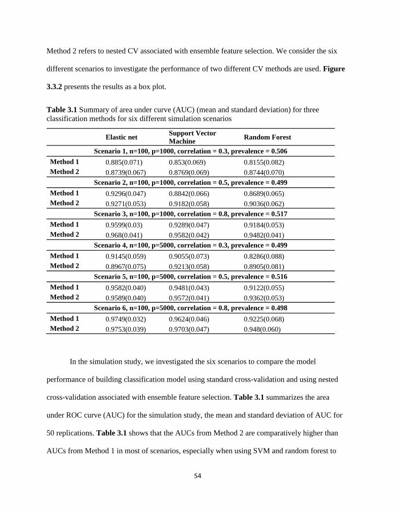
54

Method 2 refers to nested CV associated with ensemble feature selection. We consider the six

different scenarios to investigate the performance of two different CV methods are used. Figure

3.3.2 presents the results as a box plot.

Table 3.1 Summary of area under curve (AUC) (mean and standard deviation) for three

classification methods for six different simulation scenarios




Method 1 0.885(0.071) 0.853(0.069) 0.8155(0.082)

Method 2 0.8739(0.067) 0.8769(0.069) 0.8744(0.070)


Method 1 0.9296(0.047) 0.8842(0.066) 0.8689(0.065)

Method 2 0.9271(0.053) 0.9182(0.058) 0.9036(0.062)


Method 1 0.9599(0.03) 0.9289(0.047) 0.9184(0.053)

Method 2 0.968(0.041) 0.9582(0.042) 0.9482(0.041)


Method 1 0.9145(0.059) 0.9055(0.073) 0.8286(0.088)

Method 2 0.8967(0.075) 0.9213(0.058) 0.8905(0.081)


Method 1 0.9582(0.040) 0.9481(0.043) 0.9122(0.055)

Method 2 0.9589(0.040) 0.9572(0.041) 0.9362(0.053)


Method 1 0.9749(0.032) 0.9624(0.046) 0.9225(0.068)

Method 2 0.9753(0.039) 0.9703(0.047) 0.948(0.060)

In the simulation study, we investigated the six scenarios to compare the model

performance of building classification model using standard cross-validation and using nested

cross-validation associated with ensemble feature selection. Table 3.1 summarizes the area

under ROC curve (AUC) for the simulation study, the mean and standard deviation of AUC for

50 replications. Table 3.1 shows that the AUCs from Method 2 are comparatively higher than

AUCs from Method 1 in most of scenarios, especially when using SVM and random forest to

55

build the classification model. This indicates that when Method 2 is used, the generalization error

(test error) is lower than that from Method 1. Therefore, when Method 2 is applied, it tends to

provide a better estimated model than and a better prediction accuracy, in most cases.

Specifically, the AUCs are not very different when using logistic regression via elastic net to

build to classification model, which means the prediction performances are equally reliable. On

the contrary, when using the SVM or random forest to build the classification, the AUCs from

Method 2 are higher than AUCs from Method 1, which indicates the ensemble feature selection

can provide more robust feature subset, and prediction of classification model is more accurate.

Table 3.2 Summary of accuracy (ACC) for three classification methods for six different

simulation scenarios with ensemble feature selection results.




Method 1 0.7998(0.084) 0.7366(0.099) 0.7118(0.084)

Method 2 0.7882(0.077) 0.7621(0.092) 0.7836(0.082)


Method 1 0.8377(0.072) 0.7656(0.089) 0.7532(0.080)

Method 2 0.8433(0.067) 0.8123(0.085) 0.8232(0.080)


Method 1 0.8863(0.064) 0.8238(0.084) 0.8177(0.082)

Method 2 0.8864(0.066) 0.8808(0.063) 0.8637(0.065)


Method 1 0.814(0.062) 0.7857(0.0957) 0.701(0.082)

Method 2 0.7969(0.091) 0.825(0.07842) 0.785(0.073)


Method 1 0.8786(0.065) 0.8338(0.11) 0.7986(0.071)

Method 2 0.8813(0.068) 0.8723(0.069) 0.8628(0.070)


Method 1 0.897(0.062) 0.8647(0.087) 0.8028(0.089)

Method 2 0.9046(0.066) 0.9032(0.067) 0.8654(0.074)

56

Table 3.2 presents the summary of accuracy of classification model for three different

classification methods, the mean and standard deviation of accuracy for 50 replications. Method

1 refers to standard CV method. Method 2 refers to nested CV associated with ensemble feature

selection. We consider the six different scenarios to investigate the performance of two different

CV methods are used. Figure 3.3.3 presents the results as a box plot. The results of accuracy of

classification model shows the same conclusion as AUC.

Table 3.1 and Table 3.2 also present the comparison among different statistical

modelling strategies to build the classification model. The overall AUC is one of such criteria to

compare among regularization methods. The simulation study showed the regularization

methods with elastic net had the best prediction performance among three modelling strategies.

The main reason could be that the data is simulated from multivariate normal distributions.

However, since the model performance is data-driven, the evidence is weak, and it can only

justify that regularization methods with elastic net has better predictive results for this specific

simulated dataset. As known, SVM and random forest perform well when model is non-linear,

thus, these two methods may be more appropriate when the real data has nonlinear trend.

57

Figure 3.3.2 Boxplot of AUC comparing the simulation results. The gray box represents Method

2 and the white box represents Method 1. M1 refers to standard cross-validation, whereas M2

refers to the proposed method. The six side-by-side boxes represent the comparison of the AUCs

across different models, including regularization methods via elastic net (ENET), SVM, and

random forest (RF).

58

Figure 3.3.3 Boxplot of Accuracy comparing the simulation results. The gray box represents

Method 2 and the white box represents Method 1. M1 refers to standard cross-validation,

whereas M2 refers to the proposed method. The six side-by-side boxes represent the comparison

of the AUCs across different models, including regularization methods via elastic net (ENET),

SVM, and random forest (RF).

59

3.3.2 Application to leukemia and prostate gene expression data

We now implement our proposed method in several publicly available microarray gene

expression datasets to investigate the feature selection result and classification performance. The

first microarray gene expression data that we used consists of 47 patients with acute

lymphoblastic leukemia (ALL) and 25 patients with acute myeloid leukemia (AML). Each of the

72 patients had bone marrow samples obtained at the time of diagnosis. The specimens were

assayed with Affymetrix Hgu6800 chips, resulting in 7129 gene expressions (Affymetrix probes)

[8]. The second microarray gene expression data was derived from 52 prostate tumors and 50

non-tumor prostate samples from patients undergoing surgery. After prepressing, 6033 genes

were remained [52] for the study.

In the real case study, we used ensemble learning with nested cross-validation to generate

the informative feature subset. Then, three different classifiers, regularization regression via

elastic net, SVM, and random forest, were used to predict the class label of the test data. Then,

two criteria including AUC and misclassification rate (1 − 𝑝𝑟𝑒𝑐𝑖𝑠𝑖𝑜𝑛) were used to evaluate the

performance of classification with given feature subsets. The misclassification rate was

computed as: 𝑚𝑖𝑠𝑐𝑙𝑎𝑠𝑠. 𝑟𝑎𝑡𝑒 =𝐹𝑃+𝐹𝑁

𝑇𝑃+𝑇𝑁+𝐹𝑃+𝐹𝑁. The terminologies used are described in Table

3.4.

Table 3.4 Cross-tabulation of true and predicted classification scenarios

Predicted

Positive Negative

Actual

Positive True Positive (TP) False Negative (FN)

Negative False Positive (FP) True Negative (TN)

60

Table 3.4 shows the result of evaluation of prediction performance of two gene

expression datasets. For the Leukemia study by Gloub et.al, the AUCs for all methods were

greater than 0.95 when three different classifiers were used to predict the class label of the test

data, which means predicting future outcome using the selected feature subset can result in a

good precision. Also, the misclassification rates were 21%, 6%, and 12% for regularization

regression via elastic net, SVM, and random forest, respectively. Here, regularization regression

seems more likely to misclassify the class label of the test data. On the contrary, SVM provides a

reliable result with only two samples misclassified. For the Prostate study by D.Singh et.al, the

AUCs of all three methods were close to one, and misclassification rates were lower than 10%.

As a result, the selected feature subset leads to an accurate prediction.

Table 3.5 Misclassification rate for three different classification methods using ensemble

feature selection

Cancer Method AUC TP FP FN TN Misclassification

rate

Prostate

ENET 0.9822 15 0 2 13 0.07

SVM 0.9734 12 3 0 15 0.1

RF 0.9954 15 0 1 14 0.03

Leukemia

ENET 0.9692 20 0 7 7 0.21

SVM 0.9714 19 1 1 13 0.06

RF 0.9767 20 0 4 10 0.12

3.4 Discussion

In this manuscript, we proposed an ensemble feature selection method for feature

selection and classification for high dimensional data. In our proposed method, we used nested

cross-validation technique to perform the feature selection in the inner cross-validation loop and

61

to build final classification model in the outer loop CV. When performing feature selection in the

inner loop CV, we generated an ensemble feature subset by combining the feature selection

results of several classifiers. We showed that ensemble method can improve the stability of

selected features, and also improve the prediction accuracy when the new data is introduced.

The proposed method can select the subset of informative features and provide a reliable

prediction using the selected features. Our simulation study investigated feature selection

efficiency and prediction accuracy of the proposed method under a few different scenarios. The

simulation settings consider different correlation levels among features and different sizes of

datasets. From the result of the simulation study, we confirm that the proposed method is able to

select a subset of most informative features. Also, the prediction performances are justifiable

when different classifiers are implemented to predict the class label of the test data using the

selected feature subset. Then, we applied the proposed method to some public gene expression

data. When the proposed method was used, the informative genes were selected. With different

classifiers used to predict the outcome of the test data based on feature subset of our proposed

method, the AUC and precision both were high. The results indicate that the proposed ensemble

method can more correctly classify the samples based on the features. Both the simulation study

and application demonstrated that the proposed method works better than single layer cross-

validation. Moreover, the proposed method selects only a few noise predictors but selects more

of true predictors than standard k-fold cross-validation. These results are provided in appendix,

Figure a.3 and Figure a.4.

Our proposed method can be extended in multiple ways. First, in our proposed method,

we only combined three different classifiers, the regularization regression via elastic net, SVM,

and random forest. All of these three classifiers are called embedded methods. An extension of

62

the proposed method would be an ensemble of other methods beyond embedded methods such as

filter methods, in fact, many filter methods are commonly used in microarray gene expression

data. Second, we fit the classification model using the selected molecular features only. In fact,

other clinical characteristics are critical to the clinical outcomes. When we have the feature

subsets of informative genes, it is possible to add the clinical covariates into the data to build the

classification and predictive model. Third, nested cross-validation is applicable for both model

selection and model assessment. For our proposed method, nested CV is used for model selection

only. We determined the hyper-parameters in the inner CV, and the tuning parameters in the

outer CV. The prediction performance was evaluated based on the test data. We can also use

nested CV in another way; tuning the parameters in the inner loop, and evaluating the prediction

performance in the outer loop so that we can obtain the variation of the prediction accuracy.

The limitation of our proposed method is also obvious with respect to computational cost.

When using the nested cross-validation with ensemble feature selection, the computational

burden significantly increased; especially when many methods that are being combined. It

requires much more computational time than using standard cross-validation or not using

ensemble methods. Table 3.5 shows the comparison of computational time between two

different cross-validation methods. In general, the proposed method consumes approximate 200

times longer computational time than the standard K-fold cross-validation. Moreover, the

computational time increases when the numbers of candidate features increase. Also, among

three different classification methods, logistic regression via elastic net consumes the least

computational time, whereas the random forest requires the most computational time.

63

Table 3.5 Computational time for two different methods (in seconds)




Method 1 3.641 7.416 20.429

Method 2 640.076 640.076 640.076


Method 1 3.126 6.449 19.492

Method 2 589.436 589.436 589.436


Method 1 3.183 6.672 19.400

Method 2 593.736 593.736 593.736


Method 1 10.666 34.296 108.678

Method 2 2868.639 2868.639 2868.639


Method 1 9.187 30.417 105.711

Method 2 2779.062 2779.062 2779.062


Method 1 8.558 28.163 93.976

Method 2 2619.424 2619.424 2619.424

However, it is reasonable to sacrifice some computation time to improve the prediction

performance, as well as to generate a more stable feature subset. Additionally, parallel

computing or cloud computing can be used to alleviate the computational burden.

To sum up, we provided a framework to extract the most informative features from high

dimensional data using a nested cross-validation with ensemble feature selection method, and

then to build the classification model using the selected informative features.

64

Chapter 4 Application of nested cross-validation with ensemble feature

selection in cervical cancer research using microarray gene expression data.

Abstract

Cervical cancer remains one of the most common types of cancer for women, and major

causes of cancer-related death worldwide. Several studies have attempted to identify the genes

that are associated with cervical cancer. In our work, we used two publicly available cervical

cancer microarray gene expression datasets to achieve the following goals: (1) find the

informative genes which are associated with cervical cancer; (2) find the informative genes

which are associated with different subtypes of cervical cancer. We used the statistical learning

methods with nested cross-validation with ensemble feature selection to achieve the above goals.

Using GSE data on cervical cancer, a total of 96 selected genes were found to be differentially

expressed between normal samples and cervical cancer samples; among these 96 genes, 33 genes

were biologically validated or known genes for cervical cancer in the literature, and 13 genes

were found to play important roles in a top-scored gene pathway for cervical cancer. Using

TCGA data, we also found 19 differentially expressed gene between two subtypes of cervical

cancer, squamous cell carcinoma and adenocarcinoma. Further functional analysis is needed with

these genes in order to understand the etiology of cervical cancer.

Keywords: Cervical Cancer, Classification, Ensemble Learning, Cross-Validation, Gene

selection, Pathway Analysis

65

4.1 Introduction

Cervical cancer is a type of cancer that occurs in the cervix cells, at the lower end of the

uterus that connects the upper vagina [53]. Every year around 528,000 new cases are diagnosed

worldwide, leading to 266,000 deaths [54]. Cervical cancer is the second most common cancer

and the major cause of death, compared to any other gynecological cancers [55].

The major risk factor to cause cervical cancer is persistent infections with carcinogenic

Human papillomavirus infection (HPV), a sexually transmitted infection [56]. Other risk factors

include smoking, weak immune system, and inappropriate sexual behaviors, but these are less

important than HPV infections [53]. According the world cancer report, 90% of cervical cancer

cases are squamous cell carcinoma (SCC), whereas 10% are adenocarcinoma, and a small

number are other sub type of cervical cancer [54].

Although cervical cancer can be treated with radiation or surgery in early stages, it is

difficult to detect cervical cancer at early stage [57, 58]. Cervical cancer is incurable if it is

metastasized [57]. Therefore, it is important to undertake studies to understand association

between molecular process and clinical consequence. Various researches have been conducted to

investigate the cervical cancer and its carcinogenesis. There are two major types of studies, the

first is to find the differentially expressed genes between normal cells and cancerous cells, and

the second is to further investigate the informative genes for only cancerous cells. For example,

Wong et.al utilized analysis of gene expression profiles to find the most aberrantly expressed

genes for cervical cancer in Hong Kong females [59]. Martin CM et.al identified some

differentially expressed genes for disease diagnosis and therapy using gene expression profiling

in cervical cancer between healthy and cancer cells [60]. On the other hand, a few recent works

have utilized only the cancer tumors in order to identify cancer subtypes using several types of

66

molecular data including gene expression data In the integrated genomic and molecular

characterization of cervical cancer project conducted by the Cancer Genome Atlas (TCGA),

research revealed notable APOBEC mutagenesis patterns, and identified several novel

significantly mutated genes for cervical cancer [61]. The integrative clustering also identified

three subtypes, two subtypes within squamous cell carcinoma (SCC): keratin-low and keratin-

high squamous and the third adenocarcinoma rich subtype.

Microarray technology is a popular biological technique to measure the gene expression

levels of thousands of genes in a single experiment. Microarray technique is widely used in

cancer classification [62]. The primary goals of cancer classification are (1) to distinguish the

differentially expressed genes which may regulate the different biological consequences, i.e., the

normal cells or cancerous cells; and (2) to predict outcome when new patients’ gene expression

data are available. The microarray gene expression data are usually high-dimensional, having a

relatively small number of samples compared to the huge numbers of genes [63, 64]. Therefore,

feature selection method that selects the important genes out of thousands of genes is critical.

Feature selection is very important because it can determine a subset of genes that are associated

with the disease which can be studied further for practical therapeutic attempts. Furthermore, it

can help building the prediction models with important gene attributes which will consume less

computational resources, avoid the overfitting issues, and improve the prediction accuracy [64].

Various statistical learning methods have been used in feature selection. The statistical

learning methods can build the classification models to predict the future outcomes. The

classification models utilize several criteria, such as variable ranking, to select informative

features [19] [36] [65]. On the other hand, ensemble learning is also an effective technique to

improve feature selection stability and prediction accuracy [37] [38]. The ensemble model is

67

built by combining different individual statistical learning models which results in a better

predictive performance than any of the individual models [39] [40]. Ensemble method can

achieve several potential benefits: (1) alleviating the potential of overfitting the training data

[41]; (2) increasing the diversities of statistical learning algorithms to obtain a more aggregated

and stable feature subset [42]. Empirically, ensemble learning provides more reliable results

when combining significant diversity among the models, and seeks to promote diversity among

the models to improve the prediction accuracy [43] [46] [47].

Usually, there are two types of parameters that are estimated in statistical learning

models: weight coefficients and tuning parameters. Weight coefficients are estimated using

gradient descent methods and the tuning parameters are estimated using cross validation methods

by minimizing the objective functions in both cases. Gradient descent method is a standard

method in fitting the statistical learning models and is available with many software packages.

Cross-validation generates different folds of training data, and selects the optimal value of tuning

parameters when cross-validation error is minimized. Standard cross validation method is also

available with many software packages, such as caret.

In this manuscript, we utilize a novel ensample method in the cervical cancer disease

classification. We utilize statistical learning methods on microarray gene expression data,

emphasizing on finding differentially expressed genes and predicting the future outcomes based

on the selected genes. Specifically, we apply the framework of nested cross-validation with

ensemble feature selection and then construct classification models, using two publicly available

cervical cancer gene expression datasets. To achieve this goal, we build a two-step model: the

first step is to perform feature selection and the second is to use the selected features to build the

final classification model. The manuscript is designed as: section 2 briefly describes the data and

68

introduces the methods; section 3 provides results and our findings; section 4 discusses the issues

of generalizations and limitations.

4.2 Methods and Materials

4.2.1 Data description

There are two publicly available cervical cancer related gene expression datasets that are

used in our study. The first dataset is devoted to find the differentially expressed genes between

normal cells and cancer cells. The second dataset is to further investigate the gene expression of

the cancer cells to study the cancer sub-types.

The publicly available gene expression dataset was downloaded from Gene Expression

Omnibus (GEO), a public functional genomics data repository [66, 67]. The GEO Series number

is GSE9750 (https://www.ncbi.nlm.nih.gov/geo/query/acc.cgi?acc=GSE9750). The original

study that utilized this dataset investigated the cervical cancer tumorigenesis [68]. This dataset

contains a total 66 samples, with 42 tumor samples and 24 normal samples. There are total

22,283 microarray chip probes.

The second data was downloaded from The Cancer Genome Atlas (TCGA) website

(https://tcga-data.nci.nih.gov/docs/publications/cesc_2017/). The dataset has been used to

investigate important differentially expressed genes between two histologic subtypes of cervical

cancer: SCC and adenocarcinoma, using statistical learning methods [61].The dataset consists of

20,533 genes assayed on 178 samples, including 144 SCC samples, 31 adenocarcinoma samples,

and 3 adenosquamous samples.

https://www.ncbi.nlm.nih.gov/geo/query/acc.cgi?acc=GSE9750

https://tcga-data.nci.nih.gov/docs/publications/cesc_2017/

69

4.2.2 Statistical background

A typical high-dimensional dataset can be presented as:

𝐷 = {(𝒙𝟏, 𝑦1), (𝒙𝟐, 𝑦2), … , (𝒙𝒏, 𝑦𝑛)}, 𝑤ℎ𝑒𝑟𝑒 𝑖 = 1,2, , … 𝑛.

indicating 𝑛 subjects or samples. Here, 𝑦𝑖 ∈ {−1,1}, denotes the outcome of 𝑖𝑡ℎ subject, and the

p-dimensional vector 𝒙𝒊 defines the observed features of subject 𝑖. The dataset is usually high-

dimensional with a large number of variables or features 𝑝, but a small sample size of 𝑛. In high-

dimensional gene expression data analysis, a statistical model 𝑓 is built to estimate the true

function 𝑓, where 𝑓 is a mapping function:

𝑓: 𝒳 → 𝒴 (4.1)

When 𝑓 is estimated, the final model 𝑓 can simultaneously determine the subset of

important features, using coefficient shrinkage criteria or variable importance ranking criteria.

Usually, the statistical model 𝑓 is estimated by optimization of the objective function. In our

work, three different classification methods are implemented in building the classification model

and feature selection, including regularization regression via elastic net, support vector machine,

and random forest.

Logistic Regression via Elastic Net Penalty

The elastic net penalty combines the L-1 norm penalty of least absolute shrinkage and

selection operator (lasso) and L-2 norm penalty of ridge regression [28]. Logistic regression via

elastic net penalty can complete an automatic variable selection and allow for more than

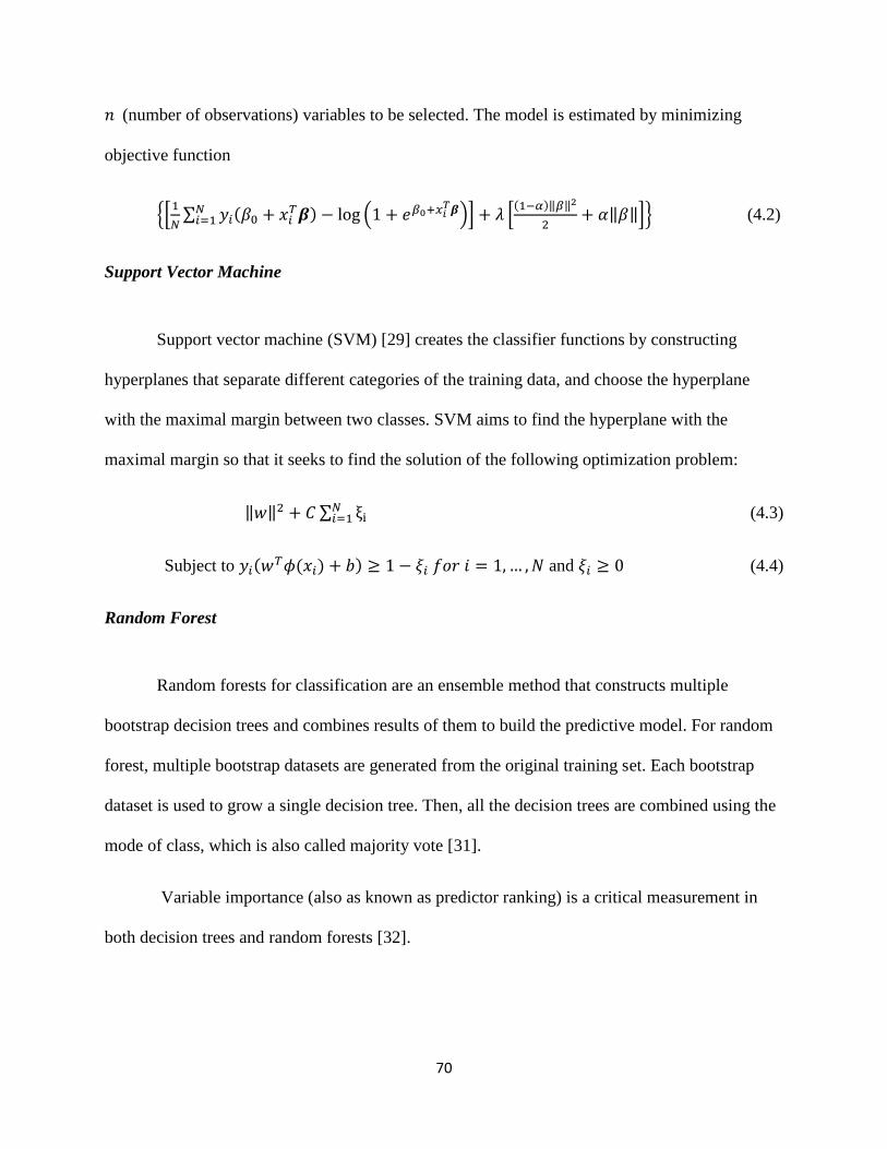
70

𝑛 (number of observations) variables to be selected. The model is estimated by minimizing

objective function

{[1



𝑇𝜷)] + 𝜆 [(1−𝛼)‖𝛽‖2

2+ 𝛼‖𝛽‖]} (4.2)

Support Vector Machine

Support vector machine (SVM) [29] creates the classifier functions by constructing

hyperplanes that separate different categories of the training data, and choose the hyperplane

with the maximal margin between two classes. SVM aims to find the hyperplane with the

maximal margin so that it seeks to find the solution of the following optimization problem:

‖𝑤‖2 + 𝐶 ∑ ξi𝑁𝑖=1 (4.3)

Subject to 𝑦𝑖(𝑤𝑇𝜙(𝑥𝑖) + 𝑏) ≥ 1 − 𝜉𝑖 𝑓𝑜𝑟 𝑖 = 1, … , 𝑁 and 𝜉𝑖 ≥ 0 (4.4)

Random Forest

Random forests for classification are an ensemble method that constructs multiple

bootstrap decision trees and combines results of them to build the predictive model. For random

forest, multiple bootstrap datasets are generated from the original training set. Each bootstrap

dataset is used to grow a single decision tree. Then, all the decision trees are combined using the

mode of class, which is also called majority vote [31].

Variable importance (also as known as predictor ranking) is a critical measurement in

both decision trees and random forests [32].

71

4.2.3 Framework of feature selection and classification model construction

The statistical learning models are used in high-dimensional biological data for several

applications including disease classification and differential expression analysis of genes.

Ensemble learning methods are used to combine the classification models to construct a more

robust model and to additionally improve the model performance. In our work, we implement a

framework of using statistical learning and ensemble learning methods to select features and

build classification models.

Nested cross-validation with ensemble feature selection

We now introduce the nested cross-validation with ensemble feature selection method.

To apply nested cross-validation, we first prepare our training data into outer and inner training

datasets: (1) the original training data is partitioned into 𝐾 folds of roughly equal size, for outer

loop of cross-validation (Figure 4.2.1). There are the 𝐾 different folds in this layer, and each

(𝐾−1)

𝐾× 100% data are called outer training data, and (

1

𝐾) × 100% data are called outer test data.

The first step is feature selection. In the inner loop, for each of 𝐾 outer training datasets,

bootstrap technique is used to generate 𝐵 multiple training datasets to create inner training

datasets, thus there are 𝐾 × 𝐵 inner training datasets. Then ensemble feature selection can be

applied as follows: (1) within each 𝐾 × 𝐵 inner training datasets, create the grid of possible

values of tuning parameters; (2) implement one of abovementioned classifiers (logistic

regression via elastic net, SVM, and random forest) associated with V fold cross-validation on

the bootstrap dataset to train the model and compute the cross-validation error for each potential

value of tuning parameters; then, determine the optimal model for the bootstrap re-sample data,

and select a subset of informative features; (3) repeat (2) for all 𝐵 bootstrap samples, with which

72

we select 𝐵 subsets of informative features; (4) repeat (2) and (3) for the two other classifiers;

here, we select other 𝐵 subsets of features for each of classifiers, leading to a total of 3 × 𝐵

feature subsets; (5) repeat (1) – (4) for all 𝐾 folds, then, leading to a total of 3 × 𝐾 × 𝐵 feature

subsets; (6) the final feature subset is determined as the set including: any feature is selected

more than 3×𝐾×𝐵

2 times, and all features in the set are considered as informative features.

Figure 4.2.1. Flow chart of feature selection with ensemble method, and building classification

model using the selected features. In model selection part, a two-layer cross-validation is used to

train the data and to choose the final model. In inner loop of cross-validation, 𝐵 bootstrap

datasets are created from outer training data; then, three different classifiers, SVM, random

forest, and logistic regression via elastic net are used to train the bootstrap datasets to obtain the

feature subsets. The final feature subset is then determined by combining all the feature subsets

from the inner loops using majority vote. The final feature subset is used in the outer loop to

select the tuning parameters and build the classification model. The final model is evaluated by

external test data.

The second step is model construction. Only informative features selected from the first

step are kept and all other features are removed. The selected features are used in the outer loop

of training data, then classification models are built using repeated K fold cross-validation

73

techniques, and the final model is chosen when the average CV error is minimal. The final

classification model can be used to predict the future outcomes. The mathematical details of this

framework are presented in the Supplementary file II.

4.3 Results

4.3.1 Result using GSE9750 data

The gene expression microarray dataset GSE9750 contains 66 samples, associated with

22,283 probes. In our study, we used only the probes that had gene annotation which brings the

number of genes down to 12,502 genes. There are 42 cervical cancer samples, as well as 24

normal cells. We used 80% of samples (54 samples) as training data to perform the feature

selection, and classification model construction. The remaining 20% (12 samples) was used as

external test data, to assess the prediction accuracy of the classification model built on the

training data.

Figure 4.3.1 Flow chart for GSE9750 gene expression data-preprocessing

74

A major task in gene expression analysis was to find a subset of differentially expressed

genes between normal and cancerous cells. We applied the previously introduced framework,

nested cross-validation with feature selection ensemble for classification. In this framework, the

cross-validation (CV) method was nested/repeated, the evaluation criteria was area under receiving

operating curve (AUC) and the classification methods were logistic regression via elastic net

penalty, SVM, and random forest.

Table 4.1 Summary of AUC and accuracy of classifying normal and cancerous cells

Classifier methods

Enet SVM Random forest

AUC Accuracy AUC Accuracy AUC Accuracy

CV method Method 1 1 1 1 1 0.96

Method: Nested/repeated cross-validation with ensemble feature selection

Table 4.1 presents the results of AUC and accuracy of classifying normal and cancer

cells for the GSE9750 microarray gene expression dataset. The CV method applied nested cross-

validation with feature selection ensemble for feature selection step. When the 96 differentially

expressed genes were selected, three different classification method were applied to build the

final classification model. The final classification models from three classifiers could achieve

remarkably high the AUCs and accuracies. It acquired 100% prediction accuracy and AUC

achieved to 1, which meant our classification models based on ensemble feature selection

method were able to construct an accurate statistical model in predicting the unseen data.

Additionally, a total of 96 genes were selected from nested cross-validation with feature

75

selection technique and we determined the top-selected 30 genes to report. The complete list of

selected genes are presented in the appendix as Table a.1 and Table a.2.

Table 4.2 References of frequently selected genes from CCDB

Frequently selected genes and references

Gene Name #Reference Reference Details

CDKN2A 26 [59, 70-72]

Cyclin Dependent

Kinase Inhibitor 2A

CRNN 1 [59] Cornulin

MAL 3 [59, 75, 76]

Mal, T-Cell

Differentiation Protein

MCM2 3 [59, 77, 78]

Minichromosome

Maintenance Complex

Component 2

TPX2 1 [68]

TPX2, Microtubule

Nucleation Factor

CDK2 1 [79]

Cyclin Dependent

Kinase 2

EDN3 2 [59, 80] Endothelin 3

KRT13 3 [73, 74] Keratin 13

Then, we further investigated the selected 96 differentially expressed genes. In fact, it was

possible that features (genes) were statistically significant for certain dataset but biologically

irrelevant to cervical cancer. Therefore, additional investigation based on the histological or

pathological study was required. We first compared differentially expressed genes that were

selected from our proposed method to the biologically validated or known cervical carcinogenesis.

Cervical cancer database (CCDB, http://crdd.osdd.net/raghava/ccdb) [69] is a manually curated

database that record experimentally validated genes that are thought, or are known to be involved

in cervical carcinogenesis. There are a total 537 validated genes in CCDB that are linked with

cervical cancer processes [69]. 33 genes that were selected from our methods were also present in

http://crdd.osdd.net/raghava/ccdb

76

CCDB. Table 4.2 lists some highly selected genes from our methods, and some references of these

genes from other cervical cancer related papers.

Table 4.3 Top-ranked diseases built from selected differentially expressed genes

Categories Diseases or Functions

Annotation

Molecules

Cell Cycle Mitosis of cervical cancer

cell lines

AURKA,KPNB1,NDC80,NEK2,SPAG5,ST

IL

Cell Morphology,

Cellular

Compromise

Multinucleation of

cervical cancer cell lines

AURKA,KIF14,NEK2

Cell Cycle Mitotic exit of cervical

cancer cell lines

KPNB1,NEK2

Cell Morphology,

Cellular Function

and Maintenance

Autophagy of cervical

cancer cell lines

CDKN2A,CRYAB

Cell Cycle M phase of cervical

cancer cell lines

AURKA,KIF14,NDC80

Cellular

Movement

Migration of cervical

cancer cell lines

CA9,ESR1,KANK1

Cell Death and

Survival

Apoptosis of cervical

cancer cell lines

CDKN2A,ESR1,KIF14,NASP,NDC80,SPA

G5

Cell Death and

Survival

Cell death of cervical

cancer cell lines

CDKN2A,ESR1,KIF14,KPNB1,NASP,NDC

80,SPAG5

Cell Death and

Survival

Cell viability of cervical

cancer cell lines

AURKA,CDK2,CDKN2A,NUP210

Cell Cycle,

Cellular

Movement

Cytokinesis of cervical

cancer cell lines

AURKA,KIF14

Another biologically knowledge-based analysis for the selected genes is pathway

analysis. Pathway analysis helps to understand the roles of genes on knowledge-based pathways.

It also helps to understand distinct cell process with differentially expressed genes. Ingenuity

Pathway Analysis (IPA) contains large numbers of literatures related to genetic research, and

helps to further exploring and illustrating the information depending on the biological

knowledge-based libraries [81]. We used IPA software in order to complete the biological-based

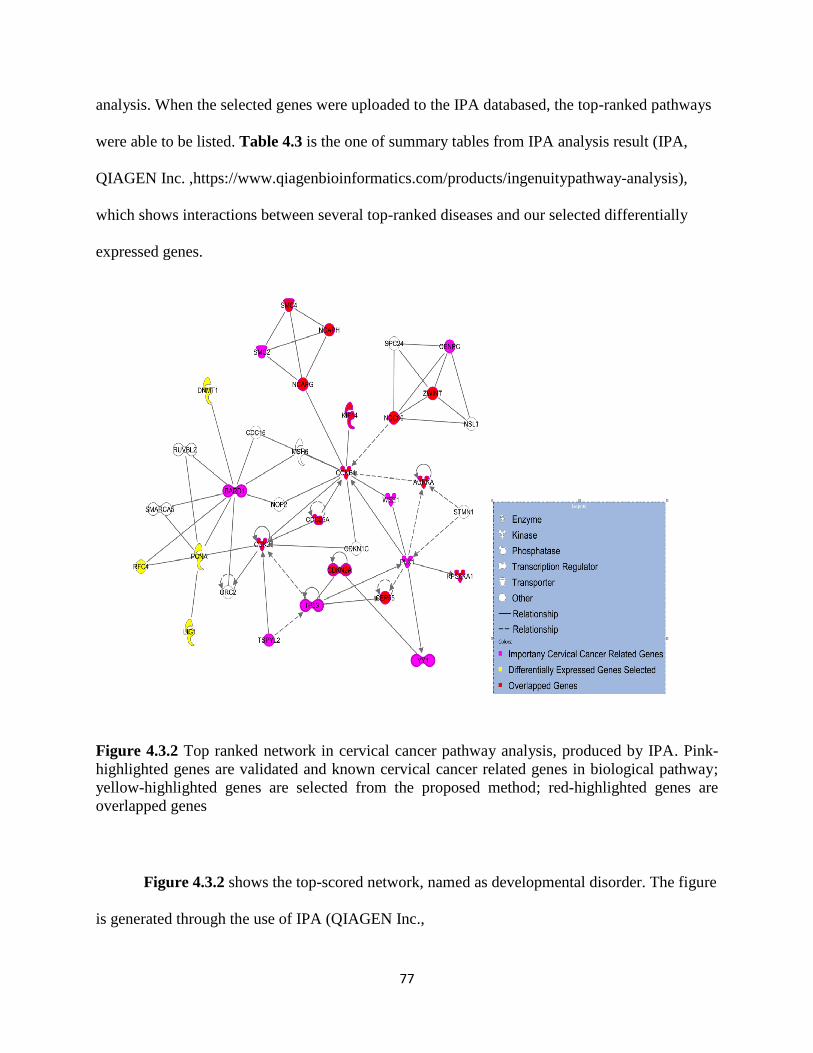
77

analysis. When the selected genes were uploaded to the IPA databased, the top-ranked pathways

were able to be listed. Table 4.3 is the one of summary tables from IPA analysis result (IPA,

QIAGEN Inc. ,https://www.qiagenbioinformatics.com/products/ingenuitypathway-analysis),

which shows interactions between several top-ranked diseases and our selected differentially

expressed genes.

Figure 4.3.2 Top ranked network in cervical cancer pathway analysis, produced by IPA. Pink-

highlighted genes are validated and known cervical cancer related genes in biological pathway;

yellow-highlighted genes are selected from the proposed method; red-highlighted genes are

overlapped genes

Figure 4.3.2 shows the top-scored network, named as developmental disorder. The figure

is generated through the use of IPA (QIAGEN Inc.,

78

https://www.qiagenbioinformatics.com/products/ingenuity-pathway-analysis). In this network,

pink-highlighted genes were validated and known cervical cancer related genes in biological

pathway, for example, CDNK2A, CCNB1, and KIF14 were related to the pathway of apoptosis

of cervical cancer cell lines; yellow-highlighted genes were selected from our method; and, red-

highlighted genes were overlapped between experimentally known cervical cancer related genes

and our selected differentially expressed genes. Figure 4.3.2 presents that 13 out of 21

biologically validated cervical cancer related genes overlapped with our selected differentially

expressed genes. Except these 13 genes shown in abovementioned network, other genes also

played the important role in other biologically cervical cancer related networks.

To sum up, the statistical learning methods selected a subset of differentially expressed

genes based on the training data, and had a high prediction accuracy for the test data. Also, about

1/3 (33 genes) of the selected genes were validated or known to be cervical cancer related genes,

and 13 of them were found to have important roles in a top-scored cervical cancer pathway.

4.3.2 Result from TCGA data

The integrative TCGA cervical cancer project contains several datasets, and we used only

microarray gene expression data in our work. There are 178 samples with a total of 20,533 genes

assayed on them. The major goal was to classify two cervical cancer types: squamous and

adenocarcinoma. Figure 4.3.3 illustrates the flow chart for data preparation. Among 175 valid

samples with 19,038 genes, we chose 80% of samples (141 samples) as training data, whereas

79

the remaining 34 samples as test data, utilized to assess the model.

Figure 4.3.3. Flow chart for TCGA gene expression data-preprocessing

The primary goal of our work was to find a subset of informative genes which were

differentially expressed between two types of cervical cancer. We applied the previously

introduced framework, nested cross-validation with ensemble feature selection and classification.

In this frameworks, the CV method we used was nested/repeated, and the classification methods

were logistic regression via elastic net penalty, SVM, and random forest.

Table 4.4 Summary of AUC and accuracy of classifying two types of cervical cancer

Classifier method

Enet SVM Random forest

AUC Accuracy AUC Accuracy AUC Accuracy

CV method Method 0.9762 94.11% 0.9405 88.23% 0.9821 94.11

Method: Nested/repeated cross-validation with ensemble feature selection

80

Table 4.4 presents the results that AUC and accuracy of classifying two types of cervical

cancer: squamous and adenocarcinoma. The CV method applied nested/repeated cross-validation

with ensemble feature selection. After the differentially expressed genes were selected, three

different classification methods were implemented to build the final classification model for

further prediction. A total of19 genes were selected as differentially expressed genes. The

complete list of selected genes are presented in the appendix as Table a.3.

Figure 4.3.4 Heat map for 19 selected genes and all 175 cervical cancer samples

81

Figure 4.3.4 presents the heat map of the samples and the selected genes. The heat map

shows almost all genes selected from the proposed method were upregulated in first cluster

(adenocarcinoma), and downregulated in second cluster (squamous). The heatmap shows that the

expression level of samples are different between two cancer subtypes.

Moreover, in the ensemble feature selection step, the selection criterion was set to 0.5,

which means that the gene is considered as differentially expressed if it is selected more than

50% times of all iteration. However, in some cases, this criterion can be lowered for exploring

more biologically meaningful genes. For example, if selection criterion had been changed to be

0.4, a total 56 differentially expressed genes would have been selected. Figure 4.3.5 shows the

two third of the selected genes were up-regulated in adenocarcinoma and the remaining one third

selected genes were down-regulated in adenocarcinoma. The choice of selection criterion is

somewhat subjective, and is guided by research interests. If the research is designed to build a

parsimonious model, then higher selection threshold should be used, whereas id the research is

designed to explore more potential genes to classify the subtypes of cervical cancer, then a

relatively lower threshold can be used.

82

Figure 4.3.5. Heat map for 56 selected genes and all 175 cervical cancer samples

4.4 Discussion

In this manuscript, we applied a statistical learning method on microarray gene

expression analysis, for cervical cancer research. There were two major goals in this research, (1)

to classify normal cells and cancerous cells; (2) to classify two sub-types of cervical cancer cells,

squamous and adenocarcinoma. Two publicly available cervical cancer microarray databases

were used, one from GEO public database, and another from the TCGA cervical cancer

83

integrative molecular characterization project. We used cross-validation and statistical learning

models to select the associated genes and to predict the outcomes of new data based on the

classification models built.

The data was analyzed by statistical learning methods. We utilized three different

classifiers: logistic regression via elastic net, support vector machine, and random forest. For

each classifier, we used nested cross-validation, rather than a standard K-fold cross-validation.

The benefits were more biology oriented, (1) first we selected the informative genes from inner

loop and built a more genetically interpretable classification model which using selected genes

only; (2) the primary goal in microarray gene expression studies was selecting important genes,

rather than only emphasizing on prediction as other statistical learning problems. We also

applied the ensemble learning methods to aggregate the feature selection results from multiple

classification models and to construct a more robust feature subset.

Our proposed classification model with nested cross-validation could detect the

informative differentially expressed gene subsets for major goals. From the statistical

perspective, our proposed method could select a set of differentially expressed genes. Also, the

prediction accuracy was remarkably high to predict the class for test data. From the biological

perspective, the selected genes were also meaningful. Several selected genes play important roles

in the known biological pathways or diseases. Moreover, some of them acted as critical parts in

cell progression network. Furthermore, additional exploratory studies might reveal whether other

selected features have potential association with cervical cancer. Our work might provide a more

clinically accurate therapeutic targets for cervical cancer, since we have shown that the genes we

selected were differentially expressed in two different subtypes of cervical cancer. Our work can

be extended by including important clinical covariates in building the classification models.

84

Our work also has limitations. We utilized the nested cross-validation rather than the

standard K fold cross-validation. This increases the computational burden. Our proposed method

might take much more computational time on training the models and summarizing the results.

However, the development of faster computational abilities can alleviate this problem.

In summary, we have successfully implemented a nested cross-validation and ensemble

feature selection method on microarray gene expression datasets for cervical cancer research.

Our method has detected a pool of disease associated genes. Some of these genes have also been

shown to play roles in a biological pathway of cervical cancer. Further investigation is needed to

explore the significance of other genes in other identified pathway in the etiology of cervical

cancer.

85

Chapter 5 Summary and future directions

In this dissertation work, we primarily used the statistical learning methods for feature

selection and building the classification model based on high-dimensional biological dataset. The

most important part of this study is to apply statistical learning methods to build a parsimonious

model with informative predictors with high prediction accuracy.

For high-dimensional data analysis, the numbers of predictors are usually larger

compared to the numbers of observations. Therefore, selecting a subset of predictors which

contain most information is very important. Also, prediction is another critical task for high-

dimensional data analysis. Various statistical learning methods are designed to achieve this goal.

Two types of parameters need to be determined for these methods: weight coefficients and

tuning parameters. Weight coefficients are usually estimated by gradient descent, rather than

ordinary least square. Tuning parameters are usually determined by cross-validation. When the

optimal tuning parameters are chosen, the objective function is optimized and the final model

can be built. The final model can be used for predicting the outcomes for new data, as well as

selecting the most important features using various criteria.

In this dissertation, we designed the framework of nested-cross-validation for feature

selection and classification model construction, which selects the informative features in the

inner layer of cross-validation and builds the final classification model in the outer loop. When

the framework is fully explained, different statistical learning methods can be implemented, such

as logistic regression via elastic net penalty. We then expanded the previous work by using

ensemble methods to combine the feature selection results from different classification method,

to obtain a more robust feature subset. At last, we used the nest cross-validation with feature

86

selection ensemble on the realistic microarray gene expression data to find the informative genes

associated with cervical cancer. The analyses were completed using R software. The R codes and

summary will be available upon request.

To sum up, our proposed method performed well on both simulated datasets and real

datasets, resulting in parsimonious models with high prediction accuracy on testing data. Also,

our method selected a set of differentially expressed genes, some of which have been validated

as cervical cancer related genes as compared to other published works and others might need to

be explored further. One of the drawbacks of the proposed methods is the computational time,

the computational time is much longer than using the traditional k-folds cross-validation

techniques. However, by scarifying the computational time, our proposed method outperform

traditional k-folds cross-validation in stability and robustness of feature, by excluding most of

noise features. This can be beneficial when further investigation of selected associated features.

Also, our proposed method can slightly improve the classification accuracy than the k-fold cross-

validation techniques.

Other limitations of the dissertation included lack of enough replications in simulation

studies, and balanced samples between disease and healthy samples. The number of replicates

for each simulation scenario was set to be 50, due to the lengthy computation time. With 50

replicates for each scenario, the simulation was able to show the improvement of mean of AUC

when the proposed methods were used, but the small number of replicates may not be enough to

show whether the improvement in AUC was statistically significant . To detect the statistical

significance, more replicates are needed. However, due to the heavy computational burden,

generating more replicates would significantly increase the computational time. Furthermore, the

prevalence of cases for simulation was set to 0.5 only. In reality, the prevalence of diseases could

87

be much higher or much lower than 0.5. More general situations should be considered in the

future.

Our proposed method based on the nested cross-validation framework can be widely

used in feature selection and classification model construction. In our study, we implemented

three popular feature selection and classification methods: logistic regression, support vector

machine and random forest. The reasons we chose these three methods are based on their

reputation and performance in high dimensional data analysis. In fact, other methods can also be

considered. Filter methods, such as t-test with adjustment of FDR, information gain theory, and

entropy based selection methods, can also be used in feature selection step. Moreover, other

statistical learning methods like neural networks, gradient boost trees are also the good

candidates. The choice of feature selection method and classification method should depend on

the types of data that we want to analyze.

Furthermore, we only used microarray gene expression data as the experiment in our

study. Other high-dimensional data can also be analyzed using our proposed framework, to

improve the stability of feature selection and prediction accuracy. For example, neuroimaging

data is another common type of high-dimensional data in biological study. The neuroimaging

data are usually collected from functional magnetic resonance imaging (FMRI) techniques, and

numerically converted to data for analysis. In FMRI, the features are voxels, and the task is to

select the voxels which related to the disease. Our proposed method can be used in such

analysis. Our proposed method can also be extended to RNA-seq data analysis. Since RNA-seq

data is count data, it cannot be directly used by the proposed method. However, some functions

in the Bioconductor packages edgeR and DESeq can transform the RNA-seq based data to

microarray-based data, then, the proposed method can be used.

88

There are several topics that attract our attention for future studies. First, we only

consider the informative genes for predicting the new unseen data in this dissertation. In reality,

diseases are very complicated, and many factors may contribute to the occurrence of diseases,

such as environment exposure or other clinical related factors. Therefore, informative genes

should not be the only factors included in the model. Other important factors should also be

considered in building a more comprehensive model, targeting for more accurate causal

inference as well as more effective therapeutic interventions. Second, the association of the

selected genes with the survival of the patients would also be very interesting. Third, the

computational time can be expedited by using more advanced programming, for example, using

R and C++ integratively as provided by R package Rcpp or using parallel computing resources.

89

References

1. World Health Organization, "Cancer Fact sheet N°297". February 2014.

2. National Cancer Institute, Defining Cancer. June 2014.

3. Hajdu, S.I., A note from history: landmarks in history of cancer, part 1. Cancer, 2011.

117(5): p. 1097-102.

4. World Health Organization, World Cancer Report 2014. 2014.

5. World Health Organization, The top 10 causes of death Fact sheet N°310. May 2014.

6. Paul, T.K. and H. Iba, Extraction of informative genes from microarray data, in

Proceedings of the 7th annual conference on Genetic and evolutionary computation.

2005, ACM: Washington DC, USA. p. 453-460.

7. Zhang, L., et al., Gene expression profiles in normal and cancer cells. Science, 1997.

276(5316): p. 1268-72.

8. Golub, T.R., et al., Molecular classification of cancer: class discovery and class

prediction by gene expression monitoring. Science, 1999. 286(5439): p. 531-7.

9. Kohlmann, A., et al., Gene expression profiling in AML with normal karyotype can

predict mutations for molecular markers and allows novel insights into perturbed

biological pathways. Leukemia, 2010. 24(6): p. 1216-20.

10. Lu, Y. and J. Han, Cancer classification using gene expression data. Information

Systems, 2003. 28(4): p. 243-268.

11. Lakhani, S.R. and A. Ashworth, Microarray and histopathological analysis of tumours:

the future and the past? Nat Rev Cancer, 2001. 1(2): p. 151-7.

12. Guyon, I., et al., Gene Selection for Cancer Classification using Support Vector

Machines. Machine Learning, 2002. 46(1): p. 389-422.

13. Nelson, P.S., Predicting prostate cancer behavior using transcript profiles. J Urol, 2004.

172(5 Pt 2): p. S28-32; discussion S33.

14. Trevino, V., F. Falciani, and H.A. Barrera-Saldana, DNA microarrays: a powerful

genomic tool for biomedical and clinical research. Mol Med, 2007. 13(9-10): p. 527-41.

15. van 't Veer, L.J., et al., Gene expression profiling predicts clinical outcome of breast

cancer. Nature, 2002. 415(6871): p. 530-6.

16. Pomeroy, S.L., et al., Prediction of central nervous system embryonal tumour outcome

based on gene expression. Nature, 2002. 415(6870): p. 436-42.

17. Lu, Y. and J.W. Han, Cancer classification using gene expression data. Information

Systems, 2003. 28(4): p. 243-268.

18. Guyon, I., Feature extraction : foundations and applications. Studies in fuzziness and

soft computing,. 2006, Berlin: Springer-Verlag. xxiv, 778 p.

19. Dash, M. and H. Liu, Feature Selection for Classification. Intell. Data Anal., 1997. 1(3):

p. 131-156.

20. Hira, Z.M. and D.F. Gillies, A Review of Feature Selection and Feature Extraction

Methods Applied on Microarray Data. Advances in Bioinformatics, 2015. 2015: p. 13.

21. Saeys, Y., I. Inza, and P. Larranaga, A review of feature selection techniques in

bioinformatics. Bioinformatics, 2007. 23(19): p. 2507-2517.

22. Kumar, V. and S. Minz, Feature Selection: A Literature Review. SMART COMPUTING

REVIEW, 2014. 4(3): p. 211-229.

90

23. Hastie, T., R. Tibshirani, and J.H. Friedman, The elements of statistical learning : data

mining, inference, and prediction. 2nd ed. Springer series in statistics. 2009, New York:

Springer. xxii, 745 p.

24. Braga-Neto, U.M. and E.R. Dougherty, Is cross-validation valid for small-sample

microarray classification? Bioinformatics, 2004. 20(3): p. 374-380.

25. Krstajic, D., et al., Cross-validation pitfalls when selecting and assessing regression and

classification models. Journal of Cheminformatics, 2014. 6.

26. Stone, M., Cross-Validatory Choice and Assessment of Statistical Predictions. Journal of

the Royal Statistical Society. Series B (Methodological), 1974. 36(2): p. 111-147.

27. Whelan, R., et al., Neuropsychosocial profiles of current and future adolescent alcohol

misusers. Nature, 2014. 512(7513): p. 185-+.

28. Zou, H. and T. Hastie, Regularization and variable selection via the elastic net (vol B 67,

pg 301, 2005). Journal of the Royal Statistical Society Series B-Statistical Methodology,

2005. 67: p. 768-768.

29. Cortes, C. and V. Vapnik, Support-vector networks. Machine Learning, 1995. 20(3): p.

273-297.

30. Nguyen, M.H. and F. de la Torre, Optimal feature selection for support vector machines.

Pattern Recognition, 2010. 43(3): p. 584-591.

31. Breiman, L., Random forests. Machine Learning, 2001. 45(1): p. 5-32.

32. Strobl, C., et al., Conditional variable importance for random forests. BMC

Bioinformatics, 2008. 9: p. 307.

33. Varma, S. and R. Simon, Bias in error estimation when using cross-validation for model

selection. BMC Bioinformatics, 2006. 7: p. 91-91.

34. Zhang, T., Solving large scale linear prediction problems using stochastic gradient

descent algorithms, in Proceedings of the twenty-first international conference on

Machine learning. 2004, ACM: Banff, Alberta, Canada. p. 116.

35. Shalev-Shwartz, S., et al., Pegasos: primal estimated sub-gradient solver for SVM.

Mathematical Programming, 2011. 127(1): p. 3-30.

36. Saeys, Y., et al., A review of feature selection techniques in bioinformatics.

Bioinformatics, 2007. 23(19): p. 2507-2517.

37. Kuncheva, L.I. and C.J. Whitaker, Measures of Diversity in Classifier Ensembles and

Their Relationship with the Ensemble Accuracy. Mach. Learn., 2003. 51(2): p. 181-207.

38. Kuncheva, L.I., Combining Pattern Classifiers: Methods and Algorithms. 2004: Wiley-

Interscience.

39. Opitz, D. and R. Maclin, Popular Ensemble Methods: An Empirical Study. Vol. 11. 1999.

40. Polikar, R., Ensemble based systems in decision making. IEEE Circuits and Systems

Magazine, 2006. 6: p. 21-45.

41. Dietterich, T.G., An Experimental Comparison of Three Methods for Constructing

Ensembles of Decision Trees: Bagging, Boosting, and Randomization. Machine

Learning, 2000. 40(2): p. 139-157.

42. Rokach, L., Ensemble-based classifiers. Artificial Intelligence Review, 2010. 33(1): p. 1-

39.

43. Brown, G., Diversity creation methods: a survey and categorisation. Vol. 6. 2004.

44. Dudoit, S., J. Fridlyand, and T.P. Speed, Comparison of Discrimination Methods for the

Classification of Tumors Using Gene Expression Data. Journal of the American

Statistical Association, 2002. 97(457): p. 77-87.

91

45. Ben-Dor, A., et al., Tissue classification with gene expression profiles. J Comput Biol,

2000. 7(3-4): p. 559-83.

46. Long, P.M. and V.B. Vega, Boosting and Microarray Data. Mach. Learn., 2003. 52(1-2):

p. 31-44.

47. Tan, A.C. and D. Gilbert, Ensemble machine learning on gene expression data for cancer

classification. Appl Bioinformatics, 2003. 2(3 Suppl): p. S75-83.

48. Khoshgoftaar, T.M., et al. A Review of Ensemble Classification for DNA Microarrays

Data. in 2013 IEEE 25th International Conference on Tools with Artificial Intelligence.

2013.

49. Osareh, A. and B. Shadgar, An Efficient Ensemble Learning Method for Gene Microarray

Classification. BioMed Research International, 2013. 2013: p. 10.

50. Breiman, L., Arcing classifier (with discussion and a rejoinder by the

author). Ann. Statist., 1998. 26(3): p. 801-849.

51. Schapire, R.E., et al., Boosting the margin: a new explanation for the effectiveness of

voting methods. Ann. Statist., 1998. 26(5): p. 1651-1686.

52. Singh, D., et al., Gene expression correlates of clinical prostate cancer behavior. Cancer

Cell, 2002. 1(2): p. 203-9.

53. NCI, "Cervical Cancer Treatment (PDQ®)". 5 July 2014.

54. World Health, World Cancer Report 2014. 2014.

55. Ferlay, J., et al., Cancer incidence and mortality worldwide: sources, methods and major

patterns in GLOBOCAN 2012. Int J Cancer, 2015. 136(5): p. E359-86.

56. zur Hausen, H., Papillomavirus infections--a major cause of human cancers. Biochim

Biophys Acta, 1996. 1288(2): p. F55-78.

57. Uyar, D. and J. Rader, Genomics of Cervical Cancer and the Role of Human

Papillomavirus Pathobiology. Clinical Chemistry, 2014. 60(1): p. 144-146.

58. Srivastava, P., M. Mangal, and S.M. Agarwal, Understanding the transcriptional

regulation of cervix cancer using microarray gene expression data and promoter

sequence analysis of a curated gene set. Gene, 2014. 535(2): p. 233-238.

59. Wong, Y.F., et al., Genome-wide gene expression profiling of cervical cancer in Hong

Kong women by oligonucleotide microarray. Int J Cancer, 2006. 118(10): p. 2461-9.

60. Martin, C.M., et al., Gene expression profiling in cervical cancer: identification of novel

markers for disease diagnosis and therapy. Methods Mol Biol, 2009. 511: p. 333-59.

61. The Cancer Genome Atlas Research, N., Integrated genomic and molecular

characterization of cervical cancer. Nature, 2017. 543: p. 378.

62. Konishi, H., et al., Microarray Technology and Its Applications for Detecting Plasma

microRNA Biomarkers in Digestive Tract Cancers. Methods Mol Biol, 2016. 1368: p. 99-

109.

63. Leveque, N., F. Renois, and L. Andreoletti, The microarray technology: facts and

controversies. Clin Microbiol Infect, 2013. 19(1): p. 10-4.

64. Jirapech-Umpai, T. and S. Aitken, Feature selection and classification for microarray

data analysis: evolutionary methods for identifying predictive genes. BMC

Bioinformatics, 2005. 6: p. 148.

65. A. Jović, K.B.a.N.B., A review of feature selection methods with applications. 38th

International Convention on Information and Communication Technology, Electronics

and Microelectronics (MIPRO), Opatija, 2015, pp. 1200-1205, 2015.

92

66. Edgar, R., M. Domrachev, and A.E. Lash, Gene Expression Omnibus: NCBI gene

expression and hybridization array data repository. Nucleic Acids Res, 2002. 30(1): p.

207-10.

67. Barrett, T., et al., NCBI GEO: archive for functional genomics data sets—update. Nucleic

Acids Research, 2013. 41(D1): p. D991-D995.

68. Scotto, L., et al., Identification of copy number gain and overexpressed genes on

chromosome arm 20q by an integrative genomic approach in cervical cancer: potential

role in progression. Genes Chromosomes Cancer, 2008. 47(9): p. 755-65.

69. Agarwal, S.M., et al., CCDB: a curated database of genes involved in cervix cancer.

Nucleic Acids Research, 2011. 39(Database issue): p. D975-D979.

70. Hudelist, G., et al., cDNA array analysis of cytobrush-collected normal and malignant

cervical epithelial cells: a feasibility study. Cancer Genet Cytogenet, 2005. 158(1): p. 35-

42.

71. Wang, J.L., et al., Predictive significance of the alterations of p16INK4A, p14ARF, p53,

and proliferating cell nuclear antigen expression in the progression of cervical cancer.

Clin Cancer Res, 2004. 10(7): p. 2407-14.

72. Longatto-Filho, A., et al., The association of p16(INK4A) and fragile histidine triad gene

expression and cervical lesions. J Low Genit Tract Dis, 2007. 11(3): p. 151-7.

73. Carrilho, C., et al., Keratins 8, 10, 13, and 17 are useful markers in the diagnosis of

human cervix carcinomas. Hum Pathol, 2004. 35(5): p. 546-51.

74. Chao, A., et al., Molecular characterization of adenocarcinoma and squamous

carcinoma of the uterine cervix using microarray analysis of gene expression. Int J

Cancer, 2006. 119(1): p. 91-8.

75. Hatta, M., et al., Down-regulation of members of glycolipid-enriched membrane raft gene

family, MAL and BENE, in cervical squamous cell cancers. J Obstet Gynaecol Res, 2004.

30(1): p. 53-8.

76. Wilting, S.M., et al., Integrated genomic and transcriptional profiling identifies

chromosomal loci with altered gene expression in cervical cancer. Genes Chromosomes

Cancer, 2008. 47(10): p. 890-905.

77. Manavi, M., et al., Gene profiling in Pap-cell smears of high-risk human papillomavirus-

positive squamous cervical carcinoma. Gynecol Oncol, 2007. 105(2): p. 418-26.

78. Ishimi, Y., et al., Enhanced expression of Mcm proteins in cancer cells derived from

uterine cervix. Eur J Biochem, 2003. 270(6): p. 1089-101.

79. Arvanitis, D.A. and D.A. Spandidos, Deregulation of the G1/S phase transition in cancer

and squamous intraepithelial lesions of the uterine cervix: a case control study. Oncol

Rep, 2008. 20(4): p. 751-60.

80. Sun, D.J., et al., Endothelin-3 growth factor levels decreased in cervical cancer

compared with normal cervical epithelial cells. Hum Pathol, 2007. 38(7): p. 1047-56.

81. Krämer, A., et al., Causal analysis approaches in Ingenuity Pathway Analysis.

Bioinformatics, 2014. 30(4): p. 523-530.

93

Appendices

Supplement tables and figures:

Figure a.1 Numbers of true predictors selected between the methods in simulation study for six

scenarios. For each plot, there are three pairs of boxplot. The shaded boxplot represents the true

predictors selected by proposed method, nested/repeated cross-validation, whereas the unshaded

boxplot represents the true predictors selected by standard k-fold cross-validation. When logistic

regression via elastic net is used, the k-fold cross-validation tends to selected more true

predictors, whereas when SVM and random forest are used, the proposed method tends to select

more true predictors.

94

Figure a.2 Numbers of noise predictors selected between the methods in simulation study for six

scenarios. For each plot, there are three pairs of boxplot. The shaded boxplot represents the noise

predictors selected by proposed method, nested/repeated cross-validation, whereas the unshaded

boxplot represents the noise predictors selected by standard k-fold cross-validation. When all

feature selection method, logistic regression via elastic net, SVM and random forest are used, the

proposed method tends to select less noise predictors.

95

Figure a.3 Numbers of true predictors selected between the methods in simulation study for six

scenarios. For each plot, there are three pairs of boxplot. The shaded boxplot represents the true

predictors selected by proposed method, nested cross-validation with feature selection ensemble,

whereas the unshaded boxplot represents the true predictors selected by standard k-fold cross-

validation. When logistic regression via elastic net is used, the k-fold cross-validation tends to

selected more true predictors, whereas when SVM and random forest are used, the proposed

method tends to select more true predictors.

96

Figure a.4 Numbers of noise predictors selected between the methods in simulation study for six

scenarios. For each plot, there are three pairs of boxplot. The shaded boxplot represents the noise

predictors selected by proposed method, nested cross-validation with feature selection ensemble,

and whereas the unshaded boxplot represents the noise predictors selected by standard k-fold

cross-validation. When all feature selection method, logistic regression via elastic net, SVM and

random forest are used, the proposed method tends to select much less noise predictors.

97

Table a.1 Full Gene name of 96 selected associated genes in GSE 9750 study

Gene.symbol Gene.ID Gene.symbol Gene.ID

CDKN2A 1029 KIF14 9928

CRNN 49860 NCAPH 23397

MAL 4118 TUBA1B 10376

MCM2 4171 UBE2C 11065

ENDOU 8909 CDK2 1017

MCM6 4175 GPX3 2878

UPK1A 11045 ECT2 1894

DTL 51514 KIF2C 11004

KIF18B 146909 SPAG5 10615

SLURP1 57152 RPS6KA1 6195

EDN3 1908 ESR1 2099

KNTC1 9735 TMSB10 9168

DSG1 1828 KANK1 23189

RAD54L 8438 CDC25B 994

CCNF 899 NSG1 27065

TIMELESS 8914 PITPNA 5306

GINS2 51659 PSMC3IP 29893

DNMT1 1786 MCM3 4172

CWH43 80157 STIL 6491

HELLS 3070 ZWINT 11130

SLC27A6 28965 MCM7 4176

MCM5 4174 CDK4 1019

NUP62 23636 IVL 3713

KRT1 3848 MELK 9833

LIG1 3978 FANCG 2189

KAT2B 8850 PPL 5493

TYMS 7298 ATAD2 29028

NASP 4678 SASH1 23328

NEK2 4751 SPINK5 11005

GINS1 9837 GLTP 51228

C1orf112 55732 CFD 1675

NUP210 23225 KPNB1 3837

CRYAB 1410 EMP1 2012

MTHFD1 4522 GMPS 8833

HMGB3 3149 GINS4 84296

ALOX12 239 FEN1 2237

IPO9 55705 YEATS2 55689

PDGFD 80310 HDGF 3068

AURKA 6790 APOD 347

SYNGR3 9143 ORC6 23594

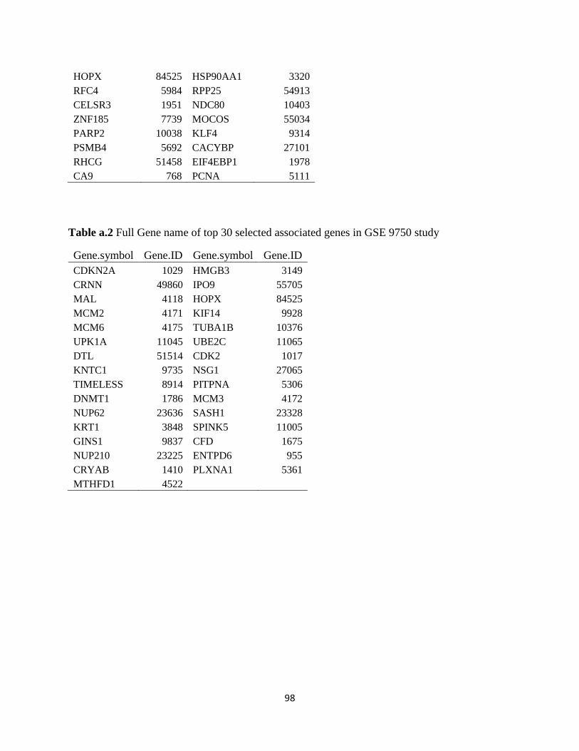
98

HOPX 84525 HSP90AA1 3320

RFC4 5984 RPP25 54913

CELSR3 1951 NDC80 10403

ZNF185 7739 MOCOS 55034

PARP2 10038 KLF4 9314

PSMB4 5692 CACYBP 27101

RHCG 51458 EIF4EBP1 1978

CA9 768 PCNA 5111

Table a.2 Full Gene name of top 30 selected associated genes in GSE 9750 study

Gene.symbol Gene.ID Gene.symbol Gene.ID

CDKN2A 1029 HMGB3 3149

CRNN 49860 IPO9 55705

MAL 4118 HOPX 84525

MCM2 4171 KIF14 9928

MCM6 4175 TUBA1B 10376

UPK1A 11045 UBE2C 11065

DTL 51514 CDK2 1017

KNTC1 9735 NSG1 27065

TIMELESS 8914 PITPNA 5306

DNMT1 1786 MCM3 4172

NUP62 23636 SASH1 23328

KRT1 3848 SPINK5 11005

GINS1 9837 CFD 1675

NUP210 23225 ENTPD6 955

CRYAB 1410 PLXNA1 5361

MTHFD1 4522

99

Table a.3 Full Gene name of 19 selected associated genes in TCGA cervical cancer study

Gene.Symbol

BEND7.222389

C17orf28.283987

DDAH1.23576

DEPDC6.64798

DNALI1.7802

ENPP4.22875

EPCAM.4072

FAM47E.100129583

FREM2.341640

GPR87.53836

HNF4G.3174

KCTD14.65987

P4HTM.54681

PLCH1.23007

PPP1R9A.55607

RGL3.57139

SLC6A20.54716

SORBS2.8470

TIGD4.201798

Feature selection and classification for high-dimensional ...

Documents

Transcript of Feature selection and classification for high-dimensional ...